Joint Bistatic Positioning and Monostatic Sensing: Optimized Beamforming and Performance Tradeoff

Abstract

We investigate joint bistatic positioning (BP) and monostatic sensing (MS) within a multi-input multi-output orthogonal frequency-division system. Based on the derived Cramér-Rao Bounds (CRBs), we propose novel beamforming optimization strategies that enable flexible performance trade-offs between BP and MS. Two distinct objectives are considered in this multi-objective optimization problem, namely, enabling user equipment to estimate its own position while accounting for unknown clock bias and orientation, and allowing the base station to locate passive targets. We first analyze digital schemes, proposing both weighted-sum CRB and weighted-sum mismatch (of beamformers and covariance matrices) minimization approaches. These are examined under full-dimension beamforming (FDB) and low-complexity codebook-based power allocation (CPA). To adapt to low-cost hardwares, we develop unit-amplitude analog FDB and CPA schemes based on the weighted-sum mismatch of the covariance matrices paradigm, solved using distinct methods. Numerical results confirm the effectiveness of our designs, highlighting the superiority of minimizing the weighted-sum mismatch of covariance matrices, and the advantages of mutual information fusion between BP and MS.

I Introduction

isac represents one of the most transformative shifts in 6G networks, merging sensing and communication capabilities and exploiting the mutualistic mechanism to enable a wide range of novel applications[1, 2, 3, 4, 5, 6]. Sensing, in this context, refers to a network’s ability to detect, locate, and interpret information about objects or users within its environment, facilitating applications that leverage both communication and sensing information, such as autonomous navigation, environmental monitoring, and location-based/aware services[6, 7, 8, 9, 10]. In general, sensing can be classified into sensing connected devices (e.g., via time-of-arrival-based positioning) and passive objects (e.g., via mono-/bi-/multi-static sensing) [8, 5, 6]. These two paradigms differ in their hardware and algorithmic requirements but can complement each other to enhance the network’s overall sensing capability[11, 6].

Positioning of a connected device is widely adopted in current systems with the support of Global Navigation Satellite Systems and, more recently, cellular networks to support in urban and suburban areas where satellite visibility is often limited[12, 7]. Specifically, the specification of positioning in 4G was introduced with the 3rd Generation Partnership Project (3GPP) Release 9, aiming to meet the regulatory requirement of 50-meter accuracy a user equipment (UE). The potential of positioning in 5G has been evaluated since 3GPP Release 15, and more ambitious efforts to achieve ultra-high accuracy, in conjunction with integrated sensing and communication (ISAC) for 6G, have been explored in Releases 18, 19, and beyond [13, 10, 6]. The evolution of communication systems has attracted considerable research attention in recent years. However, positioning connected devices requires the target to be part of the network that can transmit and receive pilot signals, and the sensing of passive objects is largely ignored.

ms originates from radar technology, which has been widely used for military and civilian air surveillance[14]. In modern networks, especially with the higher frequencies anticipated in 6G, monostatic sensing (MS) allows base stations to act as multi-functional nodes, combining communication with radar-like sensing capabilities[6, 15]. The expanded array apertures and bandwidths available in high-frequency bands, such as millimeter wave and sub-terahertz, significantly enhance the spatial and temporal resolution of estimation and hence the environment sensing performance [7]. Leveraging these capabilities, ISAC has demonstrated substantial potential in enabling perceptive mobile networks[16, 17] and facilitating predictive beamforming in high-mobility scenarios[18, 19]. Although MS in communication systems has yet to be standardized, the International Telecommunication Union’s Radio Communication Division technical report identifies ISAC as a primary usage scenario, underscoring the indispensable role of MS in its implementation [20].

In contrast, bistatic and multistatic sensing does not require full-duplex capability at the anchor, allowing for spatial diversity and extended coverage, which benefits various network applications[21]. All these mentioned techniques can sense passive targets, complementing positioning functions. Considering the dynamic characteristics of the network, especially when the mobile users are part of the sensing tasks of passive objects, simultaneously positioning active devices and mapping environmental targets within a bistatic setup [22, 23, 24, 11, 25], which is termed as bistatic positioning (BP) in this work. However, challenges such as the need for precise synchronization and orientation management between the transmitter and receiver must be overcome[10].

Besides sensing modes and scenarios, beamforming optimization has been a key area of research in ISAC, enhancing both sensing and communication performance and enabling effective tradeoffs between them. To balance these objectives, a common design criterion is to approximate an ideal multi-input-multi-output (MIMO) radar beampattern while meeting communication performance requirements through beamforming optimization [26, 27, 28, 29]. Extending this approach, recent studies [30, 31] have employed the Cramér-Rao bound (CRB) to quantify sensing performance, allowing a more precise characterization of the sensing-communication tradeoff in ISAC systems. Furthermore, beamforming design in ISAC has progressed from transmitter-only configurations to integrated transceiver designs [32, 33, 34].

Most of the aforementioned works focus on optimized beamforming for the efficient integration of radar-like MS and communications, while overlooking beamforming design for BP, which plays an increasingly important role in the generational upgrades of cellular networks [6]. The authors of [35] examined the BP setup with clock bias, shedding light on the properties of optimal beamforming. In [36], the beamforming design for BP was extended to the reconfigurable intelligent surface (RIS)-aided scenarios, enabling efficient joint BS-RIS beamforming for improved BP performance. As ISAC advances toward 6G, both BP and MS are expected to coexist, and it is crucial to understand the tradeoff between these two paradigms to achieve complementary strengths. However, it should be noted that BP and MS are typically studied independently, with limited attention given to their coexistence. The authors of [11] initiated research on integrating BP and MS from a simultaneous localization and mapping perspective. However, no existing works have designed beamformers to balance the tradeoff between these two paradigms.

In this paper, we explore the joint tasks of BP and MS within a representative MIMO orthogonal frequency division multiplexing (OFDM) framework, proposing effective beamforming designs that enable a flexible performance tradeoff between BP and MS, as characterized by the CRB. Our key contributions are summarized as follows.

• To optimize BP and MS jointly and strike a tradeoff between BP and MS, we formulate a multi-objective optimization (MOO) problem for beamforming design.

  • Starting with digital beamforming schemes, a weighted-sum CRB approach is proposed and solved using the full-dimensional beamforming (FDB) method to ensure a weak Pareto frontier. This reveals the optimal beamforming structure, which in turn leads to a low-complexity codebook-based power allocation (CPA) method. Additionally, weighted-sum mismatch minimization approaches, commonly used in balance-pursuit problems, are introduced under two distinct paradigms: beamformer mismatch and covariance matrix mismatch. These approaches are solved using both the FDB and CPA methods.

  • As hardware-efficient alternatives, analog beamforming schemes are proposed based on the weighted-sum mismatch of covariance matrices. Using an alternating optimization (AO) framework, we propose an FDB method, where each alternation is solved through sequential quadratic programming (SQP). Subsequently, we introduce an analog CPA method based on analog codebook construction.

• Comprehensive numerical results are presented to validate the effectiveness of the proposed beamforming schemes and to reveal the fundamental tradeoff between BP and MS. Specifically, we highlight the advantage of minimizing the weighted-sum mismatch of covariance matrices for beamforming, as it approaches the performance frontier achieved by the weighted-sum CRB approach. This finding supports the adoption of this paradigm when designing analog schemes. Furthermore, the results showcase the significant benefits of fusing common information between BP and MS, underscoring the importance of leveraging the mutualistic mechanism between BP and MS in practical system design.

The remainder of the paper is organized as follows. Section II introduces the system model and formulates the problem. Sections III and IV present digital beamforming designs based on the weighted-sum CRB and weighted-sum mismatch approaches, respectively. In Section V, we propose analog beamforming methods based on the weighted-sum mismatch of covariance matrices. Section VI provides an analysis of convergence and complexity, followed by numerical results in Section VII. Finally, Section VIII concludes the paper.

The primary notations used throughout this paper are defined as follows. Regular lowercase letters denote scalars, bold lowercase letters denote vectors, and bold uppercase letters represent matrices. The 2-norm of a vector $\mathbf{a}$ is denoted by $\left\|\mathbf{a}\right\|$, while the Frobenius norm of a matrix $\mathbf{A}$ is denoted by $\left\|\mathbf{A}\right\|_{\text{F}}$. Superscripts $\mathsf{T}$ and $\mathsf{H}$ indicate the transpose and Hermitian transpose of a vector or matrix, respectively. Additionally, $\text{tr}(\mathbf{A})$ and $\text{rank}(\mathbf{A})$ denote the trace and rank of matrix $\mathbf{A}$, and $\mathbf{A}\succeq\mathbf{0}$ indicates that matrix $\mathbf{A}$ is Hermitian and positive semi-definite. The real and imaginary parts of a scalar $a$ are represented by $\Re\left\{a\right\}$ and $\Im\left\{a\right\}$, respectively. $\text{diag}(\mathbf{a})$ represents a diagonal matrix with elements of $\mathbf{a}$ on its diagonal. Lastly, $\mathcal{CN}(\bm{\mu},\mathbf{C})$ denotes a circularly symmetric complex Gaussian (CSCG) distribution with mean $\bm{\mu}$ and covariance matrix $\mathbf{C}$.

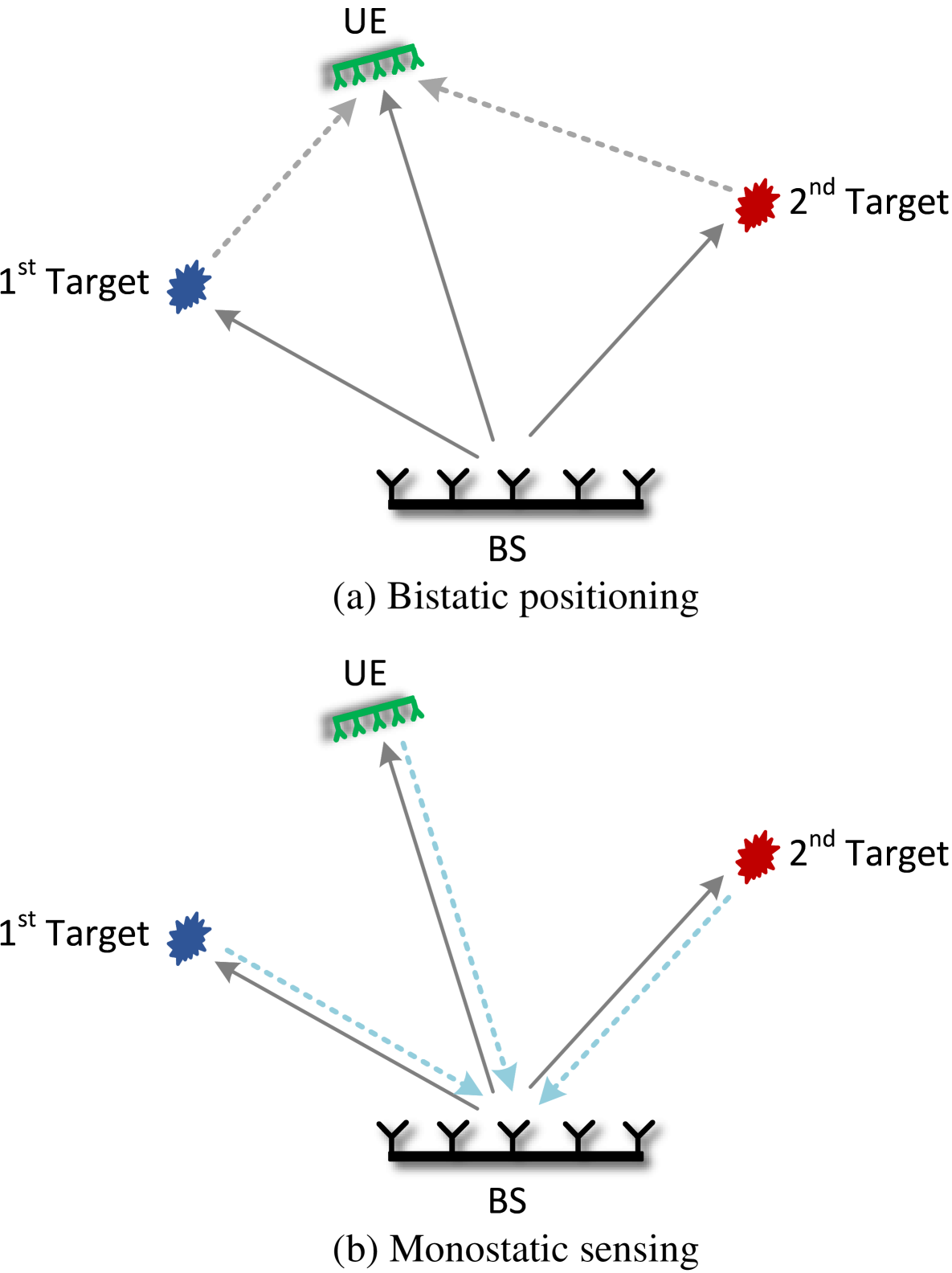
Figure 1: Illustration of joint (a) BP and (b) MS, where the BS transmits pilot signals, functioning as a monostatic radar to sense passive targets and the UE. Meanwhile, the UE uses the received pilot signals to position itself.

II System Model And Problem Formulation

II-A Signal Model

As illustrated in Fig. 1, we consider a MIMO OFDM-based joint BP and MS system with $M$ subcarriers, where a BS equipped with $N_{\text{B}}$ transmit antennas transmits positioning pilot signals across $L$ slots to a UE equipped with $N_{\text{U}}$ antennas, who uses the received signals to positioning itself, referred to as BP. Meanwhile, the BS acts as a monostatic radar with $N_{\text{B}}$ colocated receive antennas, sensing the environments by receiving echoes from passive targets and the UE, then estimating their positions, referred to as MS. In the system, a passive target in MS creates one multipath in BP.

Let $P$ denote the number of OFDM pilot symbols in each slot. The transmit signal associated with the $p$-th symbol in the $l$-th slot over the $m$-th subcarrier is given by

$$\bm{x}_{l,p,m}=\bm{f}_{l}s_{p,m},$$ (1)

where $\bm{f}_{l}\in\mathbb{C}^{N_{\text{B}}}$ is the beamformer for the $l$-th slot, and $s_{p,m}$ is the unit-modulus pilot symbol over the $m$-th subcarrier of the $p$-th symbol.

II-A1 Receive Signal at BP

The signal received at the UE is

$$\overline{\bm{y}}_{l,p,m}=\bm{W}^{\mathsf{H}}\overline{\bm{H}}_{m}\bm{x}_{l,p,m}+\overline{\bm{z}}_{l,p,m},$$ (2)

where $\bm{W}\in\mathbb{C}^{N_{\text{U}}\times N_{\text{U},\text{RF}}}$ is the analog combining matrix at the UE, with $N_{\text{U},\text{RF}}$ being the number of RF chains, $\overline{\bm{H}}_{m}\in\mathbb{C}^{N_{\text{U}}\times N_{\text{B}}}$ is the channel between the BS and the UE over the $m$-th subcarrier, given by

$$\overline{\bm{H}}_{m}=\sum_{k=0}^{K}\overline{\beta}_{k}e^{-\jmath 2\pi m\Delta f\overline{\tau}_{k}}\bm{a}_{\text{U}}\left(\psi_{k}\right)\bm{a}_{\text{B}}^{\mathsf{H}}\left(\theta_{k}\right),$$ (3)

and $\overline{\bm{z}}_{l,p,m}\sim\mathcal{CN}(\bm{0},\sigma^{2}\bm{I}_{N_{\text{U}}})$ is the additive white Gaussian noise (AWGN) at the UE receiver. Here, $\sigma^{2}=FN_{0}\Delta f$ is the noise power where $F$, $N_{0}$, and $\Delta f$ denote the noise figure, single-side power spectral density (PSD), and subcarrier spacing, respectively.

In (3), $K$ denotes the number of targets, and $\overline{\beta}_{k}$, $\overline{\tau}_{k}$, $\psi_{k}$, and $\theta_{k}$ are the complex channel gain, delay, angle-of-arrival (AOA), and angle-of-departure (AOD), respectively, associated with the $k$-th path. For notational convenience, the line-of-sight (LOS) path of the channel is indexed by $k=0$. Specifically, $\psi_{0}$ and $\theta_{0}$ denote the AOA and AOD with respect to the BS and the UE, respectively. Finally, $\bm{a}_{\text{B}}\left(\cdot\right)\in\mathbb{C}^{N_{\text{B}}}$ and $\bm{a}_{\text{U}}\left(\cdot\right)\in\mathbb{C}^{N_{\text{U}}}$ are the steering vectors at the BS (transmitter side) and the UE, respectively.

II-A2 Receive Signal at MS

Similarly, the signal received at the (colocated) BS receiver is

$$\underline{\bm{y}}_{l,p,m}=\underline{\bm{H}}_{m}\bm{x}_{l,p,m}+\underline{\bm{z}}_{l,p,m},$$ (4)

where $\underline{\bm{H}}_{m}\in\mathbb{C}^{N_{\text{B}}\times N_{\text{B}}}$ is the round-trip channel between the BS and the passive targets (including the UE) over the $m$-th subcarrier, given by

$$\underline{\bm{H}}_{m}=\sum_{k=0}^{K}\underline{\beta}_{k}e^{-\jmath 2\pi m\Delta f\underline{\tau}_{k}}\bm{a}_{\text{B}}\left(\theta_{k}\right)\bm{a}_{\text{B}}^{\mathsf{H}}\left(\theta_{k}\right),$$ (5)

and $\underline{\bm{z}}_{l,p,m}\sim\mathcal{CN}(\bm{0},\sigma^{2}\bm{I}_{N_{\text{B}}})$ is the AWGN at the BS receiver. Here, $\underline{\beta}_{k}$ and $\underline{\tau}_{k}$ represent the complex channel gain and delay, respectively, associated with the $k$-th object. Here, UE is also an target, indexed by $k=0$, in the MS scenario.

II-B CRB-Based Performance Metric

For both BP and MS, we consider a two-stage positioning process, where the channel-domain parameters are estimated in the first stage, followed by the inference of position-domain parameters in the second stage.

II-B1 Performance Metric of BP

In BP, the channel-domain parameters are collected by $\overline{\bm{\xi}}=[\bm{\theta}^{\mathsf{T}},\bm{\psi}^{\mathsf{T}},\overline{\bm{\tau}}^{\mathsf{T}},\bm{\overline{\beta}}_{\text{R}}^{\mathsf{T}},\bm{\overline{\beta}}_{\text{I}}^{\mathsf{T}}]^{\mathsf{T}}\in\mathbb{R}^{(5K+5)}$, where $\bm{\theta}=[{\theta}_{0},\ldots,{\theta}_{K}]^{\mathsf{T}}\in\mathbb{R}^{(K+1)}$ is the collection of AODs, $\bm{\psi}=[{\psi}_{0},\ldots,{\psi}_{K}]^{\mathsf{T}}\in\mathbb{R}^{(K+1)}$ is the collection of AOAs, $\overline{\bm{\tau}}=[{\overline{\tau}}_{0},\ldots,{\overline{\tau}}_{K}]^{\mathsf{T}}\in\mathbb{R}^{(K+1)}$ represents the delays, and $\bm{\overline{\beta}}_{\text{R}}=[\Re\{{\overline{\beta}}_{0}\},\ldots,\Re\{{\overline{\beta}}_{K}\}]^{\mathsf{T}}\in\mathbb{R}^{(K+1)}$ and $\bm{\overline{\beta}}_{\text{I}}=[\Im\{{\overline{\beta}}_{0}\},\ldots,\Im\{{\overline{\beta}}_{K}\}]^{\mathsf{T}}\in\mathbb{R}^{(K+1)}$ are the collections of the real and imaginary parts of the complex channel gains, respectively. Using the Slepian-Bangs formula[35], the element at the $i$-th row and $j$-th column of the channel-domain Fisher information matrix (FIM) $\bm{I}_{\text{Chan}}(\overline{\bm{\xi}})$ is derived as

$$\begin{aligned} \left[\bm{I}_{\text{Chan}}\left(\overline{\bm{\xi}}\right)\right]_{i,j}&=\frac{2}{\sigma^{2}}\sum_{l=1}^{L}\sum_{p=1}^{P}\sum_{m=1}^{M}\Re\left\{\frac{\partial\overline{\bm{\mu}}_{l,p,m}^{\mathsf{H}}}{\partial\left[\overline{\bm{\xi}}\right]_{i}}\frac{\partial\overline{\bm{\mu}}_{l,p,m}}{\partial\left[\overline{\bm{\xi}}\right]_{j}}\right\}\\ &=\frac{2N}{\sigma^{2}}\sum_{m=1}^{M}\Re\left\{\text{tr}\left(\frac{\partial\overline{\bm{H}}_{m}}{\partial\left[\overline{\bm{\xi}}\right]_{j}}\bm{F}\bm{F}^{\mathsf{H}}\frac{\partial\overline{\bm{H}}_{m}^{\mathsf{H}}}{\partial\left[\overline{\bm{\xi}}\right]_{i}}\right)\right\},\end{aligned}$$ (6)

where $\overline{\bm{\mu}}_{l,p,m}=\overline{\bm{H}}_{m}\bm{x}_{l,p,m}$ denotes the noise-free observation from (2) and $\bm{F}=[\bm{f}_{1},\ldots,\bm{f}_{L}]\in\mathbb{C}^{N_{\text{B}}\times L}$ collects $L$ beamformers.

The position-domain parameters are collected in $\overline{\bm{\eta}}=[\bm{p}_{\text{U}}^{\mathsf{T}},\Delta\phi,\bm{p}_{1}^{\mathsf{T}},\ldots,\bm{p}_{K}^{\mathsf{T}},\Delta t,\bm{\overline{\beta}}_{\text{R}}^{\mathsf{T}},\bm{\overline{\beta}}_{\text{I}}^{\mathsf{T}}]^{\mathsf{T}}\in\mathbb{R}^{(4K+6)}$, where $\bm{p}_{\text{U}}\in\mathbb{R}^{2}$ represents the position of the UE, and $\bm{p}_{k}\in\mathbb{R}^{2}$ represents the position of the $k$-th object. The variable $\Delta\phi$ denotes the relative orientation of the BS (in the UE’s local coordinate system), while $\Delta t$ characterizes the clock bias that reflects the asynchronism between the BS and UE in the bistatic setting. Note that the nuisance parameters $\bm{\overline{\beta}}_{\text{R}}$ and $\bm{\overline{\beta}}_{\text{I}}$ from the channel-domain parameter $\overline{\bm{\xi}}$ remain part of the position-domain parameter $\overline{\bm{\eta}}$, as they do not contribute useful information for position estimation. Using the channel-domain FIM, the position-domain FIM $\bm{I}_{\text{Pos}}(\overline{\bm{\eta}})$ is computed as follows

$$\bm{I}_{\text{Pos}}\left(\overline{\bm{\eta}}\right)=\overline{\bm{J}}^{\mathsf{T}}\bm{I}_{\text{Chan}}\left(\overline{\bm{\xi}}\right)\overline{\bm{J}},$$ (7)

where $\overline{\bm{J}}\in\mathbb{R}^{(5K+5)\times(4K+6)}$ is the Jacobian matrix, with the element in the $i$-th row and $j$-th column given by $[\overline{\bm{J}}]_{i,j}=\partial[\overline{\bm{\xi}}]_{i}/\partial[\overline{\bm{\eta}}]_{j}$. The CRB is used to quantify the BP accuracy concerning $\bm{p}_{\text{U}}$, providing a lower bound on the sum of the covariances for estimating $\bm{p}_{\text{U}}$, and is expressed as

$$\overline{\text{CRB}}\left(\bm{p}_{\text{U}}\right)=\text{tr}\left(\left[\bm{I}_{\text{Pos}}\left(\overline{\bm{\eta}}\right)^{-1}\right]_{1:2,1:2}\right).$$ (8)

II-B2 Performance Metric of MS

Following similar steps, the position-domain FIM for MS is given by

$$\bm{I}_{\text{Pos}}\left(\underline{\bm{\eta}}\right)=\underline{\bm{J}}^{\mathsf{T}}\bm{I}_{\text{Chan}}\left(\underline{\bm{\xi}}\right)\underline{\bm{J}},$$ (9)

where $\underline{\bm{\xi}}=[\bm{\theta}^{\mathsf{T}},\bm{\underline{\tau}}^{\mathsf{T}},\bm{\underline{\beta}}_{\text{R}}^{\mathsf{T}},\bm{\underline{\beta}}_{\text{I}}^{\mathsf{T}}]^{\mathsf{T}}\in\mathbb{R}^{(4K+4)}$ and $\underline{\bm{\eta}}=[\bm{p}_{\text{U}}^{\mathsf{T}},\bm{p}_{1}^{\mathsf{T}},\ldots,\bm{p}_{K}^{\mathsf{T}},\bm{\underline{\beta}}_{\text{R}}^{\mathsf{T}},\bm{\underline{\beta}}_{\text{I}}^{\mathsf{T}}]^{\mathsf{T}}\in\mathbb{R}^{(4K+4)}$ are the channel-domain and position-domain parameters, respectively. Here, $\bm{\underline{\tau}}=[{\underline{\tau}}_{0},\ldots,{\underline{\tau}}_{K}]^{\mathsf{T}}\in\mathbb{R}^{(K+1)}$ represents the delay measurements, while $\bm{\underline{\beta}}_{\text{R}}=[\Re\{{\underline{\beta}}_{0}\},\ldots,\Re\{{\underline{\beta}}_{K}\}]^{\mathsf{T}}\in\mathbb{R}^{(K+1)}$ and $\bm{\underline{\beta}}_{\text{I}}=[\Im\{{\underline{\beta}}_{0}\},\ldots,\Im\{{\underline{\beta}}_{K}\}]^{\mathsf{T}}\in\mathbb{R}^{(K+1)}$ represent the real and imaginary parts of the complex channel gains, respectively. The CRB for MS, concerning the passive targets (as well as the UE), provides a lower bound on the sum covariance for estimating $\bm{p}=[\bm{p}_{\text{U}}^{\mathsf{T}},\bm{p}_{1}^{\mathsf{T}},\ldots,\bm{p}_{K}^{\mathsf{T}}]^{\mathsf{T}}\in\mathbb{R}^{(2K+2)}$ at the BS, and is given by

$$\underline{\text{CRB}}\left(\bm{p}\right)=\text{tr}\left(\left[\bm{I}_{\text{Pos}}\left(\underline{\bm{\eta}}\right)^{-1}\right]_{1:2K+2,1:2K+2}\right).$$ (10)

II-C Problem Formulation

We observe that both $\overline{\text{CRB}}(\bm{p}_{\text{U}})$ and $\underline{\text{CRB}}(\bm{p})$ are functions of $\bm{F}$, which can be optimized by designing the beamformers $\bm{F}$[35, 36]. However, due to the different objectives, a performance tradeoff between BP and MS emerges. Specifically, this bistatic-monostatic performance tradeoff is characterized by a MOO problem[38], expressed as

$$\mathop{\min}\limits_{\bm{F}}\;\;\; \left[\overline{\text{CRB}}\left(\bm{p}_{\text{U}}\right),\underline{\text{CRB}}\left(\bm{p}\right)\right]$$ (11a)

$${\rm{s.t.}}\;\;\; \text{tr}\left(\bm{F}\bm{F}^{\mathsf{H}}\right)\leq P_{\text{B}}/M,$$ (11b)

where $P_{\text{B}}$ is the power budget. Without loss of generality, the right-hand side of (11b) is set as $P_{\text{B}}/M$ such that the total transmit power over $M$ subcarriers is $P$. Note that the optimal solution to (11) represents the Pareto frontier of $[\overline{\text{CRB}}(\bm{p}_{\text{U}}),\underline{\text{CRB}}(\bm{p})]$, which is challenging to find due to the MOO nature. Additionally, neither $\overline{\text{CRB}}(\bm{p}_{\text{U}})$ nor $\underline{\text{CRB}}(\bm{p})$ is convex with respect to $\bm{F}$, further complicating the problem.

Remark 1.

We would like to emphasize that in the previous formulation, the BP and MS components of the system are treated independently, with no exchange of information between them. However, it is important to recognize that, although positioning targets is not the primary goal of BP, it remains a fundamental requirement, as does positioning the UE. Therefore, despite operating in different configurations, both BP and MS share the common objective of jointly positioning the targets and the UE. To understand the performance limits of joint BP and MS, we can leverage a mutualistic approach by combining the information from both components (assuming the existence of a feedback channel between the BS and UE), thus forming a bounding framework. Specifically, the fused position-domain parameters are aggregated as $\underline{\overline{\bm{\eta}}}=[\bm{p}_{1}^{\mathsf{T}},\ldots,\bm{p}_{K}^{\mathsf{T}},\bm{p}_{\text{U}}^{\mathsf{T}},\Delta\phi,\Delta t,\bm{\overline{\beta}}_{\text{R}}^{\mathsf{T}},\bm{\overline{\beta}}_{\text{I}}^{\mathsf{T}},\bm{\underline{\beta}}_{\text{R}}^{\mathsf{T}},\bm{\underline{\beta}}_{\text{I}}^{\mathsf{T}}]^{\mathsf{T}}\in\mathbb{R}^{(6K+6)}$. The elements of the fused position-domain FIM, denoted as $\bm{I}_{\text{Pos}}(\underline{\overline{\bm{\eta}}})$, are obtained by either replicating the exclusive terms from the position-domain FIM of BP or MS, or summing the relevant terms from both. The fused CRB for BP, denoted as $\underline{\overline{\text{CRB}}}(\bm{p}_{\text{U}})$, and the fused CRB for MS, denoted as $\underline{\overline{\text{CRB}}}(\bm{p})$, can be derived from $\bm{I}_{\text{Pos}}(\underline{\overline{\bm{\eta}}})$ by inverting it and extracting the appropriate trace terms. Additionally, although the beamforming methods we develop in the subsequent sections are based on the non-fused scenario, they can be extended to the fused case by solving a similar MOO problem as in (11) using the fused CRBs.

III Weighted-Sum CRB Optimization

To address (11) and explore the performance tradeoff, we begin by applying the weighted-sum method, a well-established technique for obtaining the weak Pareto frontier of MOO problems[38]. Using this method, we formulate and solve an FDB optimization problem aimed at optimizing the beamformers $\bm{F}$. Additionally, we reveal the characteristics of the optimal solution, which motivates the development of a CPA approach that balances BP and MS with reduced complexity, serving as a complementary solution to the FDB method.

III-A Full-Dimensional Beamforming

With FDB, we retain the beamformers $\bm{F}$ as the optimization variable. Under the weighted-sum approach, the problem in (11) is then reformulated as

$$\mathop{\min}\limits_{\bm{F}}\;\;\; \alpha\overline{\text{CRB}}\left(\bm{p}_{\text{U}}\right)+\left(1-\alpha\right)\underline{\text{CRB}}\left(\bm{p}\right)$$ (12a)

$${\rm{s.t.}}\;\;\; \text{tr}\left(\bm{F}\bm{F}^{\mathsf{H}}\right)\leq P_{\text{B}}/M,$$ (12b)

where $\alpha\in[0,1]$ is a constant that adjusts the priority between BP and MS, determined by the specific application scenario and quality of service (QoS) requirements.

Problem (12) remains challenging to solve due to its non-convexity. By defining $\bm{V}=\bm{F}\bm{F}^{\mathsf{H}}$, we lift (12) into a relaxed form (by omitting the constraint $\text{rank}(\bm{V})=L$) as

$$\mathop{\min}\limits_{\bm{V}}\;\;\; \alpha\overline{\text{CRB}}\left(\bm{p}_{\text{U}}\right)+\left(1-\alpha\right)\underline{\text{CRB}}\left(\bm{p}\right)$$ (13a)

$${\rm{s.t.}}\;\;\; \text{tr}\left(\bm{V}\right)\leq P_{\text{B}}/M,\quad\bm{V}\succeq\mathbf{0}.$$ (13b)

Next, note that the matrices on the right-hand sides of (8) and (10) can be reformulated as[23]

$$\left[\bm{I}_{\text{Pos}}\left(\overline{\bm{\eta}}\right)^{-1}\right]_{1:2,1:2}=\left[\overline{\bm{Y}}-\overline{\bm{G}}\overline{\bm{Z}}^{-1}\overline{\bm{G}}^{\mathsf{T}}\right]^{-1},$$ (14a)

$$\left[\bm{I}_{\text{Pos}}\left(\underline{\bm{\eta}}\right)^{-1}\right]_{1:2K+2,1:2K+2}=\left[\underline{\bm{Y}}-\underline{\bm{G}}\underline{\bm{Z}}^{-1}\underline{\bm{G}}^{\mathsf{T}}\right]^{-1},$$ (14b)

where $\overline{\bm{Y}}=[\bm{I}_{\text{Pos}}(\overline{\bm{\eta}})]_{1:2,1:2}$, $\overline{\bm{G}}=[\bm{I}_{\text{Pos}}(\overline{\bm{\eta}})]_{1:2,3:4K+6}$, $\overline{\bm{Z}}=[\bm{I}_{\text{Pos}}(\overline{\bm{\eta}})]_{3:4K+6,3:4K+6}$, $\underline{\bm{Y}}=[\bm{I}_{\text{Pos}}(\underline{\bm{\eta}})]_{1:2K+2,1:2K+2}$, $\underline{\bm{G}}=[\bm{I}_{\text{Pos}}(\underline{\bm{\eta}})]_{1:2K+2,2K+3:4K+4}$, and $\underline{\bm{Z}}=[\bm{I}_{\text{Pos}}(\underline{\bm{\eta}})]_{2K+3:4K+4,2K+3:4K+4}$. By introducing auxiliary variables $\overline{\bm{U}}\in\mathbb{R}^{2\times 2}$ and $\underline{\bm{U}}\in\mathbb{R}^{(2K+2)\times(2K+2)}$, (13) can be reformulated into an equivalent form as

$$\mathop{\min}\limits_{\bm{V},\overline{\bm{U}},\underline{\bm{U}}}\;\;\; \alpha\text{tr}\left(\overline{\bm{U}}^{-1}\right)+\left(1-\alpha\right)\text{tr}\left(\underline{\bm{U}}^{-1}\right)$$ (15a)

$${\rm{s.t.}}\;\;\; \begin{bmatrix}\overline{\bm{Y}}-\overline{\bm{U}}&\overline{\bm{G}}\\ \overline{\bm{G}}^{\mathsf{T}}&\overline{\bm{Z}}\end{bmatrix}\succeq\mathbf{0},\quad\begin{bmatrix}\underline{\bm{Y}}-\underline{\bm{U}}&\underline{\bm{G}}\\ \underline{\bm{G}}^{\mathsf{T}}&\underline{\bm{Z}}\end{bmatrix}\succeq\mathbf{0},$$ (15b)

$$\overline{\bm{U}}\succeq\mathbf{0},\quad\underline{\bm{U}}\succeq\mathbf{0},$$ (15c)

$$\text{tr}\left(\bm{V}\right)\leq P_{\text{B}}/M,\quad\bm{V}\succeq\mathbf{0}.$$ (15d)

The above problem is a convex semi-definite programming (SDP) problem that can be efficiently solved using off-the-shelf optimization tools such as CVX. Once solved, the beamformers $\bm{F}$ can be recovered from $\bm{V}$ via matrix decomposition or a randomization procedure[39].

Remark 2.

Following similar reasoning to that in Appendix C of [40], we point out that the optimal covariance matrix that minimizes the CRB can be expressed as $\bm{V}=\bm{U}\bm{\Lambda}\bm{U}^{\mathsf{H}}$, where $\bm{\Lambda}\in\mathbb{C}^{\left(2K+2\right)\times\left(2K+2\right)}$ is a positive semi-definite matrix and $\bm{U}=[\bm{a}_{\text{B}}\left(\theta_{0}\right),\ldots,\bm{a}_{\text{B}}\left(\theta_{K}\right),\dot{\bm{a}}_{\text{B}}\left(\theta_{0}\right),\ldots,\dot{\bm{a}}_{\text{B}}\left(\theta_{K}\right)]\in\mathbb{C}^{N_{\text{B}}\times\left(2K+2\right)}$, with $\dot{\bm{a}}_{\text{B}}\left(\theta_{0}\right)=\partial\bm{a}_{\text{B}}\left(\theta_{k}\right)/\partial\theta_{k}$. It is important to note that although this property was derived under single CRB minimization (rather than weighted-sum minimization as in (13)), the derivation in [40] can be straightforwardly extended to our case since the BP and MS components share the same $\bm{U}$. Therefore, it is omitted here for brevity. The revealed optimal structure of the solution can be applied to solve the SDP problem in (15), i.e., by optimizing $\bm{\Lambda}$ instead of $\bm{V}$, which significantly reduces the complexity. This is because the dimension of $\bm{\Lambda}$, determined by the number of targets, is typically much smaller than that of $\bm{V}$, which is determined by the number of transmit antennas.

III-B Codebook-based Power Allocation

By constraining $\bm{\Lambda}$ to be diagonal, the FDB method is reduced to a lower-dimensional, lower-complexity power allocation scheme over the predetermined codebook matrix $\bm{U}$. Let $\bm{\rho}=[\rho_{1},\ldots,\rho_{2K+2}]$ be the power allocation vector. We propose a CPA method by substituting the variable $\bm{V}$ in (13) with $\bm{U}\text{diag}\left(\bm{\rho}\right)\bm{U}^{\mathsf{H}}$. The resulting power allocation problem is then given by

$$\mathop{\min}\limits_{\bm{\rho}}\;\;\; \alpha\overline{\text{CRB}}\left(\bm{p}_{\text{U}}\right)+\left(1-\alpha\right)\underline{\text{CRB}}\left(\bm{p}\right)$$ (16a)

$${\rm{s.t.}}\;\;\; \text{tr}\left(\bm{U}\text{diag}\left(\bm{\rho}\right)\bm{U}^{\mathsf{H}}\right)\leq\frac{P}{M},\quad\bm{\rho}\geq\bm{0},$$ (16b)

where $\bm{\rho}\geq\bm{0}$ ensures all elements of $\bm{\rho}$ are non-negative. Using similar steps as in the previous subsection, (16) can be reformulated into a form that can be efficiently solved by standard tools, which is omitted to avoid redundancy.

IV Weighted-Sum Mismatch Approaches

Building on the weighted waveform mismatch minimization approach commonly employed in the ISAC literature to balance sensing and communication performance [27, 41], we propose alternative methods for both FDB and CPA to strike an effective tradeoff between BP and MS by minimizing the weighted-sum mismatch of two distinct metrics. Specifically, the optimal beamformers, $\overline{\bm{F}}$ for BP and $\underline{\bm{F}}$ for MS, are obtained by solving (15) and (16) with $\alpha=1$ and $\alpha=0$, respectively. The balanced beamformers are then derived from these extremes by applying different strategies: one approach minimizes the weighted-sum mismatch of the beamformers, while the other focuses on minimizing the weighted-sum mismatch of the covariance matrices.

IV-A Weighted-Sum Mismatch of Beamformers

IV-A1 FDB

Upon obtaining $\overline{\bm{F}}$ and $\underline{\bm{F}}$ by solving (15) with $\alpha=1$ and $\alpha=0$, respectively, we formulate the following optimization problem to minimize the weighted-sum mismatch of beamformers

$$\mathop{\min}\limits_{\bm{F}}\;\;\; \alpha\left\|\bm{F}-\overline{\bm{F}}\right\|_{\text{F}}^{2}+\left(1-\alpha\right)\left\|\bm{F}-\underline{\bm{F}}\right\|_{\text{F}}^{2}$$ (17a)

$${\rm{s.t.}}\;\;\; \text{tr}\left(\bm{F}\bm{F}^{\mathsf{H}}\right)=P_{\text{B}}/M,$$ (17b)

where (17b) represents the full power transmission constraint.

Inspired by Remark 2, we define $\bm{F}=\bm{U}\bm{\Omega}$, where $\bm{\Omega}=[\bm{\omega}_{1},\ldots,\bm{\omega}_{2K+2}]\in\mathbb{C}^{(2K+2)\times(2K+2)}$, ensuring that $\bm{F}\bm{F}^{\mathsf{H}}$ satisfies the properties of the optimal covariance matrix. This formulation not only steers the solution toward the desired structure but also decreases complexity by reducing the dimensionality of the variables. Then, (17) can be reformulated as

$$\mathop{\min}\limits_{\bm{\Omega}}\;\;\; \left\|\bm{A}\bm{U}\bm{\Omega}-\bm{B}\right\|_{\text{F}}^{2}$$ (18a)

$${\rm{s.t.}}\;\;\; \text{tr}\left(\bm{U}\bm{\Omega}\bm{\Omega}^{\mathsf{H}}\bm{U}^{\mathsf{H}}\right)=P_{\text{B}}/M,$$ (18b)

where $\bm{A}=[\sqrt{\alpha}\mathbf{I}_{N_{\text{B}}};\sqrt{1-\alpha}\mathbf{I}_{N_{\text{B}}}]$ and $\bm{B}=[\sqrt{\alpha}\overline{\bm{F}};\sqrt{1-\alpha}\underline{\bm{F}}]$.

The problem remains non-convex due to the equality constraint in (18b). Notably, we have $\bm{A}^{\mathsf{H}}\bm{A}=\mathbf{I}_{N_{\text{B}}}$. By introducing $\bm{X}=\bm{U}^{\mathsf{H}}\bm{A}^{\mathsf{H}}\bm{B}$ and $\tilde{\bm{\Omega}}_{l}=\tilde{\bm{\omega}}_{l}\tilde{\bm{\omega}}_{l}^{\mathsf{H}}$, where $\tilde{\bm{\omega}}_{l}=[1,\bm{\omega}_{l}^{\mathsf{T}}]^{\mathsf{T}}$, we can relax the constraint $\text{rank}(\tilde{\bm{\Omega}}_{l})=1$. This allows us to lift and reformulate (18) into

$$\mathop{\min}\limits_{\tilde{\bm{\Omega}}_{l}}\;\;\; \sum_{l=1}^{2K+2}\text{tr}\left(\begin{bmatrix}0&-\bm{X}_{:,l}^{\mathsf{H}}\\ -\bm{X}_{:,l}&\bm{U}^{\mathsf{H}}\bm{U}\end{bmatrix}\tilde{\bm{\Omega}}_{l}\right)$$ (19a)

$${\rm{s.t.}}\;\;\; \sum_{l=1}^{2K+2}\text{tr}\left(\begin{bmatrix}1&\bm{0}\\ \bm{0}&\bm{U}^{\mathsf{H}}\bm{U}\end{bmatrix}\tilde{\bm{\Omega}}_{l}\right)=P_{\text{B}}/M+L,$$ (19b)

$$\left[\tilde{\bm{\Omega}}_{l}\right]_{1,1}=1,\quad\tilde{\bm{\Omega}}_{l}\succeq\mathbf{0},\quad\forall l.$$ (19c)

The relaxed formulation in (19) results in a convex SDP problem. Despite the relaxation, this formulation fits into the class of trust-region subproblems, which are characterized by strong duality and guarantee rank-one solutions [42]. Consequently, the optimal $\tilde{\bm{\omega}}_{l}$, and hence the optimal $\bm{\omega}_{l}$ for (18), can be recovered from the obtained $\tilde{\bm{\Omega}}_{l}$, leading to the determination of $\bm{F}$.

IV-A2 CPA

Let $\bm{F}=\bm{U}\bm{\Upsilon}$, where $\bm{\Upsilon}=\text{diag}(\bm{\upsilon})$ and $\bm{\upsilon}=[\upsilon_{1},\ldots,\upsilon_{2K+2}]\in\mathbb{R}^{(2K+2)}$. The matrix $\bm{\Upsilon}\bm{\Upsilon}^{\mathsf{H}}$ is diagonal, representing the power allocation. The optimization problem for minimizing the weighted-sum mismatch of beamformers through power allocation is formulated as

$$\mathop{\min}\limits_{\bm{\upsilon}}\;\;\; \alpha\left\|\bm{U}\bm{\Upsilon}-\overline{\bm{F}}\right\|_{\text{F}}^{2}+\left(1-\alpha\right)\left\|\bm{U}\bm{\Upsilon}-\underline{\bm{F}}\right\|_{\text{F}}^{2}$$ (20a)

$${\rm{s.t.}}\;\;\; \text{tr}\left(\bm{U}\bm{\Upsilon}\bm{\Upsilon}^{\mathsf{H}}\bm{U}^{\mathsf{H}}\right)=P_{\text{B}}/M,$$ (20b)

where $\overline{\bm{F}}$ and $\underline{\bm{F}}$ are the beamformers obtained by solving (16) for $\alpha=1$ and $\alpha=0$, respectively.

Problem (20) is non-convex. However, after performing algebraic transformations, it can be relaxed as

$$\mathop{\min}\limits_{\tilde{\bm{\Upsilon}}_{l}}\;\;\; \sum_{l=1}^{2K+2}\text{tr}\left(\begin{bmatrix}0&-\Re\left\{\vartheta_{l}\right\}\\ -\Re\left\{\vartheta_{l}\right\}&\varpi_{l}\end{bmatrix}\tilde{\bm{\Upsilon}}_{l}\right)$$ (21a)

$${\rm{s.t.}}\;\;\; \sum_{l=1}^{2K+2}\text{tr}\left(\begin{bmatrix}1&0\\ 0&\bm{U}_{:,l}^{\mathsf{H}}\bm{U}_{:,l}\end{bmatrix}\tilde{\bm{\Upsilon}}_{l}\right)=P_{\text{B}}/M+L,$$ (21b)

$$\left[\tilde{\bm{\Upsilon}}_{l}\right]_{1,1}=1,\quad\tilde{\bm{\Upsilon}}_{l}\succeq\mathbf{0},\quad\forall l,$$ (21c)

where $\vartheta_{l}=\bm{\Gamma}_{:,l}^{\mathsf{H}}\bm{B}_{:,l}$ and $\varpi_{l}=\bm{\Gamma}_{:,l}^{\mathsf{H}}\bm{\Gamma}_{:,l}$, with $\bm{\Gamma}=\bm{A}\bm{U}$ and $\tilde{\bm{\Upsilon}}_{l}=\tilde{\bm{\upsilon}}_{l}\tilde{\bm{\upsilon}}_{l}^{\mathsf{H}}$, where $\tilde{\bm{\upsilon}}_{l}=[1,\upsilon_{l}]^{\mathsf{T}}$. Similarly, by invoking strong duality, the rank-one solutions are guaranteed[42]. The optimal $\tilde{\bm{\upsilon}}_{l}$, and consequently the optimal $\bm{\upsilon}$ for (20), can be derived from the obtained $\tilde{\bm{\Upsilon}}_{l}$, leading to obtaining $\bm{F}$.

IV-B Weighted-Sum Mismatch of Covariance Matrices

IV-B1 FDB

We observe that the position-domain FIM, and thus the CRBs in (8) and (10), are directly influenced by $\bm{F}\bm{F}^{\mathsf{H}}$. This term can be interpreted as the covariance matrix of the transmit signal (up to scaling), capturing the combined effect of different beamformers. Motivated by this insight, we propose minimizing the weighted sum mismatch of these covariance matrices. From the resulting covariance matrix, the beamformers can then be derived. Specifically, using the optimal form of the covariance matrix, represented as $\bm{V}=\bm{U}\bm{\Lambda}\bm{U}^{\mathsf{H}}$, we formulate the optimization problem as

$$\mathop{\min}\limits_{\bm{\Lambda}}\;\;\; \alpha\left\|\bm{U}\bm{\Lambda}\bm{U}^{\mathsf{H}}-\overline{\bm{V}}\right\|_{\text{F}}^{2}+\left(1-\alpha\right)\left\|\bm{U}\bm{\Lambda}\bm{U}^{\mathsf{H}}-\underline{\bm{V}}\right\|_{\text{F}}^{2}$$ (22a)

$${\rm{s.t.}}\;\;\; \text{tr}\left(\bm{U}\bm{\Lambda}\bm{U}^{\mathsf{H}}\right)=P_{\text{B}}/M,$$ (22b)

$$\bm{\Lambda}\succeq\bm{0},$$ (22c)

where $\overline{\bm{V}}=\overline{\bm{F}}\overline{\bm{F}}^{\mathsf{H}}$ and $\underline{\bm{V}}=\underline{\bm{F}}\underline{\bm{F}}^{\mathsf{H}}$.

The problem in (22) is a SDP, which can be efficiently solved using tools like CVX. Once the solution is obtained, the beamformers $\bm{F}$ can be extracted through matrix decomposition techniques.

IV-B2 CPA

For the weighted-sum mismatch of covariance matrices approach under the CPA scheme, we replace $\bm{\Lambda}$ in (22) with $\bm{U}\text{diag}\left(\bm{\rho}\right)\bm{U}^{\mathsf{H}}$ and modify (22c) to $\bm{\rho}\geq\bm{0}$. The resulting formulation is a convex quadratically constrained quadratic program (QCQP) problem that can be solved using standard tools like CVX. For brevity, detailed steps are omitted.

Remark 3.

We would like to highlight that while there are multiple methods to decompose the covariance matrix $\bm{V}$ into beamformers $\bm{F}$ such that $\bm{V}=\bm{F}\bm{F}^{\mathsf{H}}$, in the proposed weighted-sum mismatch of beamformers approach, the guiding beamformers $\overline{\bm{F}}$ and $\underline{\bm{F}}$ under the FDB (CPA) scheme must be expressed as $\bm{U}\bm{\Omega}$ ($\bm{U}\bm{\Upsilon}$). This ensures that the guiding beamformers are aligned with the construction of the balanced beamformers, thereby reducing the risk of unnecessary mismatches. On the other hand, in the weighted-sum mismatch of covariance matrices approach, the guiding solutions are presented as variance matrices in the BP and MS scenarios, which are represented in a fixed form, unlike beamformers that can take various forms.

V Analog beamforming approaches

The previous section introduced digitally designed beamformers, allowing individual control over both the amplitude and phase of each element within the beamformer. While this digital approach offers greater design flexibility, it also incurs higher hardware complexity and costs, as each antenna element requires a dedicated, high-cost digital-to-analog converter (DAC). As communication networks advance towards higher frequency bands and larger antenna arrays, these hardware demands may become increasingly difficult to manage. In this section, we propose analog beamforming methods, where all elements in a beamformer share the same amplitude but allow for individual phase adjustments through more economical phase shifters, applicable under both the FDB and CPA schemes. This approach can significantly reduce hardware costs by enabling multiple antennas to share a common DAC, providing a cost-effective complement to the proposed digital beamforming methods. In developing the analog beamforming approach, we adopt the weighted-sum mismatch framework discussed in the previous section for simplicity, rather than the weighted-sum CRB optimization paradigm. Additionally, as shown in the numerical results, minimizing the mismatch of covariance matrices proves to be more effective than minimizing the mismatch of beamformers. Consequently, our analog design prioritizes the former approach.

V-A Full-Dimensional Beamforming

To balance the tradeoff between BP and MS under the analog FDB design, the mismatch-minimization optimization problem is formulated as

$$\mathop{\min}\limits_{\rho_{l},\phi_{i,l}}\;\;\; \alpha\left\|\bm{F}\bm{F}^{\mathsf{H}}-\overline{\bm{V}}\right\|_{\text{F}}^{2}+\left(1-\alpha\right)\left\|\bm{F}\bm{F}^{\mathsf{H}}-\underline{\bm{V}}\right\|_{\text{F}}^{2}$$ (23a)

$${\rm{s.t.}}\;\;\; \phi_{i,l}\in\left[0,2\pi\right],\quad\forall i,l,$$ (23b)

$$\sum_{l=1}^{L}\rho_{l}=\frac{P}{M},\quad\bm{\rho}\geq\bm{0},$$ (23c)

where $[\bm{F}]_{i,l}=\sqrt{\rho_{l}/N_{\text{B}}}e^{\jmath\phi_{i,l}}$ and constraint (23b) ensures the analog nature of the beamformers, meaning that all elements of a given beamformer have equal amplitude, with phases controlled by PSs.

This problem is non-convex, making it challenging to solve directly. To address this, we propose an AO framework that tackles (23) iteratively. We first reformulate (23) into an equivalent problem as

$$\mathop{\min}\limits_{\rho_{l},\phi_{i,l}}\;\;\; \text{tr}\left(\bm{F}^{\mathsf{H}}\bm{F}\bm{F}^{\mathsf{H}}\bm{F}\right)-2\Re\left\{\text{tr}\left(\bm{F}^{\mathsf{H}}\bm{\Psi}\bm{F}\right)\right\}$$ (24a)

$${\rm{s.t.}}\;\;\; \phi_{i,l}\in\left[0,2\pi\right],\quad\forall i,l,$$ (24b)

$$\sum_{l=1}^{L}\rho_{l}=\frac{P}{M},\quad\bm{\rho}\geq\bm{0},$$ (24c)

where $\bm{\Psi}=\bm{A}^{\mathsf{H}}\bm{Q}$, and $\bm{Q}=[\sqrt{\alpha}\overline{\bm{V}};\sqrt{1-\alpha}\underline{\bm{V}}]$. Then, by substituting $[\bm{F}]_{i,l}=\sqrt{\rho_{l}/N_{\text{B}}}e^{\jmath\phi_{i,l}}$ into (24a), we expand the objective function into $f(\bm{\rho},\bm{\Phi})=\sum_{i=1}^{L}\sum_{k=1}^{L}\sum_{n=1}^{N_{\text{B}}}\sum_{q=1}^{N_{\text{B}}}\rho_{i}\rho_{k}\cos(\phi_{n,k}-\phi_{n,i}+\phi_{q,i}-\phi_{q,k})-2N_{\text{B}}\sum_{i=1}^{L}\sum_{n=1}^{N_{\text{B}}}\sum_{q=1}^{N_{\text{B}}}\rho_{i}(\Re\{\bm{\Psi}_{n,q}\}\cos(\phi_{q,i}-\phi_{n,i})-\Im\{\bm{\Psi}_{n,q}\}\sin(\phi_{q,i}-\phi_{n,i}))$, where the matrix $\bm{\Phi}\in\mathbb{R}^{N_{\text{B}}\times L}$ contains all the phases across different beamformers.

V-A1 Power Allocation Subproblem

Given fixed values of $\bm{\Phi}$, the optimization problem over $\bm{\rho}$ can be expressed as

$$\mathop{\min}\limits_{\bm{\rho}}\;\;\; f\left(\bm{\rho},\bm{\Phi}\right)$$ (25a)

$${\rm{s.t.}}\;\;\; \sum_{l=1}^{L}\rho_{l}=P_{\text{B}}/M,\quad\bm{\rho}\geq\bm{0}.$$ (25b)

The objective function presents a high degree of nonlinearity, which we address by utilizing the SQP framework. This method iteratively solves a sequence of quadratic subproblems that approximate the original smooth, nonlinear optimization problem with both inequality and equality constraints [43]. To aid comprehension, Appendix A outlines the key concepts and basic steps of the SQP framework. However, the detailed derivations of terms in (25) are omitted for brevity. Readers seeking the complete procedure are directed to Algorithm 18.3 in [43].

V-A2 Phase Optimization Subproblem

The optimization problem with respect to $\bm{\Phi}$, given fixed values of $\bm{\rho}$, is formulated as follows:

$$\mathop{\min}\limits_{\bm{\Phi}}\;\;\; f\left(\bm{\rho},\bm{\Phi}\right)$$ (26a)

$${\rm{s.t.}}\;\;\; \phi_{i,l}\in\left[0,2\pi\right],\quad\forall i,l.$$ (26b)

This subproblem can similarly be solved using the SQP framework. Algorithm 1 outlines the detailed procedure for designing the analog FDB with AO framework.

Algorithm 1 Algorithm for Solving (23)

1:Initialize: $\bm{\Phi}$;

2:repeat

3:  Update $\bm{\rho}$ by solving (25) using the SQP framework;

4:  Update $\bm{\Phi}$ by solving (26) using the SQP framework;

5:until the reduction ratio of the objective value falls below a specified threshold;

6:Recover $\bm{F}$ from $\bm{\rho}$ and $\bm{\Phi}$;

7:Output: $\bm{F}$.

V-B Codebook-based Power Allocation

To achieve analog CPA, a crucial step is selecting an effective analog codebook, which ensures meaningful power allocation. Inspired by the digital CPA framework, we construct the analog codebook directly from the optimal digital codebook matrix $\bm{U}$, rather than designing it from scratch. The main idea is to retain the first $K+1$ codewords (columns) of $\bm{U}$, as they are already in analog form, and to approximate the last $K+1$ codewords with analog counterparts that exhibit similar beampatterns. This approach minimizes the performance gap between power allocation over the original digital codebook and the newly constructed analog codebook, thereby preserving the achievable performance as much as possible. Specifically, mimicking $\dot{\bm{a}}_{\text{B}}\left(\theta_{l}\right)$ with the analog codeword $\tilde{\bm{f}}_{l}$ under the principle of beampattern approximation is formulated as an optimization problem, given by

$$\mathop{\min}\limits_{A_{l},\phi_{i,l}}\;\;\; \left\|\bm{T}\tilde{\bm{f}}_{l}-\bm{T}\dot{\bm{a}}_{\text{B}}\left(\theta_{l}\right)\right\|^{2}$$ (27a)

$${\rm{s.t.}}\;\;\; \phi_{i,l}\in\left[0,2\pi\right],\quad\forall i,l,$$ (27b)

where $\left[\tilde{\bm{f}}_{l}\right]_{i}=A_{l}e^{\jmath\phi_{i,l}}$ and $A_{l}$ is the amplitude to be determined, and $\bm{T}=[\bm{a}^{\mathsf{H}}_{\text{B}}(0);\bm{a}^{\mathsf{H}}_{\text{B}}(\pi/\tilde{N});\ldots;\bm{a}^{\mathsf{H}}_{\text{B}}((\tilde{N}-1)\pi/\tilde{N})]$ is a matrix containing transmit steering vectors covering a complete angular period of $\pi$, with $\tilde{N}$ being the number of candidate angles.

TABLE I: complexity of proposed approaches

Taxonomy	Digital			Analog
	WCRB	WBF	WCM	Power optimization	Phase optimization
FDB	$\mathcal{O}\left(K^{6}\right)$	$\mathcal{O}\left(K^{8}\right)$	$\mathcal{O}\left(K^{6}\right)$	$\mathcal{O}\left(L^{3}\right)$	$\mathcal{O}\left(N_{\text{B}}^{3}L^{3}\right)$
CPA	$\mathcal{O}\left(K^{6}\right)$	$\mathcal{O}\left(K^{4}\right)$	$\mathcal{O}\left(K^{3}\right)$	$\mathcal{O}\left(N_{\text{B}}\right)$

Problem (27) can be solved using gradient projection [44], through which the analog codeword $\tilde{\bm{f}}_{l}$ corresponding to $\dot{\bm{a}}_{\text{B}}\left(\theta_{l}\right)$can be generated. The analog codebook is defined as $\tilde{\bm{U}}=[\bm{a}_{\text{B}}\left(\theta_{0}\right),\ldots,\bm{a}_{\text{B}}\left(\theta_{K}\right),\tilde{\bm{f}}_{1},\ldots,\tilde{\bm{f}}_{K+1}]$. The remaining steps of the analog CPA are essentially the same as those for digital CPA introduced in Section IV-B and are omitted here for brevity.

VI Convergence and Complexity Analysis

VI-A Convergence

The convergence of the digital beamforming approaches presented in Sections III and IV is straightforward, as they involve solving a one-shot convex optimization problem. For the analog beamforming approaches discussed in Section V, developed under the AO framework, convergence is expected because each subproblem converges to a stationary point, with the objective values being bounded and non-increasing. Specifically, for the analog FDB approach, convergence is ensured by the SQP framework’s convergence properties [43]. For the analog CPA approach, convergence is evident by recognizing the convergence of the analog codeword method achieved through gradient projection [44].

VI-B Complexity Analysis

VI-B1 Digital Schemes

The per-iteration computational complexity of solving an SDP problem using the interior-point method is given by $\mathcal{O}(I^{2}\sum_{j=1}^{J}d_{j}^{2}+I\sum_{j=1}^{J}d_{j}^{3})$, where $I$ and $J$ represent the numbers of optimization variables and linear matrix inequality (LMI) constraints, respectively, and $d_{j}$ denotes the row/column dimension of the matrix associated with the $j$-th LMI constraint[35]. In comparison, the per-iteration complexity of solving a QCQP problem is approximately $\mathcal{O}(d^{3})$, where $d$ represents the number of optimization variables[45]. The dimensional parameters for the proposed digital beamforming schemes are as follows:

• FDB-Weighted-Sum CRB (WCRB): The SDP problem associated with (15), where $I=(2K+2)^{2}+(2K+2)^{2}+4$, $J=5$, $d_{1}=4K+6$, $d_{2}=4K+4$, $d_{3}=2$, $d_{4}=2K+2$, and $d_{5}=2K+2$.

• FDB-Weighted-Sum Beamformer Mismatch (WBF): The SDP problem associated with (19), where $I=(2K+2)(2K+3)^{2}$, $J=2K+2$, and $d_{j}=2K+3$.

• FDB-Weighted-Sum Covariance Matrix Mismatch (WCM): The SDP problem associated with (22), where $I=(2K+2)^{2}$, $J=1$, and $d_{1}=2K+2$.

• CPA-WCRB: The SDP problem associated with (16), where $I=(2K+2)^{2}+(2K+2)+4$, $J=4$, $d_{1}=4K+6$, $d_{2}=4K+4$, $d_{3}=2$, and $d_{4}=2K+2$.

• CPA-WBF: The SDP problem associated with (21), where $I=4(2K+2)$, $J=2K+2$, and $d_{j}=2$.

• CPA-WCM: The QCQP problem described in Section-IV-B-2, where $d=2K+2$.

Figure 2: Illustrations of the convergence behavior for solving the analog FDB problem using Algorithm 1.

Figure 3: Comparison of beampatterns between derivative codewords and their analog counterparts.

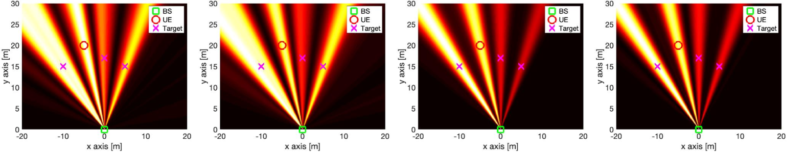
(a) BP: Digital-FDB        (b) BP: Analog-FDB        (c) BP: Digital-CPA        (d) BP: Analog-CPA

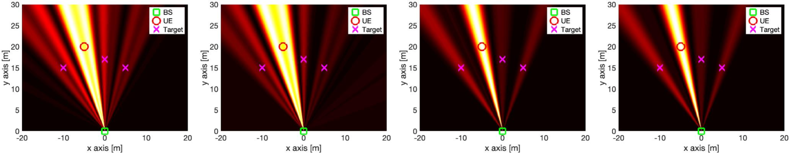
(e) MS: Digital-FDB        (f) MS: Analog-FDB        (g) MS: Digital-CPA        (h) MS: Analog-CPA

Figure 4: 2D beampatterns generated by different schemes, where the first row shows results for BP and the second row for MS: (a) Digital-FDB; (b) Analog-FDB; (c) Digital-CPA; (d) Analog-CPA; (e) Digital-FDB; (f) Analog-FDB; (g) Digital-CPA; and (h) Analog-CPA.

VI-B2 Analog Schemes

The complexity of the proposed AO-based analog beamforming schemes is determined by both the number of iterations and the complexity of each iteration. The detailed analysis is as follows:

• Analog-FDB: This scheme is addressed through AO, alternating between two SQP problems, each leading to inner quadratic subproblems classified as QCQP problems. The total complexity is expressed as $I_{\text{Ana}}^{\text{FDB-Pow}}C_{\text{Ana}}^{\text{FDB-Pow}}+I_{\text{Ana}}^{\text{FDB-Pha}}C_{\text{Ana}}^{\text{FDB-Pha}}$, where $I_{\text{Ana}}^{\text{FDB-Pow}}$ and $I_{\text{Ana}}^{\text{FDB-Pha}}$ represent the total iterations for the quadratic subproblems related to power allocation and phase optimization, respectively. The terms $C_{\text{Ana}}^{\text{FDB-Pow}}$ and $C_{\text{Ana}}^{\text{FDB-Pha}}$ refer to the complexity of solving these subproblems, respectively.

• Analog-CPA: The primary source of complexity in this scheme stems from the analog codebook construction, so the complexity of power allocation optimization after the codebook is obtained is not considered. The complexity for constructing $K+1$ codewords is given by $(K+1)I_{\text{Ana}}^{\text{CPA}}C_{\text{Ana}}^{\text{CPA}}$, where $I_{\text{Ana}}^{\text{CPA}}$ represents the total iterations for the inner closed-form updates of the adopted gradient projection method[44] when constructing a specific codeword. The terms $C_{\text{Ana}}^{\text{CPA}}$ denotes the complexity of computing the updates.

For clarity, the dominant per-iteration complexity of the proposed beamforming schemes is derived, simplified, and summarized in Table I. It is worth emphasizing that in high-frequency scenarios, such as millimeter-wave or even terahertz systems, the channel typically exhibits sparsity, leading to $K\ll N_{\text{B}}$. This sparsity allows us to exploit the optimal covariance matrix structure, thereby significantly reducing the computational complexity of the proposed digital beamforming approaches, which is now governed by an order of $K$.

VII Numerical Results

VII-A Scenarios

Unless specified otherwise, the simulation parameters are configured as follows: The BS is equipped with $N_{\text{B}}=16$ transmit/receive antennas, located at $\bm{p}_{\text{B}}=[0\text{ m},0\text{ m}]^{\mathsf{T}}$. The UE, with $N_{\text{U}}=16$ antennas, is positioned at $\bm{p}_{\text{U}}=[-5\text{ m},20\text{ m}]^{\mathsf{T}}$. There are $K=3$ targets, placed at $\bm{p}_{1}=[-10\text{ m},15\text{ m}]^{\mathsf{T}}$, $\bm{p}_{2}=[5\text{ m},15\text{ m}]^{\mathsf{T}}$, and $\bm{p}_{3}=[0\text{ m},17\text{ m}]^{\mathsf{T}}$. The transmit power is set at $P_{\text{B}}=-20\text{ dBm}$, with a carrier frequency of $f_{c}=28\text{ GHz}$ and a bandwidth of $W=120\text{ MHz}$. The system uses $M=1024$ subcarriers, with a noise figure of $F=10\text{ dB}$ and noise PSD $N_{0}=-173.855\text{ dBm/Hz}$. The simulation includes $L=16$ slots, each comprising $P=100$ pilot symbols, with a clock bias $\Delta t=1\;\mu\text{s}$ and a relative UE orientation of $\Delta\phi=(110/180)\pi$. The channel gains are generated using a standard free-space path loss model[12]. For the $k$-th path, the phases $\overline{\zeta}_{k}$ (for BP) and $\underline{\zeta}_{k}$ (for MS) are uniformly distributed over $[-\pi,\pi]$. In BP, the LOS channel gain is given by $\overline{\beta}_{0}=e^{\jmath\overline{\zeta}_{0}}\lambda/(4\pi\left\|\bm{p}_{\text{B}}-\bm{p}_{\text{U}}\right\|)$, while the non-line-of-sight (NLOS) channel gain is expressed as $\overline{\beta}_{k}=\overline{\sigma}_{\text{RCS},k}e^{\jmath\overline{\zeta}_{k}}\lambda/((4\pi)^{3/2}\left\|\bm{p}_{\text{U}}-\bm{p}_{k}\right\|\left\|\bm{p}_{k}-\bm{p}_{\text{B}}\right\|)$. For MS, the channel gain is expressed as $\underline{\beta}_{k}=\underline{\sigma}_{\text{RCS},k}e^{\jmath\overline{\zeta}_{k}}\lambda/((4\pi)^{3/2}\left\|\bm{p}_{k}-\bm{p}_{\text{B}}\right\|^{2})$. Here, $\overline{\sigma}_{\text{RCS},k}$ (for BP) and $\underline{\sigma}_{\text{RCS},k}$ (for MS) represent the radar cross section (RCS) of the $k$-th target. Specifically, $\underline{\sigma}_{\text{RCS},0}=10\text{ m}^{2}$, while $\overline{\sigma}_{\text{RCS},k}=\underline{\sigma}_{\text{RCS},k}=100\text{ m}^{2}$ ($k=1,\ldots,K$). The wavelength $\lambda$ is defined as $\lambda=c/f_{c}$, where $c$ is the speed of light.

VII-B Compared Schemes

We evaluate system performance using the proposed digital and analog beamforming approaches. Specifically, for the digital methods, we investigate the six schemes outlined in Section VI-B-1: FDB-WCRB, FDB-WBF, FDB-WCM, CPA-WCRB, CPA-WBF, and CPA-WCM. Additionally, we examine the fused BP-MS case described in Remark 1 within the digital-FDB-WCRB paradigm, which we refer to simply as “Fusion”. For the analog methods, we evaluate the two schemes outlined in Section VI-B-2: Analog-FDB and Analog-CPA.

(a) Digital FDB

(b) Digital CPA

(c) Analog FDB

(d) Analog CPA

Figure 5: Comparison of the tradeoff in terms of the square root of the CRB between BP and MS across various target numbers: (a) Digital FDB; (b) Digital CPA; (c) Analog FDB; and (d) Analog CPA.

VII-C Results and Discussion

VII-C1 Convergence

The proposed digital beamforming approaches (as well as Analog-CPA approach) are obtained either by SDP or QCQP and are solved via CVX with self-contained convergence. The proposed Analog-FDB approach is designed under the AO framework. Specifically, the convergence of objective value of $f(\bm{\rho},\bm{\Phi})$ is shown in Fig. 2. We observe that the objective value saturates within six iterations, validating the convergence of solving Analog-FDB via Algorithm 1.

VII-C2 Beampatterns

The core rationale behind the adopted Analog-CPA approach is to replicate the digital codebook through an analog equivalent. To illustrate this, Fig. 3 compares the beampatterns of various digital-analog pairs. As shown, the dashed lines represent the beampatterns of the generated analog codewords and closely match the solid lines, which represent those of the original digital codewords. This strong alignment confirms that the analog codebook construction method[44], effectively preserves the spatial signatures, thereby substantiating the effectiveness of the Analog-CPA scheme, which we further elaborate on subsequently.

In Fig. 4, we present the 2D beampatterns for various approaches across different scenarios, illustrating the spatial behavior and characteristics of the proposed beamforming techniques under extreme conditions. This comparison provides insights into the performance tradeoff between BP and MS, which we will further analyze in detail later. The top row shows results for BP ($\alpha=1$), while the bottom row corresponds to MS ($\alpha=0$). Within each row, the outcomes for the Digital-FDB, Analog-FDB, Digital-CPA, and Analog-CPA schemes are shown sequentially from left to right.

In general, for BP, all schemes direct strong beams toward the UE, with variations in power allocated to beams aimed at the targets. This occurs because the BS serves as the primary anchor in BP, while the targets act as secondary anchors, with their positions being estimated concurrently. The information provided about the UE’s position varies based on relative locations, which leads to a power adjustment across beams illuminating the targets to maximize UE positioning accuracy. In MS, accurate positioning of both the targets and the UE is crucial for optimal performance. Due to the UE’s relatively small RCS, stronger beams are consistently directed toward it in all schemes to maintain balanced positioning accuracy across all targets.

Additionally, beams generated by FDB-based approaches are broader compared to those from CPA-based approaches. This is due to a larger design degrees-of-freedoms in FDB-based methods, which enable the synthesis of beams directed around the targets from a predetermined codebook, thus enhancing spatial information extraction for superior BP and/or MS performance. Conversely, CPA-based approaches, constrained by limited design DOFs due to their power allocation nature, can only transmit beams along predetermined directions. Furthermore, both the digital approaches and their analog counterparts show alignment in their beampatterns, demonstrating the potential efficacy of the proposed analog beamforming approaches.

(a) Holistic comparison

(b) Fusion

Figure 6: Comparison of the tradeoff in terms of the square root of the CRB between BP and MS across various schemes: (1) Holistic perspective; (2) Closer examination of the fusion scenario.

VII-C3 Tradeoff between BP and MS

In Fig. 5, we examine the performance tradeoff between BP and MS, measured by the square root of the CRB, across different target numbers and under various schemes. Target numbers range from one to three, as at least one target is required for feasible BP in the considered setting [23]. All curves reveal the fundamental tradeoff between BP and MS. For digital schemes, we compare results across three paradigms: WCRB, WBF, and WCM. Among these, the WCRB approach demonstrates the most favorable bistatic-monostatic performance tradeoff, outperforming the weighted-sum mismatch approaches (WBF and WCM), as the latter exhibit weak Pareto frontier. Notably, within both Digital-FDB and Digital-CPA approaches, schemes based on WCM consistently show a superior bistatic-monostatic performance tradeoff compared to those based on WBF, with results nearly reaching the weak Pareto frontier[38]. Additionally, in the Digital-FDB scheme, the performance gap between WBF and WCM becomes more pronounced as the target number increases. This observation suggests that approximating the covariance matrix directly preserves the desired spatial characteristics of the transmitted signal more effectively than beamformer approximation, as the FIM elements are determined directly by the covariance matrix. This insight supports the motivation for adopting the WCM paradigm in developing analog beamforming schemes.

It is also worth noting an interesting trend: as the number of targets increases, BP CRB decreases, while MS CRB increases, causing the tradeoff curves to shift upward and to the left with increasing $K$. This can be attributed to each resolvable target enhancing the position-related information of the UE[23], thus improving BP performance. In contrast, a higher target number imposes a heavier load on MS due to the limited, fixed spatial DOFs that must be allocated across multiple targets, leading to reduced overall MS performance.

In Fig. 6, we compare the performance tradeoff between BP and MS across various schemes for the case when $K=3$. Additionally, the Fusion scheme is presented to illustrate the advantages of information exchange between the BS and UE, enabling improved joint BP and MS performance. Fig. 6(a) offers a comprehensive comparison across all approaches, where we observe a noticeable performance reduction from the proposed digital approaches to their analog counterparts. This reduction is attributed to the limited design DOFs in analog approaches, constrained by unit-modulus requirements necessary to maintain analog characteristics. Furthermore, within both digital and analog categories, the FDB schemes significantly outperform CPA in the bistatic-monostatic performance tradeoff, due to their higher optimization DOF. The Fusion scheme surpasses all other approaches by fully leveraging shared tasks between BP and MS, highlighting the considerable benefits of this mutualistic mechanism for enhancing joint BP and MS performance. Finally, we note that the Fusion scheme minimizes the tradeoff between BP and MS to such an extent that Fig. 6(a) displays it as nearly a single point. However, as shown in Fig. 6(b), even when minimized, a fundamental tradeoff between BP and MS persists, which becomes apparent upon closer inspection.

VIII Conclusion

In this study, we investigated the joint optimization of BP and MS within a MIMO OFDM framework, proposing innovative beamforming strategies that enable flexible tradeoff between BP and MS performance. We derived CRBs for both BP and MS, targeting two primary objectives: allowing user equipment to estimate its position while accounting for clock bias and orientation mismatches, and enabling the BS to localize passive targets. This led to a multi-objective optimization problem for beamforming. We analyzed digital schemes using weighted-sum CRB and mismatch minimization approaches, evaluating their performance under FDB and CPA. To enhance hardware efficiency, we developed analog FDB and CPA strategies based on covariance matrix mismatch minimization. Our numerical results demonstrate the effectiveness of the proposed designs, highlighting the advantages of minimizing covariance matrix mismatch and underscoring the benefits of information fusion between BP and MS for practical system implementation. There are several interesting avenues for future research, including: 1) considering the uncertainty in UE/target positions, 2) examining different visibility conditions between BP and MS in terms of targets, and 3) analyzing targets in the near field of BS/UE.

Appendix A Fundamentals of the SQP Framework

According to [43], the SQP algorithm is an iterative approach for addressing nonlinear optimization problems, formulated as

$$\mathop{\min}\limits_{\bm{x}}\;\;\; f\left(\bm{x}\right)$$ (28a)

$${\rm{s.t.}}\;\;\; g_{i}\left(\bm{x}\right)=0,\quad i=1,\ldots,m,$$ (28b)

$$h_{j}\left(\bm{x}\right)=0,\quad j=1,\ldots,p,$$ (28c)

where $f(\bm{x})$ represents the objective function, while $g_{i}(\bm{x})$ and $h_{j}(\bm{x})$ denote the equality and inequality constraints, respectively.

The primary components integral to understanding the SQP workflow are as follows.

1. Lagrangian Function: Defined as $\mathcal{L}(\bm{x},\bm{\lambda},\bm{\mu})=f(\bm{x})+\sum_{i=1}^{m}\lambda_{i}g_{i}(\bm{x})+\sum_{j=1}^{p}\mu_{j}h_{j}(\bm{x}),$ where $\bm{\lambda}=[\lambda_{1},\ldots,\lambda_{m}]^{\mathsf{T}}$ and $\bm{\mu}=[\mu_{1},\ldots,\mu_{p}]^{\mathsf{T}}$ are Lagrange multipliers for equality and inequality constraints.

2. Quadratic Subproblem: At the $k$-th iteration, SQP solves a quadratic approximation of the Lagrangian around $\bm{x}_{k}$ under linearized constraints, expressed as

   $$\mathop{\min}\limits_{\bm{p}}\;\;\; \nabla f\left(\bm{x}_{k}\right)^{\mathsf{T}}\bm{p}+\frac{1}{2}\bm{p}^{\mathsf{T}}\nabla^{2}\mathcal{L}\left(\bm{x}_{k},\bm{\lambda}_{k},\bm{\mu}_{k}\right)\bm{p}$$ (29a)

   $${\rm{s.t.}}\;\;\; \nabla g_{i}\left(\bm{x}_{k}\right)^{\mathsf{T}}\bm{p}+g_{i}\left(\bm{x}_{k}\right)=0,\quad\forall i,$$ (29b)

   $$\nabla h_{j}\left(\bm{x}_{k}\right)^{\mathsf{T}}\bm{p}+h_{j}\left(\bm{x}_{k}\right)\leq 0,\quad\forall j,$$ (29c)

   where $\nabla f(\bm{x}_{k})$ and $\nabla^{2}\mathcal{L}(\bm{x}_{k},\bm{\lambda}_{k},\bm{\mu}_{k})$ are the gradient vector and Hessian matrix of $f(\bm{x})$ evaluated at $\bm{x}=\bm{x}_{0}$.

3. Merit Function: To ensure simultaneous improvement in the objective and constraints, a merit function is defined as $\phi(x,\lambda)=f(x)+\alpha(\sum_{i=1}^{m}|g_{i}(x)|+\sum_{j=1}^{p}\max(0,h_{j}(x)))$ with $\alpha$ as a penalty parameter.

The SQP algorithm follows these steps.

1. Initialization: Choose an initial guess $\bm{x}_{0}$ and set initial multipliers $\bm{\lambda}_{0}$ and $\bm{\mu}_{0}$.

2. Quadratic Subproblem: At the $k$-th iteration, solve (29) to determine the search direction $\bm{p}_{k}$.

3. Line Search or Trust Region: Select a step size $\overline{\beta}_{k}$ that ensures a sufficient decrease in the merit function.

4. Update: Set $\bm{x}_{k+1}=\bm{x}_{k}+\overline{\beta}_{k}\bm{p}_{k}$ and update $\bm{\lambda}_{k}$ and $\bm{\mu}_{k}$.

5. Check: Repeat until the Karush–Kuhn–Tucker conditions are approximately met.

References

- [1] F. Liu et al., “Joint radar and communication design: Applications, state-of-the-art, and the road ahead,” IEEE Transactions on Communications, vol. 68, no. 6, pp. 3834–3862, 2020.
- [2] ——, “Integrated sensing and communications: Toward dual-functional wireless networks for 6G and beyond,” IEEE Journal on Selected Areas in Communications, vol. 40, no. 6, pp. 1728–1767, 2022.
- [3] J. A. Zhang et al., “An overview of signal processing techniques for joint communication and radar sensing,” IEEE Journal of Selected Topics in Signal Processing, vol. 15, no. 6, pp. 1295–1315, 2021.
- [4] A. Liu et al., “A survey on fundamental limits of integrated sensing and communication,” IEEE Communications Surveys & Tutorials, vol. 24, no. 2, pp. 994–1034, 2022.
- [5] S. Lu et al., “Integrated sensing and communications: Recent advances and ten open challenges,” IEEE Internet of Things Journal, vol. 11, no. 11, pp. 19 094–19 120, 2024.
- [6] N. González-Prelcic et al., “The integrated sensing and communication revolution for 6G: Vision, techniques, and applications,” Proceedings of the IEEE, vol. 112, no. 7, pp. 676–723, 2024.
- [7] H. Chen et al., “A tutorial on terahertz-band localization for 6G communication systems,” IEEE Communications Surveys & Tutorials, vol. 24, no. 3, pp. 1780–1815, 2022.
- [8] A. Behravan et al., “Positioning and sensing in 6G: Gaps, challenges, and opportunities,” IEEE Vehicular Technology Magazine, vol. 18, no. 1, pp. 40–48, 2022.
- [9] H. Sallouha et al., “On the ground and in the sky: A tutorial on radio localization in ground-air-space networks,” IEEE Communications Surveys & Tutorials, pp. 1–1, 2024.
- [10] L. Italiano et al., “A tutorial on 5G positioning,” IEEE Communications Surveys & Tutorials, pp. 1–1, 2024.
- [11] Y. Ge et al., “Integrated monostatic and bistatic mmWave sensing,” in GLOBECOM 2023 - 2023 IEEE Global Communications Conference, 2023, pp. 3897–3903.
- [12] H. Wymeersch et al., “Radio localization and sensing—Part I: Fundamentals,” IEEE Communications Letters, vol. 26, no. 12, pp. 2816–2820, 2022.
- [13] H.-S. Cha et al., “5G NR positioning enhancements in 3GPP Release-18,” arXiv preprint arXiv:2401.17594, 2024.
- [14] K. E. Olsen et al., “Bridging the gap between civilian and military passive radar,” IEEE Aerospace and Electronic Systems Magazine, vol. 32, no. 2, pp. 4–12, 2017.
- [15] F. Liu et al., “Seventy years of radar and communications: The road from separation to integration,” IEEE Signal Processing Magazine, vol. 40, no. 5, pp. 106–121, 2023.
- [16] F. Dong et al., “Sensing as a service in 6G perceptive networks: A unified framework for ISAC resource allocation,” IEEE Transactions on Wireless Communications, vol. 22, no. 5, pp. 3522–3536, 2023.
- [17] L. Xie et al., “Collaborative sensing in perceptive mobile networks: Opportunities and challenges,” IEEE Wireless Communications, vol. 30, no. 1, pp. 16–23, 2023.
- [18] F. Liu et al., “Radar-assisted predictive beamforming for vehicular links: Communication served by sensing,” IEEE Transactions on Wireless Communications, vol. 19, no. 11, pp. 7704–7719, 2020.
- [19] W. Yuan et al., “Bayesian predictive beamforming for vehicular networks: A low-overhead joint radar-communication approach,” IEEE Transactions on Wireless Communications, vol. 20, no. 3, pp. 1442–1456, 2021.
- [20] A. Kaushik et al., “Toward integrated sensing and communications for 6G: Key enabling technologies, standardization, and challenges,” IEEE Communications Standards Magazine, vol. 8, no. 2, pp. 52–59, 2024.
- [21] H. Chen et al., “RISs and sidelink communications in smart cities: The key to seamless localization and sensing,” IEEE Communications Magazine, vol. 61, no. 8, pp. 140–146, 2023.
- [22] A. Shahmansoori et al., “Position and orientation estimation through millimeter-wave MIMO in 5G systems,” IEEE Transactions on Wireless Communications, vol. 17, no. 3, pp. 1822–1835, 2018.
- [23] R. Mendrzik et al., “Harnessing NLOS components for position and orientation estimation in 5G millimeter wave mimo,” IEEE Transactions on Wireless Communications, vol. 18, no. 1, pp. 93–107, 2019.
- [24] Y. Ge et al., “A computationally efficient EK-PMBM filter for bistatic mmWave radio SLAM,” IEEE Journal on Selected Areas in Communications, vol. 40, no. 7, pp. 2179–2192, 2022.
- [25] M. A. Nazari et al., “MmWave 6D radio localization with a snapshot observation from a single BS,” IEEE Transactions on Vehicular Technology, vol. 72, no. 7, pp. 8914–8928, 2023.
- [26] F. Liu et al., “MU-MIMO communications with MIMO radar: From co-existence to joint transmission,” IEEE Trans. Wireless Commun., vol. 17, no. 4, pp. 2755–2770, 2018.
- [27] ——, “Toward dual-functional radar-communication systems: Optimal waveform design,” IEEE Trans. Signal Process., vol. 66, no. 16, pp. 4264–4279, 2018.
- [28] X. Liu et al., “Joint transmit beamforming for multiuser MIMO communications and MIMO radar,” IEEE Trans. Signal Process., vol. 68, pp. 3929–3944, 2020.
- [29] ——, “Transmit design for joint MIMO radar and multiuser communications with transmit covariance constraint,” IEEE J. Sel. Areas Commun., vol. 40, no. 6, pp. 1932–1950, 2022.
- [30] F. Liu et al., “Cramér-Rao bound optimization for joint radar-communication beamforming,” IEEE Trans. Signal Process., vol. 70, pp. 240–253, 2022.
- [31] X. Song et al., “Intelligent reflecting surface enabled sensing: Cramér-Rao bound optimization,” IEEE Transactions on Signal Processing, vol. 71, pp. 2011–2026, 2023.
- [32] L. Chen et al., “Generalized transceiver beamforming for DFRC with MIMO radar and MU-MIMO communication,” IEEE J. Sel. Areas Commun., vol. 40, no. 6, pp. 1795–1808, 2022.
- [33] R. Liu et al., “Joint waveform and filter designs for STAP-SLP-based MIMO-DFRC systems,” IEEE J. Sel. Areas Commun., vol. 40, no. 6, pp. 1918–1931, 2022.
- [34] Y. Zhang et al., “Robust transceiver design for covert integrated sensing and communications with imperfect CSI,” IEEE Transactions on Communications, pp. 1–1, 2024.
- [35] M. F. Keskin et al., “Optimal spatial signal design for mmwave positioning under imperfect synchronization,” IEEE Transactions on Vehicular Technology, vol. 71, no. 5, pp. 5558–5563, 2022.
- [36] A. Fascista et al., “RIS-aided joint localization and synchronization with a single-antenna receiver: Beamforming design and low-complexity estimation,” IEEE Journal of Selected Topics in Signal Processing, vol. 16, no. 5, pp. 1141–1156, 2022.
- [37] S. H. Talisa et al., “Benefits of digital phased array radars,” Proceedings of the IEEE, vol. 104, no. 3, pp. 530–543, 2016.
- [38] M. Ehrgott, Multicriteria optimization. Springer Science & Business Media, 2005, vol. 491.
- [39] Z.-Q. Luo et al., “Semidefinite relaxation of quadratic optimization problems,” IEEE Signal Processing Magazine, vol. 27, no. 3, pp. 20–34, 2010.
- [40] J. Li et al., “Range compression and waveform optimization for MIMO radar: A CramÉr–Rao bound based study,” IEEE Transactions on Signal Processing, vol. 56, no. 1, pp. 218–232, 2008.
- [41] L. You et al., “Integrated communications and localization for massive MIMO LEO satellite systems,” IEEE Transactions on Wireless Communications, vol. 23, no. 9, pp. 11 061–11 075, 2024.
- [42] C. Fortin et al., “The trust region subproblem and semidefinite programming,” Optimization methods and software, vol. 19, no. 1, pp. 41–67, 2004.
- [43] J. Nocedal et al., Numerical optimization. Springer Science & Business Media, 2006.
- [44] J. Tranter et al., “Fast unit-modulus least squares with applications in beamforming,” IEEE Transactions on Signal Processing, vol. 65, no. 11, pp. 2875–2887, 2017.
- [45] S. Boyd et al., Convex optimization. Cambridge university press, 2004.