Cosmic dynamics and observational constraints in $f(Q)$ gravity with affine equation of state

Abstract

In this study, we explore the cosmological implications of $f(Q)$ gravity with an affine equation of state (EoS). We study the impact of affine EoS on the cosmic evolution in model and derive the functional form of $f(Q)$ gravity realizing this kind of scenario. We show that the non-metricity scalar may describe the unified scenario in which the universe transits from the decelerated expansion into the accelerated expansion. The model parameters are constrained through the Bayesian analysis based on $\chi^{2}$ minimization technique with the observational data of the cosmic chronometer and supernovae type Ia. The cosmic dynamics based on constrained parameters describe the observable universe evolution. The present day values of the cosmological parameters along with the current age of the universe are compatible with the observations.

Keywords: Dark fluid; EoS; Unified scenario; Observations; Non-metricity

1 Introduction

The validation of accelerated cosmic expansion signifies the beginning of a new era in cosmological study. This phenomena was initially noticed by while observing type Ia supernovae [1, 2]. Subsequently, the universe’s expansion has been confirmed by numerous observations [3, 4, 5]. An unusual fluid/field with negative pressure is a cause of the universe’s late-time accelerated expansion [6, 7]. This kind of fluid/field has been termed as the ‘dark energy’ whose exact nature remains mysterious [8, 6]. In other words, the dark energy, theoretically modeled to generate negative pressure has been believed to be responsible for the universe’s accelerated expansion [9, 10, 11, 12, 13, 14]. The most widely accepted model of universe is the $\Lambda$ cold dark matter ($\Lambda$CDM) model. In this model, the dark energy is described by the constant vacuum energy density which is visualized as the cosmological constant in the model [6, 7]. This model is consistent with the observations, however, it faces several challenges [15, 6, 7, 13]. The enormous difference between the theoretically calculated and observational required values of vacuum energy corresponding to cosmological constant causes the issue of fine tuning [6, 7]. In order to resolve the challenges of $\Lambda$CDM model, the alternative approaches where the dark energy is a dynamical one is generally explored in the cosmological modeling.

The issues related to the cosmic acceleration have been explored in dark energy models of the General relativity (GR) as well as the modified theories of gravity. Finding a modification of GR that allows cosmic acceleration without including any exotic components is an interesting option. One of the most well-known ideas to explain the dark contents of the universe is described by the $f(R)$ gravity [16]. This theory is a modification of General Relativity, where $R$ is the Ricci Scalar. Different theories of gravity have been explored to describe issues of dark energy and dark matter, see [17, 18, 19, 20, 10, 11, 21, 22, 23, 24, 25, 26, 27, 28, 29, 30, 31, 32] and references therein.

In the context of modified gravity theories, Jimenez et al. [33] proposed a gravity theory based on non-metricity and is termed as $f(Q)$ gravity. This theory is based on an approach which considers a variation of the symmetric teleparallel equivalence to General Relativity, here $Q$ is a non-metricity scalar. The studies [13, 34], suggest that the $f(Q)$ theory is one of the intriguing alternative gravity interpretations for explaining the cosmological evolution. Lazkoz et al. [35] investigated the accelerated expansion of the universe in context of its consistency with observational data. The exact cosmic solutions that are both anisotropic and isotropic were studied by Esposito et al.[36]. Harko et al. [37] developed a class of $f(Q)$ theories where $Q$ is non-minimally associated with the matter Lagrangian. In connection with the $f(Q)$ gravity theory, numerous further studies [33, 34, 35, 36, 37, 38, 39, 40, 41, 42, 43, 44, 45, 46, 47, 48, 49, 50, 51, 52, 53, 54, 55] suggest that the theory may have interesting cosmological and astrophysical implications, for review see [14].

In this paper, we study the implications of $f(Q)$ gravity with the dark fluid satisfying affine equation of state. We search for an answer whether the $f(Q)$ gravity may have fluid description or not? In particular, for an affine equation of state of dark fluid, we derive the functional formulation of $f(Q)$ gravity. The issue of observational compatibility of model may describe the observational constraints on model parameters. The dark fluid have been studied in the isotropic and anisotropic spacetime with the General relativity framework [56, 57, 58, 59, 60, 61, 62, 63, 64, 65, 66, 67, 68, 69, 70, 71]. The affine equation of state describes the hydro-dynamically stable as well as unstable fluid propagation. The speed of sound remains constant for the fluid. The stable dark energy evolution may be visualized with the fluid satisfying affine equation of state given by $p_{d}=\alpha\rho_{d}-\rho_{0}$, where $\alpha$ and $\rho_{0}$ are constants. The classical stability criterion constrains $0\leq\alpha\leq 1$. In a non-conservative theory, this kind of EoS may naturally arise near the bouncing instant of bouncing universe [66, 68]. The low energy limits of this kind of EoS may have the $\Lambda$CDM limit [60]. Based on these peculiar properties, we aim to study the cosmological implications of this fluid in $f(Q)$ gravity to describes the fluid interpretation of this modified gravity.

This paper is organized in the following way: An overview of the mathematical aspects of $f(Q)$ gravity in a flat FLRW background has been given in section (2). In Section (3), we obtain the cosmological solutions of the affine EoS model with $f(Q)$ gravity. In Section (4), the Bayesian statistical tools are used to investigate the compatibility of cosmological solution with the cosmic chronometer (CC) and supernovae type Ia (Pantheon) datasets. The cosmological dynamics based on the parameters such as the deceleration parameter, pressure, energy density, cosmographic parameter and the age of universe are studied in section (5). The conclusion with summary of results are given in Section (6).

2 An overview of $f(Q)$ gravity

The $f(Q)$ gravity is based on the non-metricity scalar $Q$. The $f(Q)$ gravity is characterized by the following action [33]

$${}S=\int\sqrt{-g}\,d^{4}x\left[-\frac{1}{2}f(Q)+\mathcal{L}_{m}\right].$$ (1)

Here, $f(Q)$ represents an arbitrary function of the nonmetricity scalar $Q$. The symbol $g$ denotes metric tensor’s determinant $g_{ab}$ and the Lagrangian density for matter is symbolized by $\mathcal{L}_{m}$. The quantity $Q$ can be characterized by two distinct traces as

$${}Q_{\sigma}=Q_{\sigma}^{\phantom{\sigma}a}a_{\phantom{a}},\quad\tilde{Q}_{\sigma}=Q^{a\phantom{\mu}}_{\phantom{\mu}\sigma a}.$$ (2)

Furthermore, the non-metricity scalar $(Q)$ may be expressed by the contraction of above tensors and may be defined as:

$${}Q=-Q_{\sigma ab}P^{\sigma ab},$$ (3)

Additionally, the superpotential tensor (which is a conjugate of non-metricity) can be introduced as:

$${}4P^{\sigma}_{\phantom{\sigma}ab}=2Q_{(a\phantom{\sigma}b)}^{\phantom{\mu}\sigma}-\tilde{Q}^{\sigma}g_{ab}-Q^{\sigma}_{\phantom{\sigma}ab}-Q^{\sigma}g_{ab}-\delta^{\sigma}_{(a}Q_{b)}^{\phantom{\nu)}},$$ (4)

The field equation may obtained by varying the action (1) with respect to the metric and are expressed as [33]

$${}\frac{2}{\sqrt{-g}}\nabla_{\sigma}\left(\sqrt{-g}f_{Q}P^{\sigma}_{ab}\right)+\frac{1}{2}g_{ab}f+f_{Q}\left(P_{a\sigma\beta}Q^{\sigma\beta}_{\phantom{\sigma\beta}b}-2Q_{\sigma\beta a}P^{\sigma\beta}_{\phantom{\sigma\beta}b}\right)=T_{ab},$$ (5)

where, $f_{Q}=\frac{df(Q)}{dQ}$ and energy-momentum tensor may be written as $T_{\mu\nu}=-\frac{2}{\sqrt{-g}}\frac{\delta(\sqrt{-g}\mathcal{L}_{m})}{\delta g^{\mu\nu}}$. We are assuming the unit system where $8\pi G=c=1$.
The energy-momentum tensor $T_{ab}$ might also be written for perfect fluid as $T_{ab}=pg_{ab}+(p+\rho)u_{a}u_{b}$. The perfect fluid’s isotropic pressure and energy density are denoted as $p$ and $\rho$ respectively. The fluid’s $4$-velocity $u_{a}$ satisfies the normalization condition $u_{a}u^{a}=-1$.
Here, we proceed with the framework of spatially flat FLRW spacetime, defined by

$${}ds^{2}=a^{2}(t)\left(dx^{2}+dy^{2}+dz^{2}\right)-dt^{2},$$ (6)

Under these conditions, the non-metricity scalar $Q$ may be described as $Q=6H^{2}$, where $H\equiv\frac{\dot{a}}{a}$ symbolizes the Hubble parameter and $a(t)$ is the scale factor. The overhead dot has been used to indicate the derivative with respect to cosmic time $t$. For the metric (6), the Friedmann equations can be expressed as follows [72]:

$$H^{2}=\frac{1}{6f_{Q}}\left(\rho+\frac{f}{2}\right),\quad\dot{H}+3H^{2}+\frac{H\dot{f}_{Q}}{f_{Q}}=\frac{1}{2f_{Q}}\left(\frac{f}{2}-p\right)$$ (7)

If $f(Q)$ is assumed to be $f(Q)=Q$ [72], one may obtain the standard field equations of the General Relativity. By considering $f(Q)=Q+F(Q)$, the above field equations (7) may also be expressed as

$$3H^{2}=\rho+\frac{F}{2}-QF_{Q},\quad\dot{H}(2QF_{QQ}+F_{Q}+1)+\frac{1}{4}\left(2QF_{Q}-F+Q\right)=-\frac{p}{2}$$ (8)

The Eqs (8) may be seen as modifications of General Relativity equations, incorporating an additional term that arises from the non-metricity ($Q$) of space-time. This term may exhibit a characteristics similar to a fluid component associated with dark sector of the fluid component of universe, i.e. $p_{Q}=p_{d}$ and $\rho_{Q}=\rho_{d}$. Consequently, using Eqs. (8), we may write

$$3H^{2}=(\rho+\rho_{d}),\quad 2\dot{H}+3H^{2}=-(p+p_{d}),$$ (9)

The pressure and density contributions to dark energy may be represented by $p_{d}$ and $\rho_{d}$ respectively, which may be caused by the non-metricity of spacetime. We define

$${}\rho_{d}=\frac{F}{2}-QF_{Q},\quad p_{d}=2\dot{H}(2QF_{QQ}+F_{Q})-\rho_{d}.$$ (10)

These equations may be used to obtain the solution of system and thus the resulting Hubble parameter may be used for the identification of the cosmic evolution in model. We proceed to setup the unified scenario of universe evolution in this $f(Q)$ model, where the transiting universe evolution may be described by the non-metricity scalar.

3 The cosmological solutions with the affine equation of state in $f(Q)$ model

We proceed by taking the fluid which may represent the hydro-dynamically dark energy. The fluid has been assumed to have form [56, 61, 71]

$$p_{d}=\alpha\rho_{d}-\rho_{0}$$ (11)

where $\alpha$ and $\rho_{0}$ are some constants. For $\rho_{0}=0$, one may have the usual relation of EoS as $p_{d}=\omega\rho_{d}$ for $\alpha=\omega$. The parameter $\alpha$ may be visualized as constant speed of sound and the classical stability criterion constrains $0\leq\alpha\leq 1$. The causality and stability issues are important as far as the physical acceptability of a cosmological model is concerned [73, 74]. In a given medium, the sound speed describes the propagation speed of the acoustic (pressure) waves. The behavior of squared sound speed may be described by ${c_{s}}^{2}=\frac{\partial{p_{d}}}{\partial{\rho_{d}}}$. The uncontrolled growth of energy density perturbations may be prevented by ${c_{s}}^{2}>0$. The prevention of causality violation would lead to ${c_{s}}^{2}<1$. In the subsequent sections, we consider the cases where $\rho=0$ and $\rho\neq 0$ in the Eqs. (9) to write the cosmological solutions. With these assumptions, we check the impact of $\rho$ term in cosmic dynamics yielded in these different models. The energy conservation equation for the fluid may be written as

$$\dot{\rho}_{d}+3H(\rho_{d}+p_{d})=0$$ (12)

One may observe that for $\rho_{d}<\frac{\rho_{0}}{1+\alpha}$, one may have the phantom evolution of dark energy in model. For $\rho_{d}=\frac{\rho_{0}}{1+\alpha}$, the dynamics of constant vacuum energy may be visualized. For $\rho_{d}>\frac{\rho_{0}}{1+\alpha}$, the null energy condition will be satisfied in model, as a consequence the fluid distribution may either have the quintessence domination or the normal matter (composed of matter or radiation) domination. Based on these possible evolution dynamics, we probe the universe evolution under influence of dark fluid (given by Eq. (11)) in $f(Q)$ model.

3.1 Model I

For the case $\rho=0$ in Eqs. (9) and (10), we may obtain $\rho_{d}=3H^{2}$ and it would lead to $F(Q)=-Q+C\sqrt{Q}$, where $C$ is an integration constant. The form of $f(Q)$ function may be written as

$$f(Q)=C\sqrt{Q}$$ (13)

The above functional form of $f(Q)$ may describe the evolution with dark fluid having form (11). The continuity equation (12) may lead to the form of $\rho_{d}$ depending on the scale factor as

$${}\rho_{d}=\frac{\rho_{0}+(1+z)^{3(\alpha+1)}}{\alpha+1}$$ (14)

This Eq. (14) would yield the Hubble parameter for this case as

$${}H(z)=H_{0}\sqrt{\frac{(1+z)^{3(1+\alpha)}+\rho_{0}}{\rho_{0}+1}},\quad\text{where,}\quad H_{0}=\sqrt{\frac{\rho_{0}+1}{3(1+\alpha)}}$$ (15)

The above Hubble parameter may describe the cosmic evolution in the $f(Q)$ gravity yielded by the fluid following affine equation of state (11). The observational constraints on the model parameters $\alpha,\rho_{0}$ and $H_{0}$ may describe the observational compatibility of model along with the validity of causality principle in this model.

3.2 Model II

In the present case, we take $\rho\neq 0$ in equation (9) and assume that $\rho$ is the energy density of pressure-less matter satisfying $p=0$. As a consequence, $\rho=\rho_{m0}a^{-3}$, where $\rho_{m0}$ is energy density of matter at $z=0$. In this case, $\rho_{d}$ may be the energy density of dark energy. In this case, the Hubble parameter may be obtained as

$${}H(z)=H_{0}\sqrt{(1+z)^{3}\left[\Omega_{m0}+\left(\frac{1-\Omega_{m0}}{\rho_{0}+1}\right)(1+z)^{3\alpha}\right]+\left(\frac{1-\Omega_{m0}}{\rho_{0}+1}\right)\rho_{0}}$$ (16)

where $\Omega_{m0}=\frac{\rho_{m0}}{3H_{0}^{2}}$. This Hubble parameter may describe the cosmic dynamics in $f(Q)$ gravity where the fluids are composed of the pressure-less matter and dark energy satisfying $p=0$ and $p_{d}=\alpha\rho_{d}-\rho_{0}$ respectively.

4 Observational constraints and results

Within this part, we focus on describing the data sets that are utilized to analyze the models. We also explain constraints on Model I(15) and Model II(16)’s model parameters. In other words, the consistency of the Hubble parameter (15) and (16) with the data sets given by the Cosmic Chronometer (CC) and combined data that consists of Pantheon and CC are used in the MCMC analysis. We constrain the parameters ($H_{0}$, $\alpha$, $\rho_{0}$ and $\Omega_{m0}$) using the $\chi^{2}$ minimization method and the MCMC method is implemented with the emcee Python library [75].

4.1 The Cosmic chronometer data

The model parameters ($H_{0}$, $\alpha$, $\rho_{0}$ and $\Omega_{m0}$) are constrained using Cosmic Chronometer data consisting of $31$ data points in the red-shift range of $0.07\leq z\leq 1.965$ are collected using the differential ages of galaxies approach [76, 77]. The cosmic chronometer observations’s fundamental principle (introduced by Jimenez and Loeb [78]) introduces a relationship between red-shift $(z)$, cosmic time $t$, and the Hubble parameter $H(z)$ as $H(z)=\frac{-1}{(1+z)}\frac{dz}{dt}$. By minimizing the $\chi^{2}$ function, we determine the model parameters’s central values with $1\sigma$ errors in the emcee[75] package. For the Cosmic chronometer data, the $\chi^{2}$ function may be represented as [71, 79, 80, 81]:

$${}\chi^{2}_{CC}(\theta)=\sum_{i=1}^{31}\frac{[H_{th}(\theta,z_{i})-H_{obs}(z_{i})]^{2}}{\sigma^{2}_{i}}.$$ (17)

Here, $H_{th}$ is used to indicate the theoretical values of the Hubble parameter, the observed values are indicated by $H_{obs}(z_{i})$ and the notation $\sigma_{i}$ indicates the standard deviation for each $H_{obs}(z_{i})$ observed value.
The emcee [75] results yield the median values of posterior distributions for the model parameters. Tables (1) and (2) provide summaries of these values for Model I and Model II, respectively. The error bars of the CC points alongside the best fit Hubble parameter curve derived from equation (15), (16) are illustrated in figure $(\ref{fig:1})$.

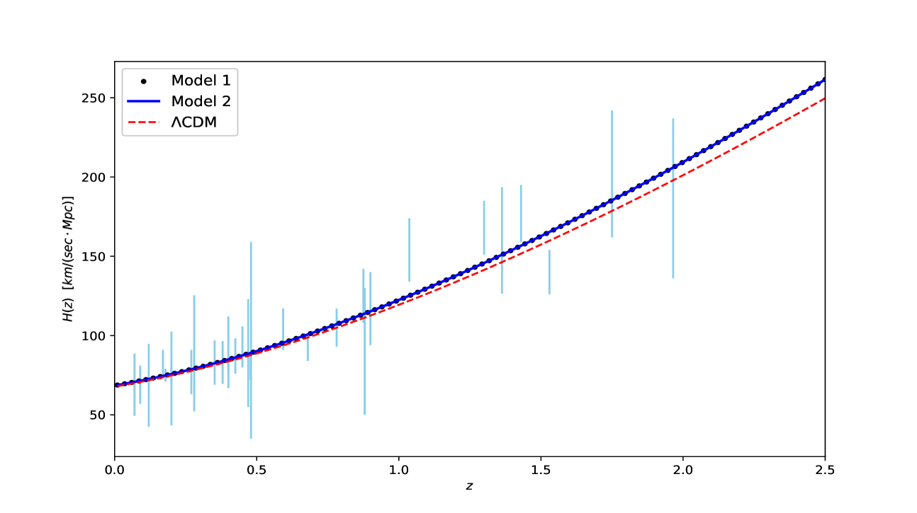
Figure 1: In comparison to the $\Lambda CDM$ model, the best fit Hubble parameter curves versus $\mathit{z}$.

It may observed that the cosmic dynamics of the Model I and II are deviating from the $\Lambda$CDM model in the past where $z>1$. The transition redshift however remains close to the $\Lambda$CDM model. It is worthwhile to observe from these results that the Model I may describe the transiting universe evolution from the decelerated expansion into the accelerated expansion and the even with the consideration of pressure-less matter in Model II, the cosmic dynamics remains identical as that of the Model I.

4.2 The Pantheon data

The Pantheon data is composed of supernovae type Ia (SNIa) observations identified in the low and high red-shift ranges [82]. This dataset includes $1048$ data points within the redshift interval $0.01\leq z\leq 2.26$. For the purpose of examining cosmic expansion of the observable universe, SNIa are widely adopted as the standard candles with their theoretical apparent magnitude $m_{th}(z)$ are given by:

$${}m_{th}(z)=M+5\log_{10}\left[\frac{d_{L}(z)}{1Mpc}\right]+25,$$ (18)

where, $M$ is absolute magnitude, $c$ denotes the speed of light, $z$ represents the SNIa red-shift in the CMB rest frame and $d_{L}(z)=c(1+z)\int_{0}^{z}\frac{dz^{\prime}}{H(z^{\prime})}$ is the luminosity distance. The luminosity distance $d_{L}(z)$ is typically replaced with its Hubble-free counter part $(D_{L}(z)\equiv H_{0}d_{L}(z)/c)$. We can also rewrite equation (18) in the following way:

$${}m_{th}(z)=M+5\log_{10}\left[D_{L}(z)\right]+5\log_{10}\left[\frac{c/H_{0}}{1Mpc}\right]+25.$$ (19)

In the $\Lambda$CDM model framework, a degeneracy will exist between $H_{0}$ and $M$ [83, 84]. We take $\mathcal{M}$ as a combination of these parameters as [84]:

$${}\mathcal{M}\equiv M+5\log_{10}\left[\frac{c/H_{0}}{Mpc}\right]+25$$ (20)

where $H_{0}=h\times 100$ Km/(s.Mpc) and thus one can write $\mathcal{M}=42.39+M-5\log_{10}(h)$. For the Pantheon data, this parameter is used along with the relevant $\chi^{2}$ in the MCMC analysis defined as [84, 80, 79, 71, 81]

$${}\chi^{2}_{P}=\nabla m_{i}C^{-1}_{ij}\nabla m_{j},$$ (21)

where, $\nabla m_{i}=m_{obs}(z_{i})-m_{th}(z_{i})$, the theoretical apparent magnitude $m_{th}(z_{i})$ is calculated using equation (19) and the symbol $m_{obs}(z_{i})$ is used to denote the apparent magnitude of SNeIa for red-shift $z_{i}$ and $C_{ij}^{-1}$ is covariance matrix’s inverse. The luminosity distance is influenced by the Hubble parameter. Following this approach, we use equations (15) and (16) and the emcee package [75] to determine the maximum likelihood estimate using the joint (CC+Pantheon) dataset. For computing the maximum likelihood estimate using the joint data, we define the joint $\chi^{2}$ as $\chi^{2}_{CC}+\chi^{2}_{P}$.
For Model I, the contour maps at $1\sigma$ and $2\sigma$ confidence levels along with the one dimensional posterior distribution are given in Fig. $(\ref{fig:5})$. The summary of cosmological parameters in Table $(\ref{table:1})$ and $(\ref{table:2})$ suggest that the models are compatible with observations. In the next section, we describe in detail on the cosmic dynamics possessed by the models.

Dataset	$H_{0}$ [Km/(s.Mpc)]	$\alpha$	$\rho_{0}$	$\mathcal{M}$	$q_{0}$	$z_{t}$	$t_{0}$	$j_{0}$	$\omega_{d}(z=0)$
CC	$68.6^{+1.0}_{-1.0}$	$0.032^{+0.054}_{-0.054}$	$2.52^{+0.51}_{-0.70}$	-	-0.560	0.638	$13.51^{+0.08}_{-0.37}$	$1.145$	$-0.7068$
joint	$68.9^{+1.8}_{-1.8}$	$0.056^{+0.11}_{-0.089}$	$2.78^{+0.67}_{-0.81}$	$23.806^{+0.011}_{-0.012}$	-0.580	0.65	$13.41^{+0.65}_{-1.04}$	$1.255$	$-0.7206$

Table 1: Model I: For CC and joint data, the constrained values along with the values of $q_{0},z_{t}$, $t_{0}$ $j_{0}$.

Dataset	$H_{0}$ [Km/(s.Mpc)]	$\alpha$	$\rho_{0}$	$\Omega_{m0}$	$\mathcal{M}$	$q_{0}$	$z_{t}$	$t_{0}$	$j_{0}$	$\omega_{e}(z=0)$
CC	$68.23^{+0.69}_{-0.69}$	$0.024^{+0.015}_{-0.024}$	$4.67^{+1.3}_{-0.72}$	$0.157^{+0.036}_{-0.030}$	-	-0.53	0.64	$13.58^{+0.33}_{-0.22}$	$1.016$	$-0.690$
joint	$68.6^{+1.8}_{-1.8}$	$0.025^{+0.014}_{-0.014}$	$4.76^{+1.2}_{-0.51}$	$0.150^{+0.023}_{-0.039}$	$23.81^{+0.0099}_{-0.0099}$	-0.54	0.64	$13.59^{+0.69}_{-0.32}$	$1.017$	$-0.698$

Table 2: Model II: For CC and joint data, the constrained values along with the values of $q_{0},z_{t}$, $t_{0}$ and $j_{0}$.

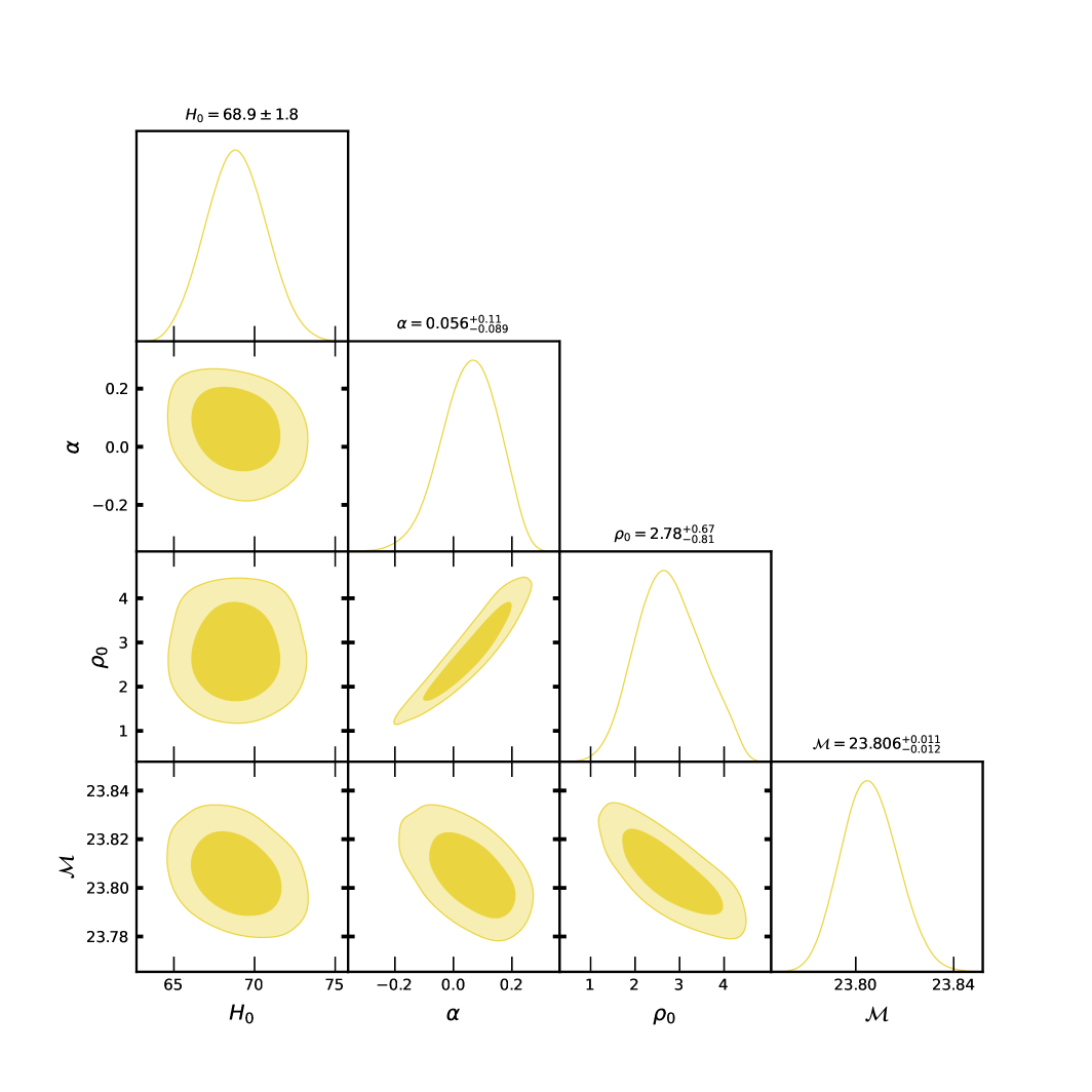
Figure 2: Model I: Marginalized $1\sigma$ and $2\sigma$ contour map with median values of $H_{0}$, $\alpha$ and $\rho_{0}$ using Joint data set.

5 Cosmic dynamics and the physical behavior

In this section, we investigate the dynamical characteristics of the universe evolution in model I and II by using the observationally constrained values of model parameters.

5.1 Cosmographic parameter

The study of cosmography was initially introduced by Weinberg [85], who used a Taylor series to introduced the scale factor that rose around present time $t_{0}$. A detailed overview of cosmography may be reviewed for different aspects of cosmographic parameters [23]. The Hubble parameter ($H$), has been considered as a variable observable quantity. The behavior of Hubble parameter (1) highlights that the expansion rate of the universe in considered models. The evolution of deceleration parameter $q$ is characterized through the second-order derivative of scale factor ($a$) [86]. To understand the universe’s cosmic evolution, the snap ($s$) and jerk ($j$) parameters serve as important tools. One of the cosmological parameter is the deceleration parameter that helps to characterize the universe’s expansion behavior. It is basically used to track down the rate of slowing down of the universe expansion. Mathematically, using the Hubble parameter and its derivative, it may be expressed as

$${}q=-1-\frac{\dot{H}}{H^{2}}.$$ (22)

This parameter serves as a tool to assess whether the universe is expanding at an increasing or decreasing rate. Depending on the value of $q$, different phases of cosmic expansion may be visualized. If $q$ is greater than zero $(q>0)$, the universe is in a decelerated phase. For $q<0$, the universe will expanding at an accelerating rate. For $-1<q<0$ the expansion follows a power-law acceleration. A super-exponential expansion era occurs in the universe for $q<-1$, while a de Sitter expansion when $q=-1$ [87, 88, 89, 90]. For matter and radiation-dominated universe expansion, the deceleration parameter will be $q=\frac{1}{2}$ and $q=1$ respectively. By using (15), (16) and (22), we may obtain for Model I and II as

$$q(z)=-1+\left({\frac{(1.5)(1+\alpha)(1+z)^{3+3\alpha}}{\rho_{0}+(1+z)^{3+3\alpha}}}\right)\ \ \text{and}$$ (23)

$$q(z)=-1+\frac{0.5(1+z)^{3}\left(3\Omega_{m0}+\left(\frac{3(1-\Omega_{m0})(1+z)^{3\alpha}(1+\alpha)}{(1+\rho_{0})}\right)\right)}{\left(\Omega_{m0}(1+z)^{3}+\frac{(1-\Omega_{m0})(\rho_{0}+(1+z)^{3+3\alpha})}{(1+\rho_{0})}\right)}$$ (24)

respectively.

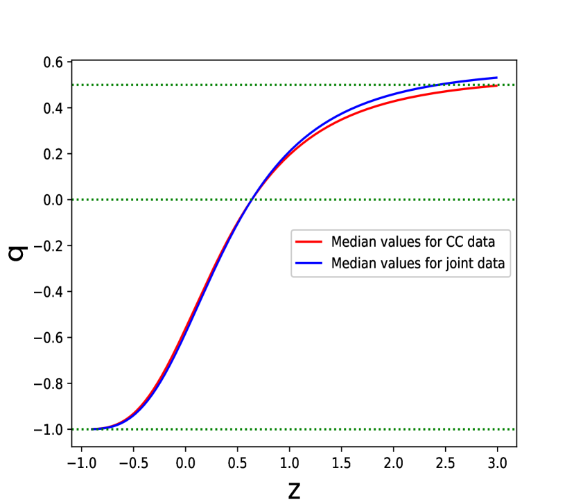
Figure 3: Model I: The deceleration parameter with $z$.

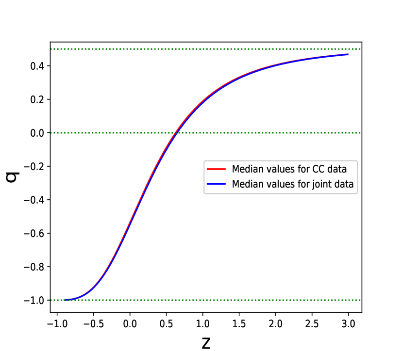
Figure 4: Model II: The deceleration parameter with $z$.

The behavior of $q(z)$ of model I (23) and model II (24) for the median values of parameters are illustrated in Fig. $(\ref{fig:7})$ and $(\ref{fig:8})$ respectively. Figures $(\ref{fig:7})$ and $(\ref{fig:8})$ indicate that in the early universe, $q(z)$ of these models is positive, while in the present times, it has becomes negative $q<0$ due to the domination of dark energy in models.

The deceleration parameter of these models provides insight into the universe’s transition from deceleration into acceleration of expansion. In model I, the present day value of deceleration parameter is $q=-0.56$ and $q=-0.58$ for CC and joint data respectively, and the value of transit red-shift are $z_{t}=0.638$ (for CC data) and $z_{t}=0.65$ (for joint data). The red-shift value at which $q=0$ is termed as the transit red-shift, since the behavior of $q$ is changing from positive to negative in the cosmic evolution. The accelerated universe expansion may be visualized in the model I for red-shifts $z<0.638$. For Model II, the transition from decelerated to accelerated expansion occur at $z_{t}=0.64$ based on CC estimates and at $z_{t}=0.647$ using joint estimates. For CC estimates, the deceleration parameter’s current value is $q_{0}=-0.536$, while for joint estimates, it is $q_{0}=-0.548$. These negative value of deceleration parameter of model I and II are confirming that the universe is expanding with acceleration in the present era $(z=0)$. And, thus it has been observed that the non-metricity scalar may yield the transiting universe evolution in model I governed by $f(Q)=C\sqrt{Q}$. In the Model II, the dark energy introduced by the non-metricity may yield the accelerated expansion at late-times while the cold dark matter yields the decelerated universe expansion at early times in model.

The behavior of $q$ in Fig. (4) and (4) suggests that these models will possess the matter-dominated era of universe expansion which may be confirmed with $(q\rightarrow\frac{1}{2})$ during early times. An accelerated phase $(q<0)$ in the present era and ultimately converges to the de Sitter scenario $(q=-1)$ as $z\rightarrow-1$. These models may explain the accelerated expansion universe at the present times, which is consistent with the observational data. It has been observed that the deceleration parameter of Model I and Model II are consistent with the current phase of accelerated expansion.
The jerk parameter $(j)$ indicates the rate at which the universe’s acceleration or deceleration changes over time. The snap parameter $(s)$ calculates the rate that the jerk parameter changes. These parameters are defined as follows:

$${}\mathit{j}=\frac{1}{aH^{3}}\left(\frac{d^{3}a}{dt^{3}}\right),\ \ \mathit{s}=\frac{1}{aH^{4}}\left(\frac{d^{4}a}{dt^{4}}\right)$$ (25)

In the present analysis, for $j$ and $s$, equation (25) can be rewritten in terms of red-shift [91].

$${}j(z)=q(z)\left(1+2q(z)\right)+\frac{dq}{dz}(1+z),\ \ \ \ s(z)=-\frac{dj}{dz}(1+z)-j(z)\left(2+3q(z)\right).$$ (26)

For Model I, based on the constrained values from the CC data set, the snap parameter is $s_{0}=-2.12$ and the jerk parameter $j_{0}=1.14$, however, from the joint estimates, the jerk parameter value is $j_{0}=1.25$ and snap parameter value is $s_{0}=-2.03$. Similarly, for Model II, the value of jerk parameter is $j_{0}=1.0164$ (for CC data set) and $j_{0}=1.017$ (for joint data set). In the Tables (1) and (2), we summarize the present day values of the cosmological parameters. For Models I and II, the value of jerk parameter exhibits a decreasing trend from early to late times, eventually approaching to $1$. This behavior suggests that these models differs from $\Lambda$CDM in the early universe but becomes similar to $\Lambda$CDM at later times.

5.2 The physical behavior of models based on the energy density, pressure and equation of state parameter

We highlight the physical behavior exhibited by the quantities such as the energy density and pressure. For the model parameters’s constrained values, the energy density has remained positive throughout the expansion history while the pressure may have undergone a recent transition to negative values. We calculate the energy density and pressure by utilizing equations (9), (15) and (16) as follows:

$$\rho_{d}(z)=3H_{0}^{2}\left[\frac{(1+z)^{3(1+\alpha)}+\rho_{0}}{\rho_{0}+1}\right]\quad\text{for Model I}{}$$ (27)

$$p_{d}(z)=\frac{3H_{0}^{2}(1+\alpha)(1+z)^{3+3\alpha}}{(\rho_{0}+1)}-3H_{0}^{2}\left[\frac{(1+z)^{3(1+\alpha)}+\rho_{0}}{\rho_{0}+1}\right]\quad\text{ for Model I}$$ (28)

$$\rho_{e}(z)=3H_{0}^{2}\left[\Omega_{m0}(1+z)^{3}+\left[\frac{1-\Omega_{m0}}{\rho_{0}+1}\right]\left[(1+z)^{3(1+\alpha)}+\rho_{0}\right]\right]\quad\quad\text{for Model II}$$ (29)

$$p_{e}(z)=3H_{0}^{2}(1+z)^{3}\left[\Omega_{m0}+\frac{(1-\Omega_{m0})(1+\alpha)(1+z)^{3\alpha}}{(1+\rho_{0})}\right]-3H_{0}^{2}\left[\Omega_{m0}(1+z)^{3}+\left[\frac{1-\Omega_{m0}}{\rho_{0}+1}\right]\left[(1+z)^{3(1+\alpha)}+\rho_{0}\right]\right]\quad\text{for Model II}$$ (30)

The evolution of energy density is depicted in figures (6) and figure (6) for Model I and II respectively. These figures are revealing that the energy densities in the models will be increasing with red-shift $(z)$ (decreases with cosmic time $(t)$), remaining positive throughout expansion for both the models. In other words, the energy densities will be decreasing from past to future. The energy densities will have positive values rules out the existence of finite-time future singularities in the models. During the early universe, at large red-shift ($z$), the pressure commences with positive values. In the later epoch along with the present epoch, the pressure becomes negative. It is observed from the graphical analysis that the non-metricity scalar will be responsible for the negative pressure necessary for the accelerated universe expansion in this late epoch.

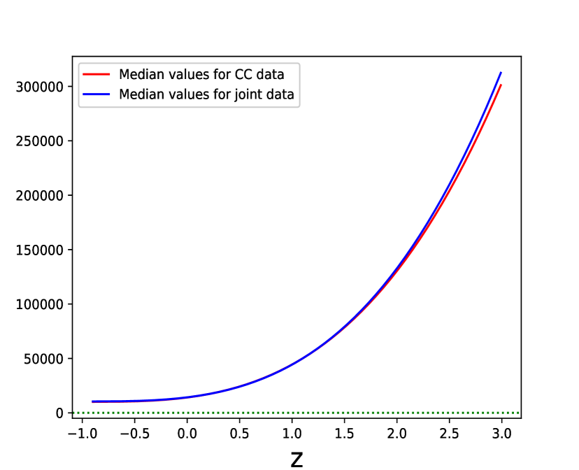
Figure 5: Model I: $\rho_{d}$ versus $\mathit{z}$

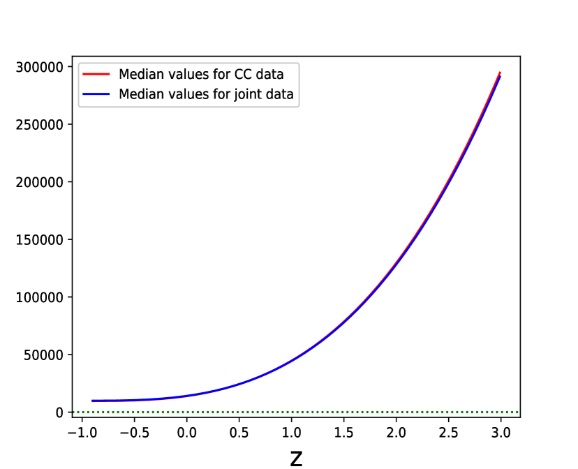
Figure 6: Model II: $\rho_{e}$ versus $\mathit{z}$

The EoS parameter may offer insights on the dominating fluid during the cosmic expansion of universe and thus helps to determine the dynamics of Universe. In the cosmological models, it may be commonly used to identify the nature of dark energy. The EoS parameter can be defined using the relationship between pressure $(p)$ and energy density $(\rho)$. It is mathematically expressed as $(\omega=\frac{p}{\rho})$. The cosmic characteristics, including the cold dark matter or dust dominated phase will have $\omega=0$ and, the radiation-dominated period will have $\omega=\frac{1}{3}$. The transition into an accelerated cosmic era happens for the equation of state parameter satisfying $\omega<-\frac{1}{3}$. The cosmic acceleration period may have three regimes: the quintessence-dominated regime for $-1<\omega<-\frac{1}{3}$, the cosmological constant-like state for $\omega=-1$ and phantom-dominated regime $\omega<-1$. In the Figs. (8) and (8), we provide the graphical representation of the EoS parameter evolution in the considered models.

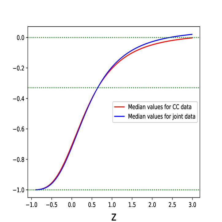
Figure 7: Model I: $\omega_{d}$ versus $z$

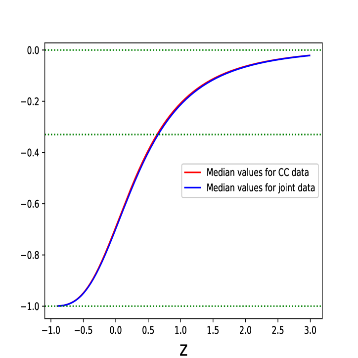
Figure 8: Model II: $\omega_{e}$ versus $z$

In the Model I, the EoS parameter values are estimated as $\omega_{d}=-0.706$ and $\omega_{d}=-0.720$ for CC and joint dataset respectively at $z=0$. Similarly, in the Model II, the effective EoS parameter values are obtained $\omega_{e}=-0.690$ (for CC dataset) and $\omega_{e}=-0.698$ (for joint dataset) at $z=0$. The Fig. (8) and (8) are revealing that the EoS parameter may correspond to the quintessence kind of dark energy in these models. At late-times, as $z\rightarrow-1$, the cosmological constant-like behavior may be visualized in these models. In the present era, the dark energy is a dynamical one which is varying with time in these models.

These models possess the past of matter-dominated expansion which are confirmed by Fig. (8) and (8) having $\omega=0$ during early times. The cosmic evolution is under the domination of quintessence kind of dark energy having $-1<\omega<-\frac{1}{3}$ in the present epoch, and ultimately converges towards the $\Lambda$CDM scenario $\omega=-1$ as $z\rightarrow-1$. For these evolution scenarios, we observe the role of non-metricity scalar having geometrical origin in the $f(Q)$ model. In the model I, the non-metricity is in charge for the matter dominated expansion and the dark energy dominated expansion. In this sense, the unified scenario has been confirmed in the affine EoS induced model of $f(Q)$ gravity. On the other hand, when the cold dark matter has been considered with the dark fluid satisfying affine EoS, the $f(Q)$ gravity model yields the lower $\Omega_{m0}$ value as compared to the $\Lambda$CDM model. The possible reasons for this change may be the matter-like characteristics possessed in the past by dark fluid having affine EoS. This is an important difference between the cosmic dynamics possessed by model without and with cold dark matter. In the model without dark matter, the fluid with affine EoS unifies the decelerated and accelerated expansion. While in the model with cold dark matter and fluid having affine EoS, the matter dominated era (having $q=\frac{1}{2}$) is controlled by both of these components leading to the $\omega_{e}=0$ scenario in effective sense.

5.3 Age of the Universe

The age of universe is an important criterion to test the viability of model as compared to the observable universe. The cosmic age $t(z)$ may be expressed in terms of the red-shift $z$ as  [92]

$${}t(z)=\int_{z}^{\infty}\frac{dz^{\prime}}{(1+z^{\prime})H(z^{\prime})}.$$ (31)

The present age$(t_{0})$ at $(z=0)$ has been calculated numerically using the integral consisting of the Hubble parameters $H(z)$ provided in equations (15) and (16).
In the Model I, the universe’s current age is $t_{0}$ (at $z=0)=13.51^{+0.08}_{-0.37}$ Gyr for CC data sets and $t_{0}=13.41^{+0.65}_{-1.04}$ Gyr for joint data sets, both of which are close with the current age values of the $\Lambda$CDM model (having $t_{0}=13.79$ Gyr) obtained from Planck results [5].
In model II, the universe present age value is $t_{0}=13.58^{+0.33}_{-0.22}$ Gyr and $t_{0}=13.59^{+0.69}_{-0.32}$ Gyr for CC and joint estimates respectively, both of which are again close with the current age values of the $\Lambda$CDM model mentioned above.

6 Conclusions

We probe the possibility to describe the unified scenario of universe expansion in $f(Q)$ gravity. The late-time accelerated expansion of the Universe has been investigated in $f(Q)$ gravity framework with affine equation of state (EoS) $(p_{d}=\alpha\rho_{d}-\rho_{0})$. In the $f(Q)$ model with affine EoS, we show that the unified scenario may be realized where the non-metricity may yield the transition from the decelerated expansion into accelerated expansion. In this model, a particular functional form $f(Q)=c\sqrt{Q}$ of $f(Q)$ gravity has been derived and it is shown that the matter dominated expansion may be also be explained with the non-metricity scalar in the model. On the other hand, we also study the model composed of cold dark matter and the dark fluid satisfying the affine EoS. A descriptive differences between these models have been studied.

We use the observational data of the CC and supernovae type Ia Pantheon data for the Markov Chain Monte Carlo (MCMC) analysis based on the Hubble parameters (15) and (16) of the derived models. A summary of the constrained values extracted from the MCMC application in the models are provided in Tables (1) and (2).

The evolution dynamics in the present study has been examined by study of the cosmological parameters. The behavior of deceleration parameter has been investigated. The evolution and dominant cosmic components during various epochs are reflected in the deceleration parameter behaviors of both models. The universe’s phase recently transitioned from decelerated to accelerated as indicated by the deceleration parameter’s evolution curve. In Model I, the estimated present deceleration parameter values are $q_{0}=-0.56$ and $q_{0}=-0.58$ for the CC and joint analyses respectively. For Model II, we obtain the deceleration parameter values at present as $q_{0}=-0.536$ and $q_{0}=-0.548$ based on the CC and joint data respectively. A negative deceleration parameter at $z=0$ demonstrates that cosmic expansion is accelerating for both models. At late-times, the negative pressure introduced by the non-metricity may be responsible for the accelerated universe expansion.
In the considered models, the physical behavior has been elaborated on the basis of energy density, pressure and EoS parameter for the model parameters’s constrained values . The energy density remains positive whereas pressure exhibits a change from positive to negative values. It is observed in the models that the cosmic accelerated expansion is caused by this negative pressure available in late era of the universe expansion. The behavior of energy density and pressure rules out the phantom evolution in the models. The varying dark energy evolution may correspond to the cosmological constant-like behavior in the asymptotic era having $z\rightarrow-1$.
In particular, for the model I, at $z=0$, $\omega_{d}=-0.706$ and $\omega_{d}=-0.720$ for CC and joint data respectively. These values at the present time suggest the existence of a quintessence-type dark energy in the model. Similarly, for the Model II, the EoS parameter values are obtained $\omega_{e}=-0.690$ (for CC dataset) and $\omega_{e}=-0.698$ (for joint dataset) at $z=0$. The graphical behavior reveals that the EoS parameter for dark energy exhibits quintessence kind of dark energy. In summary, the $f(Q)$ model with affine EoS is consistent with the observations of cosmic acceleration. The null energy condition’s validity in the models prohibits the model to possess finite-time future singularities.

For the $\Lambda$CDM model, the cosmological parameters are $q=-1$, $\omega=-1$, $j=1$, Snap $(s)=1$ during the asymptotic era as $z\rightarrow-1$. In the de-Sitter model of cosmic expansion, where $H$ remains constant and $q=-1$, $j=1$ and $s=1$. This indicates that the universe is undergoing exponential acceleration with the rate of change of both acceleration and jerk are increasing. In this context, for the Model I (Eq. 15), the dark energy equation of state (EoS) parameter ($\omega_{d})$ at present is near $-0.7$ and the deceleration parameter is approximately $-0.56$(for CC data) and $-0.58$(for joint data). In this scenario, the universe’s acceleration is attributed to dynamical dark energy and the jerk parameter is close to $\Lambda$CDM limit $(j=1)$ while the snap parameter is negative for the median values of model parameters. The Tables (1) and (2) highlight a summary of the results on cosmographic parameters. It is worthwhile to mentioned that these quantities will eventually align with the $\Lambda$CDM limits in the distant future. However, at present times, the cosmic dynamics of these model are differing from the $\Lambda$CDM model.

The age of universe is also estimated in the context of present $f(Q)$ gravity models. For model I, the value is $t_{0}=13.51^{+0.08}_{-0.37}$ Gyr and $t_{0}=13.41^{+0.65}_{-1.04}$ Gyr for CC and joint estimates respectively. For model II, the universe’s present age value is $t_{0}=13.58^{+0.33}_{-0.22}$ Gyr (for CC data) and $t_{0}=13.59^{+0.69}_{-0.32}$ Gyr (for joint data).

In summary, we show that the observationally compatible unified scenario may be realized in the $f(Q)$ gravity framework with the affine EoS. The non-metricity scalar may explain the matter dominated era of the past along with the dark energy dominated era of the observable universe. A descriptive difference between two class of models have illustrated that the present day matter density may have the lower value (as compared to $\Lambda$CDM model) in a model having cold dark matter and dark fluid satisfying affine EoS.

References

- [1] A. G. Riess, et al., Observational Evidence from Supernovae for an Accelerating Universe and a Cosmological Constant, Astronomical Journal 116 (3) (1998) 1009–1038. doi:https://doi.org/10.1086/300499.
- [2] S. Perlmutter, et al., Measurements of and from 42 High-Redshift Supernovae, Astrophysical Journal 517 (2) (1999) 565–586. doi:https://doi.org/10.1086/307221.
- [3] R. A. Knop, et al., New constraints on m, , and w from an independent set of 11 high-redshift supernovae observed with the hubble space telescope, The Astrophysical Journal 598 (1) (2003) 102. doi:https://doi.org/10.1086/378560.
- [4] J. L. Tonry, et al., Cosmological results from high-z supernovae, The Astrophysical Journal 594 (1) (2003) 1. doi:https://doi.org/10.1086/376865.
- [5] N. Aghanim, et al., Planck 2018 results. VI. Cosmological parameters, Astronomy and Astrophysics 641 (2020) A6. doi:https://doi.org/10.1051/0004-6361/201833910.
- [6] T. Padmanabhan, Cosmological constant—the weight of the vacuum, Physics reports 380 (5-6) (2003) 235–320. doi:https://doi.org/10.1016/S0370-1573(03)00120-0.
- [7] S. M. Carroll, The cosmological constant, Living reviews in relativity 4 (1) (2001) 1–56. doi:https://doi.org/10.12942/lrr-2001-1.
- [8] V. Sahni, A. Starobinsky, The case for a positive cosmological -term, International Journal of Modern Physics D 9 (04) (2000) 373–443. doi:https://doi.org/10.1142/S0218271800000542.
- [9] S. Tsujikawa, Modified gravity models of dark energy, in: Lectures on cosmology: Accelerated Expansion of the Universe, Springer, 2010, pp. 99–145. doi:https://doi.org/10.1007/978-3-642-10598-2_3.
- [10] S. Nojiri, S. D. Odintsov, Unified cosmic history in modified gravity: from f (r) theory to lorentz non-invariant models, Physics Reports 505 (2-4) (2011) 59–144. doi:https://doi.org/10.1016/j.physrep.2011.04.001.
- [11] S. Nojiri, S. D. Odintsov, V. K. Oikonomou, Modified gravity theories on a nutshell: Inflation, bounce and late-time evolution, Physics Reports 692 (2017) 1–104. doi:https://doi.org/10.1016/j.physrep.2017.06.001.
- [12] J. de Haro et al., Finite-time cosmological singularities and the possible fate of the universe, Physics Reports 1034 (2023) 1–114. doi:https://doi.org/10.1016/j.physrep.2023.09.003.
- [13] E. Di Valentino, et al., In the realm of the hubble tension—a review of solutions, Classical and Quantum Gravity 38 (15) (2021) 153001. doi:https://doi.org/10.1088/1361-6382/ac086d.
- [14] L. Heisenberg, Review on f (q) gravity, Physics Reports 1066 (2024) 1–78. doi:https://doi.org/10.1016/j.physrep.2024.02.001.
- [15] S. Weinberg, The cosmological constant problem, Reviews of modern physics 61 (1) (1989) 1. doi:https://doi.org/10.1103/RevModPhys.61.1.
- [16] H. A. Buchdahl, Non-linear lagrangians and cosmological theory, Monthly Notices of the Royal Astronomical Society 150 (1) (1970) 1–8. doi:https://doi.org/10.1093/mnras/150.1.1.
- [17] T. Harko, et al., f(r,t) gravity, Physical Review D—Particles, Fields, Gravitation, and Cosmology 84 (2) (2011) 024020. doi:https://doi.org/10.1103/PhysRevD.84.024020.
- [18] E. Elizalde, et al., cdm epoch reconstruction from f (r, g) and modified gauss–bonnet gravities, Classical and Quantum Gravity 27 (9) (2010) 095007. doi:https://doi.org/10.1088/0264-9381/27/9/095007.
- [19] K. Bamba, et al., Finite-time future singularities in modified gauss–bonnet and f(r, g) gravity and singularity avoidance, The European Physical Journal C 67 (2010) 295–310. doi:https://doi.org/10.1140/epjc/s10052-010-1292-8.
- [20] T. Harko, F. S. N. Lobo, f (, ) gravity, The European Physical Journal C 70 (2010) 373–379. doi:https://doi.org/10.1140/epjc/s10052-010-1467-3.
- [21] R. Chaubey, et al., The general class of bianchi cosmological models in f (r, t) gravity with dark energy in viscous cosmology, Indian Journal of Physics 90 (2016) 233–242. doi:https://doi.org/10.1007/s12648-015-0749-x.
- [22] Y. Xu, G. Li, T. Harko, S.-D. Liang, f(q, t) gravity, The European Physical Journal C 79 (2019) 708. doi:https://doi.org/10.1140/epjc/s10052-019-7207-4.
- [23] S. Capozziello, R. D’Agostino, O. Luongo, Extended gravity cosmography, International Journal of Modern Physics D 28 (10) (2019) 1930016. doi:https://doi.org/10.1142/S0218271819300167.
- [24] G. P. Singh, A. R. Lalke, N. Hulke, Study of particle creation with quadratic equation of state in higher derivative theory, Brazilian Journal of Physics 50 (2020) 725–743. doi:https://doi.org/10.1007/s13538-020-00788-1.
- [25] G. P. Singh, A. R. Lalke, Cosmological study with hyperbolic solution in modified f (q, t) gravity theory, Indian Journal of Physics 96 (14) (2022) 4361–4372. doi:https://doi.org/10.1007/s12648-022-02341-z.
- [26] R. Garg, et al., Cosmological model with linear equation of state parameter in f(r,lm) gravity, Phys. Lett. A 525 (2024) 129937. doi:10.1016/j.physleta.2024.129937.
- [27] S. Mandal, A. Singh, R. Chaubey, Cosmic evolution of holographic dark energy in f (q, t) gravity, International Journal of Geometric Methods in Modern Physics 20 (05) (2023) 2350084. doi:https://doi.org/10.1142/S0219887823500846.
- [28] A. R. Lalke, G. P. Singh, A. Singh, Late-time acceleration from ekpyrotic bounce in f (q, t) gravity, International Journal of Geometric Methods in Modern Physics 20 (08) (2023) 2350131. doi:https://doi.org/10.1142/S0219887823501311.
- [29] A. Singh, Lyra cosmologies with the dynamical system perspective, Physica Scripta 99 (4) (2024) 045011. doi:https://doi.org/10.1088/1402-4896/ad302a.
- [30] S. Capozziello, V. De Falco, C. Ferrara, The role of the boundary term in f (q, b) symmetric teleparallel gravity, The European Physical Journal C 83 (10) (2023) 915. doi:https://doi.org/10.1140/epjc/s10052-023-12072-y.
- [31] G. P. Singh, R. Garg, A. Singh, A generalized lambda cdm model with parameterized hubble parameter in particle creation, viscous and model framework, International Journal of Geometric Methods in Modern Physics (2024). doi:https://doi.org/10.1142/S0219887825501117.
- [32] A. Singh, Dynamical systems of modified gauss–bonnet gravity: cosmological implications, The European Physical Journal C 85 (2025) 24. doi:https://doi.org/10.1140/epjc/s10052-024-13732-3.
- [33] J. B. Jiménez, L. Heisenberg, T. Koivisto, Coincident general relativity, Physical Review D 98 (4) (2018) 044048. doi:https://doi.org/10.1103/PhysRevD.98.044048.
- [34] W. Yang, et al., 2021-h0 odyssey: closed, phantom and interacting dark energy cosmologies, Journal of Cosmology and Astroparticle Physics 2021 (10) (2021) 008. doi:https://doi.org/10.1088/1475-7516/2021/10/008.
- [35] R. Lazkoz, et al., Observational constraints of f (q) gravity, Physical Review D 100 (10) (2019) 104027. doi:https://doi.org/10.1103/PhysRevD.100.104027.
- [36] F. Esposito, et al., Reconstructing isotropic and anisotropic f (q) cosmologies, Physical Review D 105 (8) (2022) 084061. doi:https://doi.org/10.1103/PhysRevD.105.084061.
- [37] T. Harko, et al., Coupling matter in modified q gravity, Physical Review D 98 (8) (2018) 084043. doi:https://doi.org/10.1103/PhysRevD.98.084043.
- [38] D. C. Maurya, A. Dixit, A. Pradhan, Transit string dark energy models in f (q) gravity, International Journal of Geometric Methods in Modern Physics 20 (08) (2023) 2350134. doi:https://doi.org/10.1142/S0219887823501347.
- [39] A. Pradhan, A. Dixit, D. C. Maurya, Quintessence behavior of an anisotropic bulk viscous cosmological model in modified f(q)-gravity, Symmetry 14 (12) (2022) 2630. doi:https://doi.org/10.3390/sym14122630.
- [40] S. Capozziello, et al., Preserving quantum information in f (q) non-metric gravity cosmology, The European Physical Journal C 84 (10) (2024) 1081. doi:https://doi.org/10.1140/epjc/s10052-024-13449-3.
- [41] S. Nojiri, S. D. Odintsov, Well-defined f (q) gravity, reconstruction of flrw spacetime and unification of inflation with dark energy epoch, Physics of the Dark Universe (2024) 101538doi:https://doi.org/10.1016/j.dark.2024.101538.
- [42] K. Hu, et al., Nonpropagating ghost in covariant f(q) gravity, Physical Review D 108 (12) (2023) 124030. doi:https://doi.org/10.1103/PhysRevD.108.124030.
- [43] S. Capozziello, R. D’Agostino, Model-independent reconstruction of f (q) non-metric gravity, Physics Letters B 832 (2022) 137229. doi:https://doi.org/10.1016/j.physletb.2022.137229.
- [44] N. Dimakis, A. Paliathanasis, M. Roumeliotis, T. Christodoulakis, Flrw solutions in f (q) theory: The effect of using different connections, Physical Review D 106 (4) (2022) 043509. doi:https://doi.org/10.1103/PhysRevD.106.043509.
- [45] A. Paliathanasis, Dipole cosmology in fq-gravity, Physics of the Dark Universe 46 (2024) 101585. doi:https://doi.org/10.1016/j.dark.2024.101585.
- [46] L. Heisenberg, M. Hohmann, S. Kuhn, Cosmological teleparallel perturbations, Journal of Cosmology and Astroparticle Physics 2024 (03) (2024) 063. doi:https://doi.org/10.1088/1475-7516/2024/03/063.
- [47] S. Capozziello, V. De Falco, C. Ferrara, Comparing equivalent gravities: common features and differences, The European Physical Journal C 82 (10) (2022) 865. doi:https://doi.org/10.1140/epjc/s10052-022-10823-x.
- [48] R. Garg, G. P. Singh, A. Singh, Observational constraints on gong-zhang parametrizations in gravity, arXiv preprint arXiv:2410.18568 (2024).
- [49] M. Koussour, et al., Square-root parametrization of dark energy in f(q) cosmology, Communications in Theoretical Physics 75 (12) (2023) 125403. doi:https://doi.org/10.1088/1572-9494/ad0830.
- [50] S. Rani, et al., Physical viability of f(q) gravity corrected charged anisotropic solutions, Physics of the Dark Universe 47 (2025) 101754. doi:https://doi.org/10.1016/j.dark.2024.101754.
- [51] P. Sarmah, U. D. Goswami, Dynamical system analysis of lrs-bi universe with f(q) gravity theory, Physics of the Dark Universe 46 (2024) 101556. doi:https://doi.org/10.1016/j.dark.2024.101556.
- [52] S. K. Maurya, et al., Self-bound isotropic models in f(q) gravity and effect of f(q) parameter on mass–radius relation and stability of compact objects, Physics of the Dark Universe 46 (2024) 101619. doi:https://doi.org/10.1016/j.dark.2024.101619.
- [53] G. G. L. Nashed, S. Nojiri, General geometry realized by four-scalar model and application to f(q) gravity, Physics of the Dark Universe 46 (2024) 101655. doi:https://doi.org/10.1016/j.dark.2024.101655.
- [54] S. Capozziello, M. Capriolo, Gravitational waves in f(q) non-metric gravity without gauge fixing, Physics of the Dark Universe 45 (2024) 101548. doi:https://doi.org/10.1016/j.dark.2024.101548.
- [55] F. Parsaei, S. Rastgoo, P. K. Sahoo, Wormhole in f(q) gravity, The European Physical Journal Plus 137 (9) (2022) 1–16. doi:https://doi.org/10.1140/epjp/s13360-022-03298-y.
- [56] E. Babichev, V. Dokuchaev, Y. Eroshenko, Dark energy cosmology with generalized linear equation of state, Class. Quantum Grav. 22 (2005) 143. doi:https://doi.org/10.1088/0264-9381/22/1/010.
- [57] T. Chiba, N. Sugiyama, T. Nakamura, Cosmology with x-matter, Mon. Not. R. Astron. Soc. 289 (1997) L5–L9. doi:https://doi.org/10.1093/mnras/289.2.L5.
- [58] E. Babichev, V. Dokuchaev, Y. Eroshenko, Black hole mass decreasing due to phantom energy accretion, Phys. Rev. Lett. 93 (2004) 021102. doi:https://doi.org/10.1103/PhysRevLett.93.021102.
- [59] H. Stefancic, Expansion around the vacuum equation of state: Sudden future singularities and asymptotic behavior, Phys. Rev. D 71 (2005) 084024. doi:https://doi.org/10.1103/PhysRevD.71.084024.
- [60] K. Ananda, M. Bruni, Cosmological dynamics and dark energy with a nonlinear equation of state: A quadratic model, Phys. Rev. D 74 (2006) 023523. doi:https://doi.org/10.1103/PhysRevD.74.023523.
- [61] A. Balbi, M. Bruni, C. Quercellini, dm: Observational constraints on unified dark matter with constant speed of sound, Phys. Rev. D 76 (2007) 103519. doi:https://doi.org/10.1103/PhysRevD.76.103519.
- [62] T. Singh, R. Chaubey, Bianchi type-i universe with wet dark fluid, Pramana - J. Phys. 71 (2008) 447–458. doi:https://doi.org/10.1007/s12043-008-0124-y.
- [63] R. Chaubey, Bianchi type-v universe with wet dark fluid, Astrophys. Space Sci. 321 (2009) 241–246. doi:https://doi.org/10.1007/s10509-009-0027-5.
- [64] G. Khadekar, Brane kantowski-sachs universe with linear equation of state and a future singularity, Gravit. Cosmol. 21 (2015) 334–339. doi:https://doi.org/10.1134/S020228931504009X.
- [65] G. P. Singh, N. Hulke, A. Singh, Thermodynamical and observational aspects of cosmological model with linear equation of state, Int. J. Geom. Methods Mod. Phys. 15 (2018) 1850129. doi:https://doi.org/10.1142/S0219887818501293.
- [66] A. Singh, K. C. Mishra, Aspects of some rastall cosmologies, Eur. Phys. J. Plus 135 (2020) 752. doi:https://doi.org/10.1140/epjp/s13360-020-00783-0.
- [67] A. Singh, R. Raushan, R. Chaubey, Qualitative aspects of rastall gravity with barotropic fluid, Can. J. Phys. 99 (2021) 1073–1081. doi:https://doi.org/10.1139/cjp-2020-0061.
- [68] A. Singh, G. P. Singh, A. Pradhan, Cosmic dynamics and qualitative study of rastall model with spatial curvature, Int. J. Mod. Phys. A 37 (2022) 2250104. doi:https://doi.org/10.1142/S0217751X22501044.
- [69] A. Singh, Homogeneous and anisotropic cosmologies with affine eos: a dynamical system perspective, The European Physical Journal C 83 (2023) 696. doi:https://doi.org/10.1140/epjc/s10052-023-11879-z.
- [70] G. Mustafa, F. Javed, S. K. Maurya, S. Ray, Possibility of stable thin-shell around wormholes within string cloud and quintessential field via the van der waals and polytropic eos, Chinese J. Phys. 88 (2024) 32–54. doi:https://doi.org/10.1016/j.cjph.2023.12.035.
- [71] A. Singh, S. Krishnannair, Affine eos cosmologies: observational and dynamical system constraints, Astronomy and Computing 47 (2024) 100827. doi:https://doi.org/10.1016/j.ascom.2024.100827.
- [72] J. B. Jiménez, et al., Cosmology in f(q) geometry, Physical Review D 101 (10) (2020) 103507. doi:https://doi.org/10.1103/PhysRevD.101.103507.
- [73] P. J. E. Peebles, B. Ratra, The cosmological constant and dark energy, Rev. Mod. Phys. 75 (2003) 559–606. doi:https://doi.org/10.1103/RevModPhys.75.559.
- [74] G. F. R. Ellis, R. Maartens, M. A. H. MacCallum, Causality and the speed of sound, Gen. Relativ. Gravit 39 (2007) 1651–1660. doi:https://doi.org/10.1007/s10714-007-0479-2.
- [75] D. Foreman-Mackey et al., emcee: the mcmc hammer, Publications of the Astronomical Society of the Pacific 125 (925) (2013) 306. doi:10.1086/670067.
- [76] S. Vagnozzi, A. Loeb, M. Moresco, Eppur è piatto? the cosmic chronometers take on spatial curvature and cosmic concordance, The Astrophysical Journal 908 (1) (2021) 84. doi:https://doi.org/10.3847/1538-4357/abd4df.
- [77] G. S. Sharov, V. O. Vasiliev, How predictions of cosmological models depend on hubble parameter data sets, arXiv preprint arXiv:1807.07323 (2018). doi:https://doi.org/10.26456/mmg/2018-611.
- [78] R. Jimenez, A. Loeb, Constraining cosmological parameters based on relative galaxy ages, The Astrophysical Journal 573 (1) (2002) 37. doi:https://doi.org/10.1086/340549.
- [79] A. R. Lalke, G. P. Singh, A. Singh, Cosmic dynamics with late-time constraints on the parametric deceleration parameter model, The European Physical Journal Plus 139 (3) (2024) 288. doi:https://doi.org/10.1140/epjp/s13360-024-05091-5.
- [80] S. Mandal, A. Singh, R. Chaubey, Late-time constraints on barotropic fluid cosmology, Physics Letters A 519 (2024) 129714. doi:https://doi.org/10.1016/j.physleta.2024.129714.
- [81] A. Singh, S. Mandal, R. Chaubey, R. Raushan, Observational constraints on the expansion scalar and shear relation in the locally rotationally symmetric bianchi i model, Phys. Dark Uni. 47 (2025) 101798. doi:https://doi.org/10.1016/j.dark.2024.101798.
- [82] D. M. Scolnic, et al., The complete light-curve sample of spectroscopically confirmed sne ia from pan-starrs1 and cosmological constraints from the combined pantheon sample, The Astrophysical Journal 859 (2) (2018) 101. doi:https://doi.org/10.3847/1538-4357/aab9bb.
- [83] G. F. R. Ellis, R. Maartens, M. A. MacCallum, Relativistic cosmology, Cambridge University Press, 2012. doi:http://dx.doi.org/10.1017/CBO9781139014403.
- [84] K. Asvesta, et al., Observational constraints on the deceleration parameter in a tilted universe, Monthly Notices of the Royal Astronomical Society 513 (2) (2022) 2394–2406. doi:https://doi.org/10.1093/mnras/stac922.
- [85] S. Weinberg, Cosmology oxford university press (2008).
- [86] A. Mukherjee, N. Banerjee, Parametric reconstruction of the cosmological jerk from diverse observational data sets, Physical Review D 93 (4) (2016) 043002. doi:https://doi.org/10.1103/PhysRevD.93.043002.
- [87] A. Singh, Qualitative study of anisotropic cosmologies with inhomogeneous equation of state, Chinese Journal of Physics 88 (2024) 865–878. doi:https://doi.org/10.1016/j.cjph.2024.02.011.
- [88] A. Singh, et al., Lagrangian formulation and implications of barotropic fluid cosmologies, International Journal of Geometric Methods in Modern Physics 19 (07) (2022) 2250107. doi:https://doi.org/10.1142/S0219887822501079.
- [89] A. Singh, S. Krishnannair, Varying vacuum models with spatial curvature: a dynamical system perspective, Gen. Relativ. Gravit 56 (2024) 31. doi:https://doi.org/10.1007/s10714-024-03219-7.
- [90] A. Singh, Role of dynamical vacuum energy in the closed universe: implications for bouncing scenario, Gen. Relativ. Gravit 56 (2024) 138. doi:https://doi.org/10.1007/s10714-024-03325-6.
- [91] F. Y. Wang, Z. G. Dai, S. Qi, Probing the cosmographic parameters to distinguish between dark energy and modified gravity models, Astronomy & Astrophysics 507 (1) (2009) 53–59. doi:https://doi.org/10.1051/0004-6361/200911998.
- [92] M.-L. Tong, Y. Zhang, Cosmic age, statefinder, and om diagnostics in the decaying vacuum cosmology, Physical Review D 80 (2) (2009) 023503. doi:https://doi.org/10.1103/PhysRevD.80.023503.