An Analytical Theory of Power Law Spectral Bias
in the Learning Dynamics of Diffusion Models

Binxu Wang
Abstract

We developed an analytical framework for understanding how the learned distribution evolves during diffusion model training. Leveraging the Gaussian equivalence principle, we derived exact solutions for the gradient-flow dynamics of weights in one or two layer linear denoiser settings with arbitrary data. Remarkably, these solutions allowed us to derive the generated distribution in closed-form and its KL-divergence through training. These analytical results exposes a pronounced power law spectral bias, i.e. for weights and distributions, convergence time of a mode follows a inverse power law of its variance. Empirical experiments on both Gaussian and image datasets demonstrate that the power-law spectral bias—remain robust even when using deeper or convolutional architectures. Our results underscore the importance of the data covariance in dictating the order and rate at which diffusion models learn different modes of the data, providing potential explanations of why earlier stopping could lead to incorrect details in image generative model.

Diffusion Models, Learning Dynamics, Analytical Theory, Spectral Bias, Power Law

Refer to caption

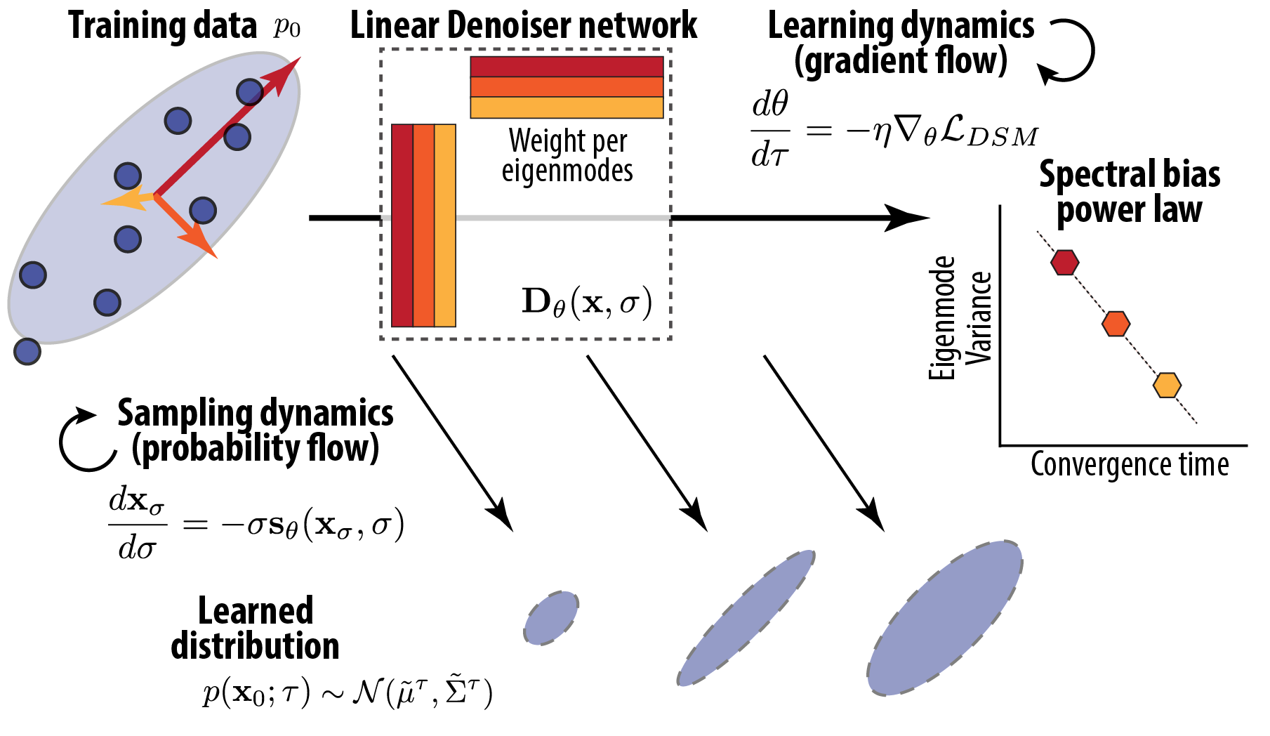
Figure 1: Graphical summary. The interaction of learning and sampling dynamics leads to a power-law spectral bias in the generated distribution along eigenmodes.

1 Introduction

Diffusion models have emerged as a leading approach in generative modeling, achieving remarkable success in domains ranging from image and video to molecular design (Sohl-Dickstein et al., 2015; Song & Ermon, 2019b; Dhariwal & Nichol, 2021; Ho et al., 2020). At their core, diffusion models learn a series of denoisers or score functions that invert a progressive noising process applied to data. By integrating the learned score with the probability flow ordinary differential equation (ODE), one can transform noise to samples from target distribution.

Despite the rapid progress in diffusion models, several fundamental questions about their training dynamics and convergence behavior remain unanswered. In particular, how does the learned distribution evolve during training and how does early stopping affects it? Moreover, empirical observations suggest that certain intricate details—especially those tied to less dominant modes in the data distribution—tend to be not accurately captured. For instance, generated human image often display unnatural fingers or awkward eye features, suggesting potential training or capacity limitations for lower-variance modes in the data.

Main Contribution. To gain analytical insights, we focus on a linear denoiser setting (e.g. a deep linear network). In this setting, we found arbitrary training distribution is equivalent to the Gaussian with matched mean and covariance. This allows us to derive closed form solutions to the learning dynamics of weights and the generated distribution, in a few settings. These solutions exposed the spectral bias in distribution learning: eigenmodes with larger variances converge rapidly, while those with smaller variances converge slowly, following an inverse power law (Fig. 1). This spectral bias was validated in practical diffusion training settings with deep nonlinear networks. This bias could explain the artifacts that arise when training is truncated early: high-variance modes dominate, leaving low-variance modes undertrained and producing inaccuracies in fine-grained details. All proofs and extended derivations are deferred to the appendices.

2 Related Work and Motivation: Spectral Bias in Distribution Learning

Spectral Structure in Natural Data

Many natural data distributions have interesting spectral structures (e.g. image (Torralba & Oliva, 2003), sound (Attias & Schreiner, 1996), video (Dong & Atick, 1995)): the data covariance eigenvalues follow power law, and eigenvectors have interesting meanings (e.g. face (Turk & Pentland, 1991; Wang & Ponce, 2021)). These structures interact with the learning dynamics of machine learning models in an interesting way. Understanding such structure and learning could potentially predict the order of learning certain features in large scale models. Leveraging such structure may inform us how to pre-condition the data or build in inductive bias to help the machine learning methods learn more efficiently.

Hidden Gaussian Structure in Diffusion Model

Recently, a line of work found, the learned neural score can be well approximated by the linear score of the Gaussian approximation of the data for most of the signal to noise ratios (Wang & Vastola, 2023). Substituting neural score with such linear score can accelerate sampling speed or improve sampling quality (Wang & Vastola, 2024). People also found this structure associated with the generalization-memorization transition of diffusion models (Li et al., 2024). In summary, the existence of this structure shows, the learned score approximator is dominated by the linear score of Gaussian approximation of data at many noise levels. Thus, it’s reasonable to hypothesize this Gaussian structure will have significant effect on the learning dynamics of score approximator. This inspired us to consider first the linear score approximator which can only learn the Gaussian structure (mean and covariance) in data.

Learning Theory of (Ridge) Regression

Regression problem and its gradient learning dynamics have been thoroughly examined by numerous theoretical works (Rahaman et al., 2019; Bordelon et al., 2020; Canatar et al., 2021). Diffusion models are also trained by solving a regression problem, i.e. predicting the flow vector field from the noised data points with quadratic loss. From this perspective, many classic results apply to the analysis of diffusion models. However, there are a few key difference that set diffusion apart from the classic analysis of regression problems: 1) in the denoising score matching (DSM) loss, there is noise in both predictor and predicting target; 2) diffusion model has a sampling process, thus the interesting quantity to us is not simply the error in score prediction, but the generated distribution and its divergence from the “ground truth” one. These additional complexity, especially the interaction of learning and sampling dynamics, makes the theoretical analysis of the “spectral bias” in diffusion models challenging. Our paper’s primary contribution is the development of a solvable model to understand this interaction, which we then leverage to derive insights for practical applications.

3 Foundation: Learning in Diffusion Models with Linear Denoiser

3.1 Score-based Diffusion Models

We will follow the convention and notations in (Karras et al., 2022) throughout this paper. Consider a data distribution $p(\mathbf{x}_{0})$ to model, the score function $\nabla\log p(\mathbf{x},\sigma)$ is the gradient of the log data density convolved by Gaussian $\mathcal{N}(0,\sigma^{2}I)$. Diffusion model leverages the probability flow Ordinary Differential Equation (ODE),

$\displaystyle d\mathbf{x}=-\sigma\nabla_{\mathbf{x}}\log p(\mathbf{x},\sigma)d\sigma$ (1)

When evolving a sample $\mathbf{x}_{\sigma_{T}}\sim p(\mathbf{x},\sigma_{T})$ along the PF-ODE to $\sigma_{0}$, the solution $\mathbf{x}_{\sigma_{0}}$ will suffice $\mathbf{x}_{\sigma_{0}}\sim p(\mathbf{x},\sigma_{0})$, i.e. reversing the noising process if $\sigma_{T}>\sigma_{0}$. To learn the score of a data distribution $p_{0}(\mathbf{x})$, we can minimize the denoising score matching (DSM) objective (Vincent, 2011) with a function approximator. We reparametrize the score with the optimal ‘denoiser’ $\mathbf{s}_{\theta}(\mathbf{x},\sigma)=(\mathbf{D}_{\theta}(\mathbf{x},\sigma)-\mathbf{x})/\sigma^{2}$ The DSM objective at noise level $\sigma$ reads

$\displaystyle\mathcal{L}_{\sigma}\;=\;\mathbb{E}_{\mathbf{x}_{0}\sim p_{0},\;\mathbf{z}\sim\mathcal{N}(0,I)}\Bigl{\|}\mathbf{D}_{\theta}(\mathbf{x}_{0}+\sigma\mathbf{z};\sigma)\;-\;\mathbf{x}_{0}\Bigr{\|}_{2}^{2}.$ (2)

Weighting functions in DSM objective To balance the loss and importance from different noise scales, practical diffusion models all adopted certain weighting functions in their overall loss $\mathcal{L}=\int_{\sigma}d\sigma\,\,w(\sigma)\,\mathcal{L}_{\sigma}$

3.2 Gaussian Data and Optimal Denoiser

To motivate our linear score approximator set up, it’s useful to consider the score and denoiser of a Gaussian distribution, which are linear functions. For Gaussian data $\mathbf{x}_{0}\sim\mathcal{N}(\bm{\mu},\bm{\Sigma}),\mathbf{x}_{0}\in\mathbb{R}^{d}$ where $\bm{\Sigma}$ is positive semi-definite. When noising $\mathbf{x}_{0}$ by $\sigma$-scaled Gaussian noise, the corrupted $\mathbf{x}$ satisfies $\mathbf{x}\,\sim\,\mathcal{N}(\bm{\mu},\,\bm{\Sigma}+\sigma^{2}\mathbf{I})$. The optimal denoiser and corresponding score function are known to be

$\displaystyle\mathbf{D}^{*}(\mathbf{x};\sigma)\;=$ $\displaystyle\;\bm{\mu}+(\bm{\Sigma}+\sigma^{2}\mathbf{I})^{-1}\bm{\Sigma}(\mathbf{x}-\bm{\mu}),$ (3)
$\displaystyle\mathbf{s}^{*}(\mathbf{x};\sigma)\;=$ $\displaystyle\;\nabla_{\mathbf{x}}\log p(\mathbf{x},\sigma)=\frac{1}{\sigma^{2}}\bigl{[}\mathbf{D}^{*}(\mathbf{x};\sigma)-\mathbf{x}\bigr{]}.$ (4)

Minimizing (2) for Gaussian data yields $\mathbf{D}^{*}$.

Remark 3.1.

This solution has an intuitive interpretation, i.e. the difference of state and distribution mean was projected onto the eigenbasis and shrinked mode-by-mode by $\frac{\lambda_{k}}{\lambda_{k}+\sigma^{2}}$. Thus, according to the variance $\lambda_{k}$ along target axis, modes with variance significantly higher than noise $\lambda_{k}\gg\sigma^{2}$ will be retained; modes with variance much smaller than noise will be “shrinked” out. Effectively $\sigma^{2}$ defined a threshold of signal and noise, and modes below which will be removed.

3.3 Gradient Flow Dynamics of Linear Denoiser

We start by considering a linear function as the denoiser for a given noise level $\sigma$. The simplest parametrization will be the following one,

$\displaystyle\mathbf{D}(\mathbf{x};\sigma)\;=\;\mathbf{W}\,\mathbf{x}\;+\;\mathbf{b}.$ (5)

The commonly used residual connection from $\mathbf{x}$ can be regarded as an alternative parametrization $\mathbf{W}=c_{skip}I+c_{out}\mathbf{W}^{\prime}$ (Karras et al., 2022). Later we will consider deeper linear networks, such as the symmetric two-layer network $PP^{\intercal}\mathbf{x}+\mathbf{b}$, which can also be regarded as alternative parametrization of the weight $\mathbf{W}$.

Gaussian equivalence

We consider “full-batch” training on (2), i.e. taking the full expectation over $\mathbf{x}_{0}\sim p_{0},\mathbf{z}\sim\mathcal{N}(0,I)$ 111This is somewhat less practical than the full batch learning in normal supervised learning. For diffusion, even with finite number of training samples $\{\mathbf{x}_{0}\}$ it’s infeasible to sample all noise $\mathbf{z}$ in a batch. . Here, training distribution $p_{0}$ is an arbitrary distribution with finite mean and covariance, $\mu$ and $\bm{\Sigma}$. We exploit the fact of Gaussian equivalence when score approximator is linear: in terms of loss, the data is equivalent to the Gaussian distribution with matching first two moments. To see it, the full batch loss is a quadratic form of $\mathbf{W}$ and $\mathbf{b}$, which only depends on the mean and covariance of $\mathbf{x}$. (derivation in Sec. B.1)

$\displaystyle\mathcal{L}_{\sigma}=\|b-(I-W)\mu\|_{2}^{2}+\mbox{Tr}[W^{\intercal}W(\sigma^{2}I+\Sigma)]$
$\displaystyle-2\mbox{Tr}[W^{\intercal}\Sigma]+\mbox{Tr}[\Sigma]$ (6)

Let $\bm{\Sigma}=\sum_{k}\lambda_{k}\mathbf{u}_{k}\mathbf{u}_{k}^{\intercal}$ be the eigen-decomposition of the covariance matrix, with the eigenvectors $[\mathbf{u}_{1},..\mathbf{u}_{d}]$ forming an orthonormal basis, and $\lambda_{1},...\lambda_{d}$ the associated variance along each principal component. This eigenbasis will be critical to the analysis below.

Gradient

Differentiating this quadratic loss yields gradients that depend linearly on the parameters,

$\displaystyle\nabla_{b}\mathcal{L}_{\sigma}$ $\displaystyle=2(b-(I-\mathbf{W})\bm{\mu})$ (7)
$\displaystyle\nabla_{\mathbf{W}}\mathcal{L}_{\sigma}$ $\displaystyle=-2\bm{\Sigma}+2\mathbf{W}(\sigma^{2}\mathbf{I}+\bm{\Sigma})+\nabla_{b}\mathcal{L}_{\sigma}\mu^{\intercal}$ (8)
Global optimum

Setting the gradients to zero yields the unique global optimum, which recovers the optimal Gaussian denoiser (Eq.3):

$\displaystyle\mathbf{W}^{*}\;=\;\bm{\Sigma}\,(\bm{\Sigma}+\sigma^{2}\mathbf{I})^{-1},\quad\mathbf{b}^{*}\;=\;(\mathbf{I}-\mathbf{W}^{*})\,\bm{\mu}.$ (9)

With this optimal solution, we can see the minimum of DSM loss across all linear denoisers is

$\displaystyle\min_{\mathbf{W},b}\mathcal{L}_{\sigma}=\sigma^{2}\mbox{Tr}[\Sigma(\sigma^{2}I+\Sigma)^{-1}]$ (10)

and cannot be optimized to zero.

Training dynamics

This work will majorly consider the gradient flow dynamics, denoting training time $\tau$ with learning rate $\eta$. Results for discrete gradient descent are showed in Sec. C.1.1.

$\displaystyle\frac{d\mathbf{W}}{d\tau}=-\eta\nabla_{\mathbf{W}}\mathcal{L_{\sigma}}\;,\;\frac{d\mathbf{b}}{d\tau}=-\eta\nabla_{\mathbf{b}}\mathcal{L_{\sigma}}$ (11)

In this paper, we will consider a few set ups that we can gain analytical insights on the gradient flow dynamics, which could be leveraged to analyze the generated distribution.

3.4 Sampling Dynamics with Learned Linear Score

For diffusion models, our main focus is on the generated distribution rather than the predicted score. To obtain this distribution, we solve the probability flow ODE or SDE by integrating the learned score across the noise scales $\sigma$, from from $\sigma_{T}$ down to $\sigma_{min}\approx 0$. For linear denoisers, PF-ODE reads

$\displaystyle\frac{d}{d\sigma}\mathbf{x}=-\sigma\frac{\mathbf{D}(\mathbf{x},\sigma)-\mathbf{x}}{\sigma^{2}}=-\bigl{(}\frac{\mathbf{W}(\sigma)-\mathbf{I}}{\sigma}\mathbf{x}+\frac{\mathbf{b}(\sigma)}{\sigma}\bigr{)}$ (12)

where $\mathbf{W}(\sigma)$ and $\mathbf{b}(\sigma)$ are the linear parameter for each noise scale $\sigma$. For the purpose of analytical tractability, we assume weights at different noise scales $\mathbf{W}(\sigma)$ are independent from each other, and it’s trained only on the loss at given noise scale $\mathcal{L}_{\sigma}$, potentially weighted by a factor. This is effectively assuming the model had a separate weight matrix $\mathbf{W}(\sigma)$ at each $\sigma$ level, which is obviously idealistic and not how practically diffusion models are parametrized. Later, we’ll demonstrate that this assumption can be relaxed based on our empirical findings.

Remark 3.2.

Eq.(12) is a linear inhomogeneous ODE with time varying dynamic matrix, thus its solution $\mathbf{x}_{\sigma}$ is a linear function of the initial condition $\mathbf{x}_{T}$ (Hartman, 2002). Since the initial noise $\mathbf{x}_{T}\sim\mathcal{N}(0,\sigma^{2}_{T}I)$, at any noise scale $\sigma$, $\mathbf{x}_{\sigma}$ is also Gaussian distributed, with mean and covariance determined by the linear function. Generally, if the weight matrices do not commute, this ODE cannot be solved in closed form. However, when the weight matrices $W(\sigma)$ at different noise levels share the same eigenbasis, i.e. commute, it could be integrated mode-by-mode. This is exactly the case, when the denoiser is the Gaussian linear one (Eq.3), then Eq.12 admits a closed form solution to the sampling trajectory (Pierret & Galerne, 2024; Wang & Vastola, 2023).

Proposition 3.3.

Assuming weights at each $\sigma$ share the eigenbasis $\mathbf{u}_{k}$, $\mathbf{W}_{\sigma}=\sum_{k}\psi_{k}(\sigma)\mathbf{u}_{k}\mathbf{u}_{k}^{\intercal}$, $\mathbf{b}_{\sigma}=\sum_{k}b_{k}(\sigma)\mathbf{u}_{k}$, and the solution $\mathbf{x}(\sigma)=\sum_{k}c_{k}(\sigma)\mathbf{u}_{k}$. Then representing the PF-ODE on eigenbasis,

$\displaystyle\frac{d}{d\sigma}c_{k}(\sigma)=-\frac{1}{\sigma}\big{(}(\psi_{k}(\sigma)-1)c_{k}(\sigma)+b_{k}(\sigma)\big{)}$ (13)

it could be integrated with standard method for first-order ODE. The solution reads

$\displaystyle c_{k}(\sigma)$ $\displaystyle=A_{k}(\sigma,\sigma_{T})c_{k}(\sigma_{T})+B_{k}(\sigma,\sigma_{T})$ (14)
$\displaystyle\Phi(\sigma)$ $\displaystyle=\exp\left(-\int_{\epsilon}^{\sigma}\frac{\psi_{k}(\lambda)-1}{\lambda}\,d\lambda\right)$ (15)
$\displaystyle A_{k}(\sigma,\sigma_{T})$ $\displaystyle=\Phi(\sigma)/\Phi(\sigma_{T})$ (16)
$\displaystyle B_{k}(\sigma,\sigma_{T})$ $\displaystyle=\int_{\sigma_{T}}^{\sigma}-\frac{b_{k}(\lambda)}{\lambda}\frac{\Phi(\sigma)}{\Phi(\lambda)}\,d\lambda$

Which is a linear function over the initial condition $\mathbf{x}_{T}$, thus the sampling distribution is Gaussian with mean and covariance $p(\tilde{\mathbf{x}})\sim\mathcal{N}(\tilde{\mu},\tilde{\bm{\Sigma}})$, with variance $\tilde{\lambda}_{k}$ along $k$-th eigenvector. (derivation in Sec.B.2)

$\displaystyle\tilde{\mu}=$ $\displaystyle\sum_{k}B_{k}(\sigma_{0},\sigma_{T})\mathbf{u}_{k}$ (17)
$\displaystyle\tilde{\bm{\Sigma}}=$ $\displaystyle\sum_{k}\tilde{\lambda}_{k}\mathbf{u}_{k}\mathbf{u}_{k}^{\intercal}=\sum_{k}\sigma_{T}^{2}\frac{\Phi(\sigma_{0})^{2}}{\Phi(\sigma_{T})^{2}}\mathbf{u}_{k}\mathbf{u}_{k}^{\intercal}$ (18)
KL divergence

When the ground truth distribution is also Gaussian $\mathcal{N}(\mu,\bm{\Sigma})$, it’s feasible to compute their KL divergence analytically mode by mode

$\displaystyle KL(p(\tilde{\mathbf{x}})||p(\mathbf{x}_{0}))$ $\displaystyle=$ (19)
$\displaystyle\frac{1}{2}\sum_{k}\Big{[}\log\frac{\lambda_{k}}{\tilde{\lambda}_{k}}$ $\displaystyle+\frac{\tilde{\lambda}_{k}}{\lambda_{k}}-1+\frac{\big{(}\mathbf{u}_{k}^{\intercal}(\tilde{\mu}-\mu)\big{)}^{2}}{\lambda_{k}}\Big{]}$

This is our general machinery for studying the spectral structure of generated distribution, KL divergence and their learning dynamics. The key is to obtain $\psi_{k}(\sigma)$ and $b_{k}(\sigma)$ for the weight and their dynamics. Next, we show a few concrete examples for computing them.

4 One-Layer Linear Network

Refer to caption

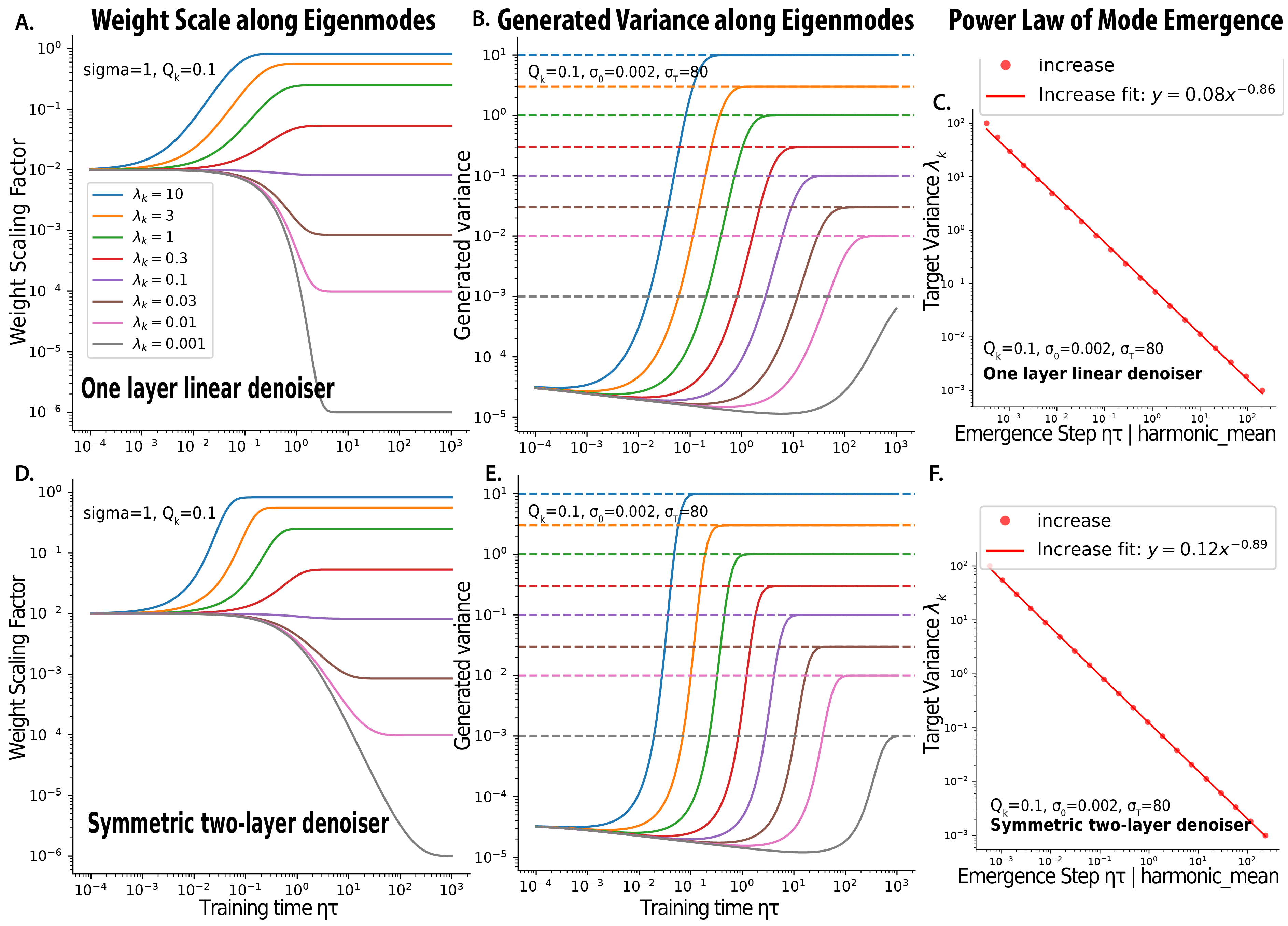
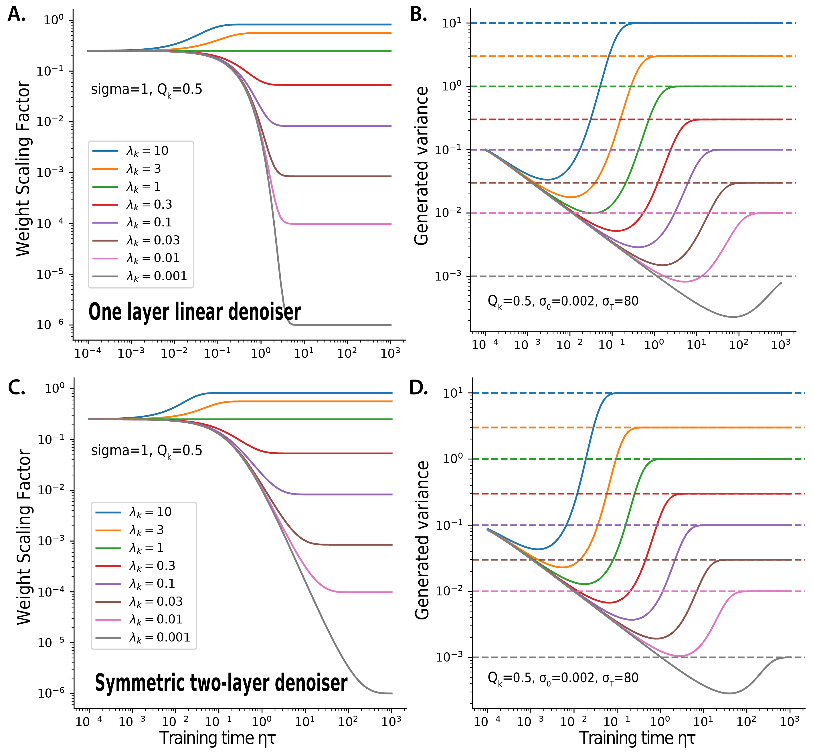
Figure 2: Learning dynamics of the weight and variance of the generated distribution per eigenmode. Top: one-layer linear denoiser, Bottom: two-layer symmetric denoiser. A.D. Learning dynamics of weights $\mathbf{u}_{k}^{\intercal}\mathbf{W}(\tau)\mathbf{u}_{k}$ ($\sigma=1$). B.E. Learning dynamics of the variance of the generated distribution $\tilde{\lambda}_{k}$, as a function of the variance of the target eigenmode $\lambda_{k}$. C.F. Power law between mode emergence time $\tau^{*}_{k}$ and target variance $\lambda_{k}$.

4.1 Zero-Mean Case: Mode-by-mode Exponential Convergence

Consider a single noise scale $\sigma$, when the data has zero mean, $\bm{\mu}=0$, then the DSM gradients simplify to

$\displaystyle\nabla_{\mathbf{W}}\,\mathcal{L}_{\sigma}$ $\displaystyle\;=\;2\,\bigl{[}\mathbf{W}(\sigma^{2}\mathbf{I}+\bm{\Sigma})\;-\;\bm{\Sigma}\bigr{]},\qquad$ (20)
$\displaystyle\nabla_{\mathbf{b}}\,\mathcal{L}_{\sigma}$ $\displaystyle\;=\;2\,\mathbf{b}.$ (21)

which decouples the dynamics of $\mathbf{W}$ and $\mathbf{b}$. Projecting onto the eigenbasis of $\bm{\Sigma}$, the gradient flow ODEs admit closed form solutions:

$\displaystyle\mathbf{b}(\tau)$ $\displaystyle=\mathbf{b}(0)\,e^{-2\eta\tau},$ (22)
$\displaystyle\mathbf{W}(\tau)$ $\displaystyle=\mathbf{W}^{*}+\sum_{k=1}^{d}\bigl{(}\mathbf{W}(0)-\mathbf{W}^{*}\bigr{)}\mathbf{u}_{k}\mathbf{u}_{k}^{\intercal}\,e^{-2\eta\tau(\sigma^{2}+\lambda_{k})}$
Remark 4.1.

Each eigenmode converges exponentially at a rate proportional to $(\sigma^{2}+\lambda_{k})$. This shows, 1) for the same eigenmode, the weights at larger noise scale $\sigma$ will converge faster; 2) for the same noise scale $\sigma$, weights $\mathbf{W}$ will converge faster along modes with larger eigenvalues $\lambda_{k}$. Further, for modes with variance $\lambda_{k}\ll\sigma^{2}$ much smaller than noise, they are effectively “un-resoved” from the noise, and they will converge at similar speed as the noise floor. This effect can be observed in weight scaling curve (Fig. 2A,6A), where weight along lower eigenmodes converge at the same speed.

4.2 General Case: Interaction of Mean and Covariance Learning

In real life, even after pre-processing, dataset mean is not zero, for example, mean of human face distribution is an “average face” (Langlois & Roggman, 1990). So it’s interesting to consider the non-zero mean case analytically. When $\mu\neq 0$, the gradients to $\mathbf{W}$ and $\mathbf{b}$ become interdependent (7), resulting in a coupled linear dynamic system as follows.

Proposition 4.2.

Gradient flow (11) is equivalent to the following ODE, with redefined dynamic variables, $\mathbf{v}_{k}(\tau)=\mathbf{W}(\tau)\mathbf{u}_{k}$, $\bar{\mathbf{b}}(\tau)=\mathbf{b}(\tau)-\mu$. Denote overlap $m_{k}:=\mathbf{u}_{k}^{\intercal}\mathbf{\mu}$,

$\displaystyle\frac{1}{2\eta}\frac{d}{d\tau}\Bigg{[}\begin{array}[]{c}\mathbf{v}_{1}\\ \mathbf{v}_{2}\\ .\\ \bar{b}\end{array}\Bigg{]}=-M\Bigg{[}\begin{array}[]{c}\mathbf{v}_{1}\\ \mathbf{v}_{2}\\ .\\ \bar{b}\end{array}\Bigg{]}+\Bigg{[}\begin{array}[]{c}\lambda_{1}\mathbf{u}_{1}\\ \lambda_{2}\mathbf{u}_{2}\\ .\\ 0\end{array}\Bigg{]}$ (35)

with a fixed dynamic matrix $M$ defined by $\otimes$ tensor product.

$\displaystyle M$ $\displaystyle:=\begin{bmatrix}\sigma^{2}+\lambda_{1}+m_{1}^{2}&m_{1}m_{2}&\quad.\quad&m_{1}\\ m_{1}m_{2}&\sigma^{2}+\lambda_{2}+m_{2}^{2}&\quad.\quad&m_{2}\\ ...&...&...&.\\ m_{1}&m_{2}&.&1\end{bmatrix}\otimes I_{d}$
$\displaystyle:=\tilde{M}\otimes I_{d}$ (36)
Remark 4.3.

The symmetric matrix $\tilde{M}$ (4.2) has a rank-one plus diagonal structure, eigenvalues of such matrix can be found efficiently by numerical algebra, with eigenvectors expressed by Bunch–Nielsen–Sorensen formula (Bunch et al., 1978; Gu & Eisenstat, 1994). Without closed form formula, we’d resort to qualitative analysis and low dimensional examples to gain further insights. We can see the coupling of $\mathbf{W}$ and $\mathbf{b}$ dynamics comes from the overlap of mean and covariance $m_{k}$. When $\mathbf{u}_{k}^{\intercal}\mu=0$, then the dynamics of the corresponding weight projection $\mathbf{v}_{k}(\tau)$ will be the same as the zero mean case, i.e. exponentially convergence to the optimal solution. When $\mathbf{u}_{k}^{\intercal}\mu\neq 0$, the overlap between the distribution mean and and covariance PC will induce coupled linear dynamics between $\mathbf{v}_{k}(\tau)$ and $\mathbf{b}(\tau)$, which could be non-monotonic.

Two dimensional example

Here, we’d show a low dimensional example for the interaction between distribution mean and one eigenmode in the weight. Consider the case where distribution mean $\mu$ lies on the direction of a PC $\mathbf{u}_{k}$. Then only the $\mathbf{u}_{k}$ mode of weights interacts with the distribution mean, resulting in a two-dimensional linear system, parametrized by noise scale $\sigma$, variance of mode $\lambda$ and amount of alignment $m$. Let dynamic variable be scalars $w,b$, $\mathbf{v}_{k}=w(\tau)\mathbf{u}_{k},\mathbf{b}=b(\tau)\mathbf{u}_{k}$.

$\displaystyle\frac{1}{2\eta}\frac{d}{d\tau}\begin{bmatrix}w\\ b\end{bmatrix}=-\begin{bmatrix}m^{2}+\sigma^{2}+\lambda&m\\ m&1\end{bmatrix}\begin{bmatrix}w\\ b\end{bmatrix}+\begin{bmatrix}\lambda+m^{2}\\ m\end{bmatrix}$

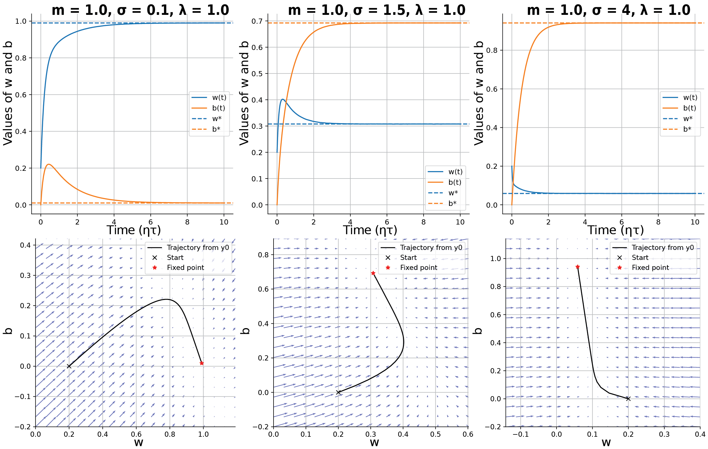
The phase diagram and dynamics depending on the noise scale are showed (Fig. 3): At larger $\sigma$ values, the dynamics of weights $w$ will be much faster than $b$, basically, $w$ gets dynamically captured by $b$, while $b$ slowly relaxed to the optimal value. At small $\sigma$ values, the dynamics timescale of $w$ and $b$ will be closer to each other, and $b$ will usually have non-monotonic transient dynamics. When $\sigma^{2}$ and $\lambda$ are comparable, $w$ will have non-monotonic dynamics.

Refer to caption

Figure 3: Interaction of mean and covariance learning. Top solution to the $w,b$ dynamics under different noise level $\sigma\in\{0.1,1.5,4\}$. Bottom Phase portraits corresponding to the two-d system. ($m=1,\lambda_{k}=1$)

4.3 Learning Dynamics of Sampled Distribution

Next, we leveraged the machinery in Sec. 3.4 to compute the sampled distribution at training time $\tau$, esp. for zero-mean $\bm{\mu}=0$ case. Consider the solution to the weights (22), when the weight initialization $\mathbf{W}(0;\sigma)$ aligns with eigenbasis, then the solution $\mathbf{W}(\tau;\sigma)$ will stay aligned with the basis, through training and noise scale.

Proposition 4.4 (Dynamics of generated distribution in one layer case).

Assume aligned weight initialization, homogeneous across noise scales $\mathbf{W}(0;\sigma)=\sum_{k}Q_{k}\mathbf{u}_{k}\mathbf{u}_{k}^{\intercal}$; Assume independent gradient flow dynamics with the same learning rate $\eta$ of weights at each scale, then during training, the sampled distribution $p(\mathbf{x}_{0};\tau)$ by solving PF-ODE from $\sigma_{T}$ to $\sigma_{0}$ can be expressed as $\mathcal{N}(\tilde{\mu},\tilde{\bm{\Sigma}})$, $\tilde{\bm{\Sigma}}=\sum_{k}\tilde{\lambda}_{k}(\tau)\mathbf{u}_{k}\mathbf{u}_{k}^{\intercal}$ with variance $\tilde{\lambda}_{k}(\tau)=\sigma_{T}^{2}\Phi_{k}^{2}(\sigma_{0})/\Phi_{k}^{2}(\sigma_{T})$

$\displaystyle\Phi_{k}(\sigma)$ $\displaystyle=\sqrt{\lambda_{k}+\sigma^{2}}\exp\bigg{(}\frac{1}{2}\bigg{[}(1-Q_{k})\,\operatorname{Ei}\left(-2\eta\tau\sigma^{2}\right)e^{-2\eta\tau\lambda_{k}}$
$\displaystyle\quad-\operatorname{Ei}\left(-2\eta\tau\left(\sigma^{2}+\lambda_{k}\right)\right)\bigg{]}\bigg{)}$ (37)
Remark 4.5.

To gain further insights, we showed the training dynamics of the variance of generated distribution $\tilde{\lambda}_{k}$ along each eigenmode as a function of variance of the mode. ($Q_{k}=0.1$, Fig. 2B, for other $Q_{k}$ values, see Fig. 6B). Basically, all modes start with similar variance determined by the weight initialization $Q_{k}$ and integration limit $\sigma_{0},\sigma_{T}$ of PF-ODE, then they converged to the correct variance following sigmoidal dynamics, mode by mode. Importantly, the convergence time of each mode follows an inverse power law with the target variance, $\tau_{k}^{*}\propto\lambda_{k}^{-\alpha}$, $\alpha\approx 1$ (Fig. 2C). Here we quantified the convergence time as the first time that the generated variance $\tilde{\lambda}$ reached the harmonic or geometric mean between the initial and target variance. When weight initialization $Q_{k}$ is larger, the initial sampling variance will be higher, the modes decreasing their variance and those increasing their variance will follow separate inverse power laws, with somewhat different exponents (Fig. 7).

Remark 4.6 (Implication).

This shows that, when diffusion training stops earlier, the generated distribution $p(\tilde{\mathbf{x}})$ would have converged to the correct variance along the top eigenmodes, but have not in the lower eigenmodes, namely a spectral bias towards the top eigenmodes during training. Specially, modes with 1/10 variance would require 10 times more training time or samples to learn! In practice, some lower eigenmodes represent noise and are not critical, while others, despite accounting for only a small fraction of the total variance, can be crucial for perception—such as the fine details of human fingers in a portrait.

5 Two-Layer Linear Networks

5.1 Symmetric Parameterization $P\,P^{\intercal}$

Now for each noise scale $\sigma$, consider a two-layer linear denoiser architecture with symmetric weights,

$\displaystyle\mathbf{D}(\mathbf{x};\sigma)\;=\;P\,P^{\intercal}\,\mathbf{x}\;+\;\mathbf{b}.$ (38)

When the data has zero mean ($\mu=0$), the gradient of the DSM objective with respect to parameter $P$ remains tractable, $\nabla_{P}\mathcal{L}_{\sigma}$. (Appendix D). Represent the weight $P$ by its projection in the eigenmode $q_{k}:=P^{\intercal}\mathbf{u}_{k}$, then its gradient has an explicit form

$\displaystyle\nabla_{q_{k}}\mathcal{L}_{\sigma,\mu=0}$ $\displaystyle=-4\lambda_{k}q_{k}+2\sum_{m}\big{(}2\sigma^{2}+\lambda_{m}+\lambda_{k}\big{)}(q_{k}^{\intercal}q_{m})q_{m}$

When $q_{k}$ are initialized orthogonally to each other $q_{k}^{\intercal}(0)q_{m}(0)=0$, one obtains an independent ODE of $q_{k}$

$\displaystyle\frac{dq_{k}}{d\tau}$ $\displaystyle=4\eta(\lambda_{k}-\big{(}\sigma^{2}+\lambda_{k}\big{)}(q_{k}^{\intercal}q_{k}))q_{k}$ (39)

Although this is a non-linear ODE, it admits a close-form solution of $q_{k}$. This type of nonlinear dynamics have been noted more generally in many previous works examining deep linear networks learning dynamics (Saxe et al., 2013; Fukumizu, 1998; Atanasov et al., 2021).

Proposition 5.1 (Dynamics of weight in two layer linear model (aligned initialization)).

Assume centered data $\mu=0$; Assume the weight matrix is initialized aligned to the eigenbasis of data, i.e. $\mathbf{u}_{i}^{\intercal}P(0;\sigma)P(0;\sigma)^{\intercal}\mathbf{u}_{j}=0,\forall i\neq j$, then the gradient flow ODE admits a closed-form solution for the weight at noise scale $\sigma$

$\displaystyle W(\tau;\sigma)$ $\displaystyle=P(\tau;\sigma)P(\tau;\sigma)^{\intercal}=\sum_{k}\|q_{k}(\tau)\|^{2}\mathbf{u}_{k}\mathbf{u}_{k}^{\intercal}$ (40)
$\displaystyle=\sum_{k}\frac{\lambda_{k}}{\sigma^{2}+\lambda_{k}}$ $\displaystyle\mathbf{u}_{k}\mathbf{u}_{k}^{\intercal}\bigg{(}\frac{\|q_{k}(0)\|^{2}}{(\frac{\lambda_{k}}{\sigma^{2}+\lambda_{k}}-\|q_{k}(0)\|^{2})e^{-8\eta\lambda_{k}\tau}+\|q_{k}(0)\|^{2}}\bigg{)}$

When no mode has zero initialization $\|q_{k}(0)\|\neq 0,\forall k$, it asymptotically converges to the same weights $\mathbf{W}^{*}$ as in the one-layer case, $\lim_{\tau\to\infty}P(\tau;\sigma)\,P(\tau;\sigma)^{\intercal}\;\to\;\bm{\Sigma}(\bm{\Sigma}+\sigma^{2}\mathbf{I})^{-1}$.

Remark 5.2.

In two layer network, the magnitude of each mode follows sigmoidal dynamics. Instead of exponential convergence in the original space, it follows exponential convergence on the reciprocal space, with rate $8\eta\lambda_{k}$, which is directly proportional to the variance of the mode. Comparing to the single layer case (Fig. 2 D vs A), modes with larger eigenvalues will converge faster and sharper, while modes with variances smaller than $\sigma^{2}$ will converge at slower speed, since they do not have the flooring effect of $\sigma^{2}$ as in the one layer case. The emergence time of each mode in the weight is inversely proportional to $\lambda_{k}$

$$\tau^{*}(\lambda_{k})=\frac{\ln 2}{8\,\eta\,\lambda_{k}}$$ (41)

when the magnitude of the mode $\|q_{k}(\tau)\|^{2}$ reached the harmonic mean between the initial and asymptotic value.

Remark 5.3 (Qualitative analysis of general initialization).

Even when the weights are initialized from small random values, the analytical solution above will be good approximation to the actual gradient flow (Saxe et al., 2013). More general, for non-aligned initialization $\mathbf{u}_{i}^{\intercal}P(0;\sigma)P(0;\sigma)^{\intercal}\mathbf{u}_{j}\neq 0$, we performed a qualitative analysis of its dynamics in Appendix D.1.2. Basically, eigenmodes with higher variance will converge first with sigmoidal dynamics; then the overlap i.e. off diagonal values will follow non-monotonic rise-and-fall dynamics, and subsequently the eigenmodes with smaller variance will rise with sigmoidal dynamics. Similar results have also been noted in recent works on deep linear networks (Dominé et al., 2023)(Fig.4).

5.2 Learning Dynamics of Sampled Distribution

As before, the sampling ODE

$\displaystyle\frac{d}{d\sigma}\mathbf{x}=-\frac{1}{\sigma}\Bigl{[}P(\tau;\sigma)\,P(\tau;\sigma)^{\intercal}\,\mathbf{x}\;-\;\mathbf{x}\Bigr{]}$ (42)

can be integrated exactly once $P(\tau;\sigma)$ is known in closed form for each noise scale $\sigma$. This is especially illuminating when the $P$ matrices were initialized small or diagonalizable by the covariance eigenbasis. If so, the $P(\tau;\sigma)P(\tau;\sigma)^{\intercal}$ will stay digonalizable with the eigenbasis across $\tau$ and $\sigma$. Then the sampling ODE can be solved mode by mode by projecting onto the eigenbasis $c_{k}(\sigma)=\mathbf{u}^{\intercal}_{k}\mathbf{x}(\sigma)$.

Proposition 5.4 (Dynamics of generated distribution in two layer case).

Assume centered data $\mu=0$; Assume aligned weight initialization, homogeneous across noise scales $P(0;\sigma)P(0;\sigma)^{\intercal}=\sum_{k}Q_{k}\mathbf{u}_{k}\mathbf{u}_{k}^{\intercal}$; Assume independent gradient flow dynamics with the same learning rate $\eta$ of weights at each scale; then during training, the sampled distribution $p(\mathbf{x}_{0};\tau)$ by solving PF-ODE from $\sigma_{T}$ to $\sigma_{0}$ can be expressed as $\mathcal{N}(\tilde{\mu},\tilde{\bm{\Sigma}})$, $\tilde{\bm{\Sigma}}=\sum_{k}\tilde{\lambda}_{k}(\tau)\mathbf{u}_{k}\mathbf{u}_{k}^{\intercal}$ with variance $\tilde{\lambda}_{k}(\tau)=\sigma_{T}^{2}\Phi_{k}^{2}(\sigma_{0})/\Phi_{k}^{2}(\sigma_{T})$

$\displaystyle\Phi_{k}(\sigma)=$ $\displaystyle(\sigma)^{\frac{(1-Q_{k})e^{-8\eta\tau\lambda_{k}}}{Q_{k}+(1-Q_{k})e^{-8\eta\tau\lambda_{k}}}}\times$ (43)
$\displaystyle\bigg{[}\lambda_{k}e^{-8\eta\tau\lambda_{k}}$ $\displaystyle+Q_{k}\left(1-e^{-8\eta\tau\lambda_{k}}\right)\left(\lambda_{k}+\sigma^{2}\right)\bigg{]}^{\frac{Q_{k}}{2Q_{k}+2(1-Q_{k})e^{-8\eta\tau\lambda_{k}}}}$
Remark 5.5.

We visualized the learning dynamics of distribution in Fig. 2E: similar to the single layer case, the variance of generated distribution converges to the target one mode by mode with sigmoidal dynamics, following the descending order of variance. The convergence time also follows inverse power law with the variance $\lambda_{k}$ (Fig. 2F). When the initialization $Q_{k}$ is larger, some eigenmodes will have higher initial variance, causing their generated variance to first decay and then converge sigmoidally to the target (Fig. 6). Comparing two layer to one layer linear network, even though their expressivity do not change, the exponents in the scaling law of mode emergence time differ (Fig. 7).

6 Empirical Validation of the Theory in Practical Diffusion Model Training

To demonstrate real-world applicability, we trained diffusion models under progressively realistic conditions.

6.1 General Experimental Approach

To test our theory, we resort to the following general methodology: 1) we fix a training dataset $\{\mathbf{x}_{i}\}$ and compute its empirical mean $\bm{\mu}$ and covariance $\bm{\Sigma}$. We then perform an eigen-decomposition of $\bm{\Sigma}$, obtaining eigenvalues $\lambda_{k}$ and eigenvectors $\mathbf{u}_{k}$. 2) Next, we train a diffusion model on this dataset by optimizing the DSM objective with a neural network denoiser $\mathbf{D}_{\theta}(\mathbf{x},\sigma)$. 3) During training, at certain steps $\tau$, we generate samples $\{\mathbf{x}_{i}^{\tau}\}$ from the diffusion model by integrating the PF-ODE (Eq. 1). We then estimate the sample mean $\tilde{\bm{\mu}}^{\tau}$ and sample covariance $\tilde{\bm{\Sigma}}^{\tau}$. To evaluate convergence, we measure the deviation of the generated sample mean from the true mean, $\tilde{\bm{\mu}}^{\tau}-\bm{\mu}$, and project their deviation onto the eigenbasis $\mathbf{u}_{k}^{\intercal}(\tilde{\bm{\mu}}^{\tau}-\bm{\mu})$. Finally, we compute the variance of the generated samples along the eigenbasis of training data, $\tilde{\lambda}_{k}^{\tau}=\mathbf{u}_{k}^{\intercal}\tilde{\bm{\Sigma}}^{\tau}\mathbf{u}_{k}$. To stress test our theory and maximize its relevance, we’d keep most of the training hyperparameters as practical ones.

6.2 Multi-Layer Perceptron (MLP)

Refer to caption

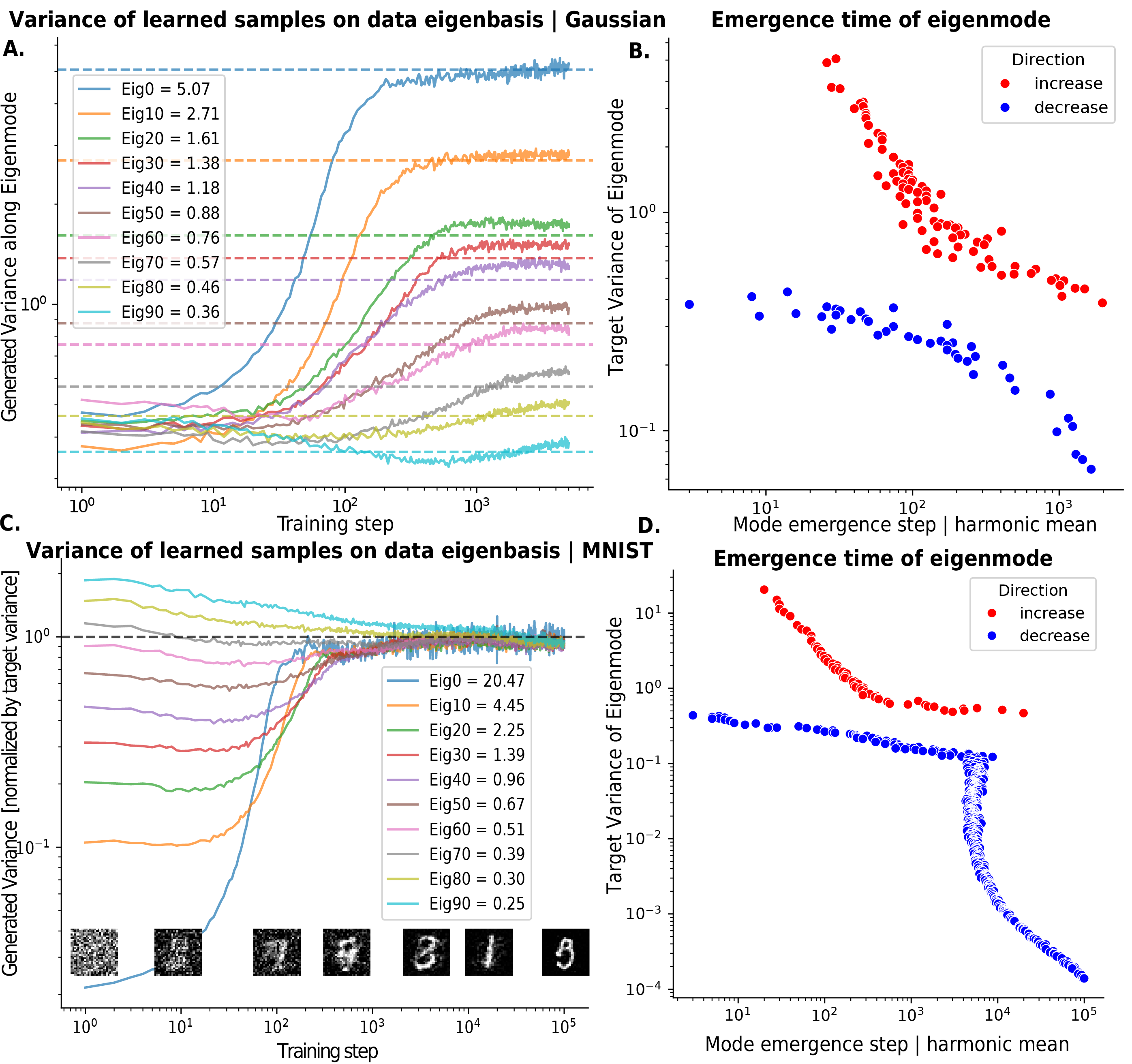
Figure 4: Validation experiment with MLP. Top row. Gaussian data, 128d A. Variance of generated samples along eigenmodes $\tilde{\lambda}_{k}^{\tau}$ throughout learning. B. Mode emergence time as a function of variance of target eigenmode $\lambda_{k}$. Bottom row. MNIST data, C. Generated variance normalized by target variance $\tilde{\lambda}_{k}^{\tau}/\lambda_{k}$ throughout learning as a function of eigenmode $k$. Samples generated from training steps were annotated along the x-axis. D. Mode emergence time as a function of variance of target eigenmode.

We used a Multi-Layer Perceptron (MLP) inspired by the SongUnet-like network in EDM (Song et al., 2021; Karras et al., 2022). We found this architecture effective in learning distribution like point cloud data (Fig. 15). We kept the preconditioning and weights the same as in (Karras et al., 2022). The specific design can be found in Appendix F.1.

Experiment 1: Zero-mean Gaussian Data x MLP

We first consider a zero mean Gaussian $\mathcal{N}(\mathbf{0},\bm{\Sigma})$ as training distribution, with covariance defined as a randomly rotated diagonal matrix with log normal spectrum. We modeled them with MLPs with 5 block and 256 dims. The experiment details can be found in Appendix F.3.

We tracked the evolution of the variance of sampled distribution along eigenbasis of training data $\tilde{\lambda}_{k}(\tau)$ (Fig. 4A). We can see the variance of each eigenmodes converge with sigmoidal dynamics to the target value $\lambda_{k}$, with higher variance modes converging faster. We quantified the emergence time $\tau^{*}$ as in our theory – the step reaching the harmonic mean of initial and asymptotic variance (Fig. 4B). Quantitatively, we found the convergence time of top eigenmodes follow the inverse power law nicely, with exponent close to $-1$. However, this relation breaks down when target variance gets closer to the initial variance of the mode. For modes with decreasing variance, it also follows an inverse law relation with different exponent, reminiscent of $Q_{k}=0.5$ case in Fig. 7. This experiment shows that despite many non-idealistic conditions e.g. deeper network, nonlinear activation function, residual connections, normal weights initialization, coupled parametrization of network at different noise, the prediction from the linear spectral theory is still qualitatively correct.

Experiment 2: Natural Image Datasets x MLP

Most data that are interesting enough to be modeled do not follow a Gaussian distribution. So, we asked, is Gaussian data a necessary condition for the theory to work? We tested it on natural image data, which is not globally Gaussian. We flattened MNIST images as 768 dim vectors and model them with deeper and wider MLPs (8 block, 1024 dim).

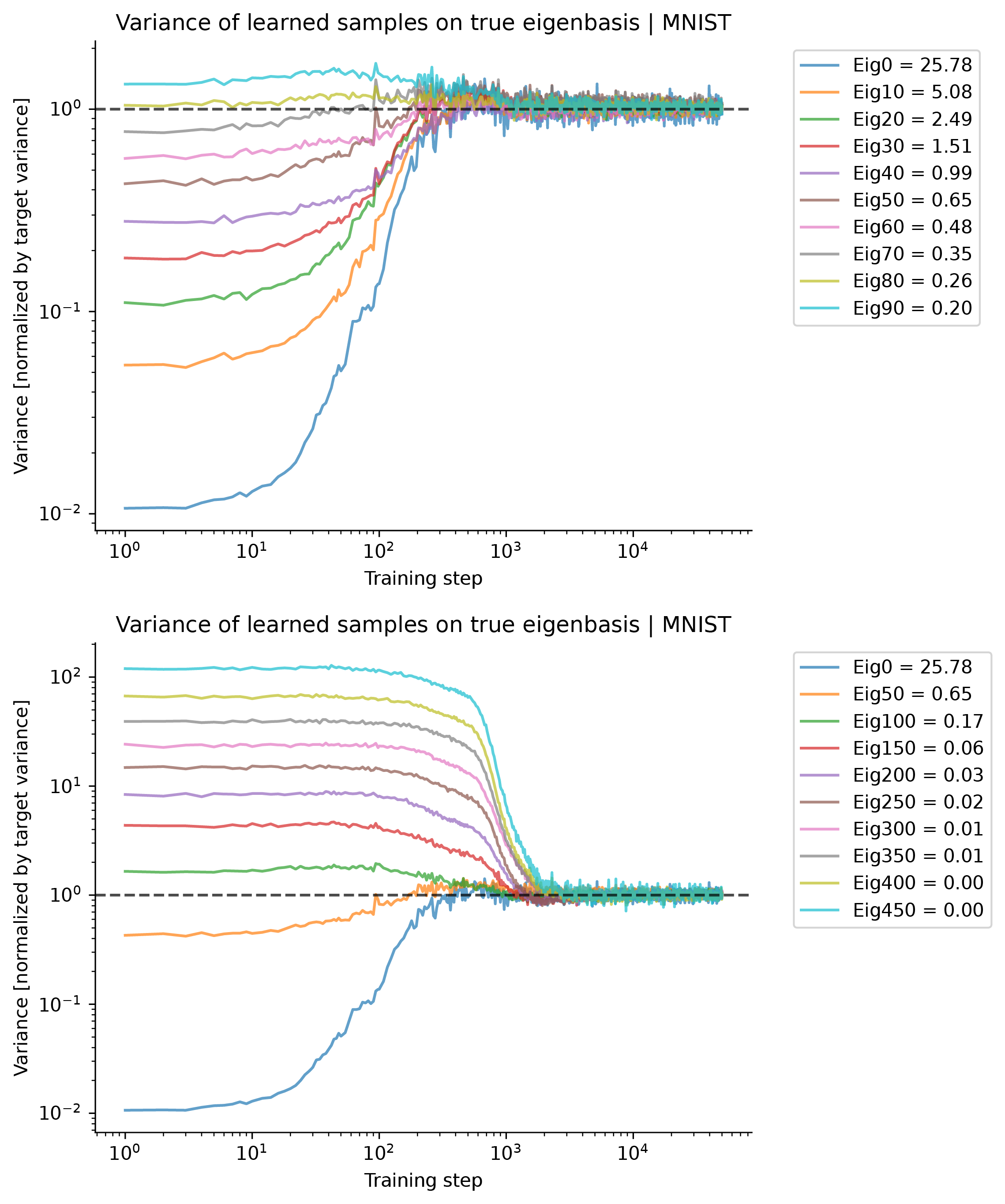
We found consistent results with Gaussian data: mode variance converges with sigmoidal dynamics to the target (Fig. 4C). Quantitatively, the emergence time $\tau^{*}$ of top eigenvalues follow a power law, and modes with smaller variance follow a different power law, with smallest eigenmodes converged at last (Fig. 4D). This shows, even when the point cloud to be modeled is not Gaussian, the learning dynamics of MLP based diffusion model are still dominated by the Gaussian spectral structure.

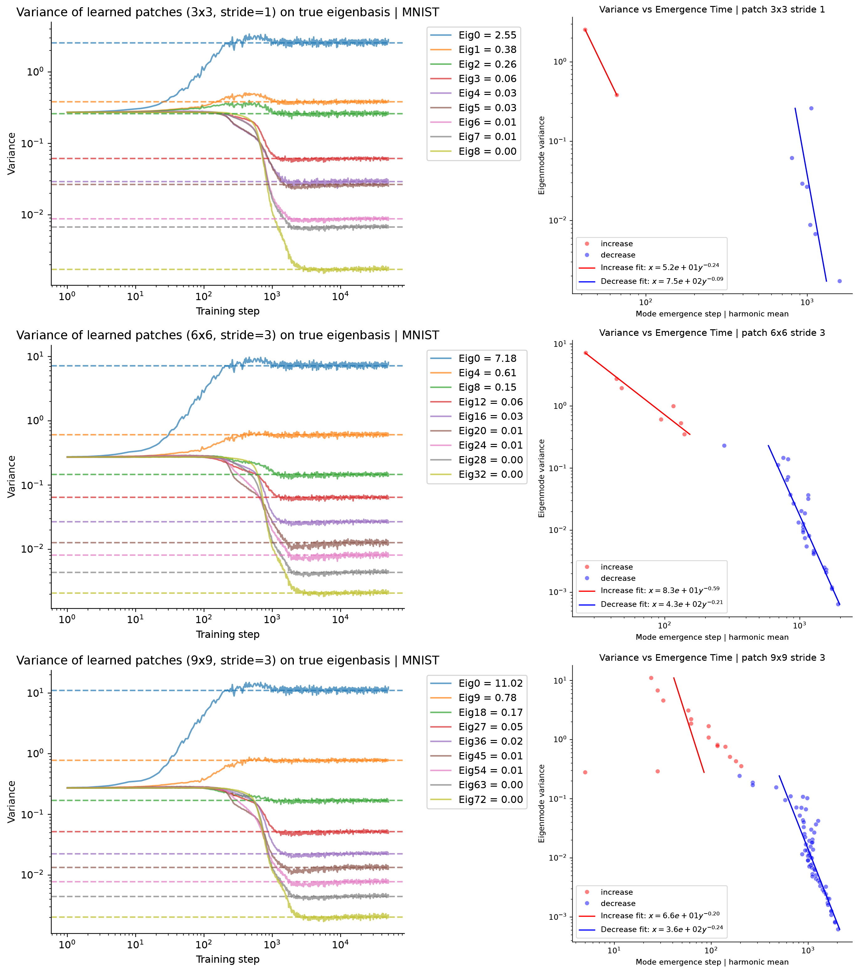
6.3 Convolutional Neural Networks (CNNs)

Refer to caption

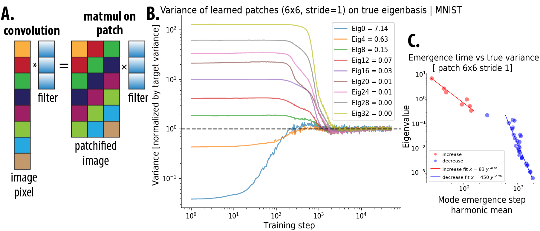
Figure 5: Spectral Bias in Patch of CNN learning — MNIST A. Schematics showing the equivalence of convolution on image and matrix multiplication on stacked patches. B. Training dynamics of patch variance along eigenbasis (normalized by target variance). C. Emergence time vs target variance of patch eigenmode.

For structured data like natural images, neural networks with stronger inductive bias will be preferred over MLPs. Specifically, UNet (Ronneberger et al., 2015) with convolutional layers and potentially self-attention layers is commonly used as score approximator in natural image modeling (Song et al., 2021). So, we tested whether our theory of spectral bias in learning holds for convolutional neural network (CNN) based UNet.

Experiment 3: Natural Image Datasets x CNN UNet

First, we found that naively applying the theory will not correctly predict the evolution of generated data covariance, as modes with different variance will emerge at roughly the same time (Fig. 10). We hypothesized that this is due to the interaction between the inductive bias of the CNN and the data spectrum. It’s well known that convolution can be equivalently thought of as kernel weights applying to patches of the image (Fig. 5A). Thus from the eyes of the kernels, the data distribution is not that of the whole image, but that of image patches.

Thus, we again tested our theory in the domain of patches. For images, we extracted patches with certain size and stride; then we computed the mean and covariance of patches extracted from training data; and examined the mean and covariance of patches from the generated data. We found from the eyes of patches, the prediction of the theory is more valid (Fig. 5B). Further, this is not limited to the kernel size of the first convolution layer ($3\times 3$, stride 1); even for larger patch sizes like $6\times 6$, the prediction from theory still holds.

7 Discussion

In summary, we presented closed-form solutions for training linear denoisers (or, linear score networks) under the DSM objective on arbitrary data. This setup allows for a precise mode-wise understanding of the gradient flow dynamics of the denoiser and the training dynamics of the learned distribution. For both the weights and the distribution, we showed analytical evidence of spectral bias, i.e. weights converge faster along the eigenmodes with high variance, and the learned distribution recovers the true variance first along the top eigenmodes. We hope these results can serve as a pedagogical model for spectral bias in the diffusion models through the interaction of training and sampling. Furthermore, our analysis is not limited to the diffusion model and the denoising score matching loss. 
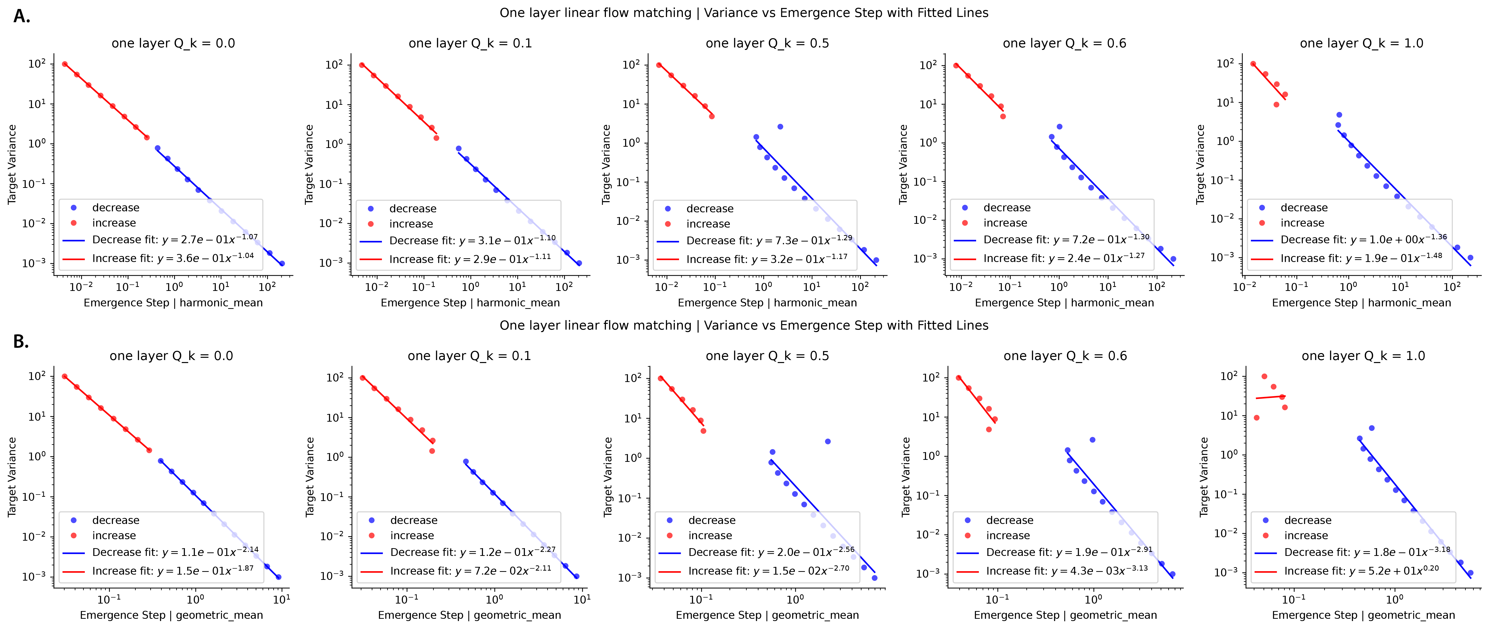
In Appendix E, we showed a similar derivation for the spectral bias in flow matching models (Lipman et al., 2022, 2024).

Implication for model training

Further, the demonstrated spectral bias in diffusion learning may be taken into consideration to better precondition the data or the model to accelerate convergence. Our theory predicts to fully learn features of $1/100$ smaller variance, models need to be trained $100$ times longer. We hypothesize that many large scale diffusion models (Rombach et al., 2022; Chen et al., 2023) have not fully converged along some small eigenmodes of the image distributions even when they are released. So our results suggest, by whitening the data and highlighting the variance of certain detail but perceptually critical features (e.g. fingers in human portraits, glass arms), large scale diffusion models may converge faster. Potentially, the autoencoder used in latent diffusion (Rombach et al., 2022) could be used to perform nonlinear whitening.

Relevance of our theoretical assumptions

We found, for the purpose of analytical tractability, we made many idealistic assumptions about neural network training, 1) linear neural network, 2) small or orthogonal weight initialization, 3) “full-batch” gradient flow, 4) independent evolution of weights at each noise scale. In our MLP experiments, we found even when all of these assumptions were somewhat violated, the general theoretical prediction is correct. This shows most of these assumptions could be relaxed in real life, and the spectrum of data had a large effect dominating the learning dynamics.

Inductive bias of the neural network

In our CNN experiments, however, the theoretical prediction is off. The spectral bias on learning speed did not directly apply to the distribution of whole images. We found the theory’s prediction is more relevant when applied to distribution of patches in the training and the generated images. This showed that, the network architecture can have significant effect on the learning dynamics. For CNNs, it’s more properly regarded as linear score model over image patches. Thus for further theoretical work it may be fruitful to consider set ups where networks that have more structure in it (linear convolution (Gunasekar et al., 2018)), which can affect the spectral bias significantly.

Broader Impact

Although our work is primarily theoretical, the inverse scaling law could offer valuable insights into how to improve the training of large-scale diffusion or flow generative models.

Acknowledgements.

We are grateful to Jacob Zavatone-Veth, Cengiz Pehlevan, Yongyi Yang, Michael Albergo, Hugo Cui, Yue Lu, and Ekdeep Lubana for their insightful discussions and valuable pointers to relevant literature. We also thank Thomas Fel for providing formatting code snippet and Zhengdao Chen for meticulously proofreading an early version of the manuscript. This research was supported by the generous funding and computing resources provided by the Kempner Institute at Harvard University.

References

  • Atanasov et al. (2021) Atanasov, A., Bordelon, B., and Pehlevan, C. Neural networks as kernel learners: The silent alignment effect. arXiv preprint arXiv:2111.00034, 2021.
  • Attias & Schreiner (1996) Attias, H. and Schreiner, C. Temporal low-order statistics of natural sounds. Advances in neural information processing systems, 9, 1996.
  • Bordelon et al. (2020) Bordelon, B., Canatar, A., and Pehlevan, C. Spectrum dependent learning curves in kernel regression and wide neural networks. In III, H. D. and Singh, A. (eds.), Proceedings of the 37th International Conference on Machine Learning, volume 119 of Proceedings of Machine Learning Research, pp.  1024–1034. PMLR, 13–18 Jul 2020. URL https://proceedings.mlr.press/v119/bordelon20a.html.
  • Bunch et al. (1978) Bunch, J. R., Nielsen, C. P., and Sorensen, D. C. Rank-one modification of the symmetric eigenproblem. Numerische Mathematik, 31(1):31–48, 1978.
  • Canatar et al. (2021) Canatar, A., Bordelon, B., and Pehlevan, C. Spectral bias and task-model alignment explain generalization in kernel regression and infinitely wide neural networks. Nature Communications, 12(1):2914, May 2021. ISSN 2041-1723. doi: 10.1038/s41467-021-23103-1. URL https://doi.org/10.1038/s41467-021-23103-1.
  • Chen et al. (2023) Chen, J., Yu, J., Ge, C., Yao, L., Xie, E., Wu, Y., Wang, Z., Kwok, J., Luo, P., Lu, H., et al. Pixart-alpha: Fast training of diffusion transformer for photorealistic text-to-image synthesis. arXiv preprint arXiv:2310.00426, 2023.
  • Dhariwal & Nichol (2021) Dhariwal, P. and Nichol, A. Diffusion models beat gans on image synthesis. In Advances in Neural Information Processing Systems (NeurIPS), 2021.
  • Dominé et al. (2023) Dominé, C. C., Braun, L., Fitzgerald, J. E., and Saxe, A. M. Exact learning dynamics of deep linear networks with prior knowledge. Journal of Statistical Mechanics: Theory and Experiment, 2023(11):114004, 2023.
  • Dong & Atick (1995) Dong, D. W. and Atick, J. J. Statistics of natural time-varying images. Network: computation in neural systems, 6(3):345, 1995.
  • Fukumizu (1998) Fukumizu, K. Effect of batch learning in multilayer neural networks. Gen, 1(04):1E–03, 1998.
  • Gu & Eisenstat (1994) Gu, M. and Eisenstat, S. C. A stable and efficient algorithm for the rank-one modification of the symmetric eigenproblem. SIAM journal on Matrix Analysis and Applications, 15(4):1266–1276, 1994.
  • Gunasekar et al. (2018) Gunasekar, S., Lee, J. D., Soudry, D., and Srebro, N. Implicit bias of gradient descent on linear convolutional networks. Advances in neural information processing systems, 31, 2018.
  • Hartman (2002) Hartman, P. Ordinary differential equations. SIAM, 2002.
  • Ho et al. (2020) Ho, J., Jain, A., and Abbeel, P. Denoising diffusion probabilistic models. In Advances in Neural Information Processing Systems (NeurIPS), 2020.
  • Karras et al. (2022) Karras, T., Aittala, M., Aila, T., and Laine, S. Elucidating the design space of diffusion-based generative models. arXiv preprint arXiv:2206.00364, 2022.
  • Langlois & Roggman (1990) Langlois, J. H. and Roggman, L. A. Attractive faces are only average. Psychological science, 1(2):115–121, 1990.
  • Li et al. (2024) Li, X., Dai, Y., and Qu, Q. Understanding generalizability of diffusion models requires rethinking the hidden gaussian structure. arXiv preprint arXiv:2410.24060, 2024.
  • Lipman et al. (2022) Lipman, Y., Chen, R. T., Ben-Hamu, H., Nickel, M., and Le, M. Flow matching for generative modeling. arXiv preprint arXiv:2210.02747, 2022.
  • Lipman et al. (2024) Lipman, Y., Havasi, M., Holderrieth, P., Shaul, N., Le, M., Karrer, B., Chen, R. T., Lopez-Paz, D., Ben-Hamu, H., and Gat, I. Flow matching guide and code. arXiv preprint arXiv:2412.06264, 2024.
  • Pierret & Galerne (2024) Pierret, E. and Galerne, B. Diffusion models for gaussian distributions: Exact solutions and wasserstein errors. arXiv preprint arXiv:2405.14250, 2024.
  • Rahaman et al. (2019) Rahaman, N., Baratin, A., Arpit, D., Draxler, F., Lin, M., Hamprecht, F., Bengio, Y., and Courville, A. On the spectral bias of neural networks. In International Conference on Machine Learning, pp.  5301–5310. PMLR, 2019.
  • Rombach et al. (2022) Rombach, R., Blattmann, A., Lorenz, D., Esser, P., and Ommer, B. High-resolution image synthesis with latent diffusion models. In Proceedings of the IEEE/CVF Conference on Computer Vision and Pattern Recognition, pp.  10684–10695, 2022.
  • Ronneberger et al. (2015) Ronneberger, O., Fischer, P., and Brox, T. U-net: Convolutional networks for biomedical image segmentation. In Medical image computing and computer-assisted intervention–MICCAI 2015: 18th international conference, Munich, Germany, October 5-9, 2015, proceedings, part III 18, pp.  234–241. Springer, 2015.
  • Saxe et al. (2013) Saxe, A. M., McClelland, J. L., and Ganguli, S. Exact solutions to the nonlinear dynamics of learning in deep linear neural networks. arXiv preprint arXiv:1312.6120, 2013.
  • Sohl-Dickstein et al. (2015) Sohl-Dickstein, J., Weiss, E. A., Maheswaranathan, N., and Ganguli, S. Deep unsupervised learning using nonequilibrium thermodynamics. In Proceedings of the 32nd International Conference on Machine Learning (ICML), 2015.
  • Song & Ermon (2019a) Song, Y. and Ermon, S. Generative modeling by estimating gradients of the data distribution. In Wallach, H., Larochelle, H., Beygelzimer, A., d'Alché-Buc, F., Fox, E., and Garnett, R. (eds.), Advances in Neural Information Processing Systems, volume 32. Curran Associates, Inc., 2019a. URL https://proceedings.neurips.cc/paper/2019/file/3001ef257407d5a371a96dcd947c7d93-Paper.pdf.
  • Song & Ermon (2019b) Song, Y. and Ermon, S. Generative modeling by estimating gradients of the data distribution. In Advances in Neural Information Processing Systems (NeurIPS), 2019b.
  • Song et al. (2021) Song, Y., Sohl-Dickstein, J., Kingma, D. P., Kumar, A., Ermon, S., and Poole, B. Score-based generative modeling through stochastic differential equations. In International Conference on Learning Representations, 2021. URL https://openreview.net/forum?id=PxTIG12RRHS.
  • Torralba & Oliva (2003) Torralba, A. and Oliva, A. Statistics of natural image categories. Network: computation in neural systems, 14(3):391, 2003.
  • Turk & Pentland (1991) Turk, M. and Pentland, A. Eigenfaces for recognition. Journal of cognitive neuroscience, 3(1):71–86, 1991.
  • Vincent (2011) Vincent, P. A connection between score matching and denoising autoencoders. Neural Computation, 23(7):1661–1674, 2011.
  • Wang & Ponce (2021) Wang, B. and Ponce, C. R. A geometric analysis of deep generative image models and its applications. In International Conference on Learning Representations, 2021. URL https://openreview.net/forum?id=GH7QRzUDdXG.
  • Wang & Vastola (2024) Wang, B. and Vastola, J. The unreasonable effectiveness of gaussian score approximation for diffusion models and its applications. Transactions on Machine Learning Research, December 2024. arXiv preprint arXiv:2412.09726.
  • Wang & Vastola (2023) Wang, B. and Vastola, J. J. The Hidden Linear Structure in Score-Based Models and its Application. arXiv e-prints, art. arXiv:2311.10892, November 2023. doi: 10.48550/arXiv.2311.10892.

Appendix A Extended Results

Refer to caption

Figure 6: Learning dynamics of the weight and variance of the generated distribution per eigenmode (continued) Top Single layer linear denoiser. Bottom Symmetric two-layer denoiser. A.C. Learning dynamics of $\mathbf{u}_{k}^{\intercal}\mathbf{W}(\tau)\mathbf{u}_{k}$. B.D. Learning dynamics of the variance of the generated distribution $\tilde{\lambda}_{k}$, as a function of the variance of the target eigenmode $\lambda_{k}$. This case with larger amplitude weight initialization $Q_{k}=0.5$.

Refer to caption


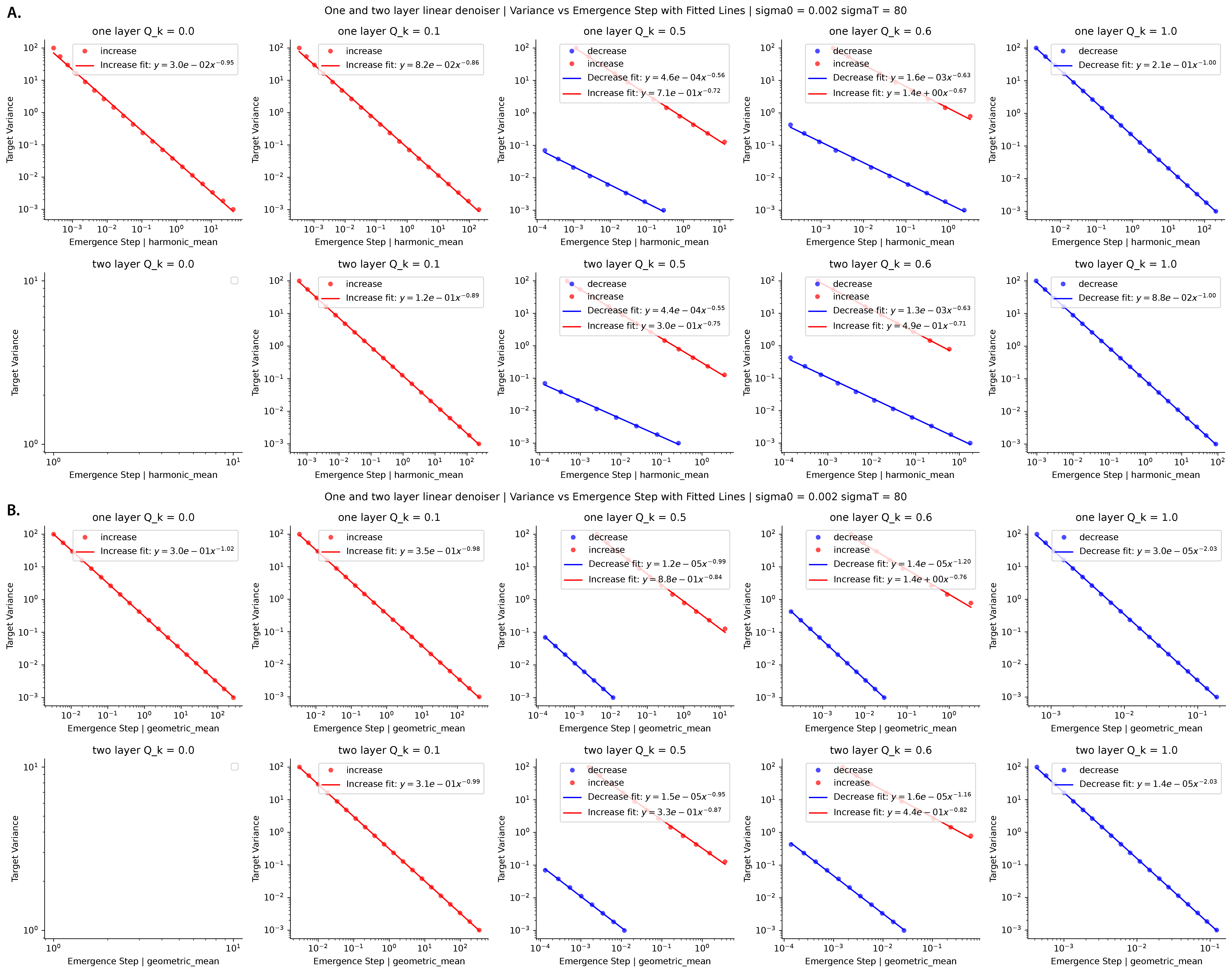
Figure 7: Power law relationship between mode emergence time and target mode variance for one-layer and two-layer linear denoisers. Panels (A) and (B) respectively plot the Mode variance against the Emergence Step for different values of weight initialization $Q_{k}\in\{0.0,\,0.1,\,0.5,\,0.6,\,1.0\}$ (columns), for one layer and two layer linear denoser (rows). We used $\sigma_{0}=0.002$ and $\sigma_{T}=80$. The emergence steps were quantified via different criterions, via harmonic mean in A, and geometric mean in B. Within each panel, red markers and lines denote the modes where their variance increases; blue markers and lines denote modes that “decrease” their variance. The solid lines show least-squares fits on log-log scale, giving rise to the $y=a\,x^{b}$ type relation. Comparisons reveal a systematic power-law decay of variance with respect to the Emergence Step under both the harmonic-mean and geometric-mean definitions. Note, the $Q_{k}=0$ and two layer case was empty since zero initialization is an (unstable) fixed point, thus it will not converge.

Refer to caption

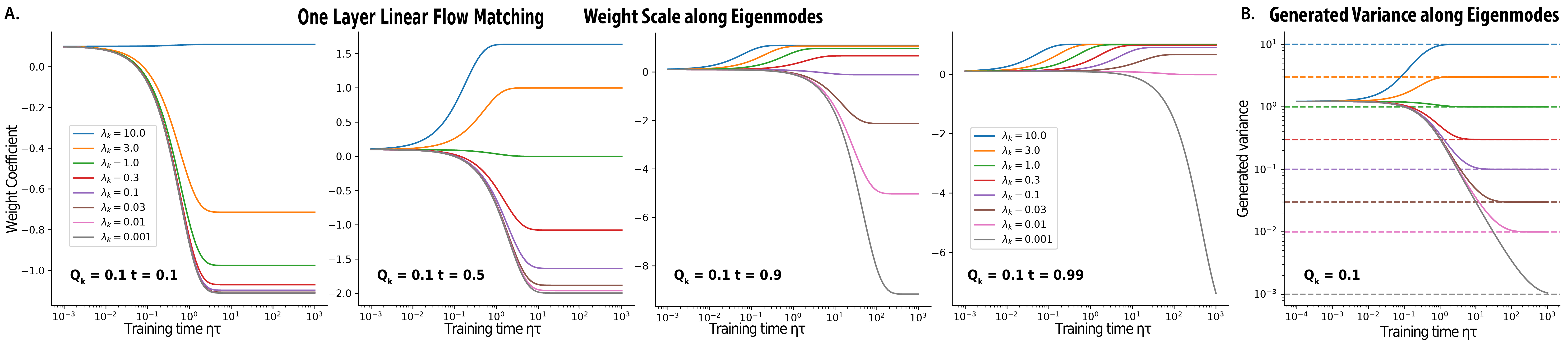
Figure 8: Learning dynamics of the weight and variance of the generated distribution per eigenmode, for one layer linear flow matching model Similar plotting format as Fig. 2. A. Learning dynamics of weights $\mathbf{u}_{k}^{\intercal}\mathbf{W}(\tau;t)\mathbf{u}_{k}$ for various time point $t\in\{0.1,0.5,0.9,0.99\}$. B. Learning dynamics of the variance of the generated distribution $\tilde{\lambda}_{k}$, as a function of the variance of the target eigenmode $\lambda_{k}\in\{10,3,1,0.3,0.1,0.03,0.01,0.001\}$. Weight initialization is set at $Q_{k}=0.1$ for every mode.

Refer to caption

Figure 9: Power law relationship between mode emergence time and target mode variance for one-layer linear flow matching. Panels (A) and (B) respectively plot the Mode variance against the Emergence Step for different values of weight initialization $Q_{k}\in\{0.0,\,0.1,\,0.5,\,0.6,\,1.0\}$ (columns), for one layer linear flow model. The emergence steps were quantified via different criterions, via harmonic mean in A, and geometric mean in B. We used the same plotting format as in Fig. 7. Comparisons reveal a systematic power-law decay of variance with respect to the Emergence Step under both the harmonic-mean and geometric-mean definitions.

Refer to caption

Figure 10: Spectral Bias in Whole Image of CNN learning — MNIST Training dynamics of sample (whole image) variance along eigenbasis of training set, normalized by target variance. Upper 0-100 eigen modes, Lower 0-500 eigenmodes.

Refer to caption

Figure 11: Spectral Bias in CNN-Based Diffusion Learning: Variance Dynamics in Image Patches — MNIST (32 pixel resolution). Left, Raw variance of generated patches along true eigenbases during training. Right, Scaling relationship between the target variance of eigenmode versus mode emergence time (harmonic mean criterion). Each row corresponds to a different patch size and stride used for extracting patches from images.

Refer to caption

Figure 12: Spectral Bias in CNN-Based Diffusion Learning: Variance Dynamics in Image Patches — CIFAR10 (32 pixel resolution). Left, Raw variance of generated patches along true eigenbases during training. Right, Scaling relationship between the target variance of eigenmode versus mode emergence time (harmonic mean criterion). Each row corresponds to a different patch size and stride used for extracting patches from images.

Refer to caption

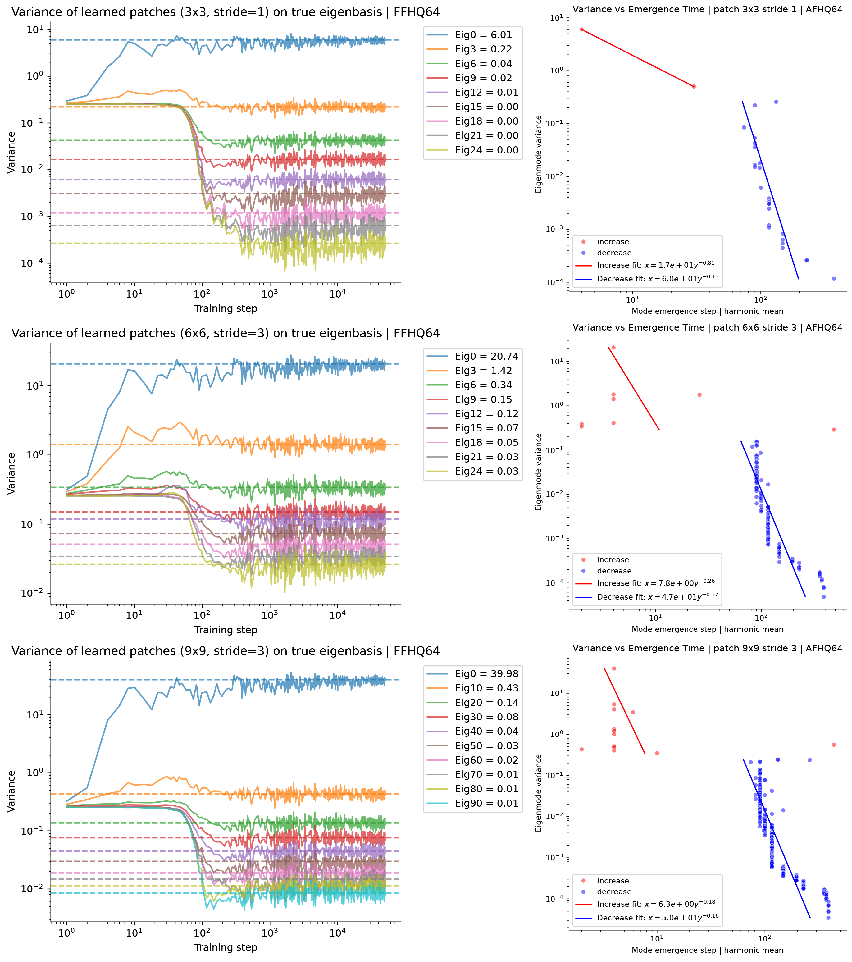
Figure 13: Spectral Bias in CNN-Based Diffusion Learning: Variance Dynamics in Image Patches — FFHQ (64 pixel resolution). Left, Raw variance of generated patches along true eigenbases during training. Right, Scaling relationship between the target variance of eigenmode versus mode emergence time (harmonic mean criterion). Each row corresponds to a different patch size and stride used for extracting patches from images.

Refer to caption

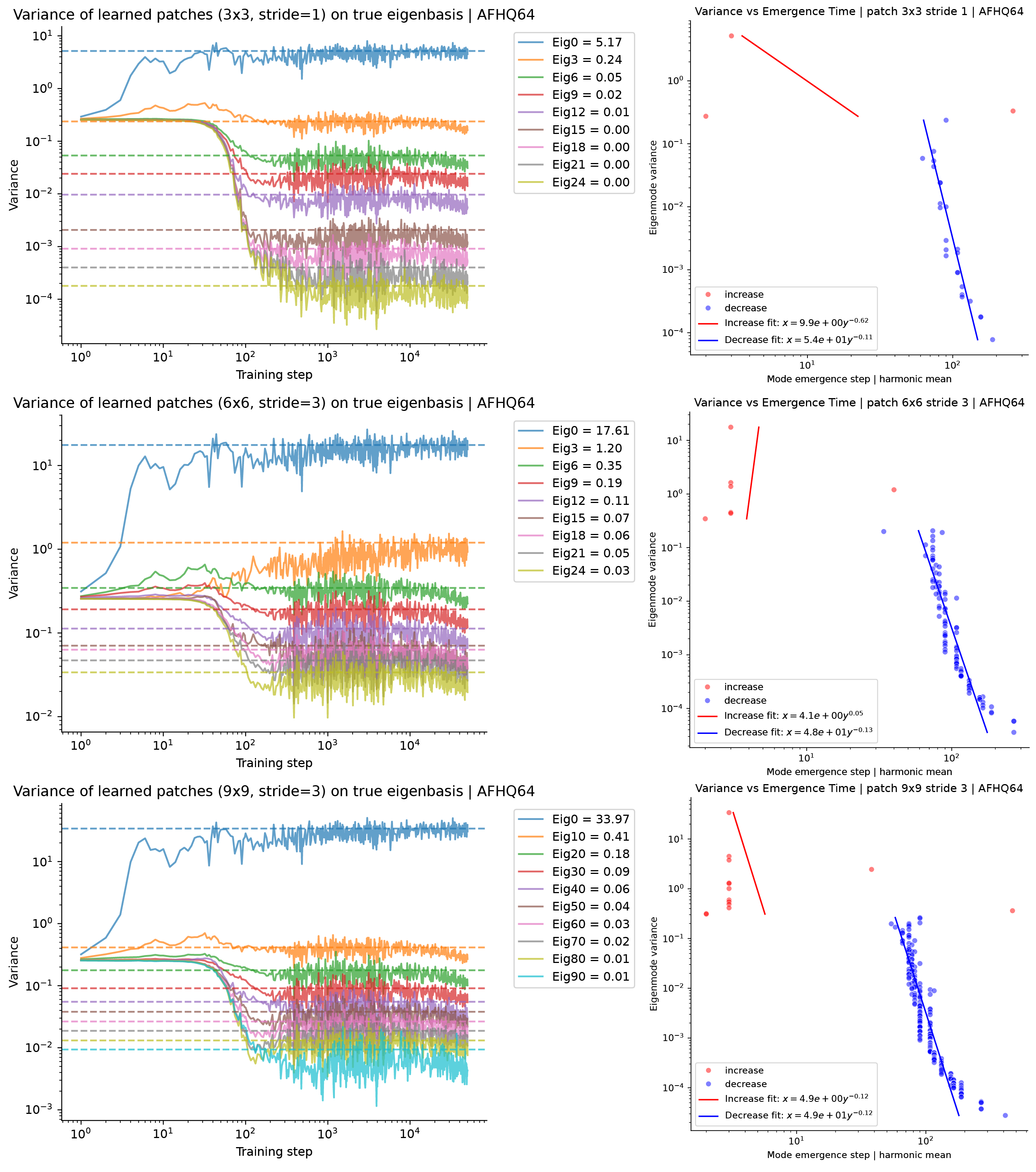
Figure 14: Spectral Bias in CNN-Based Diffusion Learning: Variance Dynamics in Image Patches — AFHQv2 (64 pixel resolution). Left, Raw variance of generated patches along true eigenbases during training. Right, Scaling relationship between the target variance of eigenmode versus mode emergence time (harmonic mean criterion). Each row corresponds to a different patch size and stride used for extracting patches from images.

Appendix B Detailed Derivation: General analysis

B.1 General Analysis of the Denoising Score Matching Objective

To simplify, we first consider a fixed $\sigma$, ignoring the nonlinear dependency on it. Consider our score, denoiser function approximators a linear function $D(\mathbf{x})=b+W\mathbf{x}$. Expanding the DSM loss, we get

$\displaystyle\|\mathbf{D}(\mathbf{x}_{0}+\sigma z;\sigma)-\mathbf{x}_{0}\|^{2}$ $\displaystyle=\|b+W(\mathbf{x}_{0}+\sigma z)-\mathbf{x}_{0}\|^{2}$
$\displaystyle=\|b+W\sigma z+(W-I)\mathbf{x}_{0}\|^{2}$
$\displaystyle=(b+W\sigma z)^{T}(b+W\sigma z)+\mathbf{x}_{0}^{T}(W-I)^{T}(W-I)\mathbf{x}_{0}+2(b+W\sigma z)^{T}(W-I)\mathbf{x}_{0}$
$\displaystyle=b^{T}b+2\sigma b^{T}Wz+\sigma^{2}z^{T}W^{T}Wz+\mathbf{x}_{0}^{T}(W-I)^{T}(W-I)\mathbf{x}_{0}$
$\displaystyle\quad\quad+2b^{T}(W-I)\mathbf{x}_{0}+2\sigma z^{T}W^{T}(W-I)\mathbf{x}_{0}$
$\displaystyle=b^{T}b+2\sigma b^{T}Wz+\sigma^{2}\mbox{Tr}[W^{T}Wzz^{T}]+\mbox{Tr}[(W-I)^{T}(W-I)\mathbf{x}_{0}\mathbf{x}_{0}^{T}]$
$\displaystyle\quad\quad+2b^{T}(W-I)\mathbf{x}_{0}+2\sigma\mbox{Tr}[W^{T}(W-I)\mathbf{x}_{0}z^{T}]$
$\displaystyle=\|b+W(\mathbf{x}_{0}+\sigma z)-\mathbf{x}_{0}\|^{2}$
$\displaystyle=\|b-\mathbf{x}_{0}\|^{2}+\|W(\mathbf{x}_{0}+\sigma z)\|^{2}+2W(\mathbf{x}_{0}+\sigma z)(b-\mathbf{x}_{0})^{T}$
Full batch limit

Note here we can take full batch expectation over $z,\mathbf{x}_{0}$, where $z\sim\mathcal{N}(0,I),\mathbf{x}_{0}\sim p(\mathbf{x}_{0})$, their moments are here.

$\displaystyle\mathbb{E}[z]$ $\displaystyle=0$
$\displaystyle\mathbb{E}[zz^{T}]$ $\displaystyle=I$
$\displaystyle\mathbb{E}[\mathbf{x}_{0}]$ $\displaystyle=\mu$
$\displaystyle\mathbb{E}[\mathbf{x}_{0}\mathbf{x}_{0}^{T}]$ $\displaystyle=\mu\mu^{T}+\Sigma$
$\displaystyle\mathbb{E}[\mathbf{x}_{0}z^{T}]$ $\displaystyle=0$

Note, the data do not need to be Gaussian, as long as the expectations or the first two moments are as computed above, the results should be the same. In a sense, if your function approximator is linear, then you just care about the Gaussian part of data.

$\displaystyle\mathcal{L}=$ $\displaystyle\mathbb{E}_{\mathbf{x}_{0}\sim p_{0}(x),\ z\sim\mathcal{N}(0,I)}\|\mathbf{D}(\mathbf{x}_{0}+\sigma z;\sigma)-\mathbf{x}_{0}\|^{2}$
$\displaystyle=$ $\displaystyle b^{T}b+\sigma^{2}\mbox{Tr}[W^{T}W]+\mbox{Tr}[(W-I)^{T}(W-I)(\mu\mu^{T}+\Sigma)]+2b^{T}(W-I)\mu$

We can simplify the objective by completing the square,

$\displaystyle\mathcal{L}=$ $\displaystyle\mathbb{E}_{\mathbf{x}_{0}\sim p_{0}(x),\ z\sim\mathcal{N}(0,I)}\|\mathbf{D}(\mathbf{x}_{0}+\sigma z;\sigma)-\mathbf{x}_{0}\|^{2}$
$\displaystyle=$ $\displaystyle\|b+(W-I)\mu\|_{2}^{2}-\mu^{T}(W-I)^{T}(W-I)\mu+\sigma^{2}\mbox{Tr}[W^{T}W]+\mbox{Tr}[(W-I)^{T}(W-I)(\mu\mu^{T}+\Sigma)]$
$\displaystyle=$ $\displaystyle\|b-(I-W)\mu\|_{2}^{2}+\sigma^{2}\mbox{Tr}[W^{T}W]+\mbox{Tr}[(W-I)^{T}(W-I)\Sigma]$
$\displaystyle=$ $\displaystyle\|b-(I-W)\mu\|_{2}^{2}+\mbox{Tr}[W^{T}W(\sigma^{2}I+\Sigma)]-\mbox{Tr}[W^{T}\Sigma]-\mbox{Tr}[W\Sigma]+\mbox{Tr}[\Sigma]$
$\displaystyle=$ $\displaystyle\|b-(I-W)\mu\|_{2}^{2}+\mbox{Tr}[W^{T}W(\sigma^{2}I+\Sigma)]-2\mbox{Tr}[W^{T}\Sigma]+\mbox{Tr}[\Sigma]$
Global optimum

Examining the squared loss, we see the optimal solution is the following, which is exactly what we expect from Gaussian score.

$\displaystyle b^{*}$ $\displaystyle=(I-W^{*})\mu$
$\displaystyle W^{*}$ $\displaystyle=\Sigma(\sigma^{2}I+\Sigma)^{-1}$
Gradient flow

Next let’s examine the gradient learning dynamics

$\displaystyle\nabla_{b}\mathcal{L}$ $\displaystyle=2(b-(I-W)\mu)$
$\displaystyle\nabla_{W}\mathcal{L}$ $\displaystyle=-2\Sigma+2W(\sigma^{2}I+\Sigma)+[2W\mu\mu^{T}+2(b-\mu)\mu^{T}]$

The nonlinear gradient learning dynamics reads

$\displaystyle\dot{b}$ $\displaystyle=-\eta\nabla_{b}\mathcal{L}$
$\displaystyle\dot{W}$ $\displaystyle=-\eta\nabla_{W}\mathcal{L}$

B.2 General Analysis of the sampling ODE

The diffusion sampling process can bewritten as

$$d\mathbf{x}=-d\sigma\sigma\mathbf{s}(\mathbf{x},\sigma)$$
$$\mathbf{s}(\mathbf{x},\sigma)=\frac{\mathbf{D}(\mathbf{x},\sigma)-\mathbf{x}}{\sigma^{2}}$$
$$\frac{d}{d\sigma}\mathbf{x}=-\sigma\frac{\mathbf{D}(\mathbf{x},\sigma)-\mathbf{x}}{\sigma^{2}}$$

When the denoiser function is a linear function, this system is also a linear dynamic system w.r.t. $\mathbf{x}$, so should has closed form solution.

We try to solve the sampling dynamics mode by mode on the eigenbasis of covariance $\Sigma$

$\displaystyle\frac{d}{d\sigma}\mathbf{x}$ $\displaystyle=-\frac{W_{\sigma}\mathbf{x}+b_{\sigma}-\mathbf{x}}{\sigma}$
$\displaystyle\frac{d}{d\sigma}\mathbf{u}_{k}^{T}\mathbf{x}$ $\displaystyle=-\frac{1}{\sigma}(\mathbf{u}_{k}^{T}W_{\sigma}\mathbf{x}+\mathbf{u}_{k}^{T}b_{\sigma}-\mathbf{u}_{k}^{T}\mathbf{x})$

When $W$ is diagonalizable by the eigenbasis of data,

$\displaystyle W_{\sigma}$ $\displaystyle=\sum_{k}\psi(\sigma)\mathbf{u}_{k}\mathbf{u}_{k}^{T}$
$\displaystyle\mathbf{b}_{\sigma}$ $\displaystyle=\sum_{k}b_{k}(\sigma)\mathbf{u}_{k}$
$\displaystyle\mathbf{x}(\sigma)$ $\displaystyle=\sum_{k}c_{k}(\sigma)\mathbf{u}_{k}$
$$\frac{d}{d\sigma}\mathbf{u}_{k}^{T}\mathbf{x}=-\frac{1}{\sigma}\big{(}(\psi(\sigma)-1)\mathbf{u}_{k}^{T}\mathbf{x}+b_{k}(\sigma)\big{)}$$
$$\frac{d}{d\sigma}c_{k}(\sigma)=-\frac{1}{\sigma}\big{(}(\psi(\sigma)-1)c_{k}(\sigma)+b_{k}(\sigma)\big{)}$$
$$\frac{d}{d\sigma}c_{k}(\sigma)+(\frac{\psi(\sigma)-1}{\sigma})c_{k}(\sigma)=-\frac{1}{\sigma}b_{k}(\sigma)$$

This can be solved via the Armours formula for first order ODE.

$$\frac{dy}{dx}+P(x)y=Q(x)$$
$$y=e^{-\int^{x}P(\lambda)\,d\lambda}\left[\int^{x}e^{\int^{\lambda}P(\varepsilon)\,d\varepsilon}Q(\lambda)\,d\lambda+C\right]$$
$$c_{k}(\sigma)=e^{-\int^{\sigma}\frac{\psi(\lambda)-1}{\lambda}\,d\lambda}\left[\int^{\sigma}-\frac{b_{k}(\lambda)}{\lambda}e^{\int^{\lambda}\frac{\psi(\varepsilon)-1}{\varepsilon}\,d\varepsilon}\,d\lambda+C\right]$$
$$c_{k}(\sigma)=e^{-\int_{\sigma_{T}}^{\sigma}\frac{\psi(\lambda)-1}{\lambda}\,d\lambda}\left[c_{k}(\sigma_{T})+\int_{\sigma_{T}}^{\sigma}-\frac{b_{k}(\lambda)}{\lambda}e^{\int^{\lambda}\frac{\psi(\varepsilon)-1}{\varepsilon}\,d\varepsilon}\,d\lambda\right]$$
$$c_{k}(\sigma)=e^{-\int_{\sigma_{T}}^{\sigma}\frac{\psi(\lambda)-1}{\lambda}\,d\lambda}c_{k}(\sigma_{T})+\int_{\sigma_{T}}^{\sigma}-\frac{b_{k}(\lambda)}{\lambda}e^{-\int_{\lambda}^{\sigma}\frac{\psi(\varepsilon)-1}{\varepsilon}\,d\varepsilon}\,d\lambda$$

The solution reads

$\displaystyle c_{k}(\sigma)$ $\displaystyle=A_{k}(\sigma;\sigma_{T})c_{k}(\sigma_{T})+B_{k}(\sigma;\sigma_{T})$
$\displaystyle A_{k}(\sigma;\sigma_{T})$ $\displaystyle=e^{-\int_{\sigma_{T}}^{\sigma}\frac{\psi(\lambda)-1}{\lambda}\,d\lambda}$
$\displaystyle B_{k}(\sigma;\sigma_{T})$ $\displaystyle=\int_{\sigma_{T}}^{\sigma}-\frac{b_{k}(\lambda)}{\lambda}e^{-\int_{\lambda}^{\sigma}\frac{\psi(\varepsilon)-1}{\varepsilon}\,d\varepsilon}\,d\lambda$

Consider the function

$$\Phi(\sigma)=\exp(-\int_{0}^{\sigma}\frac{\psi(\lambda)-1}{\lambda}d\lambda)$$

Then the integration functions can be expressed as

$\displaystyle A_{k}(\sigma;\sigma_{T})$ $\displaystyle=\Phi(\sigma)/\Phi(\sigma_{T})$
$\displaystyle B_{k}(\sigma;\sigma_{T})$ $\displaystyle=\int_{\sigma_{T}}^{\sigma}-\frac{b_{k}(\lambda)}{\lambda}\Phi(\sigma)/\Phi(\lambda)\ d\lambda$

Since $c_{k}(\sigma_{T})\sim\mathcal{N}(0,\sigma_{T}^{2})$ by initial noise, variance of $c_{k}(\sigma)$ can be easily estimated

$\displaystyle Var[c_{k}(\sigma)]$ $\displaystyle=\sigma_{T}^{2}\exp\big{(}-2\int_{\sigma_{T}}^{\sigma}\frac{\psi(\lambda)-1}{\lambda}\big{)}$
$\displaystyle=\sigma_{T}^{2}(\frac{\Phi(\sigma)}{\Phi(\sigma_{T})})^{2}$

Since $\mathbb{E}[c_{k}(\sigma_{T})]=0$,

$\displaystyle\mathbb{E}[c_{k}(\sigma)]$ $\displaystyle=e^{-\int_{\sigma_{T}}^{\sigma}\frac{\psi(\lambda)-1}{\lambda}\,d\lambda}\left[\int_{\sigma_{T}}^{\sigma}-\frac{b_{k}(\lambda)}{\lambda}e^{\int_{\sigma_{T}}^{\lambda}\frac{\psi(\varepsilon)-1}{\varepsilon}\,d\varepsilon}\,d\lambda\right]$
$\displaystyle=-\int_{\sigma_{T}}^{\sigma}\frac{b_{k}(\lambda)}{\lambda}e^{-\int_{\lambda}^{\sigma}\frac{\psi(\varepsilon)-1}{\varepsilon}\,d\varepsilon}\,d\lambda$
$\displaystyle=-\int_{\sigma_{T}}^{\sigma}\frac{b_{k}(\lambda)}{\lambda}\frac{\Phi(\sigma)}{\Phi(\lambda)}\,d\lambda$
$\displaystyle=B_{k}(\sigma;\sigma_{T})$

Since $\mathbf{x}_{\sigma}$ is a linear transformation of a Gaussian random variable, the distribution of $\mathbf{x}_{\sigma}$is Gaussian

$$\mathbf{x}_{\sigma}\sim\mathcal{N}(\tilde{\mu},\tilde{\Sigma})$$

with following mean and covariance.

$\displaystyle\tilde{\mu}$ $\displaystyle=\sum_{k}B_{k}(\sigma;\sigma_{T})\mathbf{u}_{k}$
$\displaystyle\tilde{\Sigma}$ $\displaystyle=\sum_{k}\sigma_{T}^{2}(\frac{\Phi(\sigma)}{\Phi(\sigma_{T})})^{2}\mathbf{u}_{k}$

B.3 KL Divergence Computation

For KL divergence between two Gaussians

$\displaystyle KL(\mathcal{N}(\mu_{1},\Sigma_{1})\ ||\ \mathcal{N}(\mu_{2},\Sigma_{2}))$ $\displaystyle=\int\left[\frac{1}{2}\log\frac{|\Sigma_{2}|}{|\Sigma_{1}|}-\frac{1}{2}(x-\mu_{1})^{T}\Sigma_{1}^{-1}(x-\mu_{1})+\frac{1}{2}(x-\mu_{2})^{T}\Sigma_{2}^{-1}(x-\mu_{2})\right]\times p(x)dx$
$\displaystyle=\frac{1}{2}\log\frac{|\Sigma_{2}|}{|\Sigma_{1}|}-\frac{1}{2}\text{tr}\ \left\{E[(x-\mu_{1})(x-\mu_{1})^{T}]\ \Sigma_{1}^{-1}\right\}+\frac{1}{2}E[(x-\mu_{2})^{T}\Sigma_{2}^{-1}(x-\mu_{2})]$
$\displaystyle=\frac{1}{2}\log\frac{|\Sigma_{2}|}{|\Sigma_{1}|}-\frac{1}{2}\text{tr}\ \{I_{d}\}+\frac{1}{2}(\mu_{1}-\mu_{2})^{T}\Sigma_{2}^{-1}(\mu_{1}-\mu_{2})+\frac{1}{2}\text{tr}\{\Sigma_{2}^{-1}\Sigma_{1}\}$
$\displaystyle=\frac{1}{2}\left[\log\frac{|\Sigma_{2}|}{|\Sigma_{1}|}-d+\text{tr}\{\Sigma_{2}^{-1}\Sigma_{1}\}+(\mu_{2}-\mu_{1})^{T}\Sigma_{2}^{-1}(\mu_{2}-\mu_{1})\right].$

This formula further simplifies when $\Sigma_{2}$ and $\Sigma_{1}$ share the same eigen basis. and their eigen factors can be written as $\Sigma_{2}=U\Lambda_{2}U^{T}$, $\Sigma_{1}=U\Lambda_{1}U^{T}$

$\displaystyle KL(\mathcal{N}(\mu_{1},\Sigma_{1})\ ||\ \mathcal{N}(\mu_{2},\Sigma_{2}))$ $\displaystyle=\frac{1}{2}\left[\log\frac{|\Lambda_{2}|}{|\Lambda_{1}|}-d+\text{tr}\{\Lambda_{2}^{-1}\Lambda_{1}\}+(\mu_{2}-\mu_{1})^{T}U\Lambda_{2}^{-1}U^{T}(\mu_{2}-\mu_{1})\right]$
$\displaystyle=\frac{1}{2}\left[\log\frac{\prod_{k}\lambda_{2,k}}{\prod_{k}\lambda_{1,k}}-d+\sum_{k}\frac{\lambda_{1,k}}{\lambda_{2,k}}+(\mu_{2}-\mu_{1})^{T}U\Lambda_{2}^{-1}U^{T}(\mu_{2}-\mu_{1})\right]$
$\displaystyle=\frac{1}{2}\left[\sum_{k}\log\frac{\lambda_{2,k}}{\lambda_{1,k}}-d+\sum_{k}\frac{\lambda_{1,k}}{\lambda_{2,k}}+(\mu_{2}-\mu_{1})^{T}U\Lambda_{2}^{-1}U^{T}(\mu_{2}-\mu_{1})\right]$

This can be written in more explicit form

$\displaystyle KL(\mathcal{N}(\mu_{1},\Sigma_{1})\ ||\ \mathcal{N}(\mu_{2},\Sigma_{2}))$ $\displaystyle=\frac{1}{2}\left[\sum_{k}\log\frac{\lambda_{2,k}}{\lambda_{1,k}}-d+\sum_{k}\frac{\lambda_{1,k}}{\lambda_{2,k}}+(\mu_{2}-\mu_{1})^{T}\sum_{k}\frac{\mathbf{u}_{k}\mathbf{u}_{k}^{T}}{\lambda_{2,k}}(\mu_{2}-\mu_{1})\right]$
$\displaystyle=\frac{1}{2}\sum_{k}\left[\log\frac{\lambda_{2,k}}{\lambda_{1,k}}+\frac{\lambda_{1,k}}{\lambda_{2,k}}-1+\frac{\big{(}\mathbf{u}_{k}^{T}(\mu_{2}-\mu_{1})\big{)}^{2}}{\lambda_{2,k}}\right]$

If they share the same mean $\mu_{1}=\mu_{2}$ it simplifies even further

$$KL=\frac{1}{2}\left[\sum_{k}\frac{\lambda_{1,k}}{\lambda_{2,k}}-\sum_{k}\log\frac{\lambda_{1,k}}{\lambda_{2,k}}-d\right]$$

which has unique minimizer when $\frac{\lambda_{1,k}}{\lambda_{2,k}}=1$.

Thus, we can compute the contribution to KL mode by mode. we denote contribution from mode $k$ as

$\displaystyle KL_{k}$ $\displaystyle=\frac{1}{2}(\frac{\lambda_{1,k}}{\lambda_{2,k}}-\log\frac{\lambda_{1,k}}{\lambda_{2,k}}-1)$

Appendix C Detailed Derivations for the One-Layer Linear Model

C.1 Zero-mean data: Exponential Converging Training Dynamics

If $\mu=0$, then the only problem becomes learning the spectrum of data. The gradient to weights and bias decouples

$\displaystyle\nabla_{b}\mathcal{L}$ $\displaystyle=2b$
$\displaystyle\nabla_{W}\mathcal{L}$ $\displaystyle=-2\Sigma+2W(\sigma^{2}I+\Sigma)$

The solution of $b$ is basically exponential decay

$\displaystyle\frac{d}{d\tau}b$ $\displaystyle=-2\eta b$
$\displaystyle b(\tau)$ $\displaystyle=b^{0}\exp(-2\eta\tau)$

The solution of $W$ can be solved by projection to eigen basis of $\Sigma$

$\displaystyle\nabla_{W}\mathcal{L}\cdot\mathbf{u}_{k}$ $\displaystyle=-2\Sigma\mathbf{u}_{k}+2W(\sigma^{2}I+\Sigma)\mathbf{u}_{k}$
$\displaystyle=-2\lambda_{k}\mathbf{u}_{k}+2(\sigma^{2}+\lambda_{k})W\mathbf{u}_{k}$

Thus

$$\frac{d}{d\tau}(W\mathbf{u}_{k})=-\eta[-2\lambda_{k}\mathbf{u}_{k}+2(\sigma^{2}+\lambda_{k})(W\mathbf{u}_{k})]$$

consider variable $\mathbf{v}_{k}=W\mathbf{u}_{k}$

$\displaystyle\frac{d}{d\tau}\mathbf{v}_{k}$ $\displaystyle=2\eta\lambda_{k}\mathbf{u}_{k}-2\eta(\sigma^{2}+\lambda_{k})\mathbf{v}_{k}$
$\displaystyle=2\eta(\sigma^{2}+\lambda_{k})\bigg{(}\frac{\lambda_{k}}{(\sigma^{2}+\lambda_{k})}\mathbf{u}_{k}-\mathbf{v}_{k}\bigg{)}$
$$\mathbf{v}_{k}(\tau)=\frac{\lambda_{k}}{(\sigma^{2}+\lambda_{k})}\mathbf{u}_{k}+\big{(}\mathbf{v}_{k}^{0}-\frac{\lambda_{k}}{(\sigma^{2}+\lambda_{k})}\mathbf{u}_{k}\big{)}\exp\big{(}-2\eta(\sigma^{2}+\lambda_{k})\tau\big{)}$$

Since

$\displaystyle[\mathbf{v}_{k}..]$ $\displaystyle=W[\mathbf{u}_{k}...]$
$\displaystyle VU^{T}$ $\displaystyle=W$
$\displaystyle W$ $\displaystyle=\sum_{k}\mathbf{v}_{k}\mathbf{u}_{k}^{T}$

The full solution of $W$ reads

$\displaystyle W(\tau)$ $\displaystyle=\sum_{k}\mathbf{v}_{k}(\tau)\mathbf{u}_{k}^{T}$
$\displaystyle=\sum_{k}\frac{\lambda_{k}}{(\sigma^{2}+\lambda_{k})}\mathbf{u}_{k}\mathbf{u}_{k}^{T}+\sum_{k}\big{(}\mathbf{v}_{k}^{0}-\frac{\lambda_{k}}{(\sigma^{2}+\lambda_{k})}\mathbf{u}_{k}\big{)}\mathbf{u}_{k}^{T}e^{-2\eta(\sigma^{2}+\lambda_{k})\tau}$
$\displaystyle=\sum_{k}\frac{\lambda_{k}}{(\sigma^{2}+\lambda_{k})}\mathbf{u}_{k}\mathbf{u}_{k}^{T}(1-e^{-2\eta(\sigma^{2}+\lambda_{k})\tau})+\sum_{k}\mathbf{v}_{k}^{0}\mathbf{u}_{k}^{T}e^{-2\eta(\sigma^{2}+\lambda_{k})\tau}$
$\displaystyle=\sum_{k}\frac{\lambda_{k}}{(\sigma^{2}+\lambda_{k})}\mathbf{u}_{k}\mathbf{u}_{k}^{T}(1-e^{-2\eta(\sigma^{2}+\lambda_{k})\tau})+W(0)\sum_{k}\mathbf{u}_{k}\mathbf{u}_{k}^{T}e^{-2\eta(\sigma^{2}+\lambda_{k})\tau}$
$\displaystyle=W^{*}+\sum_{k}\big{(}\mathbf{v}_{k}^{0}-\frac{\lambda_{k}}{(\sigma^{2}+\lambda_{k})}\mathbf{u}_{k}\big{)}\mathbf{u}_{k}^{T}e^{-2\eta(\sigma^{2}+\lambda_{k})\tau}$
$\displaystyle=W^{*}+\sum_{k}\big{(}W(0)\mathbf{u}_{k}-\frac{\lambda_{k}}{(\sigma^{2}+\lambda_{k})}\mathbf{u}_{k}\big{)}\mathbf{u}_{k}^{T}e^{-2\eta(\sigma^{2}+\lambda_{k})\tau}$
$$\mathbf{v}_{k}^{0}:=W(0)\mathbf{u}_{k}$$
Remarks
  • So the matrix weight $W$ converge to the final target mode by mode. Or the deviation on each eigen dimensions decay at different rate depending on the eigenvalue.

  • The deviation on eigen mode $\mathbf{u}_{k}$ has the time constant $(2\eta(\sigma^{2}+\lambda_{k}))^{-1}$ i.e. the larger eigen dimensions will be learned faster.

  • While the “non-resolved” dimensions will learn at the same speed $\sim(2\eta\sigma^{2})^{-1}$

  • Comparing across noise scale $\sigma$, the larger noise scales will be learned faster.

Score estimation error dynamics

Consider a target quantity of interest, i.e. difference of the score approximator from the true score.

First under the $\mu=0$ assumption, we have

$\displaystyle E_{s}=\mathbf{\mathbb{E}_{\mathbf{x}}\|s(\mathbf{x})-s^{*}(\mathbf{x})\|^{2}}$ $\displaystyle=\frac{1}{\sigma^{4}}\bigg{[}\|b-b^{*}\|^{2}+\mbox{Tr}[(W-W^{*})^{T}(W-W^{*})(\Sigma+\sigma^{2}I)]\bigg{]}$

Using the deviations we have

$\displaystyle b-b^{*}$ $\displaystyle=b^{0}\exp(-2\eta\tau)$
$\displaystyle W-W^{*}$ $\displaystyle=\sum_{k}\big{(}\mathbf{v}_{k}^{0}-\frac{\lambda_{k}}{(\sigma^{2}+\lambda_{k})}\mathbf{u}_{k}\big{)}\mathbf{u}_{k}^{T}e^{-2\eta(\sigma^{2}+\lambda_{k})\tau}$

with the initial projection $\mathbf{v}_{k}^{0}:=W(0)\mathbf{u}_{k}$

$\displaystyle E_{s}$ $\displaystyle=\frac{1}{\sigma^{4}}\bigg{[}(b^{0})^{2}\exp(-4\eta\tau)+\sum_{k}(\sigma^{2}+\lambda)\|\mathbf{v}_{k}^{0}-\frac{\lambda_{k}}{(\sigma^{2}+\lambda_{k})}\mathbf{u}_{k}\|^{2}e^{-4\eta(\sigma^{2}+\lambda_{k})\tau}\bigg{]}$
$\displaystyle=\frac{1}{\sigma^{4}}\bigg{[}(\delta_{b})^{2}\exp(-4\eta\tau)+\sum_{k}(\sigma^{2}+\lambda)\|\mathbf{\delta_{k}}\|^{2}e^{-4\eta(\sigma^{2}+\lambda_{k})\tau}\bigg{]}$
$\displaystyle\mathbf{\delta_{k}}$ $\displaystyle:=W(0)\mathbf{u}_{k}-\frac{\lambda_{k}}{(\sigma^{2}+\lambda_{k})}\mathbf{u}_{k}$
$\displaystyle\delta_{b}$ $\displaystyle:=b^{0}$

This provides us the exact formula for error decay during training.

Denoiser estimation error dynamics
$\displaystyle E_{D}$ $\displaystyle=\mathbf{\mathbb{E}_{\mathbf{x}}\|D(\mathbf{x})-D^{*}(\mathbf{x})\|^{2}}$
$\displaystyle=\sigma^{4}E_{s}$
$\displaystyle=(\delta_{b})^{2}\exp(-4\eta\tau)+\sum_{k}(\sigma^{2}+\lambda)\|\mathbf{\delta_{k}}\|^{2}e^{-4\eta(\sigma^{2}+\lambda_{k})\tau}$
Training loss dynamics

With $\mu=0$ assumption, we have the training loss is basically the true denoiser estimation error pluts a constant term $\sigma^{2}\mbox{Tr}[G_{\Sigma}(\sigma^{2})]$

$\displaystyle\mathcal{L}_{\mu=0}=$ $\displaystyle\|b-(I-W)\mu\|_{2}^{2}+\mbox{Tr}[(W-W^{*})(\sigma^{2}I+\Sigma)(W-W^{*})^{T}]+\sigma^{2}\mbox{Tr}[\Sigma(\sigma^{2}I+\Sigma)^{-1}]$
$\displaystyle=$ $\displaystyle\|b\|_{2}^{2}+\mbox{Tr}[(W-W^{*})^{T}(W-W^{*})(\sigma^{2}I+\Sigma)]+\sigma^{2}\mbox{Tr}[\Sigma(\sigma^{2}I+\Sigma)^{-1}]$
$\displaystyle=$ $\displaystyle E_{D}+\sigma^{2}\mbox{Tr}[\Sigma(\sigma^{2}I+\Sigma)^{-1}]$

C.1.1 Discrete time Gradient descent dynamics

When the dynamics is discrete time gradient descent instead of gradient flow, we have.

$\displaystyle\nabla_{b}\mathcal{L}$ $\displaystyle=2b$
$\displaystyle\nabla_{W}\mathcal{L}$ $\displaystyle=-2\Sigma+2W(\sigma^{2}I+\Sigma)$

The GD update equation reads, with $\eta$ the learning rate

$\displaystyle b_{t+1}-b_{t}$ $\displaystyle=-\eta\nabla_{b_{t}}\mathcal{L}$
$\displaystyle W_{t+1}-W_{t}$ $\displaystyle=-\eta\nabla_{W_{t}}\mathcal{L}$
$\displaystyle b_{t+1}$ $\displaystyle=(1-2\eta)b_{t}$
$\displaystyle W_{t+1}$ $\displaystyle=W_{t}-2\eta(-\Sigma+W_{t}(\sigma^{2}I+\Sigma))$
$\displaystyle=2\eta\Sigma+W_{t}(I-2\eta\sigma^{2}I-2\eta\Sigma)$
$\displaystyle=2\eta\Sigma+W_{t}\big{(}(1-2\eta\sigma^{2})I-2\eta\Sigma\big{)}$

For the weight dynamics we have

$\displaystyle W_{t+1}\mathbf{u}_{k}$ $\displaystyle=2\eta\Sigma\mathbf{u}_{k}+W_{t}\big{(}(1-2\eta\sigma^{2})I-2\eta\Sigma\big{)}\mathbf{u}_{k}$
$\displaystyle=2\eta\lambda_{k}\mathbf{u}_{k}+W_{t}\mathbf{u}_{k}\big{(}1-2\eta\sigma^{2}-2\eta\lambda_{k}\big{)}$

This equation is basically exponentially converging to the fixed point $\frac{\lambda_{k}}{\sigma^{2}+\lambda_{k}}$

$\displaystyle W_{t+1}\mathbf{u}_{k}-\frac{\lambda_{k}}{\sigma^{2}+\lambda_{k}}\mathbf{u}_{k}$ $\displaystyle=(2\eta\lambda_{k}-\frac{\lambda_{k}}{\sigma^{2}+\lambda_{k}})\mathbf{u}_{k}+W_{t}\mathbf{u}_{k}\big{(}1-2\eta\sigma^{2}-2\eta\lambda_{k}\big{)}$
$\displaystyle=(2\eta(\sigma^{2}+\lambda_{k})-1)\frac{\lambda_{k}}{\sigma^{2}+\lambda_{k}}\mathbf{u}_{k}+W_{t}\mathbf{u}_{k}\big{(}1-2\eta\sigma^{2}-2\eta\lambda_{k}\big{)}$
$\displaystyle=(W_{t}\mathbf{u}_{k}-\frac{\lambda_{k}}{\sigma^{2}+\lambda_{k}}\mathbf{u}_{k})\big{(}1-2\eta\sigma^{2}-2\eta\lambda_{k}\big{)}$

Thus

$\displaystyle W_{t}\mathbf{u}_{k}$ $\displaystyle=\frac{\lambda_{k}}{\sigma^{2}+\lambda_{k}}\mathbf{u}_{k}+(W_{0}\mathbf{u}_{k}-\frac{\lambda_{k}}{\sigma^{2}+\lambda_{k}}\mathbf{u}_{k})\big{(}1-2\eta\sigma^{2}-2\eta\lambda_{k}\big{)}^{t}$
$\displaystyle b_{t}$ $\displaystyle=b_{0}(1-2\eta)^{t}$
$\displaystyle W_{t}$ $\displaystyle=\sum_{k}\frac{\lambda_{k}}{\sigma^{2}+\lambda_{k}}\mathbf{u}_{k}\mathbf{u}_{k}^{T}+(W_{0}-\frac{\lambda_{k}}{\sigma^{2}+\lambda_{k}}\mathbf{u}_{k})\mathbf{u}_{k}^{T}\big{(}1-2\eta\sigma^{2}-2\eta\lambda_{k}\big{)}^{t}$

So there is no significant change from the continuous time version.

C.1.2 Special parametrization : residual stream

Consider a special parametrization of weights

$$W=c_{skip}I+c_{out}W^{\prime}$$
$$\frac{\partial W}{\partial W^{\prime}}=c_{out}$$
$$\frac{\partial\mathcal{L}}{\partial W^{\prime}}=c_{out}\frac{\partial\mathcal{L}}{\partial W}$$

With the original gradient

$\displaystyle\nabla_{b}\mathcal{L}$ $\displaystyle=2(b-(I-W)\mu)$
$\displaystyle\nabla_{W}\mathcal{L}$ $\displaystyle=-2\Sigma+2W(\sigma^{2}I+\Sigma)+[2W\mu\mu^{T}+2(b-\mu)\mu^{T}]$

and zero mean case

$\displaystyle\nabla_{b}\mathcal{L}$ $\displaystyle=2(b)$
$\displaystyle\nabla_{W}\mathcal{L}$ $\displaystyle=-2\Sigma+2W(\sigma^{2}I+\Sigma)$

the gradient to new parameters

$\displaystyle\nabla_{W^{\prime}}\mathcal{L}=c_{out}\nabla_{W}\mathcal{L}$ $\displaystyle=2c_{out}(-\Sigma+(c_{skip}I+c_{out}W^{\prime})(\sigma^{2}I+\Sigma))$
$\displaystyle=2c_{out}(-\Sigma+c_{skip}(\sigma^{2}I+\Sigma)+c_{out}W^{\prime}(\sigma^{2}I+\Sigma))$
$\displaystyle=2c_{out}(c_{skip}(\sigma^{2}I+\Sigma)-\Sigma+c_{out}W^{\prime}(\sigma^{2}I+\Sigma))$
$\displaystyle\frac{dW^{\prime}}{d\tau}$ $\displaystyle=-\eta\nabla_{W^{\prime}}\mathcal{L}$
$\displaystyle\frac{1}{2\eta c_{out}}\frac{dW^{\prime}}{d\tau}$ $\displaystyle=-(c_{skip}(\sigma^{2}I+\Sigma)-\Sigma+c_{out}W^{\prime}(\sigma^{2}I+\Sigma))$
$\displaystyle W^{\prime^{*}}$ $\displaystyle=\frac{1}{c_{out}}(\Sigma-c_{skip}(\sigma^{2}I+\Sigma))(\sigma^{2}I+\Sigma)^{-1}$
$\displaystyle=\frac{1}{c_{out}}(\Sigma(\sigma^{2}I+\Sigma)^{-1}-c_{skip}I)$
$\displaystyle W^{\prime}(\tau)\mathbf{u}_{k}$ $\displaystyle=W^{\prime}(0)\mathbf{u}_{k}\exp(-2\eta\tau c_{out}^{2}(\sigma^{2}+\lambda_{k}))+\mathbf{u}_{k}\frac{\lambda_{k}-c_{skip}(\sigma^{2}+\lambda_{k})}{c_{out}(\sigma^{2}+\lambda_{k})}(1-\exp(-2\eta\tau c_{out}^{2}(\sigma^{2}+\lambda_{k})))$

The solution to the new weights reads

$\displaystyle W^{\prime}(\tau)$ $\displaystyle=(W^{\prime}(0)-W^{\prime^{*}})\sum_{k}\mathbf{u}_{k}\mathbf{u}_{k}^{T}\exp(-2\eta\tau c_{out}^{2}(\sigma^{2}+\lambda_{k}))+W^{\prime^{*}}$
$\displaystyle W(\tau)$ $\displaystyle=c_{skip}I+c_{out}W^{\prime}(\tau)$
$\displaystyle=c_{skip}I+c_{out}(W^{\prime}(0)-W^{\prime^{*}})\sum_{k}\mathbf{u}_{k}\mathbf{u}_{k}^{T}\exp(-2\eta\tau c_{out}^{2}(\sigma^{2}+\lambda_{k}))+c_{out}W^{\prime^{*}}$
$\displaystyle=\Sigma(\sigma^{2}I+\Sigma)^{-1}+c_{out}(W^{\prime}(0)-W^{\prime^{*}})\sum_{k}\mathbf{u}_{k}\mathbf{u}_{k}^{T}\exp(-2\eta\tau c_{out}^{2}(\sigma^{2}+\lambda_{k}))$
$\displaystyle=W^{*}+c_{out}(W^{\prime}(0)-W^{\prime^{*}})\sum_{k}\mathbf{u}_{k}\mathbf{u}_{k}^{T}\exp(-2\eta\tau c_{out}^{2}(\sigma^{2}+\lambda_{k}))$
$\displaystyle=W^{*}+(W(0)-W^{*})\sum_{k}\mathbf{u}_{k}\mathbf{u}_{k}^{T}\exp(-2\eta\tau c_{out}^{2}(\sigma^{2}+\lambda_{k}))$

The only difference is scaling the learning rate by a factor of $c_{out}^{2}$. Also potentially depend on whether we choose to initialize $W(0)$ or $W^{\prime}(0)$ from a fixed distribution, we would get different initial value for the dynamics.

C.2 General non-centered distribution: Interaction of mean and covariance learning

In this full case, the dynamics of $b,W$ are coupled

$\displaystyle\nabla_{b}\mathcal{L}$ $\displaystyle=2(b-\mu+W\mu)$
$\displaystyle\nabla_{W}\mathcal{L}$ $\displaystyle=-2\Sigma+2W(\sigma^{2}I+\Sigma)+2(b-\mu+W\mu)\mu^{T}$
$\displaystyle=-2\Sigma+2W(\sigma^{2}I+\Sigma)+\nabla_{b}\mathcal{L}\cdot\mu^{T}$
$\displaystyle=\nabla_{W}\bar{\mathcal{L}}+\nabla_{b}\mathcal{L}\cdot\mu^{T}$
$\displaystyle\nabla_{W}\bar{\mathcal{L}}$ $\displaystyle:=-2\Sigma+2W(\sigma^{2}I+\Sigma)$

The nonlinear gradient learning dynamics reads

$\displaystyle\dot{b}$ $\displaystyle=-\eta\nabla_{b}\mathcal{L}$
$\displaystyle\dot{W}$ $\displaystyle=-\eta(\nabla_{W}\bar{\mathcal{L}}+\nabla_{b}\mathcal{L}\cdot\mu^{T})$
$\displaystyle\dot{W}-\dot{b}\cdot\mu^{T}$ $\displaystyle=-\eta\nabla_{W}\bar{\mathcal{L}}$
$\displaystyle=2\eta\big{[}\Sigma-W(\sigma^{2}I+\Sigma)\big{]}$
$\displaystyle\dot{b}$ $\displaystyle=-\eta\nabla_{b}\mathcal{L}$
$\displaystyle=-2\eta(b-\mu+W\mu)$

consider the projection

$\displaystyle(\dot{W}-\dot{b}\cdot\mu^{T})\mathbf{u}_{k}$ $\displaystyle=2\eta\big{[}\Sigma-W(\sigma^{2}I+\Sigma)\big{]}\mathbf{u}_{k}$
$\displaystyle\dot{W}\mathbf{u}_{k}-(\mu^{T}\mathbf{u}_{k})\dot{b}$ $\displaystyle=2\eta[\lambda_{k}\mathbf{u}_{k}-(\sigma^{2}+\lambda_{k})W\mathbf{u}_{k}]$
$$\dot{b}=-2\eta(b-\mu+\sum_{k}W\mathbf{u}_{k}\mathbf{u}_{k}^{T}\mu)$$

Consider the variables $\mathbf{v}_{k}(\tau)=W(\tau)\mathbf{u}_{k}$, let $\bar{b}(\tau)=b(\tau)-\mu$ so now the dynamic variables are $\{\mathbf{v}_{k},...,b\}$

$\displaystyle\dot{\mathbf{v}_{k}}-(\mu^{T}\mathbf{u}_{k})\dot{\bar{b}}$ $\displaystyle=2\eta[\lambda_{k}\mathbf{u}_{k}-(\sigma^{2}+\lambda_{k})\mathbf{v}_{k}]$
$\displaystyle\dot{\bar{b}}$ $\displaystyle=-2\eta(\bar{b}+\sum_{k}(\mu^{T}\mathbf{u}_{k})\mathbf{v}_{k})$
$\displaystyle\dot{\mathbf{v}_{k}}$ $\displaystyle=2\eta[\lambda_{k}\mathbf{u}_{k}-(\sigma^{2}+\lambda_{k})\mathbf{v}_{k}]-2\eta(\mu^{T}\mathbf{u}_{k})[\bar{b}+\sum_{l}(\mu^{T}\mathbf{u}_{l})\mathbf{v}_{l}]$
$\displaystyle=2\eta[\lambda_{k}\mathbf{u}_{k}-(\sigma^{2}+\lambda_{k})\mathbf{v}_{k}-(\mu^{T}\mathbf{u}_{k})\bar{b}-\sum_{l}(\mu^{T}\mathbf{u}_{k})(\mu^{T}\mathbf{u}_{l})\mathbf{v}_{l}]$
$\displaystyle\dot{\bar{b}}$ $\displaystyle=-2\eta(\bar{b}+\sum_{k}(\mu^{T}\mathbf{u}_{k})\mathbf{v}_{k})$

The whole dynamics is linear and solvable, but now the dynamics in each component $\mathbf{v}_{k}$ becomes entangled with other components $\mathbf{v}_{l}$.

$$\frac{d}{d\tau}\bigg{[}\begin{array}[]{c}\mathbf{v}_{1}\\ \mathbf{v}_{2}\\ .\\ \bar{b}\end{array}\bigg{]}=-2\eta M\bigg{[}\begin{array}[]{c}\mathbf{v}_{1}\\ \mathbf{v}_{2}\\ .\\ \bar{b}\end{array}\bigg{]}+2\eta\bigg{[}\begin{array}[]{c}\lambda_{1}\mathbf{u}_{1}\\ \lambda_{2}\mathbf{u}_{2}\\ .\\ 0\end{array}\bigg{]}$$
$\displaystyle M_{kk}$ $\displaystyle=(\sigma^{2}+\lambda_{k}+(\mu^{T}\mathbf{u}_{k})^{2})I$
$\displaystyle M_{kl}$ $\displaystyle=(\mu^{T}\mathbf{u}_{k})(\mu^{T}\mathbf{u}_{l})I$
$\displaystyle M_{kb}$ $\displaystyle=(\mu^{T}\mathbf{u}_{k})I$
$\displaystyle M_{bk}$ $\displaystyle=(\mu^{T}\mathbf{u}_{k})I$
$\displaystyle M_{bb}$ $\displaystyle=I$

Define overlap coefficient $m_{k}=(\mu^{T}\mathbf{u}_{k})$

Then we can represent the dynamic matrix as a tensor product of a dense symmetric matrix $Q$ with identity $I_{N}$, where the dense matrix $Q$ is a diagonal matrix with the outer product of a vector, so it’s real symmetric and diagonalizable.

$\displaystyle M$ $\displaystyle=\bigg{[}\begin{array}[]{cccc}\sigma^{2}+\lambda_{1}+m_{1}^{2}&m_{1}m_{2}&\quad\quad.&m_{1}\\ m_{1}m_{2}&\sigma^{2}+\lambda_{2}+m_{2}^{2}&\quad\quad.&m_{2}\\ ...&...&...&.\\ m_{1}&m_{2}&.&1\end{array}\bigg{]}\otimes I_{N}$
$\displaystyle=Q\otimes I_{N}$
$\displaystyle Q$ $\displaystyle:=\bigg{[}\begin{array}[]{cccc}\sigma^{2}+\lambda_{1}+m_{1}^{2}&m_{1}m_{2}&\quad\quad.&m_{1}\\ m_{1}m_{2}&\sigma^{2}+\lambda_{2}+m_{2}^{2}&\quad\quad.&m_{2}\\ ...&...&...&.\\ m_{1}&m_{2}&.&1\end{array}\bigg{]}$
$\displaystyle=D+qq^{T}$
$\displaystyle q$ $\displaystyle:=[m_{1},m_{2},...1]^{T}$
$\displaystyle D$ $\displaystyle:=\mbox{diag}(\sigma^{2}+\lambda_{1},\sigma^{2}+\lambda_{2},\sigma^{2}+\lambda_{3},...\sigma^{2}+\lambda_{N},0)$

Note the inverse of $Q$ is analytical, but the general diagonalization is not. Since the dynamic matrix is real symmetric, the dynamics will still be separable on each eigenmode of this matrix $M$ and converge w.r.t. it’s own eigenvalue. The eigen decomposition of this can be obtained by numerical analysis and eigenvectors from Bunch–Nielsen–Sorensen formula https://en.wikipedia.org/wiki/Bunch%E2%80%93Nielsen%E2%80%93Sorensen_formula. https://mathoverflow.net/a/444618/491179. Generally speaking, since the data mean usually lie in the directions of higher eigenvalues, the dynamics in the $b$ space and $\mathbf{v}_{k}$ of top eigenspace will entangle with each other.

As a take home message, the overlap of $\mu$ and spectrum of Gaussian will induce some complex dynamics of bias and weight matrix along these modes. The full dynamics of $W,b$ is still linear and solvable, but since the dynamic matrix is a tensor product of a Diagonal + low rank with identity, a closed form solution is generally harder, we can still obtain numerical solution of the dynamics easily.

C.2.1 Special case: low dimensional interaction of mean and variance learning

To gain intuition into how the mean and variance learning happens, consider the 1d distribution case, which share the same math as the multi dimensional case where the mean overlaps with only one eigenmode

$\displaystyle\nabla_{b}\mathcal{L}$ $\displaystyle=2(b-\mu+W\mu)$
$\displaystyle=2b-2(1-w)\mu$
$\displaystyle=2\mu w+2b-2\mu$
$\displaystyle\nabla_{W}\mathcal{L}$ $\displaystyle=-2\Sigma+2W(\sigma^{2}I+\Sigma)+2(b-\mu+W\mu)\mu^{T}$
$\displaystyle=-2\lambda-2(1-w)\mu^{2}+2w(\sigma^{2}+\lambda)+2\mu b$
$\displaystyle=2(\mu^{2}+\sigma^{2}+\lambda)w+2\mu b-2(\lambda+\mu^{2})$

Write down the dynamic equation as matrix equation

$$\frac{d}{d\tau}\big{[}\begin{array}[]{c}w\\ b\end{array}\big{]}=-2\eta\bigg{(}\big{[}\begin{array}[]{cc}\mu^{2}+\sigma^{2}+\lambda&\ \mu\\ \mu&\ 1\end{array}\big{]}\ \big{[}\begin{array}[]{c}w\\ b\end{array}\big{]}-\big{[}\begin{array}[]{c}\lambda+\mu^{2}\\ \mu\end{array}\big{]}\bigg{)}$$

Eigen equation reads

$\displaystyle\det(A-\gamma I)$ $\displaystyle=(1-\gamma)(\mu^{2}+\sigma^{2}+\lambda-\gamma)-\mu^{2}$
$\displaystyle=\gamma^{2}-\left(\lambda+\mu^{2}+\sigma^{2}+1\right)\gamma+\lambda+\sigma^{2}$

Generally for 2x2 matrices

$$\big{[}\begin{array}[]{cc}a&\ b\\ b&\ c\end{array}\big{]}$$

Their eigen values are

$$\lambda_{1,2}=\frac{1}{2}\left(\pm\sqrt{(a-c)^{2}+4b^{2}}+a+c\right)$$
$$\mathbf{u}_{12}=\bigg{[}\begin{array}[]{c}\frac{\pm\sqrt{(a-c)^{2}+4b^{2}}+a-c}{2b}\\ 1\end{array}\bigg{]}$$

In our case, $a=\mu^{2}+\sigma^{2}+\lambda,\ b=\mu,\ c=1$.

$$\mathbf{u}_{12}=\bigg{[}\begin{array}[]{c}\frac{\pm\sqrt{(\mu^{2}+\sigma^{2}+\lambda-1)^{2}+4\mu^{2}}+\mu^{2}+\sigma^{2}+\lambda-1}{2\mu}\\ 1\end{array}\bigg{]}$$

The faster learning dimension will be

$$\lambda_{1},\mathbf{u}_{1}$$

where $w$ and $b$ will move in the same direction.

Key observation is that the $w$ and $b$’s dynamics depend on the $\sigma$,

  • for larger $\sigma$, $w$ will converge faster, while $b$ will slowly meandering, $w$ moving with $b$, following entrainment.

$$w^{*}(b)=\frac{\lambda+\mu^{2}-\mu b}{\lambda+\mu^{2}+\sigma^{2}}$$
  • for smaller $\sigma$, $b$ will converge faster, comparable or entrained by $w$

$$b^{*}(w)=(1-w)\mu$$

C.3 Sampling ODE and Generated Distribution

For simplicity consider the zero mean case where

$\displaystyle W(\tau;\sigma)$ $\displaystyle=W^{*}+\sum_{k}\big{(}W(0;\sigma)\mathbf{u}_{k}-\frac{\lambda_{k}}{(\sigma^{2}+\lambda_{k})}\mathbf{u}_{k}\big{)}\mathbf{u}_{k}^{T}e^{-2\eta(\sigma^{2}+\lambda_{k})\tau}$
$\displaystyle=\sum_{k}\frac{\lambda_{k}}{(\sigma^{2}+\lambda_{k})}\mathbf{u}_{k}\mathbf{u}_{k}^{T}(1-e^{-2\eta(\sigma^{2}+\lambda_{k})\tau})+W(0;\sigma)\sum_{k}\mathbf{u}_{k}\mathbf{u}_{k}^{T}e^{-2\eta(\sigma^{2}+\lambda_{k})\tau}$
$\displaystyle b(\tau;\sigma)$ $\displaystyle=b(0)\exp(-2\eta\tau)$

To let it decompose mode by mode in the sampling ODE, we assume aligned initialization $\mathbf{u}_{k}^{T}W(0;\sigma)\mathbf{u}_{m}=0$ when $n\neq m$.

Then

$$\frac{d}{d\sigma}\mathbf{u}_{k}^{T}\mathbf{x}=-\frac{1}{\sigma}\bigg{(}\bigg{(}-\frac{\sigma^{2}}{(\sigma^{2}+\lambda_{k})}+(\mathbf{u}_{k}^{T}W(0;\sigma)\mathbf{u}_{k}-\frac{\lambda_{k}}{(\sigma^{2}+\lambda_{k})})e^{-2\eta(\sigma^{2}+\lambda_{k})\tau}\bigg{)}\mathbf{u}_{k}^{T}\mathbf{x}+\mathbf{u}_{k}^{T}b(0;\sigma)e^{-2\eta\tau}\bigg{)}$$

Let the initialization along $\mathbf{u}_{k}$ be $\mathbf{u}_{k}^{T}W(0;\sigma)\mathbf{u}_{k}=q_{k}$then

$$\frac{d}{d\sigma}\mathbf{u}_{k}^{T}\mathbf{x}=-\frac{1}{\sigma}\bigg{(}\bigg{(}-\frac{\sigma^{2}}{(\sigma^{2}+\lambda_{k})}+(q_{k}-\frac{\lambda_{k}}{(\sigma^{2}+\lambda_{k})})e^{-2\eta(\sigma^{2}+\lambda_{k})\tau}\bigg{)}\mathbf{u}_{k}^{T}\mathbf{x}+\mathbf{u}_{k}^{T}b(0;\sigma)e^{-2\eta\tau}\bigg{)}$$

Using some integration results

$$\text{$\int d\sigma$}\frac{1}{\sigma(\sigma^{2}+\lambda_{k})}\sigma^{2}=\frac{1}{2}\log\left(\lambda_{k}+\sigma^{2}\right)+C$$
$$\text{$\int d\sigma$}\frac{1}{\sigma}e^{-2\eta(\sigma^{2}+\lambda_{k})\tau}=-\frac{1}{2}e^{-2\eta\lambda_{k}\tau}\text{Ei}\left(-2\eta\tau\sigma^{2}\right)+C$$
$$\text{$\int d\sigma$}\frac{\lambda_{k}}{\sigma(\sigma^{2}+\lambda_{k})}e^{-2\eta(\sigma^{2}+\lambda_{k})\tau}=\frac{1}{2}\left(\text{Ei}\left(-2\eta\tau\sigma^{2}\right)e^{-2\eta\tau\lambda_{k}}-\text{Ei}\left(-2\eta\tau\left(\sigma^{2}+\lambda_{k}\right)\right)\right)+C$$

Integrating this ODE, we get

$\displaystyle c_{k}(\sigma)$ $\displaystyle=C\exp\bigg{(}\frac{1}{2}\log\left(\lambda_{k}+\sigma^{2}\right)+\frac{1}{2}\left(\text{Ei}\left(-2\eta\tau\sigma^{2}\right)e^{-2\eta\tau\lambda_{k}}-\text{Ei}\left(-2\eta\tau\left(\sigma^{2}+\lambda_{k}\right)\right)\right)+-q_{k}\frac{1}{2}\text{Ei}\left(-2\eta\tau\sigma^{2}\right)e^{-2\eta\lambda_{k}\tau}\bigg{)}$
$\displaystyle=C\sqrt{\lambda_{k}+\sigma^{2}}\exp\bigg{(}\frac{1}{2}\left((1-q_{k})\ \text{Ei}\left(-2\eta\tau\sigma^{2}\right)e^{-2\eta\tau\lambda_{k}}-\text{Ei}\left(-2\eta\tau\left(\sigma^{2}+\lambda_{k}\right)\right)\right)\bigg{)}$

Solution of sampling dynamics ODE

$\displaystyle\mathbf{x}(\sigma_{0})$ $\displaystyle=\sum_{k}\mathbf{u}_{k}\frac{c_{k}(\text{$\sigma_{0}$})}{c_{k}(\sigma_{T})}(\mathbf{u}_{k}^{T}\mathbf{x}(\sigma_{T}))$
$\displaystyle=\sum_{k}\frac{c_{k}(\text{$\sigma_{0}$})}{c_{k}(\sigma_{T})}\mathbf{u}_{k}\mathbf{u}_{k}^{T}\mathbf{x}(\sigma_{T})$

Appendix D Detailed Derivations for Two-Layer Symmetric Parameterization

Here we outline the main derivation steps for the two-layer symmetric case:

$\displaystyle\mathbf{D}(\mathbf{x})\;=\;P\,P^{T}\,\mathbf{x}\;+\;\mathbf{b}.$ (44)

D.1 Symmetric parametrization zero mean gradient dynamics

Note that if the linear matrix $W$ has internal structure, we can easily derive gradient flow for those quantities using chain rule. Let $W=W(y)$

$$\nabla_{y}\mathcal{L}=(\frac{\partial\mathcal{L}}{\partial W})_{ij}\frac{\partial W_{ij}}{\partial y}$$

When $W=PP^{T}$, by chain rule, we have the symmetrized version of loss to $W$

$\displaystyle\nabla_{P}\mathcal{L}$ $\displaystyle=(\nabla_{W}\mathcal{L})P+(\nabla_{W}\mathcal{L})^{T}P$
$\displaystyle=\bigg{[}\nabla_{W}\mathcal{L}+(\nabla_{W}\mathcal{L})^{T}\bigg{]}P$

where

$\displaystyle\nabla_{b}\mathcal{L}$ $\displaystyle=2(b-(I-W)\mu)$
$\displaystyle\nabla_{W}\mathcal{L}$ $\displaystyle=-2\Sigma+2W(\sigma^{2}I+\Sigma)+[2W\mu\mu^{T}+2(b-\mu)\mu^{T}]$

Expand the full gradient (non zero mean case), then we have

$\displaystyle\nabla_{P}\mathcal{L}$ $\displaystyle=\bigg{[}-4\Sigma+2W(\sigma^{2}I+\Sigma)+[2W\mu\mu^{T}+2(b-\mu)\mu^{T}]$
$\displaystyle\quad\quad+2(\sigma^{2}I+\Sigma)W^{T}+[2\mu\mu^{T}W^{T}+2\mu(b-\mu)^{T}]\bigg{]}P$
$\displaystyle=-4\Sigma P+2PP^{T}(\sigma^{2}I+\Sigma)P+2(\sigma^{2}I+\Sigma)PP^{T}P$
$\displaystyle\quad\quad+[2PP^{T}\mu\mu^{T}+2(b-\mu)\mu^{T}]P+[2\mu\mu^{T}PP^{T}+2\mu(b-\mu)^{T}]P$

In the zero mean case this simplify to

$\displaystyle\nabla_{P}\mathcal{L}_{\mu=0}$ $\displaystyle=-4\Sigma P+2PP^{T}(\sigma^{2}I+\Sigma)P+2(\sigma^{2}I+\Sigma)PP^{T}P$

Consider representing the gradient on eigenbasis, let $\mathbf{u}_{k}^{T}P=q_{k}^{T}$.

$\displaystyle\mathbf{u}_{k}^{T}\nabla_{P}\mathcal{L}_{\mu=0}$ $\displaystyle=-4\mathbf{u}_{k}^{T}\Sigma P+2\mathbf{u}_{k}^{T}PP^{T}(\sigma^{2}I+\Sigma)P+2\mathbf{u}_{k}^{T}(\sigma^{2}I+\Sigma)PP^{T}P$
$\displaystyle=-4\lambda_{k}\mathbf{u}_{k}^{T}P+2\mathbf{u}_{k}^{T}P\sum_{m}(\sigma^{2}+\lambda_{m})P^{T}\mathbf{u}_{m}\mathbf{u}_{m}^{T}P+2(\sigma^{2}+\lambda_{k})\mathbf{u}_{k}^{T}PP^{T}P$
$\displaystyle=-4\lambda_{k}q_{k}^{T}+2q_{k}^{T}\sum_{m}(\sigma^{2}+\lambda_{m})q_{m}q_{m}^{T}+2(\sigma^{2}+\lambda_{k})q_{k}^{T}\sum_{m}q_{m}q_{m}^{T}$
$\displaystyle=-4\lambda_{k}q_{k}^{T}+2\sum_{m}\big{(}2\sigma^{2}+\lambda_{m}+\lambda_{k}\big{)}(q_{k}^{T}q_{m})q_{m}^{T}$
$\displaystyle\nabla_{q_{k}^{T}}\mathcal{L}_{\mu=0}$ $\displaystyle=-4\lambda_{k}q_{k}^{T}+2\sum_{m}\big{(}2\sigma^{2}+\lambda_{m}+\lambda_{k}\big{)}(q_{k}^{T}q_{m})q_{m}^{T}$
$\displaystyle\nabla_{q_{k}}\mathcal{L}_{\mu=0}$ $\displaystyle=-4\lambda_{k}q_{k}+2\sum_{m}\big{(}2\sigma^{2}+\lambda_{m}+\lambda_{k}\big{)}(q_{k}^{T}q_{m})q_{m}$
Fixed points analysis

One can construct a stationary solution that makes gradient vanish is

$\displaystyle(q_{k}^{T}q_{m})$ $\displaystyle=0\mbox{ }\mbox{if }k\neq m$
$\displaystyle(q_{k}^{T}q_{k})$ $\displaystyle=\frac{\lambda_{k}}{\lambda_{k}+\sigma^{2}}\mbox{ or }0$

Note, this is different from the one-layer case where there is no saddle points, here we got a bunch of zero solution as saddle points.

Dynamics of the overlap

Note the dynamics of the overlap

$\displaystyle\frac{d}{dt}(q_{k}^{T}q_{m})$ $\displaystyle=q_{k}^{T}\frac{d}{dt}q_{m}+q_{m}^{T}\frac{d}{dt}q_{k}$
$\displaystyle=-\eta[q_{k}^{T}\nabla_{q_{m}}\mathcal{L}_{\mu=0}+q_{m}^{T}\nabla_{q_{k}}\mathcal{L}_{\mu=0}]$
$\displaystyle=-\eta[-4\lambda_{k}(q_{m}^{T}q_{k})+2\sum_{n}\big{(}2\sigma^{2}+\lambda_{n}+\lambda_{k}\big{)}(q_{k}^{T}q_{n})q_{m}^{T}q_{n}$
$\displaystyle\quad-4\lambda_{m}(q_{k}^{T}q_{m})+2\sum_{n}\big{(}2\sigma^{2}+\lambda_{n}+\lambda_{m}\big{)}(q_{m}^{T}q_{n})q_{k}^{T}q_{n}]$
$\displaystyle=-\eta[-4(\lambda_{k}+\lambda_{m})(q_{m}^{T}q_{k})+2\sum_{n}\big{(}4\sigma^{2}+2\lambda_{n}+\lambda_{m}+\lambda_{k}\big{)}(q_{k}^{T}q_{n})(q_{m}^{T}q_{n})]$
$\displaystyle=4\eta[(\lambda_{k}+\lambda_{m})(q_{m}^{T}q_{k})-\sum_{n}\big{(}2\sigma^{2}+\lambda_{n}+\frac{\lambda_{m}+\lambda_{k}}{2}\big{)}(q_{k}^{T}q_{n})(q_{m}^{T}q_{n})]$

This show that when all the overlaps are zero they will stay at zero, i.e. orthogonal initialization will stay orthogonal.

D.1.1 Simplifying assumption: $q_{k}^{T}q_{m}=0$ orthogonal initialization

Consider the simple case where each $q_{k}^{T}q_{m}=0,\ q\neq m$ at network initialization. i.e. each $q$ are orthogonal to each other. Then it’s easy to show that $\frac{d}{dt}(q_{k}^{T}q_{m})=0$ at the start and throughout training. Thus we know orthogonally initialized modes will evolve independently.

Note this assumption can also be written as

$$q_{k}^{T}q_{m}=\mathbf{u}_{k}^{T}PP^{T}\mathbf{u}_{m}=\mathbf{u}_{k}^{T}W\mathbf{u}_{m}$$

which means, the eigenvectors of $\Sigma$ are still orthogonal w.r.t. linear matrix $W$, i.e. the linear matrix $W$ shares eigenbasis with the data covariance $\Sigma$.

In such case,

$\displaystyle\nabla_{q_{k}}\mathcal{L}_{\mu=0}=$ $\displaystyle-4\lambda_{k}q_{k}+2\sum_{m}\big{(}2\sigma^{2}+\lambda_{m}+\lambda_{k}\big{)}(q_{k}^{T}q_{m})q_{m}$
$\displaystyle(ortho)=$ $\displaystyle-4\lambda_{k}q_{k}+2\big{(}2\sigma^{2}+2\lambda_{k}\big{)}(q_{k}^{T}q_{k})q_{k}$
$\displaystyle=$ $\displaystyle-4\lambda_{k}q_{k}+4\big{(}\sigma^{2}+\lambda_{k}\big{)}(q_{k}^{T}q_{k})q_{k}$

The dynamics read

$\displaystyle\frac{dq_{k}}{dt}$ $\displaystyle=-\eta\nabla_{q_{k}}\mathcal{L}_{\mu=0}$
$\displaystyle=-\eta(-4\lambda_{k}q_{k}+4\big{(}\sigma^{2}+\lambda_{k}\big{)}(q_{k}^{T}q_{k})q_{k})$
$\displaystyle=4\eta(\lambda_{k}-\big{(}\sigma^{2}+\lambda_{k}\big{)}(q_{k}^{T}q_{k}))q_{k}$

since the right hand side is aligned with $q_{k}$ so it can only move by scaling the initial value.

The fixed point solution is $q_{k}=0$ or when $q_{k}^{T}q_{k}=\frac{\lambda_{k}}{\sigma^{2}+\lambda_{k}}.$ Given the arbitrariness of $q_{k}$itself, we track the dynamics of its squared norm. The learning dynamics of $q_{k}^{T}q_{k}$ can be written

$\displaystyle q_{k}^{T}\frac{dq_{k}}{dt}$ $\displaystyle=4\eta(\lambda_{k}-\big{(}\sigma^{2}+\lambda_{k}\big{)}(q_{k}^{T}q_{k}))(q_{k}^{T}q_{k})$
$\displaystyle\frac{1}{2}\frac{d(q_{k}^{T}q_{k})}{dt}$ $\displaystyle=4\eta(\lambda_{k}-\big{(}\sigma^{2}+\lambda_{k}\big{)}(q_{k}^{T}q_{k}))(q_{k}^{T}q_{k})$
$\displaystyle\frac{d(f)}{dt}$ $\displaystyle=8\eta(\lambda_{k}-\big{(}\sigma^{2}+\lambda_{k}\big{)}f)f$

Fortunately, this ODE has closed form solution.

$\displaystyle(q_{k}^{T}q_{k})(t)=\|q_{k}(t)\|^{2}$ $\displaystyle=\frac{a}{1/Ke^{-at}+b}$
$\displaystyle=\text{$\frac{8\eta\lambda_{k}}{1/Ke^{-8\eta\lambda_{k}t}+8\eta\big{(}\sigma^{2}+\lambda_{k}\big{)}}$}$
$\displaystyle=\frac{8\eta\lambda_{k}}{(\frac{8\eta\lambda_{k}}{\|q_{k}(0)\|^{2}}-8\eta\big{(}\sigma^{2}+\lambda_{k}\big{)})e^{-8\eta\lambda_{k}t}+8\eta\big{(}\sigma^{2}+\lambda_{k}\big{)}}$
$\displaystyle=\frac{\lambda_{k}}{(\frac{\lambda_{k}}{\|q_{k}(0)\|^{2}}-\big{(}\sigma^{2}+\lambda_{k}\big{)})e^{-8\eta\lambda_{k}t}+\big{(}\sigma^{2}+\lambda_{k}\big{)}}$
$\displaystyle=\frac{\lambda_{k}}{\sigma^{2}+\lambda_{k}}\bigg{(}\frac{1}{(\frac{1}{\|q_{k}(0)\|^{2}}\frac{\lambda_{k}}{\sigma^{2}+\lambda_{k}}-1)e^{-8\eta\lambda_{k}t}+1}\bigg{)}$
$\displaystyle(q_{k}^{T}q_{m})(t)$ $\displaystyle=0\quad\mbox{if }k\neq m$

This gives rise to the full vector solution

$\displaystyle q_{k}(t)$ $\displaystyle=\sqrt{\|q_{k}(t)\|^{2}}\frac{q_{k}(0)}{\|q_{k}(0)\|}$
$\displaystyle=\sqrt{\frac{\lambda_{k}}{\sigma^{2}+\lambda_{k}}}\bigg{(}\frac{1}{\sqrt{(\frac{1}{\|q_{k}(0)\|^{2}}\frac{\lambda_{k}}{\sigma^{2}+\lambda_{k}}-1)e^{-8\eta\lambda_{k}t}+1}}\bigg{)}\frac{q_{k}(0)}{\|q_{k}(0)\|}$
$\displaystyle=\sqrt{\frac{\lambda_{k}}{\sigma^{2}+\lambda_{k}}}\bigg{(}\frac{1}{\sqrt{(\frac{\lambda_{k}}{\sigma^{2}+\lambda_{k}}-\|q_{k}(0)\|^{2})e^{-8\eta\lambda_{k}t}+\|q_{k}(0)\|^{2}}}\bigg{)}q_{k}(0)$
$\displaystyle=\sqrt{\frac{\lambda_{k}}{\sigma^{2}+\lambda_{k}}}\bigg{(}\frac{1}{\sqrt{\frac{\lambda_{k}}{\sigma^{2}+\lambda_{k}}e^{-8\eta\lambda_{k}t}+(1-e^{-8\eta\lambda_{k}t})\|q_{k}(0)\|^{2}}}\bigg{)}q_{k}(0)$
Dynamics of score estimator

Now, consider the whole estimator, $W=PP^{T}$. Recall $\mathbf{u}_{k}^{T}P=q_{k}^{T}$

$\displaystyle P$ $\displaystyle=\sum_{k}\mathbf{u}_{k}\mathbf{u}_{k}^{T}P$
$\displaystyle=\sum_{k}\mathbf{u}_{k}q_{k}^{T}$
$\displaystyle PP^{T}$ $\displaystyle=(\sum_{k}\mathbf{u}_{k}q_{k}^{T})(\sum_{m}q_{m}\mathbf{u}_{m}^{T})$
$\displaystyle=\sum_{k}\sum_{m}\mathbf{u}_{k}(q_{k}^{T}q_{m})\mathbf{u}_{m}^{T}$

Note that under our assumption, the $(q_{k}^{T}q_{m})(t)=0\quad\mbox{if }k\neq m$, $q_{k}^{T}q_{m}$ is diagonal. So

$\displaystyle PP^{T}$ $\displaystyle=\sum_{k}\mathbf{u}_{k}(q_{k}^{T}q_{k})\mathbf{u}_{k}^{T}$
$\displaystyle=\sum_{k}\|q_{k}(\tau)\|^{2}\mathbf{u}_{k}\mathbf{u}_{k}^{T}$

Then we can rewrite

$$\|q_{k}(\tau)\|^{2}=(q_{k}^{T}q_{k})(\tau)=\frac{\lambda_{k}}{\sigma^{2}+\lambda_{k}}\bigg{(}\frac{1}{(\frac{1}{\|q_{k}(0)\|^{2}}\frac{\lambda_{k}}{\sigma^{2}+\lambda_{k}}-1)e^{-8\eta\lambda_{k}\tau}+1}\bigg{)}$$
$\displaystyle W(\tau)=PP^{T}(\tau)$ $\displaystyle=\sum_{k}\|q_{k}(\tau)\|^{2}\mathbf{u}_{k}\mathbf{u}_{k}^{T}$
$\displaystyle=\sum_{k}\frac{\lambda_{k}}{\sigma^{2}+\lambda_{k}}\mathbf{u}_{k}\mathbf{u}_{k}^{T}\bigg{(}\frac{1}{(\frac{1}{\|q_{k}(0)\|^{2}}\frac{\lambda_{k}}{\sigma^{2}+\lambda_{k}}-1)e^{-8\eta\lambda_{k}\tau}+1}\bigg{)}$
Score estimation error dynamics
$\displaystyle E_{s}=\mathbf{\mathbb{E}_{\mathbf{x}}\|s(\mathbf{x})-s^{*}(\mathbf{x})\|^{2}}$ $\displaystyle=\frac{1}{\sigma^{4}}\bigg{[}\|b-b^{*}\|^{2}+2(b-b^{*})^{T}(W-W^{*})\mathbf{\mu}$
$\displaystyle\quad+\mbox{Tr}[(W-W^{*})^{T}(W-W^{*})(\mu\mu^{T}+\Sigma+\sigma^{2}I)]\bigg{]}$
$\displaystyle E_{s}^{(\mu=0)}$ $\displaystyle=\frac{1}{\sigma^{4}}\bigg{[}\|b-b^{*}\|^{2}+\mbox{Tr}[(W-W^{*})^{T}(W-W^{*})(\Sigma+\sigma^{2}I)]\bigg{]}$
$\displaystyle=\frac{1}{\sigma^{4}}\bigg{[}\|b-b^{*}\|^{2}+\mbox{Tr}[(W-W^{*})^{T}(W-W^{*})\sum_{k}(\lambda_{k}+\sigma^{2})\mathbf{u}_{k}\mathbf{u}_{k}^{T}]\bigg{]}$

Thus

$\displaystyle E_{s}^{(\mu=0,\mbox{ cov term})}$ $\displaystyle=\mbox{Tr}[(W-W^{*})^{T}(W-W^{*})\sum_{k}(\lambda_{k}+\sigma^{2})\mathbf{u}_{k}\mathbf{u}_{k}^{T}]$
$\displaystyle=\mbox{Tr}[\sum_{k}(\lambda_{k}+\sigma^{2})(W-W^{*})\mathbf{u}_{k}\mathbf{u}_{k}^{T}(W-W^{*})^{T}]$
$\displaystyle=\mbox{Tr}\bigg{[}\sum_{k}(\lambda_{k}+\sigma^{2})\big{(}Pq_{k}-\frac{\lambda_{k}}{\lambda_{k}+\sigma^{2}}\mathbf{u}_{k}\big{)}\big{(}Pq_{k}-\frac{\lambda_{k}}{\lambda_{k}+\sigma^{2}}\mathbf{u}_{k}\big{)}^{T}\bigg{]}$
$\displaystyle=\mbox{Tr}\bigg{[}\sum_{k}(\lambda_{k}+\sigma^{2})\big{(}Pq_{k}-\frac{\lambda_{k}}{\lambda_{k}+\sigma^{2}}\mathbf{u}_{k}\big{)}^{T}\big{(}Pq_{k}-\frac{\lambda_{k}}{\lambda_{k}+\sigma^{2}}\mathbf{u}_{k}\big{)}\bigg{]}$
$\displaystyle=\sum_{k}(\lambda_{k}+\sigma^{2})\big{(}q_{k}^{T}P^{T}Pq_{k}-2\frac{\lambda_{k}}{\lambda_{k}+\sigma^{2}}\mathbf{u}_{k}^{T}Pq_{k}+(\frac{\lambda_{k}}{\lambda_{k}+\sigma^{2}})^{2}\mathbf{u}_{k}^{T}\mathbf{u}_{k}\big{)}$
$\displaystyle=\sum_{k}(\lambda_{k}+\sigma^{2})\big{(}(q_{k}^{T}q_{k})^{2}-2\frac{\lambda_{k}}{\lambda_{k}+\sigma^{2}}q_{k}^{T}q_{k}+(\frac{\lambda_{k}}{\lambda_{k}+\sigma^{2}})^{2}\big{)}$
$\displaystyle=\sum_{k}(\lambda_{k}+\sigma^{2})\big{(}(q_{k}^{T}q_{k})-\frac{\lambda_{k}}{\lambda_{k}+\sigma^{2}}\big{)}^{2}$
$$E_{s}^{(\mu=0,\mbox{ bias term})}=(b^{0})^{2}\exp(-4\eta\tau)$$

The dynamics can be applied

$$(q_{k}^{T}q_{k})(\tau)=\frac{\lambda_{k}}{\sigma^{2}+\lambda_{k}}\bigg{(}\frac{1}{(\frac{1}{\|q_{k}(0)\|^{2}}\frac{\lambda_{k}}{\sigma^{2}+\lambda_{k}}-1)e^{-8\eta\lambda_{k}\tau}+1}\bigg{)}$$
$\displaystyle E_{s}^{(\mu=0,\mbox{ cov term})}$ $\displaystyle=\sum_{k}(\lambda_{k}+\sigma^{2})\big{(}\frac{\lambda_{k}}{\sigma^{2}+\lambda_{k}}\bigg{(}\frac{1}{(\frac{1}{\|q_{k}(0)\|^{2}}\frac{\lambda_{k}}{\sigma^{2}+\lambda_{k}}-1)e^{-8\eta\lambda_{k}\tau}+1}\bigg{)}-\frac{\lambda_{k}}{\lambda_{k}+\sigma^{2}}\big{)}^{2}$
$\displaystyle=\sum_{k}(\lambda_{k}+\sigma^{2})(\frac{\lambda_{k}}{\sigma^{2}+\lambda_{k}})^{2}\big{(}\bigg{(}\frac{1}{(\frac{1}{\|q_{k}(0)\|^{2}}\frac{\lambda_{k}}{\sigma^{2}+\lambda_{k}}-1)e^{-8\eta\lambda_{k}\tau}+1}\bigg{)}-1\big{)}^{2}$
$\displaystyle=\sum_{k}\frac{\lambda_{k}^{2}}{\lambda_{k}+\sigma^{2}}\bigg{(}\frac{(\frac{1}{\|q_{k}(0)\|^{2}}\frac{\lambda_{k}}{\sigma^{2}+\lambda_{k}}-1)e^{-8\eta\lambda_{k}\tau}}{(\frac{1}{\|q_{k}(0)\|^{2}}\frac{\lambda_{k}}{\sigma^{2}+\lambda_{k}}-1)e^{-8\eta\lambda_{k}\tau}+1}\bigg{)}^{2}$
$\displaystyle=\sum_{k}\frac{\lambda_{k}^{2}}{\lambda_{k}+\sigma^{2}}\bigg{(}\frac{(\frac{\lambda_{k}}{\sigma^{2}+\lambda_{k}}-\|q_{k}(0)\|^{2})e^{-8\eta\lambda_{k}\tau}}{(\frac{\lambda_{k}}{\sigma^{2}+\lambda_{k}}-\|q_{k}(0)\|^{2})e^{-8\eta\lambda_{k}\tau}+\|q_{k}(0)\|^{2}}\bigg{)}^{2}$

The full score estimation loss is

$\displaystyle E_{s}^{(\mu=0)}$ $\displaystyle=(b^{0})^{2}\exp(-4\eta\tau)+$
$\displaystyle\quad\quad\sum_{k}\frac{\lambda_{k}^{2}}{\lambda_{k}+\sigma^{2}}\bigg{(}\frac{(\frac{\lambda_{k}}{\sigma^{2}+\lambda_{k}}-\|q_{k}(0)\|^{2})e^{-8\eta\lambda_{k}\tau}}{(\frac{\lambda_{k}}{\sigma^{2}+\lambda_{k}}-\|q_{k}(0)\|^{2})e^{-8\eta\lambda_{k}\tau}+\|q_{k}(0)\|^{2}}\bigg{)}^{2}$

D.1.2 Beyond Aligned Initialization : qualitative analysis of off diagonal dynamics

Next we can write down the dynamics of the non diagonal part of the weight, i.e. overlaps between modes

$\displaystyle\frac{d}{dt}(q_{k}^{T}q_{m})$ $\displaystyle=q_{k}^{T}\frac{d}{dt}q_{m}+q_{m}^{T}\frac{d}{dt}q_{k}$
$\displaystyle=-\eta[-4(\lambda_{k}+\lambda_{m})(q_{m}^{T}q_{k})+2\sum_{n}\big{(}4\sigma^{2}+2\lambda_{n}+\lambda_{m}+\lambda_{k}\big{)}(q_{k}^{T}q_{n})(q_{m}^{T}q_{n})]$
$\displaystyle=4\eta[(\lambda_{k}+\lambda_{m})(q_{m}^{T}q_{k})-\sum_{n}\big{(}2\sigma^{2}+\lambda_{n}+\frac{\lambda_{m}+\lambda_{k}}{2}\big{)}(q_{k}^{T}q_{n})(q_{m}^{T}q_{n})]$
$\displaystyle=4\eta\bigg{[}(\lambda_{k}+\lambda_{m})(q_{m}^{T}q_{k})-\big{(}2\sigma^{2}+\lambda_{k}+\frac{\lambda_{m}+\lambda_{k}}{2}\big{)}(q_{k}^{T}q_{k})(q_{m}^{T}q_{k})$
$\displaystyle\quad\quad-\big{(}2\sigma^{2}+\lambda_{m}+\frac{\lambda_{m}+\lambda_{k}}{2}\big{)}(q_{k}^{T}q_{m})(q_{m}^{T}q_{m})$
$\displaystyle\quad\quad-\sum_{n\neq k,m}\big{(}2\sigma^{2}+\lambda_{n}+\frac{\lambda_{m}+\lambda_{k}}{2}\big{)}(q_{k}^{T}q_{n})(q_{m}^{T}q_{n})\bigg{]}$
$\displaystyle=4\eta\bigg{[}\bigg{(}\lambda_{k}+\lambda_{m}-\big{(}2\sigma^{2}+\frac{\lambda_{m}+3\lambda_{k}}{2}\big{)}\|q_{k}\|^{2}-\big{(}2\sigma^{2}+\frac{3\lambda_{m}+\lambda_{k}}{2}\big{)}\|q_{m}\|^{2}\bigg{)}(q_{m}^{T}q_{k})$
$\displaystyle\quad\quad-\sum_{n\neq k,m}\big{(}2\sigma^{2}+\lambda_{n}+\frac{\lambda_{m}+\lambda_{k}}{2}\big{)}(q_{k}^{T}q_{n})(q_{m}^{T}q_{n})\bigg{]}$
$\displaystyle=4\eta\bigg{[}\bigg{(}\lambda_{k}(1-\|q_{k}\|^{2})+\lambda_{m}(1-\|q_{m}\|^{2})-\big{(}2\sigma^{2}+\frac{\lambda_{m}+\lambda_{k}}{2}\big{)}(\|q_{k}\|^{2}+\|q_{m}\|^{2})\bigg{)}(q_{m}^{T}q_{k})$
$\displaystyle\quad\quad-\sum_{n\neq k,m}\big{(}2\sigma^{2}+\lambda_{n}+\frac{\lambda_{m}+\lambda_{k}}{2}\big{)}(q_{k}^{T}q_{n})(q_{m}^{T}q_{n})\bigg{]}$

Compare that to the dynamics of diagonal term

$$\frac{d(q_{k}^{T}q_{k})}{dt}=8\eta(\lambda_{k}-\big{(}\sigma^{2}+\lambda_{k}\big{)}(q_{k}^{T}q_{k}))(q_{k}^{T}q_{k})$$

Assume the diagonal norm is not stuck at zero $q_{k}^{T}q_{k}\neq 0$, then we know it asymptotically go to $\|q_{k}(\infty)\|^{2}\approx\frac{\lambda_{k}}{\sigma^{2}+\lambda_{k}}$following sigmoidal dynamics.

For overlap between $q_{k}^{T}q_{m}$, assume $\lambda_{k}>\lambda_{m}$, then we have three phases 1) both modes have not learned 2) mode $k$ has learned $m$ has not 3) both modes converged.

Phase 1: both modes have not emerged

when both has not been learned, assume $\|q_{k}(\tau)\|^{2}\approx 0$

$$\frac{d}{dt}(q_{k}^{T}q_{m})\approx 4\eta\bigg{(}\lambda_{k}+\lambda_{m}\bigg{)}(q_{m}^{T}q_{k})$$

The interaction term will exponentially grow, note given $\lambda_{k}>\lambda_{m}$ the diagonal term has a higher increasing speed than the non-diagonal interaction term $8\eta(\lambda_{k}-\big{(}\sigma^{2}+\lambda_{k}\big{)}(q_{k}^{T}q_{k}))>4\eta\bigg{(}\lambda_{k}+\lambda_{m}\bigg{)}$.

Phase 2: one modes has been learned, the other has not

When one mode has been learned $\|q_{k}(\tau)\|^{2}\approx\frac{\lambda_{k}}{\sigma^{2}+\lambda_{k}}$, the other has not ($\lambda_{k}>\lambda_{m}$)

$\displaystyle\frac{d}{dt}(q_{k}^{T}q_{m})$ $\displaystyle\approx 4\eta\bigg{(}\lambda_{k}+\lambda_{m}-\big{(}2\sigma^{2}+\frac{\lambda_{m}+3\lambda_{k}}{2}\big{)}\frac{\lambda_{k}}{\sigma^{2}+\lambda_{k}}\bigg{)}(q_{m}^{T}q_{k})$
$\displaystyle=4\eta\bigg{(}\lambda_{k}+\lambda_{m}-\big{(}2\sigma^{2}+2\lambda_{k}+\frac{\lambda_{m}-\lambda_{k}}{2}\big{)}\frac{\lambda_{k}}{\sigma^{2}+\lambda_{k}}\bigg{)}(q_{m}^{T}q_{k})$
$\displaystyle=4\eta\bigg{(}\lambda_{k}+\lambda_{m}-2\lambda_{k}-\big{(}\frac{\lambda_{m}-\lambda_{k}}{2}\big{)}\frac{\lambda_{k}}{\sigma^{2}+\lambda_{k}}\bigg{)}(q_{m}^{T}q_{k})$
$\displaystyle=4\eta\bigg{(}\lambda_{m}-\lambda_{k}-\big{(}\frac{\lambda_{m}-\lambda_{k}}{2}\big{)}\frac{\lambda_{k}}{\sigma^{2}+\lambda_{k}}\bigg{)}(q_{m}^{T}q_{k})$
$\displaystyle=4\eta(\lambda_{m}-\lambda_{k})\bigg{(}1-\frac{1}{2}\frac{\lambda_{k}}{\sigma^{2}+\lambda_{k}}\bigg{)}(q_{m}^{T}q_{k})$

Since $\frac{\lambda_{k}}{\sigma^{2}+\lambda_{k}}<1$, the $\bigg{(}1-\frac{1}{2}\frac{\lambda_{k}}{\sigma^{2}+\lambda_{k}}\bigg{)}>0$ thus this dynamics is decaying proportional the difference of their eigenvalue difference! The larger the difference the faster the decay.

Phase 3: both modes have been learned

When both modes have been learned $\|q_{k}(\tau)\|^{2}\approx\frac{\lambda_{k}}{\sigma^{2}+\lambda_{k}}$, $\|q_{m}(\tau)\|^{2}\approx\frac{\lambda_{m}}{\sigma^{2}+\lambda_{m}}$,

$\displaystyle\frac{d}{dt}(q_{k}^{T}q_{m})$ $\displaystyle\approx 4\eta\bigg{(}\lambda_{k}+\lambda_{m}-\big{(}2\sigma^{2}+\frac{\lambda_{m}+3\lambda_{k}}{2}\big{)}\frac{\lambda_{k}}{\sigma^{2}+\lambda_{k}}-\big{(}2\sigma^{2}+\frac{3\lambda_{m}+\lambda_{k}}{2}\big{)}\frac{\lambda_{m}}{\sigma^{2}+\lambda_{m}}\bigg{)}(q_{m}^{T}q_{k})$
$\displaystyle=4\eta\bigg{(}-\lambda_{k}-\lambda_{m}+\big{(}\frac{\sigma^{2}}{2}\big{)}(\frac{(\lambda_{m}-\lambda_{k})^{2}}{(\sigma^{2}+\lambda_{m})(\sigma^{2}+\lambda_{k})})\bigg{)}(q_{m}^{T}q_{k})$
$\displaystyle=-4\eta\frac{\left(\lambda_{k}+\lambda_{m}+2\sigma^{2}\right)\left(2\lambda_{m}\lambda_{k}+\sigma^{2}\left(\lambda_{k}+\lambda_{m}\right)\right)}{2\left(\lambda_{k}+\sigma^{2}\right)\left(\lambda_{m}+\sigma^{2}\right)}(q_{m}^{T}q_{k})$

The coefficient is negative and it’s more rapidly decreasing.

Summarizing qualitative dynamics of off diagonal $q_{k}^{T}q_{m}$
  • basically the off-diagonal term will exponentially rising after the rise of the larger variance dimension, and before the rise of smaller vareiance dimension;

  • after one has rise it will decay to zero;

  • after both has rise it will decay faster.

Thus it will follow non monotonic rise and fall dynamics.

D.2 Sampling ODE and Generated Distribution

Here we mainly consider the zero-mean, and aligned initialization case for tractability purpose.

Using the solution from above,

$\displaystyle W(\tau;\sigma)=PP^{T}(\tau)$ $\displaystyle=\sum_{k}\|q_{k}(\tau)\|^{2}\mathbf{u}_{k}\mathbf{u}_{k}^{T}$
$\displaystyle=\sum_{k}\frac{\lambda_{k}}{\sigma^{2}+\lambda_{k}}\mathbf{u}_{k}\mathbf{u}_{k}^{T}\bigg{(}(\frac{1}{\|q_{k}(0;\sigma)\|^{2}}\frac{\lambda_{k}}{\sigma^{2}+\lambda_{k}}-1)e^{-8\eta\tau\lambda_{k}}+1\bigg{)}^{-1}$

with the initial weight state

$$W(0;\sigma)=\sum_{k}\|q_{k}(0;\sigma)\|^{2}\mathbf{u}_{k}\mathbf{u}_{k}^{T}$$

Note here we assume the initialization $\|q_{k}(0;\sigma)\|^{2}$ is the same for all $\sigma$ level, with no $\sigma$ dependency. $\|q_{k}(0;\sigma)\|^{2}=\|q_{k}(0)\|^{2}=Q_{k}$

Per our previous convention the relevant factor is

$\displaystyle\psi_{k}(\sigma;\tau)$ $\displaystyle=\frac{\lambda_{k}}{\sigma^{2}+\lambda_{k}}\frac{1}{(\frac{1}{Q_{k}}\frac{\lambda_{k}}{\sigma^{2}+\lambda_{k}}-1)e^{-8\eta\tau\lambda_{k}}+1}$

and the integration

$$\Phi(\sigma)=\exp\bigl{(}-\int^{\sigma}\frac{\psi_{k}(\sigma^{\prime};\tau)-1}{\sigma^{\prime}}d\sigma^{\prime}\bigr{)}$$
$\displaystyle\frac{d}{d\sigma}\mathbf{u}_{k}^{T}\mathbf{x}$ $\displaystyle=-\frac{1}{\sigma}\bigg{(}\psi_{k}(\sigma;\tau)-1\bigg{)}\mathbf{u}_{k}^{T}\mathbf{x}$
$\displaystyle=-\frac{1}{\sigma}\bigg{(}\frac{\lambda_{k}}{\sigma^{2}+\lambda_{k}}\frac{1}{(\frac{1}{\|q_{k}(0)\|^{2}}\frac{\lambda_{k}}{\sigma^{2}+\lambda_{k}}-1)e^{-8\eta\tau\lambda_{k}}+1}-1\bigg{)}\mathbf{u}_{k}^{T}\mathbf{x}$

Note that the integrand is just a fraction function of $\sigma^{2}$ which can be integrated analytically.

$\displaystyle\int d\sigma-\frac{1}{\sigma}\bigg{(}\frac{\lambda_{k}}{\sigma^{2}+\lambda_{k}}\frac{1}{(\frac{1}{Q_{k}}\frac{\lambda_{k}}{\sigma^{2}+\lambda_{k}}-1)e^{-8\eta\tau\lambda_{k}}+1}-1\bigg{)}$
$\displaystyle=$ $\displaystyle\frac{Q_{k}e^{8\eta\tau\lambda_{k}}\log\left(\lambda_{k}+Q_{k}\left(e^{8\eta\tau\lambda_{k}}-1\right)\left(\lambda_{k}+\sigma^{2}\right)\right)-2Q_{k}\log(\sigma)+2\log(\sigma)}{2\left(e^{8\eta\tau\lambda_{k}}-1\right)Q_{k}+2}$
$\displaystyle=$ $\displaystyle\frac{Q_{k}e^{8\eta\tau\lambda_{k}}\log\left(\lambda_{k}+Q_{k}\left(e^{8\eta\tau\lambda_{k}}-1\right)\left(\lambda_{k}+\sigma^{2}\right)\right)+2(1-Q_{k})\log(\sigma)}{2\left(e^{8\eta\tau\lambda_{k}}-1\right)Q_{k}+2}$
$\displaystyle=$ $\displaystyle\frac{Q_{k}\log\left(\lambda_{k}+Q_{k}\left(e^{8\eta\tau\lambda_{k}}-1\right)\left(\lambda_{k}+\sigma^{2}\right)\right)+2(1-Q_{k})\log(\sigma)e^{-8\eta\tau\lambda_{k}}}{2\left(1-e^{-8\eta\tau\lambda_{k}}\right)Q_{k}+2e^{-8\eta\tau\lambda_{k}}}$
$\displaystyle=$ $\displaystyle\frac{Q_{k}\log[e^{8\eta\tau\lambda_{k}}\left(\lambda_{k}e^{-8\eta\tau\lambda_{k}}+Q_{k}\left(1-e^{-8\eta\tau\lambda_{k}}\right)\left(\lambda_{k}+\sigma^{2}\right)\right)]+2(1-Q_{k})\log(\sigma)e^{-8\eta\tau\lambda_{k}}}{2Q_{k}+2(1-Q_{k})e^{-8\eta\tau\lambda_{k}}}$
$\displaystyle=$ $\displaystyle\frac{Q_{k}\log\left(\lambda_{k}e^{-8\eta\tau\lambda_{k}}+Q_{k}\left(1-e^{-8\eta\tau\lambda_{k}}\right)\left(\lambda_{k}+\sigma^{2}\right)\right)+8\eta\tau\lambda_{k}Q_{k}+2(1-Q_{k})\log(\sigma)e^{-8\eta\tau\lambda_{k}}}{2Q_{k}+2(1-Q_{k})e^{-8\eta\tau\lambda_{k}}}$

Similarly, the general solution to the sampling ODE is

$\displaystyle c_{k}(\sigma)$ $\displaystyle=C\ \exp(\frac{Q_{k}\log\left(\lambda_{k}e^{-8\eta\tau\lambda_{k}}+Q_{k}\left(1-e^{-8\eta\tau\lambda_{k}}\right)\left(\lambda_{k}+\sigma^{2}\right)\right)+8\eta\tau\lambda_{k}Q_{k}+2(1-Q_{k})\log(\sigma)e^{-8\eta\tau\lambda_{k}}}{2Q_{k}+2(1-Q_{k})e^{-8\eta\tau\lambda_{k}}})$
$\displaystyle=C\ \bigg{[}\lambda_{k}e^{-8\eta\tau\lambda_{k}}+Q_{k}\left(1-e^{-8\eta\tau\lambda_{k}}\right)\left(\lambda_{k}+\sigma^{2}\right)\bigg{]}^{\frac{Q_{k}}{2Q_{k}+2(1-Q_{k})e^{-8\eta\tau\lambda_{k}}}}$
$\displaystyle\quad\exp\big{(}\frac{8\eta\tau\lambda_{k}Q_{k}}{2Q_{k}+2(1-Q_{k})e^{-8\eta\tau\lambda_{k}}}\big{)}\exp\big{(}\frac{(1-Q_{k})e^{-8\eta\tau\lambda_{k}}\log(\sigma)}{Q_{k}+(1-Q_{k})e^{-8\eta\tau\lambda_{k}}}\big{)}$

The scaling ratio is

$\displaystyle\frac{c_{k}(\sigma_{0})}{c_{k}(\sigma_{T})}$ $\displaystyle=\bigg{[}\frac{\lambda_{k}e^{-8\eta\tau\lambda_{k}}+Q_{k}\left(1-e^{-8\eta\tau\lambda_{k}}\right)\left(\lambda_{k}+\sigma_{0}^{2}\right)}{\lambda_{k}e^{-8\eta\tau\lambda_{k}}+Q_{k}\left(1-e^{-8\eta\tau\lambda_{k}}\right)\left(\lambda_{k}+\sigma_{T}^{2}\right)}\bigg{]}^{\frac{Q_{k}}{2Q_{k}+2(1-Q_{k})e^{-8\eta\tau\lambda_{k}}}}\exp\big{(}\frac{(1-Q_{k})e^{-8\eta\tau\lambda_{k}}(\log(\sigma_{0})-\log(\sigma_{T}))}{Q_{k}+(1-Q_{k})e^{-8\eta\tau\lambda_{k}}}\big{)}$
$\displaystyle=\bigg{[}\frac{\lambda_{k}e^{-8\eta\tau\lambda_{k}}+Q_{k}\left(1-e^{-8\eta\tau\lambda_{k}}\right)\left(\lambda_{k}+\sigma_{0}^{2}\right)}{\lambda_{k}e^{-8\eta\tau\lambda_{k}}+Q_{k}\left(1-e^{-8\eta\tau\lambda_{k}}\right)\left(\lambda_{k}+\sigma_{T}^{2}\right)}\bigg{]}^{\frac{Q_{k}}{2Q_{k}+2(1-Q_{k})e^{-8\eta\tau\lambda_{k}}}}\big{(}\frac{\sigma_{0}}{\sigma_{T}}\big{)}^{\frac{(1-Q_{k})e^{-8\eta\tau\lambda_{k}}}{Q_{k}+(1-Q_{k})e^{-8\eta\tau\lambda_{k}}}}$
$$\Phi_{k}(\sigma)=\bigg{[}\lambda_{k}e^{-8\eta\tau\lambda_{k}}+Q_{k}\left(1-e^{-8\eta\tau\lambda_{k}}\right)\left(\lambda_{k}+\sigma^{2}\right)\bigg{]}^{\frac{Q_{k}}{2Q_{k}+2(1-Q_{k})e^{-8\eta\tau\lambda_{k}}}}\big{(}\sigma\big{)}^{\frac{(1-Q_{k})e^{-8\eta\tau\lambda_{k}}}{Q_{k}+(1-Q_{k})e^{-8\eta\tau\lambda_{k}}}}$$
Learning Asymptotics: early and late training

Late training stage $\eta\tau\to\infty$

$\displaystyle\lim_{\eta\tau\to\infty}\frac{c_{k}(\sigma_{0})}{c_{k}(\sigma_{T})}$ $\displaystyle=\bigg{[}\frac{Q_{k}\left(\lambda_{k}+\sigma_{0}^{2}\right)}{Q_{k}\left(\lambda_{k}+\sigma_{T}^{2}\right)}\bigg{]}^{\frac{Q_{k}}{2Q_{k}}}\exp\big{(}\frac{0}{Q_{k}}\big{)}$
$\displaystyle=\sqrt{\frac{\left(\lambda_{k}+\sigma_{0}^{2}\right)}{\left(\lambda_{k}+\sigma_{T}^{2}\right)}}$

Early training state $\eta\tau\to 0$

$\displaystyle\lim_{\eta\tau\to 0}\frac{c_{k}(\sigma_{0})}{c_{k}(\sigma_{T})}$ $\displaystyle=\bigg{[}\frac{\lambda_{k}1+Q_{k}\left(1-1\right)\left(\lambda_{k}+\sigma_{0}^{2}\right)}{\lambda_{k}1+Q_{k}\left(1-1\right)\left(\lambda_{k}+\sigma_{T}^{2}\right)}\bigg{]}^{\frac{Q_{k}}{2Q_{k}+2(1-Q_{k})}}\big{(}\frac{\sigma_{0}}{\sigma_{T}}\big{)}^{\frac{(1-Q_{k})}{Q_{k}+(1-Q_{k})}}$
$\displaystyle=\bigg{[}1\bigg{]}^{\frac{Q_{k}}{2Q_{k}+2(1-Q_{k})}}(\frac{\sigma_{0}}{\sigma_{T}})^{1-Q_{k}}$
$\displaystyle=(\frac{\sigma_{0}}{\sigma_{T}})^{1-Q_{k}}$
Evolution of distribution

Following the derivation above,

$$\Sigma[\mathbf{x}(\sigma_{0})]=\sum_{k}(\sigma_{T}\frac{c_{k}(\text{$\sigma_{0}$})}{c_{k}(\sigma_{T})})^{2}\mathbf{u}_{k}\mathbf{u}_{k}^{T}$$
$\displaystyle\tilde{\lambda}=$ $\displaystyle(\sigma_{T}\frac{c_{k}(\text{$\sigma_{0}$})}{c_{k}(\sigma_{T})})^{2}$
$\displaystyle=$ $\displaystyle\sigma_{T}^{2}\bigg{[}\frac{\lambda_{k}e^{-8\eta\tau\lambda_{k}}+Q_{k}\left(1-e^{-8\eta\tau\lambda_{k}}\right)\left(\lambda_{k}+\sigma_{0}^{2}\right)}{\lambda_{k}e^{-8\eta\tau\lambda_{k}}+Q_{k}\left(1-e^{-8\eta\tau\lambda_{k}}\right)\left(\lambda_{k}+\sigma_{T}^{2}\right)}\bigg{]}^{\frac{Q_{k}}{Q_{k}+(1-Q_{k})e^{-8\eta\tau\lambda_{k}}}}\big{(}\frac{\sigma_{0}}{\sigma_{T}}\big{)}^{\frac{2(1-Q_{k})e^{-8\eta\tau\lambda_{k}}}{Q_{k}+(1-Q_{k})e^{-8\eta\tau\lambda_{k}}}}$

Appendix E Detailed derivation of Flow Matching model

Consider the objective of flow matching (Lipman et al., 2024), at a certain $t$

$\displaystyle\mathcal{L}$ $\displaystyle=\mathbb{E}_{\mathbf{x}_{0}\sim\mathcal{N}(0,I),\ \mathbf{x}_{1}\sim p_{1}}\|u(\mathbf{x}_{t};t)-(\mathbf{x}_{1}-\mathbf{x}_{0})\|^{2}$
$\displaystyle=\mathbb{E}_{\mathbf{x}_{0}\sim\mathcal{N}(0,I),\ \mathbf{x}_{1}\sim p_{1}}\|u((1-t)\mathbf{x}_{0}+t\mathbf{x}_{1};t)-(\mathbf{x}_{1}-\mathbf{x}_{0})\|^{2}$
$\displaystyle\mathbf{x}_{t}$ $\displaystyle=(1-t)\mathbf{x}_{0}+t\mathbf{x}_{1}$

Given linear function approximator of the velocity field,

$$u(\mathbf{x};t)=\mathbf{W}_{t}\mathbf{x}+\mathbf{b}_{t}$$ (45)
$\displaystyle\mathcal{L}$ $\displaystyle=\mathbb{E}_{\mathbf{x}_{0}\sim\mathcal{N}(0,I),\ \mathbf{x}_{1}\sim p_{1}}\|W_{t}((1-t)\mathbf{x}_{0}+t\mathbf{x}_{1})+\mathbf{b}_{t}-(\mathbf{x}_{1}-\mathbf{x}_{0})\|^{2}$
$\displaystyle=\mathbb{E}_{\mathbf{x}_{0}\sim\mathcal{N}(0,I),\ \mathbf{x}_{1}\sim p_{1}}\big{(}W_{t}((1-t)\mathbf{x}_{0}+t\mathbf{x}_{1})+\mathbf{b}_{t}-(\mathbf{x}_{1}-\mathbf{x}_{0})\big{)}^{T}\big{(}W_{t}((1-t)\mathbf{x}_{0}+t\mathbf{x}_{1})+\mathbf{b}_{t}-(\mathbf{x}_{1}-\mathbf{x}_{0})\big{)}$
$\displaystyle=\mathbb{E}_{\mathbf{x}_{0}\sim\mathcal{N}(0,I),\ \mathbf{x}_{1}\sim p_{1}}Tr\bigg{[}((1-t)\mathbf{x}_{0}+t\mathbf{x}_{1})^{T}W_{t}^{T}W_{t}((1-t)\mathbf{x}_{0}+t\mathbf{x}_{1})+\mathbf{b}^{T}\mathbf{b}+(\mathbf{x}_{1}-\mathbf{x}_{0})^{T}(\mathbf{x}_{1}-\mathbf{x}_{0})$
$\displaystyle\quad-2(\mathbf{x}_{1}-\mathbf{x}_{0})^{T}\mathbf{b}_{t}-2(\mathbf{x}_{1}-\mathbf{x}_{0})^{T}W_{t}((1-t)\mathbf{x}_{0}+t\mathbf{x}_{1})+2\mathbf{b}_{t}^{T}W_{t}((1-t)\mathbf{x}_{0}+t\mathbf{x}_{1})\bigg{]}$
$\displaystyle=\mathbb{E}_{\mathbf{x}_{0}\sim\mathcal{N}(0,I),\ \mathbf{x}_{1}\sim p_{1}}Tr\bigg{[}W_{t}^{T}W_{t}((1-t)\mathbf{x}_{0}+t\mathbf{x}_{1})((1-t)\mathbf{x}_{0}+t\mathbf{x}_{1})^{T}+\mathbf{b}^{T}\mathbf{b}+(\mathbf{x}_{1}-\mathbf{x}_{0})^{T}(\mathbf{x}_{1}-\mathbf{x}_{0})$
$\displaystyle\quad-2(\mathbf{x}_{1}-\mathbf{x}_{0})^{T}\mathbf{b}_{t}-2W_{t}((1-t)\mathbf{x}_{0}+t\mathbf{x}_{1})(\mathbf{x}_{1}-\mathbf{x}_{0})^{T}+2\mathbf{b}_{t}^{T}W_{t}((1-t)\mathbf{x}_{0}+t\mathbf{x}_{1})\bigg{]}$

Basically it will also only depend on mean and covariance of $p_{1}$

$\displaystyle\mathbb{E}_{\mathbf{x}_{0},\mathbf{x}_{1}}[(1-t)\mathbf{x}_{0}+t\mathbf{x}_{1}]$ $\displaystyle=t\mu$
$\displaystyle\mathbb{E}_{\mathbf{x}_{0},\mathbf{x}_{1}}[\mathbf{x}_{1}-\mathbf{x}_{0}]$ $\displaystyle=\mu$
$\displaystyle\mathbb{E}_{\mathbf{x}_{0},\mathbf{x}_{1}}[(\mathbf{x}_{1}-\mathbf{x}_{0})^{T}(\mathbf{x}_{1}-\mathbf{x}_{0})]$ $\displaystyle=\mathbb{E}_{\mathbf{x}_{0},\mathbf{x}_{1}}[\mathbf{x}_{1}^{T}\mathbf{x}_{1}-2\mathbf{x}_{1}^{T}\mathbf{x}_{0}+\mathbf{x}_{0}^{T}\mathbf{x}_{0}]$
$\displaystyle=tr[\Sigma+\mu\mu^{T}+I]$
$\displaystyle\mathbb{E}_{\mathbf{x}_{0},\mathbf{x}_{1}}[((1-t)\mathbf{x}_{0}+t\mathbf{x}_{1})(\mathbf{x}_{1}-\mathbf{x}_{0})^{T}]$ $\displaystyle=t(\Sigma+\bm{\mu}\bm{\mu}^{T})-(1-t)I$
$\displaystyle\mathbb{E}_{\mathbf{x}_{0},\mathbf{x}_{1}}[((1-t)\mathbf{x}_{0}+t\mathbf{x}_{1})((1-t)\mathbf{x}_{0}+t\mathbf{x}_{1})^{T}]$ $\displaystyle=t^{2}(\Sigma+\bm{\mu}\bm{\mu}^{T})+(1-t)^{2}I$

Taking full expectation, the average loss reads.

$\displaystyle\mathcal{L}$ $\displaystyle=Tr\bigg{[}W_{t}^{T}W_{t}\big{(}t^{2}(\Sigma+\bm{\mu}\bm{\mu}^{T})+(1-t)^{2}I\big{)}+\mathbf{b}^{T}\mathbf{b}+(\Sigma+\mu\mu^{T}+I)$
$\displaystyle\quad-2\mu^{T}\mathbf{b}_{t}-2W_{t}\big{(}t(\Sigma+\bm{\mu}\bm{\mu}^{T})-(1-t)I\big{)}+2t\mathbf{b}_{t}^{T}W_{t}\mu\bigg{]}$

The gradient to parameters are

$\displaystyle\nabla_{\mathbf{b}}\mathcal{L}$ $\displaystyle=2[\mathbf{b}-\mu+tW\mu]$
$\displaystyle\nabla_{W}\mathcal{L}$ $\displaystyle=2\Bigl{[}W\bigl{(}t^{2}(\Sigma+\mu\mu^{T})+(1-t)^{2}I\bigr{)}-\bigl{(}t(\Sigma+\mu\mu^{T})-(1-t)I\bigr{)}+t\mathbf{b}\mu^{T}\Bigr{]},$

Simplifying case $\mu=0$
Note special case $\mu=0$ $\displaystyle\nabla_{\mathbf{b}}\mathcal{L}$ $\displaystyle=2\mathbf{b}$ $\displaystyle\nabla_{W}\mathcal{L}$ $\displaystyle=2\Bigl{[}W\bigl{(}t^{2}\Sigma+(1-t)^{2}I\bigr{)}-\bigl{(}t\Sigma-(1-t)I\bigr{)}\Bigr{]},$

Optimal solution

Optimal solution to the full case

$\displaystyle\mathbf{b}^{*}$ $\displaystyle=\mu-tW^{*}\mu$
$\displaystyle W^{*}$ $\displaystyle=\big{(}t\Sigma-(1-t)I\big{)}\ \bigl{(}t^{2}\Sigma+(1-t)^{2}I\bigr{)}^{-1}$

Derivation of the optimal solution

$\displaystyle 0$ $\displaystyle=W\bigl{(}t^{2}(\Sigma+\mu\mu^{T})+(1-t)^{2}I\bigr{)}-\bigl{(}t(\Sigma+\mu\mu^{T})-(1-t)I\bigr{)}+t(\mu-tW\mu)\mu^{T}$
$\displaystyle W\bigl{(}t^{2}(\Sigma+\mu\mu^{T})+(1-t)^{2}I\bigr{)}-t^{2}W\mu\mu^{T}$ $\displaystyle=-t\mu\mu^{T}+\bigl{(}t(\Sigma+\mu\mu^{T})-(1-t)I\bigr{)}$
$\displaystyle W\bigl{(}t^{2}\Sigma+(1-t)^{2}I\bigr{)}$ $\displaystyle=t\Sigma-(1-t)I$
$\displaystyle W$ $\displaystyle=\big{(}t\Sigma-(1-t)I\big{)}\ \bigl{(}t^{2}\Sigma+(1-t)^{2}I\bigr{)}^{-1}$
$$W^{*}=\big{(}t\Sigma-(1-t)I\big{)}\ \bigl{(}t^{2}\Sigma+(1-t)^{2}I\bigr{)}^{-1}$$

We can represent it on the eigenbasis of $\Sigma$, $[u_{1},...u_{d}]$

$$W^{*}=\sum_{k}\frac{t\lambda_{k}-(1-t)}{t^{2}\lambda_{k}+(1-t)^{2}}\mathbf{u}_{k}\mathbf{u}_{k}^{T}$$
Asymptotics,

Consider the limit , $t\to 0$

$\displaystyle W_{t\to 0}^{*}$ $\displaystyle=-I$
$\displaystyle W_{t\to 1}^{*}$ $\displaystyle=I$
$\displaystyle\mathbf{b}_{t\to 0}^{*}$ $\displaystyle=\mu$
$\displaystyle\mathbf{b}_{t\to 1}^{*}$ $\displaystyle=\mu-W_{t\to 1}^{*}\mu=0$

E.1 Solution to the flow matching sampling ODE with optimal solution

Solving the sampling ODE of flow matching integrating from 0 to 1, with the linear vector field

$$\frac{d\mathbf{x}}{dt}=u(\mathbf{x};t)$$

Under the linear solution case

$$\frac{d\mathbf{x}}{dt}=W^{*}_{t}\mathbf{x}+\mathbf{b^{*}}_{t}$$
Simplified zero mean case $\mu=0$
$$\frac{d\mathbf{x}}{dt}=\sum_{k}\frac{t\lambda_{k}-(1-t)}{t^{2}\lambda_{k}+(1-t)^{2}}\mathbf{u}_{k}\mathbf{u}_{k}^{T}\mathbf{x}$$

Solving the flow matching sampling ODE mode by mode

$\displaystyle\mathbf{u}_{k}^{T}\frac{d\mathbf{x}}{dt}$ $\displaystyle=\frac{t\lambda_{k}-(1-t)}{t^{2}\lambda_{k}+(1-t)^{2}}\mathbf{u}_{k}^{T}\mathbf{x}$
$\displaystyle\frac{dc_{k}(t)}{dt}$ $\displaystyle=\frac{t\lambda_{k}-(1-t)}{t^{2}\lambda_{k}+(1-t)^{2}}c_{k}(t)$
$$\ln c_{k}(t)=\frac{1}{2}\ln\bigl{|}\;t^{2}\lambda_{k}+(1-t)^{2}\bigr{|}+C.$$
$$c_{k}(t)=C\sqrt{t^{2}\lambda_{k}\;+(1-t)^{2}}$$
$$\frac{c_{k}(t)}{c_{k}(0)}=\sqrt{t^{2}\lambda_{k}\;+(1-t)^{2}}$$
$$\frac{c_{k}(1)}{c_{k}(0)}=\sqrt{\lambda_{k}}$$

This is the correct scaling of the $\mathbf{x}$, the solution trajectory reads

$\displaystyle\mathbf{x}_{t}$ $\displaystyle=\sum_{k}c_{k}(t)\mathbf{u}_{k}$
$\displaystyle=(\sum_{k}\sqrt{t^{2}\lambda_{k}\;+(1-t)^{2}}\mathbf{u}_{k}\mathbf{u}_{k}^{T})\mathbf{x}_{0}$

Thus at time $t$ the covariance of the sampled points it

$$\mathbb{E}[\mathbf{x}_{t}\mathbf{x}_{t}^{T}]=\sum_{k}(t^{2}\lambda_{k}\;+(1-t)^{2})\mathbf{u}_{k}\mathbf{u}_{k}^{T}$$
$$\tilde{\lambda_{k}}=t^{2}\lambda_{k}+(1-t)^{2}$$
Full case $\mu\neq 0$
$\displaystyle\frac{d\mathbf{x}}{dt}$ $\displaystyle=\mathbf{W}_{t}^{*}\mathbf{x}+\mu-t\mathbf{W}_{t}^{*}\mu$
$\displaystyle\frac{d\mathbf{x}}{dt}$ $\displaystyle=\mu+\sum_{k}\frac{t\lambda_{k}-(1-t)}{t^{2}\lambda_{k}+(1-t)^{2}}\mathbf{u}_{k}\mathbf{u}_{k}^{T}(\mathbf{x}-t\mu)$

It can also be solved mode by mode. Redefine variable $\mathbf{y}_{t}=\mathbf{x}_{t}-t\mu$

$\displaystyle\frac{d\mathbf{y}_{t}}{dt}$ $\displaystyle=\frac{d\mathbf{x}_{t}}{dt}-\mu$
$\displaystyle=\sum_{k}\frac{t\lambda_{k}-(1-t)}{t^{2}\lambda_{k}+(1-t)^{2}}\mathbf{u}_{k}\mathbf{u}_{k}^{T}\mathbf{y}_{t}$

Then each mode can be solved accordingly, $c_{k}(t)=\mathbf{u}_{k}^{T}\mathbf{y}_{t}$

$$\frac{dc_{k}(t)}{dt}=\frac{t\lambda_{k}-(1-t)}{t^{2}\lambda_{k}+(1-t)^{2}}c_{k}(t)$$

Using the same solution as above, we get the full solution for sampling equation with any $\mu$

$\displaystyle\mathbf{x}_{t}$ $\displaystyle=t\mu+\sum_{k}c_{k}(t)\mathbf{u}_{k}$
$\displaystyle=t\mu+\sum_{k}\sqrt{t^{2}\lambda_{k}+(1-t)^{2}}\mathbf{u}_{k}\mathbf{u}_{k}^{T}\mathbf{x}_{0}$

E.2 Learning dynamics of flow matching objective (single layer)

Simplifying case $\mu=0$, single layer network

Note secial case $\mu=0$

$\displaystyle\nabla_{\mathbf{b}}\mathcal{L}$ $\displaystyle=2\mathbf{b}$
$\displaystyle\nabla_{W}\mathcal{L}$ $\displaystyle=2\Bigl{[}W\bigl{(}t^{2}\Sigma+(1-t)^{2}I\bigr{)}-\bigl{(}t\Sigma-(1-t)I\bigr{)}\Bigr{]}$
$\displaystyle\frac{dW}{d\tau}$ $\displaystyle=-\eta\nabla_{W}\mathcal{L}$
$\displaystyle\frac{dW}{d\tau}$ $\displaystyle=-2\eta\Bigl{[}W\bigl{(}t^{2}\Sigma+(1-t)^{2}I\bigr{)}-\bigl{(}t\Sigma-(1-t)I\bigr{)}\Bigr{]}$

Use the eigenbasis projection

$\displaystyle\frac{dW\mathbf{u}_{k}}{d\tau}$ $\displaystyle=-2\eta\Bigl{[}W\bigl{(}t^{2}\Sigma+(1-t)^{2}I\bigr{)}-\bigl{(}t\Sigma-(1-t)I\bigr{)}\Bigr{]}\mathbf{u}_{k}$
$\displaystyle=-2\eta\Bigl{[}W\mathbf{u}_{k}\bigl{(}t^{2}\lambda_{k}+(1-t)^{2}\bigr{)}-\bigl{(}t\lambda_{k}-(1-t)\bigr{)}\mathbf{u}_{k}\Bigr{]}$
$\displaystyle=-2\eta\bigl{(}t^{2}\lambda_{k}+(1-t)^{2}\bigr{)}\Bigl{[}W\mathbf{u}_{k}-\frac{t\lambda_{k}-(1-t)}{t^{2}\lambda_{k}+(1-t)^{2}}\mathbf{u}_{k}\Bigr{]}$
$$W(\tau)\mathbf{u}_{k}-\frac{t\lambda_{k}-(1-t)}{t^{2}\lambda_{k}+(1-t)^{2}}\mathbf{u}_{k}=A\exp\Big{(}-2\eta\tau\bigl{(}t^{2}\lambda_{k}+(1-t)^{2}\bigr{)}\Big{)}$$
$$W(\tau)\mathbf{u}_{k}=\frac{t\lambda_{k}-(1-t)}{t^{2}\lambda_{k}+(1-t)^{2}}\mathbf{u}_{k}+\Big{(}W(0)\mathbf{u}_{k}-\frac{t\lambda_{k}-(1-t)}{t^{2}\lambda_{k}+(1-t)^{2}}\mathbf{u}_{k}\Big{)}\exp\Big{(}-2\eta\tau\bigl{(}t^{2}\lambda_{k}+(1-t)^{2}\bigr{)}\Big{)}$$

The full solution of the weights are

$$W(\tau)=W^{*}+\sum_{k}\Big{(}W(0)\mathbf{u}_{k}-\frac{t\lambda_{k}-(1-t)}{t^{2}\lambda_{k}+(1-t)^{2}}\mathbf{u}_{k}\Big{)}\mathbf{u}_{k}^{T}\exp\Big{(}-2\eta\tau\bigl{(}t^{2}\lambda_{k}+(1-t)^{2}\bigr{)}\Big{)}$$
$$\mathbf{b}(\tau)=\mathbf{b}(0)\exp(-2\eta\tau)$$

It’s easy to see this solution has similar structure with that of denoising score matching objective for diffusion model.

Remarks
  • The learning dynamics of weight eigenmodes at different time $t$ were visualized in Fig. 8A.

  • Note that, the convergence speed of each mode is $\exp(-2\eta\tau\bigl{(}t^{2}\lambda_{k}+(1-t)^{2}\bigr{)})$. Similarly, at the same time $t$, the higher the data variance $\lambda_{k}$ the faster the convergence speed.

  • At smaller $t$, all eigenmodes converge at similar speed

  • At larger $t\sim 1$, the eigenmodes are resolved at distinct speed depend on the eigenvalues.

  • Note, for each eigenvalue $\lambda_{k}$ there is a special time point where the convergence speed is maximized $t^{*}=1/(\lambda_{k}+1)$.

E.2.1 Interaction of weight learning and flow sampling

Consider the sampling dynamics of flow matching model,

$$\frac{d\mathbf{x}}{dt}=W(\tau,t)\mathbf{x}+b(\tau,t)$$

Assume the weight initialization is aligned, and the same across $t$

$$W(0,t)=\sum_{k}Q_{k}\mathbf{u}_{k}\mathbf{u}_{k}^{T}$$

then

$\displaystyle W(\tau,t)$ $\displaystyle=W^{*}+\sum_{k}\Big{(}W(0)-W^{*}\Big{)}\mathbf{u}_{k}\mathbf{u}_{k}^{T}\exp\Big{(}-2\eta\tau\bigl{(}t^{2}\lambda_{k}+(1-t)^{2}\bigr{)}\Big{)}$
$\displaystyle=\sum_{k}\frac{t\lambda_{k}-(1-t)}{t^{2}\lambda_{k}+(1-t)^{2}}\mathbf{u}_{k}\mathbf{u}_{k}^{T}+\sum_{k}\Big{(}Q_{k}-\frac{t\lambda_{k}-(1-t)}{t^{2}\lambda_{k}+(1-t)^{2}}\Big{)}\mathbf{u}_{k}\mathbf{u}_{k}^{T}\exp\Big{(}-2\eta\tau\bigl{(}t^{2}\lambda_{k}+(1-t)^{2}\bigr{)}\Big{)}$

Ignoring the bias part, consider the weight integration along $c_{k}(t)=\mathbf{u}_{k}^{T}\mathbf{x}(t)$

$$\frac{d}{dt}c_{k}(t)=[\frac{t\lambda_{k}-(1-t)}{t^{2}\lambda_{k}+(1-t)^{2}}+\Big{(}Q_{k}-\frac{t\lambda_{k}-(1-t)}{t^{2}\lambda_{k}+(1-t)^{2}}\Big{)}\exp\Big{(}-2\eta\tau\bigl{(}t^{2}\lambda_{k}+(1-t)^{2}\bigr{)}\Big{)}]c_{k}(t)$$

Integration of the coefficient yields

$\displaystyle I=$ $\displaystyle\int_{0}^{1}dt\Big{[}\frac{t\lambda_{k}-(1-t)}{t^{2}\lambda_{k}+(1-t)^{2}}+\Big{(}Q_{k}-\frac{t\lambda_{k}-(1-t)}{t^{2}\lambda_{k}+(1-t)^{2}}\Big{)}\exp\Big{(}-2\eta\tau\bigl{(}t^{2}\lambda_{k}+(1-t)^{2}\bigr{)}\Big{)}\Big{]}$
$\displaystyle=$ $\displaystyle\frac{\sqrt{2\pi}Q_{k}e^{-\frac{2\eta\tau\lambda_{k}}{\lambda_{k}+1}}\left(\text{erf}\left(\sqrt{2}\sqrt{\frac{\eta\tau}{\lambda_{k}+1}}\right)+\text{erf}\left(\sqrt{2}\lambda_{k}\sqrt{\frac{\eta\tau}{\lambda_{k}+1}}\right)\right)}{4\sqrt{\eta\tau\left(\lambda_{k}+1\right)}}+\frac{1}{2}\left(\text{Ei}(-2\eta\tau)-\text{Ei}\left(-2\eta\tau\lambda_{k}\right)+\log\left(\lambda_{k}\right)\right)$
$\displaystyle=$ $\displaystyle\frac{1}{2}\log\left(\lambda_{k}\right)+\frac{1}{2}\left(\text{Ei}(-2\eta\tau)-\text{Ei}\left(-2\eta\tau\lambda_{k}\right)\right)+\frac{1}{2}\sqrt{\frac{\pi}{2\eta\tau\left(\lambda_{k}+1\right)}}Q_{k}e^{-\frac{2\eta\tau\lambda_{k}}{\lambda_{k}+1}}\left(\text{erf}\left(\sqrt{\frac{2\eta\tau}{\lambda_{k}+1}}\right)+\text{erf}\left(\lambda_{k}\sqrt{\frac{2\eta\tau}{\lambda_{k}+1}}\right)\right)$
$\displaystyle A_{k}(1;0)=\Phi(1)$ $\displaystyle=\exp(I)$
$\displaystyle=\exp\Big{(}\ \int_{0}^{1}dt\Big{[}\frac{t\lambda_{k}-(1-t)}{t^{2}\lambda_{k}+(1-t)^{2}}+\Big{(}Q_{k}-\frac{t\lambda_{k}-(1-t)}{t^{2}\lambda_{k}+(1-t)^{2}}\Big{)}\exp\Big{(}-2\eta\tau\bigl{(}t^{2}\lambda_{k}+(1-t)^{2}\bigr{)}\Big{)}\Big{]}\ \Big{)}$
$\displaystyle=\exp\Big{(}\frac{1}{2}\log\left(\lambda_{k}\right)+\frac{1}{2}\left(\text{Ei}(-2\eta\tau)-\text{Ei}\left(-2\eta\tau\lambda_{k}\right)\right)+\frac{1}{2}\sqrt{\frac{\pi}{2\eta\tau\left(\lambda_{k}+1\right)}}Q_{k}e^{-\frac{2\eta\tau\lambda_{k}}{\lambda_{k}+1}}$
$\displaystyle\quad\left(\text{erf}\left(\sqrt{\frac{2\eta\tau}{\lambda_{k}+1}}\right)+\text{erf}\left(\lambda_{k}\sqrt{\frac{2\eta\tau}{\lambda_{k}+1}}\right)\right)\Big{)}$
$\displaystyle=\sqrt{\lambda_{k}}\sqrt{\exp\Big{(}\text{Ei}(-2\eta\tau)-\text{Ei}\left(-2\eta\tau\lambda_{k}\right)\Big{)}}\exp\Big{(}\frac{1}{2}\sqrt{\frac{\pi}{2\eta\tau\left(\lambda_{k}+1\right)}}Q_{k}e^{-\frac{2\eta\tau\lambda_{k}}{\lambda_{k}+1}}$
$\displaystyle\quad\left(\text{erf}\left(\sqrt{\frac{2\eta\tau}{\lambda_{k}+1}}\right)+\text{erf}\left(\lambda_{k}\sqrt{\frac{2\eta\tau}{\lambda_{k}+1}}\right)\right)\Big{)}$
$\displaystyle\frac{\tilde{\lambda}_{k}}{\lambda_{k}}$ $\displaystyle=\frac{\Phi(1)^{2}}{\lambda_{k}}$
$\displaystyle=\exp\Big{(}\text{Ei}(-2\eta\tau)-\text{Ei}\left(-2\eta\tau\lambda_{k}\right)\Big{)}\times$
$\displaystyle\quad\exp\Big{(}\sqrt{\frac{\pi}{2\eta\tau\left(\lambda_{k}+1\right)}}Q_{k}e^{-\frac{2\eta\tau\lambda_{k}}{\lambda_{k}+1}}\left(\text{erf}\left(\sqrt{\frac{2\eta\tau}{\lambda_{k}+1}}\right)+\text{erf}\left(\lambda_{k}\sqrt{\frac{2\eta\tau}{\lambda_{k}+1}}\right)\right)\Big{)}$
Remarks
  • The learning dynamics of generated variance were visualized in Fig. 8B.

  • The power law relationship between the convergence time $\tau^{*}_{k}$ of generated variance and the target variance $\lambda_{k}$ was shown in Fig. 9. For the harmonic mean criterion, the power law coefficient was also close to $-1$.

E.3 Learning dynamics of flow matching objective (two-layers)

Let $W=PP^{T}$

$$\nabla_{W}\mathcal{L}=2\Bigl{[}W\bigl{(}t^{2}\Sigma+(1-t)^{2}I\bigr{)}-\bigl{(}t\Sigma-(1-t)I\bigr{)}\Bigr{]}$$
$\displaystyle\nabla_{P}\mathcal{L}$ $\displaystyle=(\nabla_{W}\mathcal{L})P+(\nabla_{W}\mathcal{L})^{T}P$
$\displaystyle=\bigg{[}\nabla_{W}\mathcal{L}+(\nabla_{W}\mathcal{L})^{T}\bigg{]}P$
$\displaystyle\nabla_{P}\mathcal{L}$ $\displaystyle=2\Bigl{[}PP^{T}\bigl{(}t^{2}\Sigma+(1-t)^{2}I\bigr{)}-\bigl{(}t\Sigma-(1-t)I\bigr{)}\Bigr{]}P$
$\displaystyle+2\Bigl{[}\bigl{(}t^{2}\Sigma+(1-t)^{2}I\bigr{)}PP^{T}-\bigl{(}t\Sigma-(1-t)I\bigr{)}\Bigr{]}P$
$\displaystyle=2\Bigl{[}-2\bigl{(}t\Sigma-(1-t)I\bigr{)}P+$
$\displaystyle\quad PP^{T}\bigl{(}t^{2}\Sigma+(1-t)^{2}I\bigr{)}P+\bigl{(}t^{2}\Sigma+(1-t)^{2}I\bigr{)}PP^{T}P\Bigr{]}$

Similarly, let $\mathbf{u}_{k}^{T}P=q_{k}^{T}$

$\displaystyle\mathbf{u}_{k}^{T}\nabla_{P}\mathcal{L}$ $\displaystyle=2\Bigl{[}-2\mathbf{u}_{k}^{T}\bigl{(}t\Sigma-(1-t)I\bigr{)}P+$
$\displaystyle\quad\mathbf{u}_{k}^{T}PP^{T}\bigl{(}t^{2}\Sigma+(1-t)^{2}I\bigr{)}P+\mathbf{u}_{k}^{T}\bigl{(}t^{2}\Sigma+(1-t)^{2}I\bigr{)}PP^{T}P\Bigr{]}$
$\displaystyle=2\Bigl{[}-2\bigl{(}t\lambda_{k}-(1-t)\bigr{)}\mathbf{u}_{k}^{T}P+q_{k}^{T}\sum_{m}P^{T}\mathbf{u}_{m}\bigl{(}t^{2}\lambda_{m}+(1-t)^{2}\bigr{)}\mathbf{u}_{m}^{T}P$
$\displaystyle\quad+\bigl{(}t^{2}\lambda_{k}+(1-t)^{2}\bigr{)}\mathbf{u}_{k}^{T}P\sum_{n}P^{T}\mathbf{u}_{n}\mathbf{u}_{n}^{T}P\Bigr{]}$
$\displaystyle=2\Bigl{[}-2\bigl{(}t\lambda_{k}-(1-t)\bigr{)}q_{k}^{T}+q_{k}^{T}\sum_{m}q_{m}\bigl{(}t^{2}\lambda_{m}+(1-t)^{2}\bigr{)}q_{m}^{T}+\bigl{(}t^{2}\lambda_{k}+(1-t)^{2}\bigr{)}q_{k}^{T}\sum_{n}q_{n}q_{n}^{T}\Bigr{]}$
$\displaystyle\nabla_{q_{k}}\mathcal{L}$ $\displaystyle=-4\bigl{(}t\lambda_{k}-(1-t)\bigr{)}q_{k}+2\sum_{m}(q_{k}^{T}q_{m})\bigl{(}t^{2}\lambda_{m}+(1-t)^{2}\bigr{)}q_{m}+2\bigl{(}t^{2}\lambda_{k}+(1-t)^{2}\bigr{)}\sum_{n}(q_{k}^{T}q_{n})q_{n}$
$\displaystyle=-4\bigl{(}t\lambda_{k}-(1-t)\bigr{)}q_{k}+2\sum_{m}\bigl{(}t^{2}\lambda_{m}+(1-t)^{2}+t^{2}\lambda_{k}+(1-t)^{2}\bigr{)}\ (q_{k}^{T}q_{m})q_{m}$
$\displaystyle=-4\bigl{(}t\lambda_{k}-(1-t)\bigr{)}q_{k}+2\sum_{m}\bigl{(}t^{2}\lambda_{m}+t^{2}\lambda_{k}+2(1-t)^{2}\bigr{)}\ (q_{k}^{T}q_{m})\ q_{m}$
Simplify assumption: aligned initialization

Assume at initialization $q_{k}^{T}q_{m}\neq 0$

$$\nabla_{q_{k}}\mathcal{L}=-4\bigl{(}t\lambda_{k}-(1-t)\bigr{)}q_{k}+4\bigl{(}t^{2}\lambda_{k}+(1-t)^{2}\bigr{)}(q_{k}^{T}q_{k})q_{k}$$

The learning dynamics follows

$\displaystyle\frac{d}{d\tau}q_{k}$ $\displaystyle=-\eta\nabla_{q_{k}}\mathcal{L}$
$\displaystyle=4\eta\Big{[}\bigl{(}t\lambda_{k}-(1-t)\bigr{)}-\bigl{(}t^{2}\lambda_{k}+(1-t)^{2}\bigr{)}(q_{k}^{T}q_{k})\Big{]}q_{k}$
$$\frac{d}{d\tau}(q_{k}^{T}q_{k})=4\eta\Big{[}\bigl{(}t\lambda_{k}-(1-t)\bigr{)}-\bigl{(}t^{2}\lambda_{k}+(1-t)^{2}\bigr{)}(q_{k}^{T}q_{k})\Big{]}(q_{k}^{T}q_{k})$$

With initialization $q_{k}^{T}q_{k}(\tau=0)=Q_{k}$, the solution reads

$\displaystyle A$ $\displaystyle:=4\eta\bigl{(}t\lambda_{k}-(1-t)\bigr{)}$
$\displaystyle B$ $\displaystyle:=4\eta\bigl{(}t^{2}\lambda_{k}+(1-t)^{2}\bigr{)}$
$\displaystyle\|q_{k}\|^{2}(\tau)$ $\displaystyle=\frac{A}{B}\frac{1}{1+(\frac{A}{BQ_{k}}-1)e^{-A\tau}}$
$\displaystyle=\frac{t\lambda_{k}-(1-t)}{t^{2}\lambda_{k}+(1-t)^{2}}\frac{Q_{k}}{Q_{k}+(\frac{t\lambda_{k}-(1-t)}{t^{2}\lambda_{k}+(1-t)^{2}}-Q_{k})e^{-4\eta\tau\bigl{(}t\lambda_{k}-(1-t)\bigr{)}}}$
$\displaystyle=Q_{k}^{*}\frac{Q_{k}}{Q_{k}+(Q_{k}^{*}-Q_{k})e^{-4\eta\tau\bigl{(}t\lambda_{k}-(1-t)\bigr{)}}}$

where,

$$Q_{k}^{*}=\frac{t\lambda_{k}-(1-t)}{t^{2}\lambda_{k}+(1-t)^{2}}$$

So

$\displaystyle W(\tau;t)$ $\displaystyle=\sum_{k}\|q_{k}\|^{2}(\tau)\mathbf{u}_{k}\mathbf{u}_{k}^{T}$
$\displaystyle=\sum_{k}\frac{Q_{k}}{Q_{k}+(Q_{k}^{*}-Q_{k})e^{-4\eta\tau\bigl{(}t\lambda_{k}-(1-t)\bigr{)}}}Q_{k}^{*}\mathbf{u}_{k}\mathbf{u}_{k}^{T}$
$\displaystyle=\sum_{k}\frac{Q_{k}}{Q_{k}+(Q_{k}^{*}-Q_{k})e^{-4\eta\tau\bigl{(}t\lambda_{k}-(1-t)\bigr{)}}}\ \frac{t\lambda_{k}-(1-t)}{t^{2}\lambda_{k}+(1-t)^{2}}\mathbf{u}_{k}\mathbf{u}_{k}^{T}$

Note that the optimal solution is non positive definite. So different from the diffusion case, there are two scenarios:

  • When $t>\frac{1}{\lambda_{k}+1}$, $A>0,$ $Q^{*}>0$. The dynamics is normal, converging to $Q^{*}$. $\lim_{\tau\to\infty}\|q_{k}\|^{2}(\tau)=Q_{k}^{*}$.

  • When $t<\frac{1}{\lambda_{k}+1}$, $A<0,Q^{*}<0$. In this case, the ideal solution is “non-achievable” by a two layer network. $\lim_{\tau\to\infty}e^{-A\tau}\to\infty$, so $\lim_{\tau\to\infty}\|q_{k}\|^{2}(\tau)=0$. In other words, 0 becomes a stable fixed points instead of $Q^{*}$, and the solution $\|q_{k}\|^{2}(\tau)$ will be attracted to and stuck at 0.

Thus

$$\lim_{\tau\to\infty}W(\tau;t)=\sum_{k,\ \mbox{where}\ \lambda_{k}<\frac{1}{t}-1}\frac{t\lambda_{k}-(1-t)}{t^{2}\lambda_{k}+(1-t)^{2}}\mathbf{u}_{k}\mathbf{u}_{k}^{T}$$

Because of this, assymptotically speaking, the symmetric network architecture $P^{T}P$ will not approximate this vector field very well. Thus, for the purpose of studying the learning dynamics of flow matching model, some extension beyond the symmetric two layer linear network is required for a thorough analysis.

Appendix F Detailed Experimental Procedure

F.1 MLP architecture inspired by UNet

We used the following custom architecture inspired by UNet in (Karras et al., 2022) and (Song & Ermon, 2019a) paper. The basic block is the following

and the full architecture backbone This architecture can efficiently learn point cloud distributions. More details about the architecture and training can be found in code supplementary.

Refer to caption

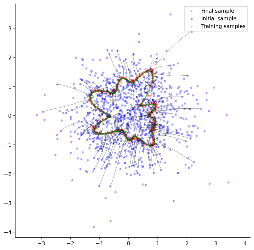
Figure 15: Example of learning to generate low-dimensional manifold with Song UNet-inspired MLP denoiser.

F.2 EDM Loss Function

We employ the loss function $\mathcal{L}_{\text{EDM}}$ introduced in the Elucidated Diffusion Model (EDM) paper (Karras et al., 2022), which is one specific weighting scheme for training diffusion models.

For each data point $\mathbf{x}\in\mathbb{R}^{d}$, the loss is computed as follows. The noise level for each data point is sampled from a log-normal distribution with hyperparameters $P_{\text{mean}}$ and $P_{\text{std}}$ (e.g., $P_{\text{mean}}=-1.2$ and $P_{\text{std}}=1.2$). Specifically, the noise level $\sigma$ is sampled via

$$\sigma=\exp\big{(}P_{\text{mean}}+P_{\text{std}}\,\epsilon\big{)},\quad\epsilon\sim\mathcal{N}(0,1).$$

The weighting function per noise scale is defined as:

$$w(\sigma)=\frac{\sigma^{2}+\sigma_{\text{data}}^{2}}{\left(\sigma\,\sigma_{\text{data}}\right)^{2}},$$

with hyperparameter $\sigma_{\text{data}}$ (e.g., $\sigma_{\text{data}}=0.5$). The noisy input $\mathbf{y}$ is created by the following,

$$\mathbf{y}=\mathbf{x}+\sigma\mathbf{n},\quad\mathbf{n}\sim\mathcal{N}\big{(}\mathbf{0},\,\mathbf{I}_{d}\big{)},$$

Let $D_{\theta}(\mathbf{y},\sigma,\text{labels})$ denote the output of the denoising network when given the noisy input $\mathbf{y}$, the noise level $\sigma$, and optional conditioning labels. The EDM loss per data point can be computed as:

$$\mathcal{L}(\mathbf{x})=w(\sigma)\,\|D_{\theta}(\mathbf{x}+\sigma\mathbf{n},\sigma,\text{labels})-\mathbf{x}\|^{2}.$$

Taking expectation over the data points and noise scales, the overall loss reads

$\displaystyle\mathcal{L}_{EDM}=\mathbb{E}_{\mathbf{x}\sim p_{data}}\mathbb{E}_{\mathbf{n}\sim\mathcal{N}(0,\mathbf{I}_{d})}\mathbb{E}_{\sigma}\Big{[}w(\sigma)\,\|D_{\theta}(\mathbf{x}+\sigma\mathbf{n},\sigma,\text{labels})-\mathbf{x}\|^{2}\Big{]}$ (46)

F.3 Experiment 1: Diffusion Learning of High-dimensional Gaussian Data

F.3.1 Data Generation and Covariance Specification

We consider learning a score-based generative model on synthetic data drawn from a high-dimensional Gaussian distribution of dimension $d=128$. Specifically, we first sample a vector of variances

$$\bm{\sigma}^{2}=\bigl{(}\sigma_{1}^{2},\sigma_{2}^{2},\dots,\sigma_{d}^{2}\bigr{)},$$

where each $\sigma_{i}^{2}$ is drawn from a log-normal distribution (implemented via torch.exp(torch.randn(…))). We then sort them in descending order and normalize these variances to have mean equals 1 to fix the overall scale. Denoting

$$\mathbf{D}=\mathrm{diag}\bigl{(}\sigma_{1}^{2},\ldots,\sigma_{d}^{2}\bigr{)},$$

we generate a random rotation matrix $\mathbf{R}\in\mathbb{R}^{d\times d}$ by performing a QR decomposition of a matrix of i.i.d. Gaussian entries. This allows us to construct the covariance

$$\bm{\Sigma}\;=\;\mathbf{R}\,\mathbf{D}\,\mathbf{R}^{\mathsf{T}}.$$

This rotation matrix $\mathbf{R}$ is the eigenbasis of the true covariance matrix. To obtain training samples $\{\mathbf{x}_{i}\}\subset\mathbb{R}^{d}$, we draw $\mathbf{x}_{i}$ from $\mathcal{N}\bigl{(}\mathbf{0},\bm{\Sigma}\bigr{)}$. In practice, we generate a total of $10{,}000$ samples and stack them as pnts. We compute the empirical covariance of the training set, $\bm{\Sigma}_{\text{emp}}=\mathrm{Cov}(\texttt{pnts}),$ and verify that it is close to the prescribed true covariance $\bm{\Sigma}$.

F.3.2 Network Architecture and Training Setup

We train a multi-layer perceptron (MLP) to approximate the noise conditional score function. The base network, implemented as

model=UNetBlockStyleMLP_backbone(ndim=d, nlayers=5, nhidden=256, time_embed_dim=256)

maps a data vector $\mathbf{x}\in\mathbb{R}^{d}$ and a time embedding $\tau$ to a vector of the same dimension $\mathbb{R}^{d}$. This backbone is then wrapped in an EDM-style preconditioner via:

$$\texttt{model\_precd}=\texttt{EDMPrecondWrapper}(\texttt{model},\sigma_{\text{data}}=0.5,\,\sigma_{\text{min}}=0.002,\,\sigma_{\text{max}}=80,\,\rho=7.0),$$

which standardizes and scales the input according to the EDM framework (Karras et al., 2022).

We use EDM loss with hyperparameters $\texttt{P\_mean}=-1.2$, $\texttt{P\_std}=1.2$, and $\sigma_{\text{data}}=0.5$. We train the model for $5000$ steps using mini-batches of size $1024$. The Adam optimizer is used with a learning rate $\texttt{lr}=10^{-4}$. Each training step processes a batch of data from pnts, adds noise with randomized noise scales, and backpropagates through the EDM loss. The loss values at each training steps are recorded.

F.3.3 Sampling and Trajectory Visualization

To visualize the sampling evolution, we define a callback function (sampling_callback_fn) that periodically draws new samples from a standard Gaussian, $\mathbf{z}\sim\mathcal{N}(\mathbf{0},\mathbf{I}_{d})$ and applies the Heun’s 2nd order deterministic sampler:

$\displaystyle\texttt{edm\_sampler}(\texttt{model},\mathbf{z},\texttt{num\_steps}=20,\,\sigma_{\text{min}}=0.002,\,\sigma_{\text{max}}=80,\,\rho=7).$

This returns the final samples x_out along with their intermediate trajectories x_traj in diffusion time. We store these trajectories in sample_store to track how sampling quality improves over epochs. After training is complete, we perform a final sampling run with $\texttt{num\_steps}=40$.

F.3.4 Covariance Evaluation in the True Eigenbasis

To measure how well the trained model captures the true covariance structure, we compute the sample covariance from the final generated samples, denoted $\widehat{\bm{\Sigma}}_{\text{sample}}$. We then project $\widehat{\bm{\Sigma}}_{\text{sample}}$ and the true $\bm{\Sigma}$ into the eigenbasis of $\bm{\Sigma}$. Specifically, letting $\mathbf{R}$ be the rotation used above, we compute

$$\mathbf{R}^{\mathsf{T}}\,\widehat{\bm{\Sigma}}_{\text{sample}}\,\mathbf{R}\quad\text{and}\quad\mathbf{R}^{\mathsf{T}}\,\bm{\Sigma}\,\mathbf{R}.$$

Since $\bm{\Sigma}=\mathbf{R}\,\mathbf{D}\,\mathbf{R}^{\mathsf{T}}$ is diagonal in that basis, we then compare the diagonal elements of $\mathbf{R}^{\mathsf{T}}\,\widehat{\bm{\Sigma}}_{\text{sample}}\,\mathbf{R}$ with $\mathrm{diag}(\mathbf{D})$. As training proceeds, we track the ratio $\mathrm{diag}(\mathbf{R}^{\mathsf{T}}\,\widehat{\bm{\Sigma}}_{\text{sample}}\,\mathbf{R})/\mathrm{diag}(\mathbf{D})$ to observe convergence toward 1 across the spectrum.

All intermediate results, including loss values and sampled trajectories, are stored to disk for later analysis.

F.4 Experiment 2: Diffusion Learning of MNIST — MLP

F.4.1 Data Preprocessing

For our second experiment, we apply the same EDM framework to a real image dataset. We select the MNIST dataset, which consists of handwritten digit images of size $28\times 28$. Each image is flattened to a 784-dimensional vector, yielding

$$\texttt{pnts}\in\mathbb{R}^{N\times 784},$$

where $N$ is the number of samples in MNIST (e.g. $60{,}000$ for the training set). We normalize these intensities from $[0,1]$ to $[-1,1]$ by applying the linear transformation

$$\mathbf{x}\;\mapsto\;\frac{\mathbf{x}-0.5}{0.5}.$$

The resulting data tensor pnts is then transferred to GPU memory for training, and we estimate its empirical covariance $\bm{\Sigma}_{\mathrm{emp}}=\mathrm{Cov}(\texttt{pnts})$ for reference.

F.4.2 Network Architecture and Training Setup

Since the MNIST dataset is higher dimensional than the synthetic data in the previous experiment, we use a deeper MLP network:

model $\displaystyle=\texttt{UNetBlockStyleMLP\_backbone}(\texttt{ndim}=784,\texttt{nlayers}=8,\texttt{nhidden}=1024,\texttt{time\_embed\_dim}=128).$

We again wrap this MLP in an EDM preconditioner:

$$\texttt{model\_precd}=\texttt{EDMPrecondWrapper}(\texttt{model},\,\sigma_{\text{data}}=0.5,\,\sigma_{\text{min}}=0.002,\,\sigma_{\text{max}}=80,\,\rho=7.0).$$

The model is trained using the EDMLoss described in the previous section, with parameters $\texttt{P\_mean}=-1.2$, $\texttt{P\_std}=1.2$, and $\sigma_{\text{data}}=0.5$. We set the training hyperparameters to $\texttt{lr}=10^{-4}$, $\texttt{n\_steps}=100000$, and $\texttt{batch\_size}=2048$.

F.4.3 Sampling and Analysis

As before, we define a callback function sampling_callback_fn that periodically draws i.i.d. Gaussian noise $\mathbf{z}\sim\mathcal{N}(\mathbf{0},\mathbf{I}_{784})$ and applies the EDM sampler to produce generated samples. These intermediate samples are stored in sample_store for later analysis.

In addition, we assess convergence of the mean of the generated samples by computing

$$\|\mathbb{E}[\texttt{x\_out}]\;-\;\mathbb{E}[\texttt{pnts}]\|^{2},$$

and we track how this mean-squared error evolves over training steps. We also examine the sample covariance $\widehat{\bm{\Sigma}}_{\text{sample}}$ of the final outputs, comparing its diagonal in a given eigenbasis to a target spectrum (e.g. the diagonal variances of the training data or a reference covariance).

All trajectories and intermediate statistics (mean_x_sample_traj, diag_cov_x_sample_true_eigenbasis_traj) are saved to disk for further inspection. In particular, we plot the difference between $\widehat{\bm{\Sigma}}_{\text{sample}}$ and $\bm{\Sigma}$ in an eigenbasis to illustrate whether the learned samples capture the underlying covariance structure of the MNIST training data.

F.5 Experiment 3: Diffusion learning of Image Datasets with EDM-style CNN UNet

We used model configuration similar to https://github.com/NVlabs/edm, but with simplified training code more similar to previous experiments.

For the MNIST dataset, we trained a UNet-based CNN (with four blocks, each containing one layer, no attention, and channel multipliers of 1, 2, 3, and 4) on MNIST for 50,000 steps using a batch size of 2,048, a learning rate of $10^{-4}$, 16 base model channels, and an evaluation sample size of 5,000.

For the CIFAR-10 dataset, we trained a UNet model (with three blocks, each containing one layer, wide channels of size 128, and attention at resolution 16) for 50,000 steps using a batch size of 512, a learning rate of $10^{-4}$, and an evaluation sample size of 2,000 (evaluated in batches of 1,024) with 20 sampling steps.

For the AFHQ (64 pixels) dataset, we trained a UNet model with four blocks (each containing one layer, wide channels of size 128, and attention at resolution 8) for 50,000 steps using a batch size of 256, a learning rate of $2\times 10^{-4}$, and an evaluation sample size of 1,000 (evaluated in batches of 512).

For the FFHQ (64 pixels) dataset, we used the same UNet architecture and training setup, with four blocks, wide channels of size 128, and attention at resolution 8, trained for 50,000 steps with a batch size of 256 and a learning rate of $2\times 10^{-4}$. Evaluation was conducted on 1,000 samples in batches of 512.

Training code can be found in attached supplementary material.