Reconsidering the calculation of the false vacuum decay rate at zero temperature
Abstract
In the calculation of the decay rate at finite temperature using the saddle point approximation, we identified some inconsistencies in the calculation of the decay rate at zero temperature. These inconsistencies may impact the explanation provided by Callan and Coleman. To address these inconsistencies, we recalculated the decay rate using the shifted-bounce solution and the shot solution.
I Introduction
In order to calculate the decay rate of the false vacuum state, Callan and Coleman put forward their method in [1, 2]. They used the relation between the decay rate of a metastable state and the corresponding imaginary part of its energy. They derived the imaginary part of the energy with the help of path integral formalism of the Euclidean transition amplitude. Then they obtained the final result after applying the saddle point approximation.
However, there are some ambiguities in the choice of the classical solutions and in the timing of taking the time interval to infinity. These ambiguities caused some problems, especially in the application of the collective coordinate method. Andreassen et al. tried to solve some problems in their paper [3] but there are more. We would like to describe related problems first and try to solve them using the shot solution presented in [3].
II Review of the decay rate at zero temperature
The central idea for deriving the decay rate is the following relation :
| (1) |
By taking the Euclidean time to infinity, the following relation can be obtained :
| (2) |
where is the energy of the state with the lowest energy. Since the decay process of a metastable state is considered, should be the energy of the metastable state with the smallest real part and the completeness relation used in Eq.(1) should be the completeness relation of the metastable states. The corresponding metastable state is called the false vacuum state. The decay rate corresponding to the metastable state is correlated with to the imaginary part of the complex energy as
| (3) |
Since the Euclidean transition amplitude can be expressed as the path integral formalism, the decay rate can be derived from the path integral formalism directly. Moreover, the calculation of the path integral can be performed by saddle point approximation.
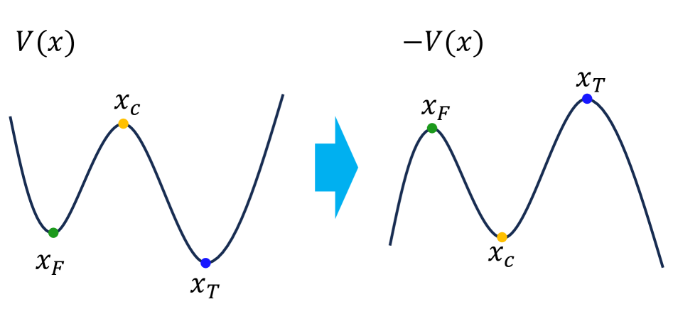
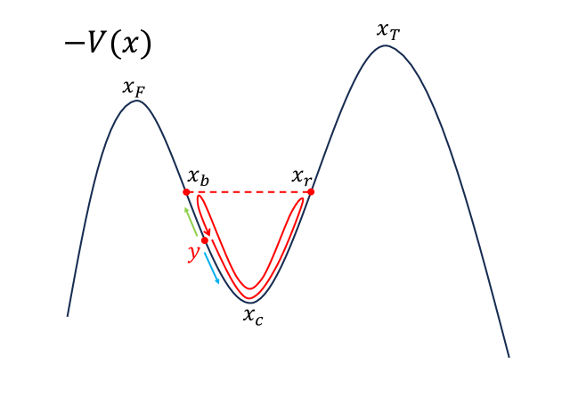
Consider a system with the potential shown in Figure.1. The decay process of the false vacuum state could occur in such a system. As the Euclidean transition amplitude is adopted, the potential in is reversed. Although the selection of the endpoints and is arbitrary, it is normally to choose them to be in most of the research. Therefore, a classical solution is required to satisfy
| (4) |
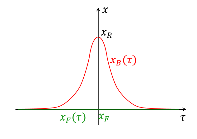
When is infinite, there are two classical solutions according to Callan and Coleman. One is called the false vacuum solution . The other is called the bounce .
After finding a classical solution , the path in the path integral can be expanded around as
| (5) |
Then the exponent becomes
| (6) |
at . The fluctuation can be expanded by the eigenfunctions of the fluctuation operator corresponding to the saddle point . satisfies the eigenequation
| (7) |
Furthermore, since is a classical solution, it should satisfy the same boundary condition as . As a result, and all s should satisfy the Dirichlet boundary conditions :
| (8) |
| (9) |
in order to be in consistency. Then the expansion around can be expressed as
| (10) |
And the contribution of to the original path integral can be expressed as
| (11) | ||||
| (12) | ||||
| (13) | ||||
| (14) |
For finite , the contribution from can be expressed as
| (15) |
where and is set to zero.
As for the bounce for infinite , its time derivative satisfies
| (16) |
and . Consequently, it corresponds to an eigenfunction with a zero eigenvalue. Moreover, has a node. Therefore, a negative eigenvalue also exists. As a result, the integral over (corresponding to the negative mode ) as well as (corresponding to the zero mode ) becomes infinite.
The infinity caused by was treated with analytic continuation. The negative eigenvalue indicates that the bounce solution is not a minimum of but a maximum along this special direction, which corresponds to , in the function space. Moreover, this direction was assumed to be attached to one steepest ascent direction from the false vacuum solution. By integrating over a series of paths parameterized by a real variable along the direction, the path integral can be written as
| (17) |
should satisfy and can be set to equal to at and at separately.
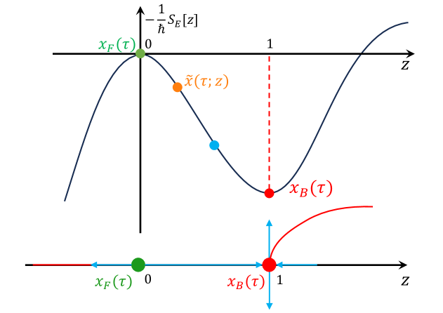
are assumed to reach minus infinity when becomes large enough. The divergence of will lead to the divergence of , which corresponds to the divergence of the integral over . Hence, in order to obtain a reasonable result, analytic continuation is required. Actually, the analytic continuation can be conducted by changing the integral contour from the real -axis to a new integral contour, which was distorted along the imaginary axis at . The new contour is the steepest descent contour passing through following the previous assumption. Along the new contour, the stationary point approximation becomes
| (18) |
The infinity caused by was treated with the so-called collective coordinate method. According to [2], the relation between the expansion coefficient of the zero eigenfunction and the time translations of the bounce solution is given by
| (19) |
since the small variation over can be expressed as
| (20) |
The relation indicates that the small variation over can be transformed into the small variation over . By use of and , the following relation can be obtained
| (21) |
The integration over is thought to be equivalent to the integrals over . As a result, it is concluded that there is no need to include the zero eigenvalue but to include a factor of since the integral over the center of the bounce has already been performed.
Combining the result above, the saddle point approximation can be expressed
| (22) | ||||
| (23) |
And the imaginary part of becomes
| (24) | ||||
| (25) |
where means excluding the zero eigenvalue. The decay rate at zero temperature then becomes
| (26) |
We should emphasize that the calculation of the ratio is carried out under the condition that the time interval is infinite. Parts of the classical solutions in were extracted in order to perform a possible calculation. The corresponding ratio related to these two partial classical solutions was calculated first and then was taken to infinity to obtain the final result. This method is different from the method starting from a finite time interval. And the here is chosen artificially and has nothing to do with the time interval .
III Reconsideration
There are at least two issues requiring further explanations in the previous derivation. The first concerns the appearance of an imaginary part in a Euclidean path integral. The second involves the timing of taking to infinity.
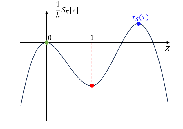
The first problem is somehow sophisticated. Part of the problem was already solved in [3]. Mathematically, the appearance of the imaginary part originates from the particular selection of the integral contour, or in other words, the selection of the saddle points. Actually, another classical solution called the shot solution exists according to [3]. The direction related to the negative mode of the bounce is assumed to be attached to the shot solution as well. Consequently, the shot solution will be another minimum and won’t reach minus infinity as becomes large. Therefore, the one dimensional integral Eq.(17) won’t diverge. In order to obtain the imaginary part, the integral contour should be chosen as the steepest descent contour passing through the false vacuum solution rather than the original real axis, which excludes the contribution from the shot solution and leads to the imaginary part. In other words, the imaginary part appears because of the selection of a special integral contour rather than a proper analytic continuation.
However, the reason for such a choice of contour was not fully explained in [3], especially for the Euclidean time formalism. We believe that the reason is related to the properties of the metastable states since such states with complex energies should be defined by particular boundary conditions which are different from the boundary conditions of the bound states. Such boundary conditions should show their influences apparently in the path integral, such as the choice of the integral contour. To solve the problem completely, we believe that some basic concepts such as the rigged Hilbert space (see [5])
which includes states with different boundary conditions such as Gamow vectors, should be considered since both states with complex energy and s used to generate the path integral formalism are vectors in the rigged Hilbert space. However, we won’t discuss the problem in this paper.
The second problem was confused at the beginning of the derivation of Callan and Coleman. Although they started their discussion from a finite time interval , they included the bounce solution with the endpoints at , which can only exist at an infinite time interval. If the contribution from the bounce solution is included while calculating the path integral by saddle point approximation, then all appearing in the intermediate process are merely symbols representing infinity rather than physical quantities with physical meanings. This problem is closely related to the validity of using the collective coordinate method.
Callan and Coleman used the collective coordinate method to deal with the zero mode existing in the fluctuation determinant of the bounce solution. The result of the zero mode should be , which is definitely infinite. It can’t be equal to if the integral range is finite. Therefore, it is impossible to use a finite physical integral
| (29) |
to represent an infinite integral unless the here is just a symbol representing infinity. In fact, as we discussed in our paper [6], the bounce solution with different endpoints also exists when the time interval is finite. Some may think that there is no zero mode of the fluctuation determinant of such bounce solution and only a quasi-zero mode at large time interval. Unfortunately, the fluctuation determinants of those bounce solutions also have an exact zero eigenvalue no matter what the time interval is since the initial velocities of these bounce solutions are always zero. As a result, their time derivatives serve as the eigenfunctions with zero eigenvalues, leading to divergence. Therefore, it can’t be expected that a smooth transition exists while the time interval changes from finite to infinite since the zero mode always exists.
According to Langer’s explanation in [7], shifted-bounces with different central values trace out a line in the function space. All points on the line have completely the same contributions. Consequently, the length of the line which is equal to was calculated instead of the zero mode. This explanation is similar to the explanation given in [3]. They tried to explain the inconsistencies appeared in using collective coordinate method from the point of view of the coordinate transformation. They changed the original integral over
| (30) |
to
| (31) |
However, both of their explanations are also insufficient. First, both explanations require that the original paths in the path integral should satisfy the periodic boundary conditions instead of the Dirichlet boundary condition. Otherwise, the boundary conditions of the original path can’t be satisfied for nonzero or large .
Furthermore, the equivalence between the two coordinate systems is suspicious. is a local coordinate system created around a saddle point while is a global coordinate axis in function space. They are definitely not equivalent for finite . Whether they become the same or not at infinite requires further proof. For simplicity, whether the relation Eq.(21) between and holds for all and requires further explanation.
IV Starting from finite time interval
In fact, if we admit the explanation for the first problem, we can avoid the second problem in calculating the transition amplitude. Although there is always a zero mode related to a bounce solution, it is actually not necessary to include a bounce solution. The shifted-bounce solution and the shot-F solution were used to calculate the free energy at finite temperature in our last paper [6]. They also exist when the time interval is finite and can be used to calculate the transition amplitude as well. Fortunately, the fluctuation operator of a shifted-bounce solution with nonzero initial velocity has no zero eigenvalue.
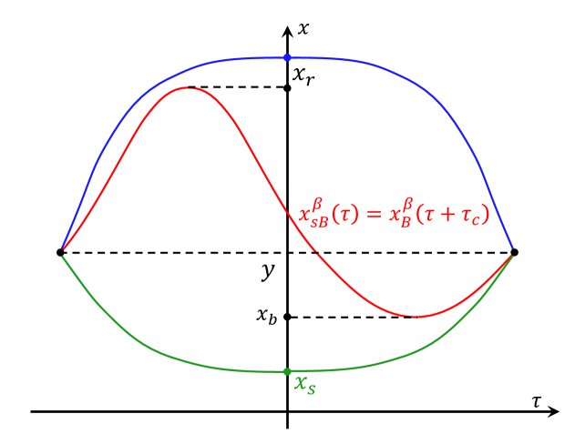
Consider the finite time interval , the endpoints of a bounce shift from to some other point . Since and can be chosen arbitrarily, they can be chosen to be , which is different from as shown in Figure.5.
| (32) |
Consequently, the related classical solutions are a shifted-bounce solution starting from and the corresponding shot-F solution . As long as the initial velocity of the shifted-bounce solution is not zero, no zero mode appears. We can calculate the transition amplitude from a “real” finite time interval and then take to infinity. All inside the limitation are finite.
Although there could be several classical solutions, since we take the integral contour to be the steepest descent contour passing through , only the contributions from the shifted-bounce solution and the shot-F solution are contained. As a result, the path integral can be expressed as
| (33) |
where the analytic continuation was performed and the contributions from other classical solutions were excluded in order to obtain an imaginary part111Actually, two shifted-bounce solutions with opposite initial velocities exist. Their contributions are the same. However, our main purpose focuses on the second issue mentioned in the previous section rather than providing a complete calculation. Therefore, we won’t discuss the choice for the classical solutions here. .
Then the imaginary part of the energy can be expressed as
| (34) | ||||
| (35) |
The ratio can be calculated as
| (36) |
where is the action of and is its energy. Denote the turning point of the shot-F solution as , then the ration can be expressed as
| (37) | ||||
| (38) |
When , . In order to obtain the final result, we need to find the limit relation between , and following the method used in [8].
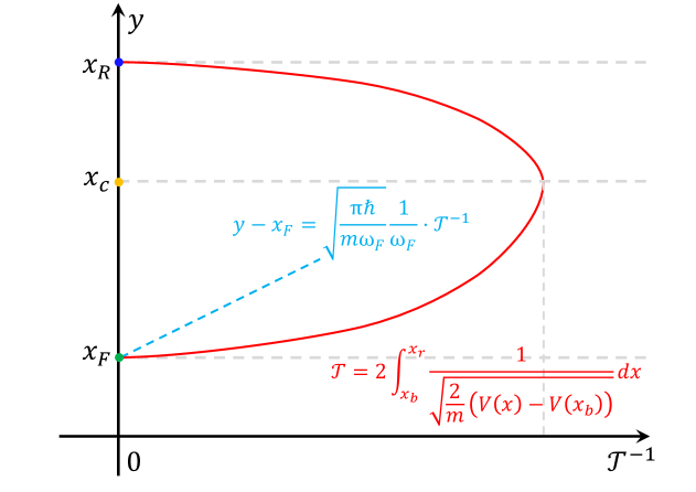
We start from the derivation of the limit of . Here, since is the time interval, it can be expressed as the integral :
| (39) |
The first integral can be re-expressed as
| (40) |
The additional integral can be conducted as
Consequently, the following relation can be obtained
| (41) |
Similarly, the relation between and can be obtained as
| (42) |
Then, we can get
| (43) |
As for , can be expressed as
| (44) |
by using the general formula for derivative of the implicit function. Therefore,
| (45) | ||||
| (46) | ||||
| (47) |
where we have used
| (48) |
The limit of can be calculated from the limit of since
| (49) |
And the limit of is already known from Eq.(41) as
| (50) |
As a result,
| (51) |
By combining the result obtained above, the final result of the limit of the ratio becomes
| (52) |
Therefore,
| (53) |
where we have set to make . The decay rate at zero temperature becomes
| (54) |
When , can be chosen to be in order to obtain a finite result. However, is selected artificially. The final result depends on the approaching behavior of and is not single. For comparison, we can re-express the exponent part as
| (55) |
where
| (56) |
Then, becomes
| (57) |
When is chosen to be , becomes infinite. Therefore, should reflect the zero mode related to the bounce.
In order to obtain a finite final result,
| (58) |
The choice is not unique. Furthermore, from Eq.(41) we can know that
| (59) |
Therefore, it can be speculated that
| (60) |
if was choose. Consequently, , which is expected.
The final result of Callan and Coleman can be obtained by choosing and to be
| (61) |
However, the constant of proportionality between and can be chosen arbitrarily (see Figure.7). Consequently, the result can be any value. This appears like the ratio between two irrelevant infinite values. We believe that this fact indicates the relation between the zero mode of the bounce solution and the infinite time interval.
V Summary
In this paper we discussed two issues in the calculation of the decay rate at zero temperature. We believe that the first problem related to the appearance of the imaginary part can be solved once the states in the rigged Hilbert space are taken into consideration. As for the second problem, which is related to the timing to take the time interval to infinity and is the main topic in our paper, we have recalculated the transition amplitude by using saddle point approximation at finite time interval. We have utilized the shot-F solution and the shifted-bounce solution instead of the bounce solution. Since no zero eigenvalue appears, there is no need to introduce the collective coordinate method and the equivalence problem between the two infinite values is avoided. When taking the time interval to infinity, we can obtain a finite result if we choose the proper classical solutions. However, we find that the final result depends on how the limit is taken and is not unique. As we mentioned in Section.III, the validity of the collective coordinate method used to deal with the zero mode as well as the equivalence between the integral over and should be discussed in more detail.
VI Appendix
VI.1 The Calculation of Functional Determinants
The problem of deriving a functional determinant can be transformed to solving the eigenequation under the corresponding initial conditions. We here simply present the result (see [9, 10, 11, 12, 13, 14, 15, 16, 17] for more details).
The ratio of two functional determinant defined over by Dirichlet boundary conditions can be expressed as
| (62) |
where is the solution to the following equation
| (63) |
and satisfies the following initial conditions
Now, consider the fluctuation determinant of a classical solution . Since is a classical solution, it must obey the equation of motion
| (64) |
We can take the partial derivative of the equation of motion with respect to a parameter which is explicitly contained in but not in on both side. Then we get
| (65) |
So is just a solution to Eq.(63). But pay attention, we can’t assert that is an eigenfunction since may not satisfy the boundary condition.
When is chosen to be , becomes , which is the velocity of the classical solution . If it is noticed that classical solutions exist for every energy in a given range, then it is natural to realize that also depends on the energy . Therefore, can be chosen to be as well (see [8]). Denote , then is another solution.
Before focusing on the function that meets the initial conditions, we would like to discuss the properties of in more detail.
First, the linear independence of and can be proven immediately. Since is the classical solution in Euclidean time, its energy is conserved over Euclidean time :
| (66) |
Taking the derivative of Eq.(64) over energy gives
| (67) |
Using the equation of motion and the commutative property of partial derivatives, the following relation can be derived:
| (68) |
Therefore, the Wronskian of and is a non-zero constant, which indicates that and are linearly independent.
Next, it must be emphasized that the periodicity of is different from that of . Even if is the periodic function with period of ( doesn’t need to be equal to ), may not be periodic since the period could also depend on the energy of classical orbit. As a result, considering , the following relation holds
| (69) |
Finally, the parity of is the same as that of . If is an odd or even function with regard to the Euclidean time , then will exhibit the same parity.
Since two independent solutions have been found, can be constructed as
| (70) |
-
1.
For a shot solution :
(71) becomes
(72) (73) (74) -
2.
For the shifted-bounce solution :
(75) becomes
(76) (77) (78)
Therefore, the following relation can be obtained.
| (79) |
Acknowledgements.
The authors is grateful to Prof. Koji Harada and Prof. Shuichiro Tao for valuable discussions. This work is supported by Kyushu University Leading Human Resources Development Fellowship Program (Quantum Science Area).References
- [1] Sidney R. Coleman. The fate of the false vacuum. i. semiclassical theory. Phys. Rev. D, 15:2929–2936, May 1977.
- [2] Curtis G. Callan, Sidney Coleman. Fate of the false vacuum. ii. first quantum corrections. Physical Review D, 16(6):1762–1768, September 1977.
- [3] Anders Andreassen, David Farhi, William Frost, Matthew D. Schwartz. Precision decay rate calculations in quantum field theory. Physical Review D, 95(8):085011, April 2017.
- [4] Sidney Coleman. Aspects of Symmetry: Selected Erice Lectures. Cambridge University Press, 1985.
- [5] Arno Böhm, M. Loewe. Quantum Mechanics: Foundations and Applications. Springer-Verlag, 1993.
- [6] Koji Harada, Shuichiro Tao, Qiang Yin. Saddle-point approximation to the false-vacuum decay at finite temperature in 1d quantum mechanics. Progress of Theoretical and Experimental Physics, 2025(1):013A01, January 2025.
- [7] J. S Langer. Theory of the condensation point. Annals of Physics, 41(1):108–157, January 1967.
- [8] Marcos Marino. Instantons and Large N: An Introduction to Non-Perturbative Methods in Quantum Field Theory. Cambridge University Press, Cambridge, 2015.
- [9] I. M. Gel’fand, A. M. Yaglom. Integration in functional spaces and its applications in quantum physics. Journal of Mathematical Physics, 1(1):48–69, January 1960.
- [10] A. J. McKane, M. B. Tarlie. Regularization of functional determinants using boundary perturbations. Journal of Physics A: Mathematical and General, 28(23):6931, December 1995.
- [11] Klaus Kirsten, Alan McKane. Functional determinants by contour integration methods. Annals of Physics, 308(2):502–527, December 2003.
- [12] Klaus Kirsten, Alan J. McKane. Functional determinants for general sturm-liouville problems. Journal of Physics A: Mathematical and General, 37(16):4649–4670, April 2004.
- [13] Gerald V. Dunne, Klaus Kirsten. Functional determinants for radial operators. Journal of Physics A: Mathematical and General, 39(38):11915–11928, September 2006.
- [14] Gerald V. Dunne. Functional determinants in quantum field theory. Journal of Physics A: Mathematical and Theoretical, 41(30):304006, August 2008.
- [15] Klaus Kirsten. Functional determinants in higher dimensions using contour integrals. arXiv:1005.2595 [hep-th, physics:math-ph, physics:quant-ph], May 2010.
- [16] G. M. Falco, Andrei A. Fedorenko, Ilya A. Gruzberg. On functional determinants of matrix differential operators with multiple zero modes. Journal of Physics A: Mathematical and Theoretical, 50(48):485201, November 2017.
- [17] A. Ossipov. Gelfand-yaglom formula for functional determinants in higher dimensions. Journal of Physics A: Mathematical and Theoretical, 51(49):495201, December 2018.