Weighted balanced truncation method for approximating kernel functions by exponentials

Abstract

Kernel approximation with exponentials is useful in many problems with convolution quadrature and particle interactions such as integral-differential equations, molecular dynamics and machine learning. This paper proposes a weighted balanced truncation to construct an optimal model reduction method for compressing the number of exponentials in the sum-of-exponentials approximation of kernel functions. This method shows great promise in approximating long-range kernels, achieving over $4$ digits of accuracy improvement for the Ewald-splitting and inverse power kernels in comparison with the classical balanced truncation. Numerical results demonstrate its excellent performance and attractive features for practical applications.

I Introduction

Approximating univariate kernel functions by exponentials is a useful technique for constructing fast algorithms of problems with convolution quadrature and particle interactions. The design of the so-called sum-of-exponentials (SOE) approximation has attracted broad interest in areas such as fast convolution [1, 2], electrostatic calculation [3], molecular dynamics simulation [4, 5, 6], dynamics of magnetic nanoparticle [7], dynamics of non-Markovian systems [8], and DNA melting curves [9]. Particularly, the kernel-independent SOE methods, including the black-box algorithm [2] and de la Vallée-Poussin model reduction method [10], have been proposed, providing efficient tools for kernel summation problems.

The number of exponentials determines the processing efficiency of subsequent fast algorithms. The Laplace transform of the SOE results in a sum of poles (SOP) which has also a number of applications such as electromagnetics [11]. In control theory, the SOP is the transfer function of linear dynamical systems, which can be compressed by building on the balanced truncation method and the square root method [12, 13]. The model reduction (MR) technique of the balanced truncation plays a crucial role in further decreasing the number of exponentials, exhibiting a significantly faster convergence rate compared to other approaches such as the classical Prony’s method [14]. However, the long-range nature of the kernel functions leads to the difficulty of efficient compression, and a direct use of the classical MR remains a big number of exponentials. Other methods such as the damping Newton method [15, 3] and Remez algorithm [16, 17] are also developed for optimal SOE approximation, mostly for the $1/r$ Coulomb kernel.

In this paper, we propose a weighted balanced truncation (WBT) method for optimizing the MR process, which facilitates more efficient and convenient reduction over a given interval and achieves faster convergence rates. By introducing a weight function into the balanced truncation process, the WBT enhances the uniformity of approximation error distribution on the provided interval. Given the same number of terms, the WBT method, as a novel kernel-independent SOE approximation technique, demonstrates several orders of magnitude improvement for general long-range kernels compared to the classical MR technique [10]. It exhibits nearly optimal performance for the Coulomb kernel with respect to the former works [3, 17], which further demonstrates its great application potential in scientific computing and physical problems.

The WBT is a generalization of the classical balanced truncation method, which is a simple and efficient approach to construct an improved model reduction scheme for many problems such as high-dimensional dynamical systems [18, 19, 20, 21] and multiscale modelling [22, 23].

II Method

Given an error criteria $\epsilon$ and an $N$-term SOE series, the goal of this paper is to compress the number of exponentials such that $P$ is minimized under the error level:

$$\left|\sum\limits_{j=1}^{N}\omega_{j}e^{-s_{j}r}-\sum\limits_{j=1}^{P}\tilde{\omega}_{j}e^{-\tilde{s}_{j}r}\right|<\epsilon,$$ (II.1)

for $r\in[0,M]$. In general, a preliminary and high-accurate SOE approximation of an interested kernel can be obtained by some kernel-independent techniques [2, 10]. Minimizing the number of exponentials in a given interval will significantly improve the simulation efficiency. The minimum problem can be calculated by the balanced truncation method, following the work of [12, 13]. Here, we introduce a novel weighted balanced truncation method, which will promote the performance of compression, leading to an improved model reduction method.

To present the WBT idea, one starts from the Laplace transform of the $N$-term SOE series and represents the resultant sum-of-poles (SOP) by a matrix form,

$$\mathcal{L}\left[\sum_{j=1}^{N}\omega_{j}e^{-s_{j}r}\right]=\sum_{j=1}^{N}\frac{\omega_{j}}{z+s_{j}}=\bm{c}(z\bm{I}-\bm{A})^{-1}\bm{b},$$ (II.2)

where $\bm{A}=-\mathrm{diag}\{s_{1},\cdots,s_{N}\}$ is an $N\times N$ diagonal matrix, $\bm{b}=(\sqrt{|\omega_{1}|},\cdots,\sqrt{|\omega_{N}|})^{T}$ and $\bm{c}=(sgn(\omega_{1})\sqrt{|\omega_{1}|},\cdots,sgn(|\omega_{N}|)\sqrt{|\omega_{N}}|)$ are column and row vectors of dimension $N$, respectively. The sign function $sgn(x)=x/|x|$ for nonzero $x$ and $sgn(0)=0$.

The matrix form of the SOP can be considered as the transfer function of the following linear dynamical system

$$\left\{\begin{array}[]{l}\dot{\bm{x}}=\bm{A}\bm{x}(t)+\bm{b}w(-t)u(t),\\ y(t)=\bm{c}w(t)\bm{x}(t),\end{array}\right.$$ (II.3)

where $u(t)$ and $y(t)$ are the input and output of this system, respectively, and $w(t)>0$ is a weight function. If $\hat{u}(z)$ and $\hat{y}(z)$ are Laplace transforms of the weighted input $w(-t)u(t)$ and output $y(t)/w(t)$, then they can be connected by the transfer function

$$\hat{y}(z)=\bm{c}(z\bm{I}-\bm{A})^{-1}\bm{b}\hat{u}(z).$$ (II.4)

Here we introduce the weight function $w(t)$ in order to construct an optimal model reduction. In the case of the Heaviside function, i.e., $w(t)=H(t)$ with $H(t)=1$ for $t\geq 0$ and $0$ otherwise, it is applied in constructing the original balanced truncation method, and has been widely discussed [12, 13].

By the transfer function, the reduction on the SOE series can be performed by the explicit solution of the linear dynamical system (II.3),

$$y(t)=\int_{-\infty}^{t}\bm{c}w(t)e^{\bm{A}(t-\tau)}\bm{b}w(-\tau)u(\tau)\mathrm{d}\tau.$$ (II.5)

In this work, one assumes that the weight function $w(t)$ is compactly supported on the interval $[0,T]$. Define the solution operator $\mathcal{H}$ such that $y(t)=\mathcal{H}u(t)$, and $\mathcal{H}^{*}$ being the conjugate operator. Due to the compactness of the weight function, one can express them by,

$$\left\{\begin{aligned} \mathcal{H}u(t)&=\int_{-\infty}^{+\infty}\bm{c}w(t)e^{\bm{A}(t-\tau)}\bm{b}w(-\tau)u(\tau)\mathrm{d}\tau\\ \mathcal{H}^{*}y(t)&=\int_{-\infty}^{+\infty}\bm{b}^{*}w^{*}(-t)e^{\bm{A}^{*}(\tau-t)}\bm{c}w^{*}(\tau)y(\tau)\mathrm{d}\tau.\end{aligned}\right.$$ (II.6)

The key to reduce the linear system lies in calculating the singular values $\{\sigma_{i}\}$ of operator $\mathcal{H}$. Let these singular values be in an descending order with corresponding eigenfunctions $\{u_{i}(t)\}$, i.e., one has $\mathcal{H}^{*}\mathcal{H}u_{i}(t)=\sigma_{i}^{2}u_{i}(t)$. Indeed, using Eq. (II.6), one obtains the eigenfunction,

$$u_{i}(t)=\frac{1}{\sigma_{i}^{2}}\bm{b}^{*}w^{*}(-t)e^{-\bm{A}^{*}t}\bm{Q}\bm{v},$$ (II.7)

with

$$\bm{Q} =\int_{-\infty}^{+\infty}e^{\bm{A}^{*}t}\bm{c}^{*}\bm{c}e^{\bm{A}t}w(t)w^{*}(t)\mathrm{d}t,$$ (II.8)

$$\bm{v} =\int_{-\infty}^{+\infty}e^{-\bm{A}\tau}\bm{b}w(-\tau)u_{i}(\tau)\mathrm{d}\tau.$$

Substituting Eq. (II.7) into the expression of $\bm{v}$ in Eq. (II.8), one has $\sigma_{i}^{2}\bm{v}=\bm{P}\bm{Q}\bm{v}$ with

$$\bm{P}=\int_{-\infty}^{+\infty}e^{\bm{A}t}\bm{b}\bm{b}^{*}e^{\bm{A}^{*}t}w(t)w^{*}(t)\mathrm{d}t.$$ (II.9)

Such $\bm{P}$ and $\bm{Q}$ are usually called Gramians in control theory [12]. One finds that $\sigma_{i}^{2}$ is eigenvalue of matrix $\bm{P}\bm{Q}$, i.e. $\sigma_{i}=\sqrt{\lambda_{i}(\bm{P}\bm{Q})}$, where $\lambda_{i}(\bm{P}\bm{Q})$ denotes the $i$-th eigenvalue. One calculates the expressions in Eqs. (II.8) and (II.9) to obtain the entries of matrix $\bm{P}$ and $\bm{Q}$,

$$\left\{\begin{array}[]{l}\bm{P}_{ij}=\sqrt{|\omega_{i}\omega_{j}|}I_{w}(s_{i},\overline{s}_{j})\\ \\ \bm{Q}_{ij}=sgn(\overline{\omega}_{i})sgn(\omega_{j})\sqrt{|\omega_{i}\omega_{j}|}I_{w}(\overline{s}_{i},s_{j}),\end{array}\right.$$ (II.10)

where the weighted integral $I_{w}$ is defined by

$$I_{w}(x,y):=\int_{-\infty}^{+\infty}e^{-(x+y)t}w(t)w^{*}(t)\mathrm{d}t.$$ (II.11)

The WBT procedure starts by computing the Gramians $\bm{P}$ and $\bm{Q}$ using Eq. (II.10). One then performs Cholesky factorizations $\bm{P}=\bm{S}\bm{S}^{*}$ and $\bm{Q}=\bm{L}\bm{L}^{*}$, followed by the singular value decomposition $\bm{S}^{*}\bm{L}=\bm{U}\bm{\Sigma}\bm{V}^{*}$ with $\bm{\Sigma}=\mathrm{diag}\{\sigma_{1},\sigma_{2},\dots,\sigma_{N}\}$. Let $\bm{R}=\bm{S}\bm{U}\bm{\Sigma}^{-1/2}$, one takes the linear transform $\bm{\widetilde{A}}=\bm{R}^{-1}\bm{A}\bm{R}$, $\widetilde{\bm{b}}=\bm{R}\bm{b}$ and $\widetilde{\bm{c}}=\bm{c}\bm{R}^{-1}$, toghther with the congruent transformations $\bm{\widetilde{P}}=\bm{R}^{-1}\bm{P}(\bm{R}^{-1})^{*}$ and $\bm{\widetilde{Q}}=\bm{R}^{*}\bm{Q}\bm{R}$. These two matrices are now diagonal, $\bm{\widetilde{P}}=\bm{\widetilde{Q}}=\bm{\Sigma}.$ The singular values are arranged in descending order, enabling the extraction of the principal information here. Specifically, the $P\times P$ principal block $\bm{\widetilde{A}}_{P}$ of $\bm{\widetilde{A}}$ is extracted, and the first $P$ dimensions of the vectors $\bm{\widetilde{b}}$ and $\bm{\widetilde{c}}$ are selected to form new vectors $\widetilde{\bm{b}}_{P}$ and $\widetilde{\bm{c}}_{P}$. Then through the transform by transition matrix $\bm{X}$ making $\bm{\Lambda}=\bm{X}^{-1}\widetilde{\bm{A}}_{P}\bm{X}$ diagonal, a new linear system $(\bm{\Lambda},\hat{\bm{b}},\hat{\bm{c}})$ is constructed with $\hat{\bm{b}}=\bm{X}^{-1}\widetilde{\bm{b}}_{P}$ and $\hat{\bm{c}}=\widetilde{\bm{c}}_{P}\bm{X}$. One can perform reduction operations and obtain a refined $P$-term SOE approximation of the original $N$-term SOE from the reduced linear system after the inverse Laplace transformation.

The Gramians $\bm{P}$ and $\bm{Q}$ in Eqs. (II.8) and (II.9) are positive definite, and thus their Cholesky factorizations exist. This leads to the validity of the WBT. The complete algorithm of the WBT method is summarized in Algorithm 1.

1:For a given SOE with weight function $w(r)$ with $N$ exponentials, initialize the matrix and vectors $\bm{A},\bm{b}$ and $\bm{c}$ by Eq. (II.3). Set the constant $P<N$. The algorithm is composed of the following steps.

2:Compute the Gramians $\bm{P}$ and $\bm{Q}$ by Eq. (II.10), perform Cholesky factorization for these two matrices such that $\bm{P}=\bm{S}\bm{S}^{*}$ and $\bm{Q}=\bm{L}\bm{L}^{*}$, and execute SVD factorization $\bm{S}^{*}\bm{L}=\bm{U}\bm{\Sigma}\bm{V}^{*}$ where the diagonal matrix $\bm{\Sigma}=\mathrm{diag}\{\sigma_{1},\sigma_{2},\cdots,\sigma_{N}\}$.

3:Set the transition matrix $\bm{R}=\bm{S}\bm{U}\bm{\Sigma}^{-1/2}$ to obtain the transformed linear dynamical system $\widetilde{\bm{A}}=\bm{R}^{-1}\widetilde{\bm{A}}\bm{R},\widetilde{\bm{b}}=\bm{R}\widetilde{\bm{b}}$ and $\widetilde{\bm{c}}=\widetilde{\bm{c}}\bm{R}^{-1}$. Consequently, the resultant Gramians are diagonal, namely, $\widetilde{\bm{P}}=\widetilde{\bm{Q}}=\bm{\Sigma}$.

4:Extract the $P\times P$ principal block of $\widetilde{\bm{A}}$, the first $P$ identities of $\widetilde{\bm{b}}$ and $\widetilde{\bm{c}}$, yielding $\widetilde{\bm{A}}_{P}$, $\widetilde{\bm{b}}_{P}$ and $\widetilde{\bm{c}}_{P}$. Perform eigenvalue decomposition $\widetilde{\bm{A}}_{P}=\bm{X}\bm{\Lambda}\bm{X}^{-1}$ such that $\bm{\Lambda}=\mathrm{diag}\{\tilde{s}_{1},\cdots,\tilde{s}_{P}\}$. Here, $\tilde{s}_{i}$ is the exponent of the $i$th exponentials in the reduced SOE. Compute $\hat{\bm{b}}=\bm{X}^{-1}\widetilde{\bm{b}}_{P}$ and $\hat{\bm{c}}=\widetilde{\bm{c}}_{P}\bm{X}$. The weights are then calculated by $\tilde{\omega}_{i}=\hat{\bm{b}}_{i}\hat{\bm{c}}_{i},\,i=1,2,\cdots,P$.

Algorithm 1 The weighted balanced truncation method

It worths to mention that the time-limited balanced truncation (TLBT) method [24, 25, 26] is a special case of the WBT. The TLBT sets $w(t)=H(t)-H(t-T)$, accounting for the interval effect on model reduction, and has been applied to large scale systems [27], discrete-time systems [28], semi-Markovian jump systems based on generalized Gramians [29] and data assimilation [30]. The WBT can be considered as a generalization of the TLBT, potentially providing higher accuracy for the model reduction. Thus, the WBT shall be also useful in many model order reduction problems besides the SOE approximation. One directional use is to construct sum-of-Gaussians (SOG) approximation to interacting and convolution kernels to design fast algorithms for particle systems [31, 32, 2, 33, 34] and nonlocal problems in high-dimensional spaces [35, 36]. The optimal truncation $T$ and weight function $w(r)$ for specific problems require a systematic study and remain open issues.

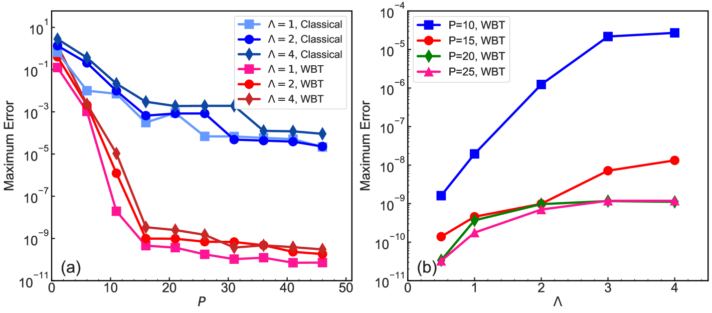
Figure 1: Maximum errors of SOE approximations of the Ewald splitting kernel on $[0,10]$. (a) Maximum errors with respect to the reduction term $P$, computed using both the classical MR and the WBT; (b) Maximum errors with respect to the kernel parameter $\Lambda$, computed using the WBT.

III Results

We perform numerical results to demonstrate the performance of the proposed WBT method. Three benchmark examples are studied, including a smooth Ewald splitting kernel, the Coulomb kernel for different weights and the inverse power kernels, in comparison with results of the model reduction method with the classical balanced truncation (denoted by ‘classical’ in legends). Unless otherwise stated, all weight functions in the following results are truncated within their target intervals.

III.1 Smooth Ewald-splitting kernel

Consider the Ewald splitting kernel $\mathrm{erf}(\Lambda r)/r$ with $\mathrm{erf}(\cdot)$ denoting the error function and $\Lambda$ being a positive constant. This kernel is often studied for Coulomb systems, resulted by the Ewald splitting of $1/r$ kernel. It is a typical smooth kernel with long-range nature. Consider the approximation on interval $[0,10]$ and parameter $\Lambda=1,2$ and $4$. One introduces the VP-sum method [10] for an $N$-term accurate SOE approximation of the kernel function. With $N=300$, the initial SOE series achieves the maximum errors at the level of $10^{-10}$. As a kernel-independent approximation method, the VP-sum involves extensive numerical integration and high-order polynomial parameter estimation. Achieving machine precision requires more expansion terms, which increases computational cost and leads to numerical instability. The accuracy of $10^{-10}$ ensures the stability of the VP and facilitates further comparison.

For the convenience of usage, we provide a comprehensive MATLAB software, VP-WBT, powered by the Multiprecision Computing Toolbox [37]. This software is capable of performing high-precision SOE or SOG approximations for general kernels and customized weight functions. The following numerical results can be simply reproduced through the visual interface of the software.

In Fig. 1(a), we present the maximum errors of the WBT method and the classical MR results for the three $\Lambda$ with the increase of $P$. In the calculations, one sets the weight function $w(r)=1$ and truncation parameter $T=M=10$. One can observe the exponential decay of the error with $P$, rapidly approaching an error level under $10^{-9}$ with about 16 exponentials for all $\Lambda=1$ and $2$. It is noted that, a larger $\Lambda$ corresponds to a slower decay of the kernel, resulting in a slightly larger error. In the case of $P=16$ and $\Lambda=4$, the error is $3.41\times 10^{-9}$. In comparison, the classical MR method is at the level of $10^{-3}$ accuracy for $P=16$. For larger $P$, the WBT error remains the same level as the original $300$-term SOE series. These results clearly demonstrate the rapid convergence of the WBT method in approximating smooth kernels.

Under the identical settings, we also consider the approximation effect with respect to increasing Ewald splitting kernel parameters $\Lambda=0.5,1,2,3$ and $4$ for fixed $P$. Fig. 1(b) shows that as $\Lambda$ increases, the maximum error of the WBT method initially grows rapidly and then tends to stabilize. The result reveals that for Ewald-splitting kernels with larger $\Lambda$, which exhibit stronger near-origin singularity and long-range behavior, the WBT method can provide an efficient and stable approximation. This further demonstrates the broad applicability of our proposed WBT method to kernel functions with different hard-to-handle properties.

III.2 Coulomb kernel with different weights

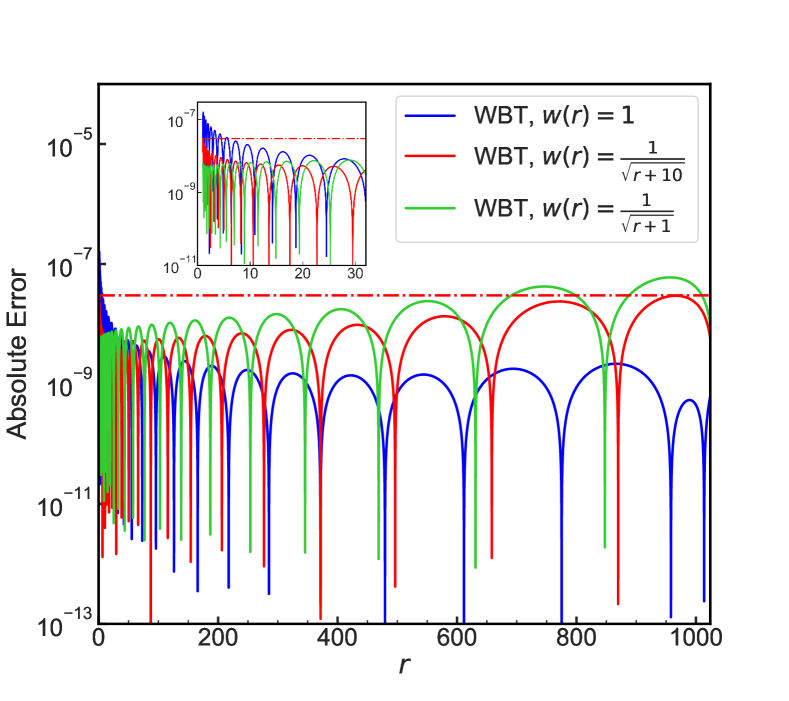
Figure 2: The error distribution of the WBT for the Coulomb kernel with different weight functions. The approximation interval is $[1,1024]$ with $P=15$ reduced SOE terms. The red dashed horizonal line represents the maximum error ($3.0\times 10^{-8}$) of $w(t)=1/\sqrt{r+10}$ situation.

To investigate the influence of the weight function $w(t)$ in WBT, we consider the Coulomb kernel $1/r$ on $[1,1024]$ using three different weight functions $w(r)\equiv 1,1/\sqrt{r+1}$ and $1/\sqrt{r+10}$. The preliminary SOE of the Coulomb kernel is derived from the bilateral series approximation (BSA) [38, 39],

$$r^{-\alpha}\approx\frac{\log(b)}{\Gamma(\alpha)}\sum_{\ell=-\infty}^{+\infty}b^{\alpha\ell}e^{-b^{\ell}r},$$ (III.1)

where $\Gamma(\cdot)$ denotes the gamma function and $\alpha=1$ for the Coulomb kernel. The base parameter $b>1$ determines the accuracy of the BSA approximation, which converges rapidly as $b$ asymptotically approaches 1. Here one sets $b=1.1$ and the truncation parameter $T=512$. Fig. 2 presents the error distributions with $P=15$ for the three weights. One can observe that the error distribution for $w(r)=1$ is quite nonuniform. The error near $r=1$ is much larger than the region away from the origin. The error distributions with the other two weight functions behave much better. Among the three weights, the maximum error of the $w(r)=1/\sqrt{r+10}$ case is smallest, which is $3.0\times 10^{-8}$. For comparison, the maximum errors for the $w(r)\equiv 1$ and $1/\sqrt{r+1}$ cases are $1.9\times 10^{-7}$ and $6.0\times 10^{-8}$, respectively. The results demonstrate that the WBT can be very efficient when an appropriate weight function is employed.

III.3 Convergence of inverse power kernel

We consider inverse power kernel $f(r)=r^{-\alpha}$ with the BSA in Eq. (III.1) for the preliminary SOE approximation of $N=500$ on the interval $[1,1024]$ with $b=1.1$, which is at the machine precision. In the WBT, one selects $T=512$ and weight function $w(r)=1/\sqrt{r+10}$.

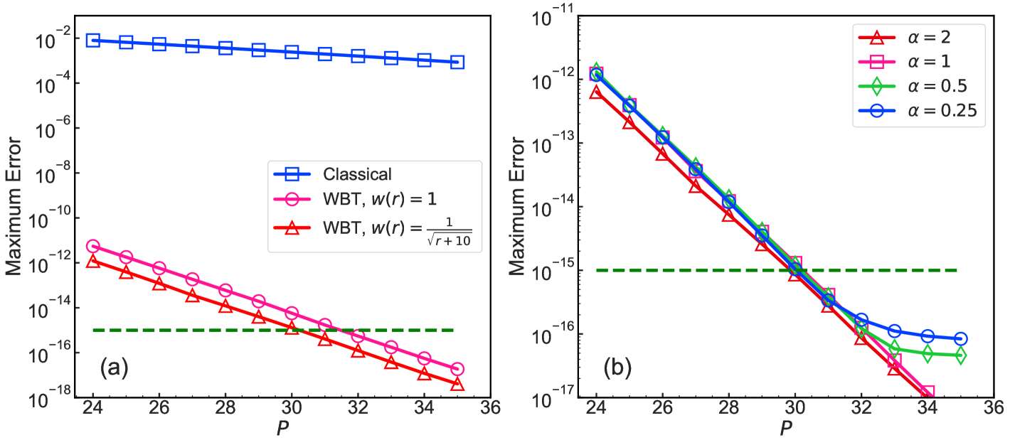
Figure 3: Maximum errors of SOE approximations of power function kernel on $[1,1024]$ with respect to the reduction term $P$. (a) Coulomb kernel reduced by different model reduction techniques, (b) Singular power functions with different $\alpha$ reduced by WBT. The green dashed line represents the precision of $1.0\times 10^{-15}$.

We first examine the accuracy of the Coulomb kernel for the $\alpha=1$ case with varying $P$, and the results are present in Fig. 3(a). One observes that the classical MR method exhibits a slow convergence rate in reducing the BSA sequence, while the WBT demonstrates remarkably fast convergence with over $9$ digits of accuracy improvement for $P>24$, achieving the maximum error of $7\times 10^{-16}$ with $31$ terms. This significant improvement arises because the WBT avoids the influence of long-range contributions outside the interval, which could otherwise affect the reduction and extraction of principal information. In contrast, the classical MR method has limitations in this regard, leading to slow convergence. Compared to the VP-sum with equidistant bandwidths in Section III.1, this advantage of the WBT method is particularly evident when applied to the BSA with exponentially distributed bandwidths. Indeed, the approximation provided by WBT reaches the same accuracy as the well-known results reported by Gimbutas et al. [3] Hackbusch et al. [17], which introduced complex optimization techniques such as the damping Newton and Remez algorithm. It is noted that the WBT method avoids these complex techniques, making it competitive for more general kernels for broad applications. Moreover, it is also possible to achieve even better results by leveraging optimization techniques with detailed analysis of the weight function $w(t)$ and truncation parameter $T$.

For different inverse power kernels, Fig. 3(b) presents the convergence results with $\alpha=0.25,0.5,1$ and $2$. With the same approximation interval and accuracy requirements, the WBT method delivers highly consistent approximation performance with the case of $\alpha=1$. It achieves the precision of $1.0\times 10^{-15}$ for all the cases for $P=31$, demonstrating that the WBT can effectively achieve the nearly optimal SOE approximation for various forms of error decay tails.

IV Conclusion

In summary, we propose a novel weighted balanced truncation method for approximating general kernel functions with exponentials. The WBT method incorporates a weight function into the balanced truncation method, resulting in a more accurate approximating precision across the target interval. Numerical examples clearly demonstrate that the WBT method achieves significant improvement in accuracy compared to classical model reduction method. As a general approximation technique for kernel functions, it provides nearly optimal approximation results for important kernels like the Coulomb interaction. Meanwhile, the WBT method maintains stable performance when handling functions with complex properties, leading to a broad application prospect in physics and scientific computing.

Besides treated as a kernel-independent approximation technique, WBT can also be regarded as an improved model order reduction method with even broader applicability. Future work will focus on designing efficient applications of the WBT method in cutting-edge fields, such as machine learning and materials computation.

Conflict of interest

The authors declare that they have no conflict of interest.

Data Availability Statement

The software package generating the data in this work is developed based on the MATLAB and the Multiprecision Computing Toolbox. The source code is available at https://github.com/linyuanshen114/VP-WBT.

References

- Lubich and Schädle [2002] C. Lubich and A. Schädle, SIAM Journal on Scientific Computing 24, 161 (2002).
- Greengard et al. [2018] L. Greengard, S. Jiang, and Y. Zhang, SIAM Journal on Scientific Computing 40, A3733 (2018).
- Gimbutas et al. [2020] Z. Gimbutas, N. F. Marshall, and V. Rokhlin, Applied and Computational Harmonic Analysis 49, 815 (2020).
- Bellissima et al. [2017] S. Bellissima, M. Neumann, E. Guarini, U. Bafile, and F. Barocchi, Physical Review E 95, 012108 (2017).
- Bellissima et al. [2015] S. Bellissima, M. Neumann, E. Guarini, U. Bafile, and F. Barocchi, Physical Review E 92, 042166 (2015).
- Gan et al. [2025] Z. Gan, X. Gao, J. Liang, and Z. Xu, Journal of Computational Physics 524, 113733 (2025).
- Taukulis and Cēbers [2012] R. Taukulis and A. Cēbers, Physical Review E 86, 061405 (2012).
- Wiśniewski and Spiechowicz [2024] M. Wiśniewski and J. Spiechowicz, Physical Review E 110, 054117 (2024).
- Blossey and Carlon [2003] R. Blossey and E. Carlon, Physical Review E 68, 061911 (2003).
- Gao et al. [2022] Z. Gao, J. Liang, and Z. Xu, Journal of Scientific Computing 93, 40 (2022).
- Xu and Jiang [2013] K. Xu and S. Jiang, Journal of Scientific Computing 55, 16 (2013).
- Moore [1981] B. Moore, IEEE Transactions on Automatic Control 26, 17 (1981).
- Antoulas and Sorensen [2001] A. C. Antoulas and D. C. Sorensen, International Journal of Applied Mathematics and Computer Science 11, 1093 (2001).
- Hamming [2012] R. Hamming, Numerical methods for scientists and engineers (Courier Corporation, 2012).
- Bremer et al. [2010] J. Bremer, Z. Gimbutas, and V. Rokhlin, SIAM Journal on Scientific Computing 32, 1761 (2010).
- Barrar and Loeb [1970] R. B. Barrar and H. L. Loeb, Numerische Mathematik 15, 382 (1970).
- Hackbusch [2019] W. Hackbusch, Computing and Visualization in Science 20, 1 (2019).
- Burohman et al. [2023] A. M. Burohman, B. Besselink, J. M. Scherpen, and M. K. Camlibel, IEEE Transactions on Automatic Control 68, 6160 (2023).
- Schäfer-Bung et al. [2011] B. Schäfer-Bung, C. Hartmann, B. Schmidt, and C. Schütte, The Journal of Chemical Physics 135, 014112 (2011).
- Sandberg and Rantzer [2004] H. Sandberg and A. Rantzer, IEEE Transactions on Automatic Control 49, 217 (2004).
- Ramirez et al. [2015] A. Ramirez, A. Mehrizi-Sani, D. Hussein, M. Matar, M. Abdel-Rahman, J. J. Chavez, A. Davoudi, and S. Kamalasadan, IEEE Transactions on Power Delivery 31, 2304 (2015).
- Fish et al. [2021] J. Fish, G. J. Wagner, and S. Keten, Nature Materials 20, 774 (2021).
- Efendiev et al. [2012] Y. Efendiev, J. Galvis, and E. Gildin, Journal of Computational Physics 231, 8100 (2012).
- Goyal and Redmann [2019] P. Goyal and M. Redmann, Applied Mathematics and Computation 355, 184 (2019).
- Redmann [2020] M. Redmann, Systems & Control Letters 136, 104620 (2020).
- Gawronski and Juang [1990] W. Gawronski and J.-N. Juang, International Journal of Systems Science 21, 349 (1990).
- Kürschner [2018] P. Kürschner, Advances in Computational Mathematics 44, 1821 (2018).
- Duff and Kürschner [2021] I. P. Duff and P. Kürschner, Linear Algebra and its Applications 623, 367 (2021).
- Zhang et al. [2021] H. Zhang, H. Li, P. Lan, and I. Minchala, International journal of innovative computing, information & control: IJICIC 17, 511 (2021).
- König and Freitag [2023] J. König and M. A. Freitag, Journal of Scientific Computing 97, 47 (2023).
- Greengard and Strain [1991] L. Greengard and J. Strain, SIAM Journal on Scientific and Statistical Computing 12, 79 (1991).
- Predescu et al. [2020] C. Predescu, A. K. Lerer, R. A. Lippert, B. Towles, J. Grossman, R. M. Dirks, and D. E. Shaw, The Journal of Chemical Physics 152, 084113 (2020).
- Liang et al. [2023] J. Liang, Z. Xu, and Q. Zhou, SIAM Journal on Scientific Computing 45, B591 (2023).
- Chen et al. [2025] C. Chen, J. Liang, and Z. Xu, arXiv preprint arXiv:2501.10946 (2025).
- Tausch and Weckiewicz [2009] J. Tausch and A. Weckiewicz, SIAM Journal on Scientific Computing 31, 3547 (2009).
- Exl et al. [2016] L. Exl, N. J. Mauser, and Y. Zhang, Journal of Computational Physics 327, 629 (2016).
- [37] Multiprecision Computing Toolbox.
- Beylkin and Monzón [2005] G. Beylkin and L. Monzón, Applied and Computational Harmonic Analysis 19, 17 (2005).
- Beylkin and Monzón [2010] G. Beylkin and L. Monzón, Applied and Computational Harmonic Analysis 28, 131 (2010).