Charged Gravastar Solutions in the Finch-Skea Framework with $f(\mathbb{Q})$ Gravity

Abstract

In this study, we investigate the features of a charged gravastar within the framework of $f(\mathbb{Q})$ gravity ($\mathbb{Q}$ represents non-metricity) using the Finch-Skea metric. This metric is applied to both the interior and shell regions of the charged gravastar and the field equations are derived accordingly. For the exterior regions, we consider various black holes, i.e., Reissner-Nordstr$\ddot{o}$m, Bardeen and Hayward regular black holes. The interior and exterior layers are matched using the Israel junction conditions, which help to determine the surface energy density and surface pressure for these black holes. We examine some physical properties such as proper length, entropy, energy and the equation of state parameter. The stability of the developed gravastar model is discussed through the effective potential, the causality condition and adiabatic index. We conclude that the compact gravastar structure could be a viable alternative to black holes within this framework.

Keywords: $f(\mathbb{Q})$ gravity; Israel formalism; Gravastars.
PACS: 04.50.kd; 04.70.Bw; 04.40.Dg.

1 Introduction

In the early 20th century, Albert Einstein revolutionized our understanding of the universe with the introduction of general theory of relativity (GR). In modern cosmology, observations have revealed that the universe is undergoing an accelerated expansion, driven by a mysterious force known as dark energy (DE) [1]. Although the cosmological constant in GR can explain the expanding cosmos [2], it encounters challenges such as cosmic coincidence [3] and fine-tuning problems [4]. In this regard, GR may not be the most suitable model for explaining gravity on large scales. Our understanding of cosmic acceleration is still limited, hence the ongoing research into modified theories of gravity is crucial. These studies offer promising alternatives to GR and could address some of the existing challenges. Over the past decades, extensive research has focused on modified theories of gravity to deepen our knowledge of the universe structure [5].

In GR, the structure of spacetime is typically characterized through Riemannian geometry, utilizing the Levi-Civita connection to describe the motion of objects within this framework [6]. This connection assumes that only curvature exists, while two other geometric properties, non-metricity $(\mathbb{Q})$ and torsion $(\mathbb{T})$ are considered to be absent. However, there are different ways to define connections on a manifold, which can lead to different but equivalent descriptions of gravity. By allowing non-metricity and torsion to exist, we can develop alternative theories of gravity. If we relax the condition on torsion but keep curvature and non-metricity zero, we get the teleparallel equivalent of GR [7]. Alternatively, a flat spacetime that incorporates non-metricity without torsion leads to the symmetric teleparallel gravity of GR [8] and its extension is known as $f(\mathbb{Q})$ gravity, where gravitational interactions are defined through $\mathbb{Q}$ [9]. The motivation for choosing $f(\mathbb{Q})$ gravity [10] lies in its ability to address challenges in cosmology and astrophysics, particularly in explaining the accelerated expansion of the cosmos without requiring DE. This theory modifies the GR framework by allowing the action to be a general function of $\mathbb{Q}$, which offers new avenues for exploring gravitational phenomena.

Researchers are highly motivated to delve into $f(\mathbb{Q})$ theory. Harko et al. [11] studied this theory using power-law and exponential forms to understand how matter interacts with this theory. Lazkoz et al. [12] conducted an observational analysis of different $f(\mathbb{Q})$ models using redshift-based parametrization to assess their viability as alternatives to the $\Lambda$CDM model for explaining the universe late-time acceleration. Mandal et al. [13] explored this gravity through energy conditions to identify viable models that are compatible with the rapid expansion of the cosmos. Lin and Zhai [14] investigated this gravity to explore the effects of $f(\mathbb{Q})$ on compact stars, revealing that a negative modification supports more stellar mass while a positive modification reduces it. Mandal and Sahoo [15] calculated the equation of state (EoS) as well as Hubble parameters for Pantheon samples and showed that the $f(\mathbb{Q})$ model behaves differently from the standard cold dark matter. Lymperis [16] examined the cosmological effects through the effective DE sector in this theory. Koussour et al. [17] studied how cosmic parameters behave in this gravity. de Araujo and Fortes [18] analyzed this gravity models by applying them to polytropic stars and examined non-metricity behavior both inside and outside the stars. In recent studies [19], we have developed the generalized ghost DE and generalized ghost pilgrim DE models within the same gravity in an interacting scheme. We have also examined the pilgrim and generalized ghost pilgrim DE models under a non-interacting scenario [20].

The study of stellar structures and gravitational collapse has been a key focus in astrophysics since the development of GR. Gravitational collapse leads to the formation of compact objects such as neutron stars, white dwarfs and black holes, with the final outcome depending on the initial mass of the star. Both theoretical and observational perspectives have extensively explored these remnants. One of the most fascinating and complex topics in modern astrophysics is the study of compact objects, particularly black holes. Black holes result from the complete gravitational collapse of massive stars, a phenomenon explained by general relativity (GR). They contain singularities at their centers and are surrounded by an event horizon, a boundary that nothing, not even light, can escape. This event horizon acts as a one-way barrier, separating the interior of the black hole from the outside universe. Strong evidence for the existence of supermassive black holes has been found, especially in the case of Sagittarius A*, located at the center of our Milky Way galaxy, which has reinforced our understanding of black holes.

In the light of challenges presented by black holes, Mazur and Mottola [21] proposed the concept of gravitational vacuum stars or gravastars, as an alternative. Unlike black holes, gravastars do not have event horizons or singularities. Instead, they are envisioned as extremely dense objects with a core of negative pressure, surrounded by a shell of matter, possibly exotic, which prevents singularity formation [22]. This model offers a potential solution to some of the key issues associated with black holes, such as the information loss paradox and the problematic nature of singularities. While the Schwarzschild solution in 1916 laid the foundation for understanding black holes, it has limitations, particularly regarding the unresolved questions surrounding singularities and event horizons [23]. Gravastars, with their unique structure, may provide a more stable endpoint for stellar evolution, offering an alternative to black holes. Although direct observational evidence for gravastars is still lacking, studying them could address some conceptual challenges in understanding black holes and stellar collapse, which has long intrigued astrophysicists [24].

There has been a significant research on gravastars, primarily within the framework of GR [25]-[27]. Recent observational evidence such as the accelerated expansion of the universe and the existence of dark matter have presented theoretical challenges to this framework [28]. While GR has been pivotal in uncovering many mysteries of the universe, it falls short in explaining these newer phenomena. Sakai et al. [29] explored the shadows of gravastars as a way to identify them. Kubo and Sakai [30] proposed that gravitational lensing, a phenomenon where light bends around massive objects, could help to find gravastars, since black holes do not show the same microlensing effects with maximum brightness. Das et al. [31] proposed a unique stellar model based on the gravastar concept under $f(\mathbb{R},T)$ gravity, where $\mathbb{R}$ and $T$ represent the Ricci scalar and trace of the energy-momentum tensor (EMT), respectively. This gravastar consists of three regions described by de Sitter spacetime and provides exact singularity-free solutions with valid physical properties within alternative gravity.

Shamir and Ahmad [32] explored the structure of gravastars in $f(\mathbb{G},T)$ gravity (where $\mathbb{G}$ is the Gauss-Bonnet term) and examined various physical aspects, indicating that gravastars could provide stable non-singular solutions without an event horizon. Bhatti et al. [33] explored a singularity-free gravastar model in $f(\mathbb{R},\mathbb{G})$ gravity and discussed physical properties, highlighting the role of this gravity in the model’s stability. Sengupta et al. [34] constructed a gravastar model within the Randall-Sundrum braneworld gravity framework, calculating solutions and physical parameters including surface redshift to assess its stability. Bhatti et al. [35] analyzed a gravastar structure in $f(\mathbb{G},T^{2})$ gravity and explored the properties of the inner and central layers to deduce parameters of self-gravitating structure. Sinha and Singh [36] studied gravastars in $f(\mathbb{R},L_{m},T)$ theory, focusing on the negative energy density in the interior, the repulsive force on the thin-shell and the exterior described by the Schwarzschild-de Sitter solution. Teruel et al. [37] presented the first discovery of gravastar configurations in modified gravity theory, identifying two physically feasible models with regular interiors and specific shell properties. Sharif et al. [38] introduced a new solution for the gravastar model in non-conservative Rastall gravity, derived from Tolman IV spacetime.

Charge is hard to see directly in compact objects like stars or black holes but it can build up in extreme space environments. Strong magnetic fields around objects like pulsars and black holes can lead to charged areas. This happens through processes like pulling in charged particles and interacting with ionized (electrically charged) gas. Incorporating charge into the gravastar model allows us to account for these realistic conditions, exploring how the interplay between electromagnetic forces and gravity influences the stability of such objects. This approach broadens the theoretical scope of gravastar models, aligning them more closely with potential observational realities where charge may play a role.

The study of charge in different modified theories has attracted significant interest because of its intriguing characteristics. $\ddot{O}$vg$\ddot{u}$n et al. [39] investigated charged thin-shell gravastars within non-commutative geometry. Sharif and Waseem [40] analyzed how charge affects a gravastar within $f(\mathbb{R},T)$ gravity and found non-singular, physically consistent solutions with various properties. Bhar and Rej [41] focused on the configuration and stability of a charged gravastar in $f(\mathbb{R},T)$ gravity. Barzegar et al. [42] investigated three-dimensional anti-de Sitter gravastars in the context of gravity’s rainbow theory. Their findings revealed that the physical parameters for charged and uncharged states depend on rainbow functions and the electric field. Ilyas et al. [43] investigated charged compact stars within the extended gravitational theory $f(\mathbb{R},\mathbb{G},T)$, proposing models to analyze physical properties of relativistic objects. Bhar [44] investigated self-gravitating structures of an anisotropic fluid in the torsion-dependent extended theory of gravity while determining the maximum mass and radius for four compact stars. Bhattacharjee and Chattopadhyay [45] extended the gravitational Bose-Einstein condensate star concept to a charged gravastar system, resulting in lower entropy than that of black holes and stability without the information paradox. The same authors [46] analyzed the impact of charge on the formation of a gravastar in Rastall gravity, with stability ensured through gravitational surface redshift and entropy maximization.

Recently, there has been a great interest about the study of gravastars in $f(\mathbb{Q})$ gravity. The gravastar model has been examined under various gravitational theories, including $f(\mathbb{Q})$ gravity [47]. Pradhan et al. [48] presented a gravastar model using the Mazur-Mottola method in this theory, focusing on an isotropic matter distribution. Mohanty and Sahoo [49] investigated gravastar characteristics using the Krori-Barua metric and examined its physical properties. Javed et al. [50] investigated how charge affects gravastars in $f(\mathbb{Q})$ gravity. Mohanty et al. [51] studied charged gravastar and discussed its energy density, entropy and EoS. They also discussed how future radio telescopes could detect the gravastar shadow, distinguishing it from a black hole event horizon.

The Finch-Skea metric has been employed by various researchers to study gravastars, wormholes and strange stars in GR and other gravitational theories. Sharma and Ratanpal [52] presented a class of solutions for static spherically symmetric anisotropic stars using the Finch-Skea ansatz, which led to a quadratic equation of state with physically justified parameter bounds. Bhar et al. [53] introduced a new interior solution for a (2 + 1)-dimensional anisotropic star in Finch-Skea spacetime related to the Banados, Teitelboim and Zanelli black hole. Banerjee et al. [54] provided exact solutions to the Einstein field equations using the Finch-Skea ansatz, confirming alignment with the observed maximum mass for pulsars. Dey and Paul [55] proposed relativistic solutions for compact objects using Finch-Skea geometry, showing that stars are isotropic and uncharged in 4D. These solutions help to construct realistic stellar models. Maurya et al. [56] developed an anisotropic stellar model using the gravitational decoupling technique with the Finch-Skea metric. Majeed et al. [57] introduced a gravastar model in $f(\mathbb{R},T)$ gravity using the Finch-Skea function, resulting in a thermodynamically stable collapse free from black hole theory issues.

Sharif and Naz [58] investigated the formation of a gravastar in $f(\mathbb{R},T^{2})$ theory using the Finch-Skea metric. Dayanandan et al. [59] presented a deformed Finch-Skea anisotropic solution using Class I spacetime, applying gravitational decoupling to model compact objects. Sharif and Manzoor [60] examined the viability and stability of anisotropic compact stars in the same theory using Finch-Skea symmetry. Gul et al. [61] investigated the viability and stability of anisotropic compact stars in $f(\mathbb{Q})$ theory, analyzed their physical properties using Finch-Skea solutions, and confirmed their stability through various criteria. Mustafa et al. [62] examined the dynamics of a spherically symmetric, anisotropic compact star in $f(\mathbb{Q})$ gravity using the Karmarkar condition and Finch-Skea structure. Karmakar et al. [63] introduced a model in 5D Einstein-Gauss-Bonnet gravity with the Finch-Skea ansatz, applied it to EXO 1785-248 and confirmed that it met all physical criteria.

Rej et al. [64] developed a relativistic, anisotropic DE stellar model utilizing the complexity factor formalism and Finch-Skea ansatz. Shahzad et al. [65] introduced a new solution in Rastall theory with a quintessence field, employing the Finch-Skea ansatz to analyze isotropic matter in compact stars. Das et al. [66] investigated a relativistic model of anisotropic compact objects, focusing on the Finch-Skea metric and its application to pulsar PSR J0348+0432. Gul et al. [67] studied the viability and stability of anisotropic stellar objects in modified symmetric teleparallel gravity, utilizing the Finch-Skea solution.

In this article, we explore the charged gravastar model within the $f(\mathbb{Q})$ framework using the Finch-Skea metric. The format of the paper is given as follows. In section 2, we briefly discuss $f(\mathbb{Q})$ gravity with Maxwell equations. We analyze the corresponding field equations for a spherically symmetric spacetime with the Finch-Skea metric potentials. Section 3 focuses on the structure of a charged gravastar. In section 4, we explore boundary and junction conditions. Section 5 discusses physical characteristics of the developed gravastar model. We also analyze stability of the model. Section 6 presents the conclusion of our findings.

2 Structure of $f(\mathbb{Q})$ Gravity

In the $f(\mathbb{Q})$ gravity theory, the non-metricity is described as [68]

$$\mathbb{Q}_{\lambda\iota\vartheta}=-g_{\iota\vartheta,\lambda}+g_{\vartheta\sigma}\hat{\Gamma}^{\sigma}_{\iota\lambda}+g_{\sigma\iota}\hat{\Gamma}^{\sigma}_{\vartheta\lambda},$$ (1)

where the metric tensor is represented by $g_{\iota\vartheta}$ and the affine connection is denoted as $\hat{\Gamma}^{\lambda}_{\iota\vartheta}$. The affine connection can be divided into three distinct components [69]

$$\hat{\Gamma}^{\lambda}_{\iota\vartheta}={\Gamma}^{\lambda}_{\iota\vartheta}+\mathbb{C}^{\lambda}_{\;\iota\vartheta}+\mathbb{L}^{\lambda}_{\;\iota\vartheta}.$$ (2)

Here, the Levi-Civita connection is given by

$$\Gamma^{\lambda}_{\iota\vartheta}=\frac{1}{2}g^{\lambda\sigma}(g_{\sigma\vartheta,\iota}+g_{\sigma\iota,\vartheta}-g_{\iota\vartheta,\sigma}),$$ (3)

the contortion tensor is expressed as

$$\mathbb{C}^{\lambda}_{\;\iota\vartheta}=\hat{\Gamma}^{\lambda}_{[\iota\vartheta]}+g^{\lambda\sigma}g_{\iota\kappa}\hat{\Gamma}^{\kappa}_{[\vartheta\sigma]}+g^{\lambda\sigma}g_{\vartheta\kappa}\hat{\Gamma}^{\kappa}_{[\iota\sigma]},$$ (4)

and the disformation tensor is described as

$$\mathbb{L}^{\lambda}_{\;\iota\vartheta}=\frac{1}{2}g^{\lambda\sigma}(\mathbb{Q}_{\vartheta\iota\sigma}+\mathbb{Q}_{\iota\vartheta\sigma}-\mathbb{Q}_{\sigma\iota\vartheta}).$$ (5)

Next, the superpotential is defined as

$$\mathbb{P}^{\lambda}_{\;\iota\vartheta}=-\frac{1}{2}\mathbb{L}^{\lambda}_{\;\iota\vartheta}+\frac{1}{4}(\mathbb{Q}^{\lambda}-\tilde{\mathbb{Q}}^{\lambda})g_{\iota\vartheta}-\frac{1}{4}\delta^{\lambda}\;_{({\iota}}\mathbb{Q}_{\vartheta)},$$ (6)

where

$$\mathbb{Q}_{\lambda}=\mathbb{Q}^{~\iota}_{\lambda~\iota},\quad\tilde{\mathbb{Q}}_{\lambda}=\mathbb{Q}^{\iota}_{~\lambda\iota}.$$ (7)

The non-metricity scalar can be described as [70]

$$\mathbb{Q}=-\mathbb{Q}_{\lambda\iota\vartheta}\mathbb{P}^{\lambda\iota\vartheta}=-\frac{1}{4}(-\mathbb{Q}^{\lambda\vartheta\upsilon}\mathbb{Q}_{\lambda\vartheta\upsilon}+2\mathbb{Q}^{\lambda\vartheta\upsilon}\mathbb{Q}_{\upsilon\lambda\vartheta}-2\mathbb{Q}^{\upsilon}\tilde{\mathbb{Q}}_{\upsilon}+\mathbb{Q}^{\upsilon}\mathbb{Q}_{\upsilon}).$$ (8)

The action for $f(\mathbb{Q})$ gravity, including both the matter Lagrangian $L_{m}$ and the electromagnetic field Lagrangian $L_{\mathbf{e}}$, becomes [9]

$$S=\int\frac{1}{2}f(\mathbb{Q})\sqrt{-g}d^{4}x+\int(L_{m}+L_{\mathbf{e}})\sqrt{-g}d^{4}x,$$ (9)

where

$$L_{\mathbf{e}}=-\frac{1}{16\pi}F_{\mu\nu}F^{\mu\nu}.$$ (10)

The Maxwell field tensor $F_{\mu\nu}$ is defined as $\varphi_{\mu,\nu}-\varphi_{\nu,\mu}$, with $\varphi_{\mu}$ representing the four-potential. The field equations for $f(\mathbb{Q})$ gravity are expressed as

$$\frac{-2}{\sqrt{-g}}\nabla_{\lambda}(f_{\mathbb{Q}}\sqrt{-g}\mathbb{P}^{\lambda}_{\;\iota\vartheta})-\frac{1}{2}fg_{\iota\vartheta}-f_{\mathbb{Q}}(P_{\iota\varpi\varsigma}\mathbb{Q}_{\vartheta}^{~\varpi\varsigma}-2\mathbb{Q}^{\varpi\varsigma}_{~~~\iota}P_{\varpi\varsigma\vartheta})=T_{\iota\vartheta}+\mathbb{E}_{\iota\vartheta},$$ (11)

where the EMT is

$$T_{\iota\vartheta}\equiv\frac{-2}{\sqrt{-g}}\frac{\delta(\sqrt{-g}L_{M})}{\delta g^{\iota\vartheta}},$$ (12)

and $f_{\mathbb{Q}}$ is the derivative with respect to $\mathbb{Q}$. The EMT for the electromagnetic field describes how the electromagnetic field affects the curvature of spacetime. This is given by

$$\mathbb{E}_{\iota\vartheta}=\frac{1}{4\pi}\bigg{(}F^{\nu}_{\iota}F_{\vartheta\nu}-\frac{1}{4}g_{\iota\vartheta}F_{\mu\nu}F^{\mu\nu}\bigg{)}.$$ (13)

Maxwell equations describe how electric and magnetic fields work and interact with each other. In curved spacetime, these equations are given as

$$(\sqrt{-g}F_{\iota\vartheta})_{;\vartheta}=4\pi J_{\iota}\sqrt{-g},\quad F_{[\iota\vartheta;\delta]}=0,$$ (14)

where $J_{\iota}=\sigma u_{\iota}$ is the electric four-current, with $\sigma$ indicating the charge density. The electric field strength is described by [71]

$$\mathbb{E}(r)=\frac{e^{\frac{\alpha+\beta}{2}}}{r^{2}}\mathcal{E}(r),$$ (15)

here $\mathcal{E}(r)$ represents the total charge contained within a sphere of radius $r$ and is determined as follows

$$\mathcal{E}(r)=4\pi\int_{0}^{r}\sigma r^{2}e^{\beta}\,dr.$$ (16)

The spherically symmetric interior metric in the standard form follows

$$ds_{-}^{2}=-e^{\alpha(r)}dt^{2}+e^{\beta(r)}dr^{2}+r^{2}(d\theta^{2}+\sin^{2}\theta d\phi^{2}),$$ (17)

where $``-"$ indicates the interior metric. The EMT for a perfect fluid can be expressed as

$$T_{\iota\vartheta}=(\varrho+p)u_{\iota}u_{\vartheta}+pg_{\iota\vartheta},$$ (18)

where $\varrho$ represents the energy density of the fluid, while $p$ is the pressure and the four-velocity components of the fluid are denoted as $u_{\iota}$. In $f(\mathbb{Q})$ gravity, the Einstein-Maxwell field equations are expressed as follows

$$\varrho+2\pi\mathcal{E}^{2} = \frac{f}{2}+\frac{2}{r}f_{\mathbb{Q}\mathbb{Q}}e^{-\beta}\mathbb{Q}^{\prime}-f_{\mathbb{Q}}\bigg{[}\mathbb{Q}+\frac{e^{-\beta}}{r}(\alpha^{\prime}+\beta^{\prime})+\frac{1}{r^{2}}\bigg{]},$$ (19)

$$p-2\pi\mathcal{E}^{2} = -\frac{f}{2}+f_{\mathbb{Q}}\bigg{(}\mathbb{Q}+\frac{1}{r^{2}}\bigg{)},$$ (20)

$$p+2\pi\mathcal{E}^{2} = f_{\mathbb{Q}}\bigg{(}\frac{\mathbb{Q}}{2}-e^{-\beta}\bigg{(}\frac{\alpha^{\prime\prime}}{2}+\bigg{(}\frac{\alpha^{\prime}}{4}+\frac{1}{2r}\bigg{)}\big{(}\alpha^{\prime}-\beta^{\prime}\big{)}\bigg{)}\bigg{)}$$ (21)

$$- f_{\mathbb{Q}\mathbb{Q}}e^{-\beta}\mathbb{Q}^{\prime}\bigg{(}\frac{\alpha^{\prime}}{2}+\frac{1}{r}\bigg{)}-\frac{f}{2}.$$

The non-metricity scalar is given as [49]

$$\mathbb{Q}=-\frac{\big{(}\alpha^{\prime}(r)+\frac{1}{r}\big{)}\big{(}2e^{-\beta(r)}\big{)}}{r},$$ (22)

where prime represents derivative with respect to $r$. The linear model is the well-known initial model of $f(\mathbb{Q})$ theory [72]

$$f(\mathbb{Q})=\zeta+\mathbb{Q}\psi,$$ (23)

with $\psi$ is a non-zero constant and $\zeta$ as arbitrary constant. Here $f_{\mathbb{Q}}=\psi$ and $f_{\mathbb{Q}\mathbb{Q}}=0$. To recover GR from this modified theory, we consider the linear form of the function, $f(\mathbb{Q})=\zeta+\mathbb{Q}\psi$, where $\psi$ and $\zeta$ are constants. Specifically, when $\psi=-1$ and $\zeta=0$, the theory reduces to the Einstein-Hilbert action, which underpins GR [49]. Under this assumption, the field equations derived from $f(\mathbb{Q})$ gravity become identical to those of GR, where the metric alone describes the curvature of spacetime and non-metricity vanishes. Substituting Eqs.(22) and (23) into (19) through (21), we obtain

$$\varrho = \frac{e^{-\beta}\bigg{(}e^{\beta}\big{(}r^{2}(\zeta-4\pi\mathcal{E}^{2})-2\psi\big{)}-2r\psi\beta^{\prime}+2\psi\bigg{)}}{2r^{2}},$$ (24)

$$p = \frac{e^{-\beta(r)}\bigg{(}e^{\beta}\big{(}r^{2}(4\pi\mathcal{E}^{2}-\zeta)+2\psi\big{)}-2\psi\big{(}r\alpha^{\prime}+1\big{)}\bigg{)}}{2r^{2}},$$ (25)

$$p = \frac{e^{-\beta}\bigg{(}-2r(4\pi\mathcal{E}^{2}+\zeta)e^{\beta}-2r\psi\alpha^{\prime\prime}-\psi\big{(}r\alpha^{\prime}+2\big{)}\big{(}\alpha^{\prime}-\beta^{\prime}\big{)}\bigg{)}}{4r}.$$ (26)

We select the Finch-Skea metric in this study for its unique mathematical properties, making it well-suited for modeling compact objects like gravastars. Its primary advantage is that it provides regular and physically realistic solutions for the interior of spherically symmetric objects, avoiding singularities. This ensures well-behaved spacetime under extreme gravitational conditions. Additionally, its simplicity allows for easier analytical handling, which is crucial when dealing with non-linear field equations in systems like charged gravastars within $f(\mathbb{Q})$ gravity.

The Finch-Skea solutions, which are regarded important for obtaining feasible interior solutions, are given as follows [73]

$$e^{\alpha(r)}=\left(\xi+\frac{1}{2}r\varphi\sqrt{r^{2}\chi}\right)^{2},\quad e^{\beta(r)}=r^{2}\chi+1,$$ (27)

here $\xi$, $\varphi$ and $\chi$ are unknown non-zero constants whose values can be determined by applying matching conditions. Inserting Eq.(27) into (24) through (26), we have

$$\varrho = \frac{1}{2}\bigg{(}\zeta-4\pi\mathcal{E}^{2}-\frac{2\chi\psi\big{(}r^{2}\chi+3\big{)}}{\big{(}r^{2}\chi+1\big{)}^{2}}\bigg{)},$$ (28)

$$p = -\frac{-4\pi\mathcal{E}^{2}r\big{(}r^{2}\chi+1\big{)}+\zeta r^{3}\chi+\frac{8\varphi\psi\sqrt{r^{2}\chi}}{2\xi+r\varphi\sqrt{r^{2}\chi}}+r(\zeta-2\chi\psi)}{2\big{(}r^{3}\chi+r\big{)}},$$ (29)

$$p = \frac{-1}{2\big{(}r^{2}\chi+1\big{)}^{2}\big{(}r^{3}\varphi\chi+2\xi\sqrt{r^{2}\chi}\big{)}}\bigg{(}4\pi\mathcal{E}^{2}\big{(}r^{3}\varphi\chi+2\xi\sqrt{r^{2}\chi}\big{)}$$ (30)

$$\times \big{(}r^{2}\chi+1\big{)}^{2}+r^{3}\varphi\chi(\zeta+2\chi\psi)+2\xi\sqrt{r^{2}\chi}(\zeta-2\chi\psi)+4$$

$$\times \zeta\xi\big{(}r^{2}\chi\big{)}^{\frac{3}{2}}+2\zeta r^{5}\varphi\chi^{2}+2\zeta\xi\big{(}r^{2}\chi\big{)}^{\frac{5}{2}}+\zeta r^{7}\varphi\chi^{3}+8r\varphi\chi\psi\bigg{)}.$$

Subtracting Eqs.(29) and (30), it follows that

$$\mathcal{E}^{2} = -\frac{r\chi\psi\bigg{(}r^{5}\varphi^{2}\chi^{2}-2r^{3}\varphi^{2}\chi+4\xi\varphi\sqrt{r^{2}\chi}-4\xi^{2}r\chi\bigg{)}}{4\pi\big{(}r^{2}\chi+1\big{)}^{2}\big{(}r^{4}\varphi^{2}\chi-4\xi^{2}\big{)}}.$$ (31)

Substituting this value in Eq.(28), we obtain

$$\varrho = \frac{1}{2}\bigg{[}\zeta-\frac{1}{\big{(}r^{2}\chi+1\big{)}^{2}}\bigg{\{}2\chi\psi\big{(}r^{2}\chi+3\big{)}\bigg{\}}+\bigg{\{}\psi\big{(}r^{5}\varphi^{2}\chi^{2}-2r^{3}\varphi^{2}\chi$$ (32)

$$+ 4\xi\varphi\sqrt{r^{2}\chi}-4\xi^{2}r\chi\big{)}r\chi\bigg{\}}\bigg{\{}\big{(}r^{2}\chi+1\big{)}^{2}\big{(}r^{4}\varphi^{2}\chi-4\xi^{2}\big{)}\bigg{\}}^{-1}\bigg{]}.$$

Adding Eqs.(29) and (30), it follows that

$$p = -\bigg{[}4\zeta\xi r^{7}\varphi\chi^{3}-4\xi r^{5}\varphi\chi^{2}(\chi\psi-2\zeta)+4\xi r^{3}\varphi\chi(\zeta+\chi\psi)+\big{(}r^{2}\chi\big{)}^{\frac{3}{2}}$$ (33)

$$\times r^{2}\big{(}\zeta\big{(}4\xi^{2}\chi+\varphi^{2}\big{)}+4\varphi^{2}\chi\psi\big{)}+4\big{(}r^{2}\chi\big{)}^{\frac{3}{2}}\big{(}2\zeta\xi^{2}-\xi^{2}\chi\psi+2\varphi^{2}\psi\big{)}$$

$$+ 4\xi^{2}\sqrt{r^{2}\chi}(\zeta-2\chi\psi)+r^{2}\varphi^{2}\big{(}r^{2}\chi\big{)}^{\frac{5}{2}}(2\zeta-\chi\psi)+\zeta r^{8}\varphi^{2}\chi^{3}\sqrt{r^{2}\chi}$$

$$+ 16\xi r\varphi\chi\psi\bigg{]}\bigg{[}2\big{(}r^{2}\chi+1\big{)}^{2}\big{(}r^{3}\varphi\chi+2\xi\sqrt{r^{2}\chi}\big{)}\big{(}2\xi+r\varphi\sqrt{r^{2}\chi}\big{)}\bigg{]}^{-1}.$$

The scientific purpose of this study is to investigate charged gravastar solutions within the novel framework of $f(\mathbb{Q})$ gravity using the Finch-Skea metric. It effectively explores the impact of charge on the structural stability and physical properties of gravastars, while also highlighting that the insights extend beyond previous studies, which primarily focused on uncharged models. By analyzing critical factors such as energy density, entropy and proper length, we seek to demonstrate how charge contributes to the overall stability of gravastars, enabling them to avoid singularities and event horizons typically associated with black holes.

3 Structure of Charged Gravastar

In this section, we analyze three distinct regions of a gravastar in the presence of an electromagnetic field

• Interior Region: In this region, $p=-\varrho$,

• Thin-Shell: The thin-shell represents $p=\varrho$,

• Exterior Region: In the outer region of the gravastar, $p=0$.

3.1 Interior Region

The fundamental cosmic EoS parameter is expressed as $\omega=\frac{p}{\varrho}$. This equation is followed by three distinct zones in the foundational model [21]. In this context, we assume the existence of an intriguing gravitational source within the interior region. Although dark matter and DE are typically viewed as separate phenomena, there is a possibility that they could be different manifestations of the same entity. Our objective is to investigate the EoS that characterizes the dark sector in the inner region as

$$p=-\varrho.$$ (34)

By applying Eq.(34) to (33) and then adding the result to (32), we obtain

$$\frac{\chi\psi\big{(}8\xi r^{3}\varphi\chi+4\xi^{2}\sqrt{r^{2}\chi}+3r^{2}\varphi^{2}\big{(}r^{2}\chi\big{)}^{\frac{3}{2}}+2r^{2}\varphi^{2}\sqrt{r^{2}\chi}+4\xi r\varphi\big{)}}{\big{(}r^{2}\chi+1\big{)}\big{(}r^{3}\varphi\chi+2\xi\sqrt{r^{2}\chi}\big{)}\big{(}2\xi+r\varphi\sqrt{r^{2}\chi}\big{)}}=0.$$ (35)

Using the above equation in Eq.(31), we can derive an expression for the charge as follows

$$\mathcal{E}^{2} = \frac{1}{\pi\big{(}4\xi^{2}-r^{4}\varphi^{2}\chi\big{)}^{3}}\bigg{[}2r^{2}\varphi^{2}\psi\bigg{(}r^{2}\varphi^{2}\bigg{(}8\xi^{2}\chi\big{(}r^{2}\chi-2\big{)}$$ (36)

$$+ \varphi^{2}\big{(}r^{2}\chi\big{(}r^{2}\chi\big{(}4-r^{2}\chi\big{)}+16\big{)}+8\big{)}\bigg{)}-16\xi^{4}\chi\bigg{)}\bigg{]}.$$

Using Eq.(32) with the active gravitational mass ($\mathcal{M}(r)=4\pi\int_{0}^{r}\gamma^{2}\varrho(\gamma)d\gamma$), we obtain

$$\mathcal{M}(r) = 4\pi\int_{0}^{r}\frac{1}{2}r^{2}\bigg{(}\zeta+\frac{1}{\big{(}r^{2}\chi+1\big{)}^{2}\big{(}r^{4}\varphi^{2}\chi-4\xi^{2}\big{)}}\bigg{[}\chi\psi\bigg{(}4\xi^{2}\big{(}r^{2}\chi+6\big{)}$$ (37)

$$+ 4\xi r\varphi\sqrt{r^{2}\chi}-r^{4}\varphi^{2}\chi\big{(}r^{2}\chi+8\big{)}\bigg{)}\bigg{]}\bigg{)}\,dr.$$

3.2 Shell

In this scenario, we use a stiff perfect fluid contained within the thin-shell, which follows the EoS

$$p=\varrho.$$ (38)

This particular EoS is a special case of a barotropic EoS with $\omega=1$. Barotropic fluids are characterized by the relationship $p=p(\varrho)$, meaning that the pressure depends only on the density. Even though such fluids are considered unlikely in practical situations, they are useful for theoretical studies because they simplify the analysis and illustrate various approaches to solve different problems. The concept of a stiff fluid was first introduced by Zel^′dovich [74], who associated it with a cold baryonic universe. Staelens et al. [75] examined the collapse of a spherical region of such a fluid within a cosmic background. However, solving the field equations for this non-vacuum region or shell proves to be quite challenging [76]. An analytical solution was found under the conditions of thin-shell approximation, where $0<e^{-\beta(r)}<<1$. According to Israel [77], the area separating the two spacetimes must be a thin-shell. Additionally, any parameter that depends on $r$ can be considered very small ($<<1$) when $r$ approaches to 0. This approximation allows us to simplify our equations, reducing them from Eqs.(19)-(21) to the following form

$$\varrho+2\pi\mathcal{E}^{2} = \frac{f}{2}-f_{\mathbb{Q}}\bigg{[}\mathbb{Q}+\frac{e^{-\beta}}{r}\beta^{\prime}+\frac{1}{r^{2}}\bigg{]},$$ (39)

$$p-2\pi\mathcal{E}^{2} = -\frac{f}{2}+f_{\mathbb{Q}}\bigg{(}\mathbb{Q}+\frac{1}{r^{2}}\bigg{)},$$ (40)

$$p+2\pi\mathcal{E}^{2} = f_{\mathbb{Q}}\bigg{(}\frac{\mathbb{Q}}{2}-e^{-\beta}\bigg{(}\frac{-\alpha^{\prime}\beta^{\prime}}{4}-\frac{\beta^{\prime}}{2r}\bigg{)}\bigg{)}-\frac{f}{2}.$$ (41)

Using Eqs.(22), (23), (27) and (38) in (39)-(41), then adding Eqs.(39) and (40), and also (40) and (41). Solving the resulting two equations, we obtain

$$e^{-\beta(r)}=-c_{1}-\frac{\big{(}\zeta r^{2}-2\psi\big{)}\big{(}2\xi+r\varphi\sqrt{r^{2}\chi}\big{)}}{2\psi\big{(}2\xi+5r\varphi\sqrt{r^{2}\chi}\big{)}},$$ (42)

where $c_{1}$ represents an integration constant.

3.3 Exterior Region

3.3.1 Reissner-Nordstr$\ddot{o}$m Black Hole

The outer region of the charged gravastar is believed to follow the condition $p=0$, which means that the shell is entirely vacuum sealed. This outer region is described by the Reissner-Nordstr$\ddot{o}$m (RN) black hole as

$$ds_{+}^{2}=-\bigg{(}1+\frac{Q^{2}}{r^{2}}-\frac{2M}{r}\bigg{)}dt^{2}+\bigg{(}1+\frac{Q^{2}}{r^{2}}-\frac{2M}{r}\bigg{)}^{-1}dr^{2}+r^{2}(d\theta^{2}+\sin^{2}\theta d\phi^{2}),$$ (43)

where $``+"$ represents the exterior solution, while $M$ and $Q$ correspond to the mass and charge of the black hole, respectively.

3.3.2 Regular Black Holes

For the exterior geometry, we can select two types of regular black holes to form the outer layer of the shell, aiming to address the singularity problem by modifying their structures. The metric is generally written as

$$ds_{+}^{2}=-F(r)dt^{2}+F(r)^{-1}dr^{2}+r^{2}(d\theta^{2}+\sin^{2}\theta d\phi^{2}).$$ (44)

The Bardeen regular black hole is used for the outer layer because it avoids singularities, meets the conditions of flatness as well as weak energy condition and has a regular center. The regular Hayward black hole is used to describe the exterior, as its metric was developed to show how mass might accumulate around the Bardeen black hole. For the Bardeen regular black hole, the function $F(r)$ is given by

$$F(r)=1-\frac{2Mr^{2}}{(r^{2}+e^{2})^{\frac{3}{2}}}+\frac{Q^{2}}{r^{2}},$$ (45)

while for the Hayward regular black hole, this is expressed as

$$F(r)=1-\frac{2Mr^{2}}{r^{3}+2Ml^{2}}+\frac{Q^{2}}{r^{2}}.$$ (46)

In this context, $e$ is the magnetic charge parameter and $l$ is a constant that relates to the size of the core region. We note that the Bardeen black hole reduces to the Schwarzschild black hole when both $e=0$ and $Q=0$, while it reduces to the RN black hole for $e=0$. Similarly, the Hayward black hole reduces to the Schwarzschild black hole when $l=0$ and $Q=0$, while it reduces to the RN black hole for $l=0$.

4 Boundary and Junction Conditions

In this section, we align our internal spacetime with the external to determine the constants $\chi$, $\xi$ and $\varphi$. To do this, we establish a set of relationships at the boundary surface where $r=R$, which separates the inner and outer regions. These relationships are derived from the requirement that the metric coefficients $g_{tt}$ and $g_{rr}$ remain continuous across the boundary. We also ensure that the derivative of $g_{tt}$ with respect to $r$ is continuous. This matching process is crucial for maintaining the smoothness and consistency of the spacetime geometry at the interface between the two regions. In the following, we calculate the values of constants $\chi$, $\xi$ and $\varphi$ for different black holes.

First, we calculate these constants for the RN black hole. Here, we compare the temporal and radial metric coefficients from Eqs.(17) and (27) and use (43), it follows that

$$\frac{Q^{2}}{R^{2}}-\frac{2M}{R}+1 = \bigg{(}\xi+\frac{1}{2}R\varphi\sqrt{R^{2}\chi}\bigg{)}^{2},$$ (47)

$$\bigg{(}\frac{Q^{2}}{R^{2}}-\frac{2M}{R}+1\bigg{)}^{-1} = R^{2}\chi+1.$$ (48)

Differentiating Eq.(47) with respect to $R$, we obtain

$$\frac{M}{R^{2}}-\frac{Q^{2}}{R^{3}} = \frac{1}{2}\varphi\bigg{(}R^{3}\varphi\chi+2\xi\sqrt{R^{2}\chi}\bigg{)}.$$ (49)

The constants $\chi$, $\xi$, and $\varphi$ are determined by solving Eqs.(47)-(49) simultaneously as

$$\chi = \frac{-Q^{2}+2RM}{R^{2}(Q^{2}+R^{2}-2RM)},$$ (50)

$$\xi = \frac{3Q^{2}-5RM+2R^{2}}{2R\sqrt{Q^{2}+R^{2}-2RM}},$$ (51)

$$\varphi = \frac{-Q^{2}+RM}{R^{2}\sqrt{-Q^{2}+2RM}}.$$ (52)

Using the previous procedure, we can find the constants for the Bardeen black hole

$$\frac{Q^{2}}{R^{2}}-\frac{2MR^{2}}{\big{(}e^{2}+R^{2}\big{)}^{\frac{3}{2}}}+1 = \bigg{(}\xi+\frac{1}{2}R\varphi\sqrt{R^{2}\chi}\bigg{)}^{2},$$ (53)

$$\bigg{(}\frac{Q^{2}}{R^{2}}-\frac{2MR^{2}}{\big{(}e^{2}+R^{2}\big{)}^{\frac{3}{2}}}+1\bigg{)}^{-1} = R^{2}\chi+1.$$ (54)

$$\frac{3MR^{3}}{(e^{2}+R^{2})^{\frac{5}{2}}}-\frac{Q^{2}}{R^{3}}-\frac{2MR}{(e^{2}+R^{2})^{\frac{3}{2}}} = \frac{1}{2}\varphi\bigg{(}R^{3}\varphi\chi+2\xi\sqrt{R^{2}\chi}\bigg{)}.$$ (55)

Solving this system of equations, we obtain

$$\chi = \frac{\frac{2MR^{2}}{\big{(}e^{2}+R^{2}\big{)}^{\frac{3}{2}}}-\frac{Q^{2}}{R^{2}}}{R^{2}\bigg{(}\frac{Q^{2}}{R^{2}}-\frac{2MR^{2}}{\big{(}e^{2}+R^{2}\big{)}^{\frac{3}{2}}}+1\bigg{)}},$$ (56)

$$\xi = \bigg{[}\bigg{[}\bigg{\{}R^{3}\varphi\big{(}e^{2}+R^{2}\big{)}\big{(}e^{4}Q^{2}+R^{4}\big{(}Q^{2}-2M\sqrt{e^{2}+R^{2}}\big{)}+2e^{2}Q^{2}R^{2}\big{)}\bigg{\}}$$ (57)

$$\times \bigg{\{}\bigg{(}-\bigg{\{}e^{4}Q^{2}+R^{4}\big{(}Q^{2}-2M\sqrt{e^{2}+R^{2}}\big{)}+2e^{2}Q^{2}R^{2}\bigg{\}}\bigg{\{}\big{(}Q^{2}+R^{2}\big{)}$$

$$\times 2e^{2}R^{2}+R^{4}\big{(}Q^{2}-2M\sqrt{e^{2}+R^{2}}+R^{2}\big{)}+e^{4}\big{(}Q^{2}+R^{2}\big{)}\bigg{\}}^{-1}\bigg{)}^{\frac{1}{2}}\bigg{\}}^{-1}\bigg{]}$$

$$+ 2\bigg{(}R^{2}\big{(}e^{2}+R^{2}\big{)}\bigg{(}e^{10}\big{(}Q^{2}+R^{2}\big{)}^{3}+5e^{8}R^{2}\big{(}Q^{2}+R^{2}\big{)}^{3}+\big{(}Q^{2}+R^{2}\big{)}$$

$$\times e^{2}R^{8}\big{(}\big{(}Q^{2}+R^{2}\big{)}\big{(}5Q^{2}-18M\sqrt{e^{2}+R^{2}}+5R^{2}\big{)}+24M^{2}R^{2}\big{)}+R^{10}$$

$$\times \bigg{(}3Q^{4}\big{(}R^{2}-2M\sqrt{e^{2}+R^{2}}\big{)}-8M^{3}R^{2}\sqrt{e^{2}+R^{2}}+12M^{2}R^{4}+Q^{6}$$

$$+ \big{(}4M\big{(}M-\sqrt{e^{2}+R^{2}}\big{)}+R^{2}\big{)}3Q^{2}R^{2}-6MR^{4}\sqrt{e^{2}+R^{2}}+R^{6}\bigg{)}$$

$$+ 2e^{6}R^{4}\big{(}Q^{2}+R^{2}\big{)}^{2}\big{(}5R^{2}-3M\sqrt{e^{2}+R^{2}}+5Q^{2}\big{)}+2e^{4}\big{(}Q^{2}+R^{2}\big{)}$$

$$\times R^{6}\bigg{(}\big{(}Q^{2}+R^{2}\big{)}\big{(}5Q^{2}-9M\sqrt{e^{2}+R^{2}}+5R^{2}\big{)}+6M^{2}R^{2}\bigg{)}\bigg{)}\bigg{)}^{\frac{1}{2}}\bigg{]}$$

$$\times \bigg{[}2R^{2}\big{(}e^{2}+R^{2}\big{)}\bigg{(}e^{4}\big{(}Q^{2}+R^{2}\big{)}+R^{4}\big{(}-2M\sqrt{e^{2}+R^{2}}+Q^{2}+R^{2}\big{)}$$

$$+ 2e^{2}R^{2}\big{(}Q^{2}+R^{2}\big{)}\bigg{)}\bigg{]}^{-1},$$

$$\varphi = -\bigg{[}\big{(}e^{2}+R^{2}\big{)}\bigg{(}e^{4}\big{(}Q^{2}+R^{2}\big{)}+R^{4}\big{(}Q^{2}-2M\sqrt{e^{2}+R^{2}}+R^{2}\big{)}+2e^{2}$$ (58)

$$\times R^{2}\big{(}Q^{2}+R^{2}\big{)}\bigg{)}\bigg{(}4l^{4}M^{2}Q^{2}+4l^{2}MR^{3}\big{(}MR+Q^{2}\big{)}+R^{6}\big{(}Q^{2}-MR\big{)}\bigg{)}\bigg{]}$$

$$\times \bigg{[}R\big{(}2l^{2}M+R^{3}\big{)}^{2}\bigg{\{}\bigg{(}\frac{Q^{2}}{R^{2}}-\frac{2MR^{2}}{\big{(}e^{2}+R^{2}\big{)}^{3/2}}+1\bigg{)}^{-1}-1\bigg{\}}^{\frac{1}{2}}\bigg{\{}R^{2}\big{(}e^{2}+R^{2}\big{)}$$

$$\times \bigg{(}e^{10}\big{(}Q^{2}+R^{2}\big{)}^{3}+5e^{8}R^{2}\big{(}Q^{2}+R^{2}\big{)}^{3}+e^{2}R^{8}\big{(}Q^{2}+R^{2}\big{)}\bigg{(}\big{(}Q^{2}+R^{2}\big{)}$$

$$\times \big{(}5Q^{2}-18M\sqrt{e^{2}+R^{2}}+5R^{2}\big{)}+24M^{2}R^{2}\bigg{)}+R^{10}\bigg{(}3Q^{4}-\sqrt{e^{2}+R^{2}}$$

$$\times 8M^{3}R^{2}\big{(}R^{2}-2M\sqrt{e^{2}+R^{2}}\big{)}+3Q^{2}R^{2}\big{(}4M\big{(}M-\sqrt{e^{2}+R^{2}}\big{)}+R^{2}\big{)}$$

$$- 6MR^{4}\sqrt{e^{2}+R^{2}}+12M^{2}R^{4}+Q^{6}+R^{6}\bigg{)}+2e^{6}R^{4}\big{(}Q^{2}+R^{2}\big{)}^{2}\big{(}5Q^{2}$$

$$- 3M\sqrt{e^{2}+R^{2}}+5R^{2}\big{)}+2e^{4}R^{6}\big{(}Q^{2}+R^{2}\big{)}\bigg{(}\big{(}5Q^{2}-9M\sqrt{e^{2}+R^{2}}$$

$$+ 5R^{2}\big{)}\big{(}Q^{2}+R^{2}\big{)}+6M^{2}R^{2}\bigg{)}\bigg{)}\bigg{\}}^{\frac{1}{2}}\bigg{]}^{-1}.$$

Similarly, we can obtain the values of constants for Hayward black hole

$$\chi =\frac{\frac{2MR^{2}}{2l^{2}M+R^{3}}-\frac{Q^{2}}{R^{2}}}{R^{2}\left(-\frac{2MR^{2}}{2l^{2}M+R^{3}}+\frac{Q^{2}}{R^{2}}+1\right)},$$ (59)

$$\xi =\bigg{[}2R^{2}\big{(}2l^{2}M+R^{3}\big{)}\big{(}2l^{2}M\big{(}Q^{2}+R^{2}\big{)}+R^{3}\big{(}R(R-2M)+Q^{2}\big{)}\big{)}\bigg{]}^{-1}\bigg{[}\bigg{\{}R^{2}$$

$$\times\big{(}2l^{2}M+R^{3}\big{)}\big{(}2l^{2}M\big{(}Q^{2}+R^{2}\big{)}+R^{3}\big{(}R(R-2M)+Q^{2}\big{)}\big{)}^{3}\bigg{\}}^{\frac{1}{2}}2-\bigg{(}R^{3}$$

$$\times\varphi\big{(}2l^{2}M+R^{3}\big{)}\big{(}R^{3}\big{(}2MR-Q^{2}\big{)}-2l^{2}MQ^{2}\big{)}\bigg{)}\bigg{(}\bigg{\{}\bigg{(}+R^{3}\big{(}2MR-Q^{2}\big{)}$$

$$-2l^{2}MQ^{2}\bigg{)}\bigg{(}2l^{2}M\big{(}Q^{2}+R^{2}\big{)}+R^{3}\big{(}R(R-2M)+Q^{2}\big{)}\bigg{)}^{-1}\bigg{\}}^{\frac{1}{2}}\bigg{)}^{-1}\bigg{]},$$ (60)

$$\varphi =-\bigg{[}\big{(}2l^{2}MR+R^{4}\big{)}\bigg{\{}R^{2}\big{(}2l^{2}M+R^{3}\big{)}\big{(}2l^{2}M\big{(}Q^{2}+R^{2}\big{)}+R^{3}\big{(}R(R-2M)$$

$$+Q^{2}\big{)}\big{)}^{3}\bigg{\}}^{\frac{1}{2}}\bigg{(}\bigg{(}\frac{Q^{2}}{R^{2}}-\frac{2MR^{2}}{2l^{2}M+R^{3}}+1\bigg{)}^{-1}-1\bigg{)}^{\frac{1}{2}}\bigg{]}^{-1}\bigg{[}\big{(}4l^{4}M^{2}Q^{2}+4l^{2}M$$

$$\times R^{3}\big{(}MR+Q^{2}\big{)}+R^{6}\big{(}Q^{2}-MR\big{)}\big{)}\big{(}2l^{2}M\big{(}Q^{2}+R^{2}\big{)}+R^{3}\big{(}R(R-2M)$$

$$+Q^{2}\big{)}\big{)}\bigg{]}.$$ (61)

Sen [78] was the first who explored the junction conditions. Junction conditions are rules that describe how two different regions, like the inside and outside of a star, connect smoothly. Darmois junction conditions [79] ensure that this connection is smooth by requiring the following: the surface where the regions meet must have the same shape and size on both sides (continuity of the metric) and the way the surface curves should be consistent from both sides (continuity of the extrinsic curvature). Israel junction conditions [77] apply when there is a thin layer at the boundary such as a membrane, which can have its own energy and pressure. In this case, Israel conditions allow for a sudden change in how the surface curves across this layer, which is related to the properties of the thin layer itself.

Here, we adopt Israel junction conditions [80] due to their suitability for scenarios involving a boundary between two regions of spacetime with a thin-shell of matter or energy. This approach is particularly useful when dealing with surface layers of mass and charge. While the metric coefficients remain continuous across the boundary, their derivatives may exhibit discontinuities at the hypersurface, which aligns well with the conditions necessary for analyzing such thin-shells.

The line element of the induced metric at the boundary is given by the following expression

$$ds^{2}=-d\tau^{2}+R(\tau)^{2}d\theta^{2}+R(\tau)^{2}\sin^{2}\theta\,d\phi^{2},$$ (62)

where $\tau$ is the proper time. To ensure that the thin-shell remains stable, we need to use the Lanczos equation to calculate the surface tension and pressure

$$S^{i}_{j}=-\frac{1}{8\pi}\{[K^{i}_{j}]-\delta^{i}_{j}K\},$$ (63)

here, $i$ and $j$ are coordinates on the hypersurface $(i,j=0,2,3)$ and $[K^{i}_{j}]=K^{+i}_{j}-K^{-i}_{j}$, $K=$ tr$[K_{ij}]=[K^{i}_{j}]$ represents the discontinuity in the extrinsic curvature. The extrinsic curvature is defined as

$$K_{ij}^{\pm}=-n_{v}^{\pm}\bigg{(}\frac{d^{2}x^{v}_{\pm}}{d\phi^{i}d\phi^{j}}+\Gamma_{lm}^{v}\frac{dx^{l}_{\pm}}{d\phi^{i}}\times\frac{dx^{m}_{\pm}}{d\phi^{j}}\bigg{)},\quad l,m=0,1,2,3,$$ (64)

where $\phi^{i}$ are the intrinsic coordinates and hence, the components of $K^{i\pm}_{j}$ are given by

$$K^{\tau\pm}_{\tau}=\frac{\Phi^{\prime}+2\ddot{R}}{\sqrt{\Phi_{\pm}(R)+\dot{R}^{2}}},\quad K^{\theta\pm}_{\theta}=\frac{\sqrt{\Phi_{\pm}(R)+\dot{R}^{2}}}{R},\quad K^{\phi\pm}_{\phi}=\sin^{2}\theta\,K^{\theta\pm}_{\theta}.$$ (65)

The unit normals to the hypersurface ($n_{v}^{\pm}$) are

$$n_{v}^{\pm}=\bigg{(}\frac{\dot{R}}{\Phi_{\pm}(R)},\sqrt{\Phi_{\pm}(R)+\dot{R}^{2}},0,0\bigg{)},$$ (66)

where $\dot{R}$ represents derivative of $R$ with respect to $\tau$. The surface energy density $\rho$ and surface pressure $P$ of thin-shell gravastars can be determined using the Lanczos equations as

$$\rho = -\frac{[K^{\theta}_{\theta}]}{4\pi}=-\frac{1}{4\pi R}\left(\sqrt{\dot{R}^{2}+\Phi_{+}(R)}-\sqrt{\dot{R}^{2}+\Phi_{-}(R)}\right),$$ (67)

$$P = \frac{[K^{\theta}_{\theta}]+[K^{\tau}_{\tau}]}{8\pi}=\frac{1}{8\pi R}\bigg{[}\frac{2\dot{R}^{2}+2R\ddot{R}+2\Phi_{+}(R)+R\Phi^{\prime}_{+}(R)}{\sqrt{\dot{R}^{2}+\Phi_{+}(R)}}$$ (68)

$$- \frac{2\dot{R}^{2}+2R\ddot{R}+2\Phi_{-}(R)+R\Phi^{\prime}_{-}(R)}{\sqrt{\dot{R}^{2}+\Phi_{-}(R)}}\bigg{]}.$$

At equilibrium, when the shell is stationary at the throat radius $R=R_{0}$ (i.e., $\dot{R_{0}}=0$ and $\ddot{R_{0}}=0$), these equations simplify to

$$\rho_{0} = -\frac{1}{4\pi R_{0}}[\sqrt{\Phi_{+}(R_{0})}-\sqrt{\Phi_{-}(R_{0})}],$$ (69)

$$P_{0} = -\rho_{0}+\frac{1}{8\pi}\bigg{[}\frac{\Phi_{+}^{\prime}(R_{0})}{\sqrt{\Phi_{+}(R_{0})}}-\frac{\Phi_{-}^{\prime}(R_{0})}{\sqrt{\Phi_{-}(R_{0})}}\bigg{]}.$$ (70)

The exterior function of RN black hole is defined as

$$\Phi_{+}(R_{0})=1-\frac{2M}{R_{0}}+\frac{Q^{2}}{R_{0}^{2}},$$ (71)

and the interior function is described as

$$\Phi_{-}(R_{0}) = \frac{\big{(}2R_{0}(R_{0}-2M)+Q^{2}\big{)}\big{(}\zeta R_{0}^{2}-2\psi\big{)}}{6Q^{2}\psi-4R_{0}^{2}\psi}-c_{1}.$$ (72)

Similarly, the exterior function of Bardeen black hole is defined as

$$\Phi_{+}(R_{0})=\frac{Q^{2}}{R_{0}^{2}}-\frac{2MR_{0}^{2}}{\big{(}e^{2}+R_{0}^{2}\big{)}^{\frac{3}{2}}}+1,$$ (73)

and the interior function is

$$\Phi_{-}(R_{0}) = \big{(}-\big{(}(R_{0}^{2}\zeta-2\psi)(\big{(}(2l^{2}M+R_{0}^{3})^{2}\big{(}R_{0}(e^{2}+R_{0}^{2})(e^{4}(Q^{2}+R_{0}^{2})+R_{0}^{4}$$ (74)

$$\times (-2M(e^{2}+R_{0}^{2})^{\frac{1}{2}}+Q^{2}+R_{0}^{2})+2e^{2}R_{0}^{2}(Q^{2}+R_{0}^{2}))^{2}(-4l^{4}M^{2}Q^{2}$$

$$- 4l^{2}MR_{0}^{3}(MR_{0}+Q^{2})+R_{0}^{6}(MR_{0}-Q^{2}))((R_{0}^{2}(2MR_{0}^{4}-(e^{2}+R_{0}^{2})^{\frac{3}{2}}$$

$$\times Q^{2}))(R_{0}^{2}(e^{2}+R_{0}^{2})^{\frac{3}{2}}(Q^{2}+R_{0}^{2})-2MR_{0}^{6})^{-1})^{\frac{1}{2}}\big{)}\big{(}\big{(}-(2MR_{0}^{2})((e^{2}$$

$$+ R_{0}^{2})^{3/2})^{-1}+\frac{Q^{2}}{R_{0}^{2}}+1\big{)}^{-1}-1\big{)}^{\frac{1}{2}}\big{)}^{-1}-\big{(}\big{(}R_{0}(e^{2}+R_{0}^{2})(2l^{2}M+R_{0}^{3})^{2}$$

$$\times (e^{4}(Q^{2}+R_{0}^{2})+R_{0}^{4}(Q^{2}-2M\sqrt{e^{2}+R_{0}^{2}}+R_{0}^{2})+2e^{2}R_{0}^{2}(Q^{2}+R_{0}^{2}))^{2}$$

$$\times (R_{0}^{6}(MR_{0}-Q^{2})-4l^{4}M^{2}Q^{2}-4l^{2}(MR_{0}+Q^{2}))\big{)}((2l^{2}M+R_{0}^{3})^{2})^{-1}\big{)}^{-1}$$

$$+ \big{(}(e^{10}(Q^{2}+R_{0}^{2})^{3}+5e^{8}R_{0}^{2}(Q^{2}+R_{0}^{2})^{3}+e^{2}R_{0}^{8}(Q^{2}+R_{0}^{2})((Q^{2}+R_{0}^{2})$$

$$\times (5Q^{2}-18M\sqrt{e^{2}+R_{0}^{2}}+5R_{0}^{2})+24M^{2}R_{0}^{2})+R_{0}^{10}(-8M^{3}R_{0}^{2}\sqrt{e^{2}+R_{0}^{2}}$$

$$+ 3Q^{4}(R_{0}^{2}-2M\sqrt{e^{2}+R_{0}^{2}})+3Q^{2}R_{0}^{2}(4M(M-\sqrt{e^{2}+R_{0}^{2}})+R_{0}^{2})-6$$

$$\times MR_{0}^{4}\sqrt{e^{2}+R_{0}^{2}}+12M^{2}R_{0}^{4}+Q^{6}+R_{0}^{6})+2e^{6}R_{0}^{4}(Q^{2}+R_{0}^{2})^{2}(R_{0}^{2}-3$$

$$\times M\sqrt{e^{2}+R_{0}^{2}}+5Q^{2})+2e^{4}R_{0}^{6}(Q^{2}+R_{0}^{2})((Q^{2}+R_{0}^{2})(Q^{2}-M\sqrt{e^{2}+R_{0}^{2}}$$

$$+ R_{0}^{2})+6M^{2}R_{0}^{2}))\big{)}\big{)}\big{)}\big{(}2\psi(5\big{(}R_{0}(e^{2}+R_{0}^{2})(e^{4}(Q^{2}+R_{0}^{2})+R_{0}^{4}(Q^{2}+R_{0}^{2})$$

$$+ e^{2}R_{0}^{2}(Q^{2}+R_{0}^{2}))^{2}(4l^{4}M^{2}Q^{2}-4l^{2}MR_{0}^{3}(MR_{0}+Q^{2})+R_{0}^{6}(MR_{0}-Q^{2}))$$

$$\times ((R_{0}^{2}(R_{0}^{4}-Q^{2}(e^{2}+R_{0}^{2})^{3/2}))(R_{0}^{2}(e^{2}+R_{0}^{2})^{3/2}(Q^{2}+R_{0}^{2})-MR_{0}^{6})^{-1})^{\frac{1}{2}}\big{)}$$

$$\times ((2l^{2}M+R_{0}^{3})^{2}(\big{(}-\frac{2MR_{0}^{2}}{(e^{2}+R_{0}^{2})^{3/2}}+\frac{Q^{2}}{R_{0}^{2}}+1\big{)}^{-1}-1)^{\frac{1}{2}})^{-1}-\big{(}(e^{2}+R_{0}^{2})$$

$$\times R_{0}(2l^{2}M+R_{0}^{3})^{2}(e^{4}(Q^{2}+R_{0}^{2})+R_{0}^{4}(-2M\sqrt{e^{2}+R_{0}^{2}}+Q^{2}+R_{0}^{2})+2$$

$$\times e^{2}R_{0}^{2}(Q^{2}+R_{0}^{2}))^{2}(4l^{4}M^{2}Q^{2}-4l^{2}MR_{0}^{3}(MR_{0}+Q^{2})+R_{0}^{6}(MR_{0}-Q^{2}))\big{)}$$

$$\times (2l^{2}M+R_{0}^{3})^{2})^{-1}+\big{(}2R_{0}(e^{10}(Q^{2}+R_{0}^{2})^{3}+5e^{8}R_{0}^{2}(Q^{2}+R_{0}^{2})^{3}+e^{2}R_{0}^{8}$$

$$\times (-18M\sqrt{e^{2}+R_{0}^{2}}+5Q^{2}+5R_{0}^{2})+24M^{2}R_{0}^{2})+R_{0}^{10}(-8M^{3}R_{0}^{2}\sqrt{e^{2}+R_{0}^{2}}$$

$$+ 3Q^{4}(R_{0}^{2}-2M\sqrt{e^{2}+R_{0}^{2}})+3Q^{2}R_{0}^{2}(4M(M-\sqrt{e^{2}+R_{0}^{2}})+R_{0}^{2})-6MR_{0}^{4}$$

$$\times \sqrt{e^{2}+R_{0}^{2}}+12M^{2}R_{0}^{4}+Q^{6}+R_{0}^{6})+2e^{6}R_{0}^{4}(Q^{2}+R_{0}^{2})^{2}(-3M\sqrt{e^{2}+R_{0}^{2}}$$

$$+ 5Q^{2}+5R_{0}^{2})+2e^{4}R_{0}^{6}(Q^{2}+R_{0}^{2})((Q^{2}+R_{0}^{2})(-9M\sqrt{e^{2}+R_{0}^{2}}+5Q^{2}$$

$$+ 5R_{0}^{2})+6M^{2}R_{0}^{2}))\big{)}\big{)}\big{)}^{-1}-c_{1}\big{)}^{\frac{1}{2}}\bigg{]}.$$

Finally, the exterior function of Hayward black hole is given as

$$\Phi_{+}(R_{0})=\frac{Q^{2}}{R_{0}^{2}}-\frac{2MR_{0}^{2}}{2l^{2}M+R_{0}^{3}}+1,$$ (75)

while the interior function is

$$\Phi_{-}(R_{0}) = \bigg{\{}-(R_{0}(-4l^{4}M^{2}Q^{2}-4l^{2}MR_{0}^{3}(MR_{0}+Q^{2})+R_{0}^{6}(MR_{0}-Q^{2}))$$ (76)

$$\times (2l^{2}M(Q^{2}+R_{0}^{2})+R_{0}^{3}(R_{0}(R_{0}-2M)+Q^{2}))^{2}\bigg{\{}R_{0}^{2}\bigg{(}\bigg{(}\frac{Q^{2}}{R_{0}^{2}}+1$$

$$- \frac{2MR_{0}^{2}}{2l^{2}M+R_{0}^{3}}\bigg{)}^{-1}-1\bigg{)}\bigg{\}}(R_{0}^{2})^{-1})^{\frac{1}{2}}(R_{0}^{2}\zeta-2\psi))((2l^{2}MR_{0}+R_{0}^{4})$$

$$\times (R_{0}^{2}(2l^{2}M+R_{0}^{3})(2l^{2}M(Q^{2}+R_{0}^{2})+R_{0}^{3}(R_{0}(R_{0}-2M)+Q^{2}))^{3})^{\frac{1}{2}}$$

$$\times (\frac{Q^{2}}{R_{0}^{2}}+1-(2MR_{0}^{2})(2l^{2}M+R_{0}^{3}))^{-1}-1)^{\frac{1}{2}})^{-1}+(R_{0}^{2}(2l^{2}M$$

$$\times (Q^{2}+R_{0}^{2})+R_{0}^{3}(R_{0}(R_{0}-2M)+Q^{2}))^{5}(4l^{4}M^{2}(3Q^{2}+2R_{0}^{2})$$

$$+ 4l^{2}MR_{0}^{3}(R_{0}(2R_{0}-M)+3Q^{2})+R_{0}^{6}(R_{0}(2R_{0}-5M)+3Q^{2})))((R_{0}^{2}$$

$$\times (2l^{2}M+R_{0}^{3})(2l^{2}M(Q^{2}+R_{0}^{2})+R_{0}^{3}(R_{0}(R_{0}-2M)+Q^{2}))^{3})^{3/2})^{-1}$$

$$\times (2\bigg{(}(R_{0}^{2}((Q^{2}+R_{0}^{2})+4l^{2}MR_{0}^{3}(R_{0}(2R_{0}-M)+3Q^{2})+R_{0}^{6}(R_{0}(2R_{0}$$

$$- 5M)+3Q^{2})))((R_{0}^{2}(2l^{2}M+R_{0}^{3})(2l^{2}M(Q^{2}+R_{0}^{2})+R_{0}^{3}(R_{0}(R_{0}-2$$

$$\times M)+Q^{2}))^{3})^{3/2})^{-1}+((5(R_{0}(-4l^{4}M^{2}Q^{2}-4l^{2}MR_{0}^{3}(MR_{0}+Q^{2})$$

$$+ R_{0}^{6}(MR_{0}-Q^{2}))(2l^{2}M(Q^{2}+R_{0}^{2})+R_{0}^{3}(R_{0}(R_{0}-2M)+Q^{2}))^{2}$$

$$\times \bigg{\{}R_{0}^{2}\bigg{(}(-\frac{2MR_{0}^{2}}{2l^{2}M+R_{0}^{3}}+\frac{Q^{2}}{R_{0}^{2}}+1)^{-1}-1\bigg{)}\bigg{\}}((2l^{2}MR_{0}+R_{0}^{4})(R_{0}^{2}$$

$$\times (2l^{2}M+R_{0}^{3})(2l^{2}M(Q^{2}+R_{0}^{2})+R_{0}^{3}(R_{0}(R_{0}-2M)+Q^{2}))^{3})^{\frac{1}{2}}$$

$$+ (-(2MR_{0}^{2})(2l^{2}M+R_{0}^{3})+\frac{Q^{2}}{R_{0}^{2}}+1)^{-1}-1)^{\frac{1}{2}}\bigg{)}-c_{1})^{-1}\bigg{\}}^{\frac{1}{2}}.$$

The dynamic properties of a thin-shell can be identified using the equation of motion and the conservation equation. These equations are crucial for understanding the stable regions of a geometrical structure. First, we derive the equation of motion by reorganizing Eq.(67) as

$$\dot{R}^{2}+V(R)=0,$$ (77)

where $V(R)$ represents the effective potential, which can be written as

$$V(R)=\frac{1}{2}\big{(}\Phi_{-}(R)+\Phi_{+}(R)\big{)}-\frac{\big{(}\Phi_{-}(R)-\Phi_{+}(R)\big{)}^{2}}{64\pi^{2}R^{2}\rho^{2}}-4\pi^{2}R^{2}\rho^{2}.$$ (78)

Secondly, we analyze that $\rho$ and $P$ adhere to the conservation equation

$$\frac{d}{d\tau}(\rho 4\pi R^{2})+P\frac{d4\pi R^{2}}{d\tau}=0,$$ (79)

Using the above equation, we can find

$$\rho^{\prime}=-(\rho+P)\frac{2}{R}.$$ (80)

Now we check the behavior of $\rho,~P$ at the junction surface $R=R_{0}$ for three different black holes. For RN black hole, using Eqs.(71) and (72) into (69) and (70), we have

$$\rho_{0} = \frac{\sqrt{-\frac{2M}{R_{0}}+\frac{Q^{2}}{R_{0}^{2}}+1}-\sqrt{\frac{\big{(}2R_{0}(R_{0}-2M)+Q^{2}\big{)}\big{(}\zeta R_{0}^{2}-2\psi\big{)}}{6Q^{2}\psi-4R_{0}^{2}\psi}-c_{1}}}{4\pi R_{0}},$$ (81)

$$P_{0} = \sqrt{1-\frac{2M}{R_{0}}+\frac{Q^{2}}{R_{0}^{2}}}-\sqrt{\frac{\big{(}2R_{0}(R_{0}-2M)+Q^{2}\big{)}\big{(}\zeta R_{0}^{2}-2\psi\big{)}}{6Q^{2}\psi-4R_{0}^{2}\psi}-c_{1}}$$ (82)

$$+ \frac{1}{8\pi}\bigg{(}\frac{1}{R_{0}^{2}}(MR_{0}-Q^{2}\sqrt{R_{0}^{2}-2MR_{0}+Q^{2}})+\bigg{(}2Q^{2}\big{(}9\zeta MR_{0}^{2}-6M$$

$$\times \psi-6\zeta R_{0}^{3}+8R_{0}\psi\big{)}-4M\big{(}\zeta R_{0}^{4}+2R_{0}^{2}\psi\big{)}-3\zeta Q^{4}R_{0}+4\zeta R_{0}^{5}\bigg{)}\bigg{(}\sqrt{2}$$

$$\times \psi\big{(}3Q^{2}-2R_{0}^{2}\big{)}^{2}\bigg{(}\bigg{(}\big{(}2cR_{0}\psi-2\zeta MR_{0}^{2}+4M\psi+\zeta R_{0}^{3}-2R_{0}\psi\big{)}2R_{0}$$

$$+ Q^{2}\big{(}\zeta R_{0}^{2}-2(3c_{1}\psi+\psi)\big{)}\bigg{)}\bigg{(}\psi\big{(}3Q^{2}-2R_{0}^{2}\big{)}\bigg{)}^{-1}\bigg{)}^{\frac{1}{2}}\bigg{)}^{-1}\bigg{)}.$$

Similarly, we can find $\rho_{0}$ and $P_{0}$ for Bardeen and Hayward black holes. However, due to complicated expressions, we are only giving the graphical representation.

Figures 1-3 show similar behavior for the three black holes. These indicate that the shell’s outer boundary is denser than its inner boundary due to the increasing energy density and pressure for three different values of $Q$, $e$ and $l$. It is mentioned here that we have taken $\zeta=2,~\psi=1$ in all graphs as these are the only suitable values for the required physical behavior. These figures highlight the transition of physical properties from the inner to the outer boundary, demonstrating that energy density and pressure increase as we approach the outer boundary. This results in a denser outer boundary compared to the inner one. The variations are influenced by the repulsive force introduced by charge $Q$ and the electric field, which becomes more pronounced with increasing charge, particularly near the outer boundary.

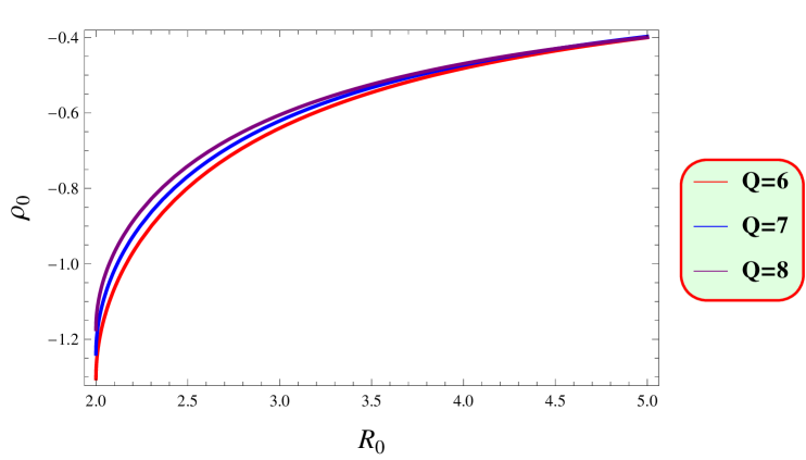
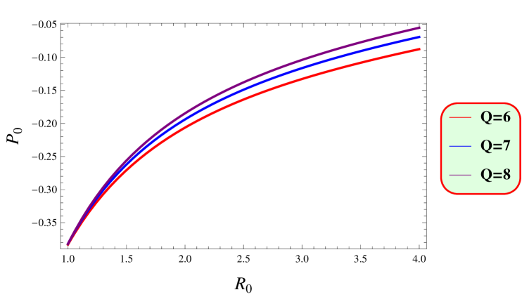
Figure 1: Plots of $\rho_{0}$ and $P_{0}$ for the RN Black Hole versus $R_{0}$.

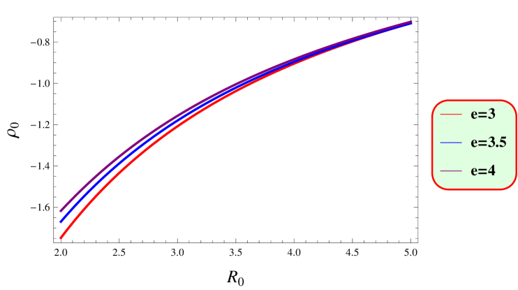
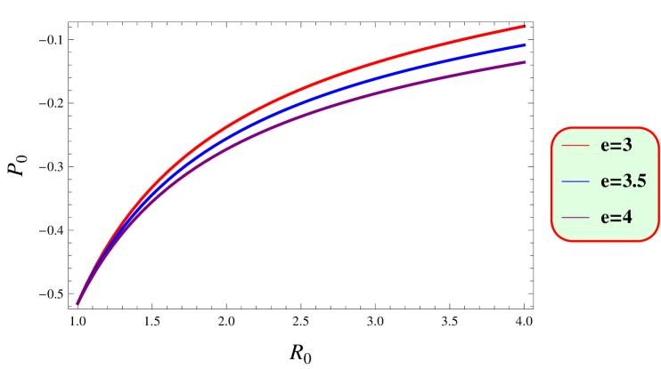
Figure 2: Graphs of $\rho_{0}$ and $P_{0}$ for the Bardeen Black Hole versus $R_{0}$.

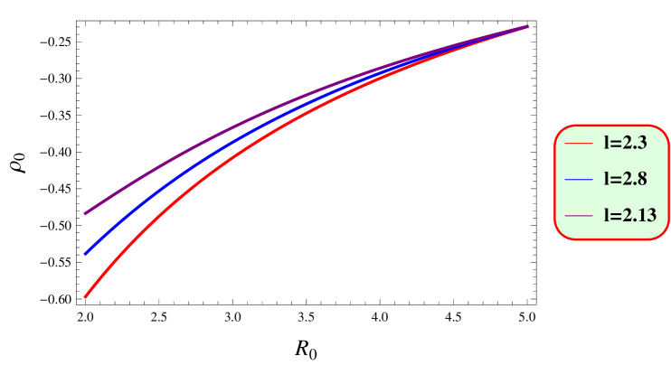
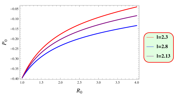
Figure 3: Graphs of $\rho_{0}$ and $P_{0}$ for the Hayward black hole versus $R_{0}$.

5 Physical Features of Charged Gravastar

This section will cover the physical properties of charged gravastar such as surface energy density, surface pressure, proper length, entropy, energy, the EoS parameter. We also discuss stability of the gravastar through the effective potential, causality condition and adiabatic index. We shall restrict ourselves to RN black hole only as the rest of the black holes provide complicated expressions and cannot be analyzed.

5.1 Proper length

According to Mazur and Mottola [21], the shell is situated at the boundary where two different spacetimes intersect. The shell stretches from the phase boundary at $r_{2}=R_{0}+\epsilon$, which separates the outer space-time from the intermediate thin-shell, to the phase barrier at $r_{1}=R_{0}$, which is located between the inner region and the intermediate thin-shell ( $\epsilon$ is the thickness of the shell and a small distance). The thickness of the shell is determined between these boundary points as [49]

$$L=\int_{R_{0}}^{R_{0}+\varepsilon}\sqrt{e^{\beta(R)}}dR.$$

This expression can be converted into the interior function as

$$L = \int_{R_{0}}^{R_{0}+\varepsilon}\bigg{(}\frac{\big{(}2R(R-2M)+Q^{2}\big{)}\big{(}\zeta R^{2}-2\psi\big{)}}{6Q^{2}\psi-4R^{2}\psi}-c_{1}\bigg{)}^{-1}dr,$$ (83)

which can also be written as (using Eq.(72))

$$L=\int_{R_{0}}^{R_{0}+\varepsilon}\frac{1}{\Phi_{-}(R)}dR.$$

Evaluating the integral in Eq.(83) is a bit challenging. To simplify the process, we take a particular assumption that $\frac{d\Phi_{-}(R)}{dR}=\frac{1}{\Phi_{-}(R)}$ and solve the integral, implying that

$$L=-\Phi_{-}(R_{0})+\Phi_{-}(R_{0}+\varepsilon).$$ (84)

Next, by expanding $V_{-}(R_{0}+\epsilon)$ into a Taylor series around $R_{0}$ and focusing only on the first order terms in $\epsilon$. Because $\epsilon$ is very small, we can ignore the higher order terms in the expansion. Figure 4 shows the behavior of proper length versus thickness. It shows that as the thickness increases, the proper length of the shell also increases consistently. This can be attributed to the changing geometric properties of the shell, where a greater thickness allows for a larger spatial extent. Understanding this relationship is crucial for assessing the structural integrity and physical behavior of the shell, particularly in how it responds to external forces and energy distributions.

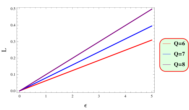
Figure 4: Graph of proper length versus thickness.

5.2 Entropy

The entropy $S$ for the intermediate thin-shell can be calculated as

$$S=\int_{R_{0}}^{R_{0}+\varepsilon}4\pi R^{2}s(R)\sqrt{e^{\beta(R)}}dR,$$ (85)

where the entropy density is represented by $s(R)$, and its mathematical expression is given as follows

$$s(R)=\frac{k^{2}(K_{B})^{2}\mathcal{T}(R)}{4\pi\hbar^{2}\mathcal{G}}=\frac{kK_{B}}{\hbar}\bigg{(}\frac{P_{0}}{2\pi\mathcal{G}}\bigg{)}^{\frac{1}{2}},$$ (86)

here, $k$ is non-zero arbitrary constant, $\mathcal{T}(R)$ represents the temperature, $\hbar$ and $K_{B}$ refer to Planck’s and Boltzmann’s constants, respectively. Here, we use the geometric units, where $G=1$. Consequently, Eq.(85) simplifies to

$$S = \int_{R_{0}}^{R_{0}+\varepsilon}4\pi R^{2}\frac{kK_{B}}{\hbar}\bigg{(}\frac{P_{0}}{2\pi}\bigg{)}^{\frac{1}{2}}\sqrt{e^{\beta(R)}}dR=\int_{R_{0}}^{R_{0}+\varepsilon}2\sqrt{2\pi}R^{2}\frac{kK_{B}}{\hbar}\sqrt{P_{0}e^{\beta(R)}}dR.$$

This expression can be further written as

$$S=2\sqrt{2\pi}R^{2}\frac{kK_{B}}{\hbar}N,$$ (87)

where

$$N=\int_{R_{0}}^{R_{0}+\epsilon}\sqrt{P_{0}e^{\beta(R)}}dR=\int_{R_{0}}^{R_{0}+\epsilon}D(R)dR.$$ (88)

According to Eq.(88), calculating the integral directly is quite difficult at this stage. If we consider $F(R)$ as the integral of $D(R)$, we can proceed with the calculation. Using this approach, Eq.(88) is simplified after applying the fundamental theorem of calculus. The result is

$$N=[F(R)]_{R_{0}}^{R_{0}+\epsilon}=F(R_{0}+\epsilon)-F(R_{0}).$$ (89)

When we keep only the linear terms of $\epsilon$ and expand $F(R_{0}+\epsilon)$ using a Taylor series around $d$, we find (using Eq.(87)) that

$$S = \bigg{[}\bigg{(}\frac{\big{(}2R_{0}(R_{0}-2M)+Q^{2}\big{)}\big{(}\zeta R_{0}^{2}-2\psi\big{)}}{6Q^{2}\psi-4R_{0}^{2}\psi}-c_{1}\bigg{)}\bigg{(}\sqrt{1-\frac{2M}{R_{0}}+\frac{Q^{2}}{R_{0}^{2}}}$$ (90)

$$- \sqrt{\frac{\big{(}2R_{0}(R_{0}-2M)+Q^{2}\big{)}\big{(}\zeta R_{0}^{2}-2\psi\big{)}}{6Q^{2}\psi-4R_{0}^{2}\psi}-c_{1}}+\frac{1}{8\pi}\bigg{(}\frac{1}{R_{0}^{2}}(MR_{0}-Q^{2}$$

$$\times \sqrt{R_{0}^{2}-2MR_{0}+Q^{2}})+\bigg{(}2Q^{2}\big{(}9\zeta MR_{0}^{2}-6M\psi-6\zeta R_{0}^{3}+8R_{0}\psi\big{)}$$

$$- 4M\big{(}\zeta R_{0}^{4}+2R_{0}^{2}\psi\big{)}-3\zeta Q^{4}R_{0}+4\zeta R_{0}^{5}\bigg{)}\bigg{(}\sqrt{2}\psi\big{(}3Q^{2}-2R_{0}^{2}\big{)}^{2}\bigg{(}\bigg{(}\big{(}2$$

$$\times c_{1}R_{0}\psi-2\zeta MR_{0}^{2}+4M\psi+\zeta R_{0}^{3}-2R_{0}\psi\big{)}2R_{0}+Q^{2}\big{(}\zeta R_{0}^{2}-2(3c_{1}\psi$$

$$+ \psi)\big{)}\bigg{)}\bigg{(}\psi\big{(}3Q^{2}-2R_{0}^{2}\big{)}\bigg{)}^{-1}\bigg{)}^{\frac{1}{2}}\bigg{)}^{-1}\bigg{)}\bigg{)}\bigg{]}^{\frac{1}{2}}\frac{\big{(}R_{0}^{2}kK_{B}\epsilon\big{)}}{\sqrt{4}\hbar}.$$

Figure 5 shows that the disorder within the gravastar increases as the shell’s thickness expands, with the entropy rising in proportion to the shell’s thickness and peak at the outer surface. A shell with no thickness results in zero entropy. Moreover, as the charge increases, the level of disorder also increases, which helps in forming a more stable structure. The model parameter affects entropy as well, with positive values leading to higher entropy than negative ones. This indicates that the outer layers are more disordered compared to the inner layers. Thus, increasing charge enhances the disorder within the gravastar, further promoting structural stability.

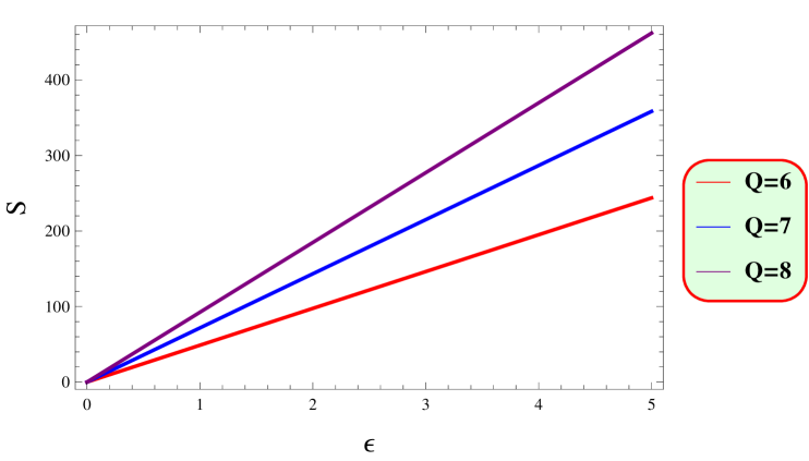
Figure 5: Graph of entropy versus thickness.

5.3 Energy

We can find the energy of the shell

$$E=\int_{R_{0}}^{R_{0}+\varepsilon}4\pi R^{2}\rho_{0}dR.$$ (91)

Using Eqs.(32) and (31), it follows that

$$E=\frac{4\pi\epsilon^{3}}{3}\bigg{(}\frac{\sqrt{-\frac{2M}{R_{0}}+\frac{Q^{2}}{R_{0}^{2}}+1}-\sqrt{\frac{\big{(}2R_{0}(R_{0}-2M)+Q^{2}\big{)}\big{(}\zeta R_{0}^{2}-2\psi\big{)}}{6Q^{2}\psi-4R_{0}^{2}\psi}-c_{1}}}{4\pi R_{0}}\bigg{)}.$$ (92)

Figure 6 indicates that the energy of the shell increases with the shell thickness. In our model, the energy density is closely related to the pressure within the shell and a thicker shell allows for greater interactions between gravitational and electromagnetic forces, which influence the energy distribution.

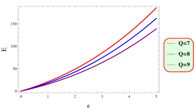
Figure 6: Graph of energy versus thickness.

5.4 The EoS Parameter

The EoS parameter can be expressed as

$$\omega = \bigg{[}\bigg{(}\sqrt{1-\frac{2M}{R_{0}}+\frac{Q^{2}}{R_{0}^{2}}}-\sqrt{\frac{\big{(}2R_{0}(R_{0}-2M)+Q^{2}\big{)}\big{(}\zeta R_{0}^{2}-2\psi\big{)}}{6Q^{2}\psi-4R_{0}^{2}\psi}-c_{1}}$$

$$+ \frac{1}{8\pi}\bigg{(}\frac{1}{R_{0}^{2}}(MR_{0}-Q^{2}\sqrt{R_{0}^{2}-2MR_{0}+Q^{2}})+\bigg{(}2Q^{2}\big{(}9\zeta MR_{0}^{2}-6M$$

$$\times \psi-6\zeta R_{0}^{3}+8R_{0}\psi\big{)}-4M\big{(}\zeta R_{0}^{4}+2R_{0}^{2}\psi\big{)}-3\zeta Q^{4}R_{0}+4\zeta R_{0}^{5}\bigg{)}\bigg{(}\sqrt{2}$$

$$\times \psi\big{(}3Q^{2}-2R_{0}^{2}\big{)}^{2}\bigg{(}\bigg{(}\big{(}2cR_{0}\psi-2\zeta MR_{0}^{2}+4M\psi+\zeta R_{0}^{3}-2R_{0}\psi\big{)}2R_{0}$$

$$+ Q^{2}\big{(}\zeta R_{0}^{2}-2(3c_{1}\psi+\psi)\big{)}\bigg{)}\bigg{(}\psi\big{(}3Q^{2}-2R_{0}^{2}\big{)}\bigg{)}^{-1}\bigg{)}^{\frac{1}{2}}\bigg{)}^{-1}\bigg{)}\bigg{)}\bigg{(}\frac{1}{4\pi R_{0}}$$

$$\times \bigg{(}\sqrt{1-\frac{2M}{R_{0}}+\frac{Q^{2}}{R_{0}^{2}}}-\sqrt{\frac{\big{(}2R_{0}(R_{0}-2M)+Q^{2}\big{)}\big{(}\zeta R_{0}^{2}-2\psi\big{)}}{6Q^{2}\psi-4R_{0}^{2}\psi}-c_{1}}\bigg{)}\bigg{)}^{-1}\bigg{]}.$$

The validity of different stellar models is effectively characterized by various EoS parameter values. For instance, $\omega=0$ corresponds to flat surfaces with non-relativistic fluid, $\omega=-\frac{1}{3}$ applies to curved surfaces, $\omega=-1$ is associated with DE, $\omega<-1$ signifies phantom energy and $\omega\geq-1$ defines the non-phantom regime. In the Figure 7, we observe that $\omega$ drops below -1, entering the phantom region, which shows the significance of the gravastar structure. This behavior implies a negative energy density associated with the gravastar, suggesting the possibility of repulsive gravitational effects that could contribute to the accelerated expansion of the universe. In contrast to conventional matter and energy, which have $\omega\geq-1$, gravastars’ ability to enter the phantom regime positions them as viable alternative models for explaining cosmic phenomena such as DE, that standard cosmological models struggle to address.

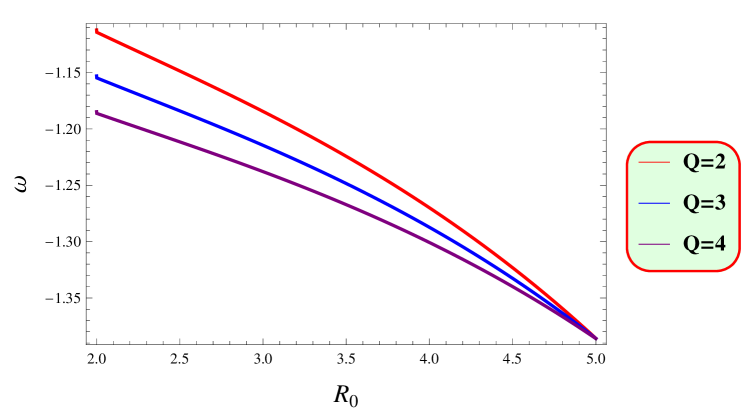
Figure 7: Graph of EoS versus $R_{0}$.

5.5 Stability Analysis

Here, we assess the stability of thin-shell gravastars by analyzing the potential function and its second derivative. A structure is considered stable when $V^{\prime\prime}(R_{0})>0$, unstable when $V^{\prime\prime}(R_{0})<0$, and unpredictable for $V^{\prime\prime}(R_{0})=0$. We give the graphical behavior of $V^{\prime\prime}(R_{0})$ for all the three black holes due to complicated expressions. Figures 8-10 confirm that $V^{\prime\prime}(R_{0})>0$ for three distinct values of $Q,~e$ and $l$, hence the stable configuration of thin-shell gravastars is achieved. A positive second derivative signifies that small perturbations in the configuration will generate restoring forces, returning the system to its equilibrium state. Thus, the gravastar configuration is stable against minor changes, whether caused by external influences or internal fluctuations.

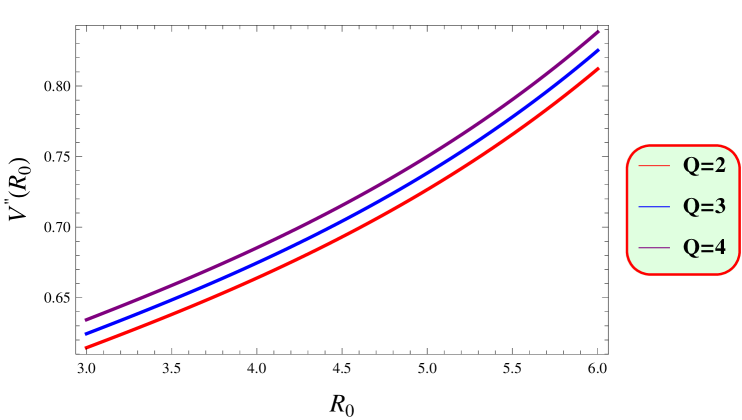
Figure 8: Potential for the shell beyond RN metric.

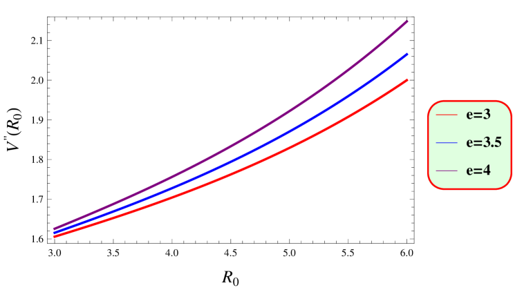
Figure 9: Potential for the shell beyond Bardeen black hole.

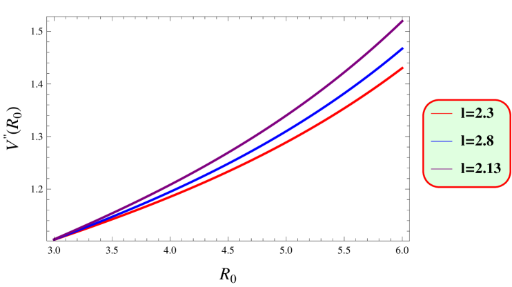
Figure 10: Potential for the shell beyond Hayward black hole.

Next, we discuss the stability analysis through causality condition and adiabatic index. In general fluids, the speed of sound, which measures how quickly disturbances move through the medium, can be expressed as

$$v_{s}^{2}=\frac{p^{\prime}}{\varrho^{\prime}},$$ (93)

where $\varrho$ and $p$ for the thin-shell are given in Eqs.(32) and (33), respectively. To find the speed of sound in thin-shell, this expression can be evaluated at $R$. Poisson and Visser [81] proposed that, due to causality, the speed of sound should not surpass the speed of light (with $c=1$ in natural units). Thus, the speed of sound $v_{s}^{2}$ is expected to fall within the range $0\leq v_{s}^{2}\leq 1$.

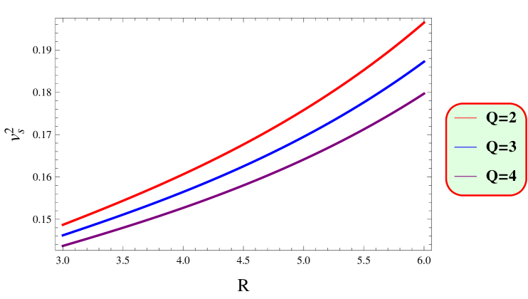
Figure 11: Graph of $v_{s}^{2}$ with respect to $R$ for different values of $Q$.

The stability of gravastars has been extensively analyzed using this criterion. For instance, Lobo [82] applied this approach to determine stability limits for a wormhole in the presence of a cosmological constant. Other studies [83] have also investigated the stability of charged gravastars. However, as mentioned in [81], there are some limitations of using the speed of sound for stability analysis. In the stiff matter region (where $\omega=1$), it is not entirely clear if Eq.(93) accurately represents the speed of sound. This uncertainty arises from the incomplete understanding of the microscopic properties of stiff matter, making the typical fluid argument potentially unreliable. Despite not being a complete condition, this method still provides a necessary condition for ensuring the stability of the thin-shell surrounding the gravastar. Inserting the required values in (93), we derive the result for $v_{s}^{2}$.

Figure 11 illustrates how the changes in $v_{s}^{2}$, in relation to the radial distance $R$ and different charge values, influence the stability of the gravastar’s shell. The fact that the condition $0\leq v_{s}^{2}\leq 1$ is satisfied indicates that the gravastar maintains stability under these conditions. Our analysis indicates that increasing charge affects both energy density and pressure distribution, subsequently influencing the $v_{s}^{2}$. This insight enhances our understanding of the gravastar’s physical behavior.

The adiabatic index $(\Gamma)$ is another factor for checking the stability of stars, including gravastars. It shows how pressure and density affect a star’s stability and is calculated using a specific formula

$$\Gamma=\frac{v_{s}^{2}(p+\varrho)}{p}.$$

To analyze stability, it is important to find the value of $\Gamma$. For an object to be stable, $\Gamma$ should be greater than 4/3. If $\Gamma$ drops below this value, the object becomes unstable and can collapse [84].

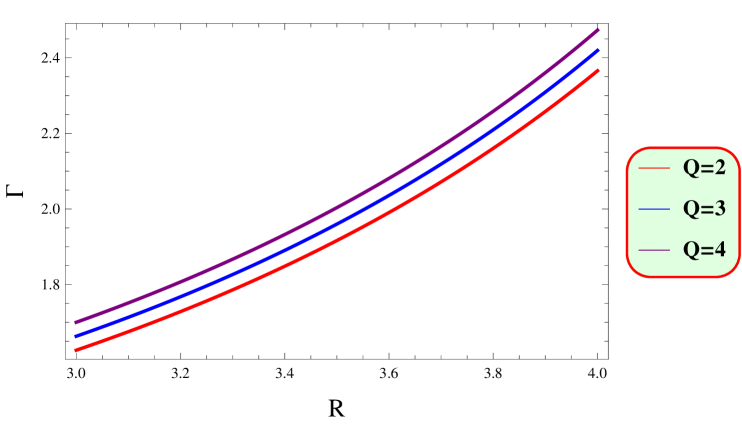
Figure 12: Variation of $\Gamma$ with respect to $R$ for different values of $Q$.

Figure 12 demonstrates that our system remains stable, as it fulfills the required limit ($\Gamma>\frac{4}{3}$). Thus, we achieve a viable and stable gravastar. This condition ensures that the gravastar can maintain its structure against gravitational collapse and energy dissipation. Our analysis emphasizes key parameters influencing stability such as energy density and pressure, along with their interrelationships.

6 Summary and Discussion

In this paper, we have investigated a charged gravastar solution using the Finch-Skea metric within the framework of $f(\mathbb{Q})$ gravity. To gain a deeper understanding of the gravastar, we have examined three distinct regions: the interior core, the intermediate shell and the exterior vacuum, each governed by its own specific EoS parameter. We have analyzed key physical properties, including proper length, entropy, energy and the EoS parameter. The stability of the gravastar solution has been assessed through the effective potential, the causality condition and adiabatic index. We have identified several key aspects of the gravastar solutions, which are summarized as follows.

• We have found that both the increasing energy density and pressure indicate that the shell’s outer boundary is denser than its inner boundary (Figures 1-3).

• The proper length steadily increases with the shell’s thickness for different charge values. This illustrates a fundamental physical characteristic of the shell’s structure (Figure 4).

• We have found that the disorder within the gravastar increases as the shell’s thickness expands. Furthermore, higher values of charge and positive model parameters lead to greater entropy, contributing to a more stable structure (Figure 5).

• We have observed that the shell energy steadily increases with thickness, hence the gravastar remains in stable position (Figure 6).

• The EoS is found to drop below -1, moving into the phantom region for various charge values (Figure 7).

• The stable configuration of thin-shell gravastars has been checked using the condition $V^{\prime\prime}(R_{0})>0$, (Figures 8-10). We have also assessed the stability of the gravastar through speed of sound and adiabatic index and have found that the gravastar satisfies the stability criteria (Figure 11,12).

Gravastars have garnered significant attention in modified gravity theories due to their potential to offer alternative explanations for compact stellar structures. This study focuses on gravastars within the $f(\mathbb{Q})$ gravity framework, a theory renowned for its consistency with observational data and its capability to explain the universe accelerated expansion. Unlike GR, which relies heavily on DE, $f(\mathbb{Q})$ gravity provides a geometric foundation to address challenges such as cosmic acceleration and singularities. In this paper, gravastar models offer a distinct advantage by eliminating event horizons, thereby resolving the information loss paradox. These configurations are characterized by finite pressure and density, presenting them as stable and physically consistent alternatives to black holes. Furthermore, $f(\mathbb{Q})$ gravity enables a deeper exploration of gravitational and electromagnetic interactions, contributing to the broader understanding of compact astrophysical phenomena.

We have identified a set of viable solutions that successfully avoid the central singularities and event horizons typically associated with black holes. The presence of charge introduces an outward-directed force, providing a repulsive effect that prevents the gravastar from collapsing into a singularity. As a result, charged gravastar demonstrate greater stability compared to uncharged gravastar. Future research could delve further into gravastar solutions within the context of $f(\mathbb{Q})$ gravity. Our findings reveal a consistent enhancement of physical properties due to the influence of charge, in line with observations in GR and other modified gravity theories [85]-[86].

Building on this, we compare our findings with existing studies to highlight the novel contributions of our work. In a recent paper [49], Mohanty and Sahoo used the Krori-Barua metric in $f(\mathbb{Q})$ gravity to explore gravastar characteristics, such as proper length, entropy and stability condition. Our analysis emphasizes significant role of charge in enhancing gravastar stability. We show that higher charge values increase entropy and stability, providing a more understanding of gravastar behavior as compared to Mohanty and Sahoo. Shamir and Ahmad [32] examined gravastars in $f(\mathbb{G},T)$ gravity and found that their study does not emphasize the repulsive forces introduced by charge, a critical aspect in our study. Yousaf et al. [87] explored charged gravastars in $f(\mathbb{R},T)$ gravity, focusing on the role of electromagnetic fields in gravastar stability. Sharif and Naz [58] studied gravastars in $f(\mathbb{R},T^{2})$ gravity using the Finch-Skea metric. Our work not only aligns with these findings but also extend them by providing a clearer correlation between charge and enhanced stability in the $f(\mathbb{Q})$ context.

The treatment of the Finch-Skea metric significantly influences the results by simplifying field equations and ensuring singularity-free solutions. It maintains regularity at the center, smooth matching between regions, and stability of energy density and pressure profiles, even with the inclusion of charge. Through Israel junction conditions, surface energy density and pressure are accurately calculated, ensuring physical consistency. Its compatibility with exterior geometries enables unified solutions for charged configurations. In this work, we have analyzed key physical quantities such as proper length, entropy, energy density, pressure, and EoS parameter, specifically at equilibrium, along with stability indicators like the causality condition and adiabatic index, within this gravity. While these analyses align with established theoretical approaches, they offer new insights into the stability and equilibrium of the gravastar model. Our graphical results further confirm that the proposed model is both stable and theoretically viable.

Data Availability Statement: No data was used for the research described in this paper.

References

- [1] Riess, A.G. et al.: Astron. J. 116(1998)1009; Perlmutter, S. et al.: Astrophys. J. 517(1999)565.
- [2] Sahni, V. and Starobinski, A.: Int. J. Mod. Phys. D 9(2000)373.
- [3] Yang, R.J. and Zhang, S.N.: Mon. Not. R. Astron. Soc. 407(2010)1835.
- [4] Velten, H.E.S. et al.: Eur. Phys. J. C 74(2014)3160.
- [5] Wang, D. et al.: Eur. Phys. J. C 79(2019)211; Mandal, S. et al.: Phys. Dark Uni. 28(2020)100551; Yerramsetti, Y. et al.: Eur. Phys. J. C 79(2020)1020; Wang, D.: Phys. Dark Uni. 28(2020)100545; Arora, S. et al.: Class. Quantum Grav. 37(2020)205022.
- [6] Cartan, .: C.R. Acad. Sci. 174(1922)593.
- [7] Buchdahl, H.A.: Month. Not. R. Astron. Soc. 150(1970)1; Aldrovandi, R. and Pereira, J.G.: Teleparallel Gravity: An Introduction (Springer, 2013); Maluf, J. W.: Ann. Phys. 525(2013)339.
- [8] Adak, M. et al.: Int. J. Mod. Phys. A 28(2013)1350167; Mol, I.: Adv. Appl. Clifford Algebras 27(2017)2607; Jrv, L. et al.: Phys. Rev. D 97(2018)124025.
- [9] Jimenez, J.B., Heisenberg, L. and Koivisto, T.: Phys. Rev. D 98(2018)044048.
- [10] Conroy, A. and Koivisto, T.: Eur. Phys. J. C 78(2018)923; Delhom-Latorre, A., Olmo, G.J. and Ronco, M.: Phys. Lett. B 780(2018)294; Hohmann, M. et al.: Phys. Rev. D 99(2019)024009.
- [11] Harko, T. et al.: Phys. Rev. D 98(2018)084043.
- [12] Lazkoz, R. et al.: Phys. Rev. D 100(2019)104027.
- [13] Mandal, S., Sahoo, P.K. and Santos, J.R.: Phys. Rev. D 102(2020)024057.
- [14] Lin, R.H. and Zhai, X.H.: Phys. Rev. D 103(2021)124001.
- [15] Mandal, S. and Sahoo, P.K.: Phys. Lett. B 823(2021)136786.
- [16] Lymperis, A.: J. Cosmol. Astropart. Phys. 11(2022)018.
- [17] Koussour, M. et al.: Prog. Theor. Exp. Phys. 2023(2023)113E01.
- [18] de Araujo, J.C. and Fortes, H.G.M.: arXiv:2407.08884.
- [19] Sharif, M. and Ajmal, M.: Chin. J. Phys. 88(2024)706; Phys. Scr. 99(2024)085039.
- [20] Sharif, M. and Ajmal, M.: Phys. Dark Uni. 46(2024)101572.
- [21] Mottola, E. and Mazur, P.O.: Gravitational Condensate Stars: An Alternative to Black Holes (In APS April Meeting Abstracts, 2002); Mazur, P.O. and Mottola, E.: Proc. Natl. Acad. Sci. 101(2004)9545.
- [22] Carter, B.M.N.: Class. Quantum Grav. 22(2005)4551; Lobo, F.S.N.: Class. Quantum Grav. 23(2006)525; DeBenedictis, A.: Class. Quantum Grav. 23(2006)2303.
- [23] Lobo, F.S.N. and Arellano, A.V.B.: Class. Quantum Grav. 24(2007)1069; Rocha, P. : J. Cosmol. Astropart. Phys. 11(2008)010.
- [24] Bhar, P.: Astrophys. Space Sci., 354(2014)2109; Rahaman, F. et al.: Int. J. Theor. Phys. 54(2015)50; D’Ambrosio, F. et al.: Phys. Rev. D 105(2022)024042.
- [25] Visser, M. and Wiltshire D.L.: Class. Quantum Grav. 21(2004)1135; Cattoen, C., Faber, T. and Visser, M.: Class. Quantum Grav. 22(2005)4189.
- [26] Bili’c, N., Tupper, G.B. and Viollier, R.D.: J. Cosmol. Astropart. Phys. 02(2006)013; Horvat, D. and Iliji’c, S.: Class. Quantum Grav. 24(2007)5637.; Chirenti, C.B.M.H. and Rezzolla, L.: Class. Quantum Grav. 24(2007)4191.
- [27] Nandi, K.K. etal. Phys. Rev. D 79(2009)024011; Turimov, B.V., Ahmedov, B.J. and Abdujabbarov, A.A.: Mod. Phys. Lett. A 24(2009)733; Usmani, A.A.: Phys. Lett. B 701(2011)388.
- [28] Clifton, T. et al.: Phys. Rep. 513(2012)1; Lobo, F.S.N. and Garattini, R.: J. High Energy Phys. 12(2013)065.
- [29] Sakai, N. et al.: Phys. Rev. D 90(2014)104013.
- [30] Kubo, T. and Sakai, N.: Phys. Rev. D 93(2016)084051.
- [31] Das, A. et al.: Phys. Rev. D 95(2017)124011.
- [32] Shamir, M.F. and Ahmad, M.: Phys. Rev. D 97(2018)104031.
- [33] Bhatti, M.Z., Yousaf, Z. and Rehman, A.: Phys. Dark Univ. 29(2020)100561.
- [34] Sengupta, R. et al.: Phys. Rev. D 102(2020)024037.
- [35] Bhatti, M.Z. et al.: Indian J. Phys. 98(2024)1901.
- [36] Sinha, M. and Singh, S.S.: arXiv:2407.09579.
- [37] Teruel, G.R.P. et al.: Phys. Dark Univ. 43(2024)101404.
- [38] Sharif, M., Naseer, T. and Tabassum, A.: Chin. J. Phys. 92(2024)579.
- [39] vgn, A. et al.: Eur. Phys. J. C 77(2017)1.
- [40] Sharif, M. and Waseem, A.: Astrophys. Space Sci. 364(2019)189.
- [41] Bhar, P. and Rej, P.: Eur. Phys. J. C 81(2021)1.
- [42] Barzegar, H. et al.: Eur. Phys. J. C 83(2023)151.
- [43] Ilyas, M., Athar, A. R. and Bibi, A.: New Astron. 103(2023)102053.
- [44] Bhar, P.: Chin. J. Phys. 85(2023)600.
- [45] Bhattacharjee, D. and Chattopadhyay, P.K.: Phys. Scr. 98(2023)085013.
- [46] Bhattacharjee, D. and Chattopadhyay, P.K.: J. High Energy Astrophys. 43(2024)248.
- [47] Gogoi, D.J. et al.: Eur. Phys. J. C 83(2023)700.
- [48] Pradhan, S., Mandal, S. and Sahoo, P.K.: Chin. Phys. C 47(2023)055103.
- [49] Mohanty, D. and Sahoo, P.K.: Fortschr. Phys. 72(2024)2400082.
- [50] Javed, F. et al.: Chin. J. Phys. 90(2024)421.
- [51] Mohanty, D., Ghosh, S. and Sahoo, P.K.: Ann. Phys. 463(2024)169636.
- [52] Sharma, R. and Ratanpal, B.S: Int. J. Mod. Phys. D 22(2013)1350074
- [53] Bhar, P. et al.: Commun. Theor. Phys. 62(2014)221.
- [54] Banerjee, A., Jasim, M.K. and Pradhan, A.: Mod. Phys. Lett. A 35(2020)2050071.
- [55] Dey, S. and Paul, B.C.: Class. Quantum Grav. 37(2020)075017.
- [56] Maurya, S.K. et al.: Eur. Phys. J. C 82(2022)1.
- [57] Majeed, K., Abbas, G. and Siddiqa, A.: New Astron. 95(2022)101802.
- [58] Sharif, M. and Naz, S.: Mod. Phys. Lett. A 38(2023)2350123.
- [59] Dayanandan, B. et al.: Chin. J. Phys. 82(2023)155.
- [60] Sharif, M. and Manzoor, S.: Ann. Phys. 454(2023)169337.
- [61] Gul, M.Z. et al.: Eur. Phys. J. C 84(2024)8.
- [62] Mustafa, G. et al.: Chin. J. Phys. 88(2024)954.
- [63] Karmakar, A., Debnath, U. and Rej, P.: Chin. J. Phys. 90(2024)1142.
- [64] Rej, P., Bogadi, R.S. and Govender, M.: Chin. J. Phys. 87(2024)608.
- [65] Shahzad, M.R. et al.: Phys. Dark Univ. 46(2024)101646.
- [66] Das, B. et al.: Astrophys. Space Sci. 369(2024)76.
- [67] Gul, M. Z., Sharif, M. and Arooj, A.: arXiv:2408.15389.
- [68] Novello, M. and Perez Bergliaffa, S.E.: Phys. Rep. 463(2008)127.
- [69] Hehl, F.W. et al.: Rev. Mod. Phys. 48(1976)393.
- [70] Sharif, M. and Ibrar, I.: Chin. J. Phys. 89(2024)1578; Sharif, M. and Ajmal, M.: Phys. Scr. 99(2024)085039; Astropart. Phys. 165(2025)103054.
- [71] Goncalves, V.P. and Lazzari, L.: Phys. Rev. D 102(2020)034031.
- [72] Bhattacharjee, D. and Chattopadhyay, P.K.: arXiv:2407.10587.
- [73] Finch, M.R. and Skea, J.E.F.: Class. Quantum Grav. 6(1989)467.
- [74] Zel′dovich, Y.B.: Mon. Not. R. Astron. Soc. 160(1972)1P.
- [75] Staelens, F. et al.: Gen. Relativ. Gravit. 53(2021)1.
- [76] Carr, J.B.: Astrophys. J. 201(1975)1; Madsen, M.S. et al.: Phys. Rev. D 46(1992)1399; Braje, T.M. et al.: Astrophys. J. 580(2002)1043; Ferrari, L. et al.: Int. J. Mod. Phys. E 16(2007)2834; Rahaman, F. et al.: Eur. Phys. J. C 74(2014)2845.
- [77] Israel, W.: Nuo. Cim. B 44(1966)1.
- [78] Sen, N.: Ann. Phys. 378(1924)365.
- [79] Darmois, G. et al.: Mmorial des sciences mathmatiques (Gauthier-Villars Paris, 1927).
- [80] Israel, W.: Nuo. Cim. B 48(1967)463.
- [81] Poisson, E. and Visser, M.: Phys. Rev. D 52(1995)7318.
- [82] Lobo, F.S.N. and Crawford, P.: Class. Quantum Grav. 21(2003)391.
- [83] Bhar, P. and Rej, P.: Eur. Phys. J. C 81(2021)763; Debnath, U. et al.: Eur. Phys. J. Plus 136(2021)1.
- [84] Chandrasekhar, S.: Astrophys. J. 140(1964)417; Chan, R., Herrera, L. and Santos, N.: Mon. Not. R. Astron. Soc. 265(1993)533.
- [85] Das, A. et al.: Nucl. Phys. B 954(2020)114986.
- [86] Shah, H. et al.: Phys. Scr. 98(2023)085246.
- [87] Yousaf, Z. et al.: Phys. Rev. D 100(2019)024062.