PriFFT: Privacy-preserving Federated Fine-tuning of Large Language Models via Function Secret Sharing

Abstract

Fine-tuning large language models (LLMs) raises privacy concerns due to the risk of exposing sensitive training data. Federated learning (FL) mitigates this risk by keeping training samples on local devices, but recent studies show that adversaries can still infer private information from model updates in FL. Additionally, LLM parameters are typically shared publicly during federated fine-tuning, while developers are often reluctant to disclose these parameters, posing further security challenges. Inspired by the above problems, we propose PriFFT, a privacy-preserving federated fine-tuning mechanism, to protect both the model updates and parameters. In PriFFT, clients and the server share model inputs and parameters by secret sharing, performing secure fine-tuning on shared values without accessing plaintext data. Due to considerable LLM parameters, privacy-preserving federated fine-tuning invokes complex secure calculations and requires substantial communication and computation resources. To optimize the efficiency of privacy-preserving federated fine-tuning of LLMs, we introduce function secret-sharing protocols for various operations, including reciprocal calculation, tensor products, natural exponentiation, softmax, hyperbolic tangent, and dropout. The proposed protocols achieve up to $4.02\times$ speed improvement and reduce $7.19\times$ communication overhead compared to the implementation based on existing secret sharing methods. Besides, PriFFT achieves a $2.23\times$ speed improvement and reduces $4.08\times$ communication overhead in privacy-preserving fine-tuning without accuracy drop compared to the existing secret sharing methods.

I Introduction

Large language models (LLMs), such as GPT-4 [1], Llama [2], and BERT [3], are pre-trained on natural language data to understand the structure, grammar, semantics, and more complex language patterns and concepts of language. Due to the advantages of the LLM parameter scale, LLMs are widely used in search engines, healthcare, finance, and other fields. Fine-tuning pre-trained LLMs according to downstream tasks allows LLMs to achieve higher accuracy and improved performance in specific domains. However, the training samples of downstream tasks contain sensitive information, causing privacy leakage concerns when fine-tuning LLMs in downstream tasks [4]. For example, fine-tuning LLMs for the medical domain involves direct access to patient disease information and medical records. Therefore, it is essential to prevent sensitive data leakage while enhancing model performance in fine-tuning LLMs.

Federated Learning (FL) [5] can protect sample data during model training. In FL, models are trained locally on the data owner’s side, and only model parameters are exchanged. The training data remains local, and the model developer never gets the original training data, which provides privacy protection for sensitive sample data. Therefore, fine-tuning LLMs with FL, i.e., federated fine-tuning, provides privacy preservation for training data in downstream tasks [6]. Figure 1 presents the framework of fine-tuning LLMs with FL where training samples remain local and only model updates are exchanged in the training process. Federated fine-tuning freezes most of the model’s parameters and fine-tunes LLMs by adjusting a few selected parameters, alleviating the issue of limited computational resources for clients in FL.

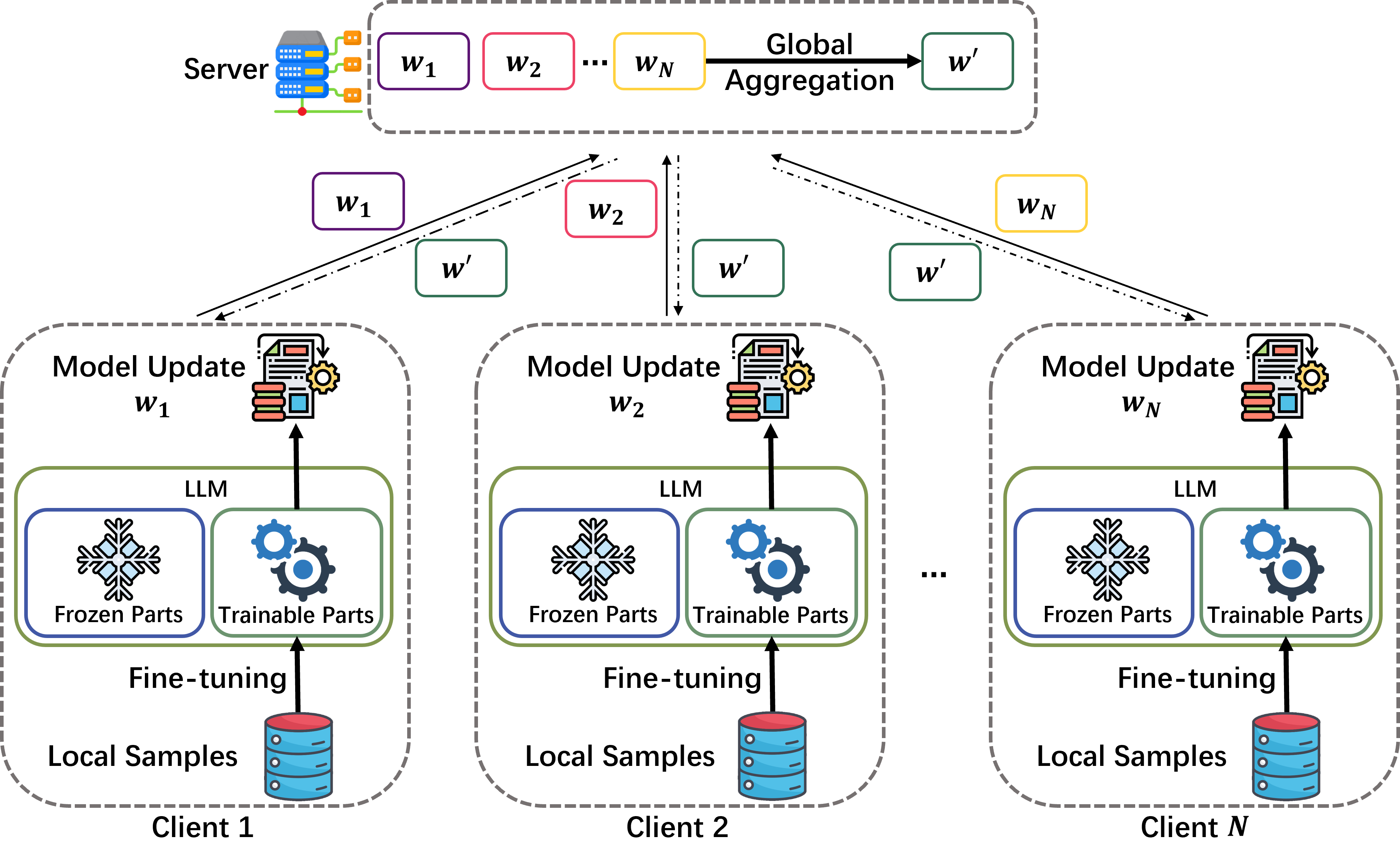
Figure 1: A simple framework of federated fine-tuning.

Motivation. Federated fine-tuning faces security threats from privacy leakage of model updates and parameter exposure of trained models. (i) Although the server cannot directly access training samples, attacks against FL show that the server can still infer training sample information through model updates [7]. For example, model inversion attacks [8] reconstruct training samples through model gradients uploaded by clients, presenting the privacy risks of uploading model updates generated by local samples to the server. (ii) Granting clients direct access to trained model parameters in FL raises concerns about intellectual property. Since model developers invest substantial computational resources, money, and effort in model training, they are cautious about disclosing trained model parameters to protect intellectual property and avoid commercial competition risks [9].

Existing privacy-preserving FL [10] mitigates the above privacy threats by implementing secure aggregation via secure multi-party computation (SMPC) [11]. Specifically, clients train the global model with local samples and generate model updates in plaintext. In the secure aggregation, the model updates are encrypted or perturbed before uploading. The server performs the model aggregation on the protected model updates with SMPC and generates updated global models. In the aggregation stage, the server cannot access the model updates, preventing the server from performing inference attacks on model updates and protecting clients’ sample security. However, the secure aggregation still requires model parameters to be exposed to clients, which cannot provide privacy-preserving for model parameters.

Challenges. Providing privacy-preserving for both model updates and parameters in federated fine-tuning of LLMs through SMPC faces computational and communication overhead challenges. (i) The extensive parameter scale of LLMs escalates the computation of model training, leading to a substantial increase in the training time for encryption-based FL mechanisms [12]. (ii) The increasing computation complexity of fine-tuning LLMs raises the communication overhead for inference and backpropagation in privacy-preserving FL mechanisms. In FL, clients possess fewer computing resources and less stable network communications than the server [13]. Consequently, addressing the computational and communication overhead is crucial for privacy-preserving federated fine-tuning of LLMs.

In this paper, we propose PriFFT, a privacy-preserving federated fine-tuning framework via function secret sharing (FSS) [14] to protect both model updates and parameters. To address the challenges of complex non-linear computations, we propose SMPC-friendly secure computation protocols leveraging FSS. These protocols reduce communication overhead by lowering both the number of communication rounds and the size of transmitted data. Built upon these proposed protocols, PriFFT significantly decreases the overall communication and computation burdens in privacy-preserving federated fine-tuning. PriFFT leverages GPU acceleration to further reduce execution time. Compared to the fine-tuning under plaintext data, the evaluation shows that PriFFT causes a minor drop in model accuracy while providing privacy-preserving for both model parameters and updates. Meanwhile, PriFFT significantly reduces communication and computation overhead compared to implementations based on ABY2 [15].

The contributions of this paper are summarized as follows:

• Privacy-preserving federated fine-tuning of LLMs. PriFFT is the first privacy-preserving FL mechanism for fine-tuning pre-trained LLMs according to downstream tasks. PriFFT enables federated fine-tuning of LLMs while protecting local samples and model updates of clients, as well as the parameters of trained model.

• Efficient implementation of complex computations. Dealing with the substantial complex secure computations in fine-tuning, we propose efficient computation protocols, including reciprocal calculation, tensor product, natural exponential, softmax, hyperbolic tangent, and dropout functions. Compared to the protocols implemented by ABY2, the proposed FSS-based protocols achieve up to 4.02$\times$ speed improvement and reduce 7.19$\times$ communication overhead with the same accuracy.

• Theoretical and experimental validity proof. We ensure the security and efficiency of PriFFT through theoretical analysis. Evaluation results on real standard datasets demonstrate that PriFFT realizes comparable model accuracy to plaintext training while protecting both model parameters and updates. With the same model accuracy of the ABY2 implementation, PriFFT achieves a 2.23$\times$ speed improvement and reduces 4.08$\times$ communication overhead. Within $1\%$ loss of accuracy in fine-tuned models, PriFFT achieves a 5.43$\times$ speed improvement and reduces 20.05$\times$ communication overhead.

The rest of this paper is organized as follows. Section II summarizes the related work. Section III and Section IV provide the preliminaries and a system overview, respectively. Section V presents the design of PriFFT. Section VI discusses the complexity and provides the security proofs of PriFFT. Section VII evaluates PriFFT through comprehensive experiments. Finally, Section VIII concludes the paper.

II Related Work

II-A Federated Fine-tuning of LLMs

Several existing works propose FL mechanisms to fine-tune LLMs and protect clients’ sample data. Qin et al. introduce zeroth-order optimization (ZOO) to realize full-parameter tuning of LLMs [16]. ZOO may struggle to achieve the same accuracy and efficiency as backpropagation when performing full-parameter fine-tuning of LLMs, since ZOO cannot precisely adjust model parameters by gradients. FedAdapter [17] implements adapter-based fine-tuning of LLMs with FL, which embeds adapters into LLMs and only optimizes adapter parameters according to downstream tasks. FedPETuning [18] develops a benchmark for four LLM fine-tuning methods, including adapter tuning, prefix tuning, and LoRA. FedPrompt [19] embeds soft prompts into global models and only adjusts the soft prompt parameters during the training process to realize communication-efficient fine-tuning of LLMs.

Exiting works on fine-tuning LLMs with FL do not provide privacy preservation for both model parameters and clients’ model updates. As clients fine-tune models on local devices in FL, the server must distribute model parameters to clients, leading to the exposure of these trained parameters. Model developers are cautious about disclosing trained model parameters due to potential intellectual property issues and commercial competition. Besides, clients fine-tune models and generate model updates based on the sample data specific to downstream tasks. The server can directly access the model updates in model aggregation and reconstruct training samples through model inversion attacks [7] using model updates, presenting the privacy leakage risk when uploading model updates in plaintext.

II-B Privacy-preserving Federated Learning

Existing privacy-preserving FL mechanisms provide protection for model updates through different secure strategies, including differential privacy (DP), encrypted aggregation, secret sharing, and trusted execution environment (TEE).

DP-based FL mechanisms protect model updates and parameters by adding noise to the sensitive data [20]. Clients perturb model updates with noise before uploading the model updates. Similarly, the server perturbs model parameters before distributing the parameters. Both clients and the server receive perturbed sensitive data with noise, achieving privacy preservation for model updates and parameters. However, noise in perturbed model updates and parameters brings drops in model performance. When fine-tuning LLMs with extensive parameters, the perturbation noise in model updates and parameters significantly impacts model accuracy.

In encrypted aggregation, model updates are transmitted in ciphertext, preventing the server from accessing the sensitive data in plaintext. BatchCrypt [12] employs homomorphic encryption (HE) to implement secure aggregation, in which gradients are encrypted via HE and gradient aggregation is realized through secure computation. Tamer et al. present a privacy-preserving FL based on symmetric encryption, addressing the clients’ dropout problem and enabling clients to validate the aggregated models [21]. SAFELearn [22] presents a communication-efficient and privacy-preserving FL framework that can be instantiated with SMPC or HE to defend model inversion attacks against model updates. Abbas et al. present an HE-based privacy-preserving FL against model poisoning attacks with an internal auditor and Byzantine-tolerant gradient aggregation [23]. Few existing works of encryption-based FL consider the privacy leakage issues related to model parameters. When model parameters are encrypted, the models’ local training must be done through secure computation. Fine-tuning LLMs with extensive encrypted parameters in FL imposes a significant computational load on clients.

The key idea of secret sharing-based FL mechanisms is to split model updates into multiple shares. Aggregation results are computed on shares, preventing the server from accessing clients’ gradients during the aggregation. FastSecAgg [24] combines multi-secret sharing and fast Fourier transform to realize a trade-off between the number of secrets, privacy threshold, and dropout tolerance. ELSA [25] introduces two servers in FL and splits clients’ gradients into two shares. Each server receives a share of clients’ gradients and performs gradient aggregation on received shares. VerSA [26] utilizes key agreement protocols to generate seeds for pseudorandom number generators, which are then used to generate masks for model updates. The aggregated results on masked model updates can offset the random values of the masks. Additionally, the secret sharing mechanism in VerSA addresses the issue of client dropout. Secret sharing-based FL mechanisms for fine-tuning of LLMs present significant communication overhead challenges, as the non-linear computations in fine-tuning of LLMs require extensive communication between clients and the server. Considering the limited communication capabilities of clients’ devices, clients may not be able to bear the communication consumption of FL mechanisms that directly apply secret sharing for privacy preservation.

Recently, Huang et al. combine TEE to realize privacy-preserving fine-tuning in which trainable parameters are put into the TEE during the fine-tuning process [27]. TEE guarantees the security of the proposed mechanism. However, the model parameters in TEE are plaintext. TEE is deemed not to provide provable security [28]. Therefore, the plaintext model parameters in TEE may confront privacy leakage.

This paper presents PriFFT to protect model parameters and updates with provable security while reducing computation and communication overhead in fine-tuning LLMs.

III Preliminary

III-A Federated Learning

In the training initialization phase, the server designs model structure $f$ with initialed parameter $\omega_{0}$, which is distributed to clients. In the $t$-th training round, clients download the latest model parameters $\omega_{t}$ and update local models. Assume that $N$ clients participate in FL training, the local training data of client $i\in\left[1,\cdots,N\right]$ are samples $x_{i}$ and labels $y_{i}$. The inference results are $f(x_{i};w_{t})$. Given the loss function $L$, the loss of client $i$ in local training is $L(f(x_{i};w_{t}),y_{i})$, and gradients are $g_{i}=\partial L(f(x_{i};w_{t}),y_{i})/\partial\omega_{t}$.

Clients upload gradients $g_{i}$ to the server in the aggregation phase of the $t$-th training round. The server averages gradients to get aggregated gradients as $\bar{g}=\sum_{i=1,\cdots,N}g_{i}$ and optimizes the parameters of the global models by aggregated gradients $\bar{g}$. The global model’s updated parameters $\omega_{t+1}$ are distributed to clients for the subsequent round of local training. The training process is terminated once a specified number of training rounds has been completed.

III-B Arithmetic Secret Sharing

We consider that secure computations are performed in the ring $\mathbb{Z}_{2^{l}}$, and all computations are modulo $2^{l}$, where $l$ is the bitwidth of the ring. We map a real number $x_{r}\in\mathbb{R}$ to the item of the ring $x\in\mathbb{Z}_{2^{l}}$ by $x=\left\lfloor x_{r}\cdot 2^{s}\right\rfloor\;\mathrm{mod}\;2^{l}$ where $s$ is a scale factor. The plaintext values are additively shared, and each party cannot learn information from the plaintext. Due to the space limitation, the sharing semantics and operations of ASS are given in the Appendix A-A.

III-C Function Secret Sharing

Due to communication efficiency, FSS has been applied in various areas to implement privacy-preserving mechanisms [29, 30, 31]. We consider a 2-party FSS scheme in this paper. Given a function family $\mathcal{F}$, FSS splits a function $f:\mathbb{G}^{\mathrm{in}}\rightarrow\mathbb{G}^{\mathrm{out}}$ into two additive shares $\{f_{0},f_{1}\}$ such that $f_{0}\left(x\right)+f_{1}\left(x\right)=f\left(x\right)$ where $x\in\mathbb{G}^{\mathrm{in}}$ and $f\left(x\right)\in\mathbb{G}^{\mathrm{out}}$. The security property of FSS requires that each share $f_{b}$ hides $f$. The formal definition of FSS and the key generation in the offline stage are given in Appendix A-B.

The evaluation $\mathrm{Eval}(\sigma,k_{\sigma},x)$ of FSS involves public input $x$, which is inconsistent in protecting sensitive data in privacy-preserving FL. Boyle et al. present secure evaluations in FSS based on offset functions [32]. The key idea is that for each gate $g:\mathbb{G}^{\mathrm{in}}\rightarrow\mathbb{G}^{\mathrm{out}}$ in the computation circuit, the input wire $w_{i}$ and output wire $w_{j}$ are masked by random offsets $r_{i}$ and $r_{j}$. Specifically, offset functions $\hat{\mathcal{G}}$ includes functions of the form $g^{\left[r^{\mathrm{in}},r^{\mathrm{out}}\right]}(x)=g(x-r^{\mathrm{in}})+r^{\mathrm{out}}$. Each party evaluates FSS shares on the common masked input $w_{i}+r_{i}$ and obtains additive shares of the masked output $w_{j}+r_{j}$ to get the correct shares. The formal definition of FSS with the offset function is given in Appendix A-B. In this paper, $\hat{x}$ refers to the fact that $x$ is masked by an offset $r$, i.e., $\hat{x}=x+r$. The notation $\left\langle\hat{x}\right\rangle_{b}$ refers to an additive share of $\hat{x}$ held by party $b\in{0,1}$.

Definition 1 (DPF [14]).

A distributed point function is an FSS scheme for the class of point functions $f_{\alpha,\beta}:\{0,1\}^{l}\rightarrow\mathbb{G}^{\mathrm{out}}$ which satisfy $f_{\alpha,\beta}(\alpha)=\beta$, and $f_{\alpha,\beta}(x)=0$ for any $x\neq\alpha$.

Given a pseudorandom generator (PRG) $G:\{0,1\}^{\lambda}\rightarrow\{0,1\}^{2\lambda+2}$, there exists a DPF for $f_{\alpha,1}:\mathbb{G}^{\mathrm{in}}\rightarrow\mathbb{G}^{\mathrm{out}}$ with key size $l\cdot(\lambda+2)+\lambda+\left\lceil\log_{2}|\mathbb{G}^{\mathrm{out}}|\right\rceil$ [33]. In this article, we apply the DPF-based comparison protocol proposed in SIGMA [34] to implement the secure comparison of shares.

III-D Share Conversion

The proposed privacy-preserving federated fine-tuning involves hybrid secure computing protocols based on ASS and FSS. The values are shared by ASS ($\left\langle x\right\rangle$) as discussed in Section III-B by default. When executing FSS-based protocols, the input of secure computing is $\left\langle\hat{x}\right\rangle$ which is then used to derive $\hat{x}$. The conversion process is defined as follows:

Conversion from $\left\langle x\right\rangle$ to $\left\langle\hat{x}\right\rangle$ is implemented by having each party to perform $\left\langle\hat{x}\right\rangle=\left\langle x\right\rangle+\left\langle r^{\mathrm{in}}\right\rangle$. FSS-based protocols first perform the conversion to obtain $\left\langle\hat{x}\right\rangle$. Some FSS-based protocols invoke $\left\langle r^{\mathrm{in}}\right\rangle$ to obtain computation results. To ensure that each party cannot infer information about $x$ from $\left\langle\hat{x}\right\rangle_{b}$, we split $r^{\mathrm{in}}$ twice in input conversion and offline stages.

Conversion from $\left\langle\hat{x}\right\rangle$ to $\left\langle x\right\rangle$ is required when an ASS-based protocol follows an FSS-based protocol. The conversion is implemented by omitting $\left\langle r^{\mathrm{out}}\right\rangle$ in the output of an FSS-based protocol. Without $\left\langle r^{\mathrm{out}}\right\rangle$, the output is converted to additive shares, while the key size is reduced $l$-bits due to the omission.

IV System Overview and Threat Model

IV-A Threat Model

Adversary’s identity. In this paper, we consider semi-honest servers and clients. The server and clients adhere to computation protocols while attempting to infer as much private information as possible from the calculation results.

Adversary’s goal. The server would infer sensitive information about the training samples through attacks against clients’ model updates, such as model inversion, label inference, and membership inference attacks. Clients also infer model parameters during the fine-tuning process.

Adversary’s ability and knowledge. The server possesses the model parameters from each training round, while clients retain local training data. Both the server and clients can directly access intermediate calculation results.

Defense goals. Since multiple attacks against FL can infer sensitive information from model updates, one of the defense goals is to protect uploaded model updates, i.e., the server cannot directly access the original model updates. Another defense goal is to guarantee that clients cannot obtain the model parameters by intermediate calculation results.

IV-B System Model

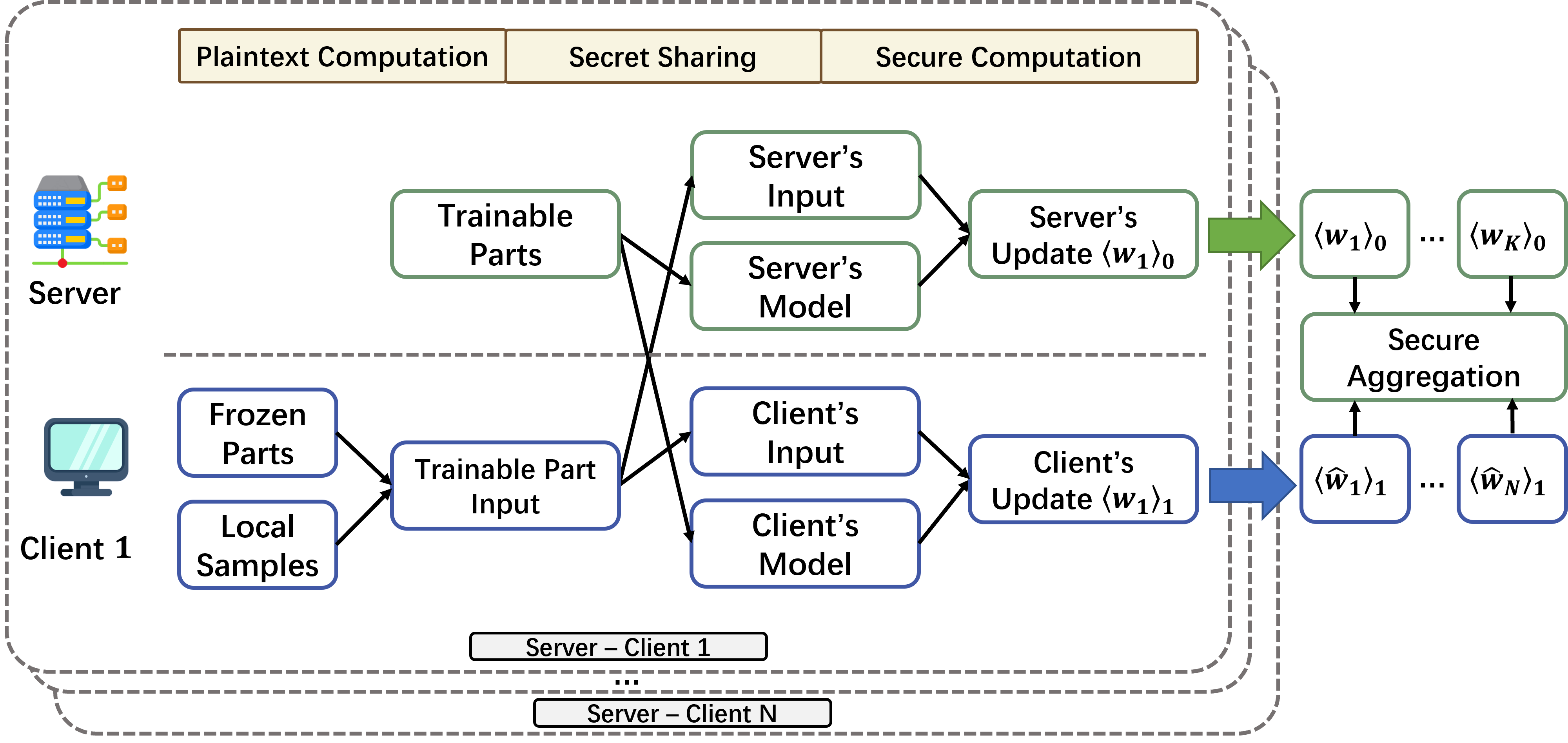
Figure 2: A simple illustration of PriFFT framework.

Fig. 2 presents the framework of PriFFT. There are $N$ clients participating in FL training. For each client $i$, the training data is presented as $(x_{i},y_{i})$, where $x_{i}$ and $y_{i}$ are training samples and labels. The model structure and parameters are $f$ and $\omega$, respectively. Parameters are divided into the frozen part $\omega_{\mathbf{F}}$ and the trainable part $\omega_{\mathbf{T}}$, where $\omega=\omega_{\mathbf{F}}\cup\omega_{\mathbf{T}}$. The frozen part $\omega_{\mathbf{F}}$ remains constant, and the trainable part $\omega_{\mathbf{T}}$ is adjusted by clients’ data through local training.

The trainable model parameters $\omega_{\mathbf{T}}$ are transmitted to clients in the form of shares. The number of training rounds is $T$. In the $t$-th ($t\in\left[1,\cdots,T\right]$) training round, the server splits the latest trainable parameters $\omega_{\mathbf{T},t}$ into $\left\langle\omega_{\mathbf{T},t}\right\rangle_{b}$ ($b\in\{0,1\}$) where $\omega_{\mathbf{T},t}=\left\langle\omega_{\mathbf{T},t}\right\rangle_{0}+\left\langle\omega_{\mathbf{T},t}\right\rangle_{1}$. Similarly, client $i$ randomly samples and splits a batch of sample $(x_{i},y_{i})$ such that $x_{i}=\left\langle x_{i}\right\rangle_{0}+\left\langle x_{i}\right\rangle_{1}$ and $y_{i}=\left\langle y_{i}\right\rangle_{0}+\left\langle y_{i}\right\rangle_{1}$. The sever and client $i$ exchange shares of model parameters and sample data so that the server gets $\{\left\langle\omega_{\mathbf{T},t}\right\rangle_{0},\left\langle x_{i}\right\rangle_{0},\left\langle y_{i}\right\rangle_{0}\}$ and client $i$ gets $\{\left\langle\omega_{\mathbf{T},t}\right\rangle_{1},\left\langle x_{i}\right\rangle_{1},\left\langle y_{i}\right\rangle_{1}\}$. Model parameters in the $t$-training round are $\omega_{t}=\omega_{\mathbf{F}}\cup\omega_{\mathbf{T},t}$. Since PriFFT splits $\omega_{\mathbf{T},t}$ into two shares, the protected model parameters are represented by $\hat{\omega}_{b,t}=\omega_{\mathbf{F}}\cup\left\langle\omega_{\mathbf{T},t}\right\rangle_{b}$ where $b\in\{0,1\}$.

PriTFF transfers $f_{\mathbf{T}}$ to $\hat{f}_{\mathbf{T}}$ by our designed secure computation protocols such that $f(x_{i};\omega_{t})=\hat{f}(\left\langle x_{i}\right\rangle_{0};\hat{\omega}_{0,t})+\hat{f}(\left\langle x_{i}\right\rangle_{1};\hat{\omega}_{1,t})$. Similarly, PriTFF transfers the loss function $L$ to $\hat{L}$ and presents secure gradient computation method such that $L(f(x_{i};w_{t}),y_{i})=\hat{L}(\hat{f}(\left\langle x_{i}\right\rangle_{0};\hat{\omega}_{0,t}),\left\langle y_{i}\right\rangle_{0})+\hat{L}(\hat{f}(\left\langle x_{i}\right\rangle_{1};\hat{\omega}_{1,t}),\left\langle y_{i}\right\rangle_{1})$ and

$$\frac{\partial L(f(x_{i};w_{t}),y_{i})}{\partial\omega_{\mathbf{T},t}}=\sum_{b\in\{0,1\}}\frac{\hat{L}(\hat{f}(\left\langle x_{i}\right\rangle_{b};\hat{\omega}_{b,t}),\left\langle y_{i}\right\rangle_{b})}{\partial\left\langle\omega_{\mathbf{T},t}\right\rangle_{b}}.$$ (1)

We use $\left\langle g_{i,t}\right\rangle_{b}$ to represent the protected gradients of trainable parameters in the right term of Equation (1). In other words, $\left\langle g_{i,t}\right\rangle_{b}$ is the share of the trainable parameter gradients generated by client $i$’s samples in the $t$-th training round. Similarly, the left term of Equation (1) is presented by $g_{i,t}$. In the aggregation phase of the $t$-th training round, the server needs to calculate the aggregated gradients by

$$\bar{g}_{t}=\frac{1}{N}\sum_{i=1}^{N}g_{i,t}=\frac{1}{N}\sum_{i=1}^{N}\left(\left\langle g_{i,t}\right\rangle_{0}+\left\langle g_{i,t}\right\rangle_{1}\right).$$ (2)

The server can directly get $\left\langle g_{i,t}\right\rangle_{1}$ by $\sum_{b\in\{0,1\}}\left\langle g_{i,t}\right\rangle_{b}$ if client $i$ uploads $\left\langle g_{i,t}\right\rangle_{1}$ to the server, leading to privacy leakage of clients’ training samples due to reconstruction attacks against gradients. We apply the secure aggregation [26] to protect $\left\langle g_{i,t}\right\rangle_{b}$. Specifically, client $i$ masks shared gradients $\left\langle g_{i,t}\right\rangle_{1}$ to double masked gradients $[\![g_{i,t}]\!]_{1}$ such that

$$\left\{\begin{matrix}g_{i,t}\neq\left\langle g_{i,t}\right\rangle_{0}+[\![g_{i,t}]\!]_{1};\\ \bar{g}_{t}=\frac{1}{N}\sum_{i=1}^{N}g_{i,t}=\frac{1}{N}\sum_{i=1}^{N}\left(\left\langle g_{i,t}\right\rangle_{0}+[\![g_{i,t}]\!]_{1}\right).\end{matrix}\right.$$ (3)

In other words, the server cannot restore $g_{i,t}$ by $[\![g_{i,t}]\!]_{1}$ but still get the correct aggregated gradients $\bar{g}_{t}$ by the sum of gradients from the server and clients.

The process of the $t$-th training round can be summarized as: (i) the server and client $i$ send $\hat{\omega}_{1,t}$ and $\{\left\langle x_{i}\right\rangle_{0},\left\langle y_{i}\right\rangle_{0}\}$ to each other, restively; (ii) the server and client $i$ compute $\left\langle g_{i,t}\right\rangle_{b}$ via presented secure computation protocols; (iii) client $i$ masks $\left\langle g_{i,t}\right\rangle_{1}$ to $[\![g_{i,t}]\!]_{1}$ and uploads $[\![g_{i,t}]\!]_{1}$ to the server; (iv) the server calculates aggregated gradients $\bar{g}_{t}$ and optimizes the model parameters. The above process occurs in parallel between the server and each client.

V Secure Computation Protocols for PriFFT

V-A Multiplication and Truncation

V-A1 Matrix Multiplication

Matrix multiplication is a fundamental calculation in fine-tuning of LLMs, which implements the fully connected layers and convolutional layers. PriFFT implements matrix multiplication based on the arithmetic secret sharing in Section III-B. Specifically, given matrix $X\in\mathbb{Z}_{2^{l}}^{u\times v}$, $Y\in\mathbb{Z}_{2^{l}}^{v\times w}$ and shares $\left\langle X\right\rangle_{b}$, $\left\langle Y\right\rangle_{b}$, computing $\left\langle X\cdot Y\right\rangle_{b}$ requires generating corresponding dimension Beaver triples $\{C\in\mathbb{Z}_{2^{l}}^{u\times w},A\in\mathbb{Z}_{2^{l}}^{u\times v},B\in\mathbb{Z}_{2^{l}}^{v\times w}\}$ in the offline phase such that $\left\langle C\right\rangle_{b}=\left\langle A\cdot B\right\rangle_{b}$. When party $P_{b}$ computes $\left\langle X\cdot Y\right\rangle_{b}$, $P_{b}$ sets $\left\langle E\right\rangle_{b}=\left\langle X\right\rangle_{b}-\left\langle A\right\rangle_{b}$ and $\left\langle F\right\rangle_{b}=\left\langle Y\right\rangle_{b}-\left\langle B\right\rangle_{b}$. Both parties restore $E$ and $F$ by exchanging corresponding shares. Parties $P_{b}$ computes $\left\langle X\cdot Y\right\rangle_{b}=b\cdot E\cdot F+\left\langle A\right\rangle_{b}\cdot F+E\cdot\left\langle B\right\rangle_{b}+\left\langle C\right\rangle_{b}).$ The communication happens on exchanging $\{\left\langle E\right\rangle_{b},\left\langle F\right\rangle_{b}\}$, and the communication overhead is $\left(2luv+2lvs\right)$ bits

V-A2 Truncation

The scale of multiplication results between shared values would become $2^{2s}$. The truncation $\mathrm{Trunc}(\left\langle x\right\rangle_{b},s)$ reduces the scale from $2^{2s}$ to $2^{s}$. A straightforward implementation is local truncations (LT), i.e., each party directly divides $\left\langle x\right\rangle_{b}$ by $2^{s}$. LT produces results with errors when the sum of shares wraps around the ring size. We introduce the truncation method proposed in CRYPTEN [35] as interactive truncations (IT). $\mathrm{Trunc}(\left\langle x\right\rangle_{b},s)$ with IT invokes the communication of $l$ bits in the online phase. Evaluation results in Section VII-B show that the difference in accuracy between models fine-tuning with IT and LT is insignificant. We propose to reduce the communication overhead in the early stages of fine-tuning with LT. When the model tends to converge, fine-tuning with IT is applied to improve the model accuracy further. Unless otherwise specified, the communication overhead discussed in Section V does not include the truncation cost since we consider two truncation methods.

V-A3 Power Functions

Since several computations in PriFFT involve the secure square function, we present a secure square function based on offset functions of FSS to reduce the communication overhead. The straightforward way to implement the square function is using ASS multiplication given in Section III-B. The communication overhead of computing $x^{2}$ for a value $x\in\mathbb{Z}_{2^{l}}$ is $4l$ bits. The proposed secure square function with FSS reduces communication overhead from $4l$ bits to $2l$ bits. We leave the construction detail of the secure square function in APPENDIX B-B. Similar to the construction of $\mathrm{Gen}^{\mathrm{square}}_{l}$ and $\mathrm{Eval}^{\mathrm{square}}_{l,l}$, we present $\mathrm{Gen}^{\mathrm{mul}}_{l,l}$ and $\mathrm{Eval}^{\mathrm{mul}}_{l,l}$ to implement multiplications with FSS, while the construction detail is given in Appendix B-A. Besides, it is straightforward to construct the secure power function, which is similar to the construction of the secure square function. Due to the space limitation, we leave the construction details to APPENDIX B-B.

V-B Natural Exponential Function

Existing works perform secure interval estimation of the input $x$ and approximate the results through secure linear computations. For example, as shown in Fig. 3, Boyle et al. present spline functions based on FSS to deal with non-linear computations [36], in which interval estimation involves multiple secure comparisons of $x$. Enhancing interval evaluation accuracy improves the precision of secure computation results, but it also necessitates more secure comparisons. Secure comparisons incur a higher computation overhead than secure linear computations. Therefore, we consider iterative methods that approximate $e^{x}$ with the linear computations.

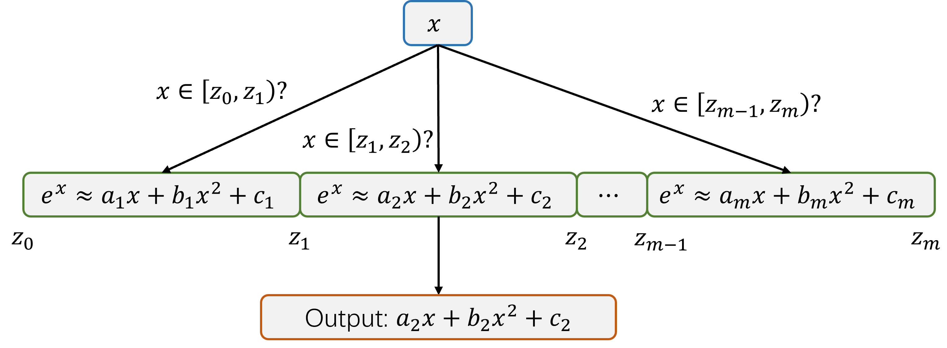
Figure 3: An example of approximating $e^{x}$ by spline functions.

Our approximation comes from the limit definition of the natural exponential function $e^{x}=\lim_{n\rightarrow\infty}\left(1+x/n\right)^{n}$. We approximate the shares of $e^{x}$ from the shares of $x$ by $\left\langle e^{x}\right\rangle_{b}=\left(1+\left\langle x\right\rangle_{b}/n\right)^{n}$. Assume that $n=2^{m}$, we have

$$\left(1+\frac{x}{n}\right)^{n}=\left(1+\frac{x}{2^{m}}\right)^{2^{m}}=\left[\left(1+\frac{x}{2^{m}}\right)^{2}\right]^{2^{m-1}}.$$ (4)

In other words, performing $m$ squares for $\left(1+x/2^{m}\right)$ and its subsequent results yields the result of $\left(1+x/n\right)^{n}$ where $n=2^{m}$. For a share $\left\langle x\right\rangle_{b}\in\mathbb{Z}_{2^{l}}$ of $x$, the computation in Equation (4) involves a truncation to compute $\left(1+x/2^{m}\right)$ and $m$ secure square functions. We define the natural exponential function gate $\mathcal{G}_{\mathrm{exp}}$ as the family of functions $g_{\mathrm{exp},l}:\mathbb{Z}_{2^{l}}\rightarrow\mathbb{Z}_{2^{l}}$ with input group $\mathbb{G}^{\mathrm{in}}=\mathbb{Z}_{2^{l}}$, output group $\mathbb{G}^{\mathrm{out}}=\mathbb{Z}_{2^{l}}$, and $g_{\mathrm{exp},l}(x):=e^{x}$. Using Equation (4) to approximate $e^{x}$, we denote the natural exponential function gate with FSS by $\hat{\mathcal{G}}_{\mathrm{exp}}$ and the offset functions by:

$$\hat{g}_{\mathrm{exp},l}^{\left[r^{\mathrm{in}},r^{\mathrm{out}}\right]}(\hat{x}) =g_{\mathrm{exp},l}(\hat{x}-r^{\mathrm{in}})+r^{\mathrm{out}}\mod 2^{l}$$

$$=\left(1+\frac{\hat{x}-r^{\mathrm{in}}}{2^{m_{\exp}}}\right)^{2^{m_{\exp}}}+r^{\mathrm{out}}\mod 2^{l},$$ (5)

where $m_{\exp}$ is the number of approximation iterations.

1 Requires: Input offset $r^{\text{in}}$, output offset $r^{\text{out}}$, iteration rounds $m_{\exp}$, intermediate offsets $\mathbf{r}=\{r^{(1)},\cdots,r^{(m_{\exp})}\}$.

2 Output: Evaluation keys $(k_{0},k_{1})$.

3 Sample random $r^{\text{in}}_{0}$, $r^{\text{in}}_{1}$, $r^{\text{out}}_{0}$, $r^{\text{out}}_{1}\in\mathbb{Z}_{2^{l}}$, s.t., $r^{\text{in}}_{0}+r^{\text{in}}_{1}=r^{\text{in}}\mod 2^{l}$, $r^{\text{out}}_{0}+r^{\text{out}}_{1}=r^{\text{out}}\mod 2^{l}$;

4 foreach $r_{i}\in\{r^{(1)},\cdots r^{({m_{\exp}})}\}$ do

5    Sample random $r^{(i)}_{0}$, $r^{(i)}_{1}$, $q^{(i)}_{0}$, $q^{(i)}_{1}\in\mathbb{Z}_{2^{l}}$, s.t., $r^{(i)}_{0}+r^{(i)}_{1}=r^{(i)}\mod 2^{l}$, $q^{(i)}_{0}+q^{(i)}_{1}=\left[r^{(i)}\right]^{2}\mod 2^{l}$;

6   

7For $b\in\{0,1\}$, let $k_{b}=r^{\text{in}}_{b}\|r^{(1)}_{b}\|q^{(1)}_{b}\|\cdots\|r^{(m_{\exp})}_{b}\|q^{(m_{\exp})}_{b}\|r^{\text{out}}_{b}$;

return $(k_{0},k_{1})$

Algorithm 1 Natural exponential function ($e^{x}$) with FSS in the offline stage $\mathrm{Gen}^{\mathrm{exp}}_{l}(r^{\text{in}},r^{\text{out}},\mathbf{r})$

We present the offline stage of the natural exponential function gate with FSS in Algorithm 1. The implementation computes $(1+\hat{x}/2^{m_{\exp}})$ locally and then performs $m_{\exp}$ times square functions with FSS. We introduce additional offsets $\left\{r^{(1)}\cdot,r^{(m_{\exp})}\right\}$ to protect the intermediate results of square functions. The key generation only shares $r^{(i)}$ and $\left[r^{(i)}\right]^{2}$ instead of directly applying $m_{\exp}$ times $\mathrm{Gen}^{\mathrm{square}}_{l}(r^{(i)},r^{(i+1)})$.

Algorithm 2 presents the online stage of the natural exponential function with FSS. We first compute $\left(1+x/2^{m_{\exp}}\right)$ by the masked input $\hat{x}$ (line 6). The term $2^{s}b$ refers to 1 on the ring $\mathbb{Z}_{2^{l}}$ in the above equation. The value of $x/2^{m_{\exp}}$ is computed by a truncation function $\mathrm{Trunc}(\hat{x}-r^{\text{in}}_{b},m_{\exp})$. The intermediate result $t^{(i)}_{b}$ is masked by off offset $r_{b}^{(1)}$. In each square computation, both parties compute the square results with corresponding offsets (line 13).

1 Requires: Evaluation keys $(k_{0},k_{1})$, additive shares $(\left\langle\hat{x}\right\rangle_{0},\left\langle\hat{x}\right\rangle_{1})$ of $\hat{x}$ with offset $r^{\text{in}}$, scale factor $s$.

2 Output: Shares of $e^{\hat{x}-r^{\text{in}}}+r^{\text{out}}$.

3 Restore $\hat{x}=x+r^{\mathrm{in}}$ from shares of $\hat{x}$;

4 for $b\in\{0,1\}$ do

5    Parse $k_{b}=r^{\text{in}}_{b}\|r^{(1)}_{b}\|q^{(1)}_{b}\|\cdots\|r^{(m_{\exp})}_{b}\|q^{(m_{\exp})}_{b}\|r^{\text{out}}_{b}$;

6    $\left\langle\hat{t}_{0}\right\rangle_{b}=\mathrm{Trunc}(\hat{x}-r^{\text{in}}_{b},m_{\exp})+2^{s}b+r^{(1)}_{b}\mod 2^{l}$;

7for $i=1\>\mathrm{to}\>m_{\exp}$ do

8    for $b\in\{0,1\}$ do

9       if $i<m_{\exp}$ then

10          $k_{b}^{\mathrm{square}}=r^{(i)}_{b}\|q^{(i)}_{b}\|r^{(i+1)}_{b}$ ;

11         

12      else

13          $k_{b}^{\mathrm{square}}=r^{(i)}_{b}\|q^{(i)}_{b}\|r^{\text{out}}_{b}$ ;

14      $\left\langle\hat{t}_{i}\right\rangle_{b}=\mathrm{Eval}^{\mathrm{square}}_{l}(b,k_{b}^{\mathrm{square}},\left\langle\hat{t}_{i-1}\right\rangle_{b})$

15      

16   

return $(\left\langle\hat{t}_{m_{\exp}}\right\rangle_{0},\left\langle\hat{t}_{m_{\exp}}\right\rangle_{1})$

Algorithm 2 Natural exponential function ($e^{x}$) with FSS in the online stage $\mathrm{Eval}^{\mathrm{exp}}_{l}(b,k_{b},\left\langle\hat{x}\right\rangle_{b})$

The communication overhead of the natural exponential function gate with FSS is $2l\cdot(m_{\exp}+1)$ bits, which results from the restoration of intermediate values. When using ASS to approximate the natural exponential function, the communication overhead is $4ml$ bits where $(1+x/2^{m_{\exp}})$ is computed locally, and each restore of square results cost $4l$ bits.

V-C Softmax and Hyperbolic Tangent

The softmax function takes a vector $\mathbf{z}=\left\{z_{1},z_{2},\cdots,z_{K}\right\}$ as input and normalizes $\mathbf{z}$ into a probability distribution consisting of $K$ probabilities, i.e., the softmax function rescales $\mathbf{z}$ so that the output lies in the range $\left[0,1\right]$ and sums to $1$. The softmax function is given by $\mathrm{Softmax}(\mathbf{z})_{i}=e^{z_{i}}/\sum_{j=1}^{K}e^{z_{j}}$. The hyperbolic tangent function is a popular activation function in neural networks, which is given by $\mathrm{Tanh}(x)=(e^{2x}-1)/(e^{2x}+1)$.

The softmax and hyperbolic tangent functions involve natural exponential functions and division. We have discussed the implementation of natural exponential functions in Section V-B. The division between two FSS shares is given as follows. We approximate the reciprocal of a divisor using Newton’s method by setting $f(x)=(1/x-a)$ and

$$x_{n+1}=x_{n}-\frac{f(x_{n})}{f^{\prime}(x_{n})}=x_{n}-\frac{\frac{1}{x_{n}}-a}{\frac{1}{x^{2}_{n}}}=x_{n}(2-ax_{n}),$$ (6)

where $a$ is the input. Our evaluation results show that the correct result can only be obtained when the sign of $x_{0}$ is the same as that of the divisor. Therefore, we set $x_{0}\in\mathbb{Z}_{2l}^{+}$ to be a positive value and then apply the secure computation discussed in Section III-C to ensure the sign of $x_{0}$ with that of the divisor.

We define the reciprocal gate $\mathcal{G}_{\mathrm{recip}}$ as the family of functions $g_{\mathrm{recip},l}:\mathbb{Z}_{2^{l}}\rightarrow\mathbb{Z}_{2^{l}}$ with input group $\mathbb{G}^{\mathrm{in}}=\mathbb{Z}_{2^{l}}$, output group $\mathbb{G}^{\mathrm{out}}=\mathbb{Z}_{2^{l}}$, and $g_{\mathrm{recip},l}(x):=1/x$. Using Newton’s method to approximate $1/x$, we denote the reciprocal gate with FSS by $\hat{\mathcal{G}}_{\mathrm{recip}}$ and the offset functions by:

$$\hat{g}_{\mathrm{recip},l}^{\left[r^{\mathrm{in}},r^{\mathrm{out}}\right]}(\hat{x}) =g_{\mathrm{recip},l}(\hat{x}-r^{\mathrm{in}})+r^{\mathrm{out}}\mod 2^{l}$$

$$=h_{m}+r^{\mathrm{out}}\mod 2^{l}$$ (7)

where

$$h_{i}=\left\{\begin{matrix}x^{\prime}_{0}\cdot\left[2-(\hat{x}-r^{\mathrm{in}})\cdot x^{\prime}_{0}\right]\mod 2^{l},\;&\mathrm{if}\;i=0;\\ h_{i-1}\cdot\left[2-(\hat{x}-r^{(i)})\cdot h_{i-1}\right]\mod 2^{l},\;&\mathrm{else},\end{matrix}\right.$$ (8)

$x^{\prime}_{0}=x_{0}\cdot(1-2\cdot\mathbf{1}\{\hat{x}<r^{\mathrm{in}}\})$, $m$ is the iteration round, and $r^{(i)}$ is the intermediate mask.

Algorithm 3 presents the offline stage of the reciprocal operation with FSS. The key generation of reciprocal operation is similar to that of the natural exponential function. The difference is Algorithm 3 applies $\mathrm{Gen}^{<}_{l}$ to generate the comparison keys such that $\mathrm{Eval}^{<}_{l}$ outputs $1$ when the input $\hat{x}<r^{\mathrm{in}}$ (line 3). Besides, Algorithm 3 generates shares of offsets to support multiplications with FSS (line 7).

1 Requires: Input offset $r^{\text{in}}$, output offset $r^{\text{out}}$, iteration rounds $m_{\mathrm{recip}}$, intermediate offsets $\mathbf{r}=\{r^{(1)},\cdots,r^{(2m_{\mathrm{recip}})}\}$, security parameter $\lambda$.

2 Output: Evaluation keys $(k_{0},k_{1})$.

3 $(c_{0},c_{1})\leftarrow\mathrm{Gen}^{<}_{l}(1^{\lambda},r^{\mathrm{in}},1,\mathbb{Z}_{2^{l}});$

4 Sample random $r^{\text{in}}_{0}$, $r^{\text{in}}_{1}$, $r^{\text{out}}_{0}$, $r^{\text{out}}_{1}\in\mathbb{Z}_{2^{l}}$, s.t., $r^{\text{in}}_{0}+r^{\text{in}}_{1}=r^{\text{in}}\mod 2^{l}$, $r^{\text{out}}_{0}+r^{\text{out}}_{1}=r^{\text{out}}\mod 2^{l}$;

5 foreach $i\in\{1,\cdots,m_{\mathrm{recip}}\}$ do

6    Sample random $r^{(i)}_{0}$, $r^{(i)}_{1}$, $q^{(i)}_{0}$, $q^{(i)}_{1}$, s.t., $r^{(i)}_{0}+r^{(i)}_{1}=r^{(2i-1)}\mod 2^{l}$, $q^{(i)}_{0}+q^{(i)}_{1}=\left[r^{(2i-1)}\right]^{2}\mod 2^{l}$;

7    Sample random $u^{(i)}_{0}$, $u^{(i)}_{1}$, $v^{(i)}_{0}$, $v^{(i)}_{1}$, s.t., $u^{(i)}_{0}+u^{(i)}_{1}=r^{(2i)}\mod 2^{l}$, $v^{(i)}_{0}+v^{(i)}_{1}=r^{(2i)}r^{\mathrm{in}}\mod 2^{l}$;

8   

9For $b\in\{0,1\}$, let $k_{b}=c_{b}\|r^{\text{in}}_{b}\|r^{(1)}_{b}\|q^{(1)}_{b}\|u^{(1)}_{b}\|v^{(1)}_{b}\|\cdots\|v^{(m_{\mathrm{recip}})}_{b}\|r^{\text{out}}_{b}$;

return $(k_{0},k_{1})$

Algorithm 3 Reciprocal ($1/x$) with FSS in the offline stage $\mathrm{Gen}^{\mathrm{recip}}_{l}(\lambda,r^{\text{in}},r^{\text{out}},\mathbf{r})$

Algorithm 4 presents the online stage of the reciprocal operation with FSS. Algorithm 4 firstly adjust the sign of initial guess $x_{0}$ based on secure comparison (line 6). The comparison result of $\hat{x}<r^{\mathrm{in}}$ equals the result of $x<0$ since $\hat{x}=x+r^{\mathrm{in}}$. The adjusted initial guess is masked by the offset $r_{b}^{(1)}$ to support the implementation with FSS. The approximation of the reciprocal is obtained through the iteration of Equation (6) (lines 7-16). We compute $x_{n}^{2}$ by the FSS square gate (line 14) and $ax_{n}^{2}$ by the FSS multiplication gate (line 15). The intermediate result in each iteration $\hat{t}_{b}^{(i)}$ is $2x_{n}-ax_{n}^{2}$ (line 16), where $\hat{t}^{(i-1)}_{b}-r^{(i-1)}_{b}$ removes the offset of $\hat{t}^{(i-1)}_{b}$ so that the offset of $\hat{t}_{b}^{(i)}$ is $r^{(i-1)}_{b}$ or $r^{\mathrm{out}}_{b}$.

1 Requires: Evaluation keys $(k_{0},k_{1})$, additive shares $(\left\langle\hat{x}\right\rangle_{0},\left\langle\hat{x}\right\rangle_{1})$ of $\hat{x}$ with offset $r^{\text{in}}$, initial guess $x_{0}$.

2 Output: Shares of $\frac{1}{\hat{x}-r^{\mathrm{in}}}+r^{\text{out}}$.

3 Restore $\hat{x}=x+r^{\mathrm{in}}$ from shares of $\hat{x}$;

4 for $b\in\{0,1\}$ do

5    Parse $k_{b}=c_{b}\|r^{\text{in}}_{b}\|r^{(1)}_{b}\|q^{(1)}_{b}\|u^{(1)}_{b}\|v^{(1)}_{b}\|\cdots\|v^{(m_{\mathrm{recip}})}_{b}\|r^{\text{out}}_{b}$

6    $\left\langle\hat{t}_{0}\right\rangle_{b}=x_{0}\cdot\left[1-2\cdot\mathrm{Eval}^{<}_{l}(b,c_{b},\hat{x})\right]+r_{b}^{(1)}$;

7   

8for $i=1\>\mathrm{to}\>m_{\mathrm{recip}}$ do

9    for $b\in\{0,1\}$ do

10       $k_{b}^{\mathrm{square}}=r^{(i)}_{b}\|q^{(i)}_{b}\|u_{b}^{(i)}$ ;

11       if $i<m_{\mathrm{recip}}$ then

12          $k_{b}^{\mathrm{mul}}=r_{b}^{\mathrm{in}}\|u_{b}^{(i)}\|v_{b}^{(i)}\|r^{(i+1)}_{b}$ ;

13         

14      else

15          $k_{b}^{\mathrm{mul}}=r_{b}^{\mathrm{in}}\|u_{b}^{(i)}\|v_{b}^{(i)}\|r^{\mathrm{out}}_{b}$ ;

16         

17      $\left\langle\hat{t}_{i}\right\rangle_{b}=\mathrm{Eval}^{\mathrm{square}}_{l}(b,k_{b}^{\mathrm{square}},\left\langle\hat{t}_{i-1}\right\rangle_{b})$;

18       $\left\langle\hat{t}_{i}\right\rangle_{b}=\mathrm{Eval}^{\mathrm{mul}}_{l,l}(b,k_{b}^{\mathrm{mul}},\hat{x},\left\langle\hat{t}_{i}\right\rangle_{b})$;

19       $\left\langle\hat{t}_{i}\right\rangle_{b}=2\cdot\left[\left\langle\hat{t}_{i-1}\right\rangle_{b}-r^{(i-1)}_{b}\right]-\left\langle\hat{t}_{i}\right\rangle_{b}\mod 2^{l};$

20      

21   

return $(\left\langle\hat{t}_{m_{\mathrm{recip}}}\right\rangle_{0},\left\langle\hat{t}_{m_{\mathrm{recip}}}\right\rangle_{1})$

Algorithm 4 Reciprocal ($1/x$) with FSS in the online stage $\mathrm{Eval}^{\mathrm{recip}}_{l}(b,k_{b},\left\langle\hat{x}\right\rangle_{b})$

We implement the secure $\mathrm{Softmax}(x)$ and $\mathrm{Tanh}(x)$ by combining the secure $e^{x}$, reciprocal calculation and multiplication. Due to the space limitation, the detailed construction of the above two protocols is given in Appendix B-C.

V-D Dropout

During the training process, the dropout operation randomly zeroes some of the input elements with probability $p$. Furthermore, the outputs are scaled by a factor of $\frac{1}{1-p}$. For convenience, we define the dropout function by

$$\mathrm{Dropout}(x;p)=\left\{\begin{matrix}0,\;&\mathrm{with\;probability}\;p;\\ \frac{x}{1-p},\;&\mathrm{else}.\end{matrix}\right.$$ (9)

We define the dropout gate $\mathcal{G}_{\mathrm{drop}}$ as the family of functions $g_{\mathrm{drop},l}:\mathbb{Z}_{2^{l}}\rightarrow\mathbb{Z}_{2^{l}}$ with input $\mathbb{G}^{\mathrm{in}}=\mathbb{Z}_{2^{l}}$, output $\mathbb{G}^{\mathrm{out}}=\mathbb{Z}_{2^{l}}$, and $g_{\mathrm{drop},l}(x;p):=\mathrm{Dropout}(x;p)$. We denote the dropout gate with FSS by $\hat{\mathcal{G}}_{\mathrm{drop}}$ and the offset functions by:

$$\hat{g}_{\mathrm{drop},l}^{\left[r^{\mathrm{in}},r^{\mathrm{out}}\right]}(\hat{x}) =g_{\mathrm{drop},l}(\hat{x}-r^{\mathrm{in}})+r^{\mathrm{out}}\mod 2^{l}$$

$$=\frac{\hat{x}-r^{\mathrm{in}}}{1-p}\cdot\mathbf{1}\{r<p\}$$ (10)

where $r\in(0,1)$ is a random number. The straightforward way to implement a dropout gate is to generate random numbers belonging to the interval $(0,1)$ during the offline stage and then apply secure comparison to compare these random numbers with $p$ during the online stage. However, the key of the dropout function is to calculate $\sigma=\mathbf{1}\{r<p\}/(1-p)$. Obviously, the comparison can be done during the offline stage, and the results of $\sigma$ can be saved as keys to avoid the comparison operation during the online stage.

Based on the above analysis, we present the offline stage of the dropout gate with FSS in algorithm 5. The algorithm first samples random numbers $r\in(0,1)$ for comparison (line 3). The dropout factor $\sigma$ is determined by the comparison result $\mathbf{1}\{r<p\}$ and the dropout probability $p$ (line 4). We split the offsets (line 5) and mask $\sigma$ by $r^{\sigma}$ (line 6) so that each party cannot learn $\sigma$ from keys. Algorithm 6 presents the online stage of the dropout function. The main idea of the algorithm is to realize the multiplication of the dropout factor $\hat{\sigma}$ and the input $\hat{x}$ through $\mathrm{Eval}_{l,l}^{\mathrm{mul}}$. Since $\hat{\sigma}$ is embedded into the keys during the offline stage, the evaluation omits the restoration of $\hat{\sigma}$ and reduces communication overhead.

1 Requires: Input offset $r^{\text{in}}$, output offset $r^{\text{out}}$, factor offset $r^{\sigma}$, dropout probability $p$.

2 Output: Evaluation keys $(k_{0},k_{1})$.

3 Sample random $r\in(0,1)$;

4 $\sigma=\frac{1}{1-p}\cdot\mathbf{1}\{r<p\}$ ;

5 $\hat{\sigma}=\sigma+r^{\sigma}$;

6 $k_{b}^{\mathrm{mul}}=\mathrm{Gen}_{l,l}^{\mathrm{mul}}(r^{\mathrm{in}},r^{\mathrm{\sigma}},r^{\mathrm{out}})$;

7 For $b\in\{0,1\}$, let $k_{b}=k_{b}^{\mathrm{mul}}\|\hat{\sigma}$ ;

return $(k_{0},k_{1})$

Algorithm 5 Dropout function with FSS in the offline stage $\mathrm{Gen}^{\mathrm{drop}}_{l}(r^{\text{in}},r^{\text{out}},r^{\sigma},p)$

1 Requires: Evaluation keys $(k_{0},k_{1})$, additive shares $(\left\langle\hat{x}\right\rangle_{0},\left\langle\hat{x}\right\rangle_{1})$ of $\hat{x}$ with offset $r^{\text{in}}$, scale factor $s$.

2 Output: Shares of $\mathrm{Dropout}(\hat{x}-x^{\mathrm{in}})+r^{\text{out}}$.

3 for $b\in\{0,1\}$ do

4    Parse $k_{b}=k_{b}^{\mathrm{mul}}\|\hat{\sigma}$;

5    Parse $k_{b}^{\mathrm{mul}}=r^{\text{in}_{1}}_{b}\|r^{\text{in}_{2}}_{b}\|q_{b}\|r^{\text{out}}_{b}$;

6    Restore $\hat{x}=x+r^{\mathrm{in}_{1}}$ from shares of $\hat{x}$ ;

7    $t_{b}=\mathrm{Trunc}(b\hat{x}\hat{\sigma}-\hat{x}r^{\mathrm{in}_{2}}_{b}-\hat{\sigma}r^{\mathrm{in}_{1}}_{b}+q_{b},s)+r^{\text{out}}_{b}\mod 2^{l}$;

8   

return $(\left\langle\hat{t}\right\rangle_{0},\left\langle\hat{t}\right\rangle_{1})$

Algorithm 6 Dropout function with FSS in the online stage $\mathrm{Eval}^{\mathrm{drop}}_{l}(b,k_{b},\left\langle\hat{x}\right\rangle_{b})$

We refer to the above dropout method, which completes random number comparison in the offline stage, as the static dropout. A shortcoming is that the dropout probability must stay the same in secure federated fine-tuning. Therefore, we also consider the dynamic dropout in the evaluation, in which the key holds random values in the offline stage. The secure comparison calculates the dropout factor according to the random values and dynamic probability in the online stage.

V-E Tensor Product of Vectors

We consider the vectors $\mathbf{v}=\{v_{1},v_{2},\cdots,v_{n}\}$ and $\mathbf{w}=\{w_{1},w_{2},\cdots,w_{m}\}$ to discuss the tensor product of vectors. The tensor product $\mathbf{v}\otimes\mathbf{w}$ generates a $n\times m$ matrix such that

$$\mathbf{v}\otimes\mathbf{w}=\left(\begin{array}[]{cccc}v_{1}w_{1}&v_{1}w_{2}&\cdots&v_{1}w_{m}\\ v_{2}w_{1}&v_{2}w_{2}&\cdots&v_{2}w_{m}\\ \vdots&\vdots&\ddots&\vdots\\ v_{n}w_{1}&v_{n}w_{2}&\cdots&v_{n}w_{m}\end{array}\right).$$ (11)

The backpropagation of the model involves the tensor product of vectors, in which the linear layer gradient calculation involves the tensor product of the parameters and the gradients of the next layer. A straightforward way to implement the tensor product of vectors is to treat $\mathbf{v}$ and $\mathbf{w}$ as $n\times 1$ and $1\times m$ matrices and obtain $\mathbf{v}\otimes\mathbf{w}$ through matrix multiplication. The key size of the above matrix multiplication is $3lmn$ bits, while the communication overhead is $\left(2lm+2ln\right)$ bits.

1Requires: Input offsets $\{\mathbf{r}^{\text{in}_{1}},\mathbf{r}^{\text{in}_{2}}\}$, output offset $\mathbf{r}^{\text{out}}$.

2 Output: Evaluation keys $(k_{0},k_{1})$.

3 Sample random $\mathbf{r}^{\text{in}_{1}}_{0}$, $\mathbf{r}^{\text{in}_{1}}_{1}\in\mathbb{Z}_{2^{l}}^{N}$, $\mathbf{r}^{\text{in}_{2}}_{0}$, $\mathbf{r}^{\text{in}_{2}}_{1}\in\mathbb{Z}_{2^{l}}^{M}$, $\mathbf{r}^{\text{out}}_{0}$, $\mathbf{r}^{\text{out}}_{1}\in\mathbb{Z}_{2^{l}}^{N\times M}$, s.t., $\mathbf{r}^{\text{in}_{1}}_{0}+\mathbf{r}^{\text{in}_{1}}_{1}=\mathbf{r}^{\text{in}_{1}}\mod 2^{l}$, $\mathbf{r}^{\text{in}_{2}}_{0}+\mathbf{r}^{\text{in}_{2}}_{1}=\mathbf{r}^{\text{in}_{2}}\mod 2^{l}$, $\mathbf{r}^{\text{out}}_{0}+\mathbf{r}^{\text{out}}_{1}=\mathbf{r}^{\text{out}}\mod 2^{l}$;

4 Sample random $\mathbf{q}_{0},\mathbf{q}_{1},\in\mathbb{Z}_{2^{l}}^{N\times M}$, s.t., $\mathbf{q}_{0}+\mathbf{q}_{1}=\mathbf{r}^{\text{in}_{1}}\otimes\mathbf{r}^{\text{in}_{2}}\mod 2^{l}$;

5 For $b\in\{0,1\}$, let $k_{b}=\mathbf{r}^{\text{in}_{1}}_{b}\|\mathbf{r}^{\text{in}_{2}}_{b}\|\mathbf{q}_{b}\|\mathbf{r}^{\text{out}}_{b}$ ;

return $(k_{0},k_{1})$

Algorithm 7 Tensor product with FSS in the offline stage $\mathrm{Gen}^{\mathrm{TP}}_{N\times l,M\times l}(\mathbf{r}^{\text{in}_{1}},\mathbf{r}^{\mathrm{in}_{2}},\mathbf{r}^{\text{out}})$ .

1 Requires: Evaluation keys $(k_{0},k_{1})$, additive shares $(\left\langle\hat{\mathbf{x}}\right\rangle_{0},\left\langle\hat{\mathbf{x}}\right\rangle_{1})$ of $\hat{x}$ with offset $\mathbf{r}^{\text{in}_{1}}$, additive shares $(\left\langle\hat{\mathbf{y}}\right\rangle_{0},\left\langle\hat{\mathbf{y}}\right\rangle_{1})$ of $\hat{\mathbf{y}}$ with offset $\mathbf{r}^{\text{in}_{2}}$, scale factor $s$.

2 Output: Shares of $(\hat{\mathbf{x}}-\mathbf{r}^{\text{in}_{1}})\otimes(\hat{\mathbf{y}}-\mathbf{r}^{\text{in}_{2}})+\mathbf{r}^{\text{out}}$.

3 for $b\in\{0,1\}$ do

4    Parse $k_{b}=\mathbf{r}^{\text{in}_{1}}_{b}\|\mathbf{r}^{\text{in}_{2}}_{b}\|\mathbf{q}_{b}\|\mathbf{r}^{\text{out}}_{b}$;

5    Restore $\hat{\mathbf{x}}=\mathbf{x}+r^{\mathrm{in}_{1}}$ from shares of $\hat{\mathbf{x}}$ ;

6    Restore $\hat{\mathbf{y}}=\mathbf{y}+r^{\mathrm{in}_{2}}$ from shares of $\hat{\mathbf{y}}$ ;

7    $\left\langle\hat{t}\right\rangle_{b}=b\cdot(\hat{\mathrm{x}}\otimes\hat{\mathrm{y}})+\hat{\mathrm{x}}\otimes\mathbf{r}^{\text{in}_{2}}_{b}+\mathbf{r}^{\text{in}_{1}}_{b}\otimes\hat{\mathrm{y}}+\mathbf{q}_{b}$;

8    $\left\langle\hat{t}\right\rangle_{b}=\mathrm{Trunc}(\left\langle\hat{t}\right\rangle_{b},s)+\mathbf{r}^{\text{out}}_{b}$ ;

9   

return $(\left\langle\hat{t}\right\rangle_{0},\left\langle\hat{t}\right\rangle_{1})$

Algorithm 8 Tensor product with FSS in the online stage $\mathrm{Eval}^{\mathrm{TP}}_{N\times l,M\times l}(\mathbf{r}^{\text{in}_{1}},\mathbf{r}^{\mathrm{in}_{2}},\mathbf{r}^{\text{out}})$.

The tensor multiplication of vectors by matrix multiplication is more suitable for cases where the batch size is 1. However, it is hardly possible to set the batch size to 1 in reality. We implement the tensor product using FSS to apply GPU acceleration while reducing the key size and communication overhead. For ease of presentation, we still discuss the realization of the tensor product based on FSS through $\mathbf{v}\otimes\mathbf{w}$. Algorithms 7 and 8 provide the online and offline stages of the secure tensor product, respectively. The key generation of the tensor product in the offline phase is similar to that of the secure multiplication. The difference is that Algorithm 7 applies $\mathbf{r}^{\text{in}_{1}}\otimes\mathbf{r}^{\text{in}_{2}}\mod 2^{l}$ to generate an $N\times M$ matrix (line 4). In the online stage, Algorithm 8 calculates the result through the tensor product of the inputs with offsets and shares of masks (line 7). The consumption of communication in the online stage exists mainly in the restoration of $\hat{\mathbf{x}}$ and $\hat{\mathbf{y}}$, and the communication overhead is $2l(M+N)$ bits.

VI Theoretical Analysis

VI-A Communication Overhead

The communication overhead of the proposed protocols is summarized in TABLE I. We compare the implementation of PriFFT with IT and LT (referred to as PriFFT-IT and PriFFT-LT) and with ABY2. The secure comparison of ABY2 applies the most significant bit (MSB) to support the secure comparison, which is implemented in our open-source secure computation library NssMPClib, while the communication overhead is $8l(l+\log_{2}l)$ bits.

TABLE I: Communication overhead analysis of the proposed protocols in the online stage.

Protocols	PriFFT-RT	PriFFT-LT	ABY2
$\mathrm{Eval}^{\mathrm{power}}_{l}(b,k_{b},\left\langle\hat{x}\right\rangle_{b},2^{n})$	$3ln$	$2ln$	$5ln$
$\mathrm{Eval}^{\mathrm{exp}}_{l}(b,k_{b},\left\langle\hat{x}\right\rangle_{b})$	$2l+3lm_{\exp}$	$2l+2lm_{\exp}$	$2l+5lm_{\exp}$
$\mathrm{Eval}^{\mathrm{recip}}_{l}(b,k_{b},\left\langle\hat{x}\right\rangle_{b})$ (DS)	$2l+8lm_{\mathrm{recip}}$	$2l+6lm_{\mathrm{recip}}$	$2l+10lm_{\mathrm{recip}}$
$\mathrm{Eval}^{\mathrm{recip}}_{l}(b,k_{b},\left\langle\hat{x}\right\rangle_{b})$ (RS)	$7l+8lm_{\mathrm{recip}}$	$6l+6lm_{\mathrm{recip}}$	$7l+10lm_{\mathrm{recip}}+8l(l+\log_{2}l)$
$\mathrm{Eval}^{\mathrm{softmax}}_{K\times l}(b,k_{b},\left\langle\hat{\mathbf{x}}\right\rangle_{b})$	$(9l+3lm_{\exp}+8lm_{\mathrm{recip}})\cdot K$	$(8l+2lm_{\exp}+6lm_{\mathrm{recip}})\cdot K$	$(9l+5lm_{\exp}+10lm_{\mathrm{recip}})\cdot K$
$\mathrm{Eval}^{\mathrm{tanh}}_{l}(b,k_{b},\left\langle\hat{x}\right\rangle_{b})$	$9l+3lm_{\exp}+8lm_{\mathrm{recip}}$	$8l+2lm_{\exp}+6lm_{\mathrm{recip}}$	$9l+5lm_{\exp}+10lm_{\mathrm{recip}}$
$\mathrm{Eval}^{\mathrm{drop}}_{l}(b,k_{b},\left\langle\hat{x}\right\rangle_{b})$ (static)	$3l$	$2l$	$5l$
$\mathrm{Eval}^{\mathrm{drop}}_{l}(b,k_{b},\left\langle\hat{x}\right\rangle_{b})$ (dynamic)	$8l$	$6l$	$10l+8l(l+\log_{2}l)$
$\mathrm{Eval}^{\mathrm{TP}}_{N\times l,M\times l}(\mathbf{r}^{\text{in}_{1}},\mathbf{r}^{\mathrm{in}_{2}},\mathbf{r}^{\text{out}})$	$2l(M+N)+MNl$	$2l(M+N)$	$5lMN$

VI-B Security Analysis

We prove the security of all proposed secure protocols against semi-honest attackers under the cryptographic standard of security definition [37]. Please refer to Appendix C for detailed security proofs.

VII Evaluation

VII-A Evaluation Setup

Benchmark and datasets. We evaluate the LLMs fine-tuned by PriFFT on general language understanding evaluation (GLUE) [38]. We consider four classic GLUE training tasks in the evaluation: Stanford sentiment treebank (SST-2), Microsoft research paraphrase corpus (MRPC), recognizing textual entailment (RTE), and corpus of linguistic acceptability (CoLA).

We consider four classic GLUE training tasks in the evaluation: Stanford sentiment treebank (SST-2), Microsoft research paraphrase corpus (MRPC), recognizing textual entailment (RTE), and corpus of linguistic acceptability (CoLA).

Training models. We consider various language models in the evaluation: BERT (base and large) with 110M and 340M parameters [3]; RoBERTa (base and large) with 125M and 355M parameters [39]; DistilBERT with 67M parameters [40]; ALBERT (base and large) with 12M and 18M parameters [41]; DeBERTa V1 (base and large) with 100M and 350M parameters [42]. We use the original public versions of these models, meaning none have been fine-tuned for specific downstream tasks. The backbone of the models is frozen, and we fine-tune the poolers and classifiers according to the training tasks.

Metrics. For SST-2, MRPC, and RTE, we consider inference accuracy (Acc) as the metric. The metric for CoLA is the Matthews correlation coefficient (MCC). MCC is a metric to measure the performance of classification models, especially in cases of category imbalance, providing a value between -1 and 1, where 1 indicates perfect classification, 0 indicates random classification, and -1 indicates complete misclassification. The accuracy and MCC are calculated using the evaluation library of Hugging Face [43]. Besides, we also focus on the communication overhead and execution time of fine-tuning LLMs and each protocol proposed in this paper. Communication overhead includes the traffic of sending data and receiving data, while execution time includes local execution time and data transmission time.

Experiment environment. All experiments are conducted on a system equipped with an NVIDIA RTX 4090 GPU with 24GB memory and an Intel Xeon Gold 6430 CPU. We evaluate our privacy-preserving mechanisms and protocols in the LAN setting with 0.21ms round-trip latency and 2.5Gbps network bandwidth. PriFFT is implemented by PyTorch and NssMPClib, while all computations are accelerated by CUDA. Evaluation works in the secret sharing domain, where all data are represented in integers and shared over the ring $\mathbb{Z}_{2^{64}}$. The scale factor $s$ is set to $16$.

VII-B Fine-tuned Model Performance and Training Overhead

We evaluate the performance of fine-tuned models with different settings, then discuss the training process’s overhead. PriFFT is the first mechanism that presents privacy-preserving federated fine-tuning to protect model parameters and updates based on SMPC. Therefore, we implement an ABY2-based mechanism to realize the fine-tuning of LLMs for comparison. TABLE II summarizes the best performance of fine-tuned models under various tasks, where PT, PriFFT-IT, and PriFFT-LT refer to the training implemented in plaintext, iterative truncations, and local truncations, respectively. PriFFT-IT applies iterative truncations for all multiplication. Matrix multiplication in PriFFT-LT is implemented via iterative truncations to improve the accuracy, and protocols proposed in Section V are implemented via local truncations to reduce the overhead.

TABLE II: Fine-tuned models performance comparison under various datasets and settings. PriFFT with the iterative and local truncation (PriFFT-IT and PriFFT-LT) only cause slight performance loss compared to the fine-tuning with plaintext (PT).

Tasks	SST-2 (Acc)			MRPC (Acc)			RTE (Acc)			CoLA (MCC)
	PT	PriFFT-IT	PriFFT-LT	PT	PriFFT-IT	PriFFT-LT	PT	PriFFT-IT	PriFFT-LT	PT	PriFFT-IT	PriFFT-LT
BERT-base	$85.13\%$	$84.21\%$	$83.72\%$	$73.77\%$	$72.16\%$	$70.58\%$	$61.01\%$	$58.85\%$	$57.43\%$	0.441	0.428	0.420
BERT-large	$86.76\%$	$84.79\%$	$83.23\%$	$75.74\%$	$73.23\%$	$72.92\%$	$62.09\%$	$60.93\%$	$60.11\%$	0.461	0.449	0.432
RoBERTa-base	$83.71\%$	$81.93\%$	$81.02\%$	$70.83\%$	$69.01\%$	$67.91\%$	$54.87\%$	$53.01\%$	$51.94\%$	0.386	0.370	0.357
RoBERTa-large	$85.55\%$	$84.01\%$	$82.96\%$	$71.57\%$	$69.86\%$	$68.51\%$	$57.76\%$	$56.32\%$	$54.79\%$	0.404	0.389	0.372
DistilBERT	$84.28\%$	$82.45\%$	$81.79\%$	$72.06\%$	$70.48\%$	$69.98\%$	$58.84\%$	$57.15\%$	$55.64\%$	0.358	0.342	0.331
ALBERT-base	$83.83\%$	$82.35\%$	$81.78\%$	$76.96\%$	$76.13\%$	$74.85\%$	$67.51\%$	$66.23\%$	$65.11\%$	0.380	0.369	0.361
ALBERT-large	$85.24\%$	$83.89\%$	$82.51\%$	$77.70\%$	$76.84\%$	$76.01\%$	$68.73\%$	$67.91\%$	$66.86\%$	0.441	0.435	0.429
DeBERTa-base	$82.90\%$	$82.11\%$	$80.83\%$	$70.30\%$	$68.17\%$	$66.95\%$	$60.65\%$	$58.73\%$	$58.02\%$	0.499	0.487	0.481
DeBERTa-large	$85.56\%$	$84.78\%$	$83.62\%$	$71.08\%$	$69.53\%$	$68.47\%$	$63.34\%$	$61.98\%$	$61.26\%$	0.520	0.505	0.482

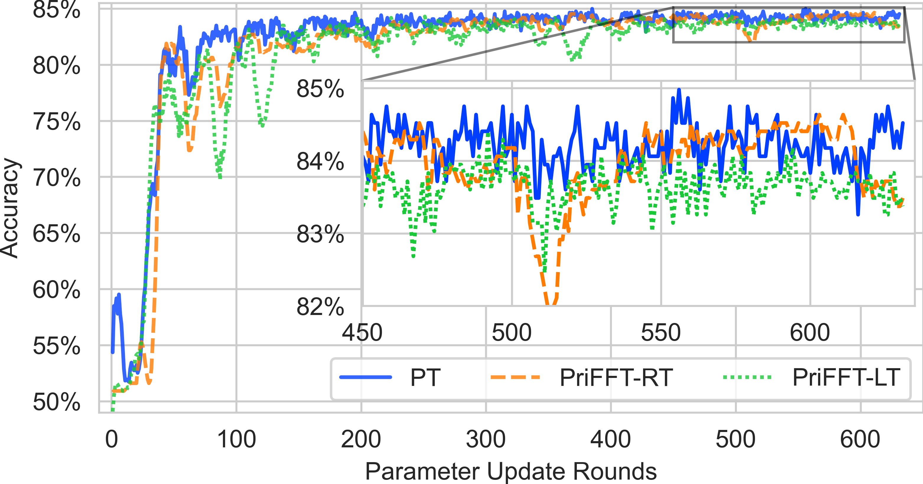
Figure 4: The relationship between the accuracy of BERT on SST-2 and parameter update rounds under different settings.

Fig. 4 illustrates how the accuracy on SST-2 of the fine-tuned model (BERT-base) varies with the aggregation times. There is little difference between ciphertext and plaintext fine-tuning before the model converges. The performance difference is that models fine-tuned with plaintext can achieve higher accuracy. The calculation error caused by the fine-tuning on encrypted samples does not bring significant model performance degradation for three reasons. Firstly, extensive training on the tunable parts of the model parameters can offset the impact of computational errors to a certain extent during the fine-tuning process. Secondly, the gradient value determines the change in model parameters, while the gradient during the parameter optimization step is the average of the gradients generated by a batch of training samples. In other words, each parameter update of the model is the average of multiple calculation results, which reduces the impact of a single calculation error. Finally, model training often introduces randomness into the calculations to prevent overfitting. The success of introducing randomness in model training shows that model training is not sensitive to small amounts of noise.

TABLE III: Communication consumption of privacy-preserving fine-tuning for BERT with a batch of samples.

Batch Size		8	16	32	64
BERT-base	PriFFT-IT	61.43MB	104.78MB	191.86MB	364.90MB
	PriFFT-LT	25.27MB	28.46MB	39.21MB	59.60MB
	ABY2	210.05MB	402.06MB	786.06MB	1.46GB
BERT-large	PriFFT-IT	105.90MB	179.70MB	327.29MB	622.48MB
	PriFFT-LT	39.02MB	44.94MB	59.77MB	87.44MB
	ABY2	368.01MB	701.06MB	1.34GB	2.66GB

TABLE IV: Execution time of privacy-preserving fine-tuning for BERT with a batch of samples.

Batch Size			8	16	32	64
CPU	BERT-base	PriFFT-IT	0.83s	1.34s	2.42s	4.64s
		PriFFT-LT	0.67s	0.72s	1.17s	1.75s
		ABY2	1.04s	1.85s	4.28s	7.60s
	BERT-large	PriFFT-IT	1.52s	2.81s	4.53s	9.07s
		PriFFT-LT	0.74s	1.13s	1.95s	3.78s
		ABY2	1.53s	3.39s	6.80s	11.52s
GPU	BERT-base	PriFFT-IT	0.78s	1.01s	1.41s	2.98s
		PriFFT-LT	0.51s	0.55s	0.58s	1.23s
		ABY2	1.12s	1.41s	3.15s	6.73s
	BERT-large	PriFFT-IT	1.05s	1.36s	1.88s	3.12s
		PriFFT-LT	0.64s	0.68s	0.73s	0.99s
		ABY2	1.48s	1.86s	5.29s	10.51s

We next discuss the communication and computational consumption during privacy-preserving fine-tuning. TABLE III summarizes the communication overhead when fine-tuning BERT with a batch of samples under different privacy-preserving implementations. TABLE IV summarizes the execution time of corresponding privacy-preserving fine-tuning.

We also discuss the communication consumption and execution time of privacy-preserving fine-tuning of BERT through all training samples of downstream tasks. Due to the space limitation, the results are given in APPENDIX D.

VII-C Protocol Analysis

In this section, we discuss the communication overhead and execution time of protocols proposed in Section V. Table V summarizes the overhead of the reciprocal calculation on shared inputs under different settings. As discussed in Section V-C, the sign consistency of the initial values and the input data directly affects the reciprocal accuracy. The inputs to the softmax and tanh functions are positive, so we consider the overhead of calculating the reciprocal when the signs of inputs are deterministic (DS) in the evaluation. For the more general case where the input signs are random (RS), we also give the corresponding overhead in the TABLE V. The ABY2-based implementation uses MSB to determine the input signs.

TABLE V: Communication overhead and execution time of secure reciprocal calculation under different settings.

Input Size

Communication Overhead

Execution Time

Random signs

Deterministic signs

Random signs

Deterministic signs

PriFFT-IT

PriFFT-LT

ABY2

PriFFT-IT

PriFFT-LT

ABY2

PriFFT-IT

PriFFT-LT

ABY2

PriFFT-IT

PriFFT-LT

ABY2

$10^{3}$

853.52KB

619.14KB

5.99MB

734.38KB

484.38KB

1.22MB

0.31s

0.29s

0.42s

0.24s

0.19s

0.39s

$10^{4}$

5.33MB

6.05MB

59.91MB

7.17MB

4.73MB

12.21MB

0.47s

0.31s

0.69s

0.41s

0.24s

0.51s

$10^{5}$

83.35MB

60.46MB

599.10MB

71.72MB

47.30MB

122.07MB

0.71s

0.64s

2.53s

0.68s

0.62s

1.38s

$10^{6}$

833.51MB

604.63MB

5.85GB

717.16MB

473.02MB

1.19GB

5.52s

4.16s

22.17s

3.51s

1.55s

5.51s

TABLE V shows that when the signs of shared input are deterministic, the overhead of the secure calculation is less than the case where the signs are random. It comes from that the comparison between shared inputs and 0 can be omitted when dealing with the inputs with deterministic signs. When the signs of shared inputs are random, the amount of consumed resources caused by the secure comparison in PriFFT-IT and PriFFT-LR is much less than that implementation with ABY2. PriFFT-IT and PriFFT-LT apply DPF to securely compare the shared inputs, while ABY2 applies MSB to compare the inputs with 0. DPF only brings a small amount of communication consumption in the online phase. The execution time of PriFFT-RS is slightly longer than that of PriFFT-DS. The communication consumption of secure comparison via MSB is much higher than that of DPF. Therefore, the execution time of ABY2-RS increases significantly, most of which is spent on communication.

TABLE VI: Overhead of secure $e^{x}$.

Input Size		$10^{3}$	$10^{4}$	$10^{5}$	$10^{6}$	$10^{7}$
Comm	PriFFT-IT	195KB	1.9MB	19MB	190MB	1.8GB
	PriFFT-LT	132KB	1.3MB	12.9MB	129MB	1.27GB
	ABY2	320KB	3.1MB	31MB	312MB	3.0GB
Time	PriFFT-IT	0.52s	0.63s	1.21s	1.62s	9.55s
	PriFFT-LT	0.41s	0.57s	0.73s	1.01s	8.21s
	ABY2	0.55s	0.78s	1.49s	2.03s	11.56s

TABLE VII: Overhead of secure $\mathrm{Tanh}(x)$.

Input Size		$10^{3}$	$10^{4}$	$10^{5}$	$10^{6}$	$10^{7}$
Comm	PriFFT-IT	968KB	9.46MB	95MB	946MB	9.2GB
	PriFFT-LT	656KB	6.41MB	64MB	640MB	6.3GB
	ABY2	1.6MB	15.9MB	159MB	1.5GB	15.4GB
Time	PriFFT-IT	0.82s	1.21s	1.88s	4.27s	42.81s
	PriFFT-LT	0.77s	0.84s	1.15s	2.94s	35.36s
	ABY2	0.91s	1.35s	2.60s	7.68s	54.16s

Similarly, we evaluate the overhead of secure $e^{x}$ and $\mathrm{Tanh}(x)$ under different settings. As discussed in Section V-B, we approximate $e^{x}$ through multiple multiplications. The proposed secure $e^{x}$ protocol reduces the amount of data exchanged during multiplication and lowers communication consumption. Therefore, both the implementation with PriFFT-IT and PriFFT-LT realize lower communication overhead compared to the implementation with ABY2. The secure $\mathrm{Tanh}(x)$ invokes a secure $e^{x}$, a secure reciprocal calculation with deterministic input signs, and a secure multiplication as discussed in Section B-C. As a result, the overhead of the secure $\mathrm{Tanh}(x)$ is close to the sum of the overheads of the secure $e^{x}$ and the secure reciprocal calculation with deterministic input signs.

TABLE VIII: Communication overhead and execution time of secure dropout under different settings.

Input Size

Communication Overhead

Execution Time

Static Dropout

Dynamic Dropout

Static Dropout

Dynamic Dropout

PriFFT-IT

PriFFT-LT

ABY2

PriFFT-IT

PriFFT-LT

ABY2

PriFFT-IT

PriFFT-LT

ABY2

PriFFT-IT

PriFFT-LT

ABY2

$10^{3}$

23.44KB

15.63KB

39.06KB

64.45KB

56.64KB

4.77MB

0.23s

0.12s

0.31s

0.31s

0.23s

0.39s

$10^{4}$

234.38KB

156.25KB

390.63KB

644.53KB

566.41KB

47.70MB

0.37s

0.23s

0.44s

0.48s

0.46s

0.71s

$10^{5}$

2.29MB

1.53MB

3.81MB

6.29MB

5.31MB

477.03MB

0.62s

0.56s

0.76s

0.54s

0.59s

2.56

$10^{6}$

22.89MB

15.26MB

38.15MB

62.94MB

55.31MB

4.66GB

0.98s

0.84s

1.05s

2.75s

2.53s

18.05s

The overhead of the secure dropout is summarized in TABLE VIII. In the static dropout, the key generation in the offline phase generates random numbers and stores the dropout factor in the key, where the dropout factors depend on the generated numbers and the given dropout probability. Therefore, each party only performs a secure multiplication of shared input and dropout factors in the online phase to obtain the dropout result. The key retains the random numbers in the dynamic dropout without directly calculating the dropout factors. In the online phase, each party performs a secure comparison between the dynamic dropout probability and random numbers to calculate the dropout factors. The consumption of the dynamic dropout is greater than the consumption of the static dropout due to the secure computation. However, compared with MSB, PriFFT significantly reduces communication consumption in the online phase, which only incurs a slight consumption increase for the implementation with IT and RT.

VII-D Error Evaluation

PriFFT approximates $e^{x}$, $1/x$, and $\mathrm{Tanh}(x)$ by the secure computation. Meanwhile, we provide different truncation methods in the paper. In this section, we combine evaluation to discuss the errors of each secure calculation under different settings. Evaluation first calculates the relative error between the approximated results from the secure computation and the exact results computed in plaintext with PyTorch. We use the error rate to analyze the error in the secure computation, i.e., the percentage between the relative errors and the exact values. The inputs are $10^{5}$ random values from 0 to 1, and the provided results are the mean of $10^{5}$ error rates for each case.

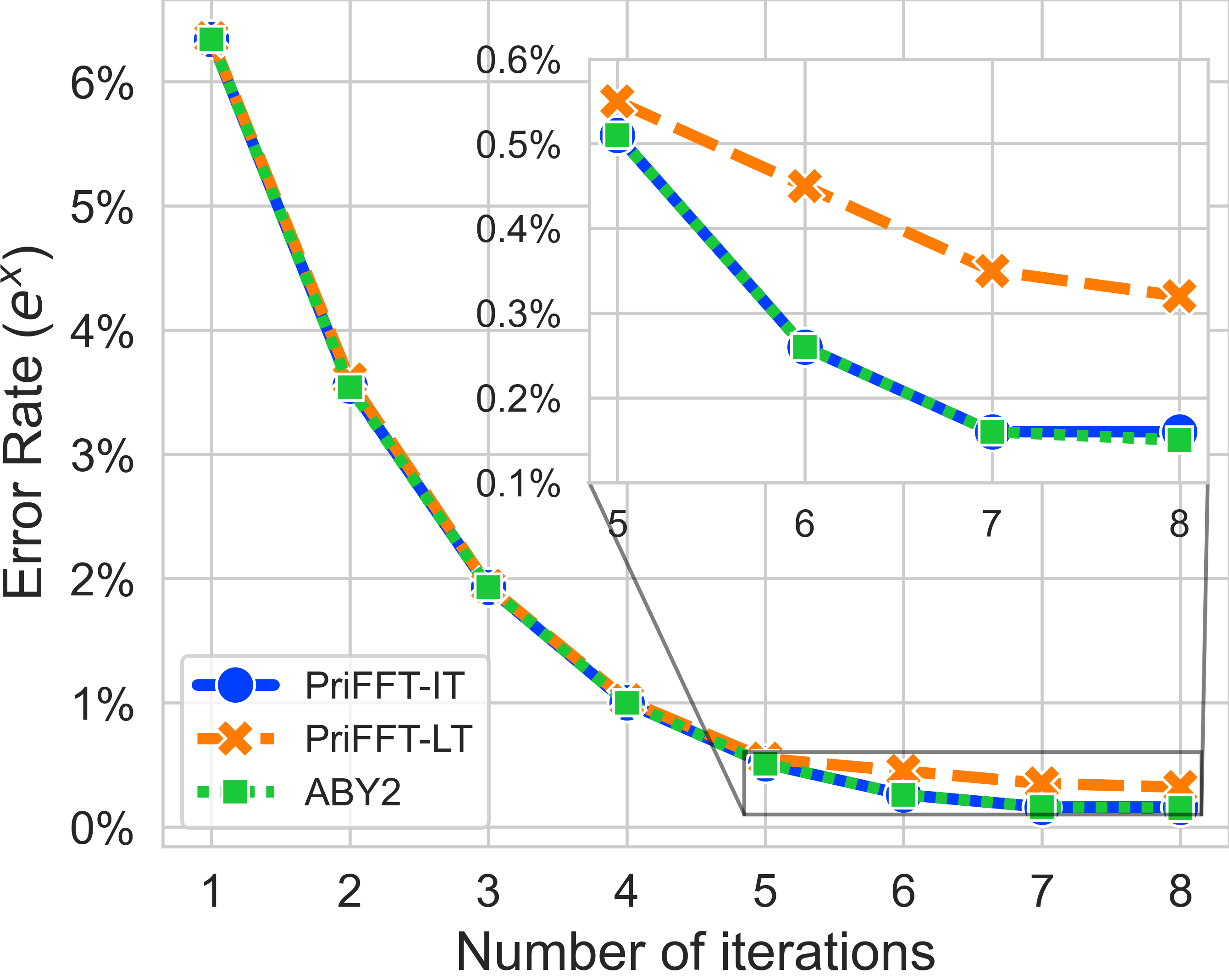
(a) $e^{x}$

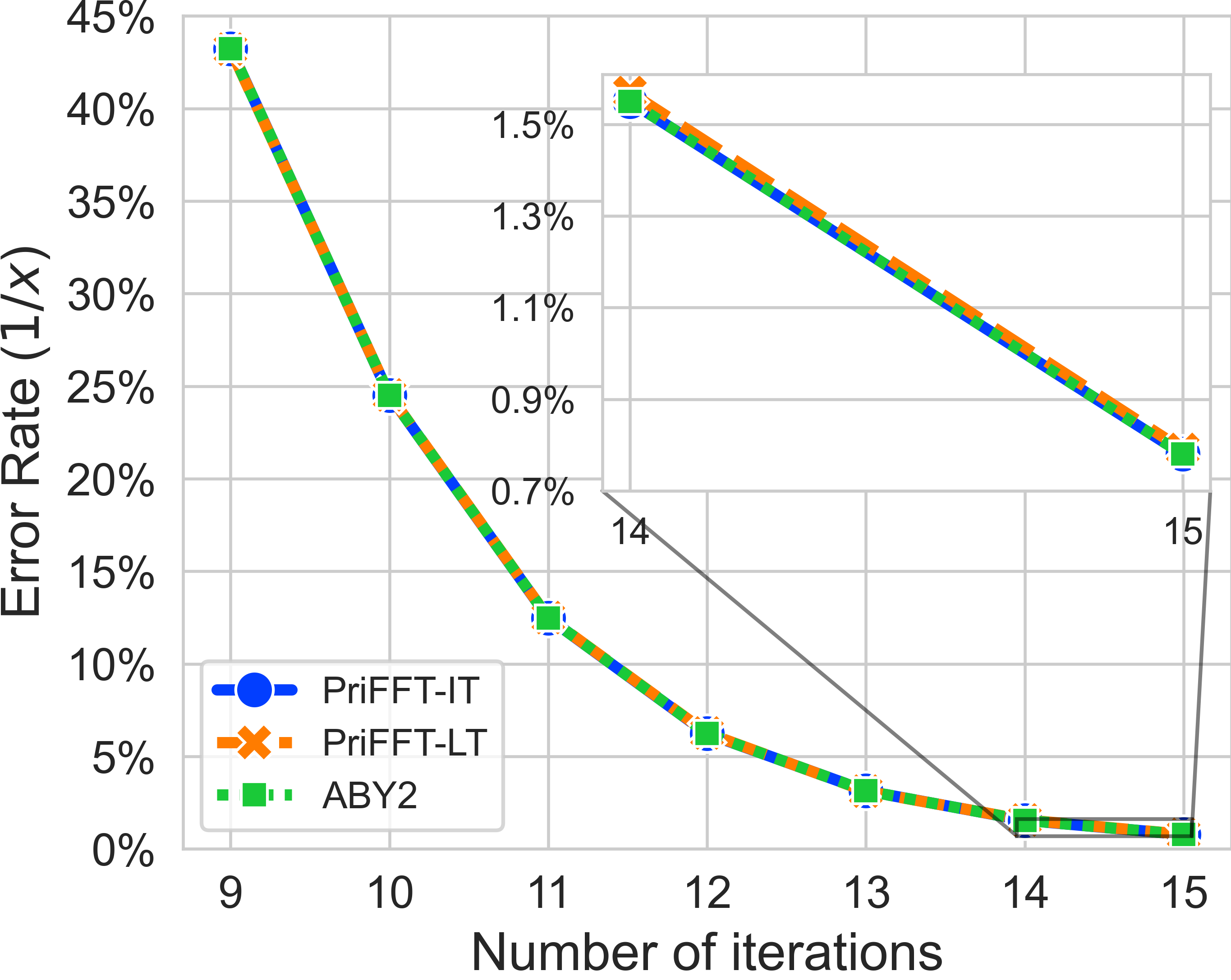
(b) $1/x$

Figure 5: The impact of the number of iterations on the error rates of the secure $e^{x}$ and reciprocal calculation.

Fig. 5 presents the impact of the number of iterations $m_{\exp}$ and $m_{\mathrm{recip}}$ on the error rates of secure $e^{x}$ and $\mathrm{Tanh}(x)$. For secure $e^{x}$, when $m_{\exp}<5$, truncation methods have no significant impact on the error rate, as shown in Fig. 5(a). When the number of iterations is insufficient, the error is relatively large. In this case, the difference between iterative and local truncations is too small to impact the error rate significantly. The error rate of secure $e^{x}$ decreases as $m_{\exp}$ increases. Meanwhile, differences in truncation methods begin to have an impact on error. Experimental results show that it is difficult to effectively reduce the error rates by further increasing the number of iterations. It comes from that the experiment takes 16 bits to represent the fractional part of fixed-point numbers. More accurate results rely on more bits to represent the fractional part.

Fig. 5(b) presents the error rate of the secure reciprocal calculation under different $m_{\mathrm{recip}}$. Despite applying a higher number of iterations, the secure reciprocal calculation does not have a lower error rate than the secure $e^{x}$. The reason is that different approximation calculations were performed during the iteration process. As shown in Equation 4, setting the number of iterations to 8 for the secure $e^{x}$ implies that $n=2^{8}=256$ for $(1+x/n)^{n}$. However, the number of iterations equals the number of approximations for the secure reciprocal calculation, leading the secure $e^{x}$ to realize lower error rates with fewer iterations.

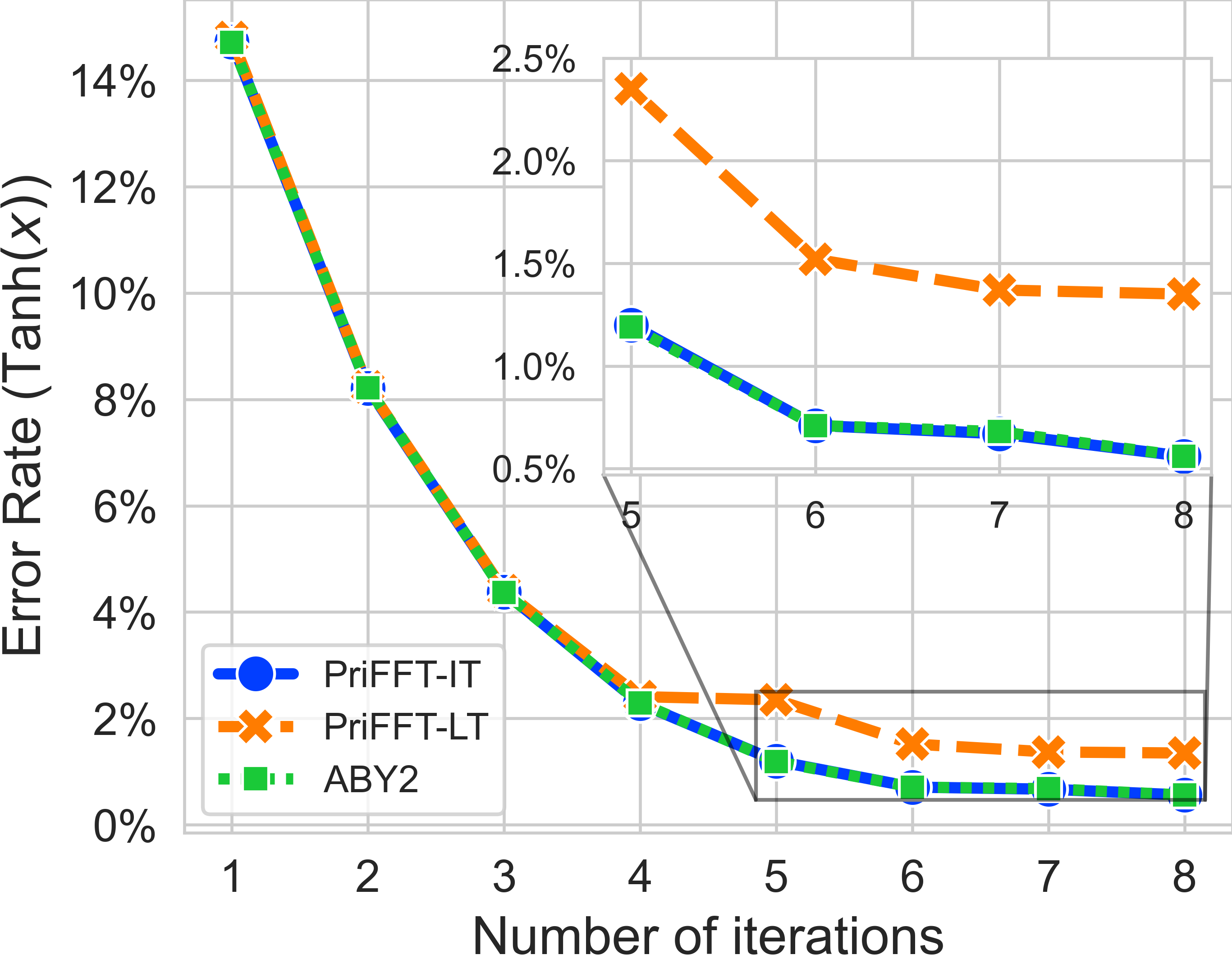
(a) $e^{x}$

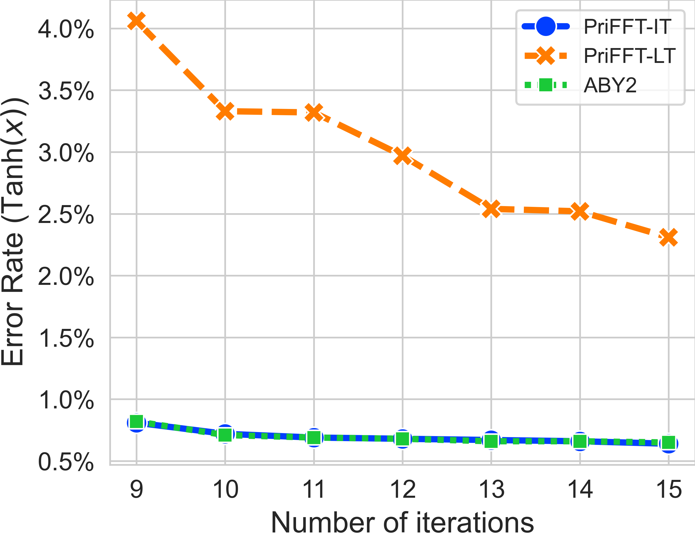
(b) $1/x$

Figure 6: The impact of $m_{\exp}$ and $m_{\mathrm{recip}}$ on the error rates of the secure $\mathrm{Tanh}(x)$.

Fig. 6 provides the impact of $m_{\exp}$ and $m_{\mathrm{recip}}$ on the error rates of $\mathrm{Tanh}(x)$. The implementation of the secure $\mathrm{Tanh}(x)$ involves the secure $e^{x}$ and the secure reciprocal calculation. Fig. 6(a) presents the error rate of the secure $\mathrm{Tanh}(x)$ under different $m_{\exp}$ when $m_{\mathrm{recip}}=15$. Fig. 6(a) presents the error rate of the secure $\mathrm{Tanh}(x)$ under different $m_{\mathrm{recip}}$ when $m_{\exp}=8$. Although the error rate of the secure reciprocal calculation is higher than that of the secure $e^{x}$, the secure reciprocal calculation has a minor effect on the error rate of the secure $\mathrm{Tanh}(x)$ compared to the secure $e^{x}$. As shown in the definition of $\mathrm{Tanh}(x)$, the input of the secure reciprocal calculation is $e^{2x}+1>1$. The secure reciprocal calculation results in the secure $\mathrm{Tanh}(x)$ varying from 0 to 1. As a result, the secure reciprocal calculation has a minor effect on the error rate of the secure $\mathrm{Tanh}(x)$ compared to the secure $e^{x}$.

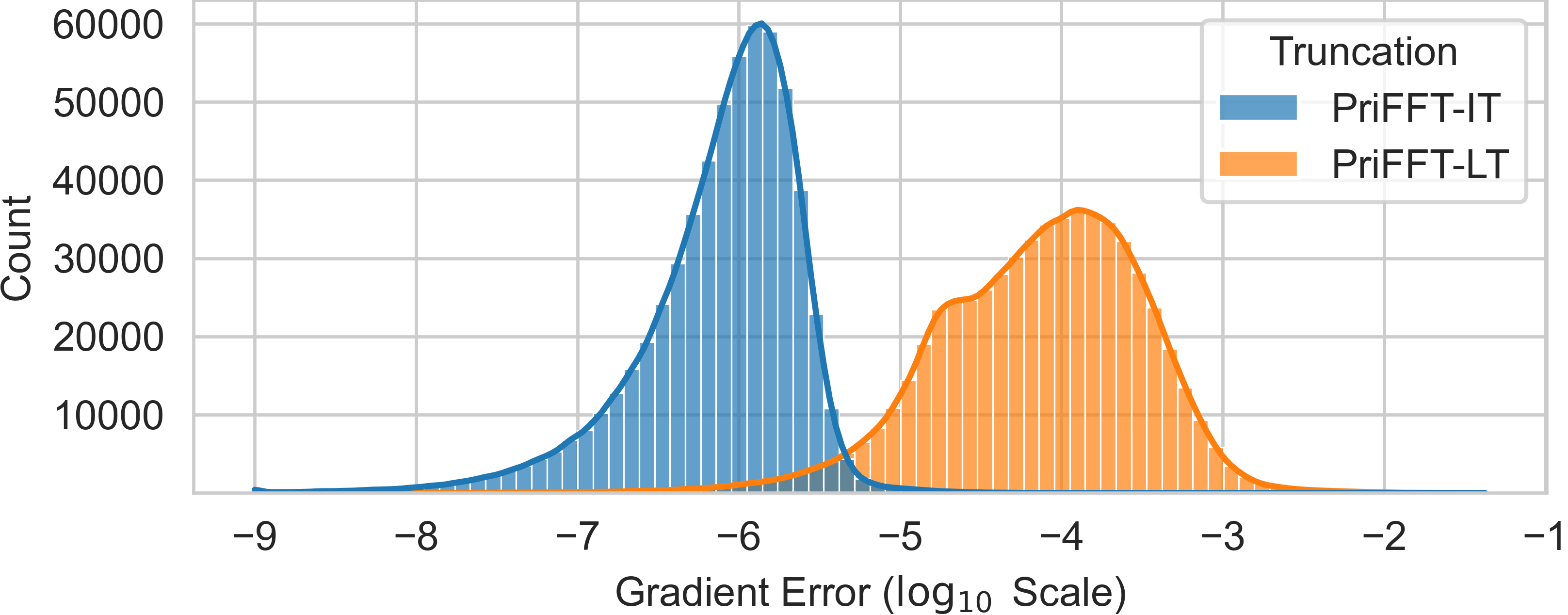
Figure 7: The distribution of gradient error with different settings.

We further analyze the impact of different truncation methods on the model gradient error. Fig. 7 compares the error of weight gradients in the pooler layer generated by 32 samples with different truncation methods. PriFFT-IT achieves smaller errors, owing to its higher accuracy in secure computation. However, most of the errors in PriFFT-LT lie between $10^{-3}$ and $10^{-6}$, which is still minor compared to the gradients. Therefore, it is more practical to employ LT to reduce communication consumption during the early stages of fine-tuning and subsequently apply IT to enhance calculation accuracy in the later stages of fine-tuning.

VIII Conclusion

In this paper, we first discuss the privacy concern in federated fine-tuning, i.e., both LLMs parameters and uploaded gradients would cause privacy leakage. To solve the above privacy problem, we present PriFFT to implement federated fine-tuning of LLMs, while protecting both LLMs parameters and uploaded gradients. In PriFFT, clients and the server additively share LLM parameters and the inference results, while the privacy-preserving fine-tuning is implemented based on the shared values. Each party cannot directly access the plaintext LLM parameters and clients’ gradients in the privacy-preserving fine-tuning. Due to the large amount of LLM parameters, fine-tuning LLMs on shared values requires substantial computation and communication resources. Therefore, we propose several FSS-based secure protocols, including secure power function, $e^{x}$, reciprocal calculation, softmax function, $\mathrm{Tanh}(x)$, dropout function, and tensor product, to implement the privacy-preserving federated fine-tuning and reduce resource requirement. We evaluate PriFFT with ABY2-based privacy-preserving federated fine-tuning. Evaluation results show that PriFFT realizes the same fine-tuned model accuracy while significantly reducing the communication overhead and the execution time.

Appendix A Preliminary Supplement

A-A Arithmetic Secret Sharing

A-A1 Sharing Semantics

The server and each client in the proposed mechanism works on two-party computation model where parties $\{P_{0},P_{1}\}$ are connected by a bidirectional synchronous channel. Specifically, we consider the following sharing semantics:

• Shared Values. For two $l$-bit shares $\left\langle x\right\rangle_{0}$ and $\left\langle x\right\rangle_{1}$ of $x$, we have $\left\langle x\right\rangle_{0}+\left\langle x\right\rangle_{1}\equiv x\;(\mathrm{mod}\;2^{l})$ with $\left\langle x\right\rangle_{0},\left\langle x\right\rangle_{1}\in\mathbb{Z}_{2^{l}}$.

• Sharing. The secret owner $P_{b}$ sample random value $r\in\mathbb{Z}_{2^{l}}$, sets $\left\langle x\right\rangle_{b}=x-r$, and sends $\left\langle x\right\rangle_{1-b}=r$ to $P_{1-b}$.

• Restore. When $P_{b}$ needs to restore $x$, $P_{1-b}$ sends $\left\langle x\right\rangle_{1-b}$ to $P_{b}$ who restores $x=\left\langle x\right\rangle_{0}+\left\langle x\right\rangle_{1}$.

A-A2 Operations

The addition and multiplication of shares are evaluated as follows:

• Addition. Given shares $\left\langle x\right\rangle_{b}$ and $\left\langle y\right\rangle_{b}$, $P_{b}$ locally computes $\left\langle x+y\right\rangle_{b}=\left\langle x\right\rangle_{b}+\left\langle y\right\rangle_{b}$.

• Multiplication. The multiplication of shares depends on Beaver triples $\{A,B,C\}\subseteq\mathbb{Z}_{2^{l}}$ generated in the offline phase such that $\left\langle C\right\rangle_{b}=\left\langle A\cdot B\right\rangle_{b}$. When $P_{b}$ computes $\left\langle x\cdot y\right\rangle_{b}$, $P_{b}$ sets $\left\langle E\right\rangle_{b}=\left\langle x\right\rangle_{b}-\left\langle A\right\rangle_{b}$ and $\left\langle F\right\rangle_{b}=\left\langle y\right\rangle_{b}-\left\langle B\right\rangle_{b}$. Both parties restore $E$ and $F$ by exchanging corresponding shares. Parties $P_{b}$ computes $\left\langle x\cdot y\right\rangle_{b}=b\cdot E\cdot F+F\cdot\left\langle A\right\rangle_{b}+E\cdot\left\langle B\right\rangle_{b}+\left\langle C\right\rangle_{b}$.

A-B Function Secret Sharing

Definition 2 (FSS: syntax [14]).

A 2-party FSS scheme is a pari of algorithms $(\mathrm{Gen,Eval})$ such that:

• $\mathrm{Gen}(1^{\lambda},\hat{f})$ is a probabilistic polynomial-time (PPT) key generation algorithm that outputs a pair of keys $\left(k_{0},k_{1}\right)$ where $\lambda$ is a security parameter and $\hat{f}\in\left\{0,1\right\}^{*}$ is a description of a function $f$. The function description $\hat{f}$ is assumed to contain descriptions of input and output groups $\mathbb{G}^{\mathrm{in}}$, $\mathbb{G}^{\mathrm{out}}$.

• $\mathrm{Eval}(\sigma,k_{\sigma},x)$ is a polynomial-time evaluation algorithm that outputs a group element $y_{\sigma}\in\mathbb{G}^{\mathrm{out}}$ (the value of $f_{\sigma}(x)$) where $\sigma\in\left\{0,1\right\}$ (party index), $k_{\sigma}$ (key defining $f_{\sigma}:\mathbb{G}^{\mathrm{in}}\rightarrow\mathbb{G}^{\mathrm{out}}$) and $x\in\mathbb{G}^{\mathrm{in}}$ (input for $f_{\sigma}$).

Definition 3 (Offset function family and FSS gates [32]).

Assume that $\mathcal{G}=\left\{g:\mathbb{G}^{\mathrm{in}}\rightarrow\mathbb{G}^{\mathrm{out}}\right\}$ is a computation gate parameterized by input and output groups $\mathbb{G}^{\mathrm{in}}$ and $\mathbb{G}^{\mathrm{out}}$, the offset function family $\hat{\mathcal{G}}$ of $\mathcal{G}$ is given by

$$\hat{\mathcal{G}}:=\left\{\begin{array}[]{l|l}g^{\left[r^{\text{in}},r^{\text{out}}\right]}:\mathbb{G}^{\text{in}}\rightarrow\mathbb{G}^{\text{out}}&\begin{aligned} &g:\mathbb{G}^{\text{in}}\rightarrow\mathbb{G}^{\text{out}}\in\mathcal{G},\\ &r^{\text{in}}\in\mathbb{G}^{\text{in}},\\ &r^{\text{out}}\in\mathbb{G}^{\text{out}}\end{aligned}\end{array}\right\},$$ (13)

where $g^{\left[r^{\mathrm{in}},r^{\mathrm{out}}\right]}(x):=g(x-r^{\mathrm{in}})+r^{\mathrm{out}}$ and $g^{\left[r^{\mathrm{in}},r^{\mathrm{out}}\right]}$ contains and explicit description of $r^{\mathrm{in}},r^{\mathrm{out}}$.

We consider a two-party computation (2PC) between each client and the server with a trusted dealer, secure against a probabilistic polynomial-time semi-honest adversary that passively corrupts one of the parties without deviating from the protocol. In the offline phase, the trusted dealer distributes input-independent correlated randomness to both parties. Using this pre-shared randomness, the parties execute the 2PC protocol in the online phase to securely compute the desired function.

Appendix B Other Protocols

B-A Multiplication with FSS

We denote the multiplication function gate with FSS by $\hat{\mathcal{G}}_{\mathrm{mul}}$ and the offset functions by:

$$\hat{g}_{\mathrm{mul},l,l}^{\left[r^{\mathrm{in}_{1}},r^{\mathrm{in}_{2}},r^{\mathrm{out}}\right]}(\hat{x},\hat{y})$$

$$= g_{\mathrm{mul},l,l}(\hat{x}-r^{\mathrm{in}_{1}},\hat{y}-r^{\mathrm{in}_{2}})+r^{\mathrm{out}}\mod 2^{l}$$

$$= (\hat{x}-r^{\mathrm{in}_{1}})\cdot(\hat{y}-r^{\mathrm{in}_{2}})+r^{\mathrm{out}}\mod 2^{l}$$

$$= \hat{x}\hat{y}-\hat{x}r^{\mathrm{in}_{2}}-\hat{y}r^{\mathrm{in}_{1}}+r^{\mathrm{in}_{1}}r^{\mathrm{in}_{2}}+r^{\mathrm{out}}\mod 2^{l}.$$ (14)

1 Requires: Input offsets $\{r^{\text{in}_{1}},r^{\text{in}_{2}}\}$, output offset $r^{\text{out}}$.

2 Output: Evaluation keys $(k_{0},k_{1})$.

3 Sample random $r^{\text{in}_{1}}_{0}$, $r^{\text{in}_{1}}_{1}$, $r^{\text{in}_{2}}_{0}$, $r^{\text{in}_{2}}_{1}$, $r^{\text{out}}_{0}$, $r^{\text{out}}_{1}\in\mathbb{Z}_{2^{l}}$, s.t., $r^{\text{in}_{1}}_{0}+r^{\text{in}_{1}}_{1}=r^{\text{in}_{1}}\mod 2^{l}$, $r^{\text{in}_{2}}_{0}+r^{\text{in}_{2}}_{1}=r^{\text{in}_{2}}\mod 2^{l}$, $r^{\text{out}}_{0}+r^{\text{out}}_{1}=r^{\text{out}}\mod 2^{l}$;

4 Sample random $q_{0},q_{1},\in\mathbb{Z}_{2^{l}}$, s.t., $q_{0}+q_{1}=r^{\text{in}_{1}}r^{\text{in}_{2}}\mod 2^{l}$;

5 For $b\in\{0,1\}$, let $k_{b}=r^{\text{in}_{1}}_{b}\|r^{\text{in}_{2}}_{b}\|q_{b}\|r^{\text{out}}_{b}$ ;

return $(k_{0},k_{1})$

Algorithm 9 Multiplications ($x\cdot y$) with FSS in the offline stage $\mathrm{Gen}^{\mathrm{mul}}_{l,l}(r^{\text{in}_{1}},r^{\mathrm{in}_{2}},r^{\text{out}})$ .

1 Requires: Evaluation keys $(k_{0},k_{1})$, additive shares $(\left\langle\hat{x}\right\rangle_{0},\left\langle\hat{x}\right\rangle_{1})$ of $\hat{x}$ with offset $r^{\text{in}_{1}}$, additive shares $(\left\langle\hat{y}\right\rangle_{0},\left\langle\hat{y}\right\rangle_{1})$ of $\hat{y}$ with offset $r^{\text{in}_{2}}$, scale factor $s$.

2 Output: Shares of $(\hat{x}-r^{\text{in}_{1}})(\hat{y}-r^{\text{in}_{2}})+r^{\text{out}}$.

3 Restore $\hat{x}=x+r^{\mathrm{in}_{1}}$ from shares of $\hat{x}$ ;

4 Restore $\hat{y}=y+r^{\mathrm{in}_{2}}$ from shares of $\hat{y}$ ;

5 for $b\in\{0,1\}$ do

6    Parse $k_{b}=r^{\text{in}_{1}}_{b}\|r^{\text{in}_{2}}_{b}\|q_{b}\|r^{\text{out}}_{b}$;

7    $\left\langle\hat{t}\right\rangle_{b}=\mathrm{Trunc}(b\hat{x}\hat{y}-\hat{x}r^{\mathrm{in}_{2}}_{b}-\hat{y}r^{\mathrm{in}_{1}}_{b}+q_{b},s)+r^{\text{out}}_{b}\mod 2^{l};$

return $(\left\langle\hat{t}\right\rangle_{0},\left\langle\hat{t}\right\rangle_{1})$

Algorithm 10 Multiplications ($x\cdot y$) with FSS in the online stage $\mathrm{Eval}^{\mathrm{mul}}_{l,l}(b,k_{b},\left\langle\hat{x}\right\rangle_{b},\left\langle\hat{y}\right\rangle_{b})$

Algorithm 9 presents the offline stage of the secure multiplications with FSS. Algorithm 10 presents the online stage of the secure multiplications function with FSS.

B-B Square Function and Power Function

We define the square function gate $\mathcal{G}_{\mathrm{square}}$ as the family of functions $g_{\mathrm{square},l}:\mathbb{Z}_{2^{l}}\rightarrow\mathbb{Z}_{2^{l}}$ with input group $\mathbb{G}^{\mathrm{in}}=\mathbb{Z}_{2^{l}}$, output group $\mathbb{G}^{\mathrm{out}}=\mathbb{Z}_{2^{l}}$, and $g_{\mathrm{square},l}(x):=x^{2}$.

We denote the square function gate with FSS by $\hat{\mathcal{G}}_{\mathrm{squar}}$ and the offset functions by:

$$\hat{g}_{\mathrm{square},l}^{\left[r^{\mathrm{in}},r^{\mathrm{out}}\right]}(\hat{x}) =g_{\mathrm{square},l}(\hat{x}-r^{\mathrm{in}})+r^{\mathrm{out}}\mod 2^{l}$$

$$=(\hat{x}-r^{\mathrm{in}})\cdot(\hat{x}-r^{\mathrm{in}})+r^{\mathrm{out}}\mod 2^{l}$$

$$=\hat{x}^{2}-2\hat{x}r^{\mathrm{in}}+(r^{\mathrm{in}})^{2}+r^{\mathrm{out}}\mod 2^{l}.$$ (15)

1 Requires: Input offset $r^{\text{in}}$, output offset $r^{\text{out}}$.

2 Output: Evaluation keys $(k_{0},k_{1})$.

3 Sample random $r^{\text{in}}_{0}$, $r^{\text{in}}_{1}$, $r^{\text{out}}_{0}$, $r^{\text{out}}_{1}\in\mathbb{Z}_{2^{l}}$, s.t., $r^{\text{in}}_{0}+r^{\text{in}}_{1}=r^{\text{in}}\mod 2^{l}$, $r^{\text{out}}_{0}+r^{\text{out}}_{1}=r^{\text{out}}\mod 2^{l}$;

4 Sample random $q_{0}$, $q_{1}\in\mathbb{Z}_{2^{l}}$, s.t., $q_{0}+q_{1}=(r^{\text{in}})^{2}\mod 2^{l}$;

5 For $b\in\{0,1\}$, let $k_{b}=r^{\text{in}}_{b}\|q_{b}\|r^{\text{out}}_{b}$ ;

return $(k_{0},k_{1})$

Algorithm 11 Square function ($x^{2}$) with FSS in the offline stage $\mathrm{Gen}^{\mathrm{square}}_{l}(r^{\text{in}},r^{\text{out}})$ .

Algorithm 11 presents the offline stage of the secure square function with FSS. In the offline stage, the input and output offset are split into two additive shares $\left\{r^{\mathrm{in}}_{0},r^{\mathrm{in}}_{1}\right\}$ and $\left\{r^{\mathrm{out}}_{0},r^{\mathrm{out}}_{1}\right\}$ (line 3). Besides, the multiplication result of $(r^{\mathrm{in}})^{2}$ is also spilt into two additive shares $\left\{q_{0},q_{1}\right\}$ (line 4). Since the computation is performed on a $\mathbb{Z}_{2^{l}}$ ring, the bitwidth of $(r^{\mathrm{in}})^{2}$, $q_{0}$, and $q_{1}$ are $l$. Therefore, the key size of the secure square function with FSS is $3l$ bits for each party, which is the same as the implementation based on ASS where keys include Beaver triples $\left\{A,B,C\right\}$.

1 Requires: Evaluation keys $(k_{0},k_{1})$, additive shares $(\left\langle\hat{x}\right\rangle_{0},\left\langle\hat{x}\right\rangle_{1})$ of $\hat{x}$ with offset $r^{\text{in}}$, scale factor $s$.

2 Output: Shares of $(\hat{x}-r^{\text{in}})^{2}+r^{\text{out}}$.

3 Restore $\hat{x}=x+r^{\mathrm{in}}$ from shares of $\hat{x}$ ;

4 for $b\in\{0,1\}$ do

5    Parse $k_{b}=r^{\text{in}}_{b}\|q_{b}\|r^{\text{out}}_{b}$;

6    $\left\langle\hat{t}\right\rangle_{b}=\mathrm{Trunc}(b\hat{x}^{2}-2r^{\mathrm{in}}_{b}\hat{x}+q_{b},s)+r^{\text{out}}_{b}\mod 2^{l};$

return $(\left\langle\hat{t}\right\rangle_{0},\left\langle\hat{t}\right\rangle_{1})$

Algorithm 12 Square function ($x^{2}$) with FSS in the online stage $\mathrm{Eval}^{\mathrm{square}}_{l}(b,k_{b},\left\langle\hat{x}\right\rangle_{b})$

Algorithm 12 presents the online stage of the secure square function with FSS. Each party exchanges their shares of $\hat{x}$ to restore $\hat{x}=x+r^{\mathrm{in}}$ (line 3). The shares of results are computed according to Equation (B-B) (line 6) Since each party cannot obtain $r^{\mathrm{in}}$, restoring $\hat{x}$ with the input offset does not leak information about $x$. The input $\hat{x}$ of Algorithm 12 is masked by the input offset $r^{\mathrm{in}}$. Meanwhile, $\hat{x}$ is the output of a previous FSS gate with an output offset $r^{\mathrm{out}^{\prime}}$. The correctness of the square function gate with FSS lies in setting $r^{\mathrm{in}}$ equal to the output offset of the previous FSS gate, $r^{\mathrm{out}^{\prime}}$, in the offline stage.

Generally, $\mathrm{Gen}^{\mathrm{square}}_{l}$ is the key generation in the offline stage and outputs keys $(k_{0},k_{1})$ belonging to the server and the client. In the online stage, $\mathrm{Eval}^{\mathrm{square}}_{l}$ uses $(k_{0},k_{1})$ and the shared inputs of $x$ to calculate the shares of $x^{2}$.

The power function is implemented based on exponentiation by squaring, i.e.,

$$f(x,n)=\begin{cases}1&\text{if }n=0;\\ x&\text{if }n=1;\\ (f(x,n/2))^{2}&\text{if }n\text{ is even};\\ x\times(f(x,(n-1)/2))^{2}&\text{if }n\text{ is odd}.\end{cases}$$ (16)

For convenience, we consider the case where $n=2^{m}$ to describe the secure power function. In the case of $n\neq 2^{m}$, the commutation can be implemented by combining Equation (16) and the following proposed algorithms.

1 Requires: Input offset $r^{\text{in}}$, output offset $r^{\text{out}}$, intermediate offsets $\mathbf{r}=\{r^{(1)},\cdots,r^{(m)}\}$, power $2^{m}$.

2 Output: Evaluation keys $(k_{0},k_{1})$.

3 Sample random $r^{\text{in}}_{0}$, $r^{\text{in}}_{1}$, $r^{\text{out}}_{0}$, $r^{\text{out}}_{1}\in\mathbb{Z}_{2^{l}}$, s.t., $r^{\text{in}}_{0}+r^{\text{in}}_{1}=r^{\text{in}}\mod 2^{l}$, $r^{\text{out}}_{0}+r^{\text{out}}_{1}=r^{\text{out}}\mod 2^{l}$;

4 foreach $r_{i}\in\{r^{(1)},\cdots r^{({m})}\}$ do

5    Sample random $r^{(i)}_{0}$, $r^{(i)}_{1}$, $q^{(i)}_{0}$, $q^{(i)}_{1}\in\mathbb{Z}_{2^{l}}$, s.t., $r^{(i)}_{0}+r^{(i)}_{1}=r^{(i)}\mod 2^{l}$, $q^{(i)}_{0}+q^{(i)}_{1}=\left[r^{(i)}\right]^{2}\mod 2^{l}$;

6   

7For $b\in\{0,1\}$, let $k_{b}=r^{\text{in}}_{b}\|r^{(1)}_{b}\|q^{(1)}_{b}\|\cdots\|r^{(m)}_{b}\|q^{(m)}_{b}\|r^{\text{out}}_{b}$;

return $(k_{0},k_{1})$

Algorithm 13 Power function ($x^{2^{m}}$) with FSS in the offline stage $\mathrm{Gen}^{\mathrm{power}}_{l}(r^{\text{in}},r^{\text{out}},\mathbf{r},2^{m})$.

1 Requires: Evaluation keys $(k_{0},k_{1})$, additive shares $(\left\langle\hat{x}\right\rangle_{0},\left\langle\hat{x}\right\rangle_{1})$ of $\hat{x}$ with offset $r^{\text{in}}$, scale factor $s$.

2 Output: Shares of $(\hat{x}-r^{\text{in}})^{2}+r^{\text{out}}$.

3 ;

4 for $b\in\{0,1\}$ do

5    Parse $k_{b}=r^{\text{in}}_{b}\|r^{(1)}_{b}\|q^{(1)}_{b}\|\cdots\|r^{(m)}_{b}\|q^{(m)}_{b}\|r^{\text{out}}_{b}$;

6    $\left\langle\hat{t}_{0}\right\rangle_{b}=\left\langle\hat{x}\right\rangle_{b}+r_{n}^{\mathrm{in}};$ for $i=1\>\mathrm{to}\>m$ do

7       if $i<m_{\exp}$ then

8          $k_{b}^{\mathrm{square}}=r^{(i)}_{b}\|q^{(i)}_{b}\|r^{(i+1)}_{b}$ ;

9         

10      else

11          $k_{b}^{\mathrm{square}}=r^{(i)}_{b}\|q^{(i)}_{b}\|r^{\text{out}}_{b}$ ;

12      $\left\langle\hat{t}_{i}\right\rangle_{b}=\mathrm{Eval}^{\mathrm{square}}_{l}(b,k_{b}^{\mathrm{square}},\left\langle\hat{t}_{i-1}\right\rangle_{b})$

13      

14   

return $(\left\langle\hat{t_{m}}\right\rangle_{0},\left\langle\hat{t_{m}}\right\rangle_{1})$

Algorithm 14 Power function ($x^{2^{m}}$) with FSS in the online stage $\mathrm{Eval}^{\mathrm{power}}_{l}(b,k_{b},\left\langle\hat{x}\right\rangle_{b},2^{m})$

B-C Softmax and Hyperbolic Tangent

We implement the softmax gate by combining the natural exponential function gate with the reciprocal gate as shown in Algorithm 15. The softmax function involves the normalization of $K$ inputs, we use $\mathbf{x}\in\mathbb{Z}^{K}_{2^{l}}$ and $\mathbf{r}\in\mathbb{Z}^{K}_{2^{l}}$ to represent the inputs and offsets, respectively. The output offsets in the key generation of natural exponential functions are $\emptyset$, which means the outputs are not masked by the offset and are additive shared.

1 Requires: Input offsets $\mathbf{r}^{\text{in}}$, output offset $\mathbf{r}^{\text{out}}$, intermediate offsets $(\mathbf{r}^{\mathrm{exp}},\mathbf{r}^{\mathrm{recip}})$ for $\mathrm{Gen}^{\mathrm{exp}}_{l}$ and $\mathrm{Gen}^{\mathrm{recip}}_{l}$, input offset $\mathbf{r}^{\mathrm{in}^{\prime}}$ for $\mathrm{Gen}^{\mathrm{recip}}_{l}$, input offset $\mathbf{r}^{\mathrm{in}^{\prime\prime}}$ for multiplication.

2 Output: Evaluation keys $(k_{0},k_{1})$.

3 $(k_{0}^{\mathrm{exp}},k_{1}^{\mathrm{exp}})=\mathrm{Gen}^{\mathrm{exp}}_{K\times l}(\mathbf{r}^{\text{in}},\emptyset,\mathbf{r}^{\mathrm{exp}})$;

4 $(k_{0}^{\mathrm{recip}},k_{1}^{\mathrm{recip}})=\mathrm{Gen}^{\mathrm{recip}}_{K\times l}(\mathbf{r}^{\text{in}^{\prime}},\mathbf{r}^{\mathrm{in}^{\prime\prime}},\mathbf{r}^{\mathrm{recip}})$;

5 $(k_{0}^{\mathrm{mul}},k_{1}^{\mathrm{mul}})=\mathrm{Gen}^{\mathrm{mul}}_{K\times l,K\times l}(\mathbf{r}^{\mathrm{in}},\mathbf{r}^{\mathrm{in}^{\prime\prime}},\mathbf{r}^{\mathrm{out}})$;

6 For $b\in\{0,1\}$, let $k_{b}=k_{b}^{\mathrm{exp}}\|k_{b}^{\mathrm{recip}}\|k_{b}^{\mathrm{mul}}$;

return $(k_{0},k_{1})$

Algorithm 15 Softmax function with FSS in the offline stage $\mathrm{Gen}^{\mathrm{softmax}}_{K\times l}(\mathbf{r}^{\text{in}},\mathbf{r}^{\mathrm{in}^{\prime}},\mathbf{r}^{\text{out}},\mathbf{r}^{\mathrm{exp}},\mathbf{r}^{\mathrm{recip}})$

Algorithm 16 presents the online stage of the softmax function with FSS. We first calculate the exponential function result $\left\langle\exp(\hat{\mathbf{x}}-\mathbf{r}^{\mathrm{in}})\right\rangle_{b}$ of $\left\langle\hat{\mathbf{x}}\right\rangle_{b}$ based on $\mathrm{Eval}^{\mathrm{exp}}_{K\times l}$ (line 5). The output offsets of the natural exponential function are set to $\emptyset$. Therefore, the results $\left\langle\mathbf{t}\right\rangle_{b}$ are additive shares of $\exp(\mathrm{x})$. The sum of the values in $\left\langle\textbf{t}\right\rangle_{b}=\left\langle\exp(\hat{\mathbf{x}}-\mathbf{r}^{\mathrm{in}})\right\rangle_{b}$ calculates the additive shares of $\sum_{i=1}^{K}e^{\mathbf{x}\left[i\right]}$ (line 6). In the softmax function, $K$ numerators are divided by the same denominator $\sum_{i=1}^{K}e^{\mathbf{x}[i]}$. The shares are expanded to a $K$-dimensional vector, with each entry represented as $\left\langle\sum_{i=1}^{K}e^{\mathbf{x}[i]}\right\rangle_{b}$ (line 7). The shares are masked by offsets $\mathbf{r}^{\mathrm{in}^{\prime\prime}}$ to support reciprocal operation gates (line 8). We calculate $K$ different shares of $\left\langle 1/\sum_{i=1}^{K}e^{\mathbf{x}[i]}\right\rangle_{b}$ by $\mathrm{Eval}^{\mathrm{recip}}_{K\times l}$ (line 9). The shares of $\mathrm{Softmax}(\hat{\mathbf{x}}-\mathbf{r}^{\mathrm{in}})$ are given by the multiplication of $\left\langle\hat{\mathbf{x}}\right\rangle_{0}$ and $\left\langle 1/\sum_{i=1}^{K}e^{\mathbf{x}[i]}\right\rangle_{b}$ through $\mathrm{Eval}^{\mathrm{mul}}_{K\times l,K\times l}$ (line 10). The communication overhead occurs in the calls of $\mathrm{Eval}^{\mathrm{exp}}_{K\times l}$, $\mathrm{Eval}^{\mathrm{recip}}_{K\times l}$, and $\mathrm{Eval}_{K\times l,K\times l}^{\mathrm{mul}}$. Since the communication overhead of the above FSS gates in the evaluation phase has been discussed separately, we no longer discuss the communication overhead of the softmax function.

1 Requires: Evaluation keys $(k_{0},k_{1})$, additive shares $(\left\langle\hat{\mathbf{x}}\right\rangle_{0},\left\langle\hat{\mathbf{x}}\right\rangle_{1})$ of $\hat{\mathbf{x}}$ with offset $\mathbf{r}^{\text{in}}$.

2 Output: Shares of $\mathrm{Softmax}(\hat{\mathbf{x}}-\mathbf{r}^{\text{in}})$.

3 for $b\in\{0,1\}$ do

4    Parse $k_{b}=k_{b}^{\mathrm{exp}}\|k_{b}^{\mathrm{recip}}\|k_{b}^{\mathrm{mul}}$, $k_{b}^{\mathrm{recip}}=\mathbf{c}_{b}\|\mathbf{r}_{b}^{\mathrm{in}^{\prime}}\|\cdots$;

5    $\left\langle\mathbf{t}\right\rangle_{b}=\mathrm{Eval}^{\mathrm{exp}}_{K\times l}(b,k_{b}^{\mathrm{exp}},\left\langle\hat{\mathbf{x}}\right\rangle_{b})$ ;

6    $\left\langle t\right\rangle_{b}=\sum_{i=1}^{K}\left\langle\mathbf{t}\left[i\right]\right\rangle_{b}$;

7    $\left\langle\mathbf{t}\right\rangle_{b}=\{\left\langle\hat{t}\right\rangle_{b},\left\langle\hat{t}\right\rangle_{b},\cdots,\left\langle\hat{t}\right\rangle_{b}\}\in\mathbb{Z}^{K}_{2^{l}}$;

8    $\left\langle\hat{\mathbf{t}}\right\rangle_{b}=\left\langle\mathbf{t}\right\rangle_{b}+\mathbf{r}_{b}^{\mathrm{in}^{\prime}}$

9    $\left\langle\hat{\mathbf{t}}\right\rangle_{b}=\mathrm{Eval}^{\mathrm{recip}}_{K\times l}(b,k_{b}^{\mathrm{recip}},\left\langle\hat{\mathbf{t}}\right\rangle_{b})$

10    $\left\langle\hat{\mathbf{t}}\right\rangle_{b}=\mathrm{Eval}_{K\times l,K\times l}^{\mathrm{mul}}(b,k_{b}^{\mathrm{mul}},\left\langle\mathbf{\hat{x}}\right\rangle_{b},\left\langle\hat{\mathbf{t}}\right\rangle_{b})$

11    return $(\left\langle\hat{\mathbf{t}}\right\rangle_{0},\left\langle\hat{\mathbf{t}}\right\rangle_{1})$

Algorithm 16 Softmax function with FSS in the online stage $\mathrm{Eval}^{\mathrm{softmax}}_{K\times l}(b,k_{b},\left\langle\hat{\mathbf{x}}\right\rangle_{b})$

1 Requires: Input offsets $r^{\text{in}}$, output offset $r^{\text{out}}$, intermediate offsets $(\mathbf{r}^{\mathrm{exp}},\mathbf{r}^{\mathrm{recip}})$ for $\mathrm{Gen}^{\mathrm{exp}}_{l}$ and $\mathrm{Gen}^{\mathrm{recip}}_{l}$, input offset $r^{\mathrm{in}^{\prime}}$ for $\mathrm{Gen}^{\mathrm{recip}}_{l}$, input offset $r^{\mathrm{in}^{\prime\prime}}$ for multiplication.

2 Output: Evaluation keys $(k_{0},k_{1})$.

3 $(k_{0}^{\mathrm{exp}},k_{1}^{\mathrm{exp}})=\mathrm{Gen}^{\mathrm{exp}}_{l}(r^{\text{in}},\emptyset,\mathbf{r}^{\mathrm{exp}})$;

4 $(k_{0}^{\mathrm{recip}},k_{1}^{\mathrm{recip}})=\mathrm{Gen}^{\mathrm{recip}}_{l}(r^{\text{in}^{\prime}},r^{\mathrm{in}^{\prime\prime}},\mathbf{r}^{\mathrm{recip}})$;

5 $(k_{0}^{\mathrm{mul}},k_{1}^{\mathrm{mul}})=\mathrm{Gen}^{\mathrm{mul}}_{l,l}(r^{\mathrm{in}},r^{\mathrm{in}^{\prime\prime}},r^{\mathrm{out}})$;

6 For $b\in\{0,1\}$, let $k_{b}=k_{b}^{\mathrm{exp}}\|k_{b}^{\mathrm{recip}}\|k_{b}^{\mathrm{mul}}$;

return $(k_{0},k_{1})$

Algorithm 17 Hyperbolic tangent function with FSS in the offline stage $\mathrm{Gen}^{\mathrm{tanh}}_{l}(r^{\text{in}},r^{\mathrm{in}^{\prime}},r^{\text{out}},\mathbf{r}^{\mathrm{exp}},\mathbf{r}^{\mathrm{recip}})$

1 Requires: Evaluation keys $(k_{0},k_{1})$, additive shares $(\left\langle\hat{x}\right\rangle_{0},\left\langle\hat{x}\right\rangle_{1})$ of $\hat{x}$ with offset $r^{\text{in}}$, scale factor $s$.

2 Output: Shares of $\mathrm{Tanh}(\hat{x}-r^{\text{in}})$.

3 for $b\in\{0,1\}$ do

4    Parse $k_{b}=k_{b}^{\mathrm{exp}}\|k_{b}^{\mathrm{recip}}\|k_{b}^{\mathrm{mul}}$, $k_{b}^{\mathrm{recip}}=\mathbf{c}_{b}\|\mathbf{r}_{b}^{\mathrm{in}^{\prime}}\|\cdots$;

5    $\left\langle t\right\rangle_{b}=\mathrm{Eval}^{\mathrm{exp}}_{l}(b,k_{b}^{\mathrm{exp}},2\cdot\left\langle\hat{x}\right\rangle_{b})$ ;

6    $\left\langle\hat{t}\right\rangle_{b}=\left\langle t\right\rangle_{b}+2^{s}+r_{b}^{\mathrm{in}^{\prime}}$

7    $\left\langle\hat{t}\right\rangle_{b}=\mathrm{Eval}^{\mathrm{recip}}_{l}(b,k_{b}^{\mathrm{recip}},\left\langle\hat{t}\right\rangle_{b})$

8    $\left\langle\hat{t}\right\rangle_{b}=\mathrm{Eval}_{l,l}^{\mathrm{mul}}(b,k_{b}^{\mathrm{mul}},\left\langle t\right\rangle_{b}-2^{s},\left\langle\hat{t}\right\rangle_{b})$

9    return $(\left\langle\hat{t}\right\rangle_{0},\left\langle\hat{t}\right\rangle_{1})$

Algorithm 18 Hyperbolic tangent with FSS in the online stage $\mathrm{Eval}^{\mathrm{tanh}}_{l}(b,k_{b},\left\langle\hat{x}\right\rangle_{b})$

The offline and online stages of secure $\mathrm{Tahn}(x)$ are given in Algorithm 17 and Algorithm 18, respectively. The keys of secure $e^{x}$, reciprocal calculation, and multiplication are generated in the offline stage based on the offsets. In the online stage, the calculation of secure $\mathrm{Tanh}(x)$ is implemented by three steps according to $\mathrm{Tanh}(x)=(e^{2x}-1)/(e^{2x}+1)$. Algorithm 18 first calculates $e^{2x}$ (line 5), and then calculates $1/(e^{2x}+1)$ (lines 6 and 7). Finally, the results are given by the multiplication of $(e^{2x}-1)$ and $1/(e^{2x}+1)$ (line 8).

Appendix C Security Analysis

We provide proof of semi-honest simulation-based security [37] for the proposed protocols. In scenarios where a protocol integrates a sub-protocol to perform a particular function $\mathcal{F}$, we tackle the security verification by replacing the sub-protocol invocation with direct access to the function $\mathcal{F}$ itself. This approach is known as the $\mathcal{F}$-hybrid model, facilitating a modular security proof that presumes the security of the fundamental function $\mathcal{F}$. Consequently, we can concentrate on validating the security of the higher-level protocol, leveraging the confirmed security of the sub-protocol that is embedded within the function $\mathcal{F}$.

Lemma 1.

Protocols $\mathrm{Gen}^{\mathrm{mul}}_{l,l}$ and $\mathrm{Eval}^{\mathrm{mul}}_{l,l}$ in Algorithm 10 securely realize $\mathcal{F}_{\mathrm{mul}}$.

Proof.

We prove the security of $\mathcal{F}_{\mathrm{mul}}$ under the semi-honest model. In the offline stage, party $P_{b}$ learns $r^{\mathrm{in}_{1}}_{b},r^{\mathrm{in}_{2}}_{b},q_{b},r^{\mathrm{out}}_{b}\in\mathbb{Z}_{2^{l}}$. All of the above values are random. Therefore, the information learned by $P_{b}$ in the offline stage can be perfectly simulated. The only information that each party $P_{b}$ learns in the online stage is $\hat{x}$ and $\hat{y}$, which is masked by the random values $r^{\mathrm{in}_{1}},r^{\mathrm{in}_{2}}\in\mathbb{Z}_{2^{l}}$. Hence, the distribution of $\hat{x}$ and $\hat{y}$ is uniformly random from the view of $P_{b}$. Therefore, the information learned by $P_{b}$ can be perfectly simulated. Based on the composition theorem [44], we can claim that $\mathrm{Gen}^{\mathrm{mul}}_{l,l}$ and $\mathrm{Eval}^{\mathrm{mul}}_{l,l}$ securely realizes $\mathcal{F}_{\mathrm{mul}}$. ∎

The security proof of $\mathcal{F}_{\mathrm{square}}$ and $\mathcal{F}_{\mathrm{TP}}$ given in Algorithms 11, 12, 7, and 8 are similar to the proof of Lemma 1.

Lemma 2.

Protocols $\mathrm{Gen}^{\mathrm{power}}_{l}$ and $\mathrm{Eval}^{\mathrm{power}}_{l}$ in Algorithms 13 and 10 securely realize $\mathcal{F}_{\mathrm{power}}$ in the $(\mathcal{F}_{\mathrm{mul}},\mathcal{F}_{\mathrm{square}})$-hybrid model.

Proof.

We prove the security of $\mathcal{F}_{\mathrm{power}}$ under the semi-honest model. We first discuss the case of $n=2^{n}$. In the offline stage, party $P_{b}$ learns $k_{b}$, i.e., the keys generated by $m$ times $\mathrm{Gen}_{l}^{\mathrm{square}}$. Similarly, in the online stage, party $P_{b}$ learns masked values $\hat{x}$ in $\mathrm{Eval}_{l}^{\mathrm{square}}$. Therefore, we can claim that the proposed protocols realize secure $\mathcal{F}_{\mathrm{power}}$ in the $\mathcal{F}_{\mathrm{square}}$-hybrid model. The power function is implemented according to Equation (16) when $n\neq 2^{n}$. The implementation invokes the secure multiplication and square function. Since we have proved the security of the above functions, based on the composition theorem [44], we can claim that $\mathrm{Gen}^{\mathrm{power}}_{l}$ and $\mathrm{Eval}^{\mathrm{power}}_{l}$ in in Algorithms 13 and 10 securely realize $\mathcal{F}_{\mathrm{power}}$ in the $(\mathcal{F}_{\mathrm{mul}},\mathcal{F}_{\mathrm{square}})$-hybrid model. ∎

Lemma 3.

Protocols $\mathrm{Gen}^{\exp}_{l}$ and $\mathrm{Eval}^{\exp}_{l}$ in Algorithms 1 and 2 securely realize $\mathcal{F}_{\exp}$ in the $\mathcal{F}_{\mathrm{square}}$-hybrid model.

Proof.

We prove the security of $\mathcal{F}_{\mathrm{exp}}$ under the semi-honest model. Party $P_{b}$ learns the key of $k_{b}$ in the offline stage where $k_{b}$ contains random shares of $r^{\mathrm{in}}$, $r^{\mathrm{out}}$, and the keys from the secure square function $\{r_{b}^{(1)},q_{b}^{(1)},\cdots,r_{b}^{(m_{\exp})},q_{b}^{(m_{\exp})}\}$. According to the functionality of $\mathrm{Gen}^{\mathrm{square}}_{l}$, elements in $\{r_{b}^{(1)},q_{b}^{(1)},\cdots,r_{b}^{(m_{\exp})},q_{b}^{(m_{\exp})}\}$ are random values from $\mathbb{Z}_{2^{l}}$. In the online stage, party $P_{b}$ implements $m_{\exp}$ times $\mathrm{Eval}^{\mathrm{square}}_{l}$ and learns the restoration of masked input $\hat{x}$ in each $\mathrm{Eval}^{\mathrm{square}}_{l}$. According to the functionality of $\mathrm{Gen}^{\mathrm{square}}_{l}$, input $\hat{x}$ is masked by random values. Therefore, the distributions of the above information that $P_{b}$ can learn are uniformly random from the view of $P_{b}$. Based on the composition theorem [44], we claim that $\mathrm{Gen}^{\exp}_{l}$ and $\mathrm{Eval}^{\exp}_{l}$ in Algorithms 1 and 2 securely realize $\mathcal{F}_{\exp}$ in the $\mathcal{F}_{\mathrm{square}}$-hybrid model. ∎

Lemma 4.

Protocols $\mathrm{Gen}^{\mathrm{recip}}_{l}$ and $\mathrm{Eval}^{\mathrm{recip}}_{l}$ in Algorithms 3 and 4 securely realize $\mathcal{F}_{\mathrm{recip}}$ in the $(\mathcal{F}_{\mathrm{DPF}},\mathcal{F}_{\mathrm{power}})$-hybrid model.

Proof.

We prove the security of $\mathcal{F}_{\mathrm{exp}}$ under the semi-honest model. The security of $\mathcal{F}_{\mathrm{DPF}}$ is given by Ref. [33]. According to Algorithm 3, party $P_{b}$ learns the DPF key $c_{b}$ and shared values $\{r_{b}^{\mathrm{in}},r_{b}^{\mathrm{out}},r_{b}^{(1)},q_{b}^{(1)},u_{b}^{(1)},v_{b}^{(1)},\cdots,v_{b}^{(m_{\mathrm{recip}})}\}$ in the offline stage. According to the functionality of $\mathcal{F}_{\mathrm{DPF}}$, $c_{b}$ are random values from $\{0,1\}^{(\lambda+2)l+\lambda+1}$. According to the functionality of $\mathcal{F}_{\mathrm{power}}$, $\{r_{b}^{\mathrm{in}},r_{b}^{\mathrm{out}},r_{b}^{(1)},q_{b}^{(1)},u_{b}^{(1)},v_{b}^{(1)},\cdots,v_{b}^{(m_{\mathrm{recip}})}\}$ are random values from $\mathbb{Z}_{2^{l}}$. In the online stage, party $P_{b}$ learns the following information: $\hat{x}$, the outputs of $\mathrm{Eval}^{<}_{l}$, $\mathrm{Eval}^{\mathrm{square}}_{l}$, and $\mathrm{Eval}^{\mathrm{mul}}_{l}$. Specifically, $\hat{x}$ is masked by a random value $r^{\mathrm{in}}\in\mathbb{Z}_{2^{l}}$. According to the functionally of $\mathcal{F}_{\mathrm{DPF}}$, the output of $\mathrm{Eval}^{<}_{l}$ is masked by a random value from $\mathbb{Z}_{2^{l}}$. According to the functionally of $\mathcal{F}_{\mathrm{power}}$, the outputs of $\mathrm{Eval}^{\mathrm{square}}_{l}$ and $\mathrm{Eval}^{\mathrm{mul}}_{l}$ are masked by random values from $\mathbb{Z}_{2^{l}}$. Therefore, the distributions of the above information that $P_{b}$ can learn are uniformly random from the view of $P_{b}$. Based on the composition theorem [44], we claim that $\mathrm{Gen}^{\mathrm{recip}}_{l}$ and $\mathrm{Eval}^{\mathrm{recip}}_{l}$ in Algorithms 3 and 4 securely realize $\mathcal{F}_{\mathrm{recip}}$ in the $(\mathcal{F}_{\mathrm{DPF}},\mathcal{F}_{\mathrm{power}})$-hybrid model. ∎

The security proof of $\mathcal{F}_{\mathrm{dropout}}$ given in Algorithms 5 and 6 is similar to the proof of Lemma 4.

Lemma 5.

Protocols $\mathrm{Gen}^{\mathrm{softmax}}_{l}$ and $\mathrm{Eval}^{\mathrm{softmax}}_{l}$ in Algorithms 15 and 16 securely realize $\mathcal{F}_{\mathrm{softmax}}$ in the $(\mathcal{F}_{\mathrm{exp}},\mathcal{F}_{\mathrm{recip}})$-hybrid model.

Proof.

We prove the security of $\mathcal{F}_{\mathrm{exp}}$ under the semi-honest model. According to Algorithm 15, party $P_{b}$ learns the secure natural exponential function key $k_{b}^{\exp}$, reciprocal calculation key $k_{b}^{\mathrm{recip}}$, and multiplication key $k_{b}^{\mathrm{mul}}$ in the offline stage. According to the functionally of $\mathcal{F}_{\mathrm{exp}}$, $k_{b}^{\exp}$ are random values from $\mathbb{Z}_{2^{l}}^{2K(m_{\exp}+1)}$. According to the functionally of $\mathcal{F}_{\mathrm{recip}}$, $k_{b}^{\mathrm{recip}}$ and $k_{b}^{\mathrm{mul}}$ are random values from $\{0,1\}^{K(\lambda+2)l+K\lambda+K}\times\mathbb{Z}_{2^{l}}^{4Km_{\mathrm{recip}}+2K}$ and $\mathbb{Z}_{2^{l}}^{4K}$. According to the Algorithm 16, party $P_{b}$ learns the output of $\mathrm{Eval}^{\mathrm{exp}}_{K\times l}$, $\mathrm{Eval}^{\mathrm{recip}}_{K\times l}$, and $\mathrm{Eval}^{\mathrm{mul}}_{K\times l,K\times l}$. According to the functionally of $\mathcal{F}_{\mathrm{exp}}$, the output of $\mathrm{Eval}^{\mathrm{exp}}_{K\times l}$ are random values from $\mathbb{Z}_{2^{l}}^{K}$. According to the functionally of $\mathcal{F}_{\mathrm{recip}}$, the outputs of $\mathrm{Eval}^{\mathrm{recip}}_{K\times l}$ and $\mathrm{Eval}^{\mathrm{mul}}_{K\times l,K\times l}$ are random values from $\mathbb{Z}_{2^{l}}^{K}$. Therefore, the distributions of the above information that $P_{b}$ can learn are uniformly random from the view of $P_{b}$. Based on the composition theorem [44], we claim that $\mathrm{Gen}^{\mathrm{softmax}}_{l}$ and $\mathrm{Eval}^{\mathrm{softmax}}_{l}$ in Algorithms 15 and 16 securely realize $\mathcal{F}_{\mathrm{softmax}}$ in the $(\mathcal{F}_{\mathrm{exp}},\mathcal{F}_{\mathrm{recip}})$-hybrid model. ∎

The security proof of $\mathcal{F}_{\mathrm{tanh}}$ given in Algorithms 17 and 17 is similar to the proof of Lemma 5.

Appendix D Evaluation Supplement

We provide the communication consumption and execution time of privacy-preserving fine-tuning of BERT through all training samples of downstream tasks in this section.

TABLE IX: Communication consumption of privacy-preserving fine-tuning for BERT with the whole training data of downstream tasks.

Datasets		SST-2	MRPC	RTE	CoLA
BERT-base	PriFFT-IT	383.74GB	20.80GB	14.05GB	48.70GB
	PriFFT-LT	70.11GB	3.80GB	2.57GB	8.90GB
	ABY2	1.59TB	86.99GB	58.76GB	203.73GB
BERT-large	PriFFT-IT	655.86GB	35.54GB	24.01GB	83.23GB
	PriFFT-LT	106.20GB	5.76GB	3.90GB	13.48GB
	ABY2	2.78TB	152.30GB	102.87GB	356.77GB

TABLE X: Execution time of privacy-preserving fine-tuning for BERT with the whole training data of downstream tasks.

Datasets			SST-2	MRPC	RTE	CoLA
CPU	BERT-base	PriFFT-IT	84.86m	4.60m	3.11m	10.77m
		PriFFT-LT	40.03m	1.87m	1.30m	4.21m
		ABY2	150.09m	8.13m	5.92m	19.61m
	BERT-large	RL	131.85m	6.61m	5.41m	15.16m
		PriFFT-LT	35.12m	2.19m	1.88m	4.56m
		ABY2	238.38m	12.32m	8.73m	30.83m
GPU	BERT-base	PriFFT-IT	45.42m	2.08m	1.48m	5.48m
		PriFFT-LT	19.35m	1.02m	44s	2.33m
		ABY2	110.46m	5.77m	4.23m	12.89m
	BERT-large	PriFFT-IT	72.5m	3.87m	2.41m	9.48m
		PriFFT-LT	23.35m	1.60m	56s	3.13m
		ABY2	185.50m	10.05m	6.79m	23.54m

The batch size is set to 32, and the number of training samples for each task is: SST-2 contains 67.3K samples (2104 batches); MRPC contains 3.67K samples (114 batches); RTE contains 2.49K samples (77 batches) ; CoLA contains 8.55K samples (267 batches). The evaluation considers one client and the server to perform privacy-preserving fine-tuning on the above training data to analyze the communication overhead and execution time. The results are summarized in TABLE IX and TABLE X. For the same implementation setting, communication overhead and execution time is linearly related to the amount of training data in the downstream tasks. PriFFT-IT and PriFFT-LT apply the optimized protocols proposed in Section V for privacy-preserving fine-tuning, resulting in lower resource consumption for both implementations than fine-tuning with ABY2. Meanwhile, PriFFT-LT skips the iterative truncations and uses the local truncation, reducing communication and computation. Therefore, we apply PriFFT-LT in the initial stage to minimize resource consumption and obtain more accurate model parameters through PriFFT-IT when the model tends to converge.

References

- [1] OpenAI, J. Achiam, S. Adler, S. Agarwal, L. Ahmad, I. Akkaya, F. L. Aleman et al., “Gpt-4 technical report,” 2024. [Online]. Available: https://arxiv.org/abs/2303.08774
- [2] H. Touvron, T. Lavril, G. Izacard, X. Martinet, M.-A. Lachaux, T. Lacroix et al., “Llama: Open and efficient foundation language models,” 2023. [Online]. Available: https://arxiv.org/abs/2302.13971
- [3] J. Devlin, M.-W. Chang, K. Lee, and K. Toutanova, “Bert: Pre-training of deep bidirectional transformers for language understanding,” 2019. [Online]. Available: https://arxiv.org/abs/1810.04805
- [4] N. Carlini, F. Tramer, E. Wallace, M. Jagielski, A. Herbert-Voss, K. Lee, A. Roberts, T. Brown, D. Song, U. Erlingsson, A. Oprea, and C. Raffel, “Extracting training data from large language models,” 2021. [Online]. Available: https://arxiv.org/abs/2012.07805
- [5] J. Konečný, H. B. McMahan, F. X. Yu, P. Richtárik, A. T. Suresh, and D. Bacon, “Federated learning: Strategies for improving communication efficiency,” 2017. [Online]. Available: https://arxiv.org/abs/1610.05492
- [6] C. Chen, X. Feng, J. Zhou, J. Yin, and X. Zheng, “Federated large language model: A position paper,” 2023. [Online]. Available: https://arxiv.org/abs/2307.08925
- [7] V. Mothukuri, R. M. Parizi, S. Pouriyeh, Y. Huang, A. Dehghantanha, and G. Srivastava, “A survey on security and privacy of federated learning,” Future Generation Computer Systems, vol. 115, pp. 619–640, 2021. [Online]. Available: https://www.sciencedirect.com/science/article/pii/S0167739X20329848
- [8] L. Zhu, Z. Liu, and S. Han, “Deep leakage from gradients,” in Advances in Neural Information Processing Systems, vol. 32. Curran Associates, Inc., 2019.
- [9] X. He, Q. Xu, L. Lyu, F. Wu, and C. Wang, “Protecting intellectual property of language generation apis with lexical watermark,” in Proceedings of the AAAI Conference on Artificial Intelligence, vol. 36, no. 10, 2022, pp. 10 758–10 766.
- [10] X. Yin, Y. Zhu, and J. Hu, “A comprehensive survey of privacy-preserving federated learning: A taxonomy, review, and future directions,” ACM Comput. Surv., vol. 54, no. 6, jul 2021. [Online]. Available: https://doi.org/10.1145/3460427
- [11] O. Goldreich, “Secure multi-party computation,” Manuscript. Preliminary version, vol. 78, no. 110, pp. 1–108, 1998.
- [12] C. Zhang, S. Li, J. Xia, W. Wang, F. Yan, and Y. Liu, “Batchcrypt: Efficient homomorphic encryption for cross-silo federated learning,” in 2020 USENIX annual technical conference (USENIX ATC 20), 2020, pp. 493–506.
- [13] P. Kairouz, H. B. McMahan, B. Avent, A. Bellet, M. Bennis, A. N. Bhagoji et al., “Advances and open problems in federated learning,” Foundations and trends® in machine learning, vol. 14, no. 1–2, pp. 1–210, 2021.
- [14] E. Boyle, N. Gilboa, and Y. Ishai, “Function secret sharing,” in Annual international conference on the theory and applications of cryptographic techniques. Springer, 2015, pp. 337–367.
- [15] A. Patra, T. Schneider, A. Suresh, and H. Yalame, “ABY2. 0: Improved Mixed-Protocol secure Two-Party computation,” in 30th USENIX Security Symposium (USENIX Security 21), 2021, pp. 2165–2182.
- [16] Z. Qin, D. Chen, B. Qian, B. Ding, Y. Li, and S. Deng, “Federated full-parameter tuning of billion-sized language models with communication cost under 18 kilobytes,” in Forty-first International Conference on Machine Learning, 2024. [Online]. Available: https://openreview.net/forum?id=cit0hg4sEz
- [17] D. Cai, Y. Wu, S. Wang, and M. Xu, “Fedadapter: Efficient federated learning for mobile nlp,” in Proceedings of the ACM Turing Award Celebration Conference - China 2023, ser. ACM TURC ’23. New York, NY, USA: Association for Computing Machinery, 2023, p. 27–28. [Online]. Available: https://doi.org/10.1145/3603165.3607380
- [18] Z. Zhang, Y. Yang, Y. Dai, Q. Wang, Y. Yu, L. Qu, and Z. Xu, “FedPETuning: When federated learning meets the parameter-efficient tuning methods of pre-trained language models,” in Findings of the Association for Computational Linguistics: ACL 2023, Jul. 2023, pp. 9963–9977. [Online]. Available: https://aclanthology.org/2023.findings-acl.632
- [19] H. Zhao, W. Du, F. Li, P. Li, and G. Liu, “Fedprompt: Communication-efficient and privacy-preserving prompt tuning in federated learning,” in ICASSP 2023 - 2023 IEEE International Conference on Acoustics, Speech and Signal Processing (ICASSP), 2023, pp. 1–5.
- [20] K. Wei, J. Li, M. Ding, C. Ma, H. H. Yang, F. Farokhi, S. Jin, T. Q. S. Quek, and H. Vincent Poor, “Federated learning with differential privacy: Algorithms and performance analysis,” IEEE Transactions on Information Forensics and Security, vol. 15, pp. 3454–3469, 2020.
- [21] T. Eltaras, F. Sabry, W. Labda, K. Alzoubi, and Q. Ahmedeltaras, “Efficient verifiable protocol for privacy-preserving aggregation in federated learning,” IEEE Transactions on Information Forensics and Security, vol. 18, pp. 2977–2990, 2023.
- [22] H. Fereidooni, S. Marchal, M. Miettinen, A. Mirhoseini, H. Möllering, T. D. Nguyen, P. Rieger, A.-R. Sadeghi, T. Schneider, H. Yalame, and S. Zeitouni, “Safelearn: Secure aggregation for private federated learning,” in 2021 IEEE Security and Privacy Workshops (SPW), 2021, pp. 56–62.
- [23] A. Yazdinejad, A. Dehghantanha, H. Karimipour, G. Srivastava, and R. M. Parizi, “A robust privacy-preserving federated learning model against model poisoning attacks,” IEEE Transactions on Information Forensics and Security, vol. 19, pp. 6693–6708, 2024.
- [24] S. Kadhe, N. Rajaraman, O. O. Koyluoglu, and K. Ramchandran, “Fastsecagg: Scalable secure aggregation for privacy-preserving federated learning,” arXiv preprint arXiv:2009.11248, 2020.
- [25] M. Rathee, C. Shen, S. Wagh, and R. A. Popa, “ELSA: Secure aggregation for federated learning with malicious actors,” Cryptology ePrint Archive, Paper 2022/1695, 2022. [Online]. Available: https://eprint.iacr.org/2022/1695
- [26] C. Hahn, H. Kim, M. Kim, and J. Hur, “Versa: Verifiable secure aggregation for cross-device federated learning,” IEEE Transactions on Dependable and Secure Computing, vol. 20, no. 1, pp. 36–52, 2023.
- [27] W. Huang, Y. Wang, A. Cheng, A. Zhou, C. Yu, and L. Wang, “A fast, performant, secure distributed training framework for large language model,” 2024. [Online]. Available: https://arxiv.org/abs/2401.09796
- [28] A. Muñoz, R. Ríos, R. Román, and J. López, “A survey on the (in)security of trusted execution environments,” Computers & Security, vol. 129, p. 103180, 2023. [Online]. Available: https://www.sciencedirect.com/science/article/pii/S0167404823000901
- [29] X. Liu, Y. Zheng, X. Yuan, and X. Yi, “Gocrowd: Obliviously aggregating crowd wisdom with quality awareness in crowdsourcing,” IEEE Transactions on Dependable and Secure Computing, pp. 1–13, 2024.
- [30] J. Fu, K. Cheng, A. Song, Y. Xia, Z. Chang, and Y. Shen, “Fss-dbscan: Outsourced private density-based clustering via function secret sharing,” IEEE Transactions on Information Forensics and Security, vol. 19, pp. 7759–7773, 2024.
- [31] S. Wang, Y. Zheng, X. Jia, and C. Wang, “egrass: An encrypted attributed subgraph matching system with malicious security,” IEEE Transactions on Information Forensics and Security, vol. 19, pp. 5999–6014, 2024.
- [32] E. Boyle, N. Gilboa, and Y. Ishai, “Secure computation with preprocessing via function secret sharing,” in Theory of Cryptography: 17th International Conference, TCC 2019, Nuremberg, Germany, December 1–5, 2019, Proceedings, Part I 17. Springer, 2019, pp. 341–371.
- [33] ——, “Function secret sharing: Improvements and extensions,” in Proceedings of the 2016 ACM SIGSAC Conference on Computer and Communications Security, 2016, pp. 1292–1303.
- [34] K. Gupta, N. Jawalkar, A. Mukherjee, N. Chandran, D. Gupta, A. Panwar, and R. Sharma, “Sigma: Secure gpt inference with function secret sharing,” Cryptology ePrint Archive, 2023.
- [35] B. Knott, S. Venkataraman, A. Y. Hannun, S. Sengupta, M. Ibrahim, and L. van der Maaten, “Crypten: Secure multi-party computation meets machine learning,” CoRR, vol. abs/2109.00984, 2021. [Online]. Available: https://arxiv.org/abs/2109.00984
- [36] E. Boyle, N. Chandran, N. Gilboa, D. Gupta, Y. Ishai, N. Kumar, and M. Rathee, “Function secret sharing for mixed-mode and fixed-point secure computation,” in Annual International Conference on the Theory and Applications of Cryptographic Techniques. Springer, 2021, pp. 871–900.
- [37] Y. Lindell, “How to simulate it–a tutorial on the simulation proof technique,” Tutorials on the Foundations of Cryptography: Dedicated to Oded Goldreich, pp. 277–346, 2017.
- [38] A. Wang, “Glue: A multi-task benchmark and analysis platform for natural language understanding,” arXiv preprint arXiv:1804.07461, 2018.
- [39] Y. Liu, M. Ott, N. Goyal, J. Du, M. Joshi, D. Chen, O. Levy, M. Lewis, L. Zettlemoyer, and V. Stoyanov, “Roberta: A robustly optimized BERT pretraining approach,” CoRR, vol. abs/1907.11692, 2019. [Online]. Available: http://arxiv.org/abs/1907.11692
- [40] V. Sanh, L. Debut, J. Chaumond, and T. Wolf, “Distilbert, a distilled version of BERT: smaller, faster, cheaper and lighter,” CoRR, vol. abs/1910.01108, 2019. [Online]. Available: http://arxiv.org/abs/1910.01108
- [41] Z. Lan, M. Chen, S. Goodman, K. Gimpel, P. Sharma, and R. Soricut, “ALBERT: A lite BERT for self-supervised learning of language representations,” CoRR, vol. abs/1909.11942, 2019. [Online]. Available: http://arxiv.org/abs/1909.11942
- [42] P. He, X. Liu, J. Gao, and W. Chen, “Deberta: Decoding-enhanced BERT with disentangled attention,” CoRR, vol. abs/2006.03654, 2020. [Online]. Available: https://arxiv.org/abs/2006.03654
- [43] T. Wolf, L. Debut, V. Sanh, J. Chaumond, C. Delangue, A. Moi, P. Cistac, T. Rault, R. Louf, M. Funtowicz, and J. Brew, “Huggingface’s transformers: State-of-the-art natural language processing,” CoRR, vol. abs/1910.03771, 2019. [Online]. Available: http://arxiv.org/abs/1910.03771
- [44] R. Canetti, “Security and composition of multiparty cryptographic protocols,” Journal of CRYPTOLOGY, vol. 13, pp. 143–202, 2000.