L2R: Learning to Reduce Search Space for Generalizable Neural Routing Solver

Abstract

Constructive neural combinatorial optimization (NCO) has attracted growing research attention due to its ability to solve complex routing problems without relying on handcrafted rules. However, existing NCO methods face significant challenges in generalizing to large-scale problems due to high computational complexity and inefficient capture of structural patterns. To address this issue, we propose a novel learning-based search space reduction method that adaptively selects a small set of promising candidate nodes at each step of the constructive NCO process. Unlike traditional methods that rely on fixed heuristics, our selection model dynamically prioritizes nodes based on learned patterns, significantly reducing the search space while maintaining solution quality. Experimental results demonstrate that our method, trained solely on 100-node instances from uniform distribution, generalizes remarkably well to large-scale Traveling Salesman Problem (TSP) and Capacitated Vehicle Routing Problem (CVRP) instances with up to 1 million nodes from the uniform distribution and over 80K nodes from other distributions.

1 Introduction

The Vehicle Routing Problem (VRP) is one of the core problems in Operations Research with significant practical implications in domains such as logistics, supply chain management, and express delivery (Tiwari & Sharma, 2023; Sar & Ghadimi, 2023). Efficient routing optimization is crucial for enhancing delivery performance and reducing operational costs. Traditional heuristic algorithms, such as LKH3 (Helsgaun, 2017) and HGS (Vidal, 2022), have demonstrated strong capabilities in solving VRPs with diverse constraints. However, these methods face two fundamental limitations: (1) their design requires extensive domain expertise to craft problem-specific rules, and (2) their computational complexity scales poorly with instance size due to the NP-hard nature of VRPs. These challenges are particularly acute for large-scale instances (e.g., more than 10,000 nodes), where existing algorithms often fail to provide practical solutions with a reasonable runtime.

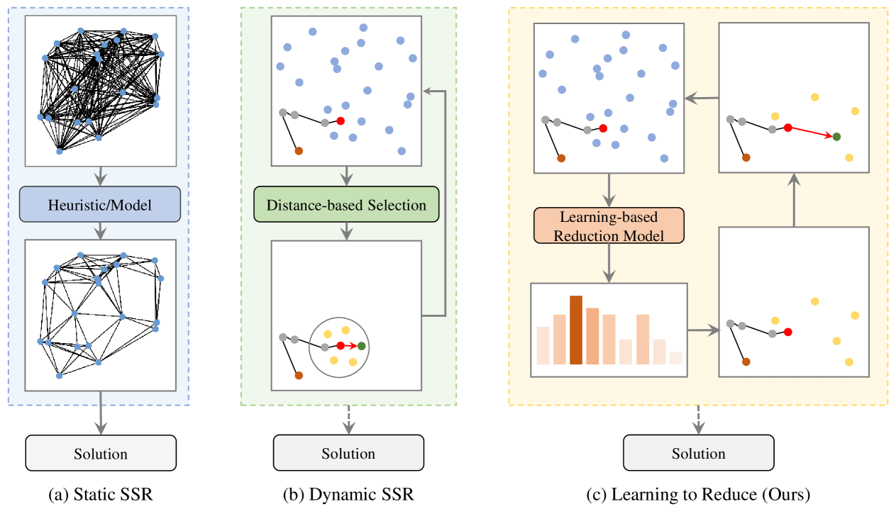
Figure 1: Different Search Space Reduction (SSR) Methods: (a) Static Search Space Reduction prunes the whole search space only once at the beginning of optimization process; (b) Dynamic Search Space Reduction reduces the search space to a small set of candidate nodes based on the distance to the last visited node at each construction step; (c) Learning to Reduce (Ours) builds reinforcement learning based model to adaptively reduce the search space and then select the next node for solution construction.

In recent years, neural combinatorial optimization (NCO) has emerged as a promising paradigm for solving complex problems like VRPs, which eliminates the need for time-consuming and handcrafted algorithm design by experts (Bengio et al., 2021; Li et al., 2022). These methods automatically learn problem-specific patterns through training frameworks such as supervised learning (SL) (Vinyals et al., 2015; Luo et al., 2023; Drakulic et al., 2023) or reinforcement learning (RL) (Bello et al., 2016; Kool et al., 2019; Zhou et al., 2024). A well-trained NCO model can directly construct approximate solutions without explicit search, offering a promising direction for real-time VRP solving. However, SL-based methods face a critical limitation due to the difficulty of obtaining high-quality labeled data (e.g., nearly optimal solutions) for large-scale NP-hard problems. In contrast, RL-based methods do not require labeled data and have demonstrated strong performance on small-scale instances (e.g., 100 nodes) (Kwon et al., 2020; Xin et al., 2021; Kim et al., 2022). Nevertheless, their effectiveness diminishes significantly on large-scale instances (e.g., 10,000 nodes), primarily due to the exponentially growing search space and the challenge of sparse reward.

To address the scalability challenges, search space reduction (SSR) has gained increasing attention as a scalable strategy. As listed in Table 1, existing SSR techniques can be broadly categorized into two types: static and dynamic. Static SSR performs a one-time pruning at the beginning of the optimization process, offering computational efficiency. However, it often requires additional search procedures (e.g., Monte Carlo Tree Search for TSP) to achieve high-quality solutions (Fu et al., 2021; Qiu et al., 2022; Sun & Yang, 2023). In contrast, dynamic SSR (Fang et al., 2024; Gao et al., 2024; Wang et al., 2024) adaptively adjusts the candidate node set at each construction step based on real-time problem states, enabling more effective search space reduction for constructive NCO methods. Despite their advantages, existing dynamic SSR methods are fundamentally constrained by their reliance on distance-based node selection, which struggle to generalize to large-scale instances, particularly those with non-uniform node distributions.

As shown in Figure 1, unlike existing SSR approaches, this work proposes a novel Learning to Reduce (L2R) framework for more flexible search space reduction that does not rely on the distance between nodes. Our contributions can be summarized as follows:

• We comprehensively analyze the key limitation of existing distance-based SSR methods and then propose a novel learning-based framework with hierarchical static and dynamic SSR for solving large-scale VRPs.

• In particular, we develop an RL-based approach to reduce search space and select candidate nodes at each construction step, significantly reducing computational overhead without compromising solution quality.

• We conduct comprehensive experiments to demonstrate that our proposed method, trained only on 100-node instances from uniform distribution, can generalize remarkably well to instances with up to 1 million nodes from uniform distribution and over 80k nodes from other distributions.

Table 1: Comparison between our L2R and classical neural vehicle routing solvers with search space reduction.

Neural Routing Solver	Static	Dynamic	Training	Generalizable
(Ordered by year of publication)	SSR	SSR	Scale	Scale
MLPR (Sun et al., 2021)	$\checkmark$	$\times$	$100$	2K
Att-GCN+MCTS (Fu et al., 2021)	$\checkmark$	$\times$	$50$	10K
DIMES (Qiu et al., 2022)	$\checkmark$	$\times$	10K	10K
DIFUSCO (Sun & Yang, 2023)	$\checkmark$	$\times$	10K	10K
T2T (Li et al., 2023)	$\checkmark$	$\times$	1K	1K
BQ (Drakulic et al., 2023)$\ddagger$	$\times$	Distance-based	$100$	1K
ELG (Gao et al., 2024)	$\times$	Distance-based	$100$	7K
DAR (Wang et al., 2024)	$\times$	Distance-based	$500$	11K
INViT (Fang et al., 2024)	$\times$	Distance-based	$100$	10K
L2R (Ours)	$\checkmark$	Learning-based	$100$	1M

• BQ (Drakulic et al., 2023) limits the sub-graph to the $250$ nearest neighbors of the current node when facing large-scale instances.

2 Related Work

2.1 NCO without Search Space Reduction

Most neural combinatorial optimization (NCO) models are trained on small-scale instances (e.g., 100 nodes) without search space reduction and achieve strong performance on instances of similar size. However, their effectiveness significantly diminishes when applied to larger instances (e.g., those exceeding 1,000 nodes) (Kool et al., 2019; Kwon et al., 2020). Some approaches incorporate additional search procedures, such as 2-opt (Deudon et al., 2018) and active search (Bello et al., 2016; Hottung et al., 2022), to address this limitation. While these techniques can improve solution quality, they are still computationally expensive for large-scale instances. Another line of research focuses on training NCO models directly on larger-scale instances (e.g., up to 500 nodes) to enhance generalization (Cao et al., 2021; Zhou et al., 2023, 2024). However, this approach incurs prohibitive computational costs due to the exponentially growing search space. Alternatively, some methods simplify large-scale VRPs through decomposition policies (Kim et al., 2021; Li et al., 2021; Hou et al., 2022; Pan et al., 2023; Zheng et al., 2024). Although effective, these methods often overlook the dependency between decomposition policies and subsequent solvers, resulting in suboptimal solutions. Moreover, the reliance on expert-designed policies limits their practicality for real-world applications.

2.2 NCO with Static Search Space Reduction

To address the scalability challenges of NCO methods, static search space reduction (SSR) has been proposed as a computationally efficient approach. These methods perform one-time pruning at the beginning of the optimization process, significantly reducing the problem size. For example, Sun et al. (2021) develop a static problem reduction technique to eliminate unpromising edges in large-scale TSP instances. Recently, heatmap-based approaches have gained popularity for solving large-scale TSPs, where models are trained to predict the probability of each edge belonging to the optimal solution. To handle large-scale instances, these methods often incorporate graph sparsification (Qiu et al., 2022; Sun & Yang, 2023; Li et al., 2023) or pruning strategies (Fu et al., 2021; Min et al., 2023) to reduce the search space. While static SSR is computationally efficient, it typically requires additional well-designed search procedures (e.g., Monte Carlo Tree Search for TSP) to achieve high-quality solutions, which might be more important for the optimization process (Xia et al., 2024).

2.3 NCO with Dynamic Search Space Reduction

Dynamic search space reduction (SSR) has also been explored as a promising approach to address the scalability challenges of NCO methods. These methods adaptively prune the search space to a small set of candidate nodes at each construction step, typically based on the distance to the last visited node. The final node selection can be guided by either the original policy augmented with auxiliary distance information (Wang et al., 2024) or a well-designed local policy (Gao et al., 2024). Additionally, recent work by Fang et al. (2024) and Drakulic et al. (2023) directly selects the next node from the candidate set using NCO models. While dynamic SSR can more efficiently reduce the search space for constructive NCO, its reliance on distance-based node selection is inappropriate for large-scale instances, especially those from non-uniform distributions.

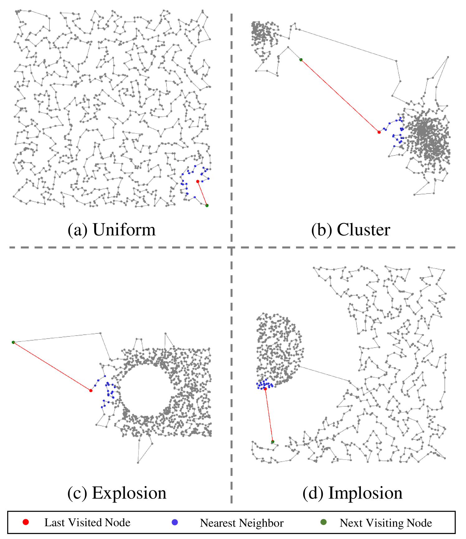
Figure 2: Impact of distance-based search space reduction on solution optimality. (a)-(d) Optimal solutions for TSP1000 instances under four distribution patterns: uniform, cluster, explosion, and implosion. Restricting the search space to the k-nearest neighbors (k = 20) will lead to suboptimal routes.

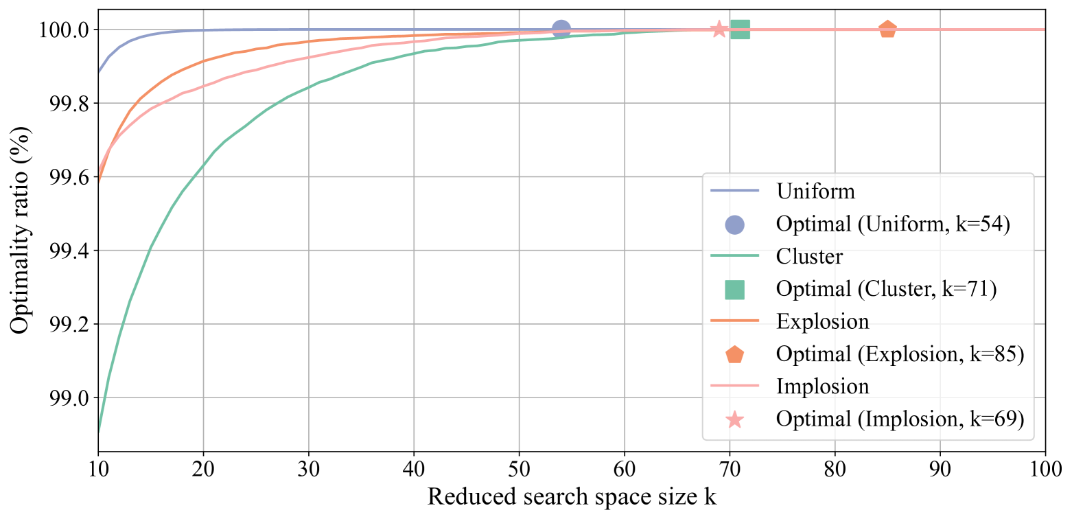
Figure 3: The effects of distance-based search space reduction on optimality ratio (TSP100).

3 Shortcomings of Distance-based Search Space Reduction

Constructive NCO methods solve routing problems by iteratively selecting nodes to build a solution. In theory, each step of this process should consider all unvisited nodes to guarantee optimality. However, for large-scale instances, this exponentially growing search space could quickly become computationally intractable. While current distance-based SSR methods can significantly improve computational efficiency, they also introduce critical limitations to NCO. In this section, we systematically analyze their shortcomings through two key perspectives: (1) the degradation of solution optimality and (2) the impact for the NCO solver.

Degradation of Solution Optimality

The fundamental limitation of distance-based search space reduction lies in its tendency to prune globally optimal nodes during sequential solution construction. As demonstrated in Figure 2, restricting candidate nodes to the $k$-nearest neighbors forces the algorithm to ignore critical long-range connections necessary for optimal routing. This over-pruning effect accumulates systematically across construction steps, ultimately compromising solution quality. The degradation is particularly severe in instances from non-uniform distributions, where optimal paths inherently rely on non-local node selections.

To quantify the impact of search space reduction size $k$ on solution optimality, we analyze the probability of retaining optimal nodes when restricting candidate selections to the $k$-nearest neighbors. For each of the four distributions (uniform, clustered, explosion, implosion), we generate 2,000 TSP100 instances and compute their optimal solutions using LKH3 (Helsgaun, 2017). We then measure the optimality ratio, defined as the proportion of construction steps where the optimal node resides within the $k$-nearest candidates.

As shown in Figure 3, the optimality ratio monotonically increases with $k$, and each distribution exhibits a critical threshold $k^{*}$ such that all optimal nodes are preserved when $k\geq k^{*}$. This implies that all nodes outside the $k^{*}$-nearest neighbors are redundant for optimal routing. However, when $k$ is small, the optimality ratio drops significantly. Moreover, a large $k^{*}$ indicates that search space reduction cannot significantly reduce the computational overhead, thereby failing to address the scalability challenge of solving large-scale routing problems.

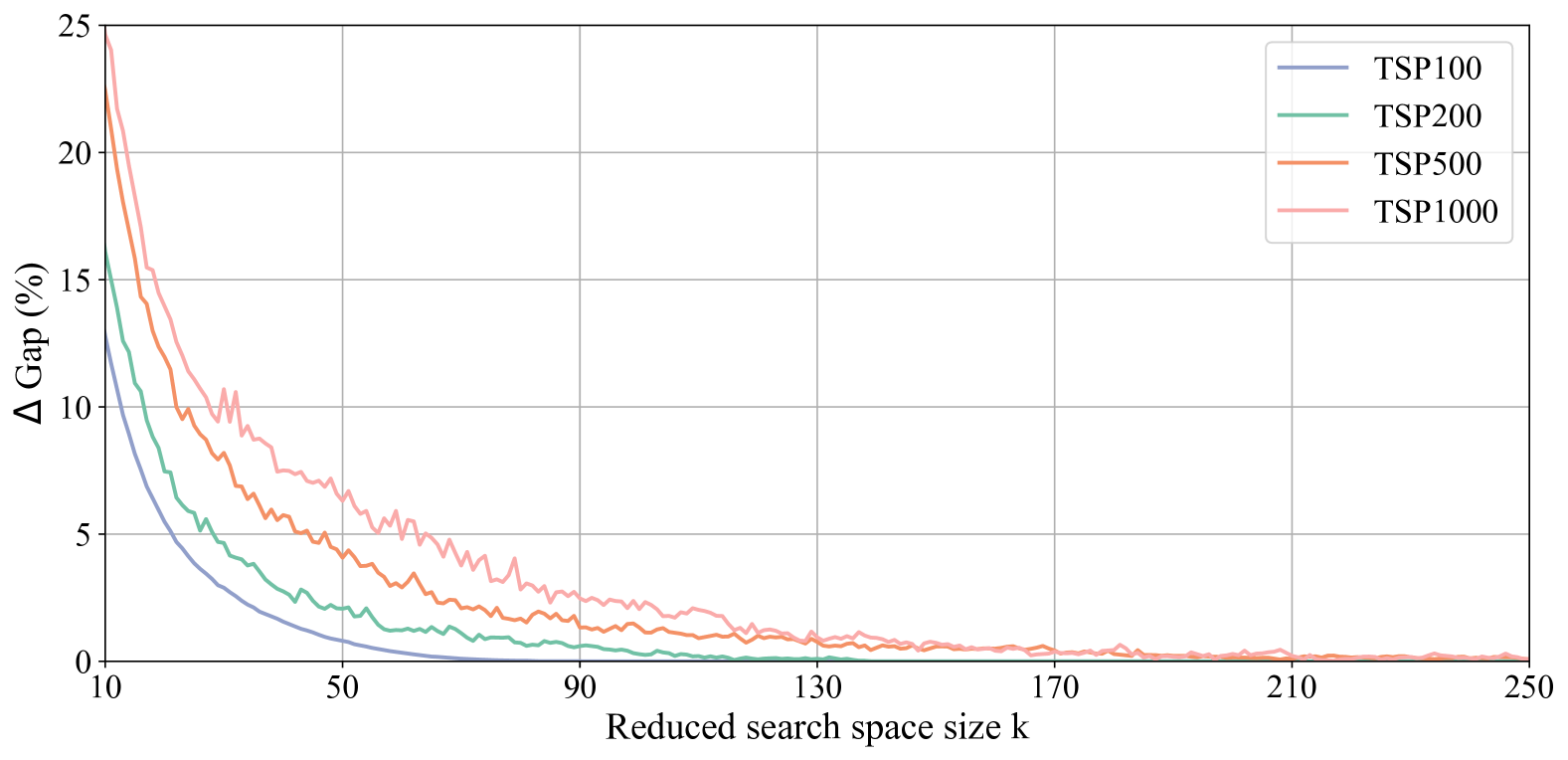
Figure 4: The effect of distance-based search space reduction on the gap in LEHD model (Luo et al., 2023). Here $\Delta Gap=Gap_{\text{reduced}}-Gap_{\text{original}}$.

Impact for Constructive NCO

To evaluate the impact of search space reduction on NCO performance, we use the well-known LEHD method (Luo et al., 2023) as a representative example, restricting the search space to the $k$ nearest nodes from the last visited node at each construction step. We quantify the impact by measuring the performance gap $\Delta Gap$, defined as the difference between the optimality gap obtained by LEHD with a reduced search space ($Gap_{\text{reduced}}$) and the original LEHD without search space reduction ($Gap_{\text{original}}$).

The results in Figure 4 illustrate the performance on TSP instances of varying sizes under different search space reduction levels ($k$). A key observation is the existence of a critical threshold $k^{*}$ for each problem size, beyond which LEHD with $k\geq k^{*}$ achieves a $0\%$ performance gap with the original LEHD, indicating no loss in solution quality with SSR. However, these critical thresholds vary significantly across problem sizes, and using a small $k<k^{*}$ leads to a substantial performance degradation. These findings highlight the potential of search space reduction while underscoring the need for advanced reduction methods capable of efficiently handling large-scale problems with a small $k$.

Figure 5: The pipeline of our proposed L2R framework for solving large-scale vehicle routing problem instances.

4 Learning to Reduce (L2R)

In this section, we propose Learning to Reduce (L2R), a hierarchical neural framework to address the scalability limitations of search space reduction in vehicle routing problems. As illustrated in Figure 5, our framework introduces three complementary stages: 1) static reduction, 2) learning-based reduction, and 3) local solution construction.

4.1 Static Reduction

The static reduction stage initiates our hierarchical framework by pruning the original fully connected graph $G=(V,E)$ into a sparse topology $G^{\prime}=(V,E^{\prime})$. For each node $v_{i}\in V$, we compute pairwise Euclidean distances $\{d_{ij}\}_{j=1}^{N}$ and eliminate connections to nodes in the farthest $\alpha$-percentile. Formally, the sparse edge set is defined as:

$$E^{\prime}=\bigcup_{v_{i}\in V}\left\{e_{ij}\mid\mathrm{rank}(d_{ij})\leq(1-\alpha)|V|\right\},\quad\alpha\in[0,1]$$ (1)

where $\mathrm{rank}(d_{ij})$ denotes the ascending order of distances from $v_{i}$ (i.e., $\mathrm{rank}(d_{ij})=1$ for the closest neighbor). Through empirical analysis across diverse scales and node distributions, we use $\alpha=10\%$ as the threshold in this work, which can efficiently reduce the computational overhead without compromising solution optimality. Crucially, this stage operates as a one-time preprocessing step, incurring no runtime overhead during subsequent solving phases.

4.2 Learning-based Reduction

The static reduction stage conducts partial search space pruning. However, there is still a large number of non-optimal edges remaining in the pruned graph $G^{\prime}$, which imposes prohibitive computational costs for NCO in large-scale scenarios. However, as discussed in the previous section, further distance-based search reduction with a large reduced rate will lead to a poor optimality ratio and poor performance.

To address this critical issue, we develop a learning-based model to dynamically evaluate the potential of feasible nodes and adaptively reduce the search space at each construction step. Our proposed model ensures efficiency through a lightweight structure containing only an embedding layer and an attention layer. Their implementations are detailed in the following.

Embedding Layer

Given an instance $S=\{\mathbf{s}_{i}\}_{i=1}^{N}$ with node features $\mathbf{s}_{i}\in\mathbb{R}^{d_{x}}$ (e.g., city coordinates in TSP), we first project these features into $d$-dimensional embeddings through a shared linear transformation for each node:

$$\mathbf{h}_{i}^{D}=W^{(e)}\mathbf{s}_{i}+\mathbf{b}^{(e)},\quad\forall i\in\{1,\dots,N\}$$ (2)

where $W^{(e)}\in\mathbb{R}^{d_{x}\times d}$ and $\mathbf{b}^{(e)}\in\mathbb{R}^{d}$ are learnable parameters. In other words, we obtain a set of embeddings $H^{D}=\{\mathbf{h}_{i}^{D}\}_{i=1}^{N}\in\mathbb{R}^{N\times d}$ for all nodes in the instance $S$.

At $t$-th step with partial solution $(\pi_{1},\dots,\pi_{\pi_{t-1}})$, we adopt the setting from Drakulic et al. (2023) to represent the current partial solution using the initial node embedding $\mathbf{h}_{\pi_{1}}^{D}$ and latest node embedding $\mathbf{h}_{\pi_{t-1}}^{D}$. In addition, following Kool et al. (2019) and Kwon et al. (2020), we define a context embedding of the current partial solution:

$$\mathbf{h}_{(C_{D})}^{t}=W_{\text{first}}\mathbf{h}_{\pi_{1}}^{D}+W_{\text{last}}\mathbf{h}_{\pi_{t-1}}^{D},$$ (3)

where $W_{\text{first}}\in\mathbb{R}^{d\times d}$ and $W_{\text{last}}\in\mathbb{R}^{d\times d}$ are two learnable matrices. In addition, we denote $\mathcal{A}_{t}$ as the set of all feasible nodes (e.g., unvisited cities with a valid edge in $E^{\prime}$ connected to the current city) at the $t$-th step. The embeddings of $\mathcal{A}_{t}$ are denoted by $H_{\mathcal{A}_{t}}^{D}=\{\mathbf{h}_{i}^{D}|i\in\mathcal{A}_{t}\}\in\mathbb{R}^{|\mathcal{A}_{t}|\times d}$.

Attention Layer

To calculate potential scores for all feasible nodes in $\mathcal{A}_{t}$, we process the context embedding $\mathbf{h}_{C_{D}}^{t}$ and node embeddings $H_{\mathcal{A}_{t}}^{D}$ through an attention mechanism. First, we project the node embeddings into key-value pairs:

$$K_{\mathcal{A}_{t}}^{D}=W^{K}H_{\mathcal{A}_{t}}^{D},\quad V_{\mathcal{A}_{t}}^{D}=W^{V}H_{\mathcal{A}_{t}}^{D}$$ (4)

where $W^{K},W^{V}\in\mathbb{R}^{d\times d}$ are learnable projection matrices. The context embedding then interacts with these projections through the attention operator:

$$\hat{\mathbf{h}}_{C_{D}}^{t}=\mathrm{Attention}\left(\mathbf{h}_{C_{D}}^{t},K_{\mathcal{A}_{t}}^{D},V_{\mathcal{A}_{t}}^{D}\right)$$ (5)

Finally, the potential scores $\{o_{i}|i\in\mathcal{A}_{t}\}\in\mathbb{R}^{1\times|\mathcal{A}_{t}|}$ can be computed as

$$o_{i}=\sigma\left(\frac{\hat{\mathbf{h}}_{(C_{D})}^{t}(W^{C}\mathbf{h}_{i}^{D})^{\mathrm{T}}}{\sqrt{d_{k}}}\right)-d_{t-1,i},\ \forall i\in\mathcal{A}_{t},$$ (6)

where $\sigma$ represents the Sigmoid function, $W^{C}\in\mathbb{R}^{d\times d}$ is a learnable parameter matrix, $d_{k}$ is the dimension for matrix $K_{\mathcal{A}_{t}}^{D}$, and $d_{t-1,i}$ denotes the distance between the current node $\pi_{t-1}$ and each feasible node $i$ with $i\in\mathcal{A}_{t}$, which is normalized into $[0,1]$ via division by $\sqrt{2}$ (i.e., the diagonal distance of unit square). Each score $o_{i}$ quantifies the potential of node $i\in\mathcal{A}_{t}$. Then we retain the top-$k$ nodes with highest potential scores as the candidate nodes and denote the set of all candidate nodes as $\mathcal{N}_{t}$. In this way, we have conducted a learning-based dynamic search space reduction at each construction step. More details can be found in Appendix A.

4.3 Local Solution Construction

In this subsection, we develop a learning-based local construction model to select one final node from the candidate set $\mathcal{N}_{t}$ to construct the partial solution at each step. Similar to previous work, we also use the initial node $\pi_{1}$ and the latest node $\pi_{t-1}$ to represent the current partial solution. First of all, the embedding of each node can be obtained by a shared linear transformation:

$$\mathbf{h}_{i}^{(0)}=W^{(0)}\mathbf{s}_{i}+\mathbf{b}^{(0)},\quad\forall i\in\{\pi_{1},\pi_{t-1}\}\cup\mathcal{N}_{t}$$ (7)

where $W^{(0)}$ and $b^{(0)}$ and learnable parameters. Then we can obtain the embedding of the partial graph:

$$\widetilde{H}^{(0)}=[W_{1}\mathbf{h}_{\pi_{1}}^{(0)},\ W_{2}\mathbf{h}_{\pi_{t-1}}^{(0)},\ H_{\mathcal{N}_{t}}^{(0)}]\in\mathbb{R}^{(2+|\mathcal{N}_{t}|)\times d}$$ (8)

where $[\cdot,\cdot]$ denotes the vertical concatenation operator, $H_{\mathcal{N}_{t}}^{(0)}=\{\mathbf{h}_{i}^{(0)}|i\in\mathcal{N}_{t}\}\in\mathbb{R}^{|\mathcal{N}_{t}|\times d}$ are the embeddings for all candidate nodes in $\mathcal{N}_{t}$, $W_{1}\in\mathbb{R}^{d\times d}$ and $W_{2}\in\mathbb{R}^{d\times d}$ are two learnable matrices. This embedding is the initial input to a sequence of attention layers.

In our proposed local construction model, one attention layer consists of two sub-layers: an attention sub-layer and a Feed-Forward (FF) sub-layer, both of which use Layer Normalization (Ba et al., 2016) and skip-connection (He et al., 2016). The detailed process can be found in Section B.3. After $L$ attention layers, the final embedding $\widetilde{H}^{(L)}=[\mathbf{h}_{\pi_{1}}^{(L)},\ \mathbf{h}_{\pi_{t-1}}^{(L)},\ H_{\mathcal{N}_{t}}^{(L)}]\in\mathbb{R}^{(2+|\mathcal{N}_{t}|)\times d}$ contains advanced feature representations of the initial, last, and $k$ candidate nodes.

Finally, similar to previous work (Kool et al., 2019; Kwon et al., 2020), we can compute the probabilities for selecting each node in $\mathcal{N}_{t}$ via a compatibility module:

$$u^{t}_{i}=\begin{cases}\xi\cdot\text{tanh}\left(\frac{\hat{\mathbf{h}}_{(C)}^{t}\left(\mathbf{h}_{i}^{(L)}\right)^{\mathrm{T}}}{\sqrt{d_{k}}}+a_{t-1,i}\right)&\text{if}\ i\in\mathcal{N}_{t}\\ -\infty&\text{otherwise}\end{cases},$$ (9)

where $\xi$ is the clipping parameter, $\hat{\mathbf{h}}_{(C)}^{t}=\mathbf{h}_{\pi_{1}}^{(L)}+\mathbf{h}_{\pi_{t-1}}^{(L)}$, and $a_{t-1,i}=f(|\mathcal{N}_{t}|,d_{t-1,i})$ represents the adaptation bias between each candidate node and the current node, following Zhou et al. (2024). The probability of selecting the $i$-th node as next visiting node can be calculated as

$$p_{\bm{\theta}}(\pi_{t}=i\mid S,\pi_{1:t-1})=\frac{e^{u_{i}^{t}}}{\sum_{j=1}^{|\mathcal{N}_{t}|}e^{u_{j}^{t}}}.$$ (10)

Thereby, the probability of generating a complete solution $\mathbf{\pi}$ for an instance $S$ can be calculated as

$$p_{\bm{\theta}}(\mathbf{\pi}\mid S)=\prod_{t=2}^{N}p_{\bm{\theta}}(\pi_{t}\mid S,\pi_{1:t-1}).$$ (11)

More details of local construction are in Appendix B.

4.4 Training

Our proposed L2R framework has a learning-based reduction model and a local construction model, which can be trained by a joint training scheme. We denote the learnable parameters as $\bm{\theta}_{R}$ and $\bm{\theta}_{L}$ for the reduction model and local construction model respectively, and hence $\bm{\theta}=\{\bm{\theta}_{R},\ \bm{\theta}_{L}\}$ contains all learnable parameters in the L2R framework.

Following Kool et al. (2019), L2R is trained by the REINFORCE (Williams, 1992) gradient estimator:

$$\nabla_{\bm{\theta}}\mathcal{L}(\bm{\theta}|S)=\mathbb{E}_{p_{\bm{\theta}}(\pi|S)}\left[\left(R(\pi|S)-b(S)\right)\nabla_{\bm{\theta}}\log p_{\bm{\theta}}(\pi|S)\right],$$ (12)

where $R(\pi\mid S)$ represents the total reward (e.g., the negative value of tour length) of instance $S$ given a specific solution $\pi$, and $b(S)$ is the greedy rollout baseline. The detailed training process are provided in Appendix D.

5 Experiments

In this section, we comprehensively evaluate our proposed model against classical and learning-based solvers on synthetic and real-world TSP and CVRP instances. Notably, our model is trained solely on 100-node TSP instances from uniform distribution. We assess its generalization performance on: (1) scalability to problem sizes up to 1 million nodes and (2) robustness to varying node distributions.

5.1 Experimental Setup

Problem Setting

For all problems, we generate synthetic instances following the methodology outlined in Kool et al. (2019). Specifically, we construct TSP test datasets with uniformly distributed nodes at six scales: 1K, 5K, 10K, 50K, 100K, and 1M. Following Fu et al. (2021), the TSP1K test set consists of 128 instances, while the larger TSP datasets each contain 16 instances. For the CVRP, we adhere to the capacity constraints specified in Hou et al. (2022) and generate five test datasets with scales of 1K, 5K, 7K, 10K, and 1M. Each dataset includes 100 instances, except for CVRP10K and CVRP1M, which contain 16 instances each.

The optimal solutions for the TSP and CVRP instances are obtained using LKH3 (Helsgaun, 2017) and HGS (Vidal, 2022), respectively. To evaluate cross-distribution generalization performance, we test on the TSP/CVRP5K instances from INViT (Fang et al., 2024). Additionally, we validate the real-world performance of L2R using symmetric EUC_2D instances from TSPLIB (Reinelt, 1991) and CVRPLIB Set-XXL (Arnold et al., 2019).

Table 2: Comparison on TSP instances with uniform distribution.

	TSP1K		TSP5K		TSP10K		TSP50K		TSP100K
Method	Obj. (Gap)	Time	Obj. (Gap)	Time	Obj. (Gap)	Time	Obj. (Gap)	Time	Obj. (Gap)	Time
LKH3	23.12 (0.00%)	1.7m	50.97 (0.00%)	12m	71.78 (0.00%)	33m	159.93 (0.00%)	10h	225.99 (0.00%)	25h
Concorde	23.12 (0.00%)	1m	50.95 (-0.05%)	31m	72.00 (0.15%)	1.4h	N/A	N/A	N/A	N/A
H-TSP	24.66 (6.66%)	48s	55.16 (8.21%)	1.2m	77.75 (8.38%)	2.2m	OOM		OOM
GLOP (more revisions)	23.78 (2.85%)	10.2s	53.15 (4.26%)	1.0m	75.04 (4.39%)	1.9m	168.09 (5.10%)	1.5m	237.61 (5.14%)	3.9m
LEHD greedy	23.84 (3.11%)	0.8s	58.85 (15.46%)	1.5m	91.33 (27.24%)	11.7m	OOM		OOM
LEHD RRC1,000	23.29 (0.72%)	3.3m	54.43 (6.79%)	8.6m	80.90 (12.5%)	18.6m	OOM		OOM
BQ greedy	23.65 (2.30%)	0.9s	58.27 (14.31%)	22.5s	89.73 (25.02%)	1.0m	OOM		OOM
BQ bs16	23.43 (1.37%)	13s	58.27 (10.7%)	24s	OOM		OOM		OOM
POMO aug$\times$8	32.51 (40.6%)	4.1s	87.72 (72.1%)	8.6m	OOM		OOM		OOM
ELG aug$\times$8	25.74 (11.33%)	0.8s	60.19 (18.08%)	21s	OOM		OOM		OOM
INViT-3V greedy	24.66 (6.66%)	9.0s	54.49 (6.90%)	1.2m	76.85 (7.07%)	3.7m	171.42 (7.18%)	1.3h	242.26 (7.20%)	5.0h
L2R greedy	24.14 (4.42%)	0.05s	53.33 (4.62%)	1.6s	75.16 (4.71%)	3.5s	167.65 (4.82% )	30s	236.60 (4.70%)	90.8s
L2R PRC100	23.61 (2.14%)	2.2s	52.34 (2.68%)	24s	73.86 (2.90%)	28s	165.02 (3.18% )	1.5m	234.10 (3.59%)	2.6m
L2R PRC500	23.51 (1.68%)	10.9s	52.19 (2.40%)	1.7m	73.61 (2.56%)	2.1m	164.37 (2.77% )	5.3m	232.89 (3.05%)	7.1m
L2R PRC1,000	23.49 (1.60%)	22s	52.15 (2.31%)	3.1m	73.56 (2.48%)	3.8m	164.22 (2.68% )	10.2m	232.49 (2.88%)	13m

Table 3: Comparison on CVRP instances following the setting in Hou et al. (2022).

	CVRP1K	CVRP5K	CVRP7K	CVRP10K
Method	Obj. (Time)	Obj. (Time)	Obj. (Time)	Obj. (Time)
HGS	41.2 (5m)	126.2 (5m)	172.1 (5m)	227.2 (5m)
L2D	46.3 (1.5s)	$-$	$-$	$-$
RBG	74.0 (13s)	$-$	$-$	$-$
TAM-AM*	50.1 (0.8s)	172.2 (12s)	233.4 (26s)	$-$
TAM-LKH3*	46.3 (1.8s)	144.6 (17s)	196.9 (33s)	$-$
TAM-HGS*	$-$	142.8 (30s)	193.6 (52s)	$-$
GLOP-G (LKH-3)	45.9 (1.1s)	140.6 (4.0s)	191.2 (5.8s)	256.4 (6.2s)
LEHD greedy	44.0 (0.8s)	138.2 (1.4m)	189.5 (3.8m)	257.3 (12m)
LEHD RRC1000	42.4 (3.4m)	132.7 (10m)	180.6 (19m)	$-$
BQ greedy	44.2 (1s)	139.9 (18.5s)	192.3 (42.2s)	262.2 (2m)
BQ bs16	43.1 (14s)	136.4 (2.4m)	186.8 (5.7m)	OOM
POMO aug$\times$8	101 (4.6s)	632.9 (11m)	OOM	OOM
ELG aug$\times$8	46.4 (10.3s)	OOM	OOM	OOM
INViT-3V greedy	48.2 (11s)	146.6 (1.4m)	197.6 (2.4m)	262.1 (4.3m)
L2R greedy	46.3 (0.1s)	137.2 (0.4s)	182.0 (0.7s)	238.1 (3.9s)
L2R PRC100	44.7 (3.6s)	133.2 (11.2s)	178.4 (15.5s)	235.2 (33.9s)
L2R PRC500	44.3 (17s)	131.7 (53.3s)	176.7 (1.2m)	233.2 (2.5m)
L2R PRC1,000	44.2 (34.2s)	131.1 (1.8m)	175.8 (2.5m)	232.3 (4.9m)

Table 4: Comparison on TSP instances with one million nodes.

	TSP1M			CVRP1M
Method†	Obj.	Gap	Time	Obj.	Gap	Time
Concorde/HGS	N/A	N/A	N/A	OOM
LKH3	713.97	0.00%	4.8h	N/A	N/A	N/A
POMO-SSR greedy	OOM			OOM
ELG-SSR greedy	OOM			OOM
INViT-3V greedy	N/A	N/A	N/A	N/A	N/A	N/A
L2R greedy	747.29	4.67%	33.67 m	17215.83	0.00%$\ddagger$	41.8m

• Except for INViT, which preserves the original neighborhood structure, other methods adopt D-SSR to align their search spaces with that of L2R.

• Because classical solvers (i.e., HGS and LKH3) fail to collect feasible solutions on CVRP1M, the gap reported for CVRP1M is measured relative to the best-obtained solution.

Model & Training Setting

For all experiments, we use an embedding dimension of $128$ and a feed-forward layer dimension of $512$. To enhance geometric pattern recognition in VRPs, we integrate scale and distance information into the attention mechanism (see Appendix C for implementation details). The local construction model employs $6$ attention layers. Consistent with Kool et al. (2019), we set the clipping parameter $\xi=10$ in Equation 9. The hyperparameter $k$ is configured as $20$ for TSP and $50$ for CVRP. All experiments are conducted on a single NVIDIA GeForce RTX 3090 GPU (24GB memory).

Our model is exclusively trained on uniform-distributed instances with $100$ nodes. We employ the Adam optimizer (Kingma & Ba, 2014) with an initial learning rate of $\eta=10^{-4}$ and a learning rate decay of $0.98$ per epoch. Training spans $100$ epochs with $2\text{,}500$ batches per epoch. Due to memory constraints, batch sizes differ across problems—$180$ for TSP and $64$ for CVRP. Identical model configurations are maintained across all experiments. Additional implementation details are provided in Appendix D (training setting) and Appendix E (model setting).

Baseline

We compare L2R with the following methods: (1) Classical Solver: Concorde (Applegate et al., 2006), LKH3 (Helsgaun, 2017), HGS (Vidal, 2022); (2) Constructive NCO: POMO (Kwon et al., 2020), Omni_VRP (Zhou et al., 2023), ELG (Gao et al., 2024), BQ (Drakulic et al., 2023), LEHD (Luo et al., 2023), and INViT (Fang et al., 2024); (3) Two-Stage NCO: TAM (Hou et al., 2022), L2D (Li et al., 2021), RBG (Zong et al., 2022), H-TSP (Pan et al., 2023), and GLOP (Ye et al., 2024).

Metrics and Inference

We report the average objective value (Obj.), optimality gap (Gap), and average inference time (Time) for each method. The optimality gap quantifies the discrepancy between the solutions generated by the corresponding methods and the optimal solutions. It is important to note that the inference time for classical solvers, which run on a single CPU, and for learning-based methods, which utilize GPUs, are inherently different. Therefore, these times should not be directly compared.

For most NCO baseline methods, we execute the source code provided by the authors using default settings. Results marked with an asterisk (*) are directly obtained from the corresponding papers. Some methods fail to produce feasible solutions within a reasonable time limit (e.g., several days), which is denoted by ‘N/A’. The notation ‘OOM’ indicates that the memory consumption exceeds the available memory limits. For L2R, we report two types of results—those obtained by greedy trajectory (greedy) and those derived from Parallel local ReConstruction (PRC) under different numbers of iterations (Luo et al., 2024). The parallel approach demonstrates promising results by effectively trading computing time for improved solution quality. For PRC, the initial solutions are generated using the greedy trajectory. PRC100 refers to $100$ iterations, with the longest destruction length per iteration set to $1\text{,}000$ to balance speed and effectiveness. Further details about PRC are available in Luo et al. (2024).

Table 5: Comparison on cross-distribution generalization.

	TSP5K, Cluster		TSP5K, Explosion		TSP5K, Implosion
Method	Obj. (Gap)	Time	Obj. (Gap)	Time	Obj. (Gap)	Time
LKH3	28.84 (0.00%)	$-$	31.98 (0.00%)	$-$	45.04 (0.00%)	$-$
ELG	35.42 (22.83%)	1.6m	38.60 (20.71%)	1.6m	52.95 (17.55%)	1.6m
Omni_VRP	44.56 (54.53%)	1.1m	48.32 (51.09%)	1.1m	67.66 (50.20%)	1.1m
INViT-3V greedy	31.32 (8.60%)	1.3m	35.68 (11.59%)	1.3m	48 87 (8.49%)	1.3m
L2R greedy	30.44 (5.56%)	1.4s	34.79 (8.78%)	1.3s	47.77 (6.06%)	1.4s
L2R PRC1,000	29.66 (2.87%)	2.3m	33.13 (3.61%)	2.3m	46.26(2.71%)	2.3m
	CVRP5K, Cluster		CVRP5K, Explosion		CVRP5K, Implosion
Method	Obj. (Gap)	Time	Obj. (Gap)	Time	Obj. (Gap)	Time
HGS	472.44 (0.00%)	$-$	350.82 (0.00%)	$-$	582.70 (0.00%)	$-$
ELG	558.13 (18.14%)	2.4m	397.18 (13.21%)	2.2m	626.37 (7.50%)	2.2m
Omni_VRP	576.62 (22.05%)	1.3m	466.92 (33.09%)	1.4m	816.94 (40.20%)	1.3m
INViT-3V greedy	514.97 (9.00%)	1.6m	381.14 (8.64%)	1.6m	637.03 (9.32%)	1.6m
L2R greedy	486.24 (2.92%)	1.6s	366.98 (4.61%)	1.6s	606.19 (4.03%)	1.6s
L2R PRC1,000	480.12 (1.63%)	3.5m	357.61 (1.94%)	3.5m	591.61 (1.53%)	3.5m

• All datasets and optimal solutions are obtained from INViT(Fang et al., 2024) and each contains $20$ instances. Note that for CVRP instances, the capacity is unified at $50$.

• The instance augmentation technique is not employed to prevent methods from exceeding memory limits.

Table 6: Comparison on large-scale TSPLIB (Reinelt, 1991) instances ($1,000\leq N\leq 85,900$) and CVRPLIB Set-XXL (Arnold et al., 2019) ($3,000\leq N\leq 30,000$).

Method	1K $\leq N\leq$ 5K	5K <$N\leq$ 100K	All	Solved#
	(23 instances)	(10 instances)	(33 instances)
BQ bs16	10.65%	30.58%†	$-$	26/33
LEHD greedy	11.14%	39.34%†	$-$	30/33
ELG aug$\times$8	11.34%	OOM	$-$	23/33
INViT-3V greedy	11.49%	10.00%	11.04%	33/33
L2R greedy	9.50%	7.23%	8.81%	33/33
Method	3K <$N\leq$ 7K	7K <$N\leq$ 30K	All	Solved#
	(4 instances)	(6 instances)	(10 instances)
BQ bs16	20.20%	OOM	$-$	4/10
LEHD greedy	22.22%	32.80%†	$-$	6/10
ELG aug$\times$8	16.82% †	OOM	$-$	2/10
INViT-3V greedy	20.74%	26.64%	24.28%	10/10
L2R greedy	13.36%	11.58%	12.29%	10/10

• Some instances are skipped due to the OOM issue.

• The RRC and PRC techniques are not employed due to computational efficiency.

5.2 Performance Evaluation

VRPs with Uniform Distribution

We conduct experiments on large-scale routing instances with uniform distribution, and the experimental results are reported in Table 2 (TSP1K$-$TSP100K), Table 3 (CVRP1K$-$CVRP10K), and Table 4 (TSP/CVRP1M). Benefiting from an efficient search space reduction scheme, our method consistently delivers superior inference performance across various problem instances. While it does not surpass SL-based LEHD and BQ on TSP/CVRP1K, our proposed L2R achieves significantly shorter runtime compared to other methods, such as LEHD (e.g., $22\ \text{sec}$ vs. $3\ \text{min}$ on $128$ TSP1K instances). For larger-scale instances, the superiority of L2R becomes increasingly pronounced. To the best of our knowledge, L2R is the first neural solver capable of effectively solving TSP and CVRP instances with one million nodes. Compared to classic heuristic methods, L2R achieves a $4.67\%$ optimality gap and an $8\times$ speed-up over LKH-3 on $16$ TSP1M instances. Additionally, L2R successfully tackles CVRP1M instances that exceed the computational limits of both LKH3 and HGS.

Cross-Distribution VRPs

We evaluate L2R’s cross-distribution performance on TSP5K/CVRP5K instances from three distinct distributions: cluster, explosion, and implosion. As shown in Table 5, L2R consistently achieves the best performance among all comparable methods across these distributions. These results further highlight L2R’s robust generalization capabilities.

Benchmark Dataset

We further assess L2R’s generalization performance on instances from CVRPLIB Set-XXL (Arnold et al., 2019) and TSPLIB (Reinelt, 1991). As demonstrated in Table 6, L2R maintains its position as the best-performing model across instances of varying scales, underscoring its practical applicability in real-world scenarios. Detailed results are provided in Appendix F.

5.3 Ablation Study

Effects of Learning-based Reduction

To validate the effectiveness of learning-based reduction in L2R, we train a new model using dynamic distance-based SSR while keeping all other settings unchanged. The results demonstrate that L2R consistently outperforms this alternative with dynamic SSR, particularly in solving cross-distribution instances. Detailed results are provided in Section G.1.

L2R vs. Distance-based SSR with Larger Search Space

We train three dynamic distance-based SSR models with varying search space sizes ($k=50,75,100$) and compare them with our proposed L2R model ($k=20$) on TSP instances of different problem sizes. The results show that L2R, despite its smaller search space, consistently outperforms the distance-based SSR models with larger search spaces across instances of varying scales. Detailed results are available in Section G.2.

6 Conclusion

In this work, we propose a novel RL-based Learning-to-Reduce (L2R) framework for solving large-scale vehicle routing problems. Our approach adaptively selects a small set of candidate nodes at each construction step, enabling efficient search space reduction while maintaining solution quality. Extensive experiments demonstrate that L2R, trained exclusively on 100-node instances from the uniform distribution, achieves remarkable performance on TSP and CVRP instances with up to 1 million nodes from uniform distribution and over 80K nodes from other distributions.

Impact Statement

This paper presents work whose goal is to advance the field of Machine Learning. There are many potential societal consequences of our work, none of which we feel must be specifically highlighted here.

Appendix A Learning-based Reduction Model for CVRPs

We develop a learning-based reduction model to dynamically evaluate the potential of feasible nodes and adaptively reduce the search space at each construction step. Our proposed model ensures efficiency through a lightweight architecture consisting of only an embedding layer and an attention layer. For CVRPs, we introduce a specialized treatment for each node to address the unique demands of the problem. In this section, we provide a detailed description of this specialized treatment for CVRPs in the reduction model.

Embedding Layer

Given an instance $S=\{\mathbf{s}_{i}\}_{i=1}^{N+1}$ with node features $\mathbf{s}_{i}\in\mathbb{R}^{d_{x}}$ (i.e., node coordinates and demand), we separate the depot and nodes and feed them into distinct linear layers. The detailed calculation is expressed as

$$\mathbf{h}_{i}^{D}=\begin{cases}W_{\text{depot}}^{(e)}[x_{i},\ y_{i}]+\mathbf{b}_{\text{depot}}^{(e)},&i=0\\ W_{\text{node}}^{(e)}[x_{i},\ y_{i},\ \delta_{i}]+\mathbf{b}_{\text{node}}^{(e)},&i=1,\dots,N\end{cases},$$ (13)

where $x_{i}$ and $y_{i}$ denote the node coordinates, $\delta_{i}$ is the demand of node $i$, $W_{\text{depot}}^{(e)}\in\mathbb{R}^{2\times d}$ and $\mathbf{b}_{\text{depot}}^{(e)}\in\mathbb{R}^{d}$ are learnable parameters for the depot, and $W_{\text{node}}^{(e)}\in\mathbb{R}^{3\times d}$ and $\mathbf{b}_{\text{node}}^{(e)}\in\mathbb{R}^{d}$ are learnable parameters for the nodes. This process yields a set of embeddings $H^{D}=\{\mathbf{h}_{i}^{D}\}_{i=1}^{N+1}$ for all nodes in the instance $S$.

At the $t$-th step, with a partial solution following Kool et al. (2019) and Kwon et al. (2020), we define a context embedding for the current partial solution:

$$\mathbf{h}_{(C_{D})}^{t}=W_{\text{last}}[\mathbf{h}_{\pi_{t-1}}^{D},Q_{\text{remain}}],$$ (14)

where $W_{\text{last}}\in\mathbb{R}^{(1+d)\times d}$ is a learnable matrix, and $Q_{\text{remain}}$ represents the current remaining capacity.

Masking

The static reduction stage performs partial search space reduction to obtain the pruned graph $G^{\prime}$. In particular, we do not allow nodes to be visited if their remaining demand is either $0$ (indicating the node has already been visited) or exceeds the remaining capacity of the vehicle. We denote $\mathcal{A}_{t}$ as the set of all feasible nodes, and the embeddings of $\mathcal{A}_{t}$ are represented by $H_{\mathcal{A}_{t}}^{D}=\{\mathbf{h}_{i}^{D}\mid i\in\mathcal{A}_{t}\}\in\mathbb{R}^{|\mathcal{A}_{t}|\times d}$.

Appendix B Local Solution Construction Model

The proposed local solution construction model includes four components: 1) coordinate normalization, 2) embedding layer, 3) attention layer, and 4) compatibility calculation, which are detailed in the following subsections.

B.1 Coordinate Normalization

We introduce a coordinate normalization operation to ensure that each extracted sub-graph $G_{\text{sub}}^{{}^{\prime}}$ adheres to a similar distribution (Fu et al., 2021; Ye et al., 2024; Fang et al., 2024). This operation not only simplifies the input feature space but also significantly enhances the stability and homogeneity of model inputs across different sub-graphs. Following Fu et al. (2021) and Fang et al. (2024), the coordinate transformation is formulated as

$$x^{\text{min}} ={\min_{i\in\mathcal{N}_{t}}x_{i}},\quad x^{\text{max}}={\max_{i\in\mathcal{N}_{t}}x_{i}},$$ (15)

$$y^{\text{min}} ={\min_{i\in\mathcal{N}_{t}}y_{i}},\quad y^{\text{max}}={\max_{i\in\mathcal{N}_{t}}y_{i}},$$

$$r=\frac{1}{\max(x^{\text{max}}-x^{\text{min}},y^{\text{max}}-y^{\text{min}})},$$ (16)

$$x_{i}^{new} =r\times(x_{i}-x^{\text{min}})\quad\forall i\in\{\pi_{1},\pi_{t-1}\}\cup\mathcal{N}_{t},$$ (17)

$$y_{i}^{new} =r\times(y_{i}-y^{\text{min}})\quad\forall i\in\{\pi_{1},\pi_{t-1}\}\cup\mathcal{N}_{t},$$

where $x_{i}$ and $y_{i}$ denote the node coordinates, and $\mathcal{N}_{t}$ represents the $k$ candidate nodes generated based on $\pi_{t-1}$ and the dynamic reduction model. To ensure that the first visited node (or depot) $\pi_{1}$ remains within the boundary (i.e., $0\leq x_{i}^{new}\leq 1$), we apply $x_{i}^{new}=\max(0,\min(x_{i}^{new},1))$, and the same operation is applied to $y_{i}^{new}$. Equations (15)–(17) effectively simplify the input feature space and improve the stability and homogeneity of model inputs across different sub-graphs. Subsequently, the sub-graph $G_{\text{sub}}^{{}^{\prime}}$ is transformed into a new graph $G_{\text{sub}}^{{}^{\prime\prime}}$.

B.2 Embedding Layer

Traveling Salesman Problem

Given the converted sub-graph $G_{\text{sub}}^{{}^{\prime\prime}}$, the embedding layer first transforms the coordinates into initial embeddings using a shared linear layer with learnable parameters $[W^{(0)}\in\mathbb{R}^{d_{x}\times d};b^{(0)}\in\mathbb{R}^{d}]$. The embeddings of the $k$ candidate nodes $\mathcal{N}_{t}$ are denoted by $H_{\mathcal{N}}^{(0)}=\{\mathbf{h}_{i}^{(0)}\mid i\in\mathcal{N}_{t}\}\in\mathbb{R}^{k\times d}$. Here, the first node $\pi_{1}$ and the last node $\pi_{t-1}$ are used to represent the current partial solution. Therefore, their initial embeddings require special treatment (Drakulic et al., 2023; Luo et al., 2023). Specifically, additional learnable matrices $W_{1}\in\mathbb{R}^{d\times d}$ and $W_{2}\in\mathbb{R}^{d\times d}$ are applied to $\mathbf{h}_{\pi_{1}}^{(0)}$ and $\mathbf{h}_{\pi_{t-1}}^{(0)}$, respectively. Accordingly, we define the initial graph node embeddings $\widetilde{H}^{(0)}\in\mathbb{R}^{(2+|\mathcal{N}_{t}|)\times d}$ as

$$\widetilde{H}^{(0)}=[W_{1}\mathbf{h}_{\pi_{1}}^{(0)},\ W_{2}\mathbf{h}_{\pi_{t-1}}^{(0)},\ H_{\mathcal{N}_{t}}^{(0)}],$$ (18)

where $[\cdot,\cdot]$ denotes the vertical concatenation operator. Next, $\widetilde{H}^{(0)}$ is passed through the $L$ attention layers sequentially.

Capacitated Vehicle Routing Problem

For CVRP, due to the demands and capacity constraints, we introduce a specialized treatment for the initial embedding of each node. Specifically, the node demands are normalized as $\delta_{i}=\{\delta/Q_{\text{remain}}\mid i\in\mathcal{N}_{t}\}$, where $Q_{\text{remain}}$ represents the remaining capacity. We separate the coordinates and demands and feed them into distinct linear layers. The detailed calculation is expressed as

$$\mathbf{h}_{i_{\text{coor}}}^{(0)} =W^{(0)}[x_{i},y_{i}]+\mathbf{b}^{(0)}\quad\forall i\in\{\pi_{1},\pi_{t-1}\}\cup\mathcal{N}_{t},$$ (19)

$$\mathbf{h}_{i}^{(0)} =\mathbf{h}_{i_{\text{coor}}}^{(0)}+W_{\text{demand}}\delta_{i}\quad\forall i\in\mathcal{N}_{t},$$

$$\mathbf{h}_{\pi_{1}}^{(0)} =W_{1}\mathbf{h}_{{\pi_{1}}_{\text{coor}}}^{(0)}+W_{\text{load}}Q_{\text{remain}},$$

$$\mathbf{h}_{\pi_{t-1}}^{(0)} =W_{2}\mathbf{h}_{{\pi_{t-1}}_{\text{coor}}}^{(0)}+W_{\text{load}}Q_{\text{remain}},$$

where $W_{\text{demand}}\in\mathbb{R}^{1\times d}$ and $W_{\text{load}}\in\mathbb{R}^{1\times d}$ are learnable matrices used for demand and remaining capacity, respectively.

B.3 Attention Layer

Inspired by BQ (Drakulic et al., 2023) and LEHD (Luo et al., 2023), our attention layer adopts a heavy decoder structure and consists of two sub-layers: an attention sub-layer and a feed-forward (FF) sub-layer. Both sub-layers incorporate layer normalization (Ba et al., 2016) and skip connections (He et al., 2016).

Let $\widetilde{H}^{(\ell-1)}=[\mathbf{h}_{\pi_{1}}^{(\ell-1)},\ \mathbf{h}_{\pi_{t-1}}^{(\ell-1)},\ H_{\mathcal{N}_{t}}^{(\ell-1)}]$ denote the input to the $\ell$-th attention layer for $\ell=1,\ldots,L$. The outputs for the $i$-th node are computed as follows:

$$\hat{\mathbf{h}}_{i}^{(\ell)}=\mathrm{LN}^{(\ell)}\left(\mathbf{h}_{i}^{(\ell-1)}+\mathrm{Attention}^{(\ell)}\left(\mathbf{h}_{i}^{(\ell-1)},\widetilde{H}^{(\ell-1)}\right)\right),$$ (20)

$$\mathbf{h}_{i}^{(\ell)}=\mathrm{LN}^{(\ell)}\left(\mathbf{\hat{h}}_{i}^{(\ell)}+\mathrm{FF}^{(\ell)}\left(\mathbf{\hat{h}}_{i}^{(\ell)}\right)\right),$$ (21)

where $\mathrm{LN}(\cdot)$ denotes layer normalization (Ba et al., 2016), which mitigates potential value overflows caused by exponential operations; $\mathrm{Attention}$ in Equation 20 represents the adopted attention mechanism (see Appendix C for details); and $\mathrm{FF}(\cdot)$ in Equation 21 corresponds to a fully connected neural network with ReLU activation.

After $L$ attention layers, the final node embeddings $\widetilde{H}^{(L)}=[\mathbf{h}_{\pi_{1}}^{(L)},\ \mathbf{h}_{\pi_{t-1}}^{(L)},\ H_{\mathcal{N}_{t}}^{(L)}]\in\mathbb{R}^{(2+|\mathcal{N}_{t}|)\times d}$ encapsulate the advanced feature representations of the first node, last node, and $k$ candidate nodes.

B.4 Padding

To address the variability in the number of candidate nodes when solving a batch of instances, we pad the number of candidate nodes $|\mathcal{N}_{t}|$ to the maximum length by adding an all-zero tensor. The maximum length is computed as $\max\{\min\{k,|\mathcal{A}_{i,t}|\}\mid i\in\{1,\dots,B\}\}$, where $k$ is the predefined search space size, $|\mathcal{A}_{i,t}|$ denotes the number of feasible unvisited nodes at the current step $t$ for instance $S_{i}$, and $B$ represents the batch size. An attention mask is then applied to mask out the padded zeros during computation.

Appendix C Adaptation Attention Free Module

Following Zhou et al. (2024), we implement $\mathrm{Attention}(\cdot)$ using a scale-distance Adaptation Attention Free Module (AAFM) to enhance geometric pattern recognition for routing problems. Given the input $X$, AAFM first transforms it into $Q$, $K$, and $V$ through corresponding linear projection operations:

$$Q=XW^{Q},\quad K=XW^{K},\quad V=XW^{V},$$ (22)

where $W^{Q}$, $W^{K}$, and $W^{V}$ are learnable matrices. The AAFM computation is then expressed as:

$$\mathrm{Attention}=\sigma(Q)\odot\frac{\exp(A)(\exp(K)\odot V)}{\exp(A)\exp(K)},$$ (23)

where $\sigma$ denotes the sigmoid function, $\odot$ represents the element-wise product, and $A=\{\mathbf{a}_{ij}\}$ denotes the pair-wise adaptation bias, it is calculated as:

$$a_{ij}=-\alpha\cdot\log_{2}N\cdot d_{ij}\quad\forall i,j\in\{1,\ldots,N\},$$ (24)

where $N$ is the total number of nodes, $d_{ij}$ represents the distance between node $i$ and node $j$, and $\alpha>0$ is a learnable parameter with a default value of 1. Compared to multi-head attention (MHA) (Vaswani et al., 2017), AAFM enables the model to explicitly capture instance-specific knowledge by updating pair-wise adaptation biases while exhibiting lower computational overhead. Further details are provided in the related work section mentioned above.

Appendix D Training

Following Kool et al. (2019), we employ an exponential baseline ($\beta=0.8$) during the first epoch to stabilize initial learning. The baseline parameters $\bm{\theta}^{BL}$ are updated only if the improvement is statistically significant, as determined by a paired t-test ($\alpha=5\%$) conducted on $10\text{,}000$ separate evaluation instances at the end of each epoch. If the baseline policy is updated, new evaluation instances are sampled to prevent overfitting. Additionally, at the first construction step for TSP, $\pi_{1}$ is randomly selected as the initial partial solution and is treated as both the first and last nodes for subsequent decoding steps.

Algorithm 1 L2R Training with REINFORCE Algorithm

1: Input: number of epochs $E$, steps per epoch $T$, batch size $B$, significance $\alpha$,

2: Output: The trained model with parameters $\bm{\theta}=\{\bm{\theta}_{R},\bm{\theta}_{L}\}$, which are reduction model $\bm{\theta}_{R}$ and local construction model $\bm{\theta}_{L}$

3: Init $\bm{\theta}_{R},\ \bm{\theta}_{R}^{BL}\leftarrow\bm{\theta}_{R}$ and $\bm{\theta}_{L},\ \bm{\theta}_{L}^{BL}\leftarrow\bm{\theta}_{L}$

4: for $\text{epoch}=1,\ldots,E$ do

5:  for $\text{step}=1,\ldots,T$ do

6:   $G_{i}\leftarrow\text{RandomInstance()}\enspace\forall i\in\{1,\ldots,B\}$

7:   $G_{i}^{{}^{\prime}}\leftarrow\text{StaticReduction()}\enspace\forall i\in\{1,\ldots,B\}$

8:   while not done do

9:    // $\mathcal{N}_{i,t}$ denotes the $k$ high-potential candidate nodes at step $t$ given sparse graph $G_{i}^{{}^{\prime}}$

10:    $\mathcal{N}_{i,t}\leftarrow$ DynamicReduction($G_{i}^{{}^{\prime}},\ \pi_{t-1}$, $\bm{\theta}_{R}$) $\enspace\forall i\in\{1,\ldots,B\}$

11:    // using a decoding strategy of sampling according to the output probabilities

12:    $\pi_{i,t}\leftarrow$ LocalConstruction($\pi_{1},\ \pi_{t-1},\ \mathcal{N}_{i,t}$, $\bm{\theta}_{L}$) $\enspace\forall i\in\{1,\ldots,B\}$

13:   end while

14:   while not done do

15:    // $\mathcal{N}_{i,t}^{BL}$ denotes the $k$ high-potential candidate nodes at step $t$ given sparse graph $G_{i}^{{}^{\prime}}$

16:    $\mathcal{N}_{i,t}^{BL}\leftarrow$ DynamicReduction($G_{i}^{{}^{\prime}},\ \pi_{t-1}^{BL}$, $\bm{\theta}_{R}^{BL}$) $\enspace\forall i\in\{1,\ldots,B\}$

17:    // using a decoding strategy of greedy according to the output probabilities

18:    $\pi_{i,t}^{BL}\leftarrow$ LocalConstruction($\pi_{1}^{BL},\ \pi_{t-1}^{BL},\ \mathcal{N}_{i,t}^{BL}$, $\bm{\theta}_{L}^{BL}$) $\enspace\forall i\in\{1,\ldots,B\}$

19:   end while

20:   $\nabla\mathcal{L}\leftarrow\sum_{i=1}^{B}\left(R(\bm{\pi}_{i})-R(\bm{\pi}_{i}^{BL})\right)\nabla_{\bm{\theta}}\log p_{\bm{\theta}}(\bm{\pi}_{i})$

21:   $\bm{\theta}\leftarrow\text{Adam}(\bm{\theta},\nabla\mathcal{L})$

22:  end for

23:  if $\text{OneSidedPairedTTest}(p_{\bm{\theta}},p_{\bm{\theta}^{\text{BL}}})<\alpha$ then

24:   $\bm{\theta}_{R}^{BL}\leftarrow\bm{\theta}_{R}$

25:   $\bm{\theta}_{L}^{BL}\leftarrow\bm{\theta}_{L}$

26:  end if

27: end for

Appendix E Model Setting

Detailed information about the hyperparameter settings can be found in Table 7. Here, the number of layers denotes the number of attention layers of the local construction model.

Table 7: Model hyperparameter settings in experiments.

Hyperparameter	TSP	CVRP
Optimizer	Adam
Initial learning rate	$10^{-4}$
Learning rate decay	$0.98$ per epoch
The number of attention layer	$6$
Embedding dimension	$128$
Feed forward dimension	$512$
Clipping parameter	10
Training capacity	$-$	$50$
Maximum search space size $k$	$20$	$50$
Percentage of static reduction	$10\%$
Gradient clipping	max_norm=$1.0$
Weight decay	$-$
Batch size	$180$	$64$
Batches of each epoch	$2,500$
Training scale	$100$
Epochs	$100$

Appendix F Detailed Results on Real-world Datasets

We evaluate the generalization performance on instances from CVRPLIB Set-XXL (Arnold et al., 2019) and TSPLIB (Reinelt, 1991). Detailed results for large-scale instances are provided in Table 8 and Table 9. The results demonstrate that L2R consistently outperforms other models across instances of varying scales, demonstrating its strong applicability in real-world scenarios.

Table 8: The detailed results on large-scale TSPLIB (Reinelt, 1991) instances ($5,000\leq N\leq 85,900$).

Instance	Scale	BQ	LEHD	ELG	INViT	L2R
		bs16	greedy	aug$\times$8	greedy	greedy
rl5915	5,915	19.58%	24.17%	OOM	14.02%	7.57%
rl5934	5,934	24.53%	24.11%	OOM	12.91%	12.63%
pla7397	7,397	47.63%	40.94%	OOM	9.45%	7.59%
rl11849	11,849	OOM	38.04%	OOM	12.71%	7.93%
usa13509	13,509	OOM	71.10%	OOM	13.44%	7.46%
brd14051	14,051	OOM	41.22%	OOM	9.31%	6.53%
d15112	15,112	OOM	35.82%	OOM	7.24%	6.60%
d18512	18,512	OOM	OOM	OOM	6.62%	5.23%
pla33810	33,810	OOM	OOM	OOM	7.04%	6.13%
pla85900	85,900	OOM	OOM	OOM	7.21%	4.62%
Sloved#		3/10	7/10	0/10	10/10	10/10
Avg.gap		30.58%†	39.34%†	$-$	10.00%	7.23%

• Some instances are skipped due to the OOM issue.

Table 9: The detailed results on CVRPLIB XXL (Arnold et al., 2019) instances ($3,000\leq N\leq 30,000$).

Instance	Scale	BQ	LEHD	ELG	INViT	L2R
		bs16	greedy	aug$\times$8	greedy	greedy
Leuven1	3,000	15.39%	16.60%	12.12%	13.71%	11.53%
Leuven2	4,000	25.69%	34.85%	21.52%	26.08%	16.14%
Antwerp1	6,000	13.64%	14.66%	OOM	15.40%	13.14%
Antwerp2	7,000	26.09%	22.77%	OOM	27.75%	12.63%
Ghent1	10,000	OOM	27.23%	OOM	15.87%	10.29%
Ghent2	11,000	OOM	38.36%	OOM	30.78%	12.78%
Brussels1	15,000	OOM	OOM	OOM	18.09%	12.93%
Brussels2	16,000	OOM	OOM	OOM	32.08%	12.61%
Flanders1	20,000	OOM	OOM	OOM	23.41%	7.81%
Flanders2	30,000	OOM	OOM	OOM	39.60%	13.05%
Sloved#		4/10	6/10	2/10	10/10	10/10
Avg.gap		20.20%†	25.75%†	16.82%†	24.28%	12.29%

• Some instances are skipped due to the OOM issue.

Appendix G Ablation Study

G.1 Effects of Learning-based Reduction

Table 10: Comparison between different reduction approaches on cross-distribution generalization with $5,000$ nodes. D-SSR denotes distance-based search space reduction.

Method	Uniform	Cluster	Explosion	Implosion
LKH3	0.00%	0.00%	0.00%	0.00%
D-SSR ($k=20$)	5.04%	5.73%	9.54%	6.20%
L2R ($k=20$)	4.62%	5.56%	8.78%	6.06%

G.2 L2R vs. Distance-based SSR with Larger Search Space

Table 11: Comparison between learning-based small space and distance-based large space on TSP instances with uniform distribution. D-SSR denotes distance-based search space reduction.

Method	TSP1K	TSP5K	TSP10K	TSP50K	TSP100K
LKH3	0.00%	0.00%	0.00%	0.00%	0.00%
D-SSR ($k=50$)	5.51%	6.30%	6.73%	6.52%	6.62%
D-SSR ($k=75$)	5.13%	6.23%	6.95%	7.15%	7.33%
D-SSR ($k=100$)	4.50%	5.20%	5.39%	5.63%	5.74%
L2R ($k=20$)	4.42%	4.62%	4.71%	4.82%	4.70%

Appendix H Solution Visualizations

H.1 Solution Visualizations of Cross-distribution TSP Instances

(a) Optimal solution.

(b) L2R with greedy decoding (gap: 4.28%).

Figure 6: The solution visualizations of a TSP5K instance with uniform distribution.

(a) Optimal solution.

(b) L2R with greedy decoding (gap: 4.59%).

Figure 7: The solution visualizations of a TSP5K instance with cluster distribution.

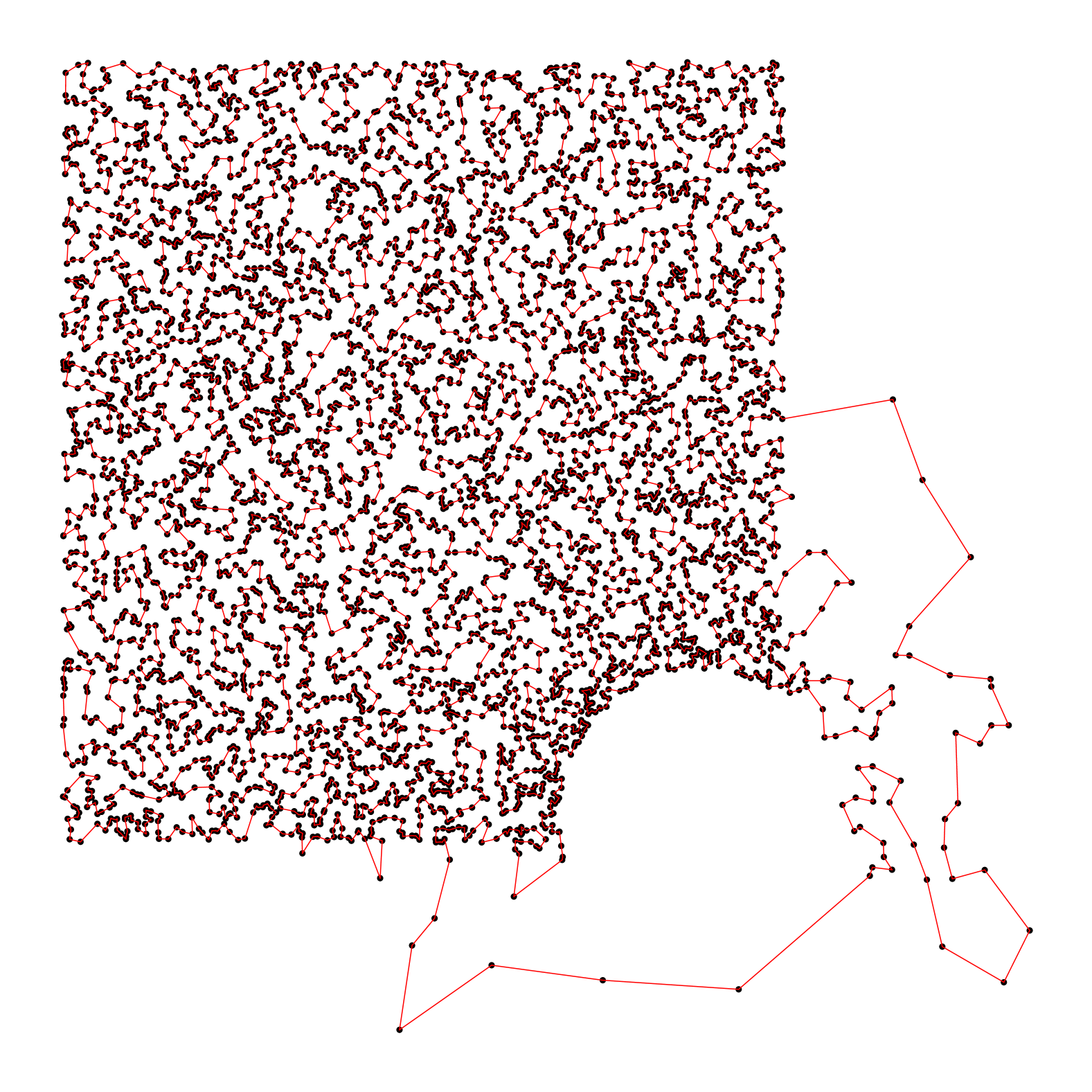
(a) Optimal solution.

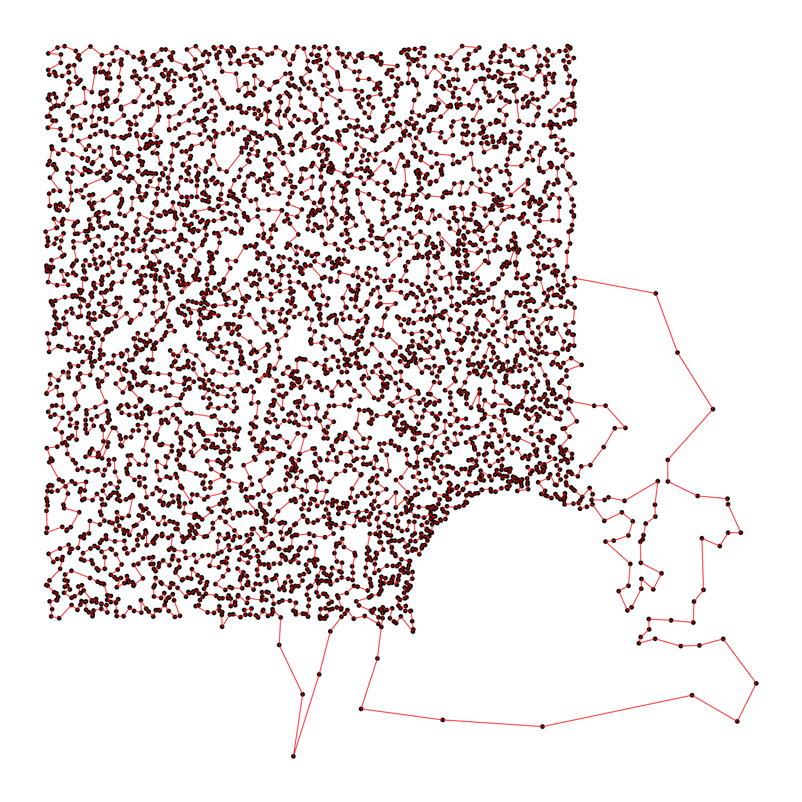
(b) L2R with greedy decoding (gap: 4.39%).

Figure 8: The solution visualizations of a TSP5K instance with explosion distribution.

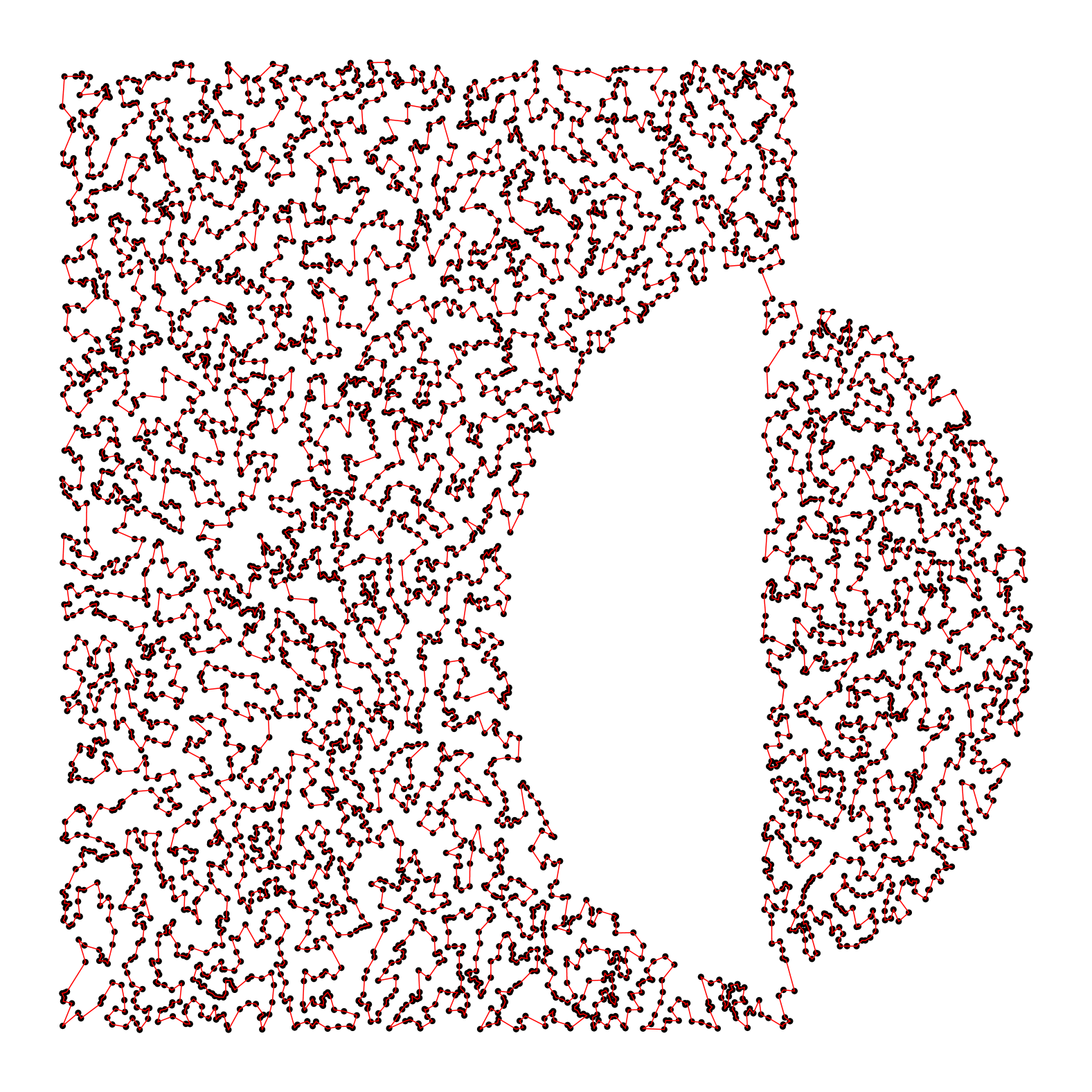
(a) Optimal solution.

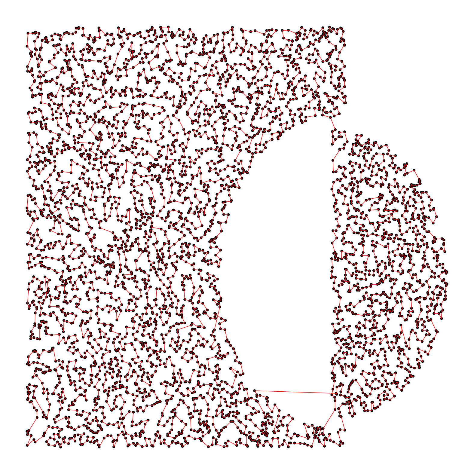
(b) L2R with greedy decoding (gap: 4.47%).

Figure 9: The solution visualizations of a TSP5K instance with implosion distribution.

H.2 Solution Visualizations of Large-scale TSPLIB Instances

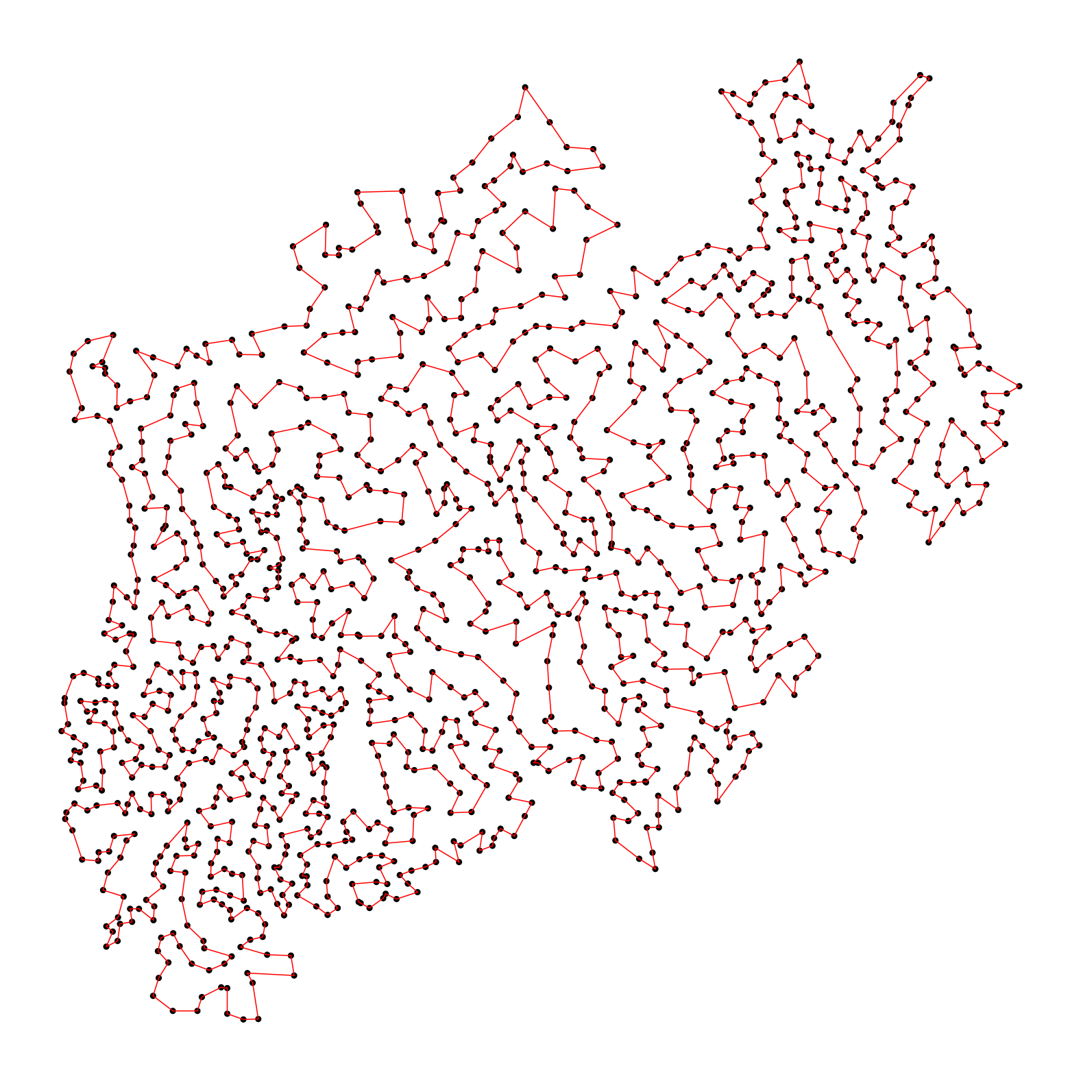
(a) Instance nrw1379 (scale: 1379, gap: 3.39%).

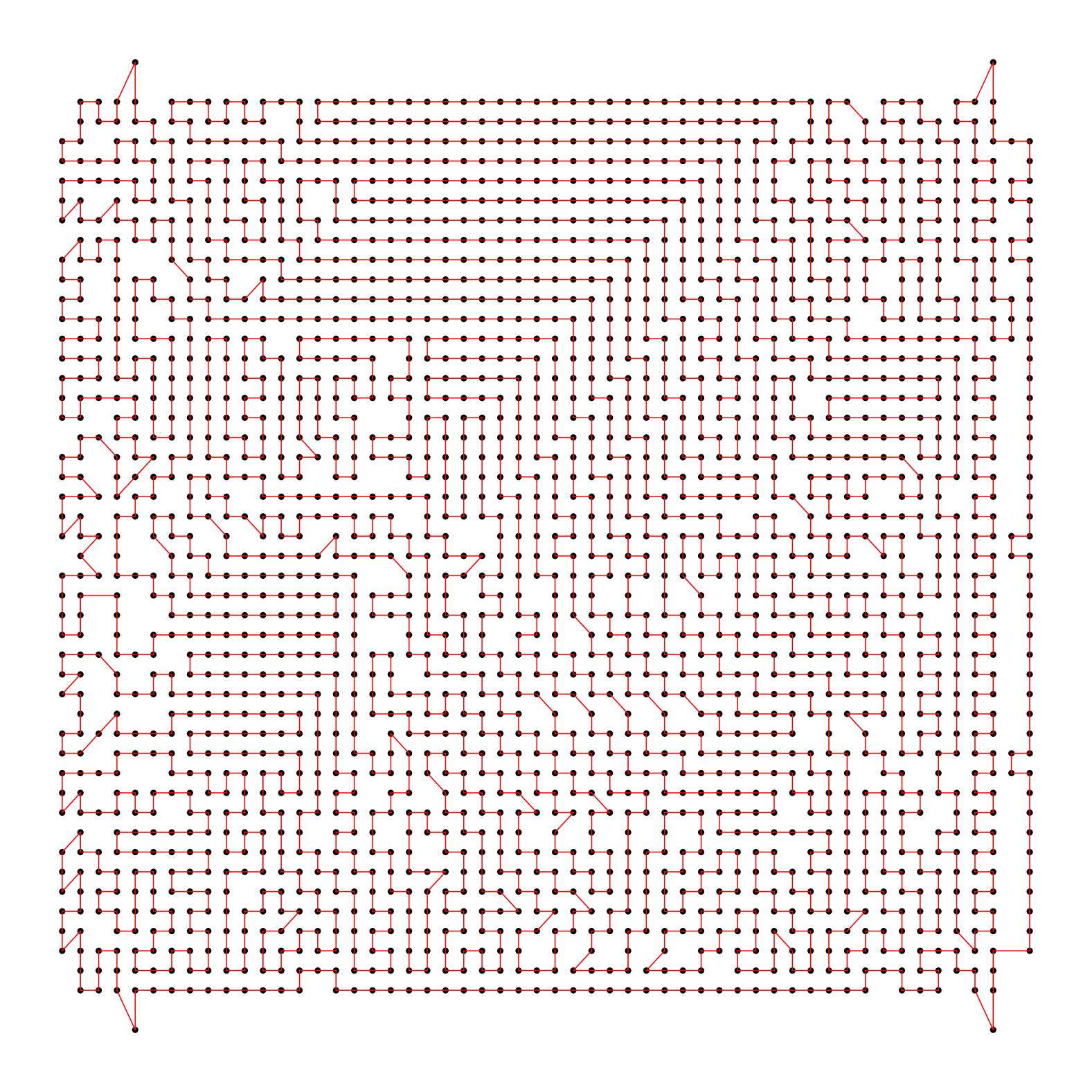
(b) Instance u2319 (scale: 2319, gap: 0.43%).

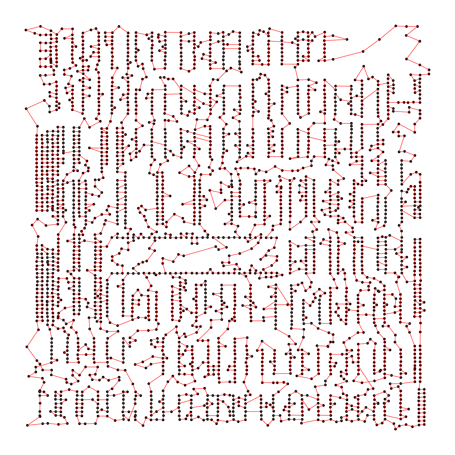
(c) Instance pcb3038 (scale: 3038, gap: 4.89%).

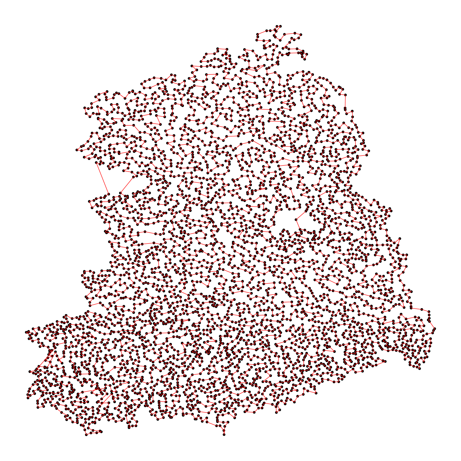
(d) Instance fnl4461 (scale: 4461, gap: 4.28%).

Figure 10: The solution visualizations of TSPLIB (Reinelt, 1991) instances with different scales, the solutions are all generated by L2R with greedy decoding.

Appendix I Licenses for Used Resources

Table 12: List of licenses for the codes and datasets we used in this work

Resource	Type	Link	License
Concorde (Applegate et al., 2006)	Code	https://github.com/jvkersch/pyconcorde	BSD 3-Clause License
LKH3 (Helsgaun, 2017)	Code	http://webhotel4.ruc.dk/~keld/research/LKH-3/	Available for academic research use
HGS (Vidal, 2022)	Code	https://github.com/chkwon/PyHygese	MIT License
L2D (Li et al., 2021)	Code	https://github.com/mit-wu-lab/learning-to-delegate	Available for academic research use
H-TSP (Pan et al., 2023)	Code	https://github.com/Learning4Optimization-HUST/H-TSP	Available for academic research use
GLOP (Ye et al., 2024)	Code	https://github.com/henry-yeh/GLOP	MIT License
POMO (Kwon et al., 2020)	Code	https://github.com/yd-kwon/POMO/tree/master/NEW_py_ver	MIT License
ELG (Gao et al., 2024)	Code	https://github.com/gaocrr/ELG	MIT License
Omni_VRP (Zhou et al., 2023)	Code	https://github.com/RoyalSkye/Omni-VRP	MIT License
INViT (Fang et al., 2024)	Code	https://github.com/Kasumigaoka-Utaha/INViT	Available for academic research use
LEHD (Luo et al., 2023)	Code	https://github.com/CIAM-Group/NCO_code/tree/main/single_objective/LEHD	Available for any non-commercial use
BQ (Drakulic et al., 2023)	Code	https://github.com/naver/bq-nco	CC BY-NC-SA 4.0 license
Cross-distribution TSPs(Fang et al., 2024)	Dataset	https://github.com/Kasumigaoka-Utaha/INViT	MIT License
Cross-distribution CVRPs(Fang et al., 2024)	Dataset	https://github.com/Kasumigaoka-Utaha/INViT	MIT License
TSPLIB (Reinelt, 1991)	Dataset	http://comopt.ifi.uni-heidelberg.de/software/TSPLIB95/	Available for any non-commercial use
CVRPLIB Set-XXL (Arnold et al., 2019)	Dataset	http://vrp.galgos.inf.puc-rio.br/index.php/en/	Available for academic research use

We list the used existing codes and datasets in Table 12, and all of them are open-sourced resources for academic usage.

References

- Applegate et al. (2006) Applegate, D., Bixby, R., Chvatal, V., and Cook, W. Concorde tsp solver, 2006.
- Arnold et al. (2019) Arnold, F., Gendreau, M., and Sörensen, K. Efficiently solving very large-scale routing problems. Computers & operations research, 107:32–42, 2019.
- Ba et al. (2016) Ba, J. L., Kiros, J. R., and Hinton, G. E. Layer normalization. arXiv preprint arXiv:1607.06450, 2016.
- Bello et al. (2016) Bello, I., Pham, H., Le, Q. V., Norouzi, M., and Bengio, S. Neural combinatorial optimization with reinforcement learning. arXiv preprint arXiv:1611.09940, 2016.
- Bengio et al. (2021) Bengio, Y., Lodi, A., and Prouvost, A. Machine learning for combinatorial optimization: a methodological tour d’horizon. European Journal of Operational Research, 290(2):405–421, 2021.
- Cao et al. (2021) Cao, Y., Sun, Z., and Sartoretti, G. Dan: Decentralized attention-based neural network for the minmax multiple traveling salesman problem. arXiv preprint arXiv:2109.04205, 2021.
- Deudon et al. (2018) Deudon, M., Cournut, P., Lacoste, A., Adulyasak, Y., and Rousseau, L.-M. Learning heuristics for the tsp by policy gradient. In Integration of Constraint Programming, Artificial Intelligence, and Operations Research: 15th International Conference, CPAIOR 2018, Delft, The Netherlands, June 26–29, 2018, Proceedings 15, pp. 170–181. Springer, 2018.
- Drakulic et al. (2023) Drakulic, D., Michel, S., Mai, F., Sors, A., and Andreoli, J.-M. Bq-nco: Bisimulation quotienting for efficient neural combinatorial optimization. In Thirty-seventh Conference on Neural Information Processing Systems, 2023.
- Fang et al. (2024) Fang, H., Song, Z., Weng, P., and Ban, Y. Invit: A generalizable routing problem solver with invariant nested view transformer. In International Conference on Machine Learning, 2024.
- Fu et al. (2021) Fu, Z.-H., Qiu, K.-B., and Zha, H. Generalize a small pre-trained model to arbitrarily large tsp instances. In Proceedings of the AAAI Conference on Artificial Intelligence, volume 35, pp. 7474–7482, 2021.
- Gao et al. (2024) Gao, C., Shang, H., Xue, K., Li, D., and Qian, C. Towards generalizable neural solvers for vehicle routing problems via ensemble with transferrable local policy. In International Joint Conference on Artificial Intelligence, 2024.
- He et al. (2016) He, K., Zhang, X., Ren, S., and Sun, J. Deep residual learning for image recognition. In Proceedings of the IEEE Conference on Computer Vision and Pattern Recognition, pp. 770–778, 2016.
- Helsgaun (2017) Helsgaun, K. An extension of the lin-kernighan-helsgaun tsp solver for constrained traveling salesman and vehicle routing problems. Roskilde: Roskilde University, 12, 2017.
- Hottung et al. (2022) Hottung, A., Kwon, Y.-D., and Tierney, K. Efficient active search for combinatorial optimization problems. In International Conference on Learning Representations, 2022.
- Hou et al. (2022) Hou, Q., Yang, J., Su, Y., Wang, X., and Deng, Y. Generalize learned heuristics to solve large-scale vehicle routing problems in real-time. In The Eleventh International Conference on Learning Representations, 2022.
- Kim et al. (2021) Kim, M., Park, J., et al. Learning collaborative policies to solve np-hard routing problems. Advances in Neural Information Processing Systems, 34:10418–10430, 2021.
- Kim et al. (2022) Kim, M., Park, J., and Park, J. Sym-nco: Leveraging symmetricity for neural combinatorial optimization. Advances in Neural Information Processing Systems, 35:1936–1949, 2022.
- Kingma & Ba (2014) Kingma, D. P. and Ba, J. Adam: A method for stochastic optimization. arXiv preprint arXiv:1412.6980, 2014.
- Kool et al. (2019) Kool, W., van Hoof, H., and Welling, M. Attention, learn to solve routing problems! In International Conference on Learning Representations, 2019.
- Kwon et al. (2020) Kwon, Y.-D., Choo, J., Kim, B., Yoon, I., Gwon, Y., and Min, S. Pomo: Policy optimization with multiple optima for reinforcement learning. Advances in Neural Information Processing Systems, 33:21188–21198, 2020.
- Li et al. (2022) Li, B., Wu, G., He, Y., Fan, M., and Pedrycz, W. An overview and experimental study of learning-based optimization algorithms for the vehicle routing problem. IEEE/CAA Journal of Automatica Sinica, 9(7):1115–1138, 2022.
- Li et al. (2021) Li, S., Yan, Z., and Wu, C. Learning to delegate for large-scale vehicle routing. Advances in Neural Information Processing Systems, 34:26198–26211, 2021.
- Li et al. (2023) Li, Y., Guo, J., Wang, R., and Yan, J. T2t: From distribution learning in training to gradient search in testing for combinatorial optimization. In Thirty-seventh Conference on Neural Information Processing Systems, 2023.
- Luo et al. (2023) Luo, F., Lin, X., Liu, F., Zhang, Q., and Wang, Z. Neural combinatorial optimization with heavy decoder: Toward large scale generalization. In Thirty-seventh Conference on Neural Information Processing Systems, 2023.
- Luo et al. (2024) Luo, F., Lin, X., Wang, Z., Tong, X., Yuan, M., and Zhang, Q. Self-improved learning for scalable neural combinatorial optimization. arXiv preprint arXiv:2403.19561, 2024.
- Min et al. (2023) Min, Y., Bai, Y., and Gomes, C. P. Unsupervised learning for solving the travelling salesman problem. Advances in Neural Information Processing Systems, 36, 2023.
- Pan et al. (2023) Pan, X., Jin, Y., Ding, Y., Feng, M., Zhao, L., Song, L., and Bian, J. H-tsp: Hierarchically solving the large-scale travelling salesman problem. In Proceedings of the AAAI Conference on Artificial Intelligence, 2023.
- Qiu et al. (2022) Qiu, R., Sun, Z., and Yang, Y. Dimes: A differentiable meta solver for combinatorial optimization problems. Advances in Neural Information Processing Systems, 35:25531–25546, 2022.
- Reinelt (1991) Reinelt, G. Tsplib—a traveling salesman problem library. ORSA Journal on Computing, 3(4):376–384, 1991.
- Sar & Ghadimi (2023) Sar, K. and Ghadimi, P. A systematic literature review of the vehicle routing problem in reverse logistics operations. Computers & Industrial Engineering, 177:109011, 2023.
- Sun et al. (2021) Sun, Y., Ernst, A., Li, X., and Weiner, J. Generalization of machine learning for problem reduction: a case study on travelling salesman problems. Or Spectrum, 43(3):607–633, 2021.
- Sun & Yang (2023) Sun, Z. and Yang, Y. Difusco: Graph-based diffusion solvers for combinatorial optimization. Advances in Neural Information Processing Systems, 36:3706–3731, 2023.
- Tiwari & Sharma (2023) Tiwari, K. V. and Sharma, S. K. An optimization model for vehicle routing problem in last-mile delivery. Expert Systems with Applications, 222:119789, 2023.
- Vaswani et al. (2017) Vaswani, A., Shazeer, N., Parmar, N., Uszkoreit, J., Jones, L., Gomez, A. N., Kaiser, Ł., and Polosukhin, I. Attention is all you need. Advances in Neural Information Processing Systems, 30, 2017.
- Vidal (2022) Vidal, T. Hybrid genetic search for the cvrp: Open-source implementation and swap* neighborhood. Computers & Operations Research, 140:105643, 2022.
- Vinyals et al. (2015) Vinyals, O., Fortunato, M., and Jaitly, N. Pointer networks. Advances in Neural Information Processing Systems, 28, 2015.
- Wang et al. (2024) Wang, Y., Jia, Y.-H., Chen, W.-N., and Mei, Y. Distance-aware attention reshaping: Enhance generalization of neural solver for large-scale vehicle routing problems. arXiv preprint arXiv:2401.06979, 2024.
- Williams (1992) Williams, R. J. Simple statistical gradient-following algorithms for connectionist reinforcement learning. Machine Learning, 8:229–256, 1992.
- Xia et al. (2024) Xia, Y., Yang, X., Liu, Z., Liu, Z., Song, L., and Bian, J. Position: Rethinking post-hoc search-based neural approaches for solving large-scale traveling salesman problems. arXiv preprint arXiv:2406.03503, 2024.
- Xin et al. (2021) Xin, L., Song, W., Cao, Z., and Zhang, J. Multi-decoder attention model with embedding glimpse for solving vehicle routing problems. In Proceedings of the AAAI Conference on Artificial Intelligence, volume 35, pp. 12042–12049, 2021.
- Ye et al. (2024) Ye, H., Wang, J., Liang, H., Cao, Z., Li, Y., and Li, F. Glop: Learning global partition and local construction for solving large-scale routing problems in real-time. In Proceedings of the AAAI Conference on Artificial Intelligence, volume 38, pp. 20284–20292, 2024.
- Zheng et al. (2024) Zheng, Z., Zhou, C., Xialiang, T., Yuan, M., and Wang, Z. Udc: A unified neural divide-and-conquer framework for large-scale combinatorial optimization problems. In Thirty-eighth Conference on Neural Information Processing Systems, 2024.
- Zhou et al. (2024) Zhou, C., Lin, X., Wang, Z., Tong, X., Yuan, M., and Zhang, Q. Instance-conditioned adaptation for large-scale generalization of neural combinatorial optimization. arXiv preprint arXiv:2405.01906, 2024.
- Zhou et al. (2023) Zhou, J., Wu, Y., Song, W., Cao, Z., and Zhang, J. Towards omni-generalizable neural methods for vehicle routing problems. In International Conference on Machine Learning, 2023.
- Zong et al. (2022) Zong, Z., Wang, H., Wang, J., Zheng, M., and Li, Y. Rbg: Hierarchically solving large-scale routing problems in logistic systems via reinforcement learning. In Proceedings of the 28th ACM SIGKDD Conference on Knowledge Discovery and Data Mining, pp. 4648–4658, 2022.