Controlling tissue size by active fracture

Abstract

Groups of cells, including clusters of cancerous cells, multicellular organisms, and developing organs, may both grow and break apart. What physical factors control these fractures? In these processes, what sets the eventual size of clusters? We develop a framework for understanding cell clusters that can fragment due to cell motility using an active particle model. We compute analytically how the break rate of cell-cell junctions depends on cell speed, cell persistence, and cell-cell junction properties. Next, we find the cluster size distributions, which differ depending on whether all cells can divide or only the cells on the edge of the cluster divide. Cluster size distributions depend solely on the ratio of the break rate to the growth rate—allowing us to predict how cluster size and variability depend on cell motility and cell-cell mechanics. Our results suggest that organisms can achieve better size control when cell division is restricted to the cluster boundaries or when fracture can be localized to the cluster center. Our results link the general physics problem of a collective active escape over a barrier to size control, providing a quantitative measure of how motility can regulate organ or organism size.

How does an organ or an organism control its size? Size is thought to be tightly regulated by feedbacks controlling cell division [1]. However, two recent experiments suggest a different possibility—that the size of a group of cells can arise from a competition between growth, which tends to make the group larger, and random cell motility, which can make the group fracture into multiple pieces, reducing group size. In the metazoan Trichoplax adhaerens, asexual reproduction by fission is driven by motility-induced fractures [2]. Similarly, germline cysts in mice are formed by a combination of cell division and fracture of intercellular bridges by random cell motility [3]. These mechanisms are more reminiscent of how cancerous cells can break from an invading front [4, 5, 6] than a well-regulated organism. Can motility-driven fracture reliably regulate the size of a group of cells? Both T. adhaerens and germline cysts show significant variability in size [2, 3]. What physical factors control the group size and its variability?

We argue that the size of cell clusters controlled by fracture is set by competition between the break rate of cell-cell junctions $k_{b}$ and the cell division rate $k_{d}$. We model break rate $k_{b}$ from a mechanical perspective, using a simple one-dimensional model of cells as active particles connected by springs. The break rate depends on typical cell speed, cell-cell junction strength, and the cell’s persistence time. We then develop models of cluster growth and fracture. We derive the exact steady-state cluster size distribution, finding that cluster sizes depend solely on the ratio $k_{b}/k_{d}$, allowing us to link cluster size to cell adhesion and motility. The quality of cluster size control can be improved if only cells on the edge of the cluster divide or if only cell-cell junctions near the cluster middle can fracture.

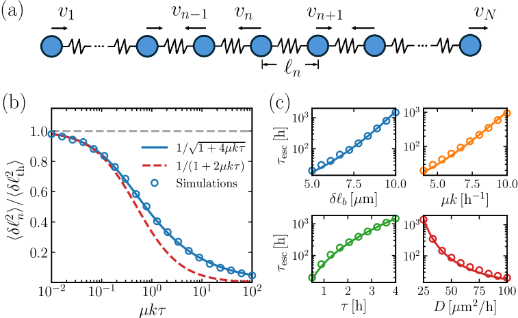
Figure 1: (a) Illustration of the active chain model. Cells are connected by springs; each cell has active velocity $v_{n}$. (b) Variance of the spring stretch $\langle\delta\ell_{n}^{2}\rangle$ as a function of $\mu k\tau$. Gray dashed line is the thermal variance $\langle\delta\ell^{2}_{\mathrm{th}}\rangle=D/\mu k$. We change $\mu k\tau$ by varying $\tau$ while fixing $\mu k$ in the simulations. Red dashed line is the two-particle result $\langle\delta\ell^{2}\rangle_{2}$. (c) Mean escape time $\tau_{\mathrm{esc}}=1/k_{b}$. Empty circles are simulation results with $N=1000$ cells; solid lines are theory, Eq. (4).

Mechanics.—We model our cell cluster as a one-dimensional chain of cells. This geometry is reasonable for the germline cysts [3], and is often found in cells confined in extracellular matrix [5, 6, 7, 8]. One dimension may be appropriate for T. adhaerens when it takes on an elongated string-like shape [2], though a higher-dimensional model is necessary for a full study of T. adhaerens. We treat our chain of cells as self-propelled active particles with positions $\{x_{n}\}$ connected by springs [Fig. 1(a)], assuming an overdamped environment:

$$\dot{x}_{n}=-\mu\nabla_{n}\Phi+v_{n}(t),$$ (1)

where $\mu$ is the particle mobility and $\Phi=(1/2)k\sum_{\langle i,j\rangle}\left(|x_{i}-x_{j}|-\ell_{0}\right)^{2}$ is the cell-cell interaction energy. Here, $k$ is the spring constant, $\ell_{0}$ is the natural length of the springs, and $\langle i,j\rangle$ denotes the summation over nearest neighbors. The active velocities $v_{n}$—the velocities the cell would have in the absence of cell-cell interactions—are Ornstein-Uhlenbeck (OU) processes [9]:

$$\tau\dot{v}_{n}=-v_{n}+\sqrt{2D}\xi_{n}(t),$$ (2)

where $\xi_{n}(t)$ are independent, zero-mean, unit-variance Gaussian white noises. $\tau$ is the persistence time of the cell, while $D$ controls the typical cell speeds—$v_{n}$ have mean zero and correlations $\langle v_{n}(t)v_{n^{\prime}}(t^{\prime})\rangle=\delta_{nn^{\prime}}(D/\tau)\mathrm{e}^{-|t-t^{\prime}|/\tau}$ if $t,t^{\prime}\gg\tau$. In the limit $\tau\to 0$, the active velocities $v_{n}$ reduce to Gaussian white noises with correlations $\langle v_{n}(t)v_{n^{\prime}}(t^{\prime})\rangle=\delta_{nn^{\prime}}2D\delta(t-t^{\prime})$—in this limit the system is in thermal equilibrium, but will be out of equilibrium for a finite $\tau$.

What is the mean first time to rupture for a given link, i.e., the time required for the spring to be stretched to a specified threshold? Our initial intuition was that the rupture rate within a cluster would be the same as that of a two-particle link, as in thermal equilibrium. To explore this, we first compute the variance of the stretched length $\delta\ell=\ell-\ell_{0}$ (where $\ell$ is the distance between the particles) in the two-particle case. Extending the approach of Ref. [10], we can map this problem to an inertial Brownian particle in a harmonic potential $U(\delta\ell)=\mu k\delta\ell^{2}$ experiencing a friction $\eta=1+2\mu k\tau$, and an effective temperature $k_{B}T_{\textrm{eff}}=2D/\eta$ (see the Supplemental Material [11]). The distribution of $\delta\ell$ in the steady state is Boltzmann-like $\sim\exp(-U/k_{B}T_{\textrm{eff}})$, i.e., a Gaussian distribution with zero mean and variance $\langle\delta\ell^{2}\rangle_{2}=k_{B}T_{\mathrm{eff}}/U^{\prime\prime}=D/\mu k(1+2\mu k\tau)$. The subscript indicates this is the two-particle result. When $\tau=0$, $\langle\delta\ell^{2}\rangle_{2}$ approaches the thermal equilibrium solution $\langle\delta\ell_{\mathrm{th}}^{2}\rangle=D/\mu k$. If the spring breaks when stretched beyond a critical length $\delta\ell_{b}$, the mean escape time can be estimated using standard Kramers’ theory. For small effective temperatures, the time for the pair to break is given by $\tau_{\textrm{esc}}^{\textrm{pair}}=\tau_{0}\exp(\Delta U/k_{B}T_{\mathrm{eff}})=\tau_{0}\exp[\mu k\delta\ell_{b}^{2}(1+2\mu k\tau)/2D]$, where $\tau_{0}$ is a subexponential correction [10, 12, 13, 14, 15].

For a long chain of $N\gg 1$ cells, we use a discrete Fourier transform to compute the variance of $\delta\ell_{n}=\ell_{n}-\ell_{0}$, where $\ell_{n}=x_{n+1}-x_{n}$ are the interparticle distances (see SM [11]). We find

$$\langle\delta\ell_{n}^{2}\rangle=\frac{D}{\mu k\sqrt{1+4\mu k\tau}},$$ (3)

different from the two-particle result $\langle\delta\ell^{2}\rangle_{2}$ at large $\mu k\tau$ [Fig. 1(b)]. Notably, $\langle\delta\ell_{n}^{2}\rangle=\langle\delta\ell_{\mathrm{th}}^{2}\rangle$ when $\tau\to 0$, but $\langle\delta\ell_{n}^{2}\rangle$ also converges to the two-particle result $\langle\delta\ell^{2}\rangle_{2}$ when $0<\mu k\tau\ll 1$, as shown in Fig. 1(b). This implies that when $\mu k\tau$ is small but finite, the system resides in an effective equilibrium regime [16], and such a convergence can be understood through a modified equipartition theorem (see SM [11]). In the steady state, the distribution of $\delta\ell_{n}$ follows a Gaussian form, $P_{s}(\delta\ell_{n})\sim\exp(-\delta\ell_{n}^{2}/2\langle\delta\ell_{n}^{2}\rangle)$. The escape rate will be proportional to the probability density at the breaking length $P_{s}(\delta\ell_{b})$, yielding [10]

$$k_{b}=\tau_{0}^{-1}\exp\left(-\frac{\mu k\delta\ell_{b}^{2}\sqrt{1+4\mu k\tau}}{2D}\right),$$ (4)

where we have found the subexponential correction $\tau_{0}=\pi\eta/\mu k$ leads to a good fit to the escape time from our simulation of active cell motion [see Fig. 1(c)]. Time to rupture increases with a higher break threshold $\delta\ell_{b}$, stiffer springs, or greater cell persistence, while it decreases if cells are faster (larger $D$). Unlike the two-particle problem, where the mean escape time grows exponentially with $k$ in equilibrium and $k^{2}$ in the $\mu k\tau\gg 1$ nonequilibrium limit, it grows here exponentially in $k^{3/2}$ for large $k$.

Growth models.—We have described an active chain in which links can break at a rate $k_{b}$, while cells can also divide at some rate, leading to an increase in the chain length. What controls the cluster size, and how broad is its distribution? As in germline cysts, where all cells can divide [3], we first assume that each cell divides independently with the same division rate $k_{d}$. To analyze the distribution of the chain length, we randomly pick one of the daughter chains to track once fragmentation occurs. The selected daughter chain then continues to grow and rupture in the same manner as the original chain, as illustrated in Fig. 2(a).

Assuming $p_{n}(t)$ gives the probability that the length of the tracked chain at time $t$ is $n$, the master equation governing such a process is, generalizing [17],

$$\frac{\mathrm{d}p_{n}}{\mathrm{d}t}=\sum_{m>n}k_{b}p_{m}-p_{n}\sum_{i+j=n}k_{b}+k_{d}(n-1)p_{n-1}-k_{d}np_{n},$$ (5)

where the first two terms on the right-hand side describe the fragmentation process while the last two terms represent the growth of the chain through cell division. $\sum_{m>n}k_{b}p_{m}$ corresponds to the rate of obtaining an $n$-mer through the fragmentation of a longer chain. Though there are two possible rupture points (at $n$ and $m-n$) when an $m$-mer breaks to form an $n$-mer, the random selection of one daughter chain causes the prefactors to cancel out. In the second term, $\sum_{i+j=n}k_{b}=(n-1)k_{b}$ describes the rupture of the $n$-mer chain into two daughter fragments of lengths $(i,j)$, where $(n-1)$ is exactly the number of connections within an $n$-mer chain. The two terms for the growth process give the rates that an $(n-1)$-mer grows into an $n$-mer, and an $n$-mer grows into an $(n+1)$-mer, respectively. Using generating functions, we find the steady-state solution:

$$p_{n}=\frac{\gamma}{(1+\gamma)^{n}},~~~\textrm{(all-cell growth)}$$ (6)

where $\gamma\equiv k_{b}/k_{d}$ is the ratio of the break rate to the division rate [11].

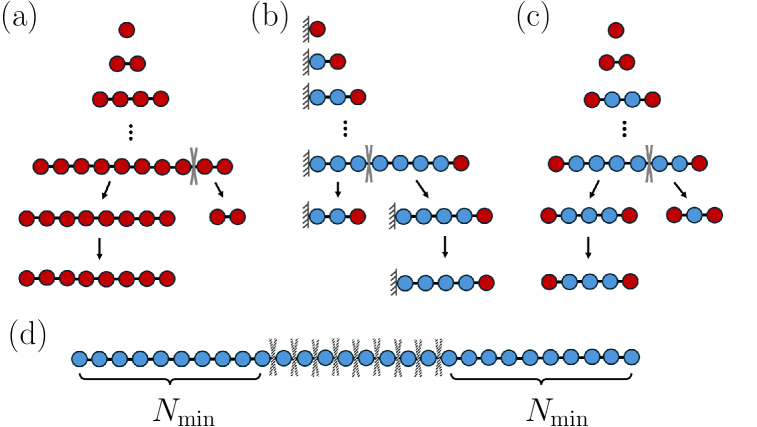
Figure 2: Growth and fracture of cell groups under different assumptions. (a) All cells can divide. After a rupture occurs, one daughter chain is selected at random. (b) Only the cell at one end of the chain can divide. (c) Only the cells at the two ends can divide. (d) Potential rupture points when a minimum cluster size $N_{\textrm{min}}$ is enforced. Rupture can only occur when the chain length $n\geqslant 2N_{\textrm{min}}$. Red cells have a non-zero division rate $k_{d}$, while blue cells have a division rate of zero; gray crosses indicate actual or potential rupture points.

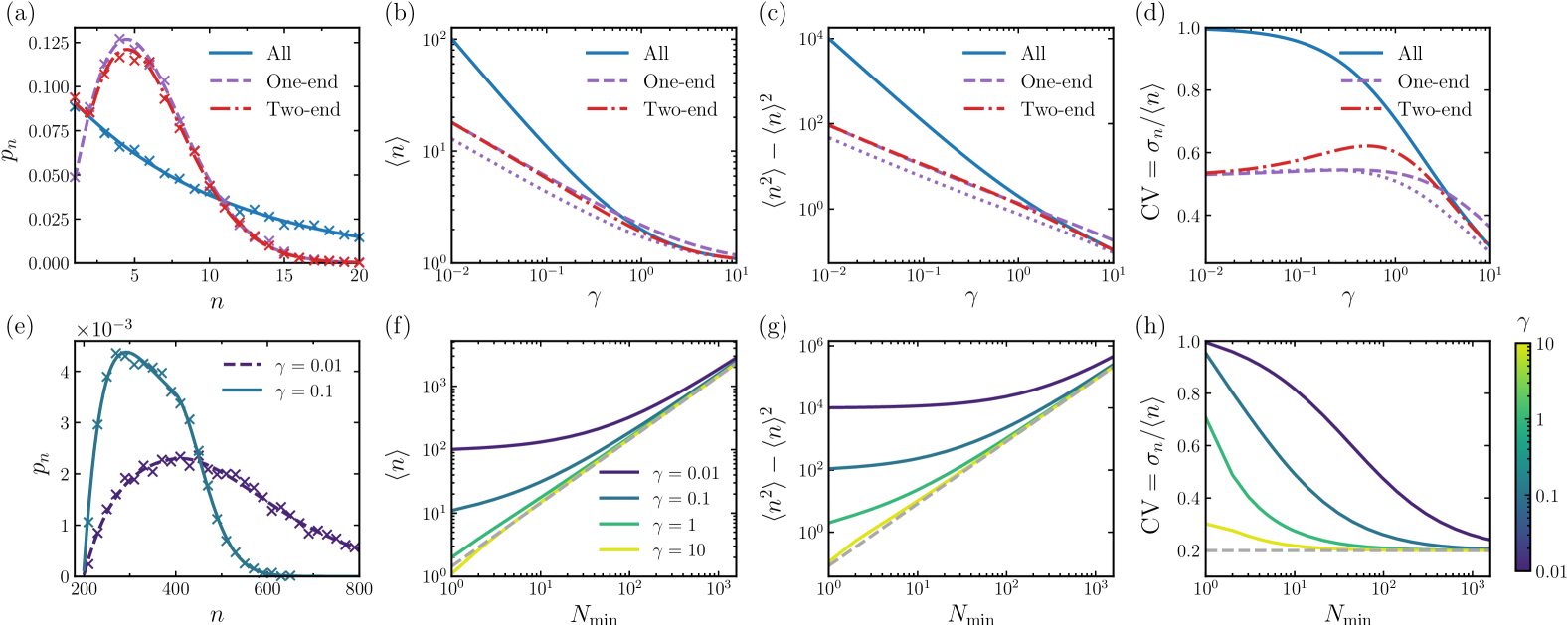
Figure 3: (a) Steady-state distribution of chain length $p_{n}$ for the three growth modes, with $\gamma=0.1$ for the all-cell growth and two-end growth models, and $\gamma$ replaced by $\gamma^{\prime}=\gamma/2=0.05$ for the one-end growth model (doubled division rate). Crosses represent simulation results, while lines correspond to theoretical predictions. Panels (b)–(d) display the mean $\langle n\rangle$, variance $\langle n^{2}\rangle-\langle n\rangle^{2}$, and coefficient of variation $\mathrm{CV}=\sigma_{n}/\langle n\rangle$, where $\sigma_{n}=\sqrt{\langle n^{2}\rangle-\langle n\rangle^{2}}$. Purple dashed lines are the one-end result after doubling the division rate [$\gamma\to\gamma^{\prime}=\gamma/2$ in Eq. (8)], while the purple dotted lines show Eq. (8). (e) Steady-state distribution $p_{n}$ when minimum cluster size $N_{\min}=200$. Crosses are simulation results, lines are theoretical predictions by the matrix method [11]. Panels (f)–(h) show how mean, variance, and CV vary with $N_{\mathrm{min}}$ in the all-cell growth model. Gray dashed lines show predictions assuming log-uniform distributions [Eq. (10)].

So far, we have assumed that all cells in the chain can divide. However, cell division may be regulated by mechanical and spatial constraints. Cells with fewer neighbors or experiencing lower compression are more likely to divide—“contact inhibition of proliferation” [18]. As an extreme limit of contact inhibition, we develop alternate models where only cells at the chain ends divide. First, consider the case where only one end of the chain grows—e.g., if the other end is constrained by a barrier. In contrast to the all-cell growth model, where the total growth rate scales as $k_{d}n$ (proportional to chain length), in one-end growth, the total growth rate is fixed at $k_{d}$ [Fig. 2(b)]. Here, the master equation becomes

$$\frac{\mathrm{d}p_{n}}{\mathrm{d}t}=\sum_{m>n}k_{b}p_{m}-p_{n}\sum_{i+j=n}k_{b}+k_{d}p_{n-1}-k_{d}p_{n}.$$ (7)

We find that the steady-state solution is

$$p_{n}={n\gamma^{1-n}}\Big{/}{\left(\dfrac{1+\gamma}{\gamma}\right)_{n}},~~~\textrm{(one-end growth)}$$ (8)

where $(x)_{n}=x(x+1)(x+2)\cdots(x+n-1)$ is the Pochhammer symbol [11]. When $\gamma\ll 1$, $p_{n}$ can be approximated by a Rayleigh distribution $n\gamma\mathrm{e}^{-\gamma n^{2}/2}$ with mode $1/\sqrt{\gamma}$.

If the chain can grow from both ends, i.e., only the two cells at the two ends can divide, the total growth rate is $2k_{d}$, except when $n=1$ (the chain has only one particle) where the total growth rate is $k_{d}$ [Fig. 2(c)]. For this case, the steady-state solution is [11]

$$p_{n}=\begin{cases}\gamma/(1+\gamma)^{n},&n=1,2,\\ \dfrac{2+\gamma}{2(1+\gamma)}\dfrac{n(\gamma/2)^{1-n}}{\bm{(}(2+\gamma)/\gamma\bm{)}_{n}},&n>2.\end{cases}~~~\textrm{(two-end)}$$ (9)

In the limit of rare breaking $\gamma\ll 1$ when clusters almost always have two ends, $p_{n}$ converges to Eq. (8) with a doubled division rate.

Figure 3(a) shows our theoretical predictions $p_{n}$ for the three growth models, validated by Monte Carlo simulations of chain evolution [11]. If all cells can divide, the cluster size distribution is extremely broad with a peak at $n=1$; if only end cells divide, we have a better-defined peak at $n\approx 1/\sqrt{\gamma}$.

Larger growth rates relative to break rates lead to larger clusters, but does this also result in greater variability of cluster size? With the distributions $p_{n}$, we can compute the means and variances of $n$ [Figs. 3(b) and 3(c)]. In the limit $\gamma\to 0$, fragmentation is rare, leading to both increased growth and increased variability in all models, while in the limit $\gamma\gg 1$, fragmentation dominates, and clusters become single-celled. To quantify the relative variability, we plot the ratio of the standard deviation of cluster size to the mean (coefficient of variation $\mathrm{CV}$) in Fig. 3(d). We see a key difference between the end-growth models and the all-growth model when $\gamma\ll 1$ and cluster sizes are large—$\mathrm{CV}$ approaches $1$ for the all-growth model, while it approaches $\sqrt{(4-\pi)/\pi}\approx 0.523$ for end-growth. The CV for end-growth is roughly half that for all-growth, indicating better size control. If the interior cells can still divide, but at a lower rate, the CV is intermediate between end- and all-growth [11].

We have so far assumed all rupture rates to be identical, but secreted factors [19] or stress [20] may vary across the cluster. As a simple model of these effects, we assume that only the junctions sufficiently far from the cluster edge break. This is equivalent to introducing a minimum cluster size $N_{\textrm{min}}$ [Fig. 2(d)]. Once we include the constraint that all clusters are larger than $N_{\textrm{min}}$, we cannot solve the master equation analytically. However, in the steady state, we can write it simply as a matrix equation $\bm{K}\mathbf{p}=\mathbf{0}$ which can be easily solved numerically to find $\mathbf{p}$ [11]. This method leads to good agreement with stochastic simulations [Fig. 3(e)].

In the absence of a minimum cluster size, large cluster sizes always come with an unavoidable variability [Figs. 3(b)–3(d)], while large rupture rates $\gamma\gg 1$ lead to sizes being precise but $\langle n\rangle\to 1$. Given a minimum cluster size, it’s possible to have precise size control and finite clusters [Figs. 3(e)–3(h)]. In the limit $\gamma\gg 1$, cell clusters grow from size $N_{\textrm{min}}$ to $2N_{\textrm{min}}$, then fragment in half. This is very similar to the dynamics of a single cell’s growth, akin to a sizer model [21, 22], and leads to distributions $p_{n}$ [Fig. 3(e)] like those of single cell size distributions [21, 23, 22, 24]. During each growth cycle $t\in[0,t_{c}]$, we have $\langle n\rangle=N_{\textrm{min}}\mathrm{e}^{k_{d}t}$ if all cells can divide, where $t_{c}=\ln 2/k_{d}$ is the time required to double the chain’s length. Over a long trajectory, any moment within the chain’s lifecycle is equally likely to be sampled [21]. If $t$ is uniformly distributed in one cycle $[0,t_{c}]$, then $p_{n}$ should obey a log-uniform distribution, as shown in Fig. S1(e) in the Supplemental Material [11]:

$$p_{n}=\frac{1}{n\ln 2},~~~n\in[N_{\textrm{min}},2N_{\textrm{min}}],$$ (10)

where the mean is $\langle n\rangle=N_{\textrm{min}}/\ln 2$ and the variance is $\langle n^{2}\rangle-\langle n\rangle^{2}=(3\ln 2-2)\langle n\rangle^{2}/2$, i.e., the coefficient of variation $\mathrm{CV}$ is independent of $N_{\textrm{min}}$, as shown in Figs. 3(f)–3(h). Similarly, if only edge cells can divide, the chain length increases linearly with time. $p_{n}$ is then uniformly distributed in $[N_{\textrm{min}},2N_{\textrm{min}}]$, leading to a mean of $3N_{\textrm{min}}/2$ and a variance of $N^{2}_{\textrm{min}}/12$. When $\gamma\gg 1$, we see mean cluster size scales as $N_{\textrm{min}}$ and the variance scales as $N^{2}_{\textrm{min}}$, but the $\mathrm{CV}$ goes to a nonzero constant as $\gamma\gg 1$, and is smaller than for clusters with no minimum size. If we weaken the strict assumption of a minimum cluster size by assuming a basal break rate $k_{b}^{0}$ for all junctions, even small $k_{b}^{0}$ creates a relevant population of small clusters [11].

Combining mechanics and statistics.—According to our theory, the break rate $k_{b}$ depends on four key parameters related to cell motility and mechanical properties of the cluster—$\tau$, $\mu k$, $D$, and $\delta\ell_{b}$. While these parameters have not yet been measured simultaneously for a single cell type, we can provide reasonable estimates. Experiments measuring velocity correlations of HaCaT cells [25] give a persistence time $\tau$ of roughly $0.5$ hour and $D$ of around $\sim 100\,\mathrm{\mu m^{2}/h}$, leading to an active velocity $v_{n}$ on the order of $\sqrt{D/\tau}\approx 15\,\mathrm{\mu m/h}$. The mobility $\mu$ and spring constant $k$ together create a relaxation timescale $1/\mu k$, estimated to be approximately $15\,\mathrm{min}$ based on measurements for MDCK cells [8] (details in SM [11]). According to Eq. (4), the break rate $k_{b}$ is highly sensitive to the critical break length $\delta\ell_{b}$. As a rough guess, $\delta\ell_{b}=5\,\mathrm{\mu m}$ yields a mean escape time $\tau_{\mathrm{esc}}\approx 17.6\,\mathrm{h}$, or a break rate of approximately $0.057\,\mathrm{h^{-1}}$. This is the right order of magnitude for experiments in germline cyst fracture [3] and cancer cell dissociation [5, 6]. We use these values as our default parameters (Table S1 in [11]).

Our results suggest that clusters of cells may regulate their size not only by changing division rate but also by changing cell motility or persistence or cell-cell adhesion. Recent experiments found that germline cells have motility that decreases as cysts develop, decreasing fracture over time and controlling cyst size [3]. How much does a change in cell properties change cluster size? The break rate and division rate of germline cysts are approximately $0.02\,\mathrm{h^{-1}}$ and $0.04\,\mathrm{h^{-1}}$ [3], i.e., the ratio $\gamma\approx 0.5$, corresponding to a mean cluster size $\langle n\rangle\approx 3$ in the all-cell growth model. (We note this is not the value found by Ref. [3]—their germline cysts do not reach the steady state. If we simulate for only $5$ division times, we get similar results to their experiment and model [11].) For germline cysts, we set $\delta\ell_{b}=6.5\,\mathrm{\mu m}$ to match $k_{b}$ to experiment. Cell motility and cell-cell adhesion change $k_{b}$ and thus change $\gamma$, changing cluster size distributions. For instance, if cells double their adhesiveness by increasing $k$, $\gamma$ decreases to approximately $0.0067$, leading to a larger cluster size $\langle n\rangle\approx 150$ with significantly higher variability $\sigma_{n}\approx 150$. At long developmental times, the break rate of germline cysts drops to under $1/190\,\mathrm{h^{-1}}$, which Ref. [3] attributes to changes in cell motility. We find this drop does not require a dramatic change in cell speed. To decrease the break rate to this level, $D$ must decrease by more than a factor of $1.5$, i.e., the typical speed of cells needs to decrease by more than a factor of $1.2$.

Discussion.—Our work provides a route to understand quantitatively how the size of groups of cells ranging from cancer to organs to organisms can emerge from balancing growth and random cell motility. Our model shows that differences in where cell division and rupture occur can lead to different characteristic distributions of cluster sizes, and that biologically relevant regulation of cluster size can occur from relatively small changes in cell motility. From a physics standpoint, our results show that even in a very simple one-dimensional active material, the collective rupture of a link is nontrivial and can’t be understood from the properties of a single pair of cells—unlike in an equilibrium version of our model. This qualitative difference with the simple active trap model [10] suggests that rupture rates may be sensitive to other collective features, e.g., differing between branched and linear chains of cells, or reflecting the degree of cell-cell correlation of velocities.

We have generally chosen analytic tractability over biological detail in our approach to capture the key elements of this problem. There are many possible generalizations. These include polymer networks within the cell [26], cell-matrix interactions [27, 28], cell shape [6, 29] and its coupling to division [30, 18], or mechanosensitive feedback [31], as well as cell-cell interactions like contact inhibition of locomotion [32, 33, 34] and collective alignment of cell polarity [35, 8]. Determining to what extent these features only change the relevant energy barrier, rescaling $k$, or qualitatively change our picture is an important open question.