Two-Round Distributed Principal Component Analysis: Closing the Statistical Efficiency Gap

Abstract

We enhance Fan et al.’s (2019) one-round distributed principal component analysis algorithm by adding a second fixed-point iteration round. Random matrix theory reveals the one-round estimator exhibits higher asymptotic error than the pooling estimator under moderate local signal-to-noise ratios. Remarkably, our second iteration round eliminates this efficiency gap. It follows from a careful analysis of the first-order perturbation of eigenspaces. Empirical experiments on synthetic and benchmark datasets consistently demonstrate the two-round method’s statistical advantage over the one-round approach.

Keywords: Distributed learning; Random matrix theory; Fixed-point iteration.

1 Introduction

Principal component analysis (PCA) remains the cornerstone technique for dimensionality reduction (Pearson,, 1901), with applications spanning regression, functional analysis, and factor modeling (Jolliffe et al.,, 2003; Fan et al.,, 2013; Chen and Fan,, 2023; He et al.,, 2022). The primary objective of principal component analysis is to lower the dimensionality of a dataset while preserving the maximal amount of original variance. This is achieved by computing the eigenvectors and eigenvalues of the sample covariance matrix, where the eigenvectors correspond to the principal directions of variance, and the eigenvalues quantify the extent of variability along these directions.

In this era of information, large datasets are often scattered across distant machines. The attempt to fuse or aggregate these datasets is extremely difficult. Over the past two decades, significant progress has been made in the development of distributed PCA, contributing to the broader efforts to create accurate and efficient distributed statistical methods. In general, there are two data partition regimes for distributed PCA. For horizontal partition, each local machine contains all the features of a subset of subjects (Qu et al.,, 2002). Meanwhile, for vertical partition, each machine has a subset of features of the same group of subjects. It has roots in sensor networks and signal processing (Kargupta et al.,, 2001; Schizas and Aduroja,, 2015).

In this work, we focus on horizontal partition. However, the algorithms in this work could also be applied to the vertical partition settings, thanks to the symmetry of columns and rows in rank $r$ approximation (Qu et al.,, 2002; Fan et al.,, 2019).

For horizontal partition, Fan et al., (2019) proposed a novel one-round distributed principal component analysis algorithm. In the one-round algorithm, the local machines only send the leading eigenvectors to the central machine, on which the local subspace information is integrated. Their analysis demonstrated matching statistical error rates with pooling PCA, i.e., PCA over the full sample, but only under high local signal-to-noise ratio conditions.

However, when the local datasets have moderate signal-to-noise ratios (due to small sample sizes or weak signals), existing one-round subspace integration theory no longer holds (Fan et al.,, 2019; Li et al.,, 2024). Random matrix theory provides analytical tools for these scenarios (Marchenko and Pastur,, 1967; Bai and Silverstein,, 2010; Couillet and Liao,, 2022). Our work examines method performance under moderate local signal-to-noise ratio conditions.

1.1 Problem formulation

We discuss the problem under the classical Gaussian spiked covariance model (Paul,, 2007). We follow Fan et al., (2019) and assume homogeneous sub-sample sizes. Namely, we have $K$ machines, each containing $n$ observations, denoted as $\{x_{i}^{k}\}^{k\in[K]}_{i\in[n]}$. We assume that $x_{i}^{k}\in{\mathbb{R}}^{p}$ are i.i.d. Gaussian random vectors with zero mean and a homogeneous population covariance matrix $\Sigma=\sum_{i=1}^{r}l_{i}u_{i}u_{i}^{\top}+I_{p}$, whose leading $r$ eigenvectors form a $p\times r$ column orthogonal matrix $U:=(u_{1},\dots,u_{r})$. Principal component analysis aims to retrieve $U$ from noisy observations.

In the large local signal-to-noise ratio regime, i.e., $n\gg p$ or $l_{i}\gg 1$ for $i\in[r]$, it is shown in Fan et al., (2019) that the one-round distributed PCA estimator has the same convergence rate as the pooling PCA estimator, and extensive empirical experiments support this claim. To the best of our knowledge, no theoretical analysis has been made for the one-round subspace integration method with moderate local signal-to-noise ratios (Fan et al.,, 2019; Li et al.,, 2024). However, it is believed that the moderate local signal-to-noise ratios could be found in many real-world problems, as datasets are often scattered across a large number of local machines such as smartphones and personal computers, each containing a relatively small sample size.

To close this theoretical gap, in this work, we assume that $p/n\rightarrow c$ as $n$, $p\rightarrow\infty$. Meanwhile, $r$ and $l_{1}>l_{2}>\dots>l_{r}$ will be treated as constants, so that the local datasets have moderate signal-to-noise ratios. Due to the well-known phase transition phenomenon in the random matrix theory (Paul,, 2007; Couillet and Liao,, 2022), the $r$-th eigenvector information is lost for the local machines unless the spike $l_{r}$ exceeds the local phase transition threshold, namely $l_{r}>\sqrt{c}$. For the one-round distributed PCA to work, we shall assume that $l_{r}>\sqrt{c}$ throughout this work, as it makes little sense to study one-round distributed PCA under this signal threshold. Finally, $K$ also diverges, but we do not restrict its order of divergence. It implies that $N:=Kn\gg p$, so that the pooling PCA estimator is still consistent, and we can then compare the asymptotic efficiency of different methods.

It is possible to generalize the model setting above. For instance, all algorithms in this work are capable of handling heterogeneous local sample sizes and $n$ could be generalized to $n_{k}$. Also, we can relax the Gaussian assumption to, e.g., finite fourth moments, together with conditions like symmetric innovation as in Fan et al., (2019), keeping almost all theoretical arguments unchanged. However, the main purpose of this work is to show that the one-round distributed PCA algorithm is not asymptotically efficient. Meanwhile, we present a two-round algorithm that achieves asymptotic efficiency. The setting above suffices for such a purpose and saves us from heavy notations, providing a clearer picture. Hence, we shall discuss under the model setting given in this section.

1.2 Contributions

In this article, we study the statistical convergence of one-round distributed PCA, whose communication cost is of order $O(Kpr)$, under moderate local signal-to-noise ratios. It is shown that the one-round distributed PCA estimator has a larger asymptotic statistical error than the pooling PCA estimator, whose communication cost is of order $O(Kpn)$, unless the local signal-to-noise ratio diverges.

We propose to conduct another communication round that resembles the fixed-point iteration (also known as the power method) when calculating eigenvectors in numerical algebra (Ford,, 2014), resulting in the total communication cost of merely $O(3Kpr)$. It is then shown both theoretically and empirically that this additional round suffices for achieving asymptotic efficiency. The theoretical claim comes from a careful analysis of the first-order perturbation of eigenspaces.

Finally, the proposed two-round distributed PCA algorithm is applied on synthetic datasets and the benchmark tabular datasets from Grinsztajn et al., (2022). Besides validating our theoretical arguments, we show that the two-round algorithm has a persistent statistical advantage over the one-round algorithm in empirical experiments.

2 One-round Distributed PCA

In this section, we first introduce the notion of asymptotic efficiency used in this paper. Then, we study the statistical performance of the one-round distributed PCA estimator proposed by Fan et al., (2019) under the settings in Section 1.1. It is shown that the one-round distributed PCA is not asymptotically efficient in the moderate local signal-to-noise ratio regime.

If we transfer all data to the central machine, we acquire a pooled dataset of sample size $N=K\times n$, with the communication cost of $O(Kpn)$. We have the following pooled sample covariance matrix $\widehat{\Sigma}^{\mathcal{P}}:=\sum_{k=1}^{K}\sum_{i=1}^{n}x_{i}^{k}(x_{i}^{k})^{\top}/N$. Its leading $r$ eigenvectors form a $p\times r$ column orthogonal matrix $\widehat{U}^{\mathcal{P}}:=(\widehat{u}_{1}^{\mathcal{P}},\dots,\widehat{u}_{r}^{\mathcal{P}})$. We call $\widehat{U}^{\mathcal{P}}$ the pooling PCA estimator. It stands as the goal of the distributed PCA algorithms.

We now introduce the notion of asymptotic efficiency in the context of distributed PCA. In particular, we say any distributed PCA estimator $\widehat{U}$ is asymptotically efficient if and only if it is as good as the pooling PCA estimator in an asymptotic subspace variance manner.

Definition 2.1 (Asymptotic efficiency).

For any distributed PCA estimator $\widehat{U}$ and the pooling PCA estimator $\widehat{U}^{\mathcal{P}}$, we define the asymptotic subspace variance ratio as

$$\mathcal{V}\left(\widehat{U}\right):=\frac{{\mathbb{E}}\left(\left\|\widehat{U}\widehat{U}^{\top}-UU^{\top}\right\|^{2}_{F}\right)}{{\mathbb{E}}\left(\left\|\widehat{U}^{\mathcal{P}}(\widehat{U}^{\mathcal{P}})^{\top}-UU^{\top}\right\|^{2}_{F}\right)}.$$

We say the distributed PCA estimator $\widehat{U}$ is asymptotically efficient if and only if

$$\lim\limits_{k\rightarrow\infty}\lim\limits_{n,p\rightarrow\infty}\mathcal{V}\left(\widehat{U}\right)=1.$$

According to Fan et al., (2019), we do not need to transfer all data to the central machine, but can respectively calculate local sample covariance matrices $\widetilde{\Sigma}_{k}:=\sum_{i=1}^{n}x_{i}^{k}(x_{i}^{k})^{\top}/n$, for $k\in[K]$ whose leading $r$ eigenvectors form a $p\times r$ column orthogonal matrix $\widetilde{U}_{k}:=(\widetilde{u}^{k}_{1},\dots,\widetilde{u}^{k}_{r})$. We only send $\widetilde{U}_{k}$ to the central machine, resulting in the total communication cost of $O(Kpr)$. Then, the central machine calculates the leading $r$ eigenvectors of

$$\widehat{\Sigma}^{(1)}:=\frac{1}{K}\sum_{k=1}^{K}\widetilde{U}_{k}\widetilde{U}^{\top}_{k},$$

denoted as $\widehat{U}^{(1)}:=(\widehat{u}_{1}^{(1)},\dots,\widehat{u}_{r}^{(1)})$, which is called the one-round distributed estimator in this article. Here the superscript $(1)$ means one round of communication.

Theorem 1 (One-round distributed PCA).

Under the settings in Section 1.1, we have

$$\lim\limits_{k\rightarrow\infty}\lim\limits_{n,p\rightarrow\infty}\mathcal{V}\left(\widehat{U}^{(1)}\right)=\frac{\sum_{i=1}^{r}(pl_{i}^{-1}+pl_{i}^{-2})/(n-pl_{i}^{-2})}{\sum_{i=1}^{r}(pl_{i}^{-1}+pl_{i}^{-2})/n}>1.$$

From Theorem 1, we notice that the asymptotic subspace variance ratio of the one-round distributed PCA estimator depends heavily on the local signal-to-noise ratio, which is characterized by $n$, the local sample size, $p$, the data dimension, and $l_{i}$, the signal strength. For notational convenience, we let the local signal-to-noise ratio correspond to the weakest signal spike, namely define it as $nl_{r}^{2}/p$. If $n\gg pl_{r}^{-2}$, i.e., the local signal-to-noise ratio diverges, then we have $\lim_{k\rightarrow\infty}\lim_{n,p\rightarrow\infty}\mathcal{V}(\widehat{U}^{(1)})\rightarrow 1$ and the one-round PCA estimator tends to be asymptotically efficient. Meanwhile, note that we have assumed that $n>pl_{r}^{-2}$ in the Introduction. Due to the phase transition phenomenon in the random matrix theory, if $n\leq pl_{r}^{-2}$, i.e., $l_{r}\leq\sqrt{p/n}$, the $r$-th eigenvector information will be lost. As $n\rightarrow pl_{r}^{-2}$ from above, we shall have $\lim_{k\rightarrow\infty}\lim_{n,p\rightarrow\infty}\mathcal{V}(\widehat{U}^{(1)})\rightarrow\infty$ and the one-round distributed estimator is questionable. In conclusion, the one-round distributed PCA estimator has a larger asymptotic statistical error than the pooling PCA estimator, unless the local signal-to-noise ratio $nl_{r}^{2}/p\rightarrow\infty$. The arguments above are validated by numerical experiments, as will be shown later.

3 Two-round Distributed PCA

In the previous section, we show that the one-round distributed PCA has a larger statistical error than the pooling estimation, under moderate local signal-to-noise ratios. However, the communication cost of pooling PCA is of order $O(Kpn)$, much larger than $O(Kpr)$, the communication cost of the one-round distributed PCA. With this problem in mind, we present a two-round distributed PCA algorithm in this section, which includes an additional step of fixed-point iteration. The proposed two-round estimator achieves the asymptotic efficiency of pooling PCA with merely the communication cost of $O(3Kpr)$.

In the first round, we use the one-round distributed PCA algorithm to acquire $\widehat{U}^{(1)}$, with the communication cost $O(Kpr)$. In the second round, the central machine sends $\widehat{U}^{(1)}$ back to the local machines. This step also costs $O(Kpr)$ of communication. Then, the local machines send $\widetilde{G}_{k}:=\widetilde{\Sigma}_{k}\widehat{U}^{(1)}\in{\mathbb{R}}^{p\times r}$ to the central machine. Hence, the communication cost adds up to $O(3Kpr)$. Finally, the central machine orthogonalizes $\widehat{G}=\sum_{k=1}^{K}\widetilde{G}_{k}/K\in{\mathbb{R}}^{p\times r}$ to acquire $\widehat{U}^{(2)}$. We use $\widehat{U}^{(2)}$ as the two-round distributed PCA estimator. The procedures above are organized in the following Algorithm 1.

Algorithm 1 Two-round distributed principal component analysis.

0:   $\widetilde{\Sigma}_{k}$ for $k\in[K]$; cut-off dimension $r$;

0:   

1: the first round: the local machines send the local leading eigenvectors $\widetilde{U}_{k}$ to the central machine; the central machine acquire the one-round distributed PCA estimator $\widehat{U}^{(1)}$ by calculating the leading $r$ eigenvectors of $\widehat{\Sigma}^{(1)}=\sum_{k=1}^{K}\widetilde{U}_{k}\widetilde{U}^{\top}_{k}/K$;

2: the second round: the central machine sends $\widehat{U}^{(1)}$ back to the local machines; the local machines send $\widetilde{G}_{k}=\widetilde{\Sigma}_{k}\widehat{U}^{(1)}$ to the central machine; the central machine obtain $\widehat{U}^{(2)}$ by orthogonalizing $\widehat{G}=\sum_{k=1}^{K}\widetilde{G}_{k}/K$.

3: return  two-round distributed PCA estimator $\widehat{U}^{(2)}$.

Before we rigorously discuss the theoretical properties of the two-round estimator $\widehat{U}^{(2)}$, some intuitions are stated as follows. First, note that the central machine eventually gets

$$\widehat{G}=\sum_{k=1}^{K}\widetilde{G}_{k}/K=\left(\sum_{k=1}^{K}\widetilde{\Sigma}_{k}/K\right)\widehat{U}^{(1)}=\widehat{\Sigma}^{\mathcal{P}}\widehat{U}^{(1)}.$$ (1)

Namely, the central machine almost acquires the pooled sample covariance matrix $\widehat{\Sigma}^{\mathcal{P}}$ painlessly, by merely an additional $O(2Kpr)$ communication cost. Second, (1) resembles the fixed-point iteration (also known as the power method) when calculating the eigenvectors of $\widehat{\Sigma}^{\mathcal{P}}$ in numerical algebra (Ford,, 2014). It is foreseeable that if such iteration proceeds, $\widehat{U}^{(t)}$ shall tend to the leading eigenvalues of $\widehat{\Sigma}^{\mathcal{P}}$ as $t\rightarrow\infty$, in a linear convergence rate. Fortunately, thanks to the tangent nature of eigenspace perturbations, we manage to show that we do not need a large number of iteration steps. In fact, we witness a “super convergence”, i.e., one more round of communication suffices for the resulting estimator to be asymptotically efficient.

Theorem 2 (Two-round distributed PCA).

Under the settings in Section 1.1, we have

$$\lim\limits_{k\rightarrow\infty}\lim\limits_{n,p\rightarrow\infty}\mathcal{V}\left(\widehat{U}^{(2)}\right)=1.$$

Theorem 2 follows from a careful first-order eigenspace perturbation analysis. Let $\Delta^{(1)}:=\widehat{U}^{(1)}(\widehat{U}^{(1)})^{\top}-\widehat{U}^{\mathcal{P}}(\widehat{U}^{\mathcal{P}})^{\top}$, and define $\widehat{\mathcal{U}}^{\mathcal{P}}:=(\widehat{U}^{\mathcal{P}},\widehat{U}^{\mathcal{P}}_{\perp})$, the central machine eventually calculates the leading $r$ eigenvectors of

$$\widehat{\Sigma}^{(2)} :=\widehat{\Sigma}^{\mathcal{P}}\widehat{U}^{(1)}(\widehat{U}^{(1)})^{\top}\widehat{\Sigma}^{\mathcal{P}}=\widehat{\Sigma}^{\mathcal{P}}\widehat{U}^{\mathcal{P}}(\widehat{U}^{\mathcal{P}})^{\top}\widehat{\Sigma}^{\mathcal{P}}+\widehat{\Sigma}^{\mathcal{P}}\Delta^{(1)}\widehat{\Sigma}^{\mathcal{P}}$$ (2)

$$=\underbrace{\widehat{\Sigma}^{\mathcal{P}}\widehat{U}^{\mathcal{P}}(\widehat{U}^{\mathcal{P}})^{\top}\widehat{\Sigma}^{\mathcal{P}}}_{\text{signal}}+\underbrace{\widehat{\Sigma}^{\mathcal{P}}\widehat{\mathcal{U}}^{\mathcal{P}}\widehat{L}^{(1)}(\widehat{\mathcal{U}}^{\mathcal{P}})^{\top}\widehat{\Sigma}^{\mathcal{P}}}_{\text{tangent first-order}}+\underbrace{\widehat{\Sigma}^{\mathcal{P}}\widehat{R}^{(1)}\widehat{\Sigma}^{\mathcal{P}}}_{\text{higher-order}},$$

where the decomposition $\Delta^{(1)}=\widehat{\mathcal{U}}^{\mathcal{P}}\widehat{L}^{(1)}(\widehat{\mathcal{U}}^{\mathcal{P}})^{\top}+\widehat{R}^{(1)}$ comes from Lemma 2 of Fan et al., (2019), the higher-order Davis-Kahan theorem.

We take a closer look at each term in (2) respectively. First, the signal $\widehat{\Sigma}^{\mathcal{P}}\widehat{U}^{\mathcal{P}}(\widehat{U}^{\mathcal{P}})^{\top}\widehat{\Sigma}^{\mathcal{P}}$ is of rank $r$. Its non-trivial eigenvectors are exactly $\widehat{U}^{\mathcal{P}}$. Its non-trivial eigenvalues are $(\widehat{\lambda}_{i}^{\mathcal{P}})^{2}$ for $i\in[r]$. Second, $\widehat{L}^{(1)}$ is almost as large as $\Delta^{(1)}$, so the tangent term $\widehat{\Sigma}^{\mathcal{P}}\widehat{\mathcal{U}}^{\mathcal{P}}\widehat{L}^{(1)}(\widehat{\mathcal{U}}^{\mathcal{P}})^{\top}\widehat{\Sigma}^{\mathcal{P}}$ is relatively large in size. Fortunately, we do not need to treat it as “noise” in the matrix perturbation theory, as this term is tangent to the signal term and only contributes to the eigenvectors with respect to smaller eigenvalues. Finally, the real “noise” is indeed the higher-order term $\widehat{\Sigma}^{\mathcal{P}}\widehat{R}^{(1)}\widehat{\Sigma}^{\mathcal{P}}$, which tends to $0$ rapidly and is negligible. One interesting aspect of (2) is that the observed matrix $\widehat{\Sigma}^{(2)}$ is in fact of rank $r$. To acquire proof, we deliberately decompose $\widehat{\Sigma}^{(2)}$ into a high rank “signal plus tangent” part with desired leading eigenvectors, and a higher-order “noise”.

To end this section, we point out that another by-product of two-round distributed PCA is the spiked eigenvalue estimation. In one-round distributed PCA, the local eigenvalue information is discarded. In the second round, fortunately, the central machine is able to receive the signal eigenvalue information from the local machines. For $i\in[r]$, we use the $i$-th largest singular value of $\widehat{G}$, denoted as $\widehat{\lambda}^{(2)}_{i}$, to be the estimator of $\lambda_{i}:=l_{i}+1$.

Corollary 1 (Spiked eigenvalue estimation).

Under the settings in Section 1.1, for $i\in[r]$, let $\widehat{\lambda}^{\mathcal{P}}_{i}$ be the $i$-th eigenvalue of the pooled covariance matrix $\widehat{\Sigma}^{\mathcal{P}}$. We have $\widehat{\lambda}_{i}^{(2)}-\widehat{\lambda}^{\mathcal{P}}_{i}=O_{p}(K^{-1})$.

In Corollary 1, we show that $\widehat{\lambda}^{(2)}_{i}$ is asymptotically equivalent to the pooling spiked eigenvalue estimator $\widehat{\lambda}^{\mathcal{P}}_{i}$. The latter has been extensively studied; one can refer to, e.g., Theorem 2.13 in Couillet and Liao, (2022).

4 Numerical Experiments

In this section, we conduct numerical experiments on synthetic datasets and benchmark tabular datasets, to validate our theoretical claims and also demonstrate the empirical advantage of the proposed two-round method. One can find the codes to reproduce all numerical results in this work at https://github.com/LZeY-FD/2RDPCA.

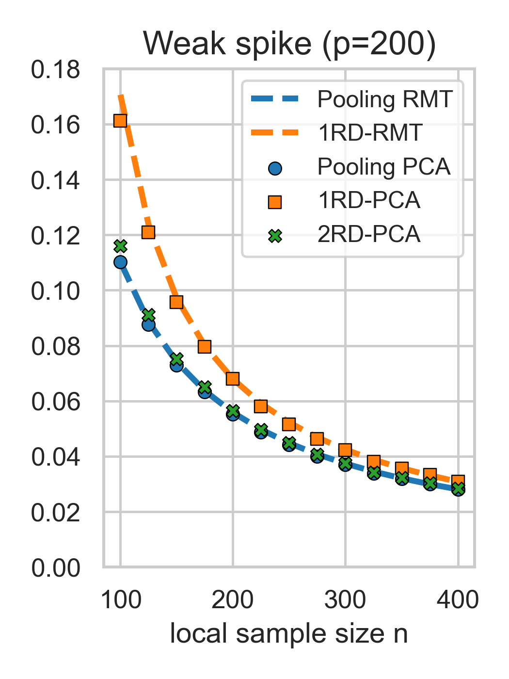
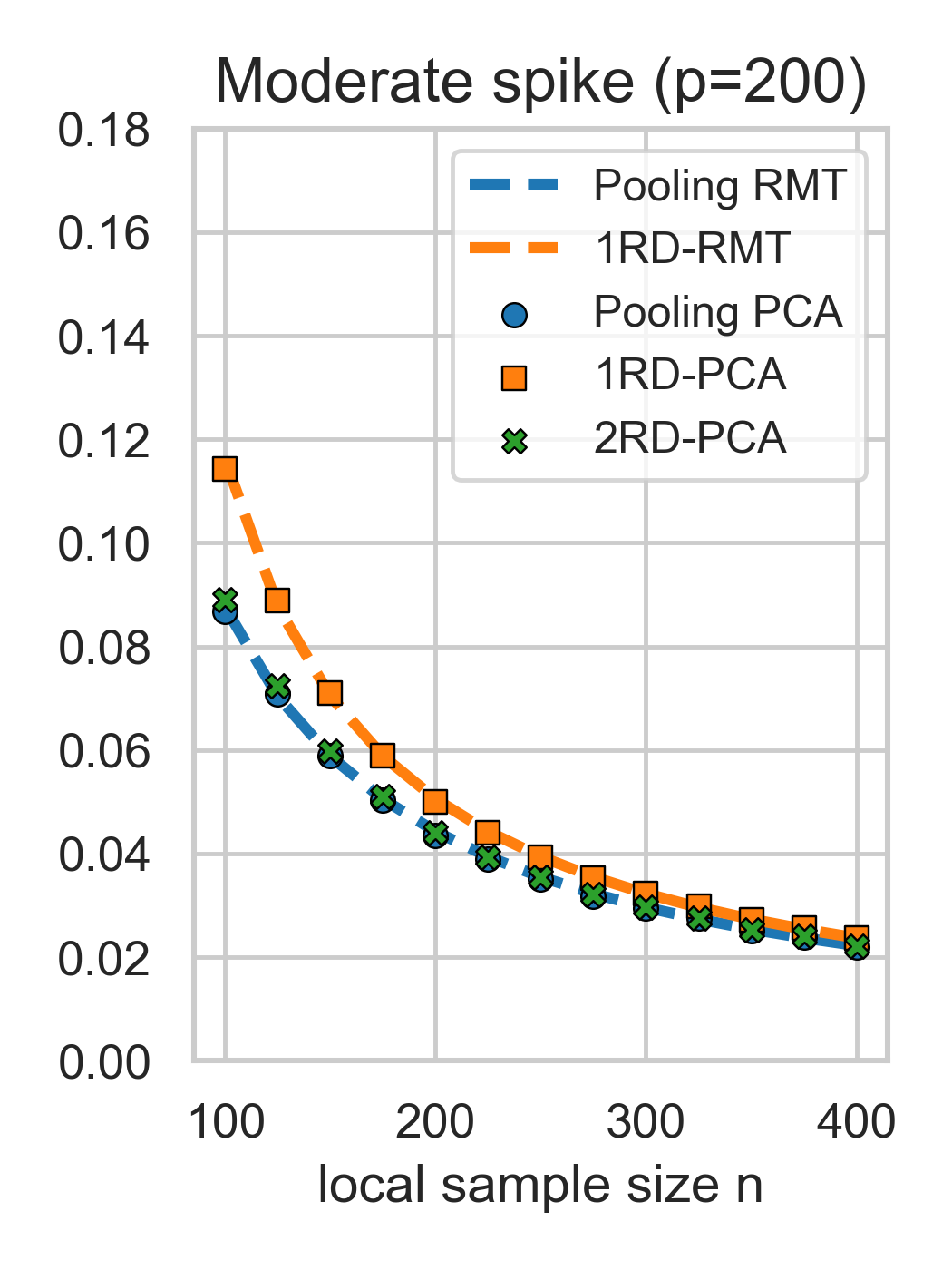
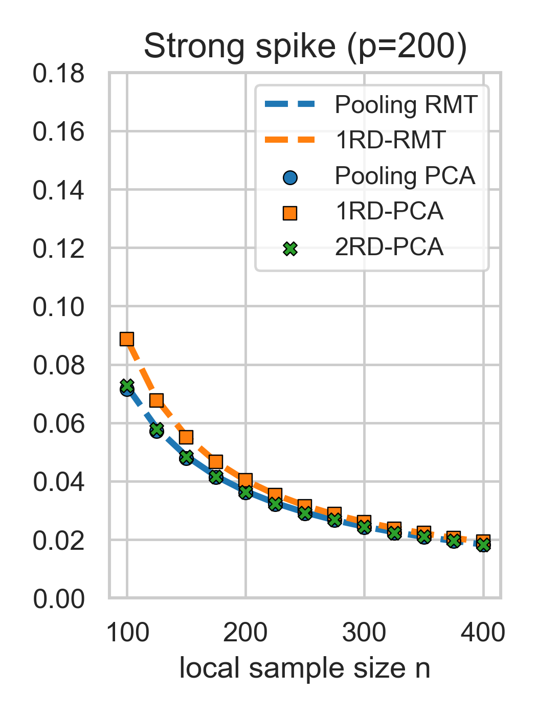
Figure 1: Mean squared subspace estimation error of different estimators on synthetic datasets. The results are based on $100$ replications as $n$ ranges from $100$ to $400$, against the theoretical rates from the random matrix theory (RMT), with respect to relatively weak spike, moderate spike and relatively strong spike.

First, we generate synthetic datasets to validate our theoretical arguments. We generate independent centered Gaussian random vectors with spike strength

$$(l_{1},l_{2},l_{3})\in\{(2.75,2.5,2.25),(3.25,3,2.75),(3.75,3.5,3.25)\},$$

corresponding to three scenarios: relatively weak spike, moderate spike, and relatively strong spike. We set $p=200$ and $K=30$, while $n$ ranges from $100$ to $400$. In Figure 1, we report the mean squared subspace estimation error, as measured by $\|\cdot-UU^{\top}\|_{F}^{2}/2$, of different estimators, based on $100$ replications.

We can see that the mean squared subspace estimation error of the pooling PCA estimator and the one-round distributed PCA estimator matches the theoretical rates derived from random matrix theory. As predicted by Theorem 1, the one-round distributed PCA estimator tends to be more efficient as the local signal-to-noise ratio increases, i.e., either $n$ or $l_{i}$ gets larger. However, the one-round distributed PCA estimator still has a larger statistical error than the pooling PCA estimator, under relatively weaker local signal-to-noise ratios. Meanwhile, the two-round distributed PCA estimator manages to achieve similar statistical performance as the pooling PCA estimator, with merely $O(3Kpr)$ cost of communication.

Figure 2: The relative performace of one-round and two-round distributed PCA estimators against the pooling PCA estimator, over 20 selected benchmark tabular datasets, based on $100$ replications.

Then, we apply the distributed PCA algorithms to the benchmark tabular datasets from Grinsztajn et al., (2022). In Grinsztajn et al., (2022), the authors compiled 45 tabular datasets from various domains, provided mostly by OpenML. The benchmark consists of four splits based on tasks and datasets used for tasks, which are respectively regression on numerical features, regression on numerical and categorical features, classification on numerical features, and classification on categorical features. Thus, we are able to experiment with the distributed PCA algorithms on numerical and categorical features of these datasets. We discard the datasets with small feature dimensions ($p<20$) or large pooled sample sizes ($N>500,000$), resulting in $20$ datasets left.

In Figure 2, we report the relative performance of one-round and two-round distributed PCA estimators against the pooling PCA estimator. The statistical performance for any estimator $\widehat{U}$ is quantified by the Average information preservation Ratio (AR), defined as $\text{AR}(\widehat{U})=(\sum_{i}\|\widehat{U}\widehat{U}^{\top}x_{i}\|_{2}^{2})/(\sum_{i}\|x_{i}\|_{2}^{2})$, where $\|\cdot\|_{2}$ is the vector $\ell_{2}$ norm and $x_{i}$ could be taken from either the training or the test set. The implementation details on the benchmark datasets are left to the supplementary material for saving space.

The two-round distributed PCA algorithm shows persistent ($100\%$) statistical advantage against the one-round distributed PCA algorithm in all $20$ datasets. In particular, for the MiniBooNE dataset, which corresponds to the yellow dots in the bottom right corners of both plots in Figure 2, the one-round distributed PCA breaks down and fails to retrieve the population principal subspace. Meanwhile, the two-round distributed PCA is still robust even though the first-round subspace estimator is no longer valid. In conclusion, the second round of communication guarantees statistical efficiency at the additional cost of merely $O(2Kpr)$. Hence, we gladly recommend the proposed two-round distributed PCA algorithm for consideration in most real-world cases.

5 Discussion

In this paper, we show that the celebrated one-round distributed PCA method is not asymptotically efficient in the moderate local signal-to-noise ratio regime. Fortunately, merely one additional communication round suffices to achieve asymptotic efficiency. We experiment on synthetic and benchmark tabular datasets, where the proposed two-round algorithm shows a persistent statistical advantage over the one-round algorithm.

For possible future work, it is interesting to dive deeper into the “super convergence” phenomenon as alluded to in Section 3, namely, the cases where the first step of iteration is sufficient for statistical efficiency. Indeed, the iterative projection technique is popular in eigenspace estimation for higher-order data (Li et al.,, 2024; Xia et al.,, 2021). It is intriguing to explore the common aspects of these problems in a unified manner.

Appendix

In the Appendix, we give the implementation details of the benchmark datasets and the proof of the theoretical results.

6 Implementation Details of the Benchmark Datasets

Each benchmark dataset is viewed as a pooled dataset. Recall that we discard the datasets with small feature dimensions ($p<20$) or large pooled sample sizes ($N>500,000$), resulting in $20$ datasets left. For each remaining dataset, we randomly take $80\%$ to be the train set, and set the remaining $20\%$ as the test set. Given constants $\kappa$ and $\rho$, we split the pooled dataset into $K=\lfloor\kappa N/p\rfloor$ local machines, so that the local sample size $n$ is on the same scale as feature dimension $p$. We apply distributed PCA algorithms with cut-off dimension $r=\min(\lfloor\rho p\rfloor,r_{\max})$ for some pre-determined $r_{\max}$. In our experiments, we choose $\kappa\in\{1,2\}$, set $\rho=0.2$ and $r_{\max}=20$. Note that the statistical performance for any estimator $\widehat{U}$ is quantified by the Average information preservation Ratio (AR), defined as

$$\text{AR}(\widehat{U})=\frac{\sum_{i}\left\|\widehat{U}\widehat{U}^{\top}x_{i}\right\|_{2}^{2}}{\sum_{i}\left\|x_{i}\right\|_{2}^{2}},$$

where $\|\cdot\|_{2}$ is the vector $\ell_{2}$ norm and $x_{i}$ could be taken from either the train or test set.

Due to limited space, we only report the case with $\kappa=2$ and $\rho=0.2$ in the main article. Here we also present the results when $\kappa=1$ and $\rho=0.2$. The conclusions are almost identical.

Figure 3: The relative performace of one-round and two-round distributed PCA estimators against the pooling PCA estimator, over 20 selected benchmark tabular datasets, based on $100$ replications, with $\kappa=1$ and $\rho=0.2$.

7 Proof of Theoretical results

In this section, we give the proof of the main results in the paper.

7.1 Proof of Theorem 1

Before diving into the theoretical details, we first give a brief outline of the proof. The first step is to understand the asymptotic behavior of the pooling PCA estimator $\widehat{U}^{\mathcal{P}}$, which is rather straightforward thanks to the existing random matrix theory (Paul,, 2007; Couillet and Liao,, 2022). We know that the following Lemma 3 holds.

Lemma 3 (Pooling PCA estimator).

Under the settings in Section 1.1 of the main article, we have

$$K{\mathbb{E}}\left(\left\|\widehat{U}^{\mathcal{P}}(\widehat{U}^{\mathcal{P}})^{\top}-UU^{\top}\right\|^{2}_{F}\right)\rightarrow 2\sum_{i=1}^{r}\frac{pl_{i}^{-1}+pl_{i}^{-2}}{n}.$$

The second step is to study the asymptotic convergence of the one-round distributed estimator. First, as also shown in Fan et al., (2019), the one-round distributed PCA is unbiased under the settings in Section 1.1 of the main article, in the sense that $\text{span}(U)$ is also the leading eigenspace of $\Sigma^{(1)}:={\mathbb{E}}(\widetilde{U}_{k}\widetilde{U}^{\top}_{k})$. Then, using the matrix concentration inequality (Tropp,, 2012, 2015), we show that $\|\sum_{k=1}^{K}\widetilde{U}_{k}\widetilde{U}^{\top}_{k}/K-{\mathbb{E}}(\widetilde{U}_{k}\widetilde{U}^{\top}_{k})\|_{\mathop{\text{\rm op}}}$ tends to $0$ as $K$, $n$, $p\rightarrow\infty$. In the following, we use the higher-order Davis-Kahan theorem from Fan et al., (2019) to carefully separate the linear matrix perturbation error from the higher-order term. The rate in the following Lemma 4 could be obtained by calculating the squared Frobenius norm of this linear matrix perturbation term.

Lemma 4 (One-round distributed PCA).

Under the settings in Section 1.1 of the main article, we have

$$K{\mathbb{E}}\left(\left\|\widehat{U}^{(1)}(\widehat{U}^{(1)})^{\top}-UU^{\top}\right\|^{2}_{F}\right)\rightarrow 2\sum_{i=1}^{r}\frac{pl_{i}^{-1}+pl_{i}^{-2}}{n-pl_{i}^{-2}}.$$

Theorem 1 is proved by combining both Lemma 3 and Lemma 4. We now present the proof of these lemmas.

7.1.1 Proof of Lemma 3

By the relationship between $\|\widehat{U}^{\mathcal{P}}(\widehat{U}^{\mathcal{P}})^{\top}-UU^{\top}\|_{F}$ and $\mathop{\mathrm{tr}}(\widehat{U}^{\mathcal{P}}(\widehat{U}^{\mathcal{P}})^{\top}UU^{\top})$, as stated by Lemma 8, we focus on

$$\mathop{\mathrm{tr}}\left(\widehat{U}^{\mathcal{P}}(\widehat{U}^{\mathcal{P}})^{\top}UU^{\top}\right) =\mathop{\mathrm{tr}}\left[\left(\sum_{i=1}^{r}\widehat{u}_{i}^{\mathcal{P}}(\widehat{u}_{i}^{\mathcal{P}})^{\top}\right)\left(\sum_{j=1}^{r}u_{j}u_{j}^{\top}\right)\right]$$

$$=\sum_{i=1}^{r}\sum_{j=1}^{r}\mathop{\mathrm{tr}}\left(\widehat{u}_{i}^{\mathcal{P}}(\widehat{u}_{i}^{\mathcal{P}})^{\top}u_{j}u_{j}^{\top}\right)=\sum_{i=1}^{r}\sum_{j=1}^{r}u_{j}^{\top}\widehat{u}_{i}^{\mathcal{P}}(\widehat{u}_{i}^{\mathcal{P}})^{\top}u_{j}.$$

By Proposition 10, for finite $K$ we have

$$u_{i}^{\top}\widehat{u}_{i}^{\mathcal{P}}(\widehat{u}_{i}^{\mathcal{P}})^{\top}u_{i}\xrightarrow{\text{ a.s. }}\frac{Kn-pl_{i}^{-2}}{Kn+pl_{i}^{-1}}1_{l_{i}>\sqrt{p/Kn}},$$

$$u_{j}^{\top}\widehat{u}_{i}^{\mathcal{P}}(\widehat{u}_{i}^{\mathcal{P}})^{\top}u_{j}\xrightarrow{\text{ a.s. }}0,\quad i\neq j.$$

Hence, we have

$$\frac{1}{2}\left\|\widehat{U}^{\mathcal{P}}(\widehat{U}^{\mathcal{P}})^{\top}-UU^{\top}\right\|^{2}_{F}=r-\mathop{\mathrm{tr}}\left(\widehat{U}^{\mathcal{P}}(\widehat{U}^{\mathcal{P}})^{\top}UU^{\top}\right)=\sum_{i=1}^{r}\left(1-u_{i}^{\top}\widehat{u}_{i}^{\mathcal{P}}(\widehat{u}_{i}^{\mathcal{P}})^{\top}u_{i}\right),$$

$$\frac{1}{2}\left\|\widehat{U}^{\mathcal{P}}(\widehat{U}^{\mathcal{P}})^{\top}-UU^{\top}\right\|^{2}_{F} \xrightarrow{\text{ a.s. }}\sum_{i=1}^{r}\left(1-\frac{Kn-pl_{i}^{-2}}{Kn+pl_{i}^{-1}}1_{l_{i}>\sqrt{p/Kn}}\right)$$

$$=\sum_{i=1}^{r}\left(\frac{pl_{i}^{-1}+pl_{i}^{-2}}{Kn+pl_{i}^{-1}}1_{l_{i}>\sqrt{p/Kn}}+1_{l_{i}\leq\sqrt{p/Kn}}\right).$$

The lemma clearly holds as $K\rightarrow\infty$.

7.1.2 Proof of Lemma 4

First, we focus on the theoretical properties of $\Sigma^{(1)}={\mathbb{E}}(\widetilde{U}_{k}\widetilde{U}^{\top}_{k})$. In essence, we show that the leading $r$ eigenvectors of $\Sigma$ are also the leading $r$ eigenvectors of $\Sigma^{(1)}$.

Lemma 5 (Expected projection matrix).

Under the settings in Section 1.1 of the main article, for $i\in[r]$, the $i$-th eigenvector of $\Sigma$, denoted as $u_{i}$, is also the $i$-th eigenvector of $\Sigma^{(1)}$. It corresponds to the eigenvalue

$$\lambda^{(1)}_{i}\rightarrow\frac{n-pl_{i}^{-2}}{n+pl_{i}^{-1}}.$$

Meanwhile, for $j\geq r+1$, we have $\lambda_{j}^{(1)}=\lambda_{r+1}^{(1)}\rightarrow 0$.

Proof.

On the $k$-th machine, we have $X_{k}=\Sigma^{1/2}Z_{k}\in{\mathbb{R}}^{p\times n}$, where $Z_{k}\in{\mathbb{R}}^{p\times n}$ consists of independent standard Gaussian random variables. For $u_{i}$, the $i$-th eigenvector of $\Sigma$, define Householder matrix $H_{i}=(2u_{i}u_{i}^{\top}-I_{p})$. Clearly, the reflection matrix $H_{i}$ and $\Sigma^{1/2}$ share the same set of eigenvectors, and hence are exchangeable. Thanks to the orthogonal invariance of Gaussian distribution, we have

$$X^{\prime}_{k}:=H_{i}\Sigma^{1/2}Z_{k}=\Sigma^{1/2}H_{i}Z_{k}\stackrel{{\scriptstyle d}}{{=}}\Sigma^{1/2}Z_{k}=X_{k}.$$

Let $\widetilde{U}^{\prime}_{k}:=H_{i}\widetilde{U}_{k}$ be the leading $r$ eigenvectors of $\widetilde{\Sigma}^{\prime}_{k}=X_{k}X_{k}^{\top}/K$. Clearly, $\widetilde{U}^{\prime}_{k}$ has the same distribution as $\widetilde{U}_{k}$. We have

$$2\Sigma^{(1)}=2{\mathbb{E}}(\widetilde{U}_{k}\widetilde{U}^{\top}_{k})={\mathbb{E}}\left[\widetilde{U}_{k}\widetilde{U}^{\top}_{k}+\widetilde{U}^{\prime}_{k}(\widetilde{U}^{\prime}_{k})^{\top}\right].$$

Meanwhile, as $H_{i}u_{i}=u_{i}$, we have

$$\left[\widetilde{U}^{\prime}_{k}(\widetilde{U}^{\prime}_{k})^{\top}+\widetilde{U}_{k}\widetilde{U}_{k}^{\top}\right]u_{i} =\left[(2u_{i}u_{i}^{\top}-I_{p})\widetilde{U}_{k}\widetilde{U}_{k}^{\top}+\widetilde{U}_{k}\widetilde{U}_{k}^{\top}\right]u_{i}$$

$$=2u_{i}u_{i}^{\top}\widetilde{U}_{k}\widetilde{U}_{k}^{\top}u_{i}=2\left(u_{i}^{\top}\widetilde{U}_{k}\widetilde{U}_{k}^{\top}u_{i}\right)u_{i}.$$

Hence, $u_{i}$ is still an eigenvector of $\Sigma^{(1)}$. Meanwhile, when $l_{r}>\sqrt{p/n}$ as $n$, $p\rightarrow\infty$, according to Proposition 10, we have $\lambda_{i}^{(1)}\rightarrow(n-pl_{i}^{-2})/(n+pl_{i}^{-1})$.

Then, we proceed to $j\geq r+1$. The symmetry $\lambda_{j}^{(1)}=\lambda_{r+1}^{(1)}$ comes from the fact that $\Sigma^{(1)}$ is exchangeable with

$$H_{j}=\left(U,U_{\perp}\right)\left(\begin{array}[]{cc}I_{r}&0_{r\times(p-r)}\\ 0_{(p-r)\times r}&A_{j}\end{array}\right)\left(\begin{array}[]{c}U^{\top}\\ U_{\perp}^{\top}\end{array}\right),$$

for any orthogonal matrix $A_{j}$. Hence, $\lambda_{j}^{(1)}=\lambda_{r+1}^{(1)}=(r-\sum_{i=1}^{r}\lambda_{i}^{(1)})/(p-r)\rightarrow 0$ as $n$, $p\rightarrow\infty$. The proof is complete. ∎

With Lemma 5 in hand, we proceed to control $\|\sum_{k=1}^{K}\widetilde{U}_{k}\widetilde{U}^{\top}_{k}/K-{\mathbb{E}}(\widetilde{U}_{k}\widetilde{U}^{\top}_{k})\|_{\mathop{\text{\rm op}}}$ using matrix concentration inequality (Tropp,, 2012, 2015).

Lemma 6 (Matrix concentration).

Under the settings in Section 1.1 of the main article, we have

$$\left\|\sum_{k=1}^{K}\widetilde{U}_{k}\widetilde{U}^{\top}_{k}/K-{\mathbb{E}}(\widetilde{U}_{k}\widetilde{U}^{\top}_{k})\right\|_{\mathop{\text{\rm op}}}=O_{p}(K^{-1/2})=o_{p}(1).$$

Proof.

A direct application of matrix Hoeffding’s inequality (Tropp,, 2012) yields the convergence rate of $O_{p}[(\log p/K)^{1/2}]$. Fortunately, in the case of random projection matrices, we are able to remove the dimensional factor $\log p$ via intrinsic dimension arguments, see Theorem 7.7.1 in (Tropp,, 2015).

We now verify the conditions of Theorem 7.7.1 in (Tropp,, 2015). Clearly, $\widetilde{U}_{k}\widetilde{U}^{\top}_{k}-{\mathbb{E}}(\widetilde{U}_{k}\widetilde{U}^{\top}_{k})$ is centered, and $\|\widetilde{U}_{k}\widetilde{U}^{\top}_{k}-{\mathbb{E}}(\widetilde{U}_{k}\widetilde{U}^{\top}_{k})\|_{\mathop{\text{\rm op}}}$ is bounded. For the matrix-valued variance $\widetilde{V}$, we have

$$\widetilde{V}/K={\mathbb{E}}\left[\widetilde{U}_{k}\widetilde{U}^{\top}_{k}-{\mathbb{E}}(\widetilde{U}_{k}\widetilde{U}^{\top}_{k})\right]^{2}={\mathbb{E}}\left(\widetilde{U}_{k}\widetilde{U}^{\top}_{k}\right)-{\mathbb{E}}\left(\widetilde{U}_{k}\widetilde{U}^{\top}_{k}\right)^{2},$$

whose eigenvalues are precisely $\lambda_{i}^{(1)}-(\lambda_{i}^{(1)})^{2}$. The intrinsic dimension of $\widetilde{V}$ satisfies $d:=\mathop{\mathrm{tr}}(\widetilde{V})/\|\widetilde{V}\|_{\mathop{\text{\rm op}}}\lesssim{r}$. Then, using Lemma 5 and Theorem 7.7.1 in (Tropp,, 2015), we acquire the proof. ∎

Finally, according to the higher-order Davis-Kahan theorem, i.e., Proposition 7,

$$\widehat{U}^{(1)}(\widehat{U}^{(1)})^{\top}-UU^{\top}=UL^{(0)}U^{\top}+R^{(0)}.$$

By Lemma 5 and Lemma 6, $\|R^{(0)}\|_{F}=O_{p}(K^{-1})$, so we only need to calculate $\|UL^{(0)}U^{\top}\|_{F}^{2}=\|L^{(0)}\|_{F}^{2}$. Moreover, since $L^{(0)}$ is the linear term, we have

$${\mathbb{E}}\left(\|L^{(0)}\|_{F}^{2}\right) ={\mathbb{E}}\left[\mathop{\mathrm{tr}}(L^{(0)}L^{(0)})\right]={\mathbb{E}}\left[\mathop{\mathrm{tr}}[(\sum_{k=1}^{K}L_{k}^{(0)}/K)^{2}]\right]$$

$$=K^{-2}\sum_{k=1}^{K}{\mathbb{E}}\left[\mathop{\mathrm{tr}}(L_{k}^{(0)}L_{k}^{(0)})\right]=K^{-1}{\mathbb{E}}\left(\|L_{k}^{(0)}\|_{F}^{2}\right).$$

The second line is due to independence between the centered $L_{k}^{(0)}$, where $L^{(0)}=\sum_{k=1}^{K}L_{k}^{(0)}/K$ for

$$(L_{k}^{(0)})_{ij}=(L_{k}^{(0)})_{ji}=\frac{u_{i}^{\top}(\widetilde{U}_{k}\widetilde{U}^{\top}_{k}-{\mathbb{E}}(\widetilde{U}_{k}\widetilde{U}^{\top}_{k}))u_{j}}{\lambda^{(1)}_{i}-\lambda^{(1)}_{j}},\quad i\leq r,\,j>r,$$

and $0$ otherwise. Since $u_{i}^{\top}{\mathbb{E}}(\widetilde{U}_{k}\widetilde{U}^{\top}_{k}))u_{j}=0$, $i\leq r$, $j>r$, we have for $\widetilde{U}_{k}\widetilde{U}^{\top}_{k}=\sum_{m=1}^{r}\widetilde{u}^{k}_{m}(\widetilde{u}^{k}_{m})^{\top}$ that

$$\|L_{k}^{(0)}\|^{2}_{F} =\sum_{i=1}^{r}\sum_{j=r+1}^{p}\sum_{m=1}^{r}\frac{u_{i}^{\top}\widetilde{u}_{m}(\widetilde{u}_{m})^{\top}u_{j}u_{j}^{\top}\widetilde{u}_{m}(\widetilde{u}_{m})^{\top}u_{i}}{(\lambda^{(1)}_{i}-\lambda^{(1)}_{j})^{2}}$$

$$=\sum_{i=1}^{r}\sum_{m=1}^{r}\frac{u_{i}^{\top}\widetilde{u}_{m}(\widetilde{u}_{m})^{\top}U_{\perp}U_{\perp}^{\top}\widetilde{u}_{m}(\widetilde{u}_{m})^{\top}u_{i}}{(\lambda^{(1)}_{i}-\lambda^{(1)}_{r+1})^{2}}$$

$$=\sum_{i=1}^{r}\sum_{m=1}^{r}\frac{\mathop{\mathrm{tr}}\left(u_{i}u_{i}^{\top}\widetilde{u}_{m}(\widetilde{u}_{m})^{\top}\right)\mathop{\mathrm{tr}}\left(U_{\perp}U_{\perp}^{\top}\widetilde{u}_{m}(\widetilde{u}_{m})^{\top}\right)}{(\lambda^{(1)}_{i}-\lambda^{(1)}_{r+1})^{2}}.$$

In the second line, we use the fact that $\lambda_{j}^{(1)}=\lambda_{r+1}^{(1)}$ for all $j\geq r+1$, according to Lemma 5. Finally, by Proposition 10, we have

$$\mathop{\mathrm{tr}}\left(u_{i}u_{i}^{\top}\widetilde{u}_{i}(\widetilde{u}_{i})^{\top}\right)\xrightarrow{\text{ a.s. }}\lambda^{(0)}_{i},$$

$$\mathop{\mathrm{tr}}\left(u_{i}u_{i}^{\top}\widetilde{u}_{m}(\widetilde{u}_{m})^{\top}\right)\xrightarrow{\text{ a.s. }}0,\quad i\neq m.$$

As $\lambda^{(1)}_{r+1}\rightarrow 0$, we have directly that

$${\mathbb{E}}\left(\|L_{k}^{(0)}\|^{2}_{F}\right)\rightarrow\sum_{i=1}^{r}\frac{{\mathbb{E}}\left[\mathop{\mathrm{tr}}\left(U_{\perp}U_{\perp}^{\top}\widetilde{u}_{i}(\widetilde{u}_{i})^{\top}\right)\right]}{\lambda^{(1)}_{i}}\rightarrow\sum_{i=1}^{r}\frac{1-\lambda^{(1)}_{i}}{\lambda^{(1)}_{i}}.$$

The proof is complete.

7.2 Proof of Theorem 2

We recall that in the second round, the central machine eventually calculates the leading $r$ eigenvectors of

$$\widehat{\Sigma}^{(2)}=\underbrace{\widehat{\Sigma}^{\mathcal{P}}\widehat{U}^{\mathcal{P}}(\widehat{U}^{\mathcal{P}})^{\top}\widehat{\Sigma}^{\mathcal{P}}}_{\text{signal}}+\underbrace{\widehat{\Sigma}^{\mathcal{P}}\widehat{\mathcal{U}}^{\mathcal{P}}\widehat{L}^{(1)}(\widehat{\mathcal{U}}^{\mathcal{P}})^{\top}\widehat{\Sigma}^{\mathcal{P}}}_{\text{tangent first-order}}+\underbrace{\widehat{\Sigma}^{\mathcal{P}}\widehat{R}^{(1)}\widehat{\Sigma}^{\mathcal{P}}}_{\text{higher-order}},$$

For $\Delta^{(1)}=\widehat{U}^{(1)}(\widehat{U}^{(1)})^{\top}-\widehat{U}^{\mathcal{P}}(\widehat{U}^{\mathcal{P}})^{\top}$ and $\widehat{\mathcal{U}}^{\mathcal{P}}:=(\widehat{U}^{\mathcal{P}},\widehat{U}^{\mathcal{P}}_{\perp})$, the decomposition $\Delta^{(1)}=\widehat{\mathcal{U}}^{\mathcal{P}}\widehat{L}^{(1)}(\widehat{\mathcal{U}}^{\mathcal{P}})^{\top}+\widehat{R}^{(1)}$ comes from Proposition 7, the higher-order Davis-Kahan theorem.

First, the signal term $\widehat{\Sigma}^{\mathcal{P}}\widehat{U}^{\mathcal{P}}(\widehat{U}^{\mathcal{P}})^{\top}\widehat{\Sigma}^{\mathcal{P}}$ is of rank $r$. Its leading $r$ eigenvectors are the same as those of $\widehat{\Sigma}^{\mathcal{P}}$. Its non-trivial eigenvalues are $(\widehat{\lambda}_{i}^{\mathcal{P}})^{2}$ for $i\in[r]$.

Meanwhile, the second part $\widehat{\Sigma}^{\mathcal{P}}\widehat{\mathcal{U}}^{\mathcal{P}}\widehat{L}^{(1)}(\widehat{\mathcal{U}}^{\mathcal{P}})^{\top}\widehat{\Sigma}^{\mathcal{P}}$ is tangent to the signal part, in the sense that for $\widehat{\mathcal{U}}^{\mathcal{P}}=(\widehat{U}^{\mathcal{P}},\widehat{U}^{\mathcal{P}}_{\perp})$, $\widehat{\Lambda}^{\mathcal{P}}:=\text{diag}(\widehat{\lambda}_{1}^{\mathcal{P}},\dots,\widehat{\lambda}_{p}^{\mathcal{P}})$, and

$$\widehat{L}^{(1)}:=\left(\begin{array}[]{cc}0_{r\times r}&(\widehat{K}^{(1)})^{\top}\\ \widehat{K}^{(1)}&0_{(p-r)\times(p-r)}\end{array}\right),$$

we have

$$\widehat{\Sigma}^{\mathcal{P}}\widehat{\mathcal{U}}^{\mathcal{P}}\widehat{L}^{(1)}(\widehat{\mathcal{U}}^{\mathcal{P}})^{\top}\widehat{\Sigma}^{\mathcal{P}} =\left[\widehat{\mathcal{U}}^{\mathcal{P}}\widehat{\Lambda}^{\mathcal{P}}(\widehat{\mathcal{U}}^{\mathcal{P}})^{\top}\right]\left[\widehat{\mathcal{U}}^{\mathcal{P}}\left(\begin{array}[]{cc}0_{r\times r}&(\widehat{K}^{(1)})^{\top}\\ \widehat{K}^{(1)}&0_{(p-r)\times(p-r)}\end{array}\right)(\widehat{\mathcal{U}}^{\mathcal{P}})^{\top}\right]\left[\widehat{\mathcal{U}}^{\mathcal{P}}\widehat{\Lambda}^{\mathcal{P}}(\widehat{\mathcal{U}}^{\mathcal{P}})^{\top}\right]$$

$$=\widehat{\mathcal{U}}^{\mathcal{P}}\widehat{\Lambda}^{\mathcal{P}}\left(\begin{array}[]{cc}0_{r\times r}&(\widehat{K}^{(1)})^{\top}\\ \widehat{K}^{(1)}&0_{(p-r)\times(p-r)}\end{array}\right)\widehat{\Lambda}^{\mathcal{P}}(\widehat{\mathcal{U}}^{\mathcal{P}})^{\top}.$$

Clearly, the following equation holds:

$$\mathop{\mathrm{tr}} \left[(\widehat{U}^{\mathcal{P}})^{\top}\underbrace{\widehat{\Sigma}^{\mathcal{P}}\widehat{\mathcal{U}}^{\mathcal{P}}\widehat{L}^{(1)}(\widehat{\mathcal{U}}^{\mathcal{P}})^{\top}\widehat{\Sigma}^{\mathcal{P}}}_{\text{tangent first-order}}\widehat{U}^{\mathcal{P}}\right]$$

$$=\left(I_{r},0_{r\times(p-r)}\right)\widehat{\Lambda}^{\mathcal{P}}\left(\begin{array}[]{cc}0_{r\times r}&(\widehat{K}^{(1)})^{\top}\\ \widehat{K}^{(1)}&0_{(p-r)\times(p-r)}\end{array}\right)\widehat{\Lambda}^{\mathcal{P}}\left(\begin{array}[]{c}I_{r}\\ 0_{(p-r)\times r}\end{array}\right)=0.$$

That is to say, the non-trivial eigenvectors of the second tangent part are orthogonal to $\widehat{U}^{\mathcal{P}}$, the non-trivial eigenvectors of the signal part $\widehat{\Sigma}^{\mathcal{P}}\widehat{U}^{\mathcal{P}}(\widehat{U}^{\mathcal{P}})^{\top}\widehat{\Sigma}^{\mathcal{P}}$. By Lemma 6 and Proposition 10, we know the eigenvalues of the tangent part tend to $0$. Hence, the leading $r$ eigenvectors of the signal term plus the tangent first-order term, namely $\widehat{\Sigma}^{\mathcal{P}}\widehat{U}^{\mathcal{P}}(\widehat{U}^{\mathcal{P}})^{\top}\widehat{\Sigma}^{\mathcal{P}}+\widehat{\Sigma}^{\mathcal{P}}\widehat{\mathcal{U}}^{\mathcal{P}}\widehat{L}^{(1)}(\widehat{\mathcal{U}}^{\mathcal{P}})^{\top}\widehat{\Sigma}^{\mathcal{P}}$, would still be $\widehat{U}^{\mathcal{P}}$.

Finally, the Frobenius norm of the higher-order term $\widehat{\Sigma}^{\mathcal{P}}\widehat{R}^{(1)}\widehat{\Sigma}^{\mathcal{P}}$ tends to $0$ at the rate of $K^{-1}$. By the Davis-Kahan Theorem (Yu et al.,, 2015), we know that $\|\widehat{U}^{(2)}(\widehat{U}^{(2)})^{\top}-\widehat{U}^{\mathcal{P}}(\widehat{U}^{\mathcal{P}})^{\top}\|^{2}_{F}=O_{p}(K^{-2})$. The proof is complete.

7.3 Proof of Corollary 1

It is a direct corollary of the matrix perturbation in the proof of Theorem 2. Notice that the non-trivial eigenvalues of the signal part in (2) are exactly $(\widehat{\lambda}_{i}^{\mathcal{P}})^{2}$ for $i\in[r]$. Meanwhile, the higher-order “noise” term $\widehat{\Sigma}^{\mathcal{P}}\widehat{R}^{(1)}\widehat{\Sigma}^{\mathcal{P}}$ is of size $O_{p}(K^{-1})$ in matrix Frobenius norm. The proof is complete using both the Weyl’s inequality and the Delta method.

8 Some Useful Results

For convenience, we state some useful results in Appendix B, which are used throughout the theoretical analysis.

Proposition 7 (Higher-order Davis-Kahan theorem, from Lemma 2 of Fan et al., (2019)).

Let $\Sigma$ and $\widehat{\Sigma}$ be $p\times p$ symmetric matrices with non-increasing eigenvalues $\lambda_{1}\geq\dots\geq\lambda_{p}$ and $\widehat{\lambda}_{1}\geq\dots\geq\widehat{\lambda}_{p}$, respectively. Let $\{u_{i}\}_{i=1}^{p}$, $\{\widehat{u}_{i}\}_{i=1}^{p}$ be the corresponding eigenvectors such that $\Sigma u_{i}=\lambda_{i}u_{i}$ and $\widehat{\Sigma}u_{i}=\widehat{\lambda}_{i}\widehat{u}_{i}$. Fix $s\in\{0,\dots,p-r\}$, let $\delta=\min(\lambda_{s}-\lambda_{s+1},\lambda_{s+r}-\lambda_{s+r+1})>0$, with $\lambda_{0}=+\infty$ and $\lambda_{p+1}=-\infty$. For $E=\widehat{\Sigma}-\Sigma$, we denote $S=\{s+1,\dots,s+r\}$ and $S^{c}=\{1,\dots,p\}\setminus S$, and define $L$ of shape $p\times p$ where

$$L_{ij}=L_{ji}=\left\{\begin{array}[]{lc}(u_{i}^{\top}Eu_{j})/(\lambda_{i}-\lambda_{j}),&i\in S,\,j\in S^{c},\\ 0,&\text{otherwise}.\\ \end{array}\right.$$

Then, let $U=(u_{1},\dots,u_{p})$, $\widehat{U}=(\widehat{u}_{1},\dots,\widehat{u}_{p})$, while $U_{S}=(u_{s+1},\dots,u_{s+r})$, $\widehat{U}_{S}=(\widehat{u}_{s+1},\dots,\widehat{u}_{s+r})$, we claim that

$$\widehat{U}_{S}\widehat{U}_{S}^{\top}-U_{S}U_{S}^{\top}=ULU^{\top}+R,$$

where $\|L\|_{F}\leq(2r)^{1/2}\|E\|_{\mathop{\text{\rm op}}}/\delta$. In addition, when $\|E\|_{\mathop{\text{\rm op}}}/\delta\leq 1/10$, $\|R\|_{F}\leq 24r^{1/2}(\|E\|_{\mathop{\text{\rm op}}}/\delta)^{2}$.

Proof.

Most claims in Proposition 7 follow directly from Lemma 2 in Fan et al., (2019), we only need to check that $\|L\|_{F}\leq(2r)^{1/2}\|E\|_{\mathop{\text{\rm op}}}/\delta$. To see this, note that

$$\|L\|_{F}\leq\frac{\sqrt{2}}{\delta}\left(\sum_{i=1}^{r}\left\|(U^{\top}EU)_{i,.}\right\|^{2}\right)^{1/2},$$

where $A_{i,.}$ means the $i$-th row of matrix $A$ and $\|\cdot\|$ is the vector $l_{2}$ norm. Then, since $\|(U^{\top}EU)_{i,.}\|\leq\|U^{\top}EU\|_{\mathop{\text{\rm op}}}=\|E\|_{\mathop{\text{\rm op}}}$, we obtain the proof. ∎

Lemma 8 (Subspace error).

For two projection matrices $\widehat{U}\widehat{U}^{\top}$ and $UU^{\top}$, where $\widehat{U}$ and $U$ are $p\times r$ column orthogonal matrices, we have

$$\frac{1}{2}\left\|\widehat{U}\widehat{U}^{\top}-UU^{\top}\right\|^{2}_{F}=r-\mathop{\mathrm{tr}}\left(\widehat{U}\widehat{U}^{\top}UU^{\top}\right).$$

Proposition 9 (Eigenvalue estimation, from Theorem 2.13 of Couillet and Liao, (2022)).

Under the spiked covariance model in this work with $p/n\rightarrow c$, let $\widehat{\lambda}_{i}$ be the $i$-th largest eigenvalue of $\widehat{\Sigma}$, we have

$$\widehat{\lambda}_{i}\xrightarrow{\text{ a.s. }}\begin{cases}\rho_{i}=1+l_{i}+c(1+l_{i})/l_{i}>(1+\sqrt{c})^{2},&l_{i}>\sqrt{c},\\ (1+\sqrt{c})^{2},&l_{i}\leq\sqrt{c}.\end{cases}$$

Proposition 10 (Eigenvector alignment, from Theorem 2.14 of Couillet and Liao, (2022)).

Under the spiked covariance model in this work with $p/n\rightarrow c$, let $U=(u_{1},\dots,u_{r})$ be the first $r$ eigenvectors of $\Sigma$, let $\widehat{U}=(\widehat{u}_{1},\dots,\widehat{u}_{r})$ be the first $r$ eigenvectors of $\widehat{\Sigma}$. Assume that $l_{1}>\dots>l_{r}>0$ are all distinct. Then, for unit norm deterministic vectors $a$, $b\in{\mathbb{R}}^{p}$, we have

$$a^{\top}\widehat{u}_{i}\widehat{u}_{i}^{\top}b-a^{\top}u_{i}u_{i}^{\top}b\frac{1-cl_{i}^{-2}}{1+cl_{i}^{-1}}1_{l_{i}>\sqrt{c}}\xrightarrow{\text{ a.s. }}0.$$

References

- Bai and Silverstein, (2010) Bai, Z. and Silverstein, J. W. (2010). Spectral analysis of large dimensional random matrices, volume 20. Springer.
- Chen and Fan, (2023) Chen, E. Y. and Fan, J. (2023). Statistical inference for high-dimensional matrix-variate factor models. Journal of the American Statistical Association, 118(542):1038–1055.
- Couillet and Liao, (2022) Couillet, R. and Liao, Z. (2022). Random matrix methods for machine learning. Cambridge University Press.
- Fan et al., (2013) Fan, J., Liao, Y., and Mincheva, M. (2013). Large covariance estimation by thresholding principal orthogonal complements. Journal of the Royal Statistical Society: Series B (Statistical Methodology), 75(4):603–680.
- Fan et al., (2019) Fan, J., Wang, D., Wang, K., and Zhu, Z. (2019). Distributed estimation of principal eigenspaces. Annals of statistics, 47(6):3009.
- Ford, (2014) Ford, W. (2014). Numerical linear algebra with applications: Using MATLAB. Academic Press.
- Grinsztajn et al., (2022) Grinsztajn, L., Oyallon, E., and Varoquaux, G. (2022). Why do tree-based models still outperform deep learning on typical tabular data? Advances in neural information processing systems, 35:507–520.
- He et al., (2022) He, Y., Kong, X., Yu, L., and Zhang, X. (2022). Large-dimensional factor analysis without moment constraints. Journal of Business & Economic Statistics, 40(1):302–312.
- Jolliffe et al., (2003) Jolliffe, I. T., Trendafilov, N. T., and Uddin, M. (2003). A modified principal component technique based on the lasso. Journal of computational and Graphical Statistics, 12(3):531–547.
- Kargupta et al., (2001) Kargupta, H., Huang, W., Sivakumar, K., and Johnson, E. (2001). Distributed clustering using collective principal component analysis. Knowledge and Information Systems, 3:422–448.
- Li et al., (2024) Li, Z., He, Y., Kong, X., and Zhang, X. (2024). Robust two-way dimension reduction by grassmannian barycenter. Journal of Multivariate Analysis.
- Marchenko and Pastur, (1967) Marchenko, V. A. and Pastur, L. A. (1967). Distribution of eigenvalues for some sets of random matrices. Matematicheskii Sbornik, 114(4):507–536.
- Paul, (2007) Paul, D. (2007). Asymptotics of sample eigenstructure for a large dimensional spiked covariance model. Statistica Sinica, 17:1617–1642.
- Pearson, (1901) Pearson, K. (1901). Liii. on lines and planes of closest fit to systems of points in space. The London, Edinburgh, and Dublin philosophical magazine and journal of science, 2(11):559–572.
- Qu et al., (2002) Qu, Y., Ostrouchov, G., Samatova, N., and Geist, A. (2002). Principal component analysis for dimension reduction in massive distributed data sets. In Proceedings of IEEE International Conference on Data Mining (ICDM), volume 1318, page 1788.
- Schizas and Aduroja, (2015) Schizas, I. D. and Aduroja, A. (2015). A distributed framework for dimensionality reduction and denoising. IEEE Transactions on Signal Processing, 63(23):6379–6394.
- Tropp, (2012) Tropp, J. A. (2012). User-friendly tail bounds for sums of random matrices. Foundations of computational mathematics, 12(4):389–434.
- Tropp, (2015) Tropp, J. A. (2015). An introduction to matrix concentration inequalities. arXiv preprint arXiv:1501.01571.
- Xia et al., (2021) Xia, D., Yuan, M., and Zhang, C. (2021). Statistically optimal and computationally efficient low rank tensor completion from noisy entries. The Annals of Statistics, 49(1):76–99.
- Yu et al., (2015) Yu, Y., Wang, T., and Samworth, R. J. (2015). A useful variant of the davis–kahan theorem for statisticians. Biometrika, 102(2):315–323.