Enhancing Information Freshness in Heterogeneous Random Access Networks with Correlated Status Updates

Abstract

This article focuses on the characterization and optimization of the Age of Information (AoI) in heterogeneous random access networks with correlated sensors, where each sensor has a unique transmission probability and correlation with other sensors. Specifically, we propose an analytical model to analyze the AoI dynamics and further derive the long-term average AoI for each sensor. Furthermore, under the assumption that only one sensor is time-sensitive, we derive the optimal transmission probability for the single sensor in both homogeneous and heterogeneous cases. The optimal transmission probability in homogeneous networks is equal to the inverse of the number of nodes and the optimal AoI, compared with the uncorrelated networks, is significantly improved. Additionally, the optimal transmission probability in the heterogeneous network is a threshold-type indicator function, where the specific threshold is determined by the correlation structure and the transmission probability of the rest time-insensitive sensors. Moreover, when all sensors are time-sensitive, we propose an iterative algorithm based on the Multi-Start Projected Adaptive Moment Estimation (MSP-Adam) method to optimize the network average AoI. The algorithm effectively and rapidly converges to the minimum network average AoI while providing the optimal transmission probability vector. The numerical results of the network AoI optimization under the MSP-Adam algorithm reveal that there exists a harmonious transmission strategy that can mitigate performance degradation caused by severe contention in high-density distributed access networks.

I Introduction

The evolving wireless ecosystem and the rapid expansion of Machine-Type Devices (MTDs) have significantly enhanced the prevalence of machine-to-machine (M2M) communications and driven the seamless integration of the physical and information worlds, leading to applications such as industrial interconnection, intelligent manufacturing, and real-time autonomous systems [1, 2, 3, 4]. Within these applications, network devices are required to collect timely environmental status information through sensing and transmission, facilitating real-time control and precise decision-making in the physical world.

Inspired by the aforementioned applications [5], the Age of Information (AoI) metric was first introduced in [6] to quantify information freshness within the Internet of Things (IoT), which is defined as the time elapsed since the latest received packet at the base station is generated from the sensor. Additionally, in large-scale IoT networks, sensors always use limited communication resources to update environmental status information with the goal of minimizing AoI, which makes it crucial to address the access challenges arising from the high volume of distributed sensors.

I-A AoI Optimization in Multiple Access Networks

Extensive research has employed AoI as a metric to analyze its performance and explore its application in monitoring and control systems within both centralized scheduling networks and distributed random access networks.

When a centralized scheduling base station is available in the system, numerous studies [7, 8, 9, 10, 11, 12, 13, 14, 15] have proposed node sampling and scheduling algorithms to enhance AoI performance. In [7], the authors introduced the optimal separation criterion for sampling frequency control and node transmission scheduling. Building on this work, [8] and [9] developed scheduling strategies leveraging virtual queues and AoI for scenarios with imperfect and perfect channel state information, respectively. Addressing nodes that generate data packets of varying lengths, [10] proposed sampling and scheduling strategies. In broadcast networks, [11] presented several scheduling strategies, including random, maximum weight, and Whittle Index (WI) based approaches, to evaluate and minimize the weighted sum AoI of nodes. Moreover, [12] employed the deep reinforcement learning approach to design node scheduling algorithms aimed at reducing AoI. [13] developed a scheduling algorithm optimizing the AoI under strict node throughput constraints. For small-scale and large-scale IoT systems, [14] proposed central sampling and scheduling algorithms to ensure that the AoI for each node remains below a predetermined threshold. Recently, [15] addressed time-sensitive multi-sensor wireless-powered communication networks in IoT by implementing an online maximum weight scheduling strategy to minimize the weighted sum of AoI.

Centralized scheduling policies require a central control node to achieve better network performance. However, the scheduling approach inevitably generates significant signaling overhead. Random access enables multiple users to compete for a shared channel in a distributed manner, making it a more suitable choice in large-scale IoT scenarios. Note that the studies in [16] and [17] considered the analysis and optimization of AoI in the link pair interference scenario, where multiple transmitter-receiver pairs coexist and compete for the channel under a random access scheme. Similarly, [18] and [19] established a fixed-point equation for the successful transmission probability of nodes and further analyzed and optimized network AoI performance. Recently in [20], the authors extended the works in [18] and further investigated the AoI performance of the Age-Threshold Aloha network, where each transmitter accesses the channel when its AoI is larger than specific threshold. Different from the link pair interference scenario, the following studies consider the scenario where there are multiple sensors and one receiver in the random access network. In [21], the authors investigated a stochastic multiple access protocol based on the WI and provided the steady-state distribution of achievable AoI. [22] investigated the average AoI under the CSMA protocol and optimized AoI performance by adjusting the backoff duration. [23] analyzed the AoI and obtained an approximately optimal transmission probability for nodes in slotted Aloha networks. Based on the analytical model proposed in [24], [25] derived the explicit expression of the Peak AoI (PAoI) and further jointly optimized the packet arrival rate and access probability in Aloha networks. The optimization results reveal that the exponential growth of the PAoI with the increase in the number of network nodes can be reduced to linear growth. [26] considered a scenario where nodes access the channel using the slotted Aloha method only when the AoI exceeds a predefined threshold and provided an expression for the average AoI in the network. Based on the threshold Aloha strategy proposed in [26], [27] analyzed the relationship between the optimal average AoI and network scale. Under random sampling, the work in [28] introduced the concept of AoI gain to quantify the reduction in the receiver’s instantaneous AoI following a successful packet transmission. It was further suggested that selective packet transmission based on AoI gain at the sender can effectively optimize AoI. In [29], the authors presented the lower bound of AoI in framed slotted Aloha networks and studied the impacts of packet arrival and transmission probabilities.

The aforementioned studies have comprehensively analyzed and optimized the AoI in centralized scheduling and distributed random access contexts, addressing both theoretical modeling and algorithm design. Nevertheless, the aforementioned studies only explored the AoI in multiple access scenarios from a temporal perspective, without considering the spatial correlation of nodes in large-scale IoT scenarios,i.e., each sensor is independent, and the AoI of each sensor is only influenced by the successful channel access of itself. As such, the aforementioned studies typically aim to optimize either the AoI of individual sensors or their weighted sum as the network AoI.

In certain IoT applications, many monitoring and control tasks require observing information from correlated sources. For instance, in a smart camera network, multiple cameras with overlapping fields of view may monitor a shared scene where a remote base station can infer the state information of several cameras using the image captured by just one camera. Similar examples include wireless sensor networks where sensors collect spatially correlated updates or exchange information locally. In these scenarios, a status update from one sensor often carries information about the current status of other sensors.

I-B AoI Analysis with Correlated Status Updates

Recent studies [30, 31, 32] have demonstrated that environmental status updates collected by sensors exhibit spatial correlation. This correlation is primarily reflected in the similarity of state information observed by adjacent nodes and in the ability to estimate the environment state of a continuous region using sampling data from multiple discrete nodes. Leveraging this spatial correlation allows for the adjustment of the transmission period while preserving perceptual accuracy.

Some of works have investigated the AoI in the correlated networks. In [33] and [34], the authors consider a network of cameras with overlapping fields-of-view and formulate an optimization problem based on AoI to study processing and scheduling in this correlated setting. For monitoring systems with common observations, the work in [35] proposed scheduling policies to minimize the average AoI. A simple probabilistic correlation model is considered in [36] and [37], where each sensor can capture information about other sensors with a specific probability following a Bernoulli distribution, based on which [36] and [37] proposed scheduling policies with performance guarantees. Additionally, [38] considers a multichannel scheduling problem in the correlated network and gives the scheduling policy under MAB framework. In [39] and [40], the authors jointly consider the AoI optimization and estimation error under the correlation sources and design low complexity scheduling policies.

The above works focus mainly on AoI optimization under centralized networks. However, in distributed random access networks, how to leverage spatial correlations between sensors to analyze the AoI for individual sensors, while simultaneously ensuring the network AoI performance and mitigating conflicts among sensors remains unclear. This challenge involves understanding the spatial relationships between sensors, optimizing the transmission probability according to different correlation structures, and developing coordination mechanisms to balance timely updates with minimal contention.

I-C Our Contributions

To address the above issues, in this article, we consider a heterogeneous correlated slotted Aloha network where each node has a unique transmission probability and the AoI of each node can be influenced by any other nodes according to the different correlation structures. By extending the correlated model proposed in [36], we analyze the AoI evolution for each sensor and represent the AoI dynamics as a Discrete-Time Markov Renewal Process (DTMRP) using a discrete-time Markov chain (DTMC). Specifically, our contributions are summarized as follows:

• Correlated Average AoI Modeling: We model the AoI evolutions of each sensor in the correlated random access networks as a discrete-time Markov renewal process, and derive the steady-state probability distribution of the embedded Markov chain, based on which the explicit expression of long-term average AoI for each sensor is derived.

• Individual AoI Optimization: Assuming only one sensor is time-sensitive, we derived the optimal transmission probability for the single sensor in both homogeneous and heterogeneous correlated networks. The optimal transmission probability in homogeneous networks is equal to the inverse of the number of nodes and the optimal AoI performance, compared with the uncorrelated networks, is significantly improved. Additionally, the optimal transmission probability in the heterogeneous network is a threshold-type indicator function, where the specific threshold is determined by the correlation structure and the transmission probability of the rest time-insensitive sensors. Such threshold-type transmission probability indicates that in the correlated random access network, even for time-sensitive nodes, under certain network parameter configurations, not accessing the channel is a more beneficial way to reduce AoI.

• Global AoI Optimization: When all sensors are time-sensitive, indicating the transmission probability of all sensors needs to be tuned appropriately, we propose an iterative algorithm based on the Multi-Start Projected Adaptive Moment Estimation (MSP-Adam) to optimize the network average AoI. The algorithm effectively and rapidly converges to the minimum network average AoI while providing the optimal transmission probability vector. The algorithm results reveal that in heterogeneous correlated random access networks, the competition between sensors can be greatly reduced.

The remainder of this paper is organized as follows. An analytical model is established in Section II to characterize the correlated AoI dynamics of each sensor, based on which both the long-term average AoI of each node and the network average AoI are analyzed in Section III, and we further define different optimization problem in Section III according to quality-of-service requirements. The individual optimization and global optimization are carried out in Section IV and Section VI, respectively. Finally, Concluding remarks are present in Section VII.

II System Model And Preliminary Analysis

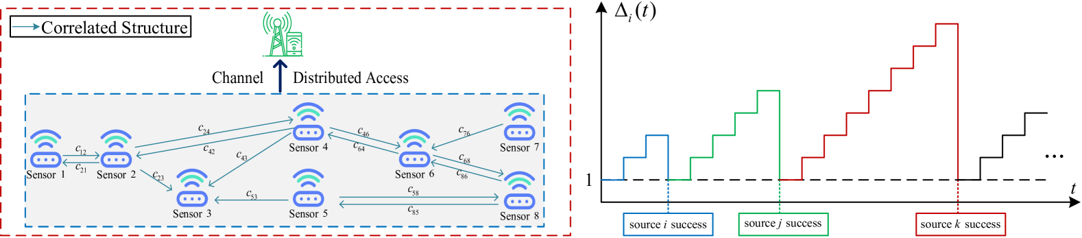
Figure 1: System model for correlated sensors and AoI evolutions of the sensor $i$.

II-A Random Access Network Characterize

As shown in Fig. 1, we consider a status update system consisting of $n$ heterogeneous sensors and one base station, where $n$ sensors observe part of physical processes from the environment, and the base station will play a role in utilizing the transmitted information to estimate the status of the remote system. Generally, we consider using a typical random access protocol, i.e., Slotted Aloha, to adapt large-scale machine-type devices in M2M communications system. In heterogeneous slotted Aloha, the sensor $i$, for $i\in\mathcal{N}=\{1,2,\ldots,n\}$, transmits a status update with probability $q_{i}$. When the transmission fails, the sensor regenerates a new status update with probability $q_{i}$ in the next time slot. In this paper, we adopt the classic collision model in the receiver, i.e., a status update is successfully delivered if and only if there is no concurrent packet transmission in the channel.

We also employ the generate-at-will strategy to manage the status update packets of each sensor, i.e. once a sensor decides to send its status update to the receiver, it generates a fresh status update before the transmission. If the transmission fails, the current status update will be discarded. When the failed sensor retransmits, it generates a new status update. For simplicity, let $a_{i}(t)$ be an indicator variable that denotes whether sensor $i$ successfully transmits the status update to the base station in slot $t$. According to the distributed nature of the access behavior of each slotted Aloha sensor, we have $\Pr\{a_{i}(t)=1\}=p_{i}q_{i}$, and $\Pr\{a_{i}(t)=0\}=1-p_{i}q_{i}$, where $p_{i}$ denotes the successful transmission probability of each Aloha sensor. Under the collision model, a transmission from sensor $i$ is successful if and only if none of the other $n-1$ sensors access the channel. Therefore, $p_{i}$ can be obtained by the following equation

$$p_{i}=\prod_{k\in\mathcal{N}\setminus i}(1-q_{k}).$$ (1)

II-B Age of Information in Correlated Sensors

We leverage Age of Information (AoI) to evaluate the information freshness of the sensors at the base station. AoI measures the time elapsed since the latest received packet at the base station is generated from the sensor, where it grows linearly with time in the absence of new updates at the destination and reduces to the time elapsed since the generation of the delivered status update upon receiving a new status update. A pictorial example of the AoI evolution of the sensor $i$ is given in Fig. 1. Formally, this process can be expressed as

$$\Delta_{i}(t)=t-G_{i}(t),$$ (2)

where $G_{i}(t)$ is the generation time of the latest status update transmitted by sensor $i$ successfully received at the base station at time $t$.

We characterize the correlation structure between sensors using a matrix $\mathbf{C}\in\mathbb{R}^{n\times n}$. At the beginning of each time slot, sensor $i$ captures information about its own state. Additionally, the status update captured by sensor $i$ also includes information about the current state of sensor $j$ with probability $c_{ij}\in[0,1]$, which can occur due to overlapping fields of view between sensors $i$ and $j$ or spatial correlation in the monitored processes. We assume this information sharing or overlap occurs independently for each ordered sensor pair and across time. Consequently, a value of $c_{ij}$ = 0 indicates that sensor $i$ never captures information about sensor $j$, while $c_{ij}=1$ suggests that sensor $i$ has complete details on sensor $j$ at all times. Therefore, the network correlation structure can be described by a matrix C, where each off-diagonal element $c_{ij}$ represents the degree of correlation between sensors. When $c_{ii}=1$ for all sensors in $\mathcal{N}$, each sensor is assumed to always have information about itself. The model also accommodates cases where a sensor intermittently lacks self-information by setting $c_{ii}<1$.

Fig. 1 illustrates an example of a correlated random access network, where sensors capture partial status information from their neighbors and transmit updates to a base station. When sensor $i$ successfully transmits to the base station, it conveys its own state with probability (w.p.) $c_{ii}$ and shares correlated information from other sensors w.p. $c_{ij}$ for $j\in[1,n]$. Consequently, updates received at the base station are often correlated, encompassing data from multiple correlated sensors. For instance, in Fig. 1, when sensor 2 successfully transmits, its update includes its own status w.p. $c_{22}$ and, w.p. $c_{21}$, $c_{23}$, and $c_{24}$, may also incorporate information from sensors 1, 3, and 4, respectively.

Based on the correlation structure described above, the complete AoI evolution of sensor $i$ can be summarized as illustrated in Fig. 1. Both successful transmissions by sensor $i$ and by any other sensor correlated with sensor $i$, e.g., sensor $j$, $k$ in Fig. 1, influence the AoI evolution of sensor $i$.

Let $X_{ij}(t)$ be an indicator variable representing whether the current update at sensor $i$ also captures the information about sensor $j$ in slot $t$. Note that $X_{ij}(t)\sim Bern(c_{ij})$ across pairs $(i,j)$ and independently over time. Given this correlation structure, represented by matrix C, the AoI for sensor $i$ at the base station evolves in the correlated network can be summarized as follows:

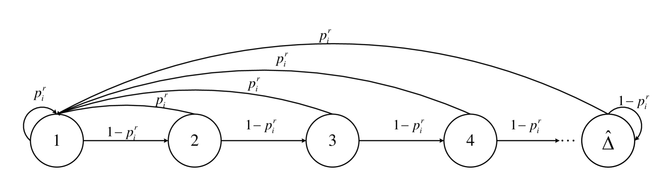
Figure 2: AoI dynamics process of sensor $i$ in the correlated random access network.

$$\Delta_{i}(t+1)=\!\!\left\{\!\!\!\!\!\begin{array}[]{ll}\,\,\,1&\text{if}\,\,\sum_{j=1}^{n}a_{j}(t)X_{ji}(t)=1\\ \,\,\,\min\{\Delta_{i}(t)+1,\hat{\Delta}\}&\text{otherwise,}\end{array}\right.$$ (3)

where the parameter $\hat{\Delta}$ represents the maximum permissible AoI. An upper bound is imposed on AoI because excessively outdated packets are ineffective for time-sensitive applications. The specific value of $\hat{\Delta}$ is finite and determined by the requirements of the given application. According to the description about the indicator variables $a_{i}(t)$ and $X_{ij}(t)$, the evolution of the AoI can be formulated as:

$$\Delta_{i}(t+1)=\left\{\!\!\begin{array}[]{ll}1&\text{w.p.}\,\,p_{i}^{r},\\ \min\{\Delta_{i}(t)+1,\hat{\Delta}\}&\text{w.p.}\,\,1-p_{i}^{r},\end{array}\right.$$ (4)

where $p_{i}^{r}$ denotes the AoI reset probability of sensor $i$. Note that for any sensor successfully transmits, the AoI of the sensor $i$ will be reset w.p. $p_{j}q_{j}c_{ji}$, therefore, the AoI reset probability of sensor $i$ is given by:

$$p_{i}^{r}=\sum_{j=1}^{n}p_{j}q_{j}c_{ji}=\sum_{j=1}^{n}\prod_{k\in\mathcal{N}\setminus i}(1-q_{k})q_{j}c_{ji}.$$ (5)

III Average AoI Analysis And Optimization Problem Formulation

III-A Average Correlated AoI Analysis

According to the AoI dynamics process given in (4), we know that the AoI dynamics of each Aloha sensor can be regarded as a Discrete-Time Markov Renewal Process under a discrete-time Markov chain (DTMC). The embedded Markov chain of each sensor is illustrated in Fig. 2, where the AoI of sensor $i$ resets upon the successful transmission of itself or other correlated sensors; otherwise, it increases by one. The following Lemma presents the steady-state probability distribution of the embedded Markov chain in Fig. 2 and the expression of the long-term average AoI of sensor $i$:

Lemma 1

The steady-state probability distribution of the embedded Markov chain in Fig. 2 can be obtained as:

$$\pi_{i}^{k}=\begin{cases}(1-p_{i}^{r})^{k-1}p_{i}^{r}&k=1,2,\ldots,\hat{\Delta}-1\\ (1-p_{i}^{r})^{k-1}&k=\hat{\Delta}\\ \end{cases}.$$ (6)

where $p_{i}^{r}$ is given by (5), and the long-term average AoI of sensor $i$ is given by:

$$\bar{\Delta}_{i} =\frac{1-(1-p_{i}^{r})^{\hat{\Delta}}}{p_{i}^{r}}$$ (7)

$$=\frac{1-\left(1-\sum_{j=1}^{n}\prod_{k\in\mathcal{N}\setminus i}(1-q_{k})q_{j}c_{ji}\right)^{\hat{\Delta}}}{\sum_{j=1}^{n}\prod_{k\in\mathcal{N}\setminus i}(1-q_{k})q_{j}c_{ji}}.$$

Proof:

See Appendix A. ∎

Finally, the network average AoI, $\bar{\Delta}$, defined as the sum of the AoI values of all nodes [16], is expressed as follows:

$$\bar{\Delta}=\sum_{i=1}^{n}\bar{\Delta}_{i}=\sum_{i=1}^{n}\frac{1-\left(1-\sum_{j=1}^{n}\prod_{k\in\mathcal{N}\setminus i}(1-q_{k})q_{j}c_{ji}\right)^{\hat{\Delta}}}{\sum_{j=1}^{n}\prod_{k\in\mathcal{N}\setminus i}(1-q_{k})q_{j}c_{ji}}.$$ (8)

III-B Problem Formulation

Our objective is to minimize the correlated AoI through the optimal configuration of the transmission probabilities. Specifically, we focus on two specific optimization problems in our paper. The first problem is the individual sensor AoI optimization problem, where only the sensor $i$ is age-sensitive. Thus the problem can then be formulated as follows:

$$~~~~~\min_{q_{i}}\bar{\Delta}_{i},$$ (9)

$$\text{s.t.}\;\;\;q_{i}\in[0,1]$$

The second problem is the aggregate network average AoI optimization problem, where all the sensors are age-sensitive and we aim at minimizing the network average AoI $\bar{\Delta}$ via optimally tuning the transmission probability vector $\boldsymbol{q}$. According to (8), the optimization problem can be defined as

$$~~~~~~\min_{\boldsymbol{q}}\bar{\Delta},$$ (10)

$$\text{s.t.}\;\;\;\boldsymbol{q}\in[0,1]^{n}$$

where $\boldsymbol{q}=(q_{1},\ldots,q_{n})$ denotes the transmission probability vector. According to (7), the aggregate network average AoI optimization problem (10) can be rewritten as follows:

$$\min_{\boldsymbol{q}}\sum_{i=1}^{n}\frac{1-\left(1-\sum_{j=1}^{n}\prod_{m=1,m\neq j}^{n}(1-q_{m})q_{j}c_{ji}\right)^{\hat{\Delta}}}{\sum_{j=1}^{n}\prod_{m=1,m\neq j}^{n}(1-q_{m})q_{j}c_{ji}},$$ (11)

$$~~~~~~~~~~~~~~~~~~~~~~~~~~\text{s.t.}\;\;\;\boldsymbol{q}\in[0,1]^{n}$$

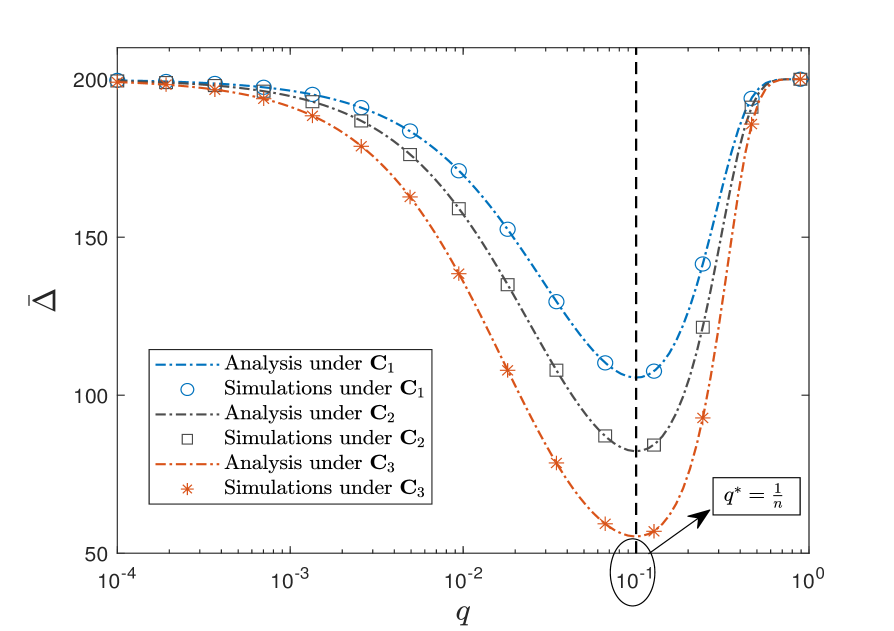
(a)

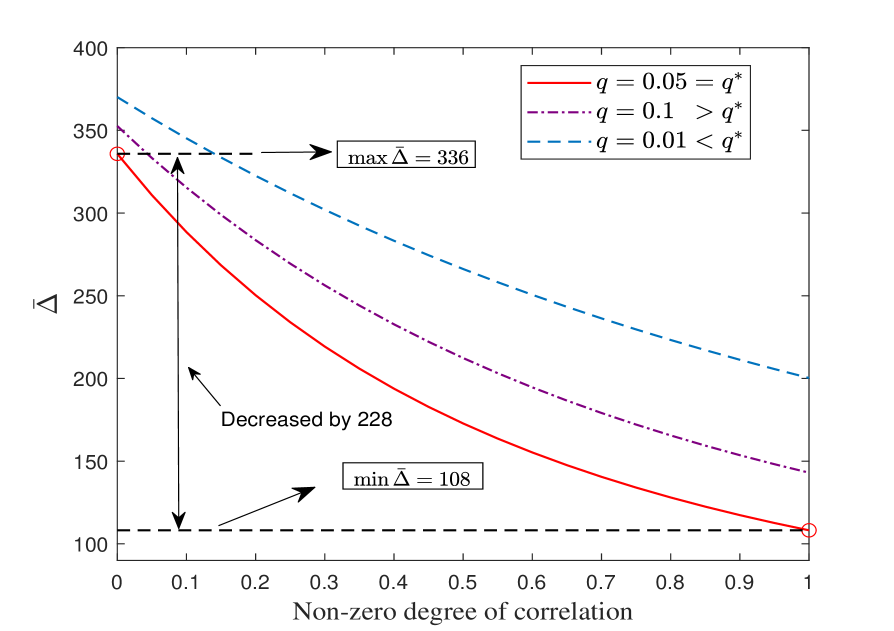
(b)

Figure 3: (a) Network average AoI versus transmission probability $q$ in the homogeneous network under different correlated matrix C, $n=10,\hat{\Delta}=20$. (b) Network average AoI versus varying non-zero degree of correlation $c_{ij}$ in the homogeneous network, $n=20,\hat{\Delta}=20$.

IV Homogeneous AoI Optimization

IV-A Homogeneous Correlated AoI Optimization

We first optimize the AoI in a homogeneous scenario. In this case, the transmission probability of each sensor can be expressed as $q_{i}=q$, where $i=1,\ldots,n$, and the successful transmission probability $p=(1-q)^{n-1}{\overset{n\gg 1}{\approx}}\exp(-nq)$. Moreover, the network average AoI in homogeneous conditions can be simplified as $\bar{\Delta}=n\bar{\Delta}_{i}$, implying that both individual and global optimization are equivalent. The following theorem gives the optimal network average AoI $\bar{\Delta}$ of the homogeneous correlated random access network.

Theorem 1

The optimal network average AoI is given by:

$$\bar{\Delta}^{*}=\sum_{i=1}^{n}\frac{1-\exp\left\{-{\hat{\Delta}\exp(-1)\sum_{j=1}^{n}c_{ji}}\right\}}{\exp(-1)\sum_{j=1}^{n}c_{ji}}.$$ (12)

The corresponding optimal AoI reset probability and the optimal transmission probability of sensor $i$ is given by:

$$p_{i}^{r*}=\exp(-1)\sum_{j=1}^{n}c_{ji},q_{i}^{*}=\frac{1}{n}.$$ (13)

Proof:

See Appendix B. ∎

From Theorem 1, we conclude that although the optimal transmission probability of all sensors is still $q_{i}^{*}=\frac{1}{n}$ in the homogeneous network, both the optimal AoI reset probability $p_{i}^{r*}$ and network average AoI $\bar{\Delta}^{*}$ are improved by the correlated factor $\sum_{j=1}^{n}c_{ji}$. As a result, Theorem 1 explicitly demonstrates that the spatial correlation of sensors can enhance information freshness in random access networks.

IV-B Numerical Result in Homogeneous Network

To better illustrate the impact of the correlated structure, we use three different correlation matrices $\mathbf{C}$ in Fig. 3a, denoted as $\textbf{C}_{1}$, $\textbf{C}_{2}$, and $\textbf{C}_{3}$, respectively. The matrix $\textbf{C}_{1}$ denotes the low-correlation matrix, with diagonal elements $c_{ii}=1$ (i.e., all the sensors have perfect knowledge of itself) and degree of correlation $c_{ij},\forall i\neq j$, set to either 0 or 0.2. The matrices $\textbf{C}_{2}$ and $\textbf{C}_{3}$, referred to as the medium-correlation and high-correlation matrices, respectively, share the same structure as $\textbf{C}_{1}$, but the non-zero degree of correlation 0.2 in $\textbf{C}_{1}$ is replaced by 0.4 and 0.8, respectively.

Additionally, the simulations in Fig. 3a assume the network consisting of $n=10$ sensors, each sampling and transmitting its status update in each time slot with a probability $q_{i}$, where $i=1,\ldots,n$. The maximum permissible AoI for each sensor are set to $\hat{\Delta}=20$ and the simulation runs for $2\times 10^{6}$ time slots. During the simulation, the AoI dynamics of each sensor follow (3). After the simulation, the average AoI for each sensor $\bar{\Delta}_{i}$ and the network average AoI $\bar{\Delta}$ are calculated using (7) and (8), respectively. Both theoretical and simulations result in Fig. 3a illustrate that the network average AoI $\bar{\Delta}$ monotonically decreases when $q<q^{*}$ and monotonically increases when $q>q^{*}$, the optimal network average AoI $\bar{\Delta}^{*}$ therefore is achieved when $q=q^{*}=\frac{1}{n}$.

Fig. 3b illustrates the network average AoI under varying non-zero degrees of correlation $c_{ij}$ in the homogeneous network. To further analyze the performance improvement of correlation on the network’s average AoI, a series C matrices, structured similarly to Fig. 3a with the non-zero degree of correlation $c_{ij}$ varying from 0 to 1, is employed in Fig. 3b. Here, the “same structure” implies that the diagonal elements are also set as $c_{ii}=1$, while the positions of non-zero off-diagonal elements remain unchanged, with only their degrees of correlation varying. The non-zero degree of correlation $c_{ij}$ is corresponding to the x-axis value in Fig. 3b.

Fig. 3a and Fig. 3b clearly demonstrate that, in the homogeneous random access network, the optimal transmission probability can be obtained by Theorem 1. Consequently, regardless of the degree of correlation, when the transmission probability $q$ deviates from the optimal value $q^{*}$, whether higher or lower, the network average AoI $\bar{\Delta}$ increases. Furthermore, regardless of the transmission probability $q$, the network average AoI $\bar{\Delta}$ improves as the degree of correlation increases, and the gap between the network average AoI $\bar{\Delta}$ for different transmission probability $q$ become larger with higher correlation, indicating the exhibition of the correlation gain in random access networks. This gain persists in improving the network AoI even under intense contention conditions resulting from the inherently distributed nature of access behavior.

V Individual Heterogeneous AoI Optimization

V-A Individual Correlated AoI Optimization

In heterogeneous networks, the transmission probability of each sensor is different, i.e., $q_{i}\neq q_{j}$. Let us first consider solving the individual sensor correlated AoI optimization problem defined in (10). The following proposition gives the optimal long-term average AoI $\bar{\Delta}_{i}$ of the sensor $i$.

Proposition 1

The optimal long-term average AoI $\bar{\Delta}_{i}^{*}$ is given by

$$\bar{\Delta}_{i}^{*}=\frac{1-(1-p_{i}^{r*})^{\hat{\Delta}}}{p_{i}^{r*}}$$ (14)

where $p_{i}^{r*}$ represents the optimal AoI reset probability of sensor $i$ in individual optimization and is given by

$$p_{i}^{r*}=\begin{cases}c_{ii}\prod_{k\in\mathcal{N}\setminus i}(1-q_{k})&\text{if }\Omega_{1}\geq\Omega_{2}\\ \\ \sum_{j=1,j\neq i}^{n}q_{j}c_{ji}\prod_{k\in\mathcal{N}\setminus i,j}(1-q_{k})&\text{otherwise}.\\ \end{cases}$$ (15)

where

$$\Omega_{1}=c_{ii}\prod_{k\in\mathcal{N}\setminus i}(1-q_{k}),$$ (16)

and

$$\Omega_{2}=\sum_{j=1,j\neq i}^{n}q_{j}c_{ji}\prod_{m=1,m\neq j,i}^{n}(1-q_{m}).$$ (17)

The corresponding optimal transmission probability $q_{i}^{*}$ in the individual optimization can be obtained as

$$q_{i}^{*}=\mathds{1}(\Omega_{1}\geq\Omega_{2}).$$ (18)

where $\mathds{1}$ is an indicator function, representing $q_{i}^{*}=1\text{ if }\Omega_{1}\geq\Omega_{2}$; otherwise, $q_{i}^{*}=0$.

Proof:

See Appendix C. ∎

In contrast to homogeneous networks, where the transmission probability for all sensors must be uniformly tuned to $q^{*}=\frac{1}{n}$ to minimize the AoI, heterogeneous networks exhibit a different optimal strategy for individual AoI optimization. For sensor $i$, the optimal transmission probability follows a threshold structure influenced by the correlation structure C and the transmission probabilities of the other $n-1$ sensors. The specific threshold is defined in (15)–(17). Here, $\Omega_{1}$ represents the AoI gain achieved through the successful transmission of sensor $i$, while $\Omega_{2}$ reflects the AoI gain contributed by the successful transmission of other $n-1$ sensors.

Unlike homogeneous cases, the optimal transmission probability in heterogeneous networks is not necessarily $\frac{1}{n}$ for every sensor. When the AoI gain contributed by the successful transmission of the other $n-1$ sensors $\Omega_{2}$ is sufficiently high, it may be more beneficial for sensor $i$ to refrain from accessing the channel, in this case, the optimal transmission probability of the sensor $i$ is given as $q_{i}^{*}=0$; otherwise, since individual optimization is considered, sensor $i$ is more inclined to continuously access the channel to deliver its own status updates to optimize its long-term average AoI, in this case, the optimal transmission probability of the sensor $i$ is given as $q_{i}^{*}=1$. Such a threshold-based access structure within certain correlation structures, denoted as C, can help sensors alleviate performance degradation caused by severe contention resulting from the distributed access behavior of the high volume of nodes.

V-B Numerical Results for Individual AoI Optimization

Fig. 4 presents the curve of the long-term average AoI, $\bar{\Delta}_{1}$ for sensor 1 versus the varying non-zero degrees of correlation, $c_{ij}$, under different transmission probability $q_{1}$. The simulation configuration is the same as that in Fig. 3a. In the heterogeneous network, where the transmission probability of each node is different, only sensor 1 is assumed to be age-sensitive. Therefore, Fig. 4 focuses on the AoI evolution of sensor 1 under various parameter settings. Both theoretical and simulations result in Fig. 4a and Fig. 4b indicate that as the non-zero degree of correlation increases, it is advantageous for sensor 1 to reduce its transmission probability. This reduction not only improves the AoI performance of sensor 1, but also mitigates severe conflicts caused by distributed access behaviors in the network. A comparison of Fig. 4a and Fig. 4b reveals that both $q_{1}=0.01$ and $q_{1}=0$ achieve nearly identical AoI performance when there is a strong correlation among sensors. This finding suggests that the transmission probability of the sensor can be significantly reduced, or even set to zero, to minimize its AoI while alleviating network collisions in the correlated random access network.

Fig. 4c presents the individual AoI optimization results outlined in Proposition 1. Assuming that only sensor 1 is age-sensitive, the AoI of sensor 1 can be minimized by following equation (18). As illustrated in Fig. 4c, when $\Omega_{1}\geq\Omega_{2}$, the AoI gain achieved through the successful transmission of sensor 1 outweighs the AoI gain contributed by the successful transmission of the other $n-1$ sensors. Consequently, the optimal transmission probability is set to $q_{1}^{*}=1$ to meet the AoI requirements. Conversely, if $\Omega_{1}\leq\Omega_{2}$, sensor 1 remains silent but can still achieve a minimum AoI due to the high correlation within the network.

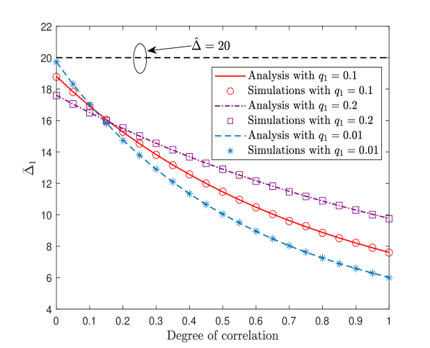
(a)

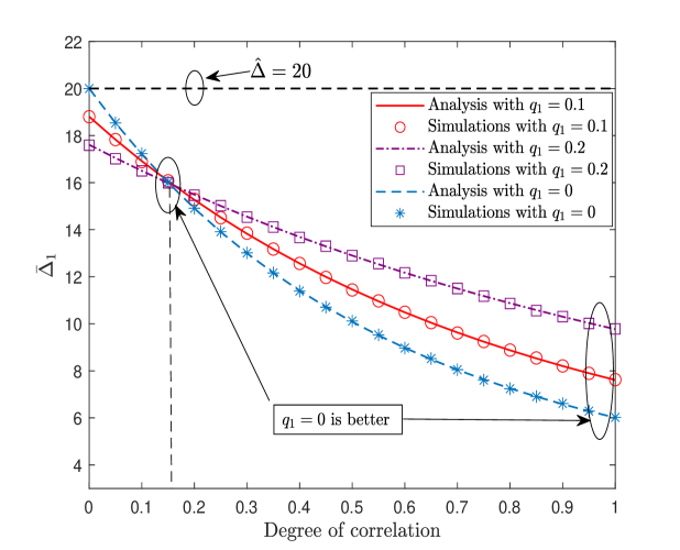
(b)

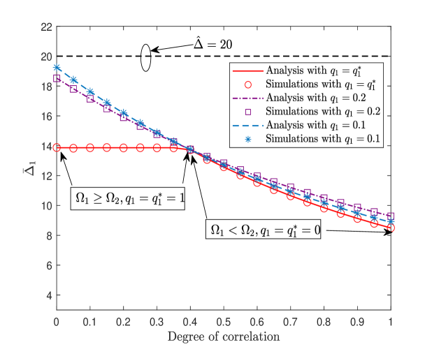
(c)

Figure 4: Long-term average AoI $\bar{\Delta}_{1}$ of the sensor 1 versus non-zero degree of correlation $c_{ij}$ under different $q_{1}$, $n=10,\hat{\Delta}=20,\boldsymbol{q}=[q_{1},q_{2},\ldots,q_{n}]$. (a) $q_{1}=0.01,0.1$ and 0.2, respectively. (b) $q_{1}=0.01,0.1$ and 0, respectively. (c) $q_{1}=0.1,0.3$ and $q_{1}=q_{1}^{*}$, respectively. The other $n-1$ transmission probabilities in $\boldsymbol{q}$ are chosen from [0,0.5] randomly.

VI Global Network Average AoI Optimization

VI-A Aggregate Network Average AoI Optimization

The proposition 1 reveals that the age-sensitive sensor should refrain from transmitting when the AoI gain from its transmission is smaller than the AoI gain achieved by the successful transmission of other related nodes. When all sensors in the correlated network are age-sensitive, optimizing their access behaviors within a specific correlation structure is essential to minimize the network’s average AoI, denoted as $\bar{\Delta}$. We therefore consider solving the global network average AoI optimization problem proposed in (11).

Since the explicit expression of the $\bar{\Delta}$ has been derived, it is intuitive to employ iterative algorithms for calculating the optimal transmission probability vector $\boldsymbol{q}$ of the network sequentially based on the gradient expression of the network average AoI with respect to (w.r.t.) the transmission probability vector $\boldsymbol{q}$, i.e., $\nabla(\bar{\Delta}(\boldsymbol{q}))$.

Note that the network average AoI $\bar{\Delta}$ is determined by the transmission probability vector $\boldsymbol{q}$ and the correlation structure C, the gradient of $\bar{\Delta}$ w.r.t. $\boldsymbol{q}$ is also a vector with $n$ dimensions. We first provide the expression for the partial derivative of $\bar{\Delta}$ concerning any specific transmission probability $q_{k}$

$$\frac{\partial\bar{\Delta}}{\partial q_{k}}=\sum_{i=1}^{n}\left[\frac{\hat{\Delta}\left(1-p_{i}^{r}\right)^{\hat{\Delta}-1}}{p_{i}^{r}}\frac{\partial p_{i}^{r}}{\partial q_{k}}-\frac{\left(1-\left(1-p_{i}^{r}\right)^{\hat{\Delta}}\right)}{(p_{i}^{r})^{2}}\frac{\partial p_{i}^{r}}{\partial q_{k}}\right],$$ (19)

where $k=1,2,\ldots,n$ and $\frac{\partial p_{i}^{r}}{\partial q_{k}}$ is given by

$$\frac{\partial p_{i}^{r}}{\partial q_{k}} =p_{k}c_{ki}-\frac{\sum_{j=1,j\neq k}^{n}q_{j}p_{j}c_{ji}}{1-q_{k}}.$$ (20)

Combining with (19) and (20), the gradient of the network average AoI $\bar{\Delta}$ w.r.t. the transmission probability vector $\boldsymbol{q}$ can be written as follow

$$\nabla(\bar{\Delta}(\boldsymbol{q}))=(\frac{\partial\bar{\Delta}}{\partial q_{1}},\frac{\partial\bar{\Delta}}{\partial q_{2}},\ldots,\frac{\partial\bar{\Delta}}{\partial q_{n}}).$$ (21)

Note that the expressions of $\bar{\Delta}$ and $\nabla(\bar{\Delta}(\boldsymbol{q}))$ contain the $n$ consecutive multiplication terms of the transmission probability $q_{i}$ for $i\in\mathcal{N}$, and the high dimensionality of the transmission probability vector $\boldsymbol{q}$, making the constrained global optimization problem (10) highly non-convex. Therefore, giving the global explicit feasible solution of $\boldsymbol{q}^{*}$ to minimize the network average AoI $\bar{\Delta}$ is still challenging.

To address this, We employ a Multi-Start Projected Adaptive Moment Estimation (MSP-Adam) method to solve the constrained highly non-convex optimization problem (10), ensuring feasible iterates while mitigating local optima issues. Compared to Gradient Descent (GD), Adam enables an adaptive learning rate and is more suitable for optimizing problem (10), which involves the high dimensionality of the transmission probability vector $\boldsymbol{q}$. Although Adam converges quickly, it cannot guarantee convergence to the global optimal solution $\boldsymbol{q}^{*}$ because the optimization problem (10) is highly non-convex. Therefore, the multi-start method is an effective approach to reducing the risk of falling into a local optimum.

To begin with the MSP-Adam method, we first initial $M$ transmission probability vectors, i.e., $\{\boldsymbol{q}_{0}^{(1)},\boldsymbol{q}_{0}^{(2)},\ldots,\boldsymbol{q}_{0}^{(M)}\}$ randomly, learning rate $\eta>0$, maximum iterations $K$, difference tolerance $\epsilon$. For each transmission probability vector, during each iteration, we calculate the current gradient of the network average AoI w.r.t. the transmission probability vector, i.e., $\nabla(\bar{\Delta}(\boldsymbol{q}_{t}))$, upon which we can update the first-order moment vector $\boldsymbol{m}_{t}$ and the second-order moment vector $\boldsymbol{\upsilon}_{t}$ as follow:

$$\begin{cases}\boldsymbol{m}_{t}=\beta_{1}\boldsymbol{m}_{t-1}+(1-\beta_{1})\nabla(\bar{\Delta}(\boldsymbol{q}_{t})),\\ \boldsymbol{\upsilon}_{t}=\beta_{2}\boldsymbol{\upsilon}_{t-1}+(1-\beta_{2})\left(\nabla(\bar{\Delta}(\boldsymbol{q}_{t}))\right)^{2},\\ \hat{\boldsymbol{m}}_{t}=\frac{\boldsymbol{m}_{t}}{1-\beta_{1}},\\ \hat{\boldsymbol{\upsilon}}_{t}=\frac{\boldsymbol{\upsilon}_{t}}{1-\beta_{2}},\end{cases}$$ (22)

where $\beta_{1}$ and $\beta_{2}$ are attenuation factors. Then the transmission probability vector can be updated by:

$$\tilde{\boldsymbol{q}}_{t}=\boldsymbol{q}_{t-1}-\frac{\eta\hat{\boldsymbol{m}}_{t}}{\sqrt{\hat{\boldsymbol{\upsilon}}_{t}}+\delta},$$ (23)

where $\delta$ is a small positive constant to prevent division by zero errors. When $\boldsymbol{q}_{t}$ has been updated, it should be projected onto the feasible region by using:

$$\boldsymbol{q}_{t}=\min(1-\delta,\max(\delta,\tilde{\boldsymbol{q}}_{t})).$$ (24)

Finally, we check whether the new $\boldsymbol{q}$ is convergent using the following equation:

$$\|\boldsymbol{q}_{t}-\boldsymbol{q}_{t-1}\|_{2}\leq\epsilon.$$ (25)

Detail Algorithm methods of the MSP-Adam approach are elaborated in Algorithm 1. According to Algorithm 1, the optimal transmission probability vector $\boldsymbol{q}^{*}$ can be obtained to minimize the network’s average AoI $\bar{\Delta}^{*}$.

Algorithm 1 Multi-Start Projected Adaptive Moment Estimation (MSP-Adam) method

1:Initial learning rate $\eta$, maximum iterations $K$, tolerance $\epsilon$, attenuation factors $\beta_{1}$, $\beta_{2}$ , small enough number $\delta$, and randomly generated $M$ transmission probability vectors $\{\boldsymbol{q}_{0}^{(1)},\boldsymbol{q}_{0}^{(2)},\ldots,\boldsymbol{q}_{0}^{(M)}\}$.

2:$\{\boldsymbol{q}_{0}^{(1)},\boldsymbol{q}_{0}^{(2)},\ldots,\boldsymbol{q}_{0}^{(M)}\}\in[0,1]^{n}$

3:Initialize $\boldsymbol{q}^{*}\leftarrow\emptyset$, $\bar{\Delta}^{*}\leftarrow\infty$

4:for $m=1,2,\ldots,M$ do $\triangleright$ Multi-start initialization

5:  Initialize first and second moment vectors:

$$\boldsymbol{m}_{0}\leftarrow 0,\quad\boldsymbol{v}_{0}\leftarrow 0$$

6:  for $t=1,2,\dots,K$ do $\triangleright$ Adam-based PGD

7:   Compute the gradient based on (19) and (20):

$$\nabla(\bar{\Delta}(\boldsymbol{q}))=(\frac{\partial\bar{\Delta}}{\partial q_{1}},\frac{\partial\bar{\Delta}}{\partial q_{2}},\ldots,\frac{\partial\bar{\Delta}}{\partial q_{n}})$$

8:   Update biased first-moment estimate:

$$\boldsymbol{m}_{t}=\beta_{1}\boldsymbol{m}_{t-1}+(1-\beta_{1})\nabla(\bar{\Delta}(\boldsymbol{q}_{t}))$$

9:   Update biased second-moment estimate:

$$\boldsymbol{\upsilon}_{t}=\beta_{2}\boldsymbol{\upsilon}_{t-1}+(1-\beta_{2})\left(\nabla(\bar{\Delta}(\boldsymbol{q}_{t}))\right)^{2}$$

10:   Correct bias:

$$\hat{\boldsymbol{m}}_{t}=\frac{\boldsymbol{m}_{t}}{1-\beta_{1}^{t}},\quad\hat{\boldsymbol{\upsilon}}_{t}=\frac{\boldsymbol{\upsilon}_{t}}{1-\beta_{2}^{t}},$$

11:   Perform Adam update step:

$$\tilde{\boldsymbol{q}}_{t}=\boldsymbol{q}_{t-1}-\frac{\eta\hat{\boldsymbol{m}}_{t}}{\sqrt{\hat{\boldsymbol{\upsilon}}_{t}}+\delta}$$

12:   Project onto feasible region $[0,1]^{n}$:

$$\boldsymbol{q}_{t}=\min(1-\delta,\max(\delta,\tilde{\boldsymbol{q}}_{t}))$$

13:   if $\|\boldsymbol{q}_{t}-\boldsymbol{q}_{t-1}\|_{2}\leq\epsilon$ then $\triangleright$ Check convergence

14:     break      

15:  Compute objective value $\bar{\Delta}^{(m)}=\bar{\Delta}(\boldsymbol{q}_{t})$

16:  if $\bar{\Delta}^{(m)}<\bar{\Delta}^{*}$ then

17:   Update optimal solution: $\boldsymbol{q}^{*}\leftarrow\boldsymbol{q}_{t}$, $\bar{\Delta}^{*}\leftarrow\bar{\Delta}^{(m)}$   

18:Return $\boldsymbol{q}^{*}$ and $\bar{\Delta}^{*}$

VI-B Complexity and convergence Analysis of MSP-Adam

In this subsection, we analyze the complexity and convergence of the proposed MSP-Adam algorithm. The MSP-Adam algorithm primarily consists of two nested loops. The outer loop (Multi-Start loop) runs $M$ times, each time initializing the optimization from a new random $\boldsymbol{q}$. The inner loop consists of Adam iterations, performing up to $K$ rounds of updates at each starting point. In each Adam iteration, we need to compute the gradient value $\nabla\bar{\Delta}(\boldsymbol{q})$, compute and update the first-moment estimate $\boldsymbol{m}_{t}$ and second-moment estimate $\boldsymbol{\upsilon}_{t}$, update the transmission probability vector $\tilde{\boldsymbol{q}}$, project the $\tilde{\boldsymbol{q}}$ onto the feasible region, and check the convergence of the algorithm based on (25). Consequently, the complexity of each Adam iteration is $\mathcal{O}(n)$. As a result, the overall computational complexity of the MSP-Adam algorithm is $\mathcal{O}(nKM)$, where $M$ is the number of starting points, controlling the global search range; $K$ is the number of Adam iterations at each starting point, influencing the convergence of a single optimization process; and $n$ is the number of the sensors, determining the dimensionality of the optimization problem.

Subsequently, we conduct a detailed analysis of the convergence properties of MSP-Adam in this study. Based on the expression of the network average AoI $\bar{\Delta}$ and its gradient $\nabla\bar{\Delta}(\boldsymbol{q})$ w.r.t. the transmission probability vector $\boldsymbol{q}$, it is evident that $\bar{\Delta}$ is continuously differentiable w.r.t. $\boldsymbol{q}$. Furthermore, $\bar{\Delta}$ is a function mapping satisfies $\mathbb{R}^{n}\rightarrow\mathbb{R}$ and, since each sensor’s long-term average AoI is bounded by $\hat{\Delta}$, the network average AoI $\bar{\Delta}$ is consequently bounded below by $n\hat{\Delta}$. In accordance with [Theorem 2.3] in [41], we can conclude that

$$\lim_{t\to\infty}\|\boldsymbol{q}_{t}-\boldsymbol{q}_{t-1}\|_{2}=0.$$ (26)

Moreover, the multi-start mechanism is a valuable strategy in optimization algorithms, particularly for preventing convergence to local optima. As a result, the MSP-Adam algorithm effectively converges to the optimal solution and consistently yields the optimal transmission probability vector $\boldsymbol{q}^{*}$ which minimizes the network average AoI $\bar{\Delta}$.

Below, we validate the effectiveness of MSP-Adam in obtaining optimal solutions through numerical results. The key presetting parameters of Algorithm 1 are listed in Table I, based on which the optimal transmission probabilities of all the sensors and minimum network average AoI are obtained. Fig. 5 illustrates the network aggregate AoI $\bar{\Delta}$ under different transmission probability vector settings with $n=3$ sensors. In Fig. 5, the optimal $\bar{\Delta}$ is computed exhaustively to establish the AoI lower bound. Meanwhile, the random and homogeneous-optimal mechanisms set the transmission probability vector to a random vector and $\boldsymbol{q}=\mathbf{\frac{1}{n}}$, respectively. The MSP-Adam algorithm, as illustrated in Algorithm 1, is used to obtain the optimal transmission probability vector and the corresponding network’s average AoI. From Fig. 5, we observe that MSP-Adam outperforms the random and homogeneous-optimal mechanisms and converges to the optimal network average AoI $\bar{\Delta}^{*}$ within 10 different correlation scenarios.

TABLE I: Parameter configuration of MSP-Adam.

Parameters	Values
Small positive constant $\delta$	$10^{-8}$
Start points $M$	20
Attenuation factors $\beta_{1},\beta 2$	0.9,0.999
Maximum iterations $K$	$10^{3}$
AoI upper limits of each sensor $\hat{\Delta}$	20
Learning rate $\eta$	0.001
Error tolerance $\epsilon$	$10^{-4}$

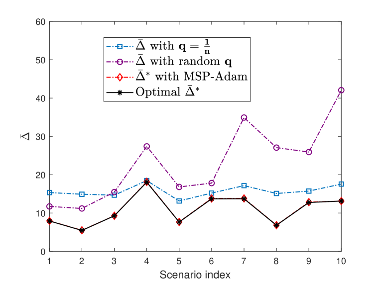
Figure 5: The network average AoI under different transmission probability vector settings with $n=3$ sensors. The correlation matrix C is randomly generated, with off-diagonal elements $c_{ij}$ chosen from the range [0,0.5].

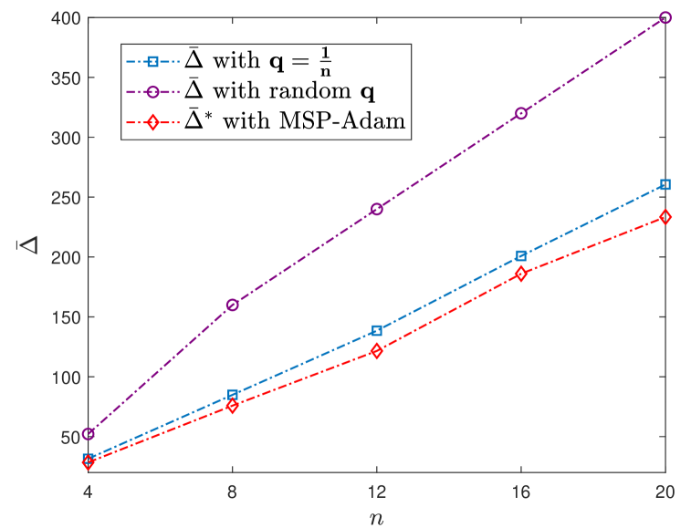
Figure 6: The network average AoI versus the number of sensors $n$ under different transmission probability vector settings. The correlation matrix C is randomly generated, with non-zero off-diagonal elements $c_{ij}$ chosen from the range [0,0.5].

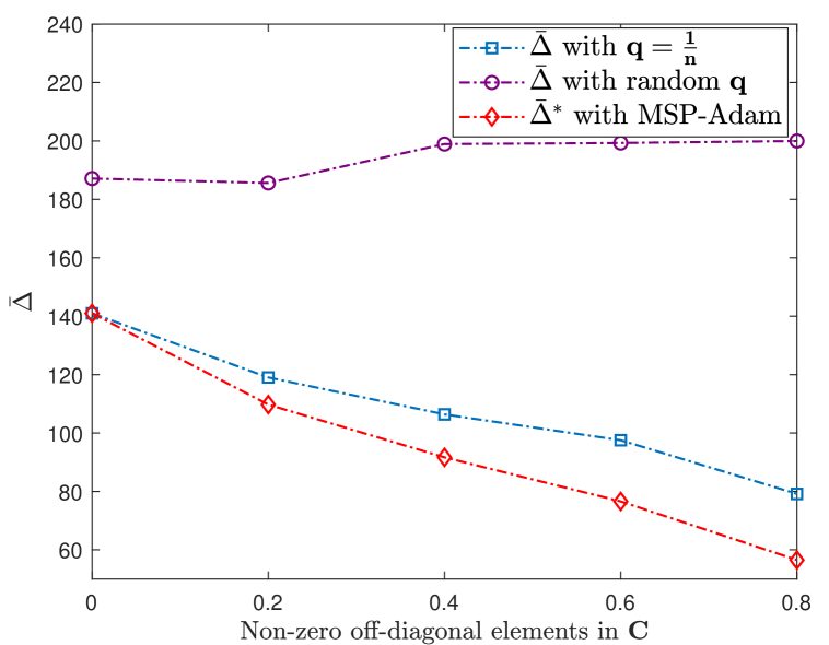
Figure 7: The network average AoI versus the correlation matrix C under different transmission probability vector settings. The number of sensors $n=10$.

TABLE II: The corresponding optimal transmission probability vector $\boldsymbol{q}^{*}$ in Fig. 6 with different number of sensors $n$ under MSP-Adam Algorithm.

optimal solution $\boldsymbol{q}^{*}$	$q_{1}^{*}$	$q_{2}^{*}$	$q_{3}^{*}$	$q_{4}^{*}$	$q_{5}^{*}$	$q_{6}^{*}$	$q_{7}^{*}$	$q_{8}^{*}$	$q_{9}^{*}$	$q_{10}^{*}$	$q_{11}^{*}$	$q_{12}^{*}$	$q_{13}^{*}$	$q_{14}^{*}$	$q_{15}^{*}$	$q_{16}^{*}$	$q_{17}^{*}$	$q_{18}^{*}$	$q_{19}^{*}$	$q_{20}^{*}$
1. $n=4$	0.274	0	0.453	0.274	–	–	–	–	–	–	–	–	–	–	–	–	–	–	–	–
2. $n=8$	0	0.384	0.324	0.049	0	0.243	0	0	–	–	–	–	–	–	–	–	–	–	–	–
3. $n=12$	0	0.372	0.186	0	0.074	0	0	0.158	0	0	0.209	0	–	–	–	–	–	–	–	–
4. $n=16$	0	0	0	0	0.359	0.122	0	0	0	0.129	0	0.188	0	0.200	0	0	–	–	–	–
5. $n=20$	0	0	0	0	0	0.367	0	0	0	0	0	0	0	0	0	0	0.265	0.280	0	0.087

TABLE III: The corresponding optimal transmission probability vector $\boldsymbol{q}^{*}$ in Fig. 7 with different correlated matrix $\mathbf{C}$ under MSP-Adam Algorithm.

optimal solution $\boldsymbol{q}^{*}$	$q_{1}^{*}$	$q_{2}^{*}$	$q_{3}^{*}$	$q_{4}^{*}$	$q_{5}^{*}$	$q_{6}^{*}$	$q_{7}^{*}$	$q_{8}^{*}$	$q_{9}^{*}$	$q_{10}^{*}$
1. $c_{ij}=0$	0.1	0.1	0.1	0.1	0.1	0.1	0.1	0.1	0.1	0.1
2. $c_{ij}=0.2$	0.120	0.711	0	0	0	0.168	0	0	0	0
3. $c_{ij}=0.4$	0	0.415	0	0.235	0	0	0	0	0.350	0
4. $c_{ij}=0.6$	0.142	0.344	0	0	0	0	0	0	0.191	0.322
5. $c_{ij}=0.8$	0	0	0	0	0	0	0.422	0	0.233	0.344

VI-C Numerical Results for MSP-Adam: Performance Analysis

In this subsection, we present the numerical results for the global network average AoI optimization in the heterogeneous network where all sensors are age-sensitive using the MSP-Adam Iteration Algorithm.

Fig. 6 presents a comparison of the global network average AoI optimization versus the number of sensors $n$ using the MSP-Adam algorithm, the optimal homogeneous network setting, and random setting. In Fig, 6, the correlation matrix C is randomly generated, with non-zero off-diagonal elements $c_{ij}$ chosen from the range [0,0.5]. From Fig. 6 we can conclude that when the network scale is small, the performance of the three transmission probability settings is similar, as network competition is not intense at this stage. However, as the network scale increases, the performance gap between the network average AoI under random and homogeneous-optimal settings and that under the MSP-Adam algorithm grows larger, suggesting that in large-scale networks, the performance of network average AoI can be further improved by correlation.

Fig. 7 presents a comparison of the global network average AoI optimization versus the degree of correlation, defined as the values of the non-zero off-diagonal elements in $\mathbf{C}$, using the MSP-Adam algorithm, the optimal homogeneous network setting, and random setting. In Fig. 7, when all off-diagonal elements $c_{ij}=0$, the correlation structure $\mathbf{C}$ in this case is equivalent to the Identity matrix $\mathbf{I}$, indicating that all sensors are independent. In this scenario, the MSP-Adam algorithm achieves an optimal network average AoI that converges to the homogeneous optimal network AoI performance. Consequently, both Fig. 7 and the first row of Table III demonstrate that when there is no correlation between sensors, the optimal transmission probability vector configuration of the network is equivalent to the homogeneous network, i.e., $\boldsymbol{q}^{*}=\mathbf{\frac{1}{n}}$. However, under such a configuration, competition among sensors in the network becomes most intense, as the distributed access behavior and each node shares the same transmission probability.

In contrast to the independent case, as discussed below, the situation changes when considering the correlation between the observations of sensors in the network. Fig. 7 also presents the optimal network average AoI under correlation setting, i.e., when the non-zero off-diagonal elements $c_{ij}$ in correlation matrix $\mathbf{C}$ are not all zero. As Fig. 7 illustrated, in the correlated random access network, the optimal AoI $\bar{\Delta}^{*}$ in both homogeneous and heterogeneous cases can be further optimized. As the degree of correlation increases, the MSP-Adam algorithm reduces the optimal network average AoI, $\bar{\Delta}^{*}$, by 22%, 35%, 45.7%, and 60% compared to the optimal cases in the independent network. Additionally, the gap between the homogeneous-optimal solution and the MSP-Adam algorithm increases, indicating the superior performance of the MSP-Adam method.

Furthermore, both Table II and Table III demonstrate that collisions are significantly reduced in the correlated random access network. For example, in Table II, the network consists of 1, 4, 7, 11, and 16 sensors, respectively, while in Table III, more than 6 sensors prefer to yield the channel to other nodes for transmitting status updates rather than transmitting themselves. This preference increases with the degree of correlation, as the remaining nodes can effectively assist in relaying their status updates to the receiver. As a result, collisions caused by distributed access among sensors can be reduced by at least 25%.

The effectiveness of correlation in improving the average AoI of the network and its impact on the transmission probability of the sensors are fully discussed under different correlation structures $\mathbf{C}$ and the number of sensors $n$, making it possible for sensors to reduce collisions in random access network. The above analysis reveals that the correlation structure in the random access network promotes a more harmonious transmission strategy, which not only improves network AoI performance but also reduces collisions caused by sensor competition.

VII Conclusion

This paper addresses the characterization and optimization of the Age of Information (AoI) in heterogeneous random access networks with correlated sensors, where each sensor has a unique transmission probability and correlation with other sensors. Specifically, we model the AoI dynamics as a discrete-time Markov renewal process using a discrete-time Markov chain (DTMC) and derive the long-term average AoI for each sensor. Furthermore, under the assumption that only one sensor is time-sensitive, we derive the optimal transmission probability for the single sensor in both homogeneous and heterogeneous cases. Additionally, when all sensors are time-sensitive, we propose an iterative algorithm based on the projected gradient descent method to optimize the network average AoI. The algorithm effectively and rapidly converges to the minimum network average AoI while providing the optimal transmission probability vector.

Both theoretical and simulation results demonstrate that when all sensors are independent, the minimum network AoI approaches that of a homogeneous network, with the optimal transmission probability for any sensor given by $q^{*}=\frac{1}{n}$. However, when correlations exist among sensors, the optimal transmission probability for a single sensor follows a threshold-type function. In scenarios where all sensors are time-sensitive, the results of network AoI optimization reveal that the proposed algorithm achieves a robust and harmonious transmission strategy, mitigating performance degradation caused by severe contention in high-density distributed access networks. The algorithm results also reveal that in the heterogeneous correlated random access networks, the competition between sensors will be greatly reduced by 25% and the network average AoI performance can be improved by 22%.

Appendix A Proof of Lemma 1

According to Fig. 2, we have:

$$\begin{cases}\pi_{i}^{1}=p_{i}^{r}\cdot\sum_{k=1}^{\hat{\Delta}}\pi_{i}^{k},\\ \pi_{i}^{k}=(1-p_{i}^{r})\cdot\pi_{i}^{k-1}\text{ for }k=2,3,\ldots,\hat{\Delta}-1,\\ \pi_{i}^{\hat{\Delta}}=(1-p_{i}^{r})\cdot(\pi_{i}^{\hat{\Delta}-1}+\pi_{i}^{\hat{\Delta}})\\ \end{cases}$$ (27)

Note that the following equation always holds:

$$\sum_{k=1}^{\hat{\Delta}}\pi_{i}^{k}=1.$$ (28)

where $p_{i}^{r}$ is given by (5). Combining with (27) and (28), the steady-state distribution of the embedded Markov chain can be obtained. We have the following equation following the definition of the Long-term average AoI:

$$\bar{\Delta}_{i} \overset{\triangle}{=}\lim_{T\to\infty}\sup\frac{1}{T}\sum_{t=0}^{T-1}\Delta_{i}(t)=\sum_{k=1}^{\hat{\Delta}}\pi_{i}^{k}\cdot k$$ (29)

$$=\sum_{k=1}^{\hat{\Delta}-1}(1-p_{i}^{r})^{k-1}p_{i}^{r}k+(1-p_{i}^{r})^{\hat{\Delta}-1}\hat{\Delta}$$

$$=\frac{1-(1-p_{i}^{r})^{\hat{\Delta}}}{p_{i}^{r}}$$

where $p_{i}^{r}$ is given by (5). Therefore, we derive the expression of the long-term average AoI of sensor $i$. The proof of Lemma 1 is completed.

Appendix B Proof of Theorem 1

According to (7), we know that the long-term average AoI $\bar{\Delta}_{i}$ of sensor $i$ is given by:

$$\bar{\Delta}_{i}=\frac{1-(1-p_{i}^{r})^{\hat{\Delta}}}{p_{i}^{r}}\underset{p_{i}^{r}\in(0,1)}{\overset{\hat{\Delta}\gg 1}{\approx}}\frac{1-\exp\left\{-{\hat{\Delta}p_{i}^{r}}\right\}}{p_{i}^{r}}$$ (30)

For simplicity of expression, below we use the approximated expression, i.e.,

$$\bar{\Delta}_{i}=\frac{1-\exp\left\{-{\hat{\Delta}p_{i}^{r}}\right\}}{p_{i}^{r}}.$$ (31)

Note that $\bar{\Delta}_{i}$ is the function of the AoI reset probability of sensor $i$, i.e., $p_{i}^{r}$. Thus we can take the first and second derivatives of $p_{i}^{r}$, which can be written as follows:

$$\bar{\Delta}_{i}^{\prime}=\frac{\partial\bar{\Delta}_{i}}{\partial p_{i}^{r}}=\frac{p_{i}^{r}\hat{\Delta}\exp\left\{-{\hat{\Delta}p_{i}^{r}}\right\}+\exp\left\{-{\hat{\Delta}p_{i}^{r}}\right\}-1}{{p_{i}^{r}}^{2}}.$$ (32)

Since ${p_{i}^{r}}^{2}>0$, we only need to consider the numerator. Let

$$f(p_{i}^{r})=p_{i}^{r}\hat{\Delta}\exp\left\{-{\hat{\Delta}p_{i}^{r}}\right\}+\exp\left\{-{\hat{\Delta}p_{i}^{r}}\right\}-1,$$ (33)

then

$$f^{\prime}(p_{i}^{r})=\frac{\partial f(p_{i}^{r})}{\partial p_{i}^{r}}=-\hat{\Delta}p_{i}^{r}\exp\left\{-{\hat{\Delta}p_{i}^{r}}\right\}.$$ (34)

Note that $0\leq p_{i}^{r}=pq\sum_{j=1}^{n}c_{ji}\leq npq\leq\exp(-1)$ and $\hat{\Delta}\geq 1$, we can obtain that $f^{\prime}(p_{i}^{r})\leq 0$ always holds. Thus we can obtain that $\bar{\Delta}_{i}^{\prime}=\frac{\partial\bar{\Delta}_{i}}{\partial p_{i}^{r}}$ decreases monotonically as $p_{i}^{r}$ increases.

Therefore, the maximum value of $\bar{\Delta}_{i}^{\prime}=\frac{\partial\bar{\Delta}_{i}}{\partial p_{i}^{r}}$ should be obtained when $p_{i}^{r}$ reaches its minimum value. Since we have $0\leq p_{i}^{r}=pq\sum_{j=1}^{n}c_{ji}\leq npq\leq\exp(-1)$, the maximum value of $\bar{\Delta}_{i}^{\prime}$ is given by:

$$\lim_{p_{i}^{r}=0}\bar{\Delta}_{i}^{\prime}~~{\overset{\text{L'Hôpital's Rule}}{=}}~~\frac{\hat{\Delta}-\hat{\Delta}^{2}}{2}\leq 0.$$ (35)

As a result, we have proved that $\bar{\Delta}_{i}^{\prime}\leq 0$ always hold for $\forall{p_{i}^{r}}$. Then we can further obtain that $\bar{\Delta}_{i}$ decreases monotonically as $p_{i}^{r}$ increases, indicating that for any sensor $i$, its correlated AoI is minimized when its corresponding $p_{i}^{r}$ is maximized.

Furthermore, in homogeneous scenario, $p_{i}^{r}=npq\sum_{j=1}^{n}c_{ji}$, and $p=\exp(-nq)$ with a large $n$, we can rewrite the AoI reset probability of sensor $i$ as follows:

$$p_{i}^{r}=nq\exp(-nq)\sum_{j=1}^{n}c_{ji},$$ (36)

where $\sum_{j=1}^{n}c_{ji}$ is a quantity independent of the transmission probability $q$ of the sensor. When the correlation matrix $\mathbf{C}$ is given, $\sum_{j=1}^{n}c_{ji}$ is a constant. Therefore, it is easy to get the optimal transmission probability $q^{*}=\frac{1}{n}$ to maximize the AoI reset probability of sensor $i$ by taking the derivative of $p_{i}^{r}$ to the transmission probability $q$. As a result, the optimal AoI reset probability of sensor $i$ can be obtained as follows:

$$p_{i}^{r*}=\exp(-1)\sum_{j=1}^{n}c_{ji}.$$ (37)

Then we complete the proof of theorem 1.

Appendix C Proof of Proposition 1

From (7) we know that in the heterogeneous network, $p_{i}^{r}$ and $\bar{\Delta}_{i}$ are determined by the transmission probabilities of other $n-1$ sensors. Below we give the expressions for the derivatives of the AoI reset probability $p_{i}^{r}$ and the long-term average AoI $\bar{\Delta}_{i}$ of the sensor $i$ to the transmission probability $q_{i}$:

$$\frac{\partial p_{i}^{r}}{\partial q_{i}} =p_{i}c_{ii}-\frac{\sum_{j=1,j\neq i}^{n}q_{j}p_{j}c_{ji}}{1-q_{i}}$$ (38)

$$=\Omega_{1}-\Omega_{2}.$$

$$\frac{\partial\bar{\Delta}_{i}}{\partial q_{i}}=\left[\frac{\hat{\Delta}\left(1-p_{i}^{r}\right)^{\hat{\Delta}-1}}{p_{i}^{r}}-\frac{\left(1-\left(1-p_{i}^{r}\right)^{\hat{\Delta}}\right)}{(p_{i}^{r})^{2}}\right]\cdot(\Omega_{1}-\Omega_{2}).$$ (39)

where

$$\Omega_{1}=c_{ii}\prod_{m=1,m\neq i}^{n}(1-q_{m}),$$ (40)

and

$$\Omega_{2}=\sum_{j=1,j\neq i}^{n}q_{j}c_{ji}\prod_{m=1,m\neq j,i}^{n}(1-q_{m}).$$ (41)

are two constants in individual optimization, depending only on the correlation structure C and the transmission probabilities of other $n-1$ sensors.

As Appendix B illustrated,

$$\frac{\hat{\Delta}\left(1-p_{i}^{r}\right)^{\hat{\Delta}-1}}{p_{i}^{r}}-\frac{\left(1-\left(1-p_{i}^{r}\right)^{\hat{\Delta}}\right)}{(p_{i}^{r})^{2}}\leq 0.$$ (42)

always holds, indicating that whether the long-term average AoI $\bar{\Delta}_{i}$ is monotonic depends only on the value of $\frac{\partial p_{i}^{r}}{\partial q_{i}}$. As (38) illustrated, in individual optimization, $\frac{\partial p_{i}^{r}}{\partial q_{i}}=\Omega_{1}-\Omega_{2}$ is a constant, depending only on the transmission probabilities of other $n-1$ sensors. When the transmission probabilities of other $n-1$ sensors is given, if $\Omega_{1}\geq\Omega_{2}$, we then have (39) $\leq 0$, $\bar{\Delta}_{i}$ therefore is a monotonically decreasing function of $q_{i}$; otherwise, we have (39) $\geq 0$, $\bar{\Delta}_{i}$ therefore is a monotonically increasing function of $q_{i}$.

As a result, the optimal long-term average AoI $\bar{\Delta}_{i}^{*}$ of sensor $i$ can be obtained as follows:

$$\bar{\Delta}_{i}^{*}=\frac{1-(1-p_{i}^{r*})^{\hat{\Delta}}}{p_{i}^{r*}},$$ (43)

where $p_{i}^{r*}$ is the corresponding optimal AoI reset probability, given by:

$$p_{i}^{r*}=\begin{cases}c_{ii}\prod_{m=1,m\neq i}^{n}(1-q_{m})&\text{if }\Omega_{1}\geq\Omega_{2}\\ \\ \sum_{j=1,j\neq i}^{n}q_{j}c_{ji}\prod_{m=1,m\neq j,i}^{n}(1-q_{m})&\text{otherwise}.\\ \end{cases}$$ (44)

The corresponding optimal transmission probability $q_{i}^{*}$ in the individual optimization can be obtained as:

$$q_{i}^{*}=\mathds{1}(\Omega_{1}\geq\Omega_{2}).$$ (45)

where $\mathds{1}$ is an indicator function, representing $q_{i}^{*}=1\text{ if }\Omega_{1}\geq\Omega_{2}$; otherwise, $q_{i}^{*}=0$. Finally, we complete the proof of Proposition 1.

References

- [1] E. Uysal, O. Kaya, A. Ephremides, J. Gross, M. Codreanu, P. Popovski, M. Assaad, G. Liva, A. Munari, B. Soret, T. Soleymani, and K. H. Johansson, “Semantic communications in networked systems: A data significance perspective,” IEEE Network, vol. 36, no. 4, pp. 233–240, 2022.
- [2] M. Kountouris and N. Pappas, “Semantics-empowered communication for networked intelligent systems,” IEEE Commun. Mag., vol. 59, no. 6, pp. 96–102, June 2021.
- [3] W. Chen, X. Lin, J. Lee, A. Toskala, S. Sun, C. F. Chiasserini, and L. Liu, “5g-advanced toward 6g: Past, present, and future,” IEEE Journal on Selected Areas in Communications, vol. 41, no. 6, pp. 1592–1619, 2023.
- [4] J. Cao, X. Zhu, S. Sun, Z. Wei, Y. Jiang, J. Wang, and V. K. Lau, “Toward industrial metaverse: Age of information, latency and reliability of short-packet transmission in 6g,” IEEE Wireless Communications, vol. 30, no. 2, pp. 40–47, 2023.
- [5] B. Yu, X. Chen, and Y. Cai, “Age of information for the cellular internet of things: Challenges, key techniques, and future trends,” IEEE Commun. Mag., vol. 60, no. 12, pp. 20–26, 2022.
- [6] S. Kaul, R. Yates, and M. Gruteser, “Real-time status: How often should one update?” in 2012 Proceedings IEEE INFOCOM. IEEE, 2012, pp. 2731–2735.
- [7] R. Talak, S. Karaman, and E. Modiano, “Optimizing information freshness in wireless networks under general interference constraints,” IEEE/ACM Transactions on Networking, vol. 28, no. 1, pp. 15–28, 2020.
- [8] R. Talak, I. Kadota, S. Karaman, and E. Modiano, “Scheduling policies for age minimization in wireless networks with unknown channel state,” in 2018 IEEE International Symposium on Information Theory (ISIT), 2018, pp. 2564–2568.
- [9] R. Talak, S. Karaman, and E. Modiano, “Improving age of information in wireless networks with perfect channel state information,” IEEE/ACM Transactions on Networking, vol. 28, no. 4, pp. 1765–1778, 2020.
- [10] B. Zhou and W. Saad, “Minimum age of information in the internet of things with non-uniform status packet sizes,” IEEE Transactions on Wireless Communications, vol. 19, no. 3, pp. 1933–1947, 2020.
- [11] I. Kadota, A. Sinha, E. Uysal-Biyikoglu, R. Singh, and E. Modiano, “Scheduling policies for minimizing age of information in broadcast wireless networks,” IEEE/ACM Transactions on Networking, vol. 26, no. 6, pp. 2637–2650, 2018.
- [12] M. A. Abd-Elmagid, H. S. Dhillon, and N. Pappas, “A reinforcement learning framework for optimizing age of information in rf-powered communication systems,” IEEE Transactions on Communications, vol. 68, no. 8, pp. 4747–4760, 2020.
- [13] J. Sun, L. Wang, Z. Jiang, S. Zhou, and Z. Niu, “Age-optimal scheduling for heterogeneous traffic with timely throughput constraints,” IEEE Journal on Selected Areas in Communications, vol. 39, no. 5, pp. 1485–1498, 2021.
- [14] C. Li, Q. Liu, S. Li, Y. Chen, Y. T. Hou, W. Lou, and S. Kompella, “Scheduling with age of information guarantee,” IEEE/ACM Transactions on Networking, vol. 30, no. 5, pp. 2046–2059, 2022.
- [15] H. Hu, K. Xiong, H.-C. Yang, Q. Ni, B. Gao, P. Fan, and K. B. Letaief, “Aoi-minimal online scheduling for wireless-powered iot: A lyapunov optimization-based approach,” IEEE Transactions on Green Communications and Networking, vol. 7, no. 4, pp. 2081–2092, 2023.
- [16] H. H. Yang, C. Xu, X. Wang, D. Feng, and T. Q. Quek, “Understanding age of information in large-scale wireless networks,” IEEE Transactions on Wireless Communications, vol. 20, no. 5, pp. 3196–3210, May 2021.
- [17] H. H. Yang, A. Arafa, T. Q. S. Quek, and H. V. Poor, “Spatiotemporal analysis for age of information in random access networks under last-come first-serve with replacement protocol,” IEEE Transactions on Wireless Communications, vol. 21, no. 4, pp. 2813–2829, 2022.
- [18] X. Sun, F. Zhao, H. H. Yang, W. Zhan, X. Wang, and T. Q. S. Quek, “Optimizing age of information in random-access poisson networks,” IEEE Internet of Things Journal, vol. 9, no. 9, pp. 6816–6829, 2022.
- [19] F. Zhao, X. Sun, W. Zhan, X. Wang, J. Gong, and X. Chen, “Age-energy tradeoff in random-access poisson networks,” IEEE Transactions on Green Communications and Networking, vol. 6, no. 4, pp. 2055–2072, 2022.
- [20] F. Zhao, N. Pappas, C. Ma, X. Sun, T. Q. S. Quek, and H. H. Yang, “Age-threshold slotted aloha for optimizing information freshness in mobile networks,” IEEE Transactions on Wireless Communications, vol. 23, no. 11, pp. 17 236–17 251, 2024.
- [21] J. Sun, Z. Jiang, B. Krishnamachari, S. Zhou, and Z. Niu, “Closed-form whittle’s index-enabled random access for timely status update,” IEEE Transactions on Communications, vol. 68, no. 3, pp. 1538–1551, 2020.
- [22] A. Maatouk, M. Assaad, and A. Ephremides, “On the age of information in a csma environment,” IEEE/ACM Transactions on Networking, vol. 28, no. 2, pp. 818–831, 2020.
- [23] R. D. Yates and S. K. Kaul, “Status updates over unreliable multiaccess channels,” in 2017 IEEE International Symposium on Information Theory (ISIT), 2017, pp. 331–335.
- [24] W. Zhan and L. Dai, “Massive random access of machine-to-machine communications in lte networks: Modeling and throughput optimization,” IEEE Transactions on Wireless Communications, vol. 17, no. 4, pp. 2771–2785, 2018.
- [25] W. Zhan, D. Wu, X. Sun, Z. Guo, P. Liu, and J. Liu, “Peak age of information optimization of slotted aloha: Fcfs versus lcfs,” IEEE Transactions on Network Science and Engineering, vol. 10, no. 6, pp. 3719–3731, 2023.
- [26] D. C. Atabay, E. Uysal, and O. Kaya, “Improving age of information in random access channels,” in IEEE INFOCOM 2020 - IEEE Conference on Computer Communications Workshops (INFOCOM WKSHPS), 2020, pp. 912–917.
- [27] O. T. Yavascan and E. Uysal, “Analysis of slotted aloha with an age threshold,” IEEE Journal on Selected Areas in Communications, vol. 39, no. 5, pp. 1456–1470, 2021.
- [28] X. Chen, K. Gatsis, H. Hassani, and S. S. Bidokhti, “Age of information in random access channels,” IEEE Transactions on Information Theory, vol. 68, no. 10, pp. 6548–6568, 2022.
- [29] J. Wang, J. Yu, X. Chen, L. Chen, C. Qiu, and J. An, “Age of information for frame slotted aloha,” IEEE Transactions on Communications, vol. 71, no. 4, pp. 2121–2135, 2023.
- [30] H. Zhang, Z. Jiang, S. Xu, and S. Zhou, “Error analysis for status update from sensors with temporally and spatially correlated observations,” IEEE Transactions on Wireless Communications, vol. 20, no. 3, pp. 2136–2149, 2021.
- [31] J. Hribar, M. Costa, N. Kaminski, and L. A. DaSilva, “Using correlated information to extend device lifetime,” IEEE Internet of Things Journal, vol. 6, no. 2, pp. 2439–2448, 2019.
- [32] J. Hribar, A. Marinescu, A. Chiumento, and L. A. Dasilva, “Energy-aware deep reinforcement learning scheduling for sensors correlated in time and space,” IEEE Internet of Things Journal, vol. 9, no. 9, pp. 6732–6744, 2022.
- [33] Q. He, G. Dán, and V. Fodor, “Joint assignment and scheduling for minimizing age of correlated information,” IEEE/ACM Transactions on Networking, vol. 27, no. 5, pp. 1887–1900, 2019.
- [34] B. Zhou and W. Saad, “On the age of information in internet of things systems with correlated devices,” in GLOBECOM 2020 - 2020 IEEE Global Communications Conference, 2020, pp. 1–6.
- [35] A. E. Kalør and P. Popovski, “Minimizing the age of information from sensors with common observations,” IEEE Wireless Communications Letters, vol. 8, no. 5, pp. 1390–1393, 2019.
- [36] Tripathi, Vishrant and Modiano, Eytan, “Optimizing age of information with correlated sources,” in Proc. ACM MobiHoc, 2022, pp. 41–50.
- [37] V. Tripathi and E. Modiano, “Optimizing Age of Information With Correlated Sources,” IEEE/ACM Transactions on Networking, pp. 1–16, 2024.
- [38] J. Tong, L. Fu, and Z. Han, “Age-of-information oriented scheduling for multichannel iot systems with correlated sources,” IEEE Transactions on Wireless Communications, vol. 21, no. 11, pp. 9775–9790, 2022.
- [39] R. V. Ramakanth, V. Tripathi, and E. Modiano, “Monitoring correlated sources: Aoi-based scheduling is nearly optimal,” IEEE Transactions on Mobile Computing, pp. 1–12, 2024.
- [40] Ramakanth, R Vallabh and Tripathi, Vishrant and Modiano, Eytan, “Monitoring Correlated Sources: AoI-based Scheduling is Nearly Optimal,” in IEEE INFOCOM 2024 - IEEE Conference on Computer Communications, 2024, pp. 641–650.
- [41] P. H. Calamai and J. J. Moré, “Projected gradient methods for linearly constrained problems,” Mathematical programming, vol. 39, no. 1, pp. 93–116, 1987.