Transient and steady convection in two dimensions

Abstract

We simulate thermal convection in a two-dimensional square box using the no-slip condition on all boundaries, and isothermal bottom and top walls and adiabatic sidewalls. We choose 0.1 and 1 for the Prandtl number and vary the Rayleigh number between $10^{6}$ and $10^{12}$. We particularly study the temporal evolution of integral transport quantities towards their steady states. Perhaps not surprisingly, the velocity field evolves more slowly than the thermal field. Its steady state is nominal in the sense that large-amplitude low-frequency oscillations persist around plausible averages. We study these oscillation characteristics.

1 Introduction

Turbulent flows driven by buoyancy due to inhomogeneity of the temperature are common in nature and applications (Verma, 2018; Schumacher & Sreenivasan, 2020; Lohse & Shishkina, 2023). Rayleigh-Bénard convection (RBC) is a paradigm for such flows. The RBC originally referred to shallow horizontally extended layers of fluid, heated from below and cooled from above, and the horizontal walls are smooth unless otherwise specified. In this traditional paradigm, RBC is entirely governed by Prandtl and Rayleigh numbers—where the Prandtl number $Pr$ is the ratio of the kinematic viscosity $\nu$ to the thermal diffusivity $\kappa$ of the fluid, and the Rayleigh number $Ra$ is the ratio of the forcing strength to the dissipative mechanisms. Heat and momentum transport across the convective fluid layer are two global responses to thermal driving in RBC. Heat transport is measured by the Nusselt number $Nu$, which is the total heat flux relative to that by conduction in the absence of fluid motion, and the momentum transport by an appropriate Reynolds number $Re$, which defines the flow strength.

Because the Rayleigh number is proportional to $H^{3}$, where $H$ is the height of the convection apparatus, there has been a tendency in the last 25 or so years to choose as high a value of $H$ as possible while, by necessity, shrinking the horizontal dimension (e.g., Castaing et al. (1989); Niemela et al. (2000)). The same is also true of direct numerical simulations (DNS) (e.g., Stevens et al. (2011); Iyer et al. (2020)). The choice of a low aspect ratio $\Gamma\equiv L/H$ (where $L$ is the horizontal dimension of the apparatus) is common in the quest to achieve very high Rayleigh numbers, but an organized motion that develops in such flows has its own structural morphology (Kadanoff, 2001; Sreenivasan et al., 2002; Chillà & Schumacher, 2012; Foroozani et al., 2014, 2017; Verma et al., 2017) that depends on the aspect ratio and the shape of the apparatus; see also Pandey et al. (2022a); Stevens et al. (2024). Pure scaling laws in such flows are unlikely for all conditions, yet it is common to fit the Nusselt and Reynolds numbers by power laws with respect to $Ra$, i.e., $Nu\sim Ra^{\gamma}$ and $Re\sim Ra^{\zeta}$. As pointed out by Doering (2020), fitting such local exponents for small ranges of data is bound to lead to conclusions of uncertain value. Indeed, there are considerable variations of the effective exponents $\gamma$ and $\zeta$ from one study to another, and have been the subject of extensive reviews—e.g., by Chillà & Schumacher (2012); Lohse & Shishkina (2024). In a series of large simulations, an effort has been made to avoid the constraining effect of the sidewalls by stipulating periodic boundary conditions on them (Samuel et al., 2024). These studies mimicking large aspect ratio convection have revealed a very different nature of near-wall velocity from a traditional boundary layer that undergoes laminar-turbulent transition, and have implications for the so-called ultimate state.

There has been the expectation that the riddle of the ultimate state can be solved for the two-dimensional (2D) case in which the flow is compelled to occur only in a vertical plane (Zhu et al., 2018; Samuel & Verma, 2024; Tiwari et al., 2025) because of the natural hope that very high Rayleigh numbers can be achieved here for the same computing power. Existing data show a heat transport scaling that is similar to the three-dimensional (3D) counterpart (Schmalzl et al., 2004; van der Poel et al., 2013; Pandey et al., 2016; Zhang et al., 2017; Pandey, 2021) but the Nusselt number in 2D is smaller when $Pr\geq 1$ (van der Poel et al., 2013), although essentially the same when $Pr$ is small (Pandey, 2021), as for liquid metals. The Reynolds number, on the other hand, shows very different behaviors in 2D and 3D. The magnitudes of momentum transport and the scaling exponent $\zeta$ are consistently higher in 2D, with $\zeta\geq 0.60$ (Schmalzl et al., 2004; van der Poel et al., 2013; Zhang et al., 2017; Pandey, 2021). As a summary, the exponent $\gamma$ has been reported to take values in the range [1/4, 1/3], while $\zeta$ assumes values in the range [4/9, 2/3] (Verma, 2018). Note that these scaling features are well captured by the model of Grossmann and Lohse (Grossmann & Lohse, 2000); see also Pandey et al. (2016).

In this paper, we perform DNS of 2D convection in a unit box for $Pr=0.1$ and $Pr=1$, for Rayleigh numbers between $10^{6}$ and $10^{12}$, not only for the purposes of exploring flow properties but also for highlighting the challenges of simulating 2D convection. We use the no-slip condition on all boundaries, with bottom and top walls isothermal and sidewalls adiabatic. In particular, we show that the velocity field evolves more slowly than the temperature, and call attention to large fluctuations that occur in what may be regarded effectively as the steady state of the velocity field. We relate these fluctuations to heat transport characteristics and provide estimates of suitably defined transient times. Heat transport also exhibits persistently wild fluctuations about its mean for strong thermal forcing. The main qualitative conclusion of this study is that such long transients, as well as wildly fluctuating heat transport, at least for aspect ratios of order unity, make the observation of the so-called ultimate state as elusive in 2D (Doering et al., 2019) as in 3D (Doering, 2020).

2 Numerical methodology

We perform direct numerical simulations in a 2D fluid layer with horizontal dimension $L$, with an imposed temperature difference $\Delta T$ between the bottom and top plates separated by vertical dimension $H$. For this work, the aspect ratio $\Gamma=L/H=1$. The following Oberbeck-Boussinesq equations dictating the flow are solved using Nek5000 solver :

$$\nabla\cdot{\bm{u}} = 0,$$ (1)

$$\frac{\partial{\bm{u}}}{\partial t}+{\bm{u}}\cdot\nabla{\bm{u}} = -\frac{\nabla p}{\rho_{0}}+\alpha g(T-T_{0})\hat{z}+\nu\nabla^{2}{\bm{u}},$$ (2)

$$\frac{\partial T}{\partial t}+{\bm{u}}\cdot\nabla T = \kappa\nabla^{2}T.$$ (3)

Here, ${\bm{u}}=(u_{x},u_{z})$, $p$, and $T$ are the velocity, pressure, and temperature, respectively; $\rho_{0}$ is the reference density and $T_{0}$ is the reference temperature. We non-dimensionalize equations (1)–(3) using $H$, $\Delta T$, $u_{\mathrm{f}}$, and $t_{\mathrm{f}}$ as the scales for length, temperature, velocity, and time, respectively, where $u_{\mathrm{f}}=\sqrt{\alpha g\Delta TH}$ is the free-fall velocity and $t_{\mathrm{f}}=H/u_{\mathrm{f}}$ is the free-fall time. The result contains the Prandtl number $Pr$ and the Rayleigh number $Ra=\alpha g\Delta TH^{3}/(\nu\kappa)$, where $\alpha$ is the isobaric thermal expansion coefficient and $g$ is the acceleration due to gravity. We explore two fluids with $Pr=0.1$ and $Pr=1$ for $Ra$ between $10^{6}$ and $10^{12}$. The square domain is decomposed into $N_{e}$ elements, and each element is further resolved using Lagrangian interpolation polynomials of order $N$ in both horizontal and vertical directions. Thus, the entire flow is resolved using $N_{e}N^{2}$ mesh cells. The no-slip condition for the velocity field is imposed on all boundaries. Isothermal and adiabatic conditions for the temperature field are imposed on the horizontal plates and sidewalls, respectively. The crucial simulation parameters are summarized in table 1 of Appendix A.

To resolve the thermal and viscous boundary layers, finer mesh is used near all boundaries. The spatial resolution in the flow is further ensured by computing the Kolmogorov length scale $\eta$, which is nominally the finest scale in the velocity field, and stipulating that the local vertical grid spacing $\Delta_{z}(z)$/$\eta(z)<1.5$ for all simulations. Note that the kinetic energy dissipation rate is defined as

$$\varepsilon_{u}(\bm{x})=\frac{\nu}{2}\sum_{l,m}\left(\frac{\partial u_{l}}{\partial x_{m}}+\frac{\partial u_{m}}{\partial x_{l}}\right)^{2}$$ (4)

with $l,m=(x,z)$, and the local Kolmogorov scale being given by $\eta=(\nu^{3}/\varepsilon_{u})^{1/4}$. As the intermittent variation of $\varepsilon_{u}(\bm{x})$ in the flow leads to variations in the Kolmogorov scale as well, we estimate an average Kolmogorov scale in each horizontal plane using the horizontally- and temporally-averaged dissipation as

$$\eta(z)=\frac{\nu^{3/4}}{\langle\varepsilon_{u}\rangle_{x,t}^{1/4}(z)}.$$ (5)

The finest length scale in the temperature field, the Batchelor scale $\eta/\sqrt{Pr}$, is of the same order as $\eta$, or coarser, in the present work. Thus, it is always adequately resolved.

3 Other associated definitions

The Nusselt number in a horizontal plane is computed as (Chillà & Schumacher, 2012)

$$Nu(z)=\frac{\langle u_{z}T\rangle_{x,t}-\kappa\partial\langle T\rangle_{x,t}/\partial z}{\kappa\Delta T/H},$$ (6)

where $\langle u_{z}T\rangle_{x,t}$ is the convective component of the heat flux and $-\kappa\partial\langle T\rangle_{x,t}/\partial z$ is the diffusive component. As the vertical velocity vanishes at the horizontal plates, this relation yields the definition using the wall temperature gradient, as

$$Nu_{\partial_{z}T}=-\frac{H}{\Delta T}\left.\frac{\partial\langle T\rangle_{x,t}}{\partial z}\right|_{z=0,H}\,.$$ (7)

Averaging equation (6) along the vertical direction yields the following relation for the global heat transport across the convective layer:

$$Nu=1+\frac{H}{\kappa\Delta T}\langle u_{z}T\rangle_{A,t}\,.$$ (8)

Here $\langle\cdot\rangle_{A,t}$ stands for the average over the entire flow domain and simulation time covering the steady state.

In another family of relations, the exact relations in RBC (Howard, 1972; Shraiman & Siggia, 1990) connect the Nusselt number $Nu$ with the globally-averaged kinetic energy dissipation rate $\varepsilon_{u}$ and the thermal dissipation rate $\varepsilon_{T}$, as

$$\langle\varepsilon_{u}\rangle_{A,t} = \frac{\nu^{3}}{H^{4}}\frac{(Nu-1)Ra}{Pr^{2}}\,,$$ (9)

$$\langle\varepsilon_{T}\rangle_{A,t} = \kappa\frac{(\Delta T)^{2}}{H^{2}}Nu.$$ (10)

Here, the thermal dissipation rate $\varepsilon_{T}=\kappa(\partial T/\partial x_{j})^{2}$ is the rate of thermal energy loss per unit mass. Thus, the Nusselt number can also be estimated from mean dissipation rates:

$$Nu_{\varepsilon_{u}} = 1+\frac{H^{4}}{\nu^{3}}\frac{Pr^{2}}{Ra}\langle\varepsilon_{u}\rangle_{A,t}\,,$$ (11)

$$Nu_{\varepsilon_{T}} = \frac{H^{2}}{(\Delta T)^{2}}\frac{\langle\varepsilon_{T}\rangle_{A,t}}{\kappa}.$$ (12)

The agreement among simulated values from different definitions serves as a check on the accuracy and the adequacy of spatial and temporal resolutions (Stevens et al., 2010; Zhang et al., 2017; Pandey et al., 2022a). In the following, we discuss the approach to stationarity of the Nusselt number results using these definitions and relations, with comments on the scaling of global averages. In equations (6)–(8) and (11)–(12), the Nusselt numbers are globally averaged quantities, though we do not show the averaging symbol explicitly, following standard usage of the past.

4 Transient characteristics

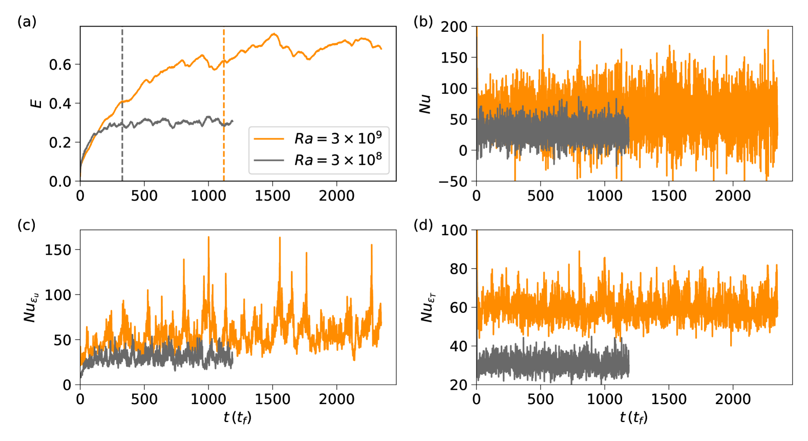
Figure 1: Evolution of the integral quantities in the transient state for $Pr=0.1$, and $Ra=3\times 10^{8}$ (black curves) and $Ra=3\times 10^{9}$ (orange curves). (a) The domain-averaged kinetic energy $E(t)$ increases slowly and takes a few thousand free-fall times to reach the steady state. The transient time is longer for higher $Ra$. Dashed vertical lines show a quantitative measure of the transient time $t_{\mathrm{trns}}$, obtained from equation (15), to be discussed later. Panels (b), (c) and (d) show that the Nusselt number fluctuates rapidly about its mean nearly from the start, but fluctuations have different characters depending on the definition of the Nusselt number. In (b), the fluctuations in $Nu(t)$ are strong and of high frequency with no well-defined transient state, and there is an overlap for the two $Ra$. (c) shows that one can roughly identify a transient state in $Nu_{\varepsilon_{u}}(t)$, which exhibits very strong fluctuations containing both high and low frequencies. (d) shows that $Nu_{\varepsilon_{T}}(t)$ fluctuates similar to $Nu(t)$ in (b), but there is no overlap for the two Rayleigh numbers.

A common method for initiating high-$Ra$ simulations is to start them from the flow at a lower $Ra$. Simulations can also be performed ab initio from the conduction state with random perturbations. In both cases, global heat flux and kinetic energy evolve with time, and one needs to wait some time before a statistically steady state is attained. Figure 1 shows the temporal evolution of integral quantities for the two $Ra$ indicated and $Pr=0.1$, with simulations initiated from the conduction state. On the one hand, we observe that $Nu$ and $Nu_{\varepsilon_{T}}$ in figure 1(b,d) start oscillating about some mean value shortly after the simulation begins. On the other hand, $Nu_{\varepsilon_{u}}$ in figure 1(c) initially increases and starts to fluctuate about a mean value only after some time has elapsed. The instantaneous domain-averaged kinetic energy $E=\langle(u_{x}^{2}+u_{z}^{2})/2\rangle_{A}$ in figure 1(a) offers the best means to determine the time to the steady state. There is no ambiguity about this approach for the lower $Ra$; however, aside from the fact that it takes longer at the higher $Ra$ for the energy to achieve its steady state, the latter is somewhat nominal because fluctuations about the average are significant. The situation becomes more so at even higher Rayleigh numbers. Fluctuations in the domain-averaged energy $E$ follow from dynamical considerations; we shall show this in § 6.

We define the average kinetic energy in the steady state, $E_{\mathrm{av}}$, as

$$E_{\mathrm{av}}=\frac{1}{2}u_{\mathrm{RMS}}^{2}/u_{\mathrm{f}}^{2}\,,$$ (13)

where $u_{\mathrm{RMS}}=\sqrt{\langle u_{x}^{2}+u_{z}^{2}\rangle_{A,t}}$ is the root mean square (RMS) velocity of the flow in the steady state, and plot it in figure 2 as a function of $Ra$. Before discussing differences between the two Prandtl numbers, we note the major difference between 2D and 3D fluctuations. In the 3D case, for low and moderate Prandtl numbers, $E_{\mathrm{av}}$ is a slowly decreasing function of $Ra$; for example, $E_{\mathrm{av}}$ from a horizontally periodic cuboid of $\Gamma=4$ for $Pr=0.7$ (from Samuel et al. (2024)), shown as green squares in figure 2, follows a $Ra^{-0.07}$ scaling. The corresponding behavior for 2D cases is that the fluctuations increase with $Ra$. The behavior is different for different $Pr$ when the Rayleigh numbers are low, but follows a roughly $Ra^{1/3}$ scaling at high Rayleigh numbers, as indicated by the blue and red dashed lines in figure 2. The challenges posed by this increasing trend will be discussed below.

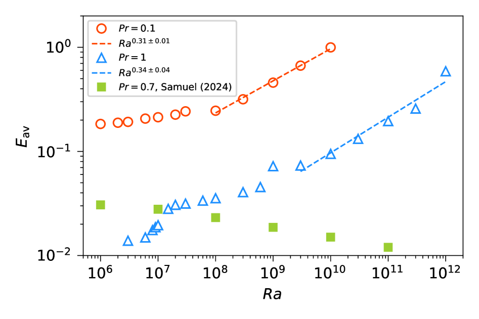
Figure 2: Global (area- as well as time-averaged) kinetic energy in the steady state $E_{\mathrm{av}}$ as a function of $Ra$. An increasing trend with $Ra$ is observed in 2D RBC. In the turbulent regimes ($Ra>10^{8}$ for $Pr=0.1$ and $Ra>10^{10}$ for $Pr=1$), the data roughly follow $E_{\mathrm{av}}\sim Ra^{1/3}$, shown as dashed lines. In contrast, $E_{\mathrm{av}}$ in 3D RBC for $Pr=0.7$ (taken from Samuel et al. (2024)) shows a weakly decreasing trend. The transition observed in these figures, at least for $Pr=1$, is related to a crossover in the large structure from a two-cell configuration to a single cell. The statistical error bars in almost all the figures here are comparable to the thickness of the symbols. The exception is figure 6 for which the errors bars are shown explicitly.

It is useful to study the variation of $t_{\mathrm{trns}}$ (which is the time required for $E(t)$ to attain some stipulated fraction of $E_{\mathrm{av}}$) with respect to $Ra$ and $Pr$ by some simple scheme. To this end, we plot the evolution of $E(t)$ for $Ra=3\times 10^{9}$ and $Ra=10^{10}$ for $Pr=0.1$ in figure 3. The growth of $E$ for both $Ra$ is comparable for initial times but the curve for higher $Ra$ continues to grow for a longer period before a nominally steady state is reached, but with conspicuous fluctuations.

Figure 3: Evolution of the domain-averaged kinetic energy $E(t)$ in the transient state for $Pr=0.1$ and $Ra=3\times 10^{9}$ and $Ra=10^{10}$ can be described well by equation (14) and the dashed curves show $E_{\mathrm{fit}}(t)$ for the growth rate. Vertical lines show that the transient time $t_{\mathrm{trns}}$ is much longer for $Ra=10^{10}$ than for $Ra=3\times 10^{9}$.

Figure 3 suggests that $E(t)$ can be fitted with an equation of the form

$$[E_{\rm av}-E(t)]/E_{\rm av}=c\exp(-kt),$$ (14)

where $E_{\mathrm{av}}$ is the “steady-state” or “asymptotic” mean energy of the flow; the growth rate $k$ depends on Rayleigh and Prandtl numbers. The factor $c$ captures the finite energy at the initial instant in figure 3: though $E(t)$ grows rapidly only when the convective motion is established, there is a finite $E(t)$ from which it starts.

We fit the suitable segment of the growth curve $E(t)$ with equation (14). The segment at late times is not suitable segment for fitting the formula because the kinetic energy does not attain a constant value but fluctuates strongly for long periods of time. The scaling factor $c$ is calculated from the data as $c=(E_{\mathrm{av}}-E(0))/E_{\mathrm{av}}$, where $E(0)$ is the energy at $t=0$. The dashed curves in figure 3 are fits to the data. Having determined the growth rate, we define the transient time $t_{\mathrm{trns}}$ as the time when the fitted curve $E_{\mathrm{fit}}(t)$ in figure 3 reaches 96% of its ‘constant’ value, $E_{\mathrm{av}}$. Thus, the transient time is estimated as

$$t_{\mathrm{trns}}=\frac{1}{k}\log\frac{c}{0.04}\,.$$ (15)

The transient time thus estimated is plotted as a function of $Ra$ in figure 4(a). Note that $t_{\mathrm{trns}}$ increases as a power-law; for $Pr=0.1$, the best fit yields $t_{\mathrm{trns}}\sim Ra^{0.60\pm 0.04}$, while we find $t_{\mathrm{trns}}\sim Ra^{0.76\pm 0.07}$ for $Pr=1$.

We have experimented with different definitions of $t_{\mathrm{trns}}$ (e.g., by requiring it to reach 90% of $E_{\mathrm{av}}$) and find the same trends, though the numbers are different. The fact that the $Ra$-exponent is non-trivial suggests an important role for the boundary layers and their relation to the large structure; those details (as well as the effect of the aspect ratio) are in need for further exploration.

Figure 4: (a) The transient time $t_{\mathrm{trns}}$ as a function of $Ra$ shows a power law. For a given $Ra$, $t_{\mathrm{trns}}$ is longer for lower $Pr$. (b) The $t_{\mathrm{trns}}$ as a function of $Re$ is essentially the same for both values of $Pr$ and exhibits a nearly linear trend. Moreover, $t_{\mathrm{trns}}$ is nearly the same for both $Pr$ when the Reynolds numbers are the same. Data correspond only to the turbulent regimes. Sparser data sets for $Pr=0.021$ are consistent with the Prandtl numbers of these figures.

Figure 5: Inverse growth rate as a function of (a) $Ra$ and (b) $Re$. The trends with $Re$ are approximately the same for both Prandtl numbers, and are slightly below linear.

Figure 4(a) further shows that for a given $Ra$, $t_{\mathrm{trns}}$ is longer for $Pr=0.1$ than for $Pr=1$. This is expected as $u_{\mathrm{RMS}}$—consequently the Reynolds number—is higher for smaller $Pr$ (Schumacher et al., 2015; Pandey & Verma, 2016; Pandey et al., 2022a). In figure 4(b), we plot $t_{\mathrm{trns}}$ as a function of $Re$ and find that the two $t_{\mathrm{trns}}$ fall approximately on the same line for both Prandtl numbers, the best fit for which is nearly linear. Thus, a 2D RBC at high-$Ra$ has to be simulated for very long times to achieve a statistically steady state. If a steady state is not achieved and $E$ is still growing, one will find $Nu_{\varepsilon_{u}}<Nu$ (see § 6) even when spatial and temporal resolutions are adequate.

Shown in figure 5 is the variation of the inverse growth rate $k^{-1}$ with respect to $Ra$ (figure 5(a)) and $Re$ (figure 5(b)). It appears that $k^{-1}$ is approximately a linear function of $Re$ and approximately independent of the Prandtl number.

A longer transient at higher $Ra$ compels researchers to use some workaround to achieve the statistically steady state in a shorter time. For example, one might start with a much coarser resolution and ramp it up to the required level only after the kinetic energy has reached an approximate steady state. It is practically impossible with available computing power to conduct very high-$Ra$ simulation with fully-resolved fields in the entire transient state. One can use a coarser mesh during the transient when all degrees of freedom have not yet been excited. However, it is important to ensure that simulations on the coarser mesh lead to the same steady state as that attained in a well-resolved simulation. We demonstrate in Appendix A that the mean kinetic energy in the steady state as well as the transient time are essentially the same in coarser simulations. The data in figures 1 and 3 correspond to simulations at the coarser resolution.

5 Scaling exponents for integral transport in the steady state

5.1 Heat transport

We plot $Nu$, computed from equation (7), as a function of $Ra$ in figure 6(a). The data for high Rayleigh numbers seem to closely follow similar power laws for both $Pr$. For $Pr=1$, the best fit for $Ra\geq 6\times 10^{7}$ yields the scaling $Nu=0.12Ra^{0.29\pm 0.003}$. The exponent is close to $2/7$ proposed for the so-called ‘hard turbulence’ in confined 3D RBC (Castaing et al., 1989), also explored in various later studies (Siggia, 1994; Chillà & Schumacher, 2012). We plot the normalized Nusselt number $NuRa^{-2/7}$ versus $Ra$ in figure 6(b), which reveals that the local exponent varies considerably and is only approximately $2/7$. Furthermore, we note that the Nusselt numbers fluctuate significantly, being significantly larger when $Nu$ is computed using equation (8). To some extent, this result indicates that the local scaling exponents obtained by fitting heat transport data over short ranges of Rayleigh numbers could lead to misleading conclusions. Figure 6(a) also shows that the Nusselt numbers for $Ra\leq 10^{7}$ do not follow the higher-$Ra$ trend. This is a consequence of differing flow structures observed: the flow for $Ra\leq 10^{7}$ consists of two vertically-stacked rolls, whereas, for $Ra>10^{7}$, a single-roll structure is observed. These findings suggest that the flow is less efficient in transporting heat when the double-roll state occurs, which is in line with previous observations in both 2D and 3D (Xi & Xia, 2008; Weiss & Ahlers, 2011; van der Poel et al., 2011).

Figure 6: (a) Nusselt number as a function of $Ra$ for $Pr=0.1$ (red circles) and $Pr=1$ (blue triangles). The scaling for high Rayleigh numbers differs only slightly from the low-Ra behavior. (b) Normalized Nusselt number $NuRa^{-2/7}$ shows that the $2/7$-ths scaling is only approximate for moderate Rayleigh numbers and moderate aspect ratios. Wall heat flux from equation (7) is shown here with the error bars representing the standard deviation.

For $Ra\leq 3\times 10^{7}$, the Nusselt numbers for $Pr=0.1$ are higher than those for $Pr=1$. Unlike for $Pr=1$, the flow for $Pr=0.1$ shows no double-roll state at lower Rayleigh numbers, which is why a larger difference appears in $Nu$ for the two Prandtl numbers. Figure 6(b) clearly shows that heat transport is smaller for $Pr=0.1$ than for $Pr=1$ in the turbulent regime, i.e., for $Ra>3\times 10^{7}$. This feature is similar to that observed in 3D RBC, where lower-$Pr$ fluids are less efficient at transporting heat when $Pr<1$ (Verzicco & Camussi, 1999; van der Poel et al., 2013; Pandey & Sreenivasan, 2021; Pandey et al., 2022b). The Grossmann-Lohse model (Grossmann & Lohse, 2000, 2001) also suggests a similar trend.

5.2 Momentum transport

A variety of velocity scales can be defined in turbulent RBC, and can be used to define the Reynolds number $Re$. In cylindrical or cubic domains with $\Gamma\approx 1$, the most dominant eddy in the flow is in the form of a large-scale circulation, and its velocity is observed to scale with the free-fall velocity (Lam et al., 2002; Xia et al., 2003). In DNS, the Reynolds number is often obtained using the RMS velocity and the depth of the convective layer $H$ (Scheel & Schumacher, 2016; Pandey et al., 2022b). We compute the Reynolds number as

$$Re=u_{\mathrm{RMS}}H/\nu\,,$$ (16)

and plot $RePr$ against $Ra$ in figure 7. (This is the Reynolds number used in figures 4 and 5.) Also indicated by the dashed line is the powerlaw $RePr=0.33Ra^{0.46}$, as found by Samuel et al. (2024) for $Pr=0.7$. There is some overlap in the magnitude of the Reynolds numbers between 2D and 3D RBC, but the scaling exponents differ, especially for high Rayleigh numbers. In the high-$Ra$ regime, we find that the Reynolds number scales as $Re=0.13Ra^{0.65\pm 0.01}$ for $Pr=0.1$ and $Re=0.02Ra^{0.65\pm 0.01}$ for $Pr=1$. The data for lower Rayleigh numbers exhibit approximately the $Re\sim Ra^{0.55}$ scaling for both $Pr$. As is well known, the Reynolds number decreases with increasing $Pr$ in 3D RBC (van der Poel et al., 2013; Pandey & Sreenivasan, 2021). In 2D, on the other hand, because $RePr$ in figure 7 collapses for both Prandtl numbers, the Reynolds number in 2D RBC at high Rayleigh numbers scales approximately as $Ra^{2/3}Pr^{-1}$.

Figure 7: The Reynolds number based on $u_{\mathrm{RMS}}$ scales nearly as $Ra^{2/3}$ in the turbulent regime (indicated by the blue solid line), which is distinctively different from scaling $Ra^{1/2}$ reported in 3D RBC. Green dashed line indicates the $Re\sim Ra^{0.46}$ scaling observed in Samuel et al. (2024).

5.3 RMS temperature fluctuation

Figure 8: (a) Root mean square temperature fluctuation $T_{\mathrm{RMS}}$ decreases with $Ra$ for both $Pr$ and have nearly the same magnitude for moderate Rayleigh numbers. Different exponents as well as prefactors are found for moderate and high Rayleigh numbers. (b) $T_{\mathrm{RMS}}$ as a function of $Re$ shows that it scales approximately as $Re^{-0.2}$ in the turbulent regime (for $Re>10^{4}$) for both Prandtl numbers.

We compute the RMS temperature fluctuation as

$$T_{\mathrm{RMS}}=\sqrt{\langle T^{2}\rangle_{A,t}-\langle T\rangle_{A,t}^{2}}$$ (17)

and plot $T_{\mathrm{RMS}}/\Delta T$ as a function of $Ra$ in figure 8(a). It is clear that $T_{\mathrm{RMS}}/\Delta T$ decreases with increasing $Ra$ but various regions can be identified in figure 8(a). For $Pr=0.1$, $T_{\mathrm{RMS}}$ for $Ra\leq 2\times 10^{7}$ exhibits $Ra^{-0.07}$ scaling but it starts, somewhat abruptly, to follow a steeper $Ra^{-0.12}$ scaling for higher $Ra$. For $Pr=1$, too, we find that $T_{\mathrm{RMS}}$ for $Ra<10^{9}$ shows a scaling of $Ra^{-0.11}$, while a scaling of $Ra^{-0.14}$ ensues for $Ra\geq 10^{9}$. Again, the transition between these two regimes is nearly abrupt. The RMS fluctuations for $Ra\leq 10^{7}$ are larger and clearly depart from the trend for higher $Ra$; this occurs because of the double-roll state observed for weak thermal forcing at $Pr=1$. It is interesting that the scaling $Ra^{-0.14}$ for high $Ra$ agrees well with those of fluctuations at the center of cylindrical RBC cells for $Pr\approx 0.7$ (Castaing et al., 1989; Niemela et al., 2000), as well as with that in the bulk region of a horizontally-periodic box for $Pr=0.7$, $\Gamma=4$ (Samuel et al., 2024); see also Pandey & Verma (2016). We also note that the magnitude of $T_{\mathrm{RMS}}$ for moderate Rayleigh numbers ($10^{7}<Ra<10^{9}$) is quite similar for the two Prandtl numbers.

The decrease in $T_{\mathrm{RMS}}/\Delta T$ with $Ra$ is related to the thickness of the thermal boundary layer, which also decreases with $Ra$ (Pandey, 2021; Scheel et al., 2012). As $T_{\mathrm{RMS}}$ represents an average measure of the temperature anomaly in the flow, the dominant contribution to $T_{\mathrm{RMS}}$ arises from regions occupied by thermal plumes. This is because the temperature within the plumes varies slowly and differs strongly from the ambient temperature, which is approximately the mean temperature $\Delta T/2$ in the flow. As the fraction of the volume occupied by the plumes decreases with $Ra$, so does their contribution to $T_{\mathrm{RMS}}/\Delta T$. A similar magnitude of RMS fluctuations for the two $Pr$ for the moderate Rayleigh numbers is due to the corresponding similarity in heat transport (see figure 6), which determines the thickness of the thermal boundary layer.

In figure 8(b), we show $T_{\mathrm{RMS}}/\Delta T$ as a function of $Re$. Although the data for the two Prandtl numbers are distinct, the scaling regimes reveal themselves clearly. We observe that for large $Re$ the scaling exponent of $T_{\mathrm{RMS}}/\Delta T$ with respect to $Re$ is essentially the same for both $Pr$. For $Re>10^{4}$, temperature RMS exhibits the same scaling, $T_{\mathrm{RMS}}/\Delta T\sim Re^{-0.2}$, for both $Pr$. However, the exponents in moderate Reynolds numbers, to the extent that they can be defined at all, are different, with $T_{\mathrm{RMS}}/\Delta T$ showing $Re^{-0.13}$ and $Re^{-0.21}$ for $Pr=0.1$ and $Pr=1$, respectively. They are unlikely to be of fundamental significance.

6 Fluctuation of global quantities

Figure 9: Temporal evolution of the integral quantities in statistically steady state for $Pr=0.1,Ra=10^{10}$. (a) Domain-averaged scaled kinetic energy $\sqrt{RaPr}\,E$ is dominated by a slow evolution. (b) $Nu(t)$ fluctuates rapidly about its mean. (c) $Nu_{\varepsilon_{u}}(t)$, in addition to having rapidly fluctuating components, evolves slowly and is related to $E(t)$ [equation (19)]. (d) $Nu_{\varepsilon_{T}}(t)$ fluctuates rapidly but a weak slowly-varying trend is present. The horizontal dashed line in all the panels indicates the time-averaged quantity. Here the origin is taken to be $3000\,t_{\rm f}$  of figure 3.

We now discuss the fluctuation of integral quantities in the nominally steady state. Taking the dot product of equation (2) with $\bm{u}$ and averaging over the entire domain, we obtain

$$\frac{\partial}{\partial t}\langle u_{i}^{2}/2\rangle_{A}=\alpha g\langle u_{z}T\rangle_{A}-\langle\varepsilon_{u}\rangle_{A}\,.$$ (18)

Recalling that $E$ is the domain-averaged kinetic energy, i.e., $E=\langle(u_{x}^{2}+u_{z}^{2})/2\rangle_{A}$, equation (18) takes the non-dimensional form

$$\sqrt{RaPr}\frac{\partial E}{\partial t}=Nu(t)-Nu_{\varepsilon_{u}}(t)\,,$$ (19)

where $Nu(t)$ and $Nu_{\varepsilon_{u}}(t)$ are the instantaneous heat fluxes computed using equations (8) and (11), respectively, i.e., by performing only spatial averaging. Equation (19) states that $Nu(t)$ and $Nu_{\varepsilon_{u}}(t)$ are not equal to each other whenever $E(t)$ varies with time.

In figure 9, we show the temporal evolutions of $\sqrt{RaPr}E(t),Nu(t),Nu_{\varepsilon_{u}}(t)$, and $Nu_{\varepsilon_{T}}(t)$ in the nominally steady state for $Pr=0.1,Ra=10^{10}$. Each quantity evolves differently from each other. Figure 9(a) shows that domain-averaged kinetic energy $E(t)$ contains sizable changes with respect to its mean value, indicated by a dashed horizontal line, occurring in 40-60 units of free-fall time. The $Nu_{\varepsilon_{u}}(t)$ in figure 9(c), although superimposed by strong rapid fluctuations, also exhibits a slow variation. In contrast, $Nu(t)$ in figure 9(b) fluctuates rapidly around its mean value. The $Nu_{\varepsilon_{T}}(t)$ in figure 9(d) also fluctuates rapidly about its mean, with a weakly trending variation. Data for $Ra>10^{8}$ at $Pr=0.1$ exhibit similar characteristics.

Figure 10: Temporal evolution of the integral quantities in steady state for $Pr=1,Ra=10^{12}$. The descriptions are the same as in figure 9.

Coming to the energy balance equation, if we average equation (19) over a finite interval of time, say between an initial time $t_{\mathrm{init}}$ and a final time $t_{\mathrm{fin}}$, we obtain

$$\sqrt{RaPr}\frac{\Delta E}{\Delta t}=\langle Nu\rangle_{\Delta t}-\langle Nu_{\varepsilon_{u}}\rangle_{\Delta t},$$ (20)

where $\Delta E=E(t_{\mathrm{fin}})-E(t_{\mathrm{init}})$, $\Delta t=t_{\mathrm{fin}}-t_{\mathrm{init}}$, and $\langle\cdot\rangle_{\Delta t}$ denotes an averaging over the time interval $\Delta t$. As there exist long periods of growth or decay of $E$ (see figure 9(a)), we can apply equation (20) to those intervals. For example, focusing on a segment where $E(t)$ grows in figure 9 (the region highlighted by red shading), we find the LHS of equation (20) to be $\sqrt{RaPr}\Delta E/\Delta t=23.8$. During this period the average values of the heat fluxes are found to be $\langle Nu\rangle_{\Delta t}=80.3$, and $\langle Nu_{\varepsilon_{u}}\rangle_{\Delta t}=56.4$, yielding 23.9 for the right hand side. Thus, equation (20) is satisfied perfectly. Similarly, in the blue-shaded region in figure 9 where $E(t)$ decays, we obtain $\sqrt{RaPr}\Delta E/\Delta t=-33,\langle Nu\rangle_{\Delta t}=90.4$, and $\langle Nu_{\varepsilon_{u}}\rangle_{\Delta t}=123.5$; thus, the terms of equation (20) balance perfectly again.

On the one hand, due to the rapid fluctuation of $Nu(t)$ about its mean, its short-term average does not differ much from the long-term average. For example, $\langle Nu\rangle_{\Delta t}=80.3$ and $\langle Nu\rangle_{\Delta t}=90.4$ in the same two intervals are not far from the average of 84.7. On the other hand, the presence of a low frequency component in $Nu_{\varepsilon_{u}}(t)$ causes short-term averages to differ significantly from the long-term value. For example, $\langle Nu_{\varepsilon_{u}}\rangle_{\Delta t}=56.4$ and $\langle Nu_{\varepsilon_{u}}\rangle_{\Delta t}=123.5$ in the growing and decaying periods of $E$, respectively, differ by up to 50-60% from $Nu_{\varepsilon_{u}}=80.2$. This applies to all the high-$Re$ data in 2D RBC that we have explored. For example, figure 10 demonstrates the same picture for $Pr=1,Ra=10^{12}$ where, in the red- and blue-shaded regions, $\langle Nu\rangle_{\Delta t}$ is, respectively, larger and smaller than $\langle Nu_{\varepsilon_{u}}\rangle_{\Delta t}$, and equation (20) applies perfectly.

As $Ra$ approaches very high values, the overwhelming resources required to simulate convective flows in two dimensions limit the total simulation time available to gather statistics. As a result, $Nu$ and $Nu_{\varepsilon_{u}}$ may not converge perfectly even if the sufficiency of spatial and temporal resolutions is ensured. For the simulation at $Pr=0.1,Ra=10^{10}$ (shown in figure 9), $Nu$ and $Nu_{\varepsilon_{u}}$ differ by more than 5%. Similarly, for $Pr=1,Ra=10^{12}$ (shown in figure 10), the difference is also about 5%. For lower $Ra$, on the other hand, there is better convergence to within 2-3%. The convergence of $Nu_{\varepsilon_{T}}$ and $Nu$ is much better because both $Nu_{\varepsilon_{T}}(t)$ and $Nu(t)$ oscillate with comparable rapidity about their long-term averages.

7 Summary and conclusions

Our goal here has been to study the nature of the transient evolution of the DNS of 2D thermal convection, using the no-slip boundary condition on all the walls, along with isothermal bottom and top walls and adiabatic sidewalls. We illustrate related features using a square box for Prandtl numbers of 0.1 and 1, in the Rayleigh number range between $10^{6}$ and $10^{12}$. We particularly study the temporal evolution of integral transport quantities—such as the Nusselt number (defined in three different ways) and the turbulent energy—and discuss their scaling. The “steady state” is reached exponentially with substantial dependence on Rayleigh and Prandtl numbers. Although there is some degree of common behavior of transients for all the conditions explored here, there is no strict universality to the details of the exponential approach. We find, perhaps not surprisingly, that the velocity field evolves more slowly than the thermal field. We also call attention to large oscillations of the velocity field in what may be regarded effectively as the steady state. One main conclusion is that these low-frequency oscillations are related to differences between the Nusselt number defined by the correlation of $u_{z}$ and $T$ and the Nusselt number based on the energy dissipation [see equation (19)]. The time to saturation of the turbulent energy is presumably dependent on the formation of the large structure (Smith & Yakhot, 1993), which itself would depend on the aspect ratio. The relation between the formation of the large structure and the time to saturation remains unclear at present, but it appears that achieving the so-called ultimate state of convection for smooth boundaries is as elusive in 2D as in 3D.

[Acknowledgements]We appreciate long-term collaboration on convection studies with Jörg Schumacher. To him and to Erik Lindborg, Detlef Lohse, John Wettlaufer and Mahendra Verma, we are grateful for comments on an earlier draft. This research was carried out on the High Performance Computing resources at New York University Abu Dhabi. The authors also gratefully acknowledge Shaheen II of KAUST, Saudi Arabia (under project nos. k1491 and k1624) for providing computational resources.

[Funding]This material is based upon work supported by Tamkeen under the NYU Abu Dhabi Research Institute grant G1502, and by the KAUST Office of Sponsored Research under Award URF/1/4342-01. AP also acknowledges financial support from SERB, India under the grant SRG/2023/001746 as well as from IIT Roorkee under FIG scheme. NYU supports KRS’s research.

[Declaration of Interests]The authors report no conflict of interest.

[Data availability statement]The data that support the findings of this study are available from the corresponding author upon reasonable request.

[Author ORCIDs]
A. Pandey, https://orcid.org/0000-0001-8232-6626;
K. R. Sreenivasan, https://orcid.org/0000-0002-3943-6827

Appendix A Numerical details and effects of resolution on the transient state

As discussed in § 4, the transient time increases rapidly with $Ra$ in 2D RBC. Therefore, the steady state for high-$Ra$ flows is challenging to attain because the simulations require hundreds or thousands of free-fall times in the transient state, during which the domain-averaged kinetic energy continues to increase with time. Thus, in the transient flow state, conducting simulations with a mesh that resolves all relevant scales in the flow is extremely challenging due to a significant increase in the required computational resources and wait time. Therefore, we start the simulation with conduction temperature profile and random perturbations on a coarse mesh and continue until the domain-averaged kinetic energy stops growing with time and starts to fluctuate about some mean, whose value depends on $Ra$ and $Pr$. However, it is important to ensure that the steady state that is attained using a coarser mesh is close to the one that would be attained if a finer mesh is used.

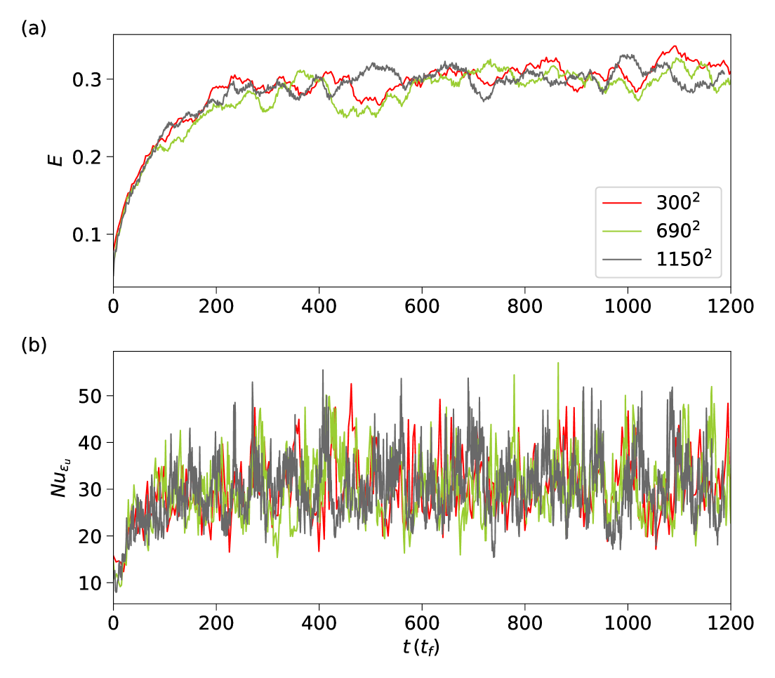
Figure 11: (a) Evolution of the domain-averaged energy $E(t)$ for $Pr=0.1,Ra=3\times 10^{8}$ using three different spatial resolutions. The similarity of the evolutions of $E$, in the statistical sense, suggests that the transient time and the mean energy in the steady state do not depend on the spatial resolution. (b) $Nu_{\varepsilon_{u}}$ exhibits strong fluctuations, especially at moments when a rapid decay is observed in $E(t)$.

To verify this, we performed simulations for a few governing parameters with different spatial resolutions and compared the temporal evolution of the integral quantities. In figure 11, we show the evolution of $E$ for $Pr=0.1,Ra=3\times 10^{8}$ in three different simulations, for mesh cells of $300^{2}$, $690^{2}$, and $1150^{2}$. We can see that the growth of $E$ in the initial stage (for $t<120\,t_{\mathrm{f}}$) is similar in all simulations, although the evolutions differ slightly for intermediate stages. However, once $E(t)$ stops growing and starts fluctuating about some mean, the average value of energy in the steady state does not depend on the spatial resolution. We find that the mean energy for $t>400t_{\mathrm{f}}$ in figure 11 differs only by at most 2%. We also show the evolution of $Nu_{\varepsilon_{u}}(t)$ in figure 11(b) for the three simulations and observe wild fluctuations, especially when $E(t)$ decreases rapidly over a short time interval. Thus, the flow properties in the steady state seem to be largely unaffected by the spatial resolution used in the transient state.

Figure 12: Evolution of the kinetic energy in the intermediate stage of the transient state for $Pr=1,Ra=10^{12}$. Computational time is close to one million core-hours for the simulation with $5210^{2}$ mesh cells—much bigger than one thousand core hours needed for simulation with $690^{2}$ cells. It is clear that performing high-$Ra$ simulation in the transient state with full resolution is infeasible.

Similarly, figure 12 shows $E(t)$ for intermediate stages of the transient state for $Pr=1,Ra=10^{12}$. We start the simulation with a coarse resolution having $690^{2}$ mesh cells (red curve). While $E(t)$ is still growing, we ramp up the resolution and start another simulation with $5210^{2}$ mesh cells (green curve), in addition to continuing the original one. Figure 12 shows that the trajectories of $E(t)$ in both simulations are similar, while the computational resources differ substantially. On the one hand, simulation with the coarse mesh consumes only one thousand core hours, and the segment shown in figure 12 was obtained in just eight hours on 128 cores. On the other hand, simulation with the finer mesh takes more than 900 hours on 1024 cores (green curve). As the transient time is nearly $8000\,t_{\mathrm{f}}$ for these parameters (see figure 4), one would need to run the simulation with $5210^{2}$ mesh cells for 72000 hours on 1024 cores to attain the steady state, which is clearly impossible at present.

In table 1 we list the important parameters of all the present simulations.

$Pr$	$Ra$	$N_{e}N^{2}$	$Nu$	$Re$	$t_{\mathrm{sim}}\,(t_{\mathrm{f}})$
0.1	$10^{6}$	$690^{2}$	5.91	1916	605
0.1	$2\times 10^{6}$	$300^{2}$	7.05	2747	1159
0.1	$3\times 10^{6}$	$690^{2}$	7.88	3396	461
0.1	$6\times 10^{6}$	$300^{2}$	10.04	4980	2684
0.1	$10^{7}$	$690^{2}$	11.77	6526	853
0.1	$2\times 10^{7}$	$500^{2}$	15.35	9497	1171
0.1	$3\times 10^{7}$	$690^{2}$	17.50	12065	1415
0.1	$10^{8}$	$1150^{2}$	23.43	22179	539
0.1	$3\times 10^{8}$	$1150^{2}$	31.30	43601	442
0.1	$10^{9}$	$2070^{2}$	42.54	95682	208
0.1	$3\times 10^{9}$	$2230^{2}$	59.15	200000	222
0.1	$10^{10}$	$3122^{2}$	84.70	446812	153
1	$3\times 10^{6}$	$300^{2}$	6.01	289	6375
1	$6\times 10^{6}$	$300^{2}$	7.11	423	6622
1	$8\times 10^{6}$	$300^{2}$	8.18	530	3630
1	$9\times 10^{6}$	$300^{2}$	8.64	580	5512
1	$10^{7}$	$690^{2}$	9.03	625	3246
1	$1.5\times 10^{7}$	$300^{2}$	13.3	918	7055
1	$2\times 10^{7}$	$690^{2}$	14.8	1108	1879
1	$3\times 10^{7}$	$690^{2}$	17.3	1376	2782
1	$6\times 10^{7}$	$690^{2}$	21.5	2010	2584
1	$10^{8}$	$690^{2}$	25.0	2665	1717
1	$3\times 10^{8}$	$690^{2}$	35.6	4936	2379
1	$6\times 10^{8}$	$690^{2}$	44.2	7385	1178
1	$10^{9}$	$700^{2}$	50.9	12012	2112
1	$3\times 10^{9}$	$1150^{2}$	67.1	20958	1479
1	$10^{10}$	$1150^{2}$	94.5	43533	989
1	$3\times 10^{10}$	$1610^{2}$	130.2	89031	1105
1	$10^{11}$	$2070^{2}$	184.4	197733	785
1	$3\times 10^{11}$	$3122^{2}$	264.0	393303	250
1	$10^{12}$	$5210^{2}$	394.2	1085094	253

Table 1: Important parameters of direct numerical simulations in a 2D box of $\Gamma=1$. We list the Prandtl number, the Rayleigh number, the total number of mesh cells in the entire flow domain $N_{e}N^{2}$, the Nusselt number, the Reynolds number, and the simulation time after the flow attains a steady state, $t_{\mathrm{sim}}$.

References

- Castaing et al. (1989) Castaing, B., Gunaratne, G., Kadanoff, L., Libchaber, A. & Heslot, F. 1989 Scaling of hard thermal turbulence in Rayleigh-Bénard convection. J. Fluid Mech. 204, 1–30.
- Chillà & Schumacher (2012) Chillà, F. & Schumacher, J. 2012 New perspectives in turbulent Rayleigh-Bénard convection. Eur. Phys. J. E 35, 58.
- Doering (2020) Doering, C. R. 2020 Absence of evidence for the ultimate state of turbulent Rayleigh-Bénard convection. Phys. Rev. Lett. 124, 229401.
- Doering et al. (2019) Doering, C. R., Toppaladoddi, S. & Wettlaufer, J. S. 2019 Absence of evidence for the ultimate regime in two-dimensional Rayleigh-Bénard convection. Phys. Rev. Lett. 123, 259401.
- Foroozani et al. (2014) Foroozani, N., Niemela, J. J., Armenio, V. & Sreenivasan, K. R. 2014 Influence of container shape on scaling of turbulent fluctuations in convection. Phys. Rev. E 90, 063003.
- Foroozani et al. (2017) Foroozani, N., Niemela, J. J., Armenio, V. & Sreenivasan, K. R. 2017 Reorientations of the large-scale flow in turbulent convection in a cube. Phys. Rev. E 95, 033107.
- Grossmann & Lohse (2000) Grossmann, S. & Lohse, D. 2000 Scaling in thermal convection: a unifying theory. J. Fluid Mech. 407, 27–56.
- Grossmann & Lohse (2001) Grossmann, S. & Lohse, D. 2001 Thermal convection for large Prandtl numbers. Phys. Rev. Lett. 86, 3316–3319.
- Howard (1972) Howard, L. N. 1972 Bounds on flow quantities. Annu. Rev. Fluid Mech. 4 (1), 473–494, arXiv: https://doi.org/10.1146/annurev.fl.04.010172.002353.
- Iyer et al. (2020) Iyer, K. P., Scheel, J. D., Schumacher, J. & Sreenivasan, K. R. 2020 Classical 1/3 scaling of convection holds up to Ra = . Proc. Natl. Acad. Sci. USA 117 (14), 7594–7598, arXiv: https://www.pnas.org/content/117/14/7594.full.pdf.
- Kadanoff (2001) Kadanoff, L. P. 2001 Turbulent heat flow: Structures and scaling. Phys. Today 54 (8), 34–39, arXiv: https://pubs.aip.org/physicstoday/article-pdf/54/8/34/16746047/34_1_online.pdf.
- Lam et al. (2002) Lam, S., Shang, X.-D., Zhou, S.-Q. & Xia, K.-Q. 2002 Prandtl number dependence of the viscous boundary layer and the Reynolds numbers in Rayleigh-Bénard convection. Phys. Rev. E 65, 066306.
- Lohse & Shishkina (2023) Lohse, D. & Shishkina, O. 2023 Ultimate turbulent thermal convection. Phys. Today 76 (11), 26–32, arXiv: https://pubs.aip.org/physicstoday/article-pdf/76/11/26/20085578/26_1_pt.3.5341.pdf.
- Lohse & Shishkina (2024) Lohse, D. & Shishkina, O. 2024 Ultimate Rayleigh–Bénard turbulence. Rev. Mod. Phys. 96, 035001.
- Niemela et al. (2000) Niemela, J. J., Skrbek, L., Sreenivasan, K. R. & Donnelly, R. J. 2000 Turbulent convection at very high Rayleigh numbers. Nature 404, 837–840.
- Pandey (2021) Pandey, A. 2021 Thermal boundary layer structure in low-Prandtl-number turbulent convection. J. Fluid Mech. 910, A13.
- Pandey et al. (2022a) Pandey, A., Krasnov, D., Schumacher, J., Samtaney, R. & Sreenivasan, K. R. 2022a Similarities between characteristics of convective turbulence in confined and extended domains. Physica D 442, 133537.
- Pandey et al. (2022b) Pandey, A., Krasnov, D., Sreenivasan, K. R. & Schumacher, J. 2022b Convective mesoscale turbulence at very low Prandtl numbers. J. Fluid Mech. 948, A23.
- Pandey et al. (2016) Pandey, A., Kumar, A., Chatterjee, A. G. & Verma, M. K. 2016 Dynamics of large-scale quantities in Rayleigh-Bénard convection. Phys. Rev. E 94, 053106.
- Pandey & Sreenivasan (2021) Pandey, A. & Sreenivasan, K. R. 2021 Convective heat transport in slender cells is close to that in wider cells at high Rayleigh and Prandtl numbers. Europhys. Lett. 135 (2), 24001.
- Pandey & Verma (2016) Pandey, A. & Verma, M. K. 2016 Scaling of large-scale quantities in Rayleigh-Bénard convection. Phys. Fluids 28 (9), 095105, arXiv: https://doi.org/10.1063/1.4962307.
- Pandey et al. (2016) Pandey, A., Verma, M. K., Chatterjee, A. G. & Dutta, B. 2016 Similarities between 2D and 3D convection for large Prandtl number. Pramana - J. Phys. 87, 13.
- Samuel & Verma (2024) Samuel, R. & Verma, M. K. 2024 Bolgiano-Obukhov scaling in two-dimensional Rayleigh-Bénard convection at extreme Rayleigh numbers. Phys. Rev. Fluids 9, 023502.
- Samuel et al. (2024) Samuel, R. J., Bode, M., Scheel, J. D., Sreenivasan, K. R. & Schumacher, J. 2024 No sustained mean velocity in the boundary region of plane thermal convection. J. Fluid Mech. 996, A49.
- Scheel et al. (2013) Scheel, J. D., Emran, M. S. & Schumacher, J. 2013 Resolving the fine-scale structure in turbulent Rayleigh-Bénard convection. New J. Phys. 15, 113063.
- Scheel et al. (2012) Scheel, J. D., Kim, E. & White, K. R. 2012 Thermal and viscous boundary layers in turbulent Rayleigh–Bénard convection. J. Fluid Mech. 711, 281–305.
- Scheel & Schumacher (2016) Scheel, J. D. & Schumacher, J. 2016 Global and local statistics in turbulent convection at low Prandtl numbers. J. Fluid Mech. 802, 147–173.
- Schmalzl et al. (2004) Schmalzl, J., Breuer, M. & Hansen, U. 2004 On the validity of two-dimensional numerical approaches to time-dependent thermal convection. Europhys. Lett. 67, 390–396.
- Schumacher et al. (2015) Schumacher, J., Götzfried, P. & Scheel, J. D. 2015 Enhanced enstrophy generation for turbulent convection in low-Prandtl-number fluids. Proc. Natl. Acad. Sci. USA 112, 9530–9535.
- Schumacher & Sreenivasan (2020) Schumacher, J. & Sreenivasan, K. R. 2020 Colloquium: Unusual dynamics of convection in the sun. Rev. Mod. Phys. 92, 041001.
- Shraiman & Siggia (1990) Shraiman, B. I. & Siggia, E. D. 1990 Heat transport in high-Rayleigh-number convection. Phys. Rev. A 42, 3650–3653.
- Siggia (1994) Siggia, E. D. 1994 High Rayleigh number convection. Annu. Rev. Fluid Mech. 26 (1), 137–168, arXiv: https://doi.org/10.1146/annurev.fl.26.010194.001033.
- Smith & Yakhot (1993) Smith, L. M. & Yakhot, V. 1993 Bose condensation and small-scale structure generation in a random force driven 2D turbulence. Phys. Rev. Lett. 71, 352–355.
- Sreenivasan et al. (2002) Sreenivasan, K. R., Bershadskii, A. & Niemela, J. J. 2002 Mean wind and its reversal in thermal convection. Phys. Rev. E 65, 056306.
- Stevens et al. (2011) Stevens, R., Lohse, D. & Verzicco, R. 2011 Prandtl and Rayleigh number dependence of heat transport in high Rayleigh number thermal convection. J. Fluid Mech. 688, 31–43.
- Stevens et al. (2010) Stevens, R., Verzicco, R. & Lohse, D. 2010 Radial boundary layer structure and Nusselt number in Rayleigh-Bénard convection. J. Fluid Mech. 643, 495–507.
- Stevens et al. (2024) Stevens, R. J., Hartmann, R., Verzicco, R. & Lohse, D. 2024 How wide must Rayleigh–Bénard cells be to prevent finite aspect ratio effects in turbulent flow? J. Fluid Mech. 1000, A58.
- Tiwari et al. (2025) Tiwari, H., Sharma, L. & Verma, M. K. 2025 Compressible turbulent convection at very high Rayleigh numbers. Int. J. Heat Mass Transfer 242, 126821.
- van der Poel et al. (2011) van der Poel, E. P., Stevens, R. J. A. M. & Lohse, D. 2011 Connecting flow structures and heat flux in turbulent Rayleigh-Bénard convection. Phys. Rev. E 84, 045303(R).
- van der Poel et al. (2013) van der Poel, E. P., Stevens, R. J. A. M. & Lohse, D. 2013 Comparison between two- and three-dimensional Rayleigh-Bénard convection. J. Fluid Mech. 736, 177–194.
- Verma (2018) Verma, M. K. 2018 Physics of Buoyant Flows. Singapore: World Scientific, arXiv: https://www.worldscientific.com/doi/pdf/10.1142/10928.
- Verma et al. (2017) Verma, M. K., Kumar, A. & Pandey, A. 2017 Phenomenology of buoyancy-driven turbulence: recent results. New J. Phys. 19 (2), 025012.
- Verzicco & Camussi (1999) Verzicco, R. & Camussi, R. 1999 Prandtl number effects in convective turbulence. J. Fluid Mech. 383, 55–73.
- Weiss & Ahlers (2011) Weiss, S. & Ahlers, G. 2011 Turbulent Rayleigh–Bénard convection in a cylindrical container with aspect ratio = 0.50 and Prandtl number Pr = 4.38. J. Fluid Mech. 676, 5–40.
- Xi & Xia (2008) Xi, H. & Xia, K. 2008 Flow mode transitions in turbulent thermal convection. Phys. Fluids 20, 5104.
- Xia et al. (2003) Xia, K. Q., Sun, C. & Zhou, S. Q. 2003 Particle image velocimetry measurement of the velocity field in turbulent thermal convection. Phys. Rev. E 68, 066303.
- Zhang et al. (2017) Zhang, Y., Zhou, Q. & Sun, C. 2017 Statistics of kinetic and thermal energy dissipation rates in two-dimensional turbulent Rayleigh-Bénard convection. J. Fluid Mech. 814, 165–184.
- Zhu et al. (2018) Zhu, X., Mathai, V., Stevens, R. J. A. M., Verzicco, R. & Lohse, D. 2018 Transition to the ultimate regime in two-dimensional Rayleigh-Bénard convection. Phys. Rev. Lett. 120, 144502.