Enceladus’s Limit Cycle

Abstract

Enceladus exhibits some remarkable phenomena, including water geysers spraying through surface cracks, a global ice shell that is librating atop an ocean, a large luminosity, and rapid outward orbital migration. Here we model the coupled evolution of Enceladus’s orbit and interior structure. We find that Enceladus is driven into a periodic state—a limit cycle. Enceladus’s observed phenomena emerge from the model, and the predicted values for the orbital eccentricity, libration amplitude, shell thickness, and luminosity agree with observations. A single limit cycle lasts around ten million years, and has three distinct stages: (1) freezing, (2) melting, and (3) resonant libration. Enceladus is currently in the freezing stage, meaning that its ice shell is getting thicker. That pressurizes the ocean, which in turn cracks the shell and pushes water up through the cracks. In this stage the orbital eccentricity increases, as Saturn pushes Enceladus deeper into resonance with Dione. Once the eccentricity is sufficiently high, tidal heating begins to melt the shell, which is the second stage of the cycle. In the third stage the shell remains close to 3km thick. At that thickness the shell’s natural libration frequency is resonant with the orbital frequency. The shell’s librations are consequently driven to large amplitude, for millions of years. Most of the tidal heating of Enceladus occurs during this stage, and the observed luminosity is a relic from the last episode of resonant libration.

1 Introduction

Enceladus is a small moon of Saturn, with a radius of 252km. It is covered by an ice shell, which conceals a global ocean below (Thomas et al., 2016). Near the south pole, water vapor and frozen mist spray from the ocean through four long and deep parallel fractures in the shell (Porco et al., 2006), in the form of $\sim 100$ geysers (Porco et al., 2014). These observations, and many others, were gathered by the Cassini mission, from 2005-2017. The wealth of Enceladus’s observed phenomema provides valuable clues into how tides operate, both in Enceladus and in Saturn. See, e.g., Nimmo et al. (2023) and Ćuk et al. (2024) for reviews.

Enceladus’s ocean is prevented from freezing over by tidal heating within Enceladus, which is driven by the eccentricity of its orbit around Saturn. The current eccentricity is

$$e_{\rm obs} = 0.0047\ .$$ (1)

Tidal heating should quickly circularize the orbit. But circularization is prevented by tides on Saturn, which push Enceladus deeper into its 2:1 mean motion resonance (MMR) with its outer partner, Dione, thereby maintaining a resonantly forced eccentricity for Enceladus.

The leading mechanism for tidal pushing by Saturn used to be equilibrium tides. In the equilibrium tide scenario, Enceladus raises a tidal bulge in Saturn, and the time-varying bulge is presumed to dissipate energy, at a rate parameterized by an unknown tidal quality factor in Saturn ($Q_{S}$). But recent observations found that Saturn’s moons are migrating outward at rates that are inconsistent with this scenario (Lainey et al., 2012, 2020). Lainey et al find that the migration timescale is

$$\tau_{\rm obs}\sim 10{\rm Gyr}\ ,$$ (2)

for six of the moons, including Enceladus. In contrast, the equilibrium tide scenario predicts a migration timescale that increases rapidly with distance from Saturn, and so should be extremely long for the far-out moons, especially Rhea and Titan. Rhea’s well-observed migration rate is particularly constraining, and would imply $Q_{S}\approx 300$ under equilibrium tides. That $Q_{S}$ is not only extremely small for a fluid body such as Saturn, but is also inconsistent with the values of $Q_{S}$ implied by other moons. Fuller et al. (2016) showed that the fast observed migration rates could be understood if the moons were being pushed out by the “resonance locking” mechanism, rather than equilibrium tides. In resonance locking, a moon excites a near-resonant oscillation mode of Saturn. Dissipation of the mode’s energy forces the moon to maintain an orbital frequency slightly less than the mode’s frequency. As Saturn evolves, the mode’s frequency is presumed to decrease, on Gyr timescales. That forces the moon’s frequency to decrease too, implying outward migration. We adopt the resonance locking mechanism in this paper.

Observations of the rotation state of Enceladus’s surface find that it is librating on the timescale of its orbit. Its forced libration amplitude is found to be

$$\gamma_{\rm obs}\approx 0.1^{\circ}$$ (3)

with $\sim 20\%$ error bars (Thomas et al., 2016; Park et al., 2024). This libration is forced by Saturn, as Saturn traces out its epicycle as seen from Enceladus. But $\gamma_{\rm obs}$ is too large for an entirely solid moon. Instead, there must be a thin ice shell that is librating on top of a global ocean. From $\gamma_{\rm obs}$, the inferred average thickness of the shell is

$$d_{\rm obs}\sim 20{\rm-}30\ {\rm km}\ ,$$ (4)

(Thomas et al., 2016; Cadek et al., 2016; Park et al., 2024). Measurements of Enceladus’s quadrupolar gravity (Iess et al., 2014) and shape (Park et al., 2024) provide similar values for the shell thickness, while the ocean below is inferred to have a depth comparable to $d_{\rm obs}$. Beneath the ocean lies a rocky core, with radius $\sim 200$km. The ocean is known to be in contact with the core, as deduced from the fact that particulates in the water jets are salty (Hsu et al., 2015).

The ice shell thickness $d_{\rm obs}$ has at least two major consequences. First, the librations of the shell distort its shape, which causes frictional heating; the rate of energy dissipation is inversely proportional to $d_{\rm obs}$ (see eq. 26 below). Second, heat is conducted outward through the shell. Since the temperature jump across the shell is known, as is the conductivity of ice, knowing the value of $d_{\rm obs}$ allows a determination of the moon’s cooling rate. It is found that the cooling rate is

$$C_{\rm obs}\sim 20{\rm-}30\ {\rm GW}\ ,$$ (5)

where 80% of this number comes from global conduction through an ice shell with thickness $d_{\rm obs}$. The additional $20\%$ is inferred from localized heat flow in the south pole region (Le Gall et al., 2017; Nimmo et al., 2023; Park et al., 2024).

The cooling rate of equation (5) is an important clue. Meyer & Wisdom (2007) show that Enceladus’s heating rate should be 1.1GW, under the assumptions that the Enceladus-Dione MMR is in equilibrium, and that $Q_{S}=18,000$ (in the equilibrium tide scenario). But the fast migration timescale found by Lainey et al. (2020) implies a much greater heating rate, that exceeds even equation (5) by a factor of $\sim$4 (see eq. 25 below). Although there are large uncertainties in the inferred heating rate, if heating does not balance cooling it would mean that the assumption that the MMR is in equilibrium is incorrect.

2 Overview of the Limit Cycle

In this paper we evolve Enceladus under a minimal model that includes the physical processes described above: resonance locking with a mode in Saturn; the 2:1 MMR between Enceladus and Dione; heat dissipation that comes from tidal distortions of the ice shell; conduction through the shell; and freezing and melting of the shell. We find that Enceladus naturally settles into a limit cycle, without artificial tweaking of parameters.

Before embarking on the equations and their solution, we provide here an overview of the limit cycle.

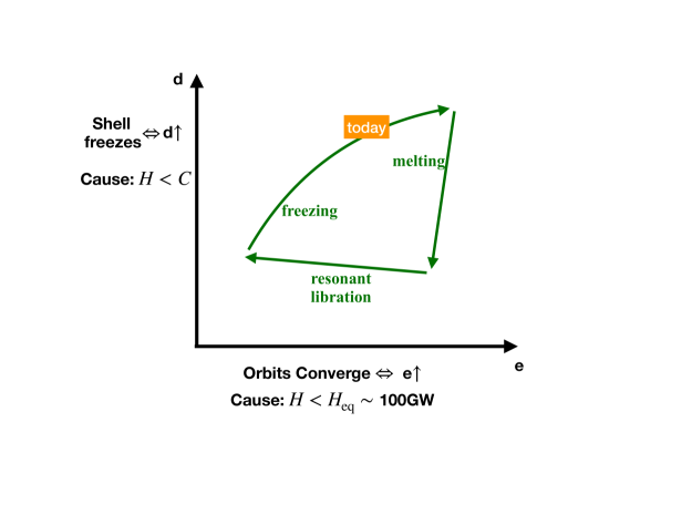
Figure 1: Cartoon View of the Limit Cycle: The axes are Enceladus’s orbital eccentricity ($e$), and the thickness of its ice shell ($d$) .

Figure 1 displays a cartoon version in the $e$-$d$ plane. (See Fig. 3 for the non-cartoon version.) The $e$ axis also acts as a surrogate for the distance between Enceladus and Dione: $e$ rises when the moons converge, and falls when they diverge, due to the 2:1 MMR. The trajectory of the limit cycle is primarily driven by two energy rates: Enceladus’s heating rate and its cooling rate ($H$ and $C$). Heating is caused by tidal distortions of the ice shell, and we assume that the heat is deposited near the base of the shell, where the ice is soft and slushy. Cooling is due to conduction through the shell, and so $C\propto 1/d$. We describe the three stages in turn, starting at the freezing stage, which is where Enceladus finds itself today:

1. Freezing: $d$ is increasing because $H<C$. To understand why $e$ also increases in the freezing stage, we turn to the orbital dynamics, which set a critical heating rate at which the Dione-Enceladus MMR remains in equilibrium, $H_{\rm eq}\sim 100$GW (eqs. 18 & 25). If $H>H_{\rm eq}$, the moons’ orbits are driven to diverge; otherwise, they are driven to converge. The dynamics are similar to those of an accretion disk, where loss of orbital energy leads to spreading of the disk. Here, if there is sufficient loss of orbital energy, i.e., if $H$ is large enough, then the moons also diverge. In the freezing stage there is little heating. In particular, $H<H_{\rm eq}$, which drives the orbits to converge, and $e$ increases. The reason freezing ends is that $H\propto e^{2}$ (ignoring the $d$ dependence for now), because the heating is driven by Enceladus’s epicyclic motion. As $e$ rises, $H$ increases, until eventually $H>C$, at which point freezing transitions to melting.

2. Melting. Melting is a runaway process (Peale & Cassen, 1978), during which $d$ decreases by an order of magnitude, while $e$ remains nearly constant. Towards the beginning of this stage, $H\propto e^{2}/d$ (see eq. 26 for the full expression), while $C\propto 1/d$. Therefore after melting begins ($H>C$), the decrease of $d$ cannot tip the balance in favor of cooling. Instead, the heating rate increases, which causes more rapid melting, which causes $H$ to increase more, leading to runaway. As $d$ continues to decrease, it approaches the critical thickness for libration resonance, $d_{\rm res}\sim 3$km (eq. 29), and $H$ increases enormously. Shortly after $d$ sweeps through $d_{\rm res}$, $H$ falls sufficiently that cooling finally becomes competitive with heating.

3. Resonant Libration. This is perhaps the most surprising stage. The thickness of the shell remains slightly below $d_{\rm res}$ for millions of years, as heating and cooling nearly balance each other, with $H\sim C\sim 200$GW. The heating rate is so large because the shell’s forced libration amplitude becomes very big near resonance, which produces large distortions. Almost all of Enceladus’s heating occurs during this stage. The present-day cooling luminosity (eq. 5) is a modest remnant of that epoch. An important additional consequence of the large heating is that $H>H_{\rm eq}$. Therefore Enceladus and Dione are pushed apart, and $e$ drops. This allows a new cycle of freezing to begin, with very small $e$ and hence very small heating.

3 Equations of Motion

3.1 Orbital Equations

Enceladus and Dione are observed to be in a 2:1 mean motion resonance (MMR). Dione is the outer moon, and lies slightly exterior to the nominal location of the MMR. Saturn is pushing Enceladus outwards, deeper into resonance with Dione. We model Enceladus’s and Dione’s long-term orbital evolution by evolving their angular momenta and energies via

$$\dot{L}+\dot{L}_{2} = T$$ (6)

$$\dot{E}+\dot{E}_{2} = nT-H\ .$$ (7)

Unsubscripted quantities refer to Enceladus, and ones with subscript 2 refer to Dione; $L$, $L_{2}$, $E$, and $E_{2}$ are the angular momenta and energies of the moons, which we express as functions of their mean motions ($n$ and $n_{2}$) and eccentricities ($e$ and $e_{2}$), i.e., for Enceladus

$$L = m(GM_{S})^{2/3}n^{-1/3}\left(1-{e^{2}\over 2}\right)$$ (8)

$$E = -m(GM_{S})^{2/3}{1\over 2}n^{2/3}\ ,$$ (9)

where $M_{S}$ is Saturn’s mass and $m$ is Enceladus’s. The analogous equations apply to Dione’s $L_{2}$ and $E_{2}$, in terms of $m_{2}$, $n_{2}$, and $e_{2}$.

The quantities on the right-hand sides of equations (6)–(7) are the torque on Enceladus by Saturn ($T$), which also changes Enceladus’s orbital energy at the rate $nT$ by conservation of Jacobi constant; and $H$, which is the tidal heating rate within Enceladus. Expressions for $T$ and $H$ are provided below. Although there are four unknowns ($n$, $n_{2}$, $e$, and $e_{2}$) and only two equations, we turn the equations into a closed set by making two further assumptions: that Dione’s orbit is circular, and that Enceladus’s eccentricity takes on its resonantly forced value due to the 2:1 MMR

$$e = 0.76{m_{2}\over M_{S}}{n\over n-2n_{2}}\ .$$ (10)

We note that the MMR between Enceladus and Dione has resonant argument $\phi=2\lambda_{2}-\lambda-{\varpi}$, and affects Enceladus’s eccentricity, but not Dione’s. Dione’s current eccentricity is very small (0.0022), and so setting it to zero is an adequate approximation.

With this setup one may integrate equations (6)–(7) numerically for $n$ and ${n}_{2}$, once $T$ and $H$ are known.

3.2 Torque and Reduced Orbital Equations

We model the torque $T$ within the framework of the resonance locking mechanism (Fuller et al., 2016). We assume that there is a mode in Saturn that has natural frequency $\omega$ in the inertial frame, and that $\omega$ decreases on timescale $\tau$, i.e.,

$${\dot{\omega}\over\omega}=-{1\over\tau}\$$ (11)

where $\tau$ is determined solely by the evolution of Saturn, and is very long ($\gtrsim$Gyr). Because the mode’s amplitude $A$ is forced by Enceladus it is inversely proportional to the frequency mismatch: $A\propto 1/\Delta$, where

$$\Delta = {\omega-n\over\omega}\ ,$$ (12)

which is assumed to satisfy $0<\Delta\ll 1$. The mode loses energy in Saturn’s rotating frame at a rate $\propto A^{2}$, which causes the moon’s orbit to gain energy at a rate $\dot{E}\propto A^{2}$ and, by conservation of Jacobi constant, to gain angular momentum at the rate $T=\dot{E}/n$. Consequently, we write $T$ in equations (6)–(7) as

$$T={{\rm const.}\over\Delta^{2}}\ ,$$ (13)

The differential equations (6)–(7) are time-dependent, via their dependence on $T(\omega(t))$. But provided $\omega$ decays sufficiently slowly, one may remove that dependence by changing variables from $n$ to $\Delta$, which is the fractional distance of $n$ to its “nominal” value of $\omega$. In a similar vein, we change from $n_{2}$ to

$$\Delta_{2} = {\omega-2n_{2}\over\omega}\ ,$$ (14)

which is the fractional distance of Dione’s inner 2:1 MMR from its nominal value of $\omega$. Thus $\Delta$ and $\Delta_{2}$ will be our surrogates for the semimajor axes of the two moons, relative to the corotation radius of the resonance locking mode. The nominal MMR is at $\Delta=\Delta_{2}$, and we will always have $\Delta<\Delta_{2}$, i.e., Dione is exterior to nominal MMR.

As we show in Appendix A, the resulting equations for $\Delta$ and $\Delta_{2}$, under the assumption that $\Delta\ll 1$ and $\Delta_{2}\ll 1$, are

$${\epsilon}\dot{\Delta}+\dot{\Delta}_{2}-3\epsilon e\dot{e} = \left({\Delta_{\rm eq}^{2}\over\Delta^{2}}-1\right){1+\epsilon\over\tau}$$ (15)

$$\dot{\Delta}_{2}-6\epsilon e\dot{e} = \left({H\over H_{\rm eq}}-1\right){1\over\tau}\ ,$$ (16)

where

$$\epsilon\equiv{m\over 2^{1/3}m_{2}}$$ (17)

is the ratio of the moons’ nominal angular momenta, $\Delta_{\rm eq}$ is a constant that replaces the unknown constant in equation (13), and

$$H_{\rm eq} = {m_{2}\left(GM_{S}n\right)^{2/3}\over 3\cdot 2^{2/3}\tau}$$ (18)

is the equilibrium heating rate, with the symbol $n$ now considered to be constant. Equations (15)–(16) are to be supplemented with

$$e=0.76{m_{2}\over M_{S}}{1\over\Delta_{2}-\Delta}\ ,$$ (19)

and an expression for $H$ (provided below), whereupon they form a closed set of differential equations for $\Delta$ and $\Delta_{2}$, without explicit time-dependence.

When evaluating expressions, we set

$$m = 1.08\times 10^{23}{\rm g}$$ (20)

$$m_{2} = 1.095\times 10^{24}{\rm g}$$ (21)

$$M_{S} = 5.683\times 10^{29}{\rm g}$$ (22)

$$n = 2\pi/(1.3702{\rm day})$$ (23)

whence

$$\epsilon = 0.078$$ (24)

$$H_{\rm eq} = 116{\rm GW}\left({10{\rm Gyr}\over\tau}\right)$$ (25)

3.3 Tidal Heating

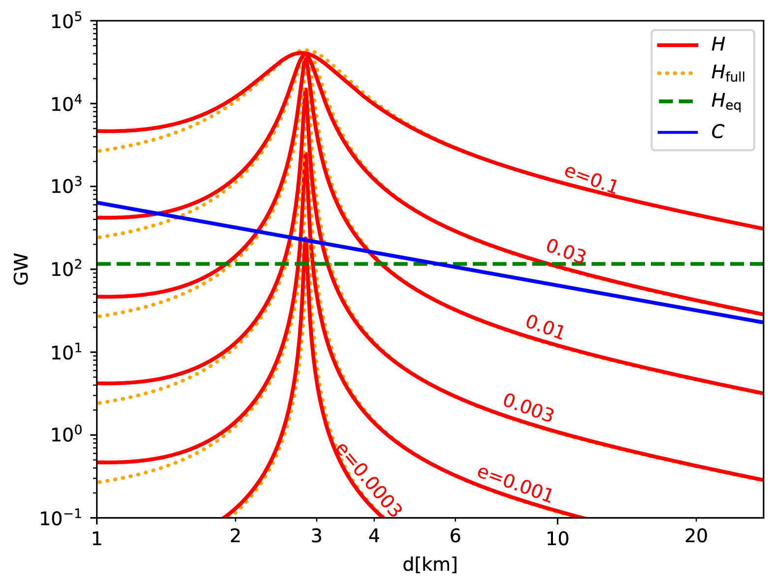
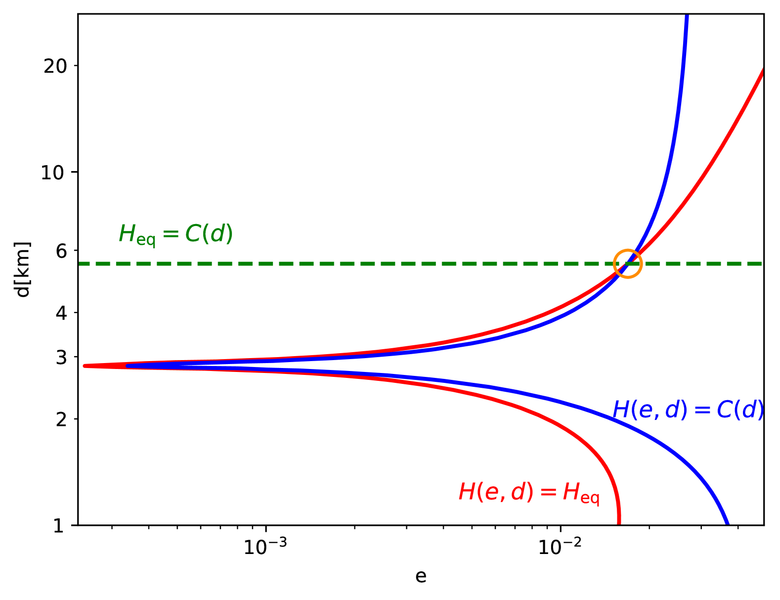
Figure 2: Heating and Cooling Rates. Left panel: The red curves are the tidal heating rate, $H(e,d)$, at selected values of $e$, setting ${Q_{\rm ice}}=25$. The orange dotted curves ($H_{\rm full}$) are for a more general heating model that does not assume that the shell is very rigid. But since $H_{\rm full}$ leads to little change over the range of $d$’s of interest, we use $H$ in this paper for simplicity. The green horizontal dashed line is the heating rate for equilibrium pushing (eq. 18, at our fiducial value of $\tau=10$Gyr). And blue is the cooling due to conduction through the shell (eq. 30). Right panel: Equilibrium curves in the $e$-$d$ plane, produced by equating rates in the left panel. The red curve represents equilibrium of the MMR, and the blue curve is where the ice shell thickness does not change. The circle is the global (unstable) equilibrium point.

Tidal heating within Enceladus ($H$) is assumed to be due to deformations of its ice shell. We model Enceladus as being composed of a rigid solid core covered by an ocean, which in turn is covered by a thin ice shell. The undistorted core and shell are taken to be spherically symmetric. If Enceladus were on a circular orbit it would be in a spin-synchronous state, and the shell’s shape would be determined by the lowest energy response to Saturn’s tidal field. In that case, there would be no energy dissipation. But because $e\neq 0$, time-dependent forcing from Saturn distorts the shell, which dissipates energy. We calculate the time averaged elastic energy within the ice shell, $\langle E_{\rm elas}\rangle$, that is induced by the epicyclic motion of Saturn, as seen from Enceladus. We then set the heating rate to $H={2n\over{Q_{\rm ice}}}\langle E_{\rm elas}\rangle$, where ${Q_{\rm ice}}$ is the quality factor for the elastic flexure of the shell, and is set to a constant value. See the companion paper Lithwick (2025) for the full calculation. That calculation is similar to Van Hoolst et al. (2013) in physical content, but yields an analytic expression for the heating rate. In Figure 2 (left panel), we plot the resulting heating rate $H$ vs. shell thickness ($d$), for various values of $e$, as solid red curves. The heating spikes at $d_{\rm res}=2.8$km are due to a libration resonance. In particular, when the shell’s thickness is equal to $d_{\rm res}$, the frequency of the shell’s free librations is equal to the orbital frequency. That resonance drives the shell to a large forced libration amplitude, which is the cause for the enhanced heating. The enhanced heating at the libration resonance will play an important role in the limit cycle behavior.

The analytic expression for the heating curves in the figure is as follows (Lithwick 2025):

$$H(e,d) = {21\pi\over 5}{\rho_{w}^{2}R^{8}n^{5}\over\mu{Q_{\rm ice}}}{e^{2}\over d}\times$$ (26)

$$\left({3\over 7}+{4\over 7}{1\over\left({\omega_{\rm lib}^{2}/n^{2}}-1\right)^{2}+\left({Q_{\rm ice}}{\cal R}\right)^{-2}+4e^{2}}\right)\ \ \ \ \$$

where $R=252$km is Enceladus’s radius; $\rho_{w}=0.93$gm/cm³ is the density of water, which we take here to be the same as that of ice; $\mu=4$ GPa is the rigidity of ice; and the Poisson ratio of ice has been set to $1/3$. The first term in brackets (3/7) is from the radial tide, and the second is from the librational tide (Murray & Dermott, 1999). The resonant denominator in the librational tide depends primarily on the frequency of free librations of the ice shell,

$${\omega_{\rm lib}^{2}\over n^{2}} = {d_{\rm res}\over d}$$ (27)

where

$$d_{\rm res} = {9\over 10}R{n^{2}R\over g}h_{*}$$ (28)

$$= 2.8{\rm km},$$ (29)

$g=Gm/R^{2}$, and the dimensionless number $h_{*}\approx 2$, which incorporates the effect of a rigid core (Lithwick 2025). Finally, the “hardness parameter” is ${\cal R}\approx d$/(0.84 km) for Enceladus.

In general, the hardness parameter can play an important role (Goldreich & Mitchell, 2010). But for Enceladus ${\cal R}\gtrsim 1$ throughout the evolution. Physically, the limit ${\cal R}\gg 1$ corresponds to the shell being very rigid, which means that it hardly changes its shape as it undergoes its forced librations. In writing equation (26), we have therefore chosen to simplify it, for clarity, by taking the limit ${\cal R}\gg 1$. That is why ${\cal R}$ only plays a modest role in that equation. But we show in the figure what happens for arbitrary values of ${\cal R}$, as orange dotted curves ($H_{\rm full}$). The match between solid and dotted curves is adequate for $d\gtrsim 1.5$km. Hence we adopt the above simplified expression for $H$ for the remainder of this paper.

3.4 Freezing and Melting

The thickness of the ice shell, $d$, affects the evolution via its effect on $H(e,d)$. And $d$ is in turn affected by tidal heating, which can melt the ice. To model the evolution of $d$, we assume that most of the heating is deposited near the base of the ice shell, because the slushy mixture there is much more dissipative than the solidly frozen ice higher up. The rate at which energy leaves the moon (the cooling rate) is

$$C(d) = k_{\rm ice}{\Delta T\over d}4\pi R^{2}$$ (30)

where $k_{\rm ice}=4\times 10^{5}$erg/cm/K is the conductivity of the shell, which is approximated to be constant, and $\Delta T=200$K is the temperature jump across the shell. We set the net heating equal to the rate of energy change due to freezing/melting i.e.,

$$H(e,d)-C(d)=-4\pi R^{2}\rho_{w}\left(\ell+c_{p}{\Delta T\over 2}\right)\dot{d}$$ (31)

where $\ell=3.34\times 10^{9}$erg/g is the latent heat of fusion, and $c_{p}=10^{7}$erg/g/K is the heat capacity of ice. Note that the second term in brackets is due to the change in internal energy, as melting of ice necessitates that the remaining ice warms up. Equation (31) is our final evolutionary equation; it gives $\dot{d}$ as a function of the variables $e$ and $d$. In the absence of heating ($H(e,d)\rightarrow 0$), our adopted parameters imply a freezing timescale $d/\dot{d}=6.4$Myr $\times\left(d/(20{\rm km})\right)^{2}$.

Equation (30) is shown in the left panel of Figure 2 for our fiducial parameters. As described in §2, the limit cycle is largely controlled by the relative values of $H$, $C$, and $H_{\rm eq}$. Therefore in the right panel of Figure 2, we display the three resulting equilibrium curves in the $e$-$d$ plane.

3.5 Summary of Equations, Choice of Parameters, and Global Equilibrium

The equations of motion for $\Delta$ and $\Delta_{2}$, which encode the locations of the two moons, are given by equations (15)–(16), supplemented with equations (17)–(19). For the heating rate $H$, we use equation (26). The equilibrium of equations (15)–(16) has both moons migrating in lockstep with the frequency of the driving mode within Saturn. Zeroing the time derivatives in those equations gives the equilibrium state:

$$\Delta = \Delta_{\rm eq}$$ (32)

$$H(e,d) = H_{\rm eq}\ ,$$ (33)

where the latter is the red curve in the right panel of Figure 2. The third and final equation of motion is for $d$. It is given by equation (31), for which $H(e,d)$ is also needed. Its equilibrium occurs when

$$H(e,d) = C(d)\ ,$$ (34)

which is the blue curve in the right panel of Figure 2.

For the bulk of this paper, we choose the following values for the three uncertain parameters in our model:

$$\tau = 10\ {\rm Gyr}$$ (35)

$${Q_{\rm ice}} = 25$$ (36)

$$\Delta_{\rm eq} = 0.02$$ (37)

The value of $\tau$ is comparable to the one inferred by Lainey et al. (2020). For ${Q_{\rm ice}}$, we expect it to be much larger than unity, because most of the ice shell is solidly frozen. And although the value of $\Delta_{\rm eq}$ is very uncertain, we find it does not play a significant role. Towards the end of the paper we show what happens when these parameters are varied.

We conclude this subsection by solving for the global equilibrium, $H=C=H_{\rm eq}$, which will be used as the initial condition of the integration. The equilibrium thickness of the ice shell follows from equating ${\cal H}_{\rm eq}=C(d)$, which gives $d_{\rm eq}=5.50$ km. This value is proportional to $\tau$, but is uninfluenced by other uncertain parameters. To obtain the equilibrium $e$, we insert $d_{\rm eq}$ into equation (33), from which we obtain numerically $e_{\rm eq}=0.017$. One then finds via equation (19) that $\Delta_{2,\rm eq}=\Delta_{\rm eq}+8.7\times 10^{-5}$.

3.6 Numerical Integration

In order to integrate the equations of motion, we use equation (19) to replace $e\dot{e}\rightarrow-{e^{2}\over\Delta_{2}-\Delta}(\dot{\Delta}_{2}-\dot{\Delta})$ in equations (15)–(16), and at each timestep we solve the latter two equations algebraically for $\dot{\Delta}$ and $\dot{\Delta}_{2}$. We then integrate those time-derivatives, along with equation (31) for $\dot{d}$.

4 Evolution

4.1 From Unstable Equilibrium to Limit Cycle

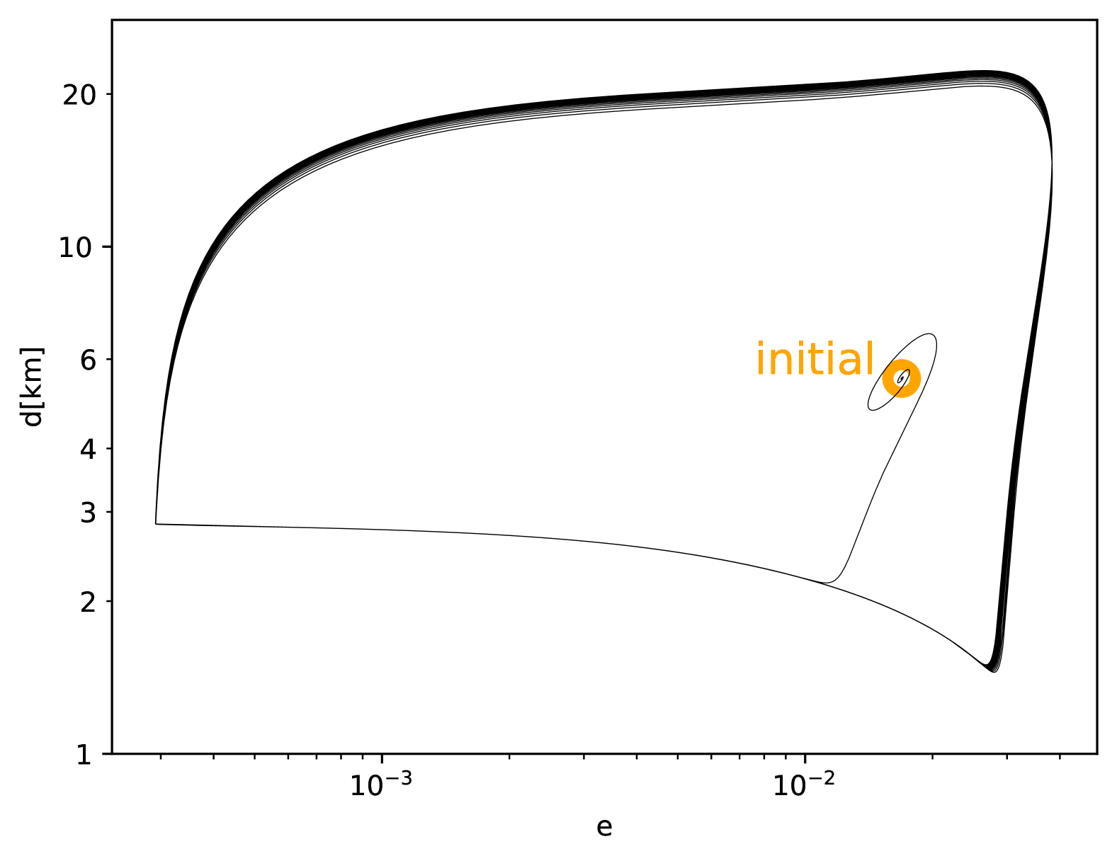
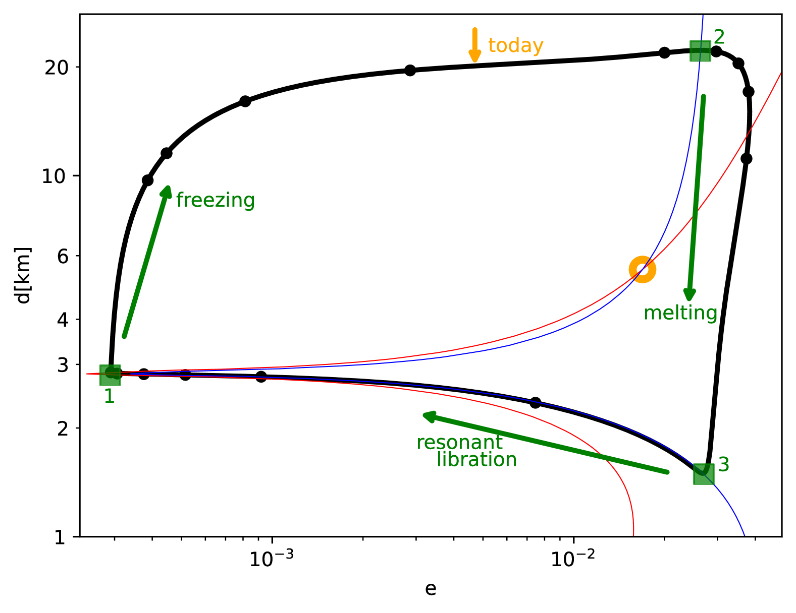
Figure 3: Numerical Evolution in the $e$-$d$ Plane. Left panel: The black curve displays the system’s evolution, after it is initialized at the global equilibrium point. It escapes from equilibrium, and then traces out repeating limit cycles. Right panel: The black curve is the same as in the left panel, but restricted to the limit cycle. The black circles on the curve are separated by 1 Myr, over the course of one cycle. The blue and red curves are the equilibrium heating and cooling curves, repeated from Figure 2, with the blue showing $H=C$, and the red showing $H=H_{\rm eq}$. .

We initialize the integration at the global equilibrium point presented at the end of §3.5. In the $e$-$d$ plane, the system spirals away from its initial state, and converges to a repeating limit cycle, as shown in the left panel of Figure 3. Each cycle lasts 13.3 Myr. The right panel shows the steady cycle, with the freezing, melting, and resonant libration stages marked out:

• Freezing (1 $\rightarrow$ 2): The shell thickens from $2.8$km to $22$km, while Enceladus’s eccentricity rises because it is being pushed deeper into its MMR with Dione. Enceladus is currently in this phase. The vertical orange arrow marks where $e=e_{\rm obs}=0.0047$.

• Melting (2 $\rightarrow$ 3): The shell melts from $22$km to $1.5$km, while Enceladus’s eccentricity remains high, at $e\sim 0.04$.

• Resonant Libration (3 $\rightarrow$ 1): the shell’s thickness slowly grows towards $d_{\rm res}=2.8$ km, the thickness for exact resonant libration (eq. 29). Most of the heating occurs during this phase, and one consequence of the extreme heating is that Enceladus is driven away from Dione’s MMR, lowering its resonantly forced eccentricity to 0.0003.

The black circles in this panel are separated by 1 Myr. Also shown are the equilibrium curves for heating and cooling, repeated from the right panel of Figure 2. At point 2, melting begins when the $H=C$ curve is crossed. The subsequent melting phase is seen to be a runaway process: while millions of years are required to melt the shell thickness by a factor of $\sim 2$, the shell then melts to 1.5km in under a million years. Immediately before Enceladus crosses point 3, its cooling rate grows to around $10C_{\rm obs}$, because $C\propto 1/d$. Even more dramatically, the heating rate spikes to $\sim 1000C_{\rm obs}$, because $d\sim d_{\rm res}$. Immediately after point 3 heating is very high, albeit much less than in the aforementioned spike. That forces $e$ to drop very quickly to $\sim 0.005$, by pushing the moons apart. Subsequently, the evolution in the resonant libration stage slows down, as the boost in heating caused by $d\sim d_{\rm res}$ is counterbalanced by the decrease in heating due to a very small $e$. Millions of years elapse at the end of the resonant libration stage, before the system re-enters its current freezing phase.

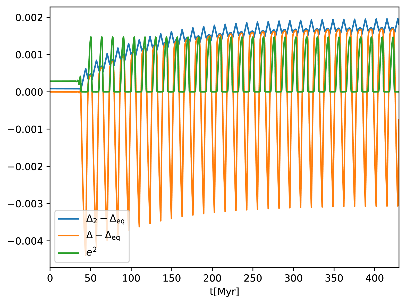
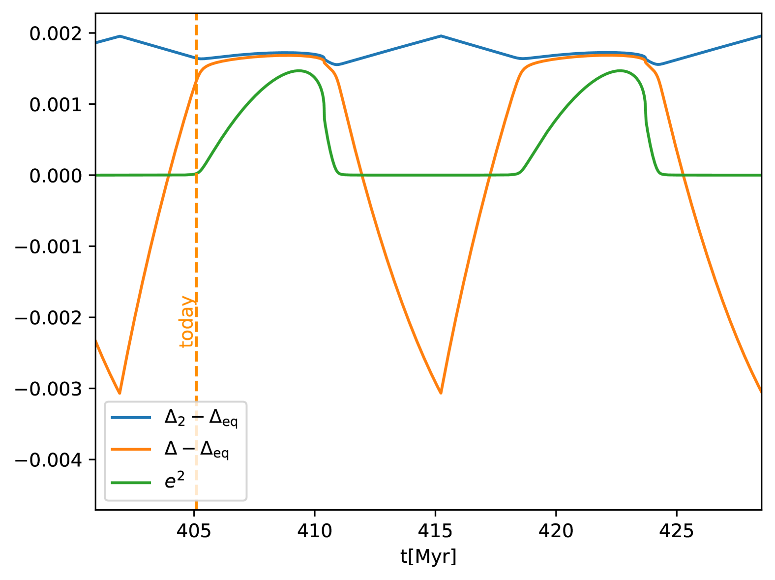
Figure 4: Evolution of $\Delta$, $\Delta_{2}$, and $e^{2}$, where we have subtracted the constant $\Delta_{\rm eq}=0.02$ from the $\Delta$’s. Left panel: Initial evolution. Right panel: Evolution in the limit cycle. The vertical line marked “today” shows when $e=e_{\rm obs}=0.0047$.

Figure 4 highlights the role of Dione’s MMR in the evolution by showing $\Delta$ and $\Delta_{2}$ at early times (left panel) and in the steady limit cycle (right panel). Recall that $\Delta$ is the fractional distance, in frequency-space, of Enceladus from its nominal position $\omega$, and $\Delta_{2}$ is the fractional distance of Dione’s MMR from $\omega$ (eqs. 12&14). From the left panel, we see that it takes over 100Myr for the moons’ positions to reach their final limit cycle.

4.2 Behavior in the Limit Cycle

In the right panel of Figure 4, the first minimum of the orange curve at 402Myr corresponds to the beginning of the freezing stage (point 1 in right panel of Fig. 3). Following that time, the orange curve increases, indicating outward motion of Enceladus, and the blue curve decreases, indicating inward motion of Dione. The moons continue to converge until $e^{2}$ (green curve) hits its maximum, at 409Myr. Note that $e$ is inversely proportional to $\Delta_{2}-\Delta$, and so it tracks convergence/divergence. In the limit cycle plot (right panel of Fig. 3), the maximum $e$ occurs when the red $H=H_{\rm eq}$ curve is crossed, because convergence is driven by $H<H_{\rm eq}$, and ends when $H=H_{\rm eq}$.

The moons converge from 402 to 409Myr. But there is a qualitative transition at $\sim$405Myr. Before that time, there is rapid convergence of the moons’ $\Delta$’s, or equivalently of their semimajor axes, while $e$ remains very low. But the subsequent convergence is much slower, as the moons are already very close to exact resonance, and further convergence drives the rise of $e$. Those two types of behavior are evident from the equation of motion (eq. 16); each type corresponds to one of the two terms on the left-hand side dominating the other. After 409Myr, the moons’ orbits diverge, until the next cycle begins. Virtually all of the divergence occurs during the resonant libration stage.

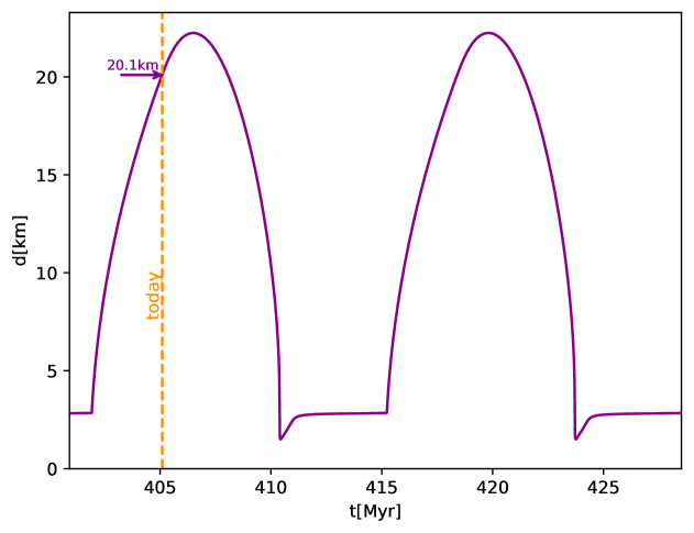
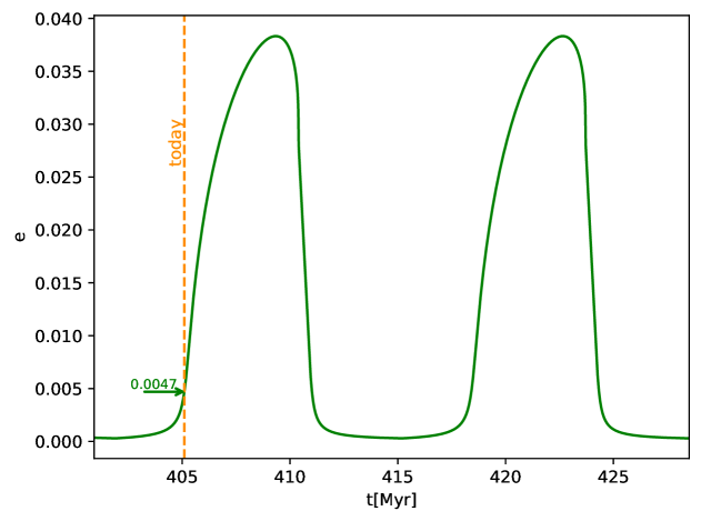
Figure 5: Evolution of $d$ and $e$ over two limit cycles.

Figure 5 shows the temporal evolution of $d$ and $e$ over the course of two limit cycles. The vertical line (“today”) is when $e=e_{\rm obs}=0.0047$ and $d$ is growing. Of course, that happens once per cycle, but we arbitrarily choose to focus on the cycle beginning at 402Myr. At the current time, $e$ has just commenced rapid growth, while $d$ is already close to its maximum value. The shell thickness is currently 20.1km in the model, which is comparable to $d_{\rm obs}$ (eq. 4). In the resonant libration stage, most of the time is spent with $d$ and $e$ fairly constant, before that stage ends at $415$Myr. The enormous heating and cooling that occur at the start of this stage are not very apparent in this figure. They are associated with the small rise in $d$ immediately after 410.4Myr, and the concurrent extremely rapid decline in $e$.

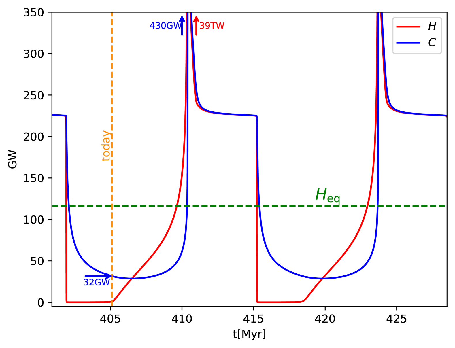
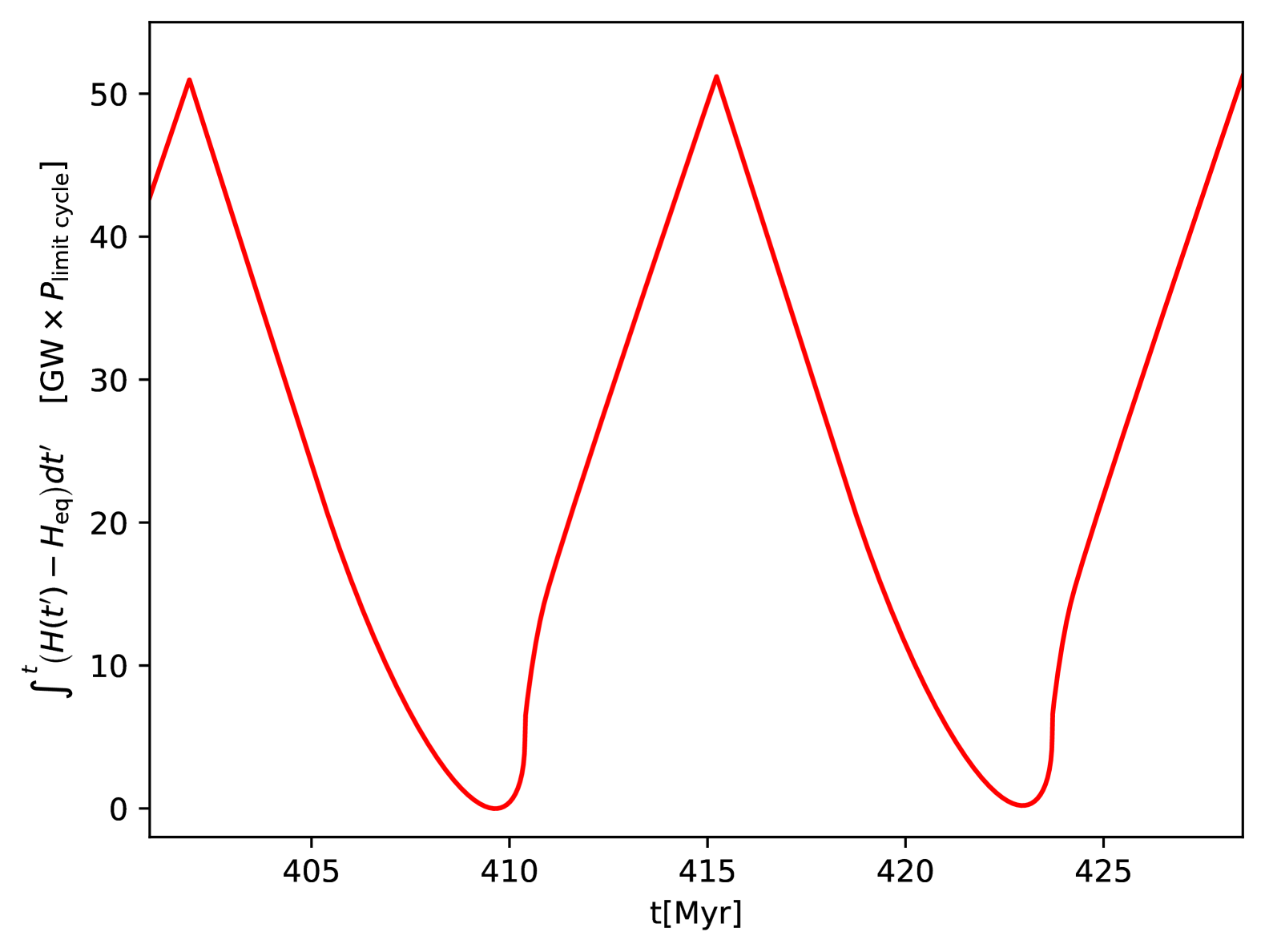
Figure 6: Top panel: Heating and Cooling Rates. Bottom panel: Integrated heating rate.

Figure 6 (top panel) shows the heating and cooling rates, which drive most of the system’s behavior. At the current time the cooling rate is $C=32$GW, consistent with the observationally inferred $C_{\rm obs}$ (eq. 5). The heating rate is much smaller than that, $H=1$ GW. The current value of $H$ is so small primarily because $e$ is small. But the two moons are presently converging, and $e$ is about to rise dramatically (right panel of Fig. 4). Thus, after 405Myr, $H\propto e^{2}$ also rises dramatically, until $H$ crosses $C$. The time when $H=C$, which occurs at 406.5Myr, marks the beginning of the melting stage. In the limit cycle plot (Fig. 3), that time is labelled 2, which is when the blue curve is crossed. Returning to the top panel of Figure 6, we see that $H$ continues to rise past $C$, until it reaches $H=H_{\rm eq}$ at 409Myr. As noted previously, that marks the time that the moons stop converging, and begin to diverge. Divergence lowers $e$ and reduces $H$; but the timescale for that to happen is relatively long. Instead, runaway melting occurs first: with $H>C$, and both of those rates nearly inversely proportional to $d$, the shell melts at the rate $\dot{d}\approx-{\rm const}/d$ (eq. 31). If that equation continued to apply, the shell would melt to $d=0$ in a finite time. In actuality, the shell does initially get thinner at an increasingly rapid rate (Fig. 5, top panel). But before it hits $d=0$, it crosses the critical value for resonant libration, $d=2.8$km, when the heating rate becomes enormous: $H=39$TW, as seen from the heating curves of Figure 2 (left panel). As $d$ continues to decrease beyond the point where $\omega_{\rm lib}=n$, the librational tide acquires a dependence on $d$ (eq. 26), which allows cooling to finally catch up with heating, thereby preventing the shell from melting entirely. The shell melts to a thickness of 1.5km, whereupon the resonant libration stage commences, at 410.4Myr. In the limit cycle plot (Fig. 3), that occurs at point 3, where the blue $H=C$ curve is crossed again. The enormous spike in $H$ immediately before the end of the melting stage affects the energy budget. But because it lasts a short time, the net effect is modest. From the bottom panel of Figure 6, which shows the integrated heating rate, the spike immediately before 410.4Myr injects an extra energy of 6.5GW$\times P_{\rm limit\ cycle}$ (on top of what would be injected if $H=H_{\rm eq}$), where $P_{\rm limit\ cycle}=13.3$Myr is the period of a limit cycle. In comparison, the subsequent resonant libration stage injects an extra energy of 44.8GW$\times P_{\rm limit\ cycle}$. Thus the resonant libration stage is primarily responsible for heating Enceladus. That conclusion is also apparent from the limit cycle plot (Fig. 3), which shows that most of the drop in $e$—which is driven by $H-H_{\rm eq}$—occurs during resonant libration.

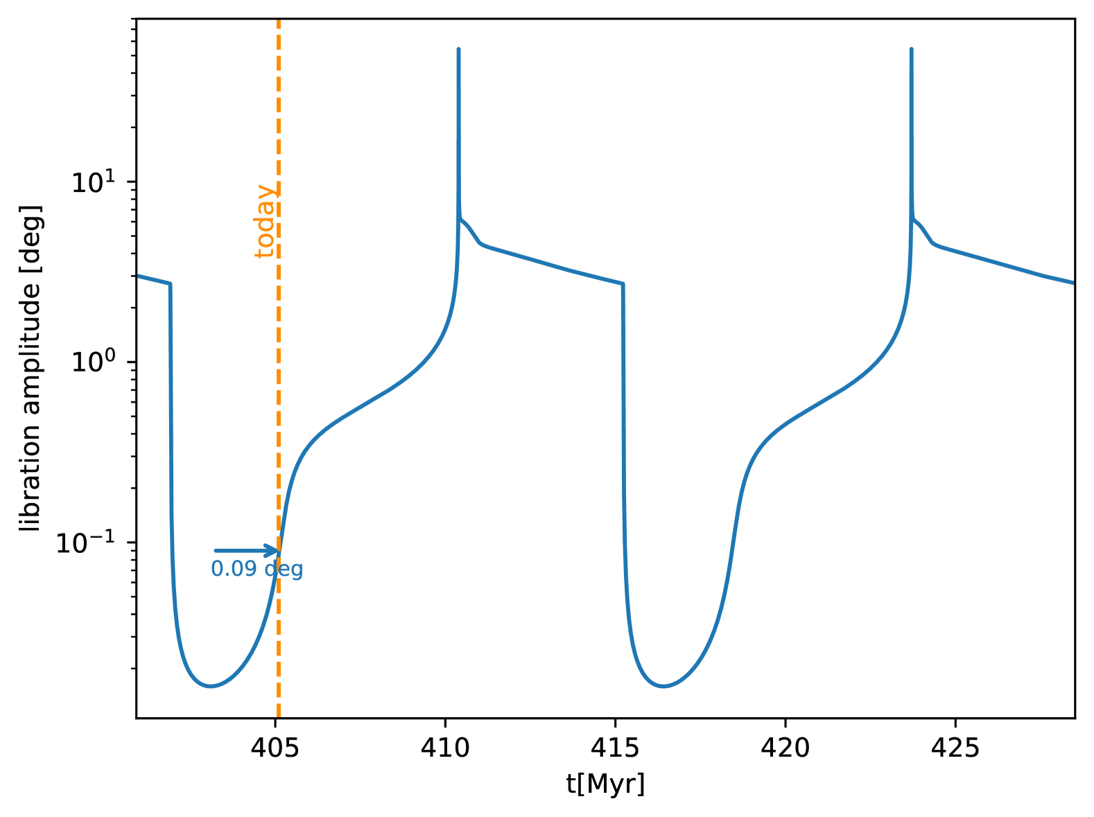
Figure 7: Libration Amplitude

Figure 7 shows the shell’s libration amplitude $\hat{\gamma}_{\rm ice}$, which is approximately given by

$$\hat{\gamma}_{\rm ice}\approx 2e{\omega_{\rm lib}^{2}\over|\omega_{\rm lib}^{2}-n^{2}|}$$ (38)

(See Lithwick 2025 for the full expression that is plotted in the figure.) At the current time, $\hat{\gamma}_{\rm ice}=0.09^{\circ}$, in agreement with the observed $\gamma_{\rm obs}$ (eq. 3). And during the extreme spike in heating at the end of the melting stage, $\hat{\gamma}_{\rm ice}$ reaches as high as $50^{\circ}$, i.e., the shell rotates nearly a full revolution each orbital period. Of course, it is that large libration amplitude that drives the large heating rate.

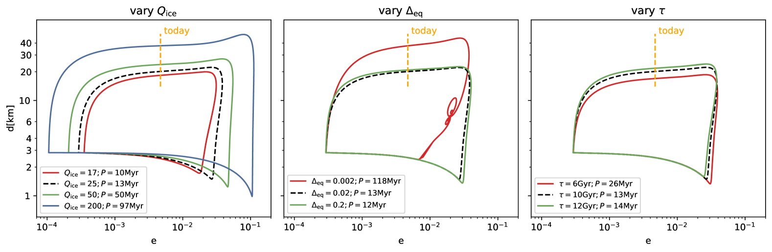
Figure 8: Limit Cycle for Different Parameters. In each of the three panels, we vary one parameter, while keeping the other parameters at their fiducial values. The insets show the values of the parameter that is varied, as well as the period of the limit cycle for that parameter value.

In the resonant libration stage, $d$ slowly grows towards its resonant value $d_{\rm res}=2.8$km, while the heating remains high: $H\sim 230$GW throughout most of this stage. This behavior may be understood by examining the $H$ and $C$ curves in the left panel of Figure 2. As the system follows the $C$ curve towards $d_{\rm res}$, which has magnitude $C(d=d_{\rm res})=230$GW, heating very nearly balances cooling. If $e$ were to be held artificially fixed, then the system would remain in thermal equilibrium, with $H=C$, and a little to the left of the resonant peak at $d_{\rm res}$. This is a stable equilibrium: an increase in $d$ enhances heating relative to cooling, which melts the shell, decreasing $d$. In contrast, the equilibrium just to the right of the resonant peak is unstable. Now, with $e$ allowed to evolve, the fact that the heating rate of $\sim 230$GW exceeds $H_{\rm eq}$ forces the moons to diverge, lowering the resonantly forced $e$, which lowers the red curve in Figure 2. Eventually, the red curve can no longer reach the blue curve, which occurs when $e=e_{\rm min}=0.0003$. When that happens, the resonant libration stage ends. Heating cannot compete with cooling, causing $d$ to increase beyond $d_{\rm res}$. That makes heating extremely small because it can no longer take advantage of the resonant peak. The system thus re-enters the freezing stage. At the beginning of the freezing stage, with $H\approx 0$, the cooling rate shrinks from 230GW in inverse proportion to the growing $d$ (Fig. 6), crossing through 32GW today. The fact that the heating is very small forces the moons to converge, and the cycle repeats.

5 Discussion

We presented a simple model for the thermal and tidal dynamics of Enceladus. With our chosen values for the three uncertain parameters in the model (${Q_{\rm ice}}$, $\Delta_{\rm eq}$, and $\tau$), we found that Enceladus does not remain at its equilibrium point, but instead follows a limit cycle in the $e$-$d$ plane. We consider most uncertain input physics in the model to be the resonant locking hypothesis, as modelled by equation (13) for Saturn’s torque on Enceladus.

Many of Enceladus’s observed properties are consistent with it currently being in the freezing phase of its limit cycle, including $e_{\rm obs}$, $\gamma_{\rm obs}$, $d_{\rm obs}$, and $C_{\rm obs}$. As hinted at the end of the previous section, the reason Enceladus escapes from equilibrium is that the equilibrium is thermally unstable (Shao & Nimmo, 2022). In the left panel of Figure 2, global equilibrium occurs where the blue and green curves intersect. At that position, the red curves fall more steeply than the blue, implying that an increase in $d$ favors cooling over heating, which increases $d$ even more. Previous studies have considered limit cycles for Io (Ojakangas & Stevenson, 1986) and Enceladus (Meyer & Wisdom, 2008; Shoji et al., 2014), but driven by a different mechanism, in which the moon’s dissipative properties were modelled in a more ad hoc way.

A difficulty with our model is that Enceladus’s current migration rate appears to be too fast. In the right panel of Figure 4, the slope of the orange curve at the time marked “today” yields that $\dot{n}/n\approx-10/\tau=-1/{\rm Gyr}$, which is around ten times faster than that of Lainey et al. (2020). Whether this is truly a discrepancy is not certain, as Lainey et al’s value relies on modelling of the tides on both Saturn and on Enceladus, in a different way than we do, and is complicated by the interaction between Enceladus and Dione. But if there is a discrepancy, our model might be adjusted in a number of ways to resolve it: for example, by including a more elaborate model for Saturn’s tidal torque, or by including tidal damping of Dione. In Figure 4, one sees that Enceladus’s migration rate slows very soon after “today.” A horizontal line in that plot corresponds to a migration time of $\tau=10$Gyr. Hence the migration rate becomes close to Lainey et al’s value in the very near future. It is therefore possible that a modest adjustment of our model would suffice to resolve the difficulty.

We find that the behavior of the limit cycle is not greatly sensitive to the values of the parameters. In Figure 8 we show how the limit cycle changes when ${Q_{\rm ice}}$, $\Delta_{\rm eq}$, and $\tau$ are varied. From the left panel we see that as ${Q_{\rm ice}}$ is varied from 17 to 200, the present-day thickness of the ice shell increases from $18$km to 37km; the minimum shell thickness decreases from 1.7km to 1km; and the period of a cycle increases from 10 to 97 Myr. We also find that for ${Q_{\rm ice}}\lesssim 16$, the limit cycle goes away, and Enceladus reaches its global equilibrium. From the middle panel, we see that one may vary $\Delta_{\rm eq}$ by two orders of magnitude, without much effect on the cycle. In the right panel, we vary $\tau$ by a factor of 2, and also find not much of an effect on the cycle. However, if either $\tau\lesssim 5$Gyr, or $\tau\gtrsim 13$Gyr, Enceladus does not evolve away from its initial state, i.e., the global equilibrium state is stable. The reason for this sensitivity may be understood from the left panel of Figure 2: changing $\tau$ moves the $H_{\rm eq}$ line up and down. If it is moved too far up, the global equilibrium is to the left of the resonant peak, and hence is stable. And if it is moved too far down, the global equilibrium occurs where the red and blue curves are nearly parallel to each other, indicating neutral stability. Nonetheless, by adjusting the initial value of $d$, we have found that limit cycles persist for $\tau$ up to 18Gyr. We leave a more thorough investigation of parameter space to the future.

In conclusion, we have shown that Enceladus is likely not in equilibrium. Instead, its semimajor axis, eccentricity, and shell thickness, are tracing out a limit cycle. In addition to the evidence presented above, three further lines of evidence support this conclusion:

1. The expression for the heating rate (eq. 26) shows that $H\approx(25/{Q_{\rm ice}})$GW today, after inserting the observed $d_{\rm obs}$ and $e_{\rm obs}$. Thus one would require an unreasonably low ${Q_{\rm ice}}$ for the heating to be comparable to $C_{\rm obs}\sim 20$-$30$GW. Shao & Nimmo (2022) have argued similarly. This strongly suggests that heating is less that $C_{\rm obs}$, implying that Enceladus is currently in the freezing stage, in which its ice shell is thickening.

2. The cracks seen in the south pole region are a natural consequence of a thickening ice shell (e.g., Rudolph et al., 2022). As the shell thickens, the increased volume occupied by ice relative to water overpressurizes the ocean, and the resulting stresses are sufficiently strong to crack Enceladus’s ice shell. By contrast, tidal stresses are likely too weak to crack the shell, as they are an order of magnitude weaker.

3. The shapes of craters on Enceladus are more relaxed than they should be based on present conditions. But the shapes have been explained by a past episode of extreme heating, in which the heat flux exceeded 150 mW m^-2, or 120GW averaged over the moon (Bland et al., 2012). Such a high heat flux occurs in our model throughout the resonant libration stage, when $C\approx 230$GW.

One might wonder whether Europa exhibits behavior similar to Enceladus. An important difference between the two moons is that Europa’s ice shell cannot experience resonant libration, whatever its thickness (Goldreich & Mitchell, 2010, Lithwick 2025). As a result, Europa cannot experience a limit cycle of the type described in this paper.

Appendix A Derivation of Simplified Orbital Equations

We derive equations (15)–(16), starting from equations (6)–(9), together with our model for the resonance locking torque (eqs. 11–13). We first define the nominal angular momenta of the two moons as

$$L_{\rm nom} = m(GM_{S})^{2/3}\omega^{-1/3}$$ (A1)

$$L_{2,\rm nom} = m_{2}(GM_{S})^{2/3}(\omega/2)^{-1/3}$$ (A2)

We expand the angular momenta and energies to first order in $\Delta$, $\Delta_{2}$ (as defined in eq. 12 & 14) and in $e^{2}$:

$$L \approx L_{\rm nom}\left(1+{1\over 3}{\Delta}-{e^{2}\over 2}\right)$$ (A3)

$$L_{2} \approx L_{2,\rm nom}\left(1+{1\over 3}\Delta_{2}\right)$$ (A4)

$$E \approx \omega L_{\rm nom}\left(-{1\over 2}+{1\over 3}{\Delta}\right)$$ (A5)

$$E_{2} \approx {\omega\over 2}L_{2,\rm nom}\left(-{1\over 2}+{1\over 3}\Delta_{2}\right)$$ (A6)

We then write the torque equation (eq. 6) as follows:

$$T-\dot{L}_{\rm nom}-\dot{L}_{2,\rm nom} = {d\over dt}\left(L-L_{\rm nom}+L_{2}-L_{2,\rm nom}\right)$$ (A7)

which from equations (A3)–(A6) and equation (11) approximates to

$$T-{1\over 3\tau}\left(L_{\rm nom}+L_{2,\rm nom}\right)\approx\left(L_{\rm nom}+L_{2,\rm nom}\right){1\over 1+\epsilon}\left(\epsilon({1\over 3}\dot{\Delta}-e\dot{e})+{1\over 3}\dot{\Delta}_{2}\right)$$ (A8)

after defining

$$\epsilon \equiv {L_{\rm nom}\over L_{2,\rm nom}}={m\over 2^{1/3}m_{2}}$$ (A9)

We have assumed that the timescale of variation of our new variables ($\Delta$, $\Delta_{2}$, and $e$) is much shorter than $\tau$ in equation (11), which enables us to drop, e.g., $\dot{L}_{\rm nom}\Delta$ in comparison with $L_{\rm nom}\dot{\Delta}$.

For the power equation (eq. 7), we proceed similarly. But we first subtract $\omega\times$ (eq. 6), which gives

$$H = \omega\dot{L}+\omega\dot{L}_{2}-\dot{E}-\dot{E}_{2}$$ (A10)

after dropping the small term $(n-\omega)T$. Inserting the approximate forms for $L$ and $E$, and moving the time-derivative of the nominal pieces of those approximate forms to the left-hand-side of the equation, yields

$$H-{\omega\over 3\tau}\left(L_{\rm nom}+L_{2,\rm nom}\right)+{\omega\over 3\tau}L_{\rm nom}+{\omega\over 2\cdot 3\tau}L_{2,\rm nom}=-\omega L_{\rm nom}e\dot{e}+\omega L_{2,\rm nom}{1\over 6}\dot{\Delta}_{2}$$ (A11)

and then after multiplying through:

$${H(1+\epsilon)\over\omega\left(L_{\rm nom}+L_{2,\rm nom}\right)}-{1\over 6\tau}=-\epsilon e\dot{e}+{1\over 6}\dot{\Delta}_{2}$$ (A12)

Equations (A8) and (A12) are the equations that we integrate numerically in the body of the paper. The terms in these equations have transparent physical meanings. For example, the term on the right-hand-side of equation (A8) that is proportional to $\epsilon$ is the rate of change of Enceladus’s orbital angular momentum minus what it would have been on its nominal orbital expansion. And the other term is the same for Dione.

Finally, it is convenient to rewrite those two equations by introducing two new constants:

$$\Delta_{\rm eq} \equiv \left({3\tau T\Delta^{2}\over L_{\rm nom}+L_{2,\rm nom}}\right)^{1/2}$$ (A13)

$$H_{\rm eq} \equiv {\omega\over 6\tau(1+\epsilon)}\left(L_{\rm nom}+L_{2,\rm nom}\right)$$ (A14)

where the first expression is constant because $T\Delta^{2}=$ is constant (eq. 13). Equations (A8) and (A12) then turn into the equations given in the body of the paper (eqs. 15–16).

References

- Bland et al. (2012) Bland, M. T., Singer, K. N., McKinnon, W. B., & Schenk, P. M. 2012, Geophys. Res. Lett., 39, L17204, doi: 10.1029/2012GL052736
- Cadek et al. (2016) Cadek, O., Tobie, G., Van Hoolst, T., et al. 2016, Geophys. Res. Lett., 43, 5653, doi: 10.1002/2016GL068634
- Ćuk et al. (2024) Ćuk, M., El Moutamid, M., Lari, G., et al. 2024, Space Sci. Rev., 220, 20, doi: 10.1007/s11214-024-01049-2
- Fuller et al. (2016) Fuller, J., Luan, J., & Quataert, E. 2016, MNRAS, 458, 3867, doi: 10.1093/mnras/stw609
- Goldreich & Mitchell (2010) Goldreich, P. M., & Mitchell, J. L. 2010, Icarus, 209, 631, doi: 10.1016/j.icarus.2010.04.013
- Hsu et al. (2015) Hsu, H.-W., Postberg, F., Sekine, Y., et al. 2015, Nature, 519, 207, doi: 10.1038/nature14262
- Iess et al. (2014) Iess, L., Stevenson, D. J., Parisi, M., et al. 2014, Science, 344, 78, doi: 10.1126/science.1250551
- Lainey et al. (2012) Lainey, V., Karatekin, Ö., Desmars, J., et al. 2012, ApJ, 752, 14, doi: 10.1088/0004-637X/752/1/14
- Lainey et al. (2020) Lainey, V., Casajus, L. G., Fuller, J., et al. 2020, Nature Astronomy, 4, 1053, doi: 10.1038/s41550-020-1120-5
- Le Gall et al. (2017) Le Gall, A., Leyrat, C., Janssen, M. A., et al. 2017, Nature Astronomy, 1, 0063, doi: 10.1038/s41550-017-0063
- Meyer & Wisdom (2007) Meyer, J., & Wisdom, J. 2007, Icarus, 188, 535, doi: 10.1016/j.icarus.2007.03.001
- Meyer & Wisdom (2008) —. 2008, Icarus, 198, 178, doi: 10.1016/j.icarus.2008.06.012
- Murray & Dermott (1999) Murray, C. D., & Dermott, S. F. 1999, Solar System Dynamics, doi: 10.1017/CBO9781139174817
- Nimmo et al. (2023) Nimmo, F., Neveu, M., & Howett, C. 2023, Space Sci. Rev., 219, 57, doi: 10.1007/s11214-023-01007-4
- Ojakangas & Stevenson (1986) Ojakangas, G. W., & Stevenson, D. J. 1986, Icarus, 66, 341, doi: 10.1016/0019-1035(86)90163-6
- Park et al. (2024) Park, R. S., Mastrodemos, N., Jacobson, R. A., et al. 2024, Journal of Geophysical Research (Planets), 129, e2023JE008054, doi: 10.1029/2023JE008054
- Peale & Cassen (1978) Peale, S. J., & Cassen, P. 1978, Icarus, 36, 245, doi: 10.1016/0019-1035(78)90109-4
- Porco et al. (2014) Porco, C., DiNino, D., & Nimmo, F. 2014, AJ, 148, 45, doi: 10.1088/0004-6256/148/3/45
- Porco et al. (2006) Porco, C. C., Helfenstein, P., Thomas, P. C., et al. 2006, Science, 311, 1393, doi: 10.1126/science.1123013
- Rudolph et al. (2022) Rudolph, M. L., Manga, M., Walker, M., & Rhoden, A. R. 2022, Geophys. Res. Lett., 49, e2021GL094421, doi: 10.1029/2021GL094421
- Shao & Nimmo (2022) Shao, W. D., & Nimmo, F. 2022, Icarus, 373, 114769, doi: 10.1016/j.icarus.2021.114769
- Shoji et al. (2014) Shoji, D., Hussmann, H., Sohl, F., & Kurita, K. 2014, Icarus, 235, 75, doi: 10.1016/j.icarus.2014.03.006
- Thomas et al. (2016) Thomas, P. C., Tajeddine, R., Tiscareno, M. S., et al. 2016, Icarus, 264, 37, doi: 10.1016/j.icarus.2015.08.037
- Van Hoolst et al. (2013) Van Hoolst, T., Baland, R.-M., & Trinh, A. 2013, Icarus, 226, 299, doi: 10.1016/j.icarus.2013.05.036