Enhanced quantum frequency estimation by nonlinear scrambling

Abstract

Frequency estimation, a cornerstone of basic and applied sciences, has been significantly enhanced by quantum sensing strategies. Despite breakthroughs in quantum-enhanced frequency estimation, key challenges remain: static probes limit flexibility, and the interplay between resource efficiency, sensing precision, and potential enhancements from nonlinear probes remains not fully understood. In this work, we show that dynamically encoding an unknown frequency in a nonlinear quantum electromagnetic field can significantly improve frequency estimation. To provide a fair comparison of resources, we define the energy cost as the figure of merit for our sensing strategy. We further show that specific higher-order nonlinear processes lead to nonlinear-enhanced frequency estimation. This enhancement results from quantum scrambling, where local quantum information spreads across a larger portion of the Hilbert space. We quantify this effect using the Wigner-Yanase skew information, which measures the degree of noncommutativity in the Hamiltonian structure. Our work sheds light on the connection between Wigner-Yanase skew information and quantum sensing, providing a direct method to optimize nonlinear quantum probes.

Introduction.— Accurate frequency estimation plays a central role in various fields such as quantum communication Gisin and Thew (2007); Chen (2021), quantum sensing Degen et al. (2017); Pirandola et al. (2018); Montenegro et al. (2024), and quantum computation Aharonov (1999). Its importance extends to key applications in metrology Giovannetti et al. (2004, 2006, 2011); Udem et al. (2002); Descamps et al. (2023); Kuenstner et al. (2024); Boss et al. (2017); Cai et al. (2021), spectroscopy Roos et al. (2006); Schmitt et al. (2021); Lamperti et al. (2020), and precision timekeeping Ludlow et al. (2015). Quantum sensors, probes that exploit quantum phenomena, have been demonstrated to surpass the precision limits achievable by classical sensors in frequency estimation Haase et al. (2018); Bollinger et al. (1996); Degen et al. (2017); Montenegro et al. (2024); Giovannetti et al. (2004, 2006, 2011). Thus, the task of quantum frequency estimation has been pursued in various scenarios, including the use of decoherence-free subspaces for trapped particles in optical lattices Dorner (2012), continuous monitoring of qubit probes in noisy environments Albarelli et al. (2018, 2020), techniques involving adaptive coherent control Naghiloo et al. (2017); Rodríguez-García et al. (2024), and general scenarios in noisy metrology Huelga et al. (1997); Smirne et al. (2016); Haase et al. (2016); Macieszczak et al. (2014); Macieszczak (2015). Although quantum-enhanced sensing strategies have demonstrated remarkable precision in frequency estimation Donohue et al. (2018); Fröwis et al. (2014), several key questions remain. In particular, static methods based on the preparation of a given state do not allow for effective encoding, as only the eigenvalues of the free Hamiltonian depend on the frequency, while the eigenstates are entirely independent of it. This limits the achievable precision. We therefore ask: (i) Is it possible to remove this restriction using dynamical approaches, thereby increasing the flexibility of the quantum probe? (ii) Can a proper sensing resource be defined to quantify enhancements in frequency estimation? (iii) Is it possible to link the enhancement in frequency estimation to the internal Hamiltonian structure?

In this Letter, we address all the above issues. Regarding the first question, we encode the unknown frequency into the dynamical state of a quantized electromagnetic field with a nonlinear Hamiltonian. Once the frequency (unknown parameter) is dynamically encoded into a quantum state, we quantify the frequency precision limits using quantum estimation theory Helstrom (1969); Paris (2009). To address the second question, we define an energy cost figure of merit that quantifies enhancements in frequency estimation while balancing resource efficiency and estimation precision Liuzzo-Scorpo et al. (2018); Rodríguez-García et al. (2024). To address the third question, we examine our quantum sensing strategy in the broader context of quantum scrambling Garcia et al. (2023), which describes how local quantum information disperses across the degrees of freedom in a quantum system Zanardi (2001); Zhou and Luitz (2017); Khemani et al. (2018); Chen and Zhou (2018); Zhou and Swingle (2023); Aleiner et al. (2016); Harrow et al. (2021); Nahum et al. (2018); von Keyserlingk et al. (2018); Touil and Deffner (2024, 2020); Kobrin et al. (2024). In contrast to prior quantum sensing studies that focus on dominant scrambling quantifiers Li et al. (2023), we use the Wigner-Yanase skew information Wigner and Yanase (1963); Luo (2003); Chen (2005); Chen and Lian (2023); Luo and Zhang (2019), which enables us to quantify the degree of noncommutativity in the internal structure of the Hamiltonian Takagi (2019); Luo et al. (2012). In particular, we show that higher-order nonlinearities enhance frequency sensitivity, with maximal sensitivity closely aligning with the maximum value of the Wigner-Yanase skew information. This observation highlights the connection between quantum scrambling, measured using the Wigner-Yanase skew information Luo (2003), and the sensitivity of the probe to small changes in the unknown parameter.

Quantum metrological tools.— The uncertainty in estimating an unknown parameter $\omega$ encoded in a quantum state $\rho(\omega)$ obeys the quantum Cramér-Rao theorem Cramér (1999); Rao (1992); Helstrom (1967); Paris (2009):

$$\mathrm{Var}[\tilde{\omega}]\geq[M\mathcal{F}(\omega)]^{-1}\geq[MQ(\omega)]^{-1},$$ (1)

where $\mathrm{Var}[\tilde{\omega}]$ is the variance of a local unbiased estimator $\tilde{\omega}$ of the parameter $\omega$, $M$ is the number of measurement trials, $\mathcal{F}(\omega)$ is the classical Fisher information (CFI) with respect to the unknown parameter $\omega$, and $Q(\omega)$ is the quantum Fisher information (QFI) with respect to $\omega$. In the inequality of Eq. (1), the CFI is defined as $\mathcal{F}(\omega){:=}\sum_{x}p(x|\omega)\left[\partial_{\omega}\ln p(x|\omega)\right]^{2}$, where $\partial_{\omega}{:=}\frac{\partial}{\partial\omega}$, and $p(x|\omega){=}\mathrm{Tr}[\Pi_{x}\rho(\omega)]$ is the conditional probability distribution built from measurement statistics Cramér (1999); Rao (1992). Thus, the CFI sets the precision limits of estimating $\omega$ for a specific choice of positive-operator valued measure (POVM) $\{\Pi_{x}\}$ with measurement outcome $x$. The QFI is defined as the optimization over all possible POVMs, namely: $Q(\omega){:=}\max_{\{\Pi_{x}\}}\mathcal{F}(\omega)$. Alternatively, the QFI can also be defined as $Q(\omega){:=}\mathrm{Tr}[\partial_{\omega}\rho(\omega)L(\omega)]$. Here, $L(\omega)$ is the symmetric logarithmic derivative (SLD) operator that satisfies the equation $2\partial_{\omega}\rho(\omega){=}L(\omega)\rho(\omega){+}\rho(\omega)L(\omega)$, with the support of $L(\omega)$ providing the POVM basis that maximizes the CFI Paris (2009); Liu et al. (2016). Throughout this work, we will only consider pure states $\rho(\omega){=}|\psi(\omega)\rangle\langle\psi(\omega)|$. In this specific case, the QFI simplifies to Braunstein and Caves (1994):

$$Q(\omega){=}4\mathbb{R}\text{e}\left[\langle\partial_{\omega}\psi(\omega)|\partial_{\omega}\psi(\omega)\rangle{-}|\langle\partial_{\omega}\psi(\omega)|\psi(\omega)\rangle|^{2}\right],$$ (2)

which sets the ultimate precision limit for estimating the parameter $\omega$ and it quantifies the sensing capability of the quantum state $\rho(\omega)$ in the vicinity of $\omega$ Degen et al. (2017); Sidhu and Kok (2020); Giovannetti et al. (2004, 2006, 2011); Paris (2009).

The model.— We consider the Hamiltonian ($\hbar{=}1$),

$$H=H_{0}+\beta H_{1},\hskip 28.45274ptH_{0}:=\omega a^{\dagger}a$$ (3)

where $\omega$ is the unknown frequency that we aim to estimate, $\beta$ is a known parameter, $a$ ($a^{\dagger}$) is the annihilation (creation) operator obeying $[a{,}a^{\dagger}]{=}1$, and $H_{1}$ denotes a nonlinear Hamiltonian term. Throughout this work, we individually investigate three families of nonlinear $H_{1}$ terms, referred as:

$$H_{1}=\left\{\begin{array}[]{ll}(a^{\dagger}{+}a)^{s}&\rightarrow\text{polynomial case,}\\ a^{\dagger s}{+}a^{s}&\rightarrow\text{generalized squeezing case,}\\ a^{\dagger s}a^{s}&\rightarrow\text{generalized Kerr case.}\\ \end{array}\right.$$ (4)

Note that the unknown frequency will be encoded in $|\psi(t)\rangle{=}e^{-itH}|\psi(0)\rangle$ throughout the sensing strategy. For the sake of simplicity, we focus on coherent input fields with real amplitudes $|\psi(0)\rangle{=}|\alpha\rangle$, evolution times within the range of $\beta t{\leq}0.05$, and nonlinearity strength constrained to $\beta{\leq}\omega$. In general, we consider $\beta$ to be independent of $\omega$. For the specific case where $\beta{\propto}\omega$, see the Supplemental Material (SM) SM .

To fairly claim nonlinear-enhanced frequency estimation due to $H_{1}$, we evaluate the QFI ratio $\mathfrak{R}(\omega){=}Q(\omega){/}Q_{0}(\omega)$ for a given sensing resource. Here, $Q(\omega)$ $[Q_{0}(\omega)]$ is the QFI with respect to $\omega$ for $\beta{>}0$ $[\beta{=}0]$, computed from an evolved initial coherent state $|\alpha\rangle$ $[|\alpha_{0}\rangle]$. For $\beta{=}0$, the QFI simplifies to $Q_{0}(\omega){=}4t^{2}\alpha_{0}^{2}$, which is independent of $\omega$. We define the sensing resource by imposing that both probes (for $\beta{>}0$ and $\beta{=}0$) have the same average energy $\langle\alpha_{0}|\omega a^{\dagger}a|\alpha_{0}\rangle{=}\langle\alpha|H|\alpha\rangle$. Therefore, we obtain $\alpha_{0}^{2}{=}\langle\alpha|H|\alpha\rangle/\omega$, and then ($\alpha{\neq}0$):

$$\mathfrak{R}(\omega)=\frac{\omega Q(\omega)}{4t^{2}\langle\alpha{|}H{|}\alpha\rangle}.$$ (5)

If the ratio $\mathfrak{R}(\omega){>}1$, then it indicates that nonlinear-enhanced sensing is achieved due to $H_{1}$ provided that both probes ($\beta{=}0$ and $\beta{>}0$) have the same energy on average. This energy constraint as resource implies that $\alpha_{0}{>}\alpha$. Hence, if $\mathfrak{R}(\omega){>}1$, adding a nonlinear term to the frequency estimation process is more energy-efficient when considering the initial number of excitations.

Polynomial case.— This contribution can arise in nonlinear media as higher-order terms in the polarization $\bm{\mathrm{P}}~{\propto}~\chi^{(1)}\bm{\mathrm{E}}{+}\chi^{(2)}\bm{\mathrm{E}}{\cdot}\bm{\mathrm{E}}{+}\chi^{(3)}\bm{\mathrm{E}}{\cdot}\bm{\mathrm{E}}{\cdot}\bm{\mathrm{E}}{\ldots}$, where $\chi^{(i)}$ are the $i$th order nonlinear susceptibilities, and $\bm{\mathrm{E}}$ is the electric field. Since the interaction between the material and the radiation field is $-\bm{\mathrm{P}}{\cdot}\bm{\mathrm{E}}$, the nonlinear contributions to the interaction will include terms of the form $(a^{\dagger}{+}a)^{s}$, where $s$ is a positive integer. Anharmonic potentials of the form $V(x){\sim}x^{2}{+}\sum_{s}c_{s}x^{s}$, where $x{\sim}(a^{\dagger}{+}a)$ is the position quadrature and $c_{s}{\in}\mathbb{R}$, can also lead to the same nonlinear contribution ${\sim}(a^{\dagger}{+}a)^{s}$. This polynomial contribution for $s=3$ has also been achieved experimentally in microwave superconducting systems Hillmann et al. (2020); Eriksson et al. (2024).

Two values of the exponents can be studied straightforwardly, namely: $s{=}1,2$. For $s{=}1$, the system is equivalent to a shifted harmonic oscillator with a displaced coherent amplitude $|\psi(t)\rangle_{s=1}{=}|\alpha e^{-i\omega t}{+}\frac{\beta}{\omega}(1{-}e^{-i\omega t})\rangle$. For the considered range of parameters $\{\beta{,}t{,}\omega\}$ in our analysis, $s{=}1$ results in negligible enhancements in frequency estimation, i.e., $\mathfrak{R}{\sim}1$. See SM SM for details. For $s{=}2$, the additional quadratic term can be combined into a single term with a modified frequency. This leads to $|\psi(t)\rangle_{s=2}{=}|\alpha e^{-i\sqrt{\omega^{2}{+}4\beta\omega}t}\rangle$. In this case, the QFI ratio satisfies $\mathfrak{R}{\leq}1$, see SM SM for details.

True nonlinearities arise when $s{\geq}3$. In Figs. 1(a)-(b), we plot the ratio $\mathfrak{R}(\omega)$ for the polynomial case as functions of the nonlinearity strength $\beta$ and time $t$ for $s{=}3$ and $s{=}4$, respectively. In Fig. 1(a), nonlinear-enhanced frequency estimation is achieved for several values of the nonlinear strength $\beta$ and time $t$. Specifically, when $\beta t{=}0.05$ and the nonlinearity is moderately weak $\beta{\sim}10^{-2}\omega$, the quantum enhancement ratio $\mathfrak{R}(\omega)$ approximates $1.5$. Note that as the nonlinear strength $\beta$ increases, the enhancement in frequency estimation decreases and eventually disappears. In Fig. 1(b), nonlinear-enhanced frequency estimation is amplified for several choices of $\beta$ and $t$, reaching a maximum enhancement ratio of $\mathfrak{R}(\omega){\sim}10$. However, in contrast to $s{=}3$ shown in Fig. 1(a), the maximum enhancement occurs at $\beta{\sim}10^{-1}\omega$, which is an order of magnitude higher than in the previous case.

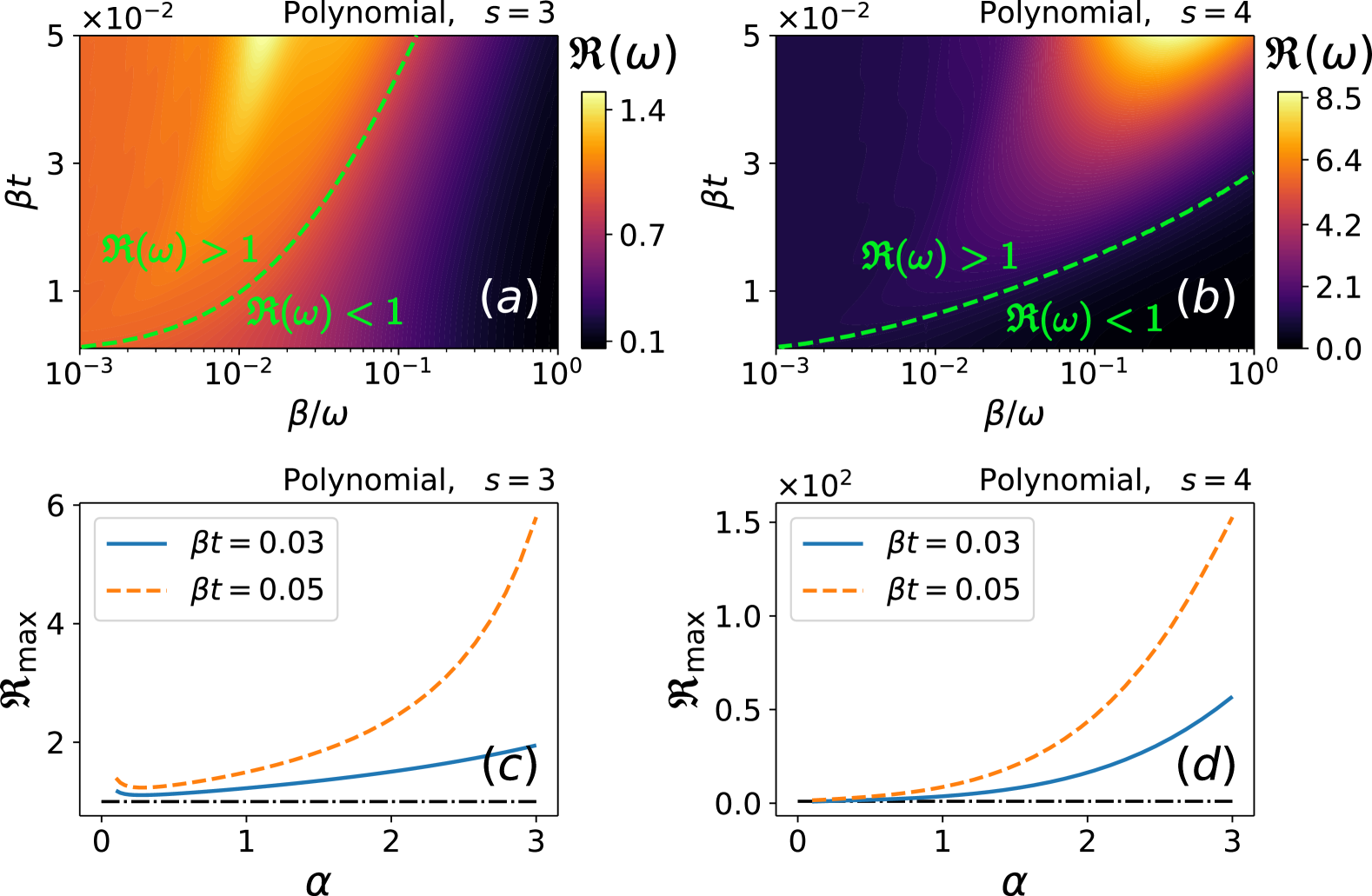
Figure 1: Polynomial case: Ratio $\mathfrak{R}(\omega)$ as functions of nonlinearity strength $\beta$ and time $t$. (a) $s{=}3$, (b) $s{=}4$. We use $\alpha{=}1$; Maximized ratio $\mathfrak{R}_{\mathrm{max}}$ as a function of $\alpha$ for different times $t$. (c) $s{=}3$, (d) $s{=}4$.

A straightforward way to increase $\mathfrak{R}(\omega)$ is by increasing the initial coherent amplitude $\alpha$. To explore how $\mathfrak{R}(\omega)$ depends on $\alpha$, we calculate:

$$\max_{0<\frac{\beta}{\omega}\leq 1}[\mathfrak{R}(\omega|\beta t)]:=\mathfrak{R}_{\mathrm{max}},$$ (6)

which maximizes the value of $\mathfrak{R}(\omega|\beta t)$ over $\beta{/}\omega$ for a given $\alpha$ and time $\beta t$. In Fig. 1(c), we plot $\mathfrak{R}_{\mathrm{max}}$ for $s{=}3$ as a function of $\alpha$ for different times $t$. Two evident conclusion can be drawn from the figure: (i) nonlinear-enhanced frequency estimation ($\mathfrak{R}_{\mathrm{max}}{>}1$) can always be achieved for any coherent input $\alpha$, with $\mathfrak{R}_{\mathrm{max}}$ increasing as both time and the coherent amplitude grow; and (ii) the growth of $\mathfrak{R}_{\mathrm{max}}$ is super-linear in $\alpha$. Note that, in Fig. 1(c), a dip in $\mathfrak{R}_{\mathrm{max}}$ is shown for $\alpha{\leq}0.5$. This can be understood as $\mathfrak{R}(\omega){\gg}1$ when $\alpha{\rightarrow}0$. Similarly, in Fig. 1(d), we plot $\mathfrak{R}_{\mathrm{max}}$ for $s{=}4$ as a function of $\alpha$ for different times $t$. As the figure shows, a significant increase in the maximized ratio $\mathfrak{R}_{\mathrm{max}}$ is achieved as time and coherent input increase.

Generalized squeezing case.— Generalized squeezing has been studied for decades in the context of quantum optics as a natural extension of standard second-order squeezing Hong and Mandel (1985); Hillery et al. (1984); D’Ariano and Rasetti (1987); Braunstein and McLachlan (1987); Banaszek and Knight (1997); Bencheikh et al. (2007), and it has been recently attained to the third order in superconducting microwave systems Chang et al. (2020). For $s{=}1$, the system reduces to the previously discussed polynomial case. For $s{=}2$, it corresponds to the well-known squeezing-driven case, where only a modest quantum enhancement in frequency estimation is observed within the parameter range considered, see SM SM for details. In Figs. 2(a)-(b), we plot $\mathfrak{R}(\omega)$ for the generalized squeezing case as functions of the nonlinearity $\beta$ and time $t$ for $s{=}3$ and $s{=}4$, respectively. As shown in Fig. 2(c), the generalized squeezing term for $s{=}3$ provides a quantum enhancement in frequency estimation comparable to the polynomial case. However, in Fig. 2(d), where $s{=}4$, significant frequency sensing enhancement is observed. To clarify this enhancement, we decompose the polynomial term in normal order as follows Louisell (1990):

$$(a^{\dagger}{+}a)^{s}{=}\sum_{k=0}^{\left[\frac{s}{2}\right]}\sum_{l=0}^{s-2k}\frac{s!}{2^{k}k!l!(s{-}2k{-}l)!}a^{\dagger s{-}2k{-}l}a^{l}.$$ (7)

In particular, for $s{=}3$ and $s{=}4$ one gets:

$$(a^{\dagger}+a)^{3} = A_{1}^{(3)}+A_{3}^{(3)},$$ (8)

$$(a^{\dagger}+a)^{4} = A_{\mathrm{ns}}^{(4)}+A_{2}^{(4)}+A_{4}^{(4)},$$ (9)

where the operators $A_{j}^{(s)}$ represents different field $j-$excitation process. We denoted with $A_{j}^{(s)}$ processes for which $A_{j}^{(s)}|n\rangle{\sim}|n{\pm}j\rangle$, and with $A_{\mathrm{ns}}^{(s)}$ processes for which $A_{\mathrm{ns}}^{(s)}|n\rangle{\sim}|n\rangle$ (where $|n\rangle$ is a Fock number state). Explicitly, for exponents $s{=}3$ one has: $A_{1}^{(3)}{=}3[a^{\dagger 2}a{+}a^{\dagger}a^{2}{+}a^{\dagger}{+}a]$ and $A_{3}^{(3)}{=}a^{\dagger 3}{+}a^{3}$; and for $s{=}4$ one has: $A_{2}^{(4)}{=}4a^{\dagger 3}a{+}4a^{\dagger}a^{3}{+}6a^{\dagger 2}{+}6a^{2}$, $A_{\mathrm{ns}}^{(4)}{=}6[(a^{\dagger}a)^{2}{+}a^{\dagger}a]$, and $A_{4}^{(4)}{=}a^{\dagger 4}{+}a^{4}$.

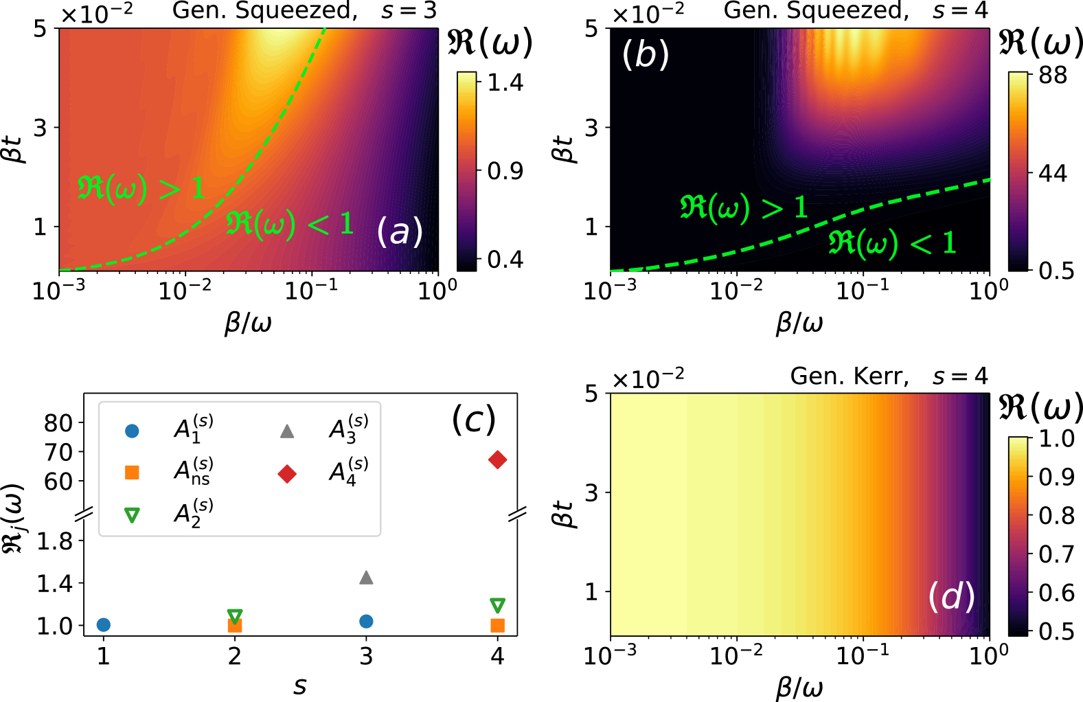
Figure 2: Generalized squeezing case: Ratio $\mathfrak{R}(\omega)$ as functions of nonlinearity strength $\beta$ and time $t$. (a) $s{=}3$, (b) $s{=}4$. (c) Ratio $\mathfrak{R}_{j}(\omega)$ as function of $s$ for several field excitation processes $A_{j}^{(s)}$. (d) Generalized Kerr case: Ratio $\mathfrak{R}(\omega)$ as functions of nonlinearity strength $\beta$ and time $t$ for $s{=}4$. We use $\alpha{=}1$.

The observed improvement in frequency estimation in the generalized squeezing scenario is likely due to the increased role of higher-order field excitation processes, as indicated by the decomposition above. To quantify this, we calculate

$$\mathfrak{R}_{j}(\omega)=\frac{\omega Q_{j}(\omega)}{4t^{2}\langle\alpha|\omega a^{\dagger}a{+}A_{j}^{(s)}|\alpha\rangle},$$ (10)

where the ratio $\mathfrak{R}_{j}(\omega)$ quantifies possible nonlinear-enhanced frequency estimation due to individual $j$-field excitation processes. Consequently, $Q_{j}(\omega)$ is the QFI computed from a initial coherent state $|\alpha\rangle$ evolved under the action of the Hamiltonian $H_{j}{=}\omega a^{\dagger}a{+}A_{j}^{(s)}$, where $j{=}\text{ns}{,}1{,}2{,}\ldots$ and $s{=}1{,}2{,}\ldots$. Recall that $A_{j}^{(s)}$ accounts for individual $j$-field excitation processes derived from the decomposition of $(a^{\dagger}{+}a)^{s}$. To ensure a fair comparison and avoid the influence of multiplicative factors in the decomposition of $A_{j}^{(s)}$, we scale all individual terms $A_{j}^{(s)}$ to have the same average energy. For simplicity, this average energy is set to $\langle A_{j}^{(s)}\rangle{=}2\alpha$ and $\beta t{=}0.05$.

In Fig. 2(c), we plot the ratio $\mathfrak{R}_{j}(\omega)$ as a function of the exponent $s$ for several field excitation processes $A_{j}^{(s)}$. The figure shows that, for a given exponent $s$, nonlinear-enhanced frequency estimation consistently occurs for higher-order field excitation processes. In addition, number state processes $A_{\mathrm{ns}}^{(s)}$ offer no sensing advantage as for $s{=}2{,}4$ the ratio $\mathfrak{R}_{j}(\omega){=}1$. This can be explained as $[a^{\dagger}a{,}A_{\mathrm{ns}}^{(s)}]{=}0$ $\forall s$, and therefore, the evolved state is $|\psi(t)\rangle{=}e^{-i\beta tA_{\mathrm{ns}}^{(s)}}|\alpha e^{-i\frac{\omega}{\beta}t}\rangle$. As the unitary operator $e^{-i\beta tA_{\mathrm{ns}}^{(s)}}$ is independent of the unknown parameter to be estimated $\omega$, the QFI cannot increase by the addition of $A_{\mathrm{ns}}^{(s)}$ in the Hamiltonian provided that $[a^{\dagger}a{,}A_{\mathrm{ns}}^{(s)}]{=}0$.

Generalized Kerr case.— The Kerr effect has also been extensively considered in quantum optics Saleh and Teich (1991) and it emerges naturally in superconducting circuits due to the nonlinear inductance of a Josephson junction Nigg et al. (2012). By using $a^{s}a^{\dagger}{=}a^{\dagger}a^{s}{+}sa^{s{-}1}$ and $aa^{\dagger s}{=}sa^{\dagger(s-1)}{+}a^{\dagger s}a$, one can straightforwardly prove that $[a^{\dagger}a{,}a^{\dagger s}a^{s}]{=}0$. Thus no sensing benefit is expected from this additional term in the Hamiltonian. To see this, in Fig. 2(d), we plot the ratio $\mathfrak{R}(\omega)$ as functions of time $t$ and nonlinearity strength $\beta$ for $s{=}4$. As the figure shows, the ratio $\mathfrak{R}(\omega){\lesssim}1$, which implies no sensing advantage under this generalized Kerr scenario. Moreover, the ratio $\mathfrak{R}(\omega)$ decreases as $\beta{/}\omega$ increases. This situation occurs because we are comparing probes that have the same average energy. Specifically, $[a^{\dagger}a{,}a^{\dagger s}a^{s}]{=}0$ ensures that the numerator in the expression for $\mathfrak{R}(\omega)$ remains unchanged, whereas the denominator in $\mathfrak{R}(\omega)$ increases as $\beta$ increases when modified to $\omega\alpha^{2}{+}\beta\alpha^{2s}$ for $\beta{\neq}0$. Thus, using a generalized Kerr term in the Hamiltonian does not provide any sensing advantage; in fact, a probe without nonlinearity is more energy-efficient.

Quantum scrambling.— Quantum scrambling has been studied across various fields, including quantum error correction Choi et al. (2020), machine learning Garcia et al. (2022); Shen et al. (2020); Wu et al. (2021); Holmes et al. (2021), chemical reactions Zhang et al. (2024), and shadow tomography Garcia et al. (2021); Hu and You (2022); McGinley et al. (2022); Hu et al. (2023); Bu et al. (2024). Several metrics for measuring quantum scrambling have been proposed, such as operator entanglement entropy Zanardi (2001); Zhou and Luitz (2017), average Pauli weight Khemani et al. (2018); Zhou and Chen (2019); Chen and Zhou (2018), and the out-of-time-ordered correlator (OTOC) Zhou and Swingle (2023); Khemani et al. (2018); Aleiner et al. (2016); Roberts and Stanford (2015); Hosur et al. (2016); Harrow et al. (2021); Nahum et al. (2018); von Keyserlingk et al. (2018). The latter, OTOC, has even been experimentally demonstrated Landsman et al. (2019); Mi et al. (2021); Li et al. (2017, 2023). Recently, a universal framework for information scrambling in open quantum systems was proposed Schuster and Yao (2023), along with its connection to quantum information thermodynamics Touil and Deffner (2020, 2024) and a resource theory that encompasses both entanglement and magic scrambling mechanisms Garcia et al. (2023).

In the field of quantum sensing, quantum information scrambling has primarily been studied using OTOCs Kobrin et al. (2024); Li et al. (2023). Here, we explore an alternative approach by focusing on the Wigner-Yanase skew information Luo (2003), which is defined as:

$$S(B,K){=}-\frac{1}{2}\mathrm{Tr}\left([\sqrt{B},K]^{2}\right),~$$ (11)

which quantifies the degree of noncommutativity between a positive operator $B$ and a fixed Hermitian operator $K$. In our context, a natural choice for these operators is $B{=}|\psi(t)\rangle\langle\psi(t)|$, representing the time-evolved state, and $K{=}a^{\dagger}a$, the number operator. The Wigner-Yanase skew information, in this case, measures the extent to which the number operator fails to commute with the evolved state. In our case, $B$ is a pure state; thus, the Wigner-Yanase skew information simplifies to:

$$S(|\psi(t)\rangle\langle\psi(t)|{,}a^{\dagger}a){=}\langle\psi(t)|(a^{\dagger}a)^{2}|\psi(t)\rangle{-}\langle\psi(t)|a^{\dagger}a|\psi(t)\rangle^{2},~$$ (12)

which is the variance of the observable $K{=}a^{\dagger}a$ in the state $|\psi(t)\rangle$. Note that, if $[H_{0}{,}H_{1}]{=}0$, then $S(|\psi(t)\rangle\langle\psi(t)|{,}a^{\dagger}a){=}|\alpha|^{2}$. In Fig. (3), we plot the skew information and the QFI as functions of the nonlinearity $\beta$ for the polynomial and generalized squeezing scenarios for $s{=}3{,}4$ at a fixed time $\beta t{=}0.05$. For clarity, the skew information is presented in arbitrary units [a. u.]. As the figure shows, the skew information fully captures the behavior of the QFI. Notably, the maximum value of the skew information (i.e., where $H_{0}$ and $H_{1}$ are maximally noncommutative) occurs near the maximum value of the QFI (i.e., where the quantum probe is most sensitive to $\omega$). A slight quantitative discrepancy arises between the two quantities. This is because Eq. (11) describes a QFI not based on SLDs; instead, it is defined as $4\mathrm{Tr}\left(\partial_{\omega}\sqrt{\rho(\omega)}\right)^{2}$ Luo (2003). Given that the skew information in Eq. (12) is computationally more tractable than the QFI, it can be used to optimize a nonlinear quantum probe with the additional Hamiltonian $H_{1}$ by decomposing it into specific transition operators $A_{j}^{(s)}$, such that (possible) time-dependent functions $f_{s}(\beta_{j}{,}t)$ can be optimized in $H{=}\omega a^{\dagger}a{+}\sum_{j}f_{s}(\beta_{j}{,}t)A_{j}^{(s)}$ for maximizing $\mathcal{R}(\omega)$. This optimization procedure makes nonlinear-enhanced frequency sensing more efficient for complex interactions where these processes dominate.

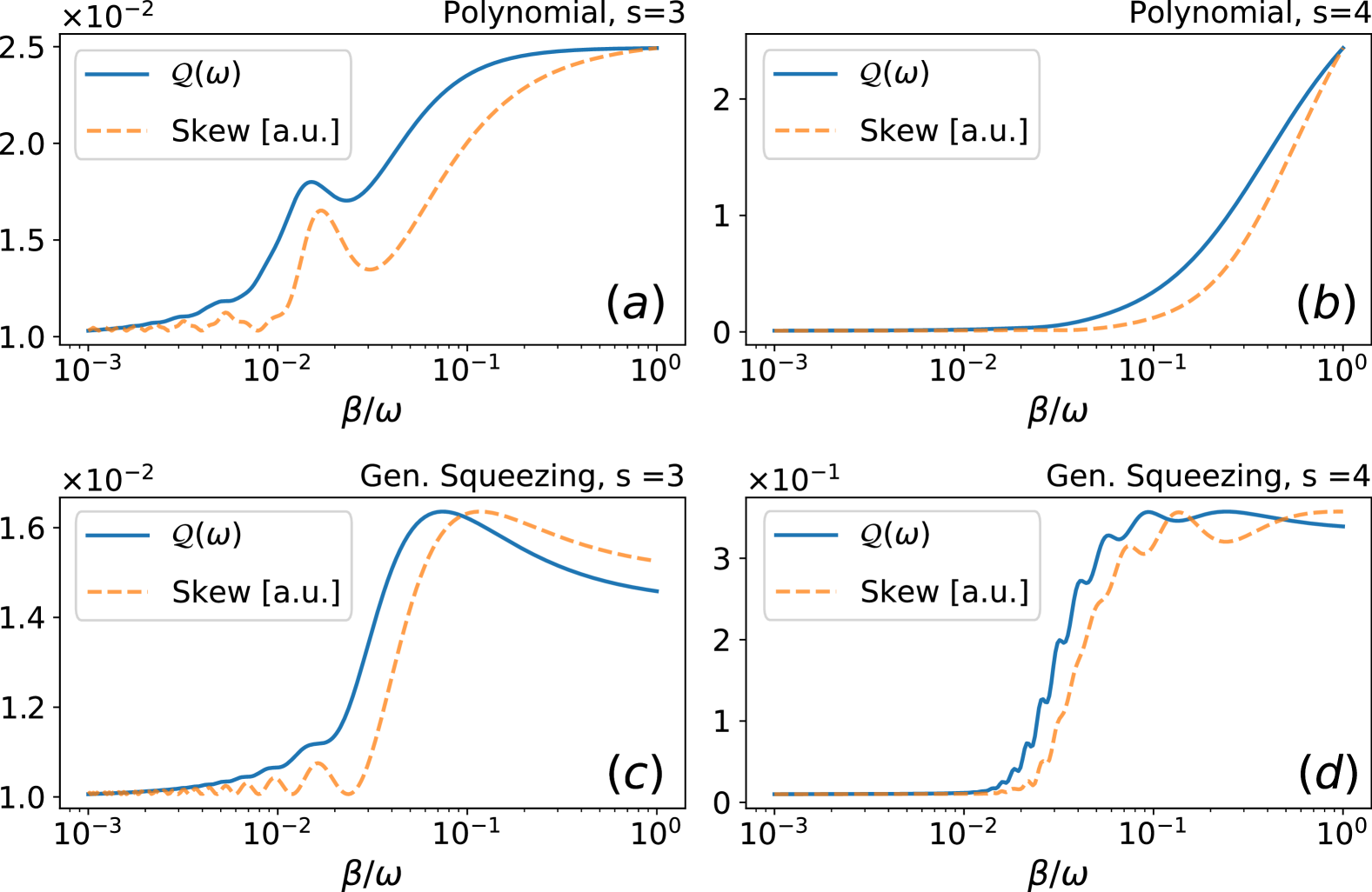
Figure 3: Skew information and the QFI as functions of the nonlinearity $\beta$ for $s{=}3{,}4$ at a fixed time $\beta t{=}0.05$. The polynomial case is shown in panels (a) and (b); The generalized squeezing case is shown in panels (c) and (d).

Conclusions.— In this Letter, we have shown that nonlinear-enhanced frequency sensing can be achieved by efficiently encoding the frequency of a quantized electromagnetic field into a nonlinear quantum probe. The introduction of nonlinearities into the quantum probe facilitates the distribution of local quantum information across a larger Hilbert space, a process referred to as quantum scrambling. To make a fair comparison between probes with and without nonlinearities, we introduced a figure of merit that ensures both probes have the same average energy. To show the generality of our findings, we examined three distinct families of nonlinear contributions. We showed that higher-order nonlinearities lead to an enhanced sensing capacity, especially in regions where the noncommutativity between the number state observable and the nonlinear contribution is maximal. As a result, we established a connection between quantum scrambling, quantified by the Wigner-Yanase skew information, and the probe’s sensitivity to slight variations in an unknown parameter, quantified by the quantum Fisher information. Our results can aid in tailoring specific nonlinear terms and can be readily generalized to other Hamiltonian parameters.

Acknowledgements.— V.M. thanks support from the National Natural Science Foundation of China Grants No. 12374482 and No. W2432005. MGAP is partially supported by EU and MIUR through the project PRIN22-2022T25TR3-RISQUE.

Supplemental Material: Enhanced quantum frequency estimation by nonlinear scrambling

Outline:

1. Frequency Estimation with a Specific Nonlinearity Contribution: Polynomial Case

2. Frequency Estimation with a General Nonlinearity Contribution: Polynomial Case for s=1,2

3. Frequency Estimation with a General Nonlinearity Contribution: Generalized Squeezing Case for s=2

4. Frequency Estimation with a General Nonlinearity Contribution: Heterodyne Sensing Performance

I I. Frequency Estimation with a Specific Nonlinearity Contribution: Polynomial Case

There is a particular situation in the polynomial case, in which the QFI can be computed analytically using coherent states. The interaction term in this case is slightly different from the one employed in the main text: assuming that the nonlinearity strength increases linearly with the frequency, the Hamiltonian takes the form:

$$H=\omega a^{\dagger}a+\omega\beta(a+a^{\dagger})^{s}\equiv\omega(a^{\dagger}a+\beta G_{s})\equiv\omega\mathcal{G}_{s}.$$ (S1)

The QFI for a coherent state that evolves according to $U(t)=e^{-iHt}$ has the simple form $Q_{s}=4t^{2}[\langle\alpha|\Delta\mathcal{G}_{s}^{2}|\alpha\rangle]$. In order to compute $Q_{s}$, the idea is to rewrite $\mathcal{G}_{s}$ and $\mathcal{G}_{s}^{2}$ in normal order, exploiting identities that can be found starting from the commutation relation $[a,a^{\dagger}]=1$, i.e.: $a^{j}a^{\dagger}=a^{\dagger}a^{j}+ja^{j-1}$, $aa^{\dagger j}=ja^{\dagger j-1}+a^{\dagger j}a$ and, in general:

$$a^{n}a^{\dagger m}=\sum_{j=0}^{\mathrm{min}[m,n]}j!\binom{n}{j}\binom{m}{j}a^{\dagger m-j}a^{n-j}.$$ (S2)

The first thing to do is to order $G_{s}$:

$$G_{s}=(a+a^{\dagger})^{s}=\sum_{k=0}^{[s/2]}\sum_{l=0}^{s-2k}\frac{s!}{2^{k}k!l!(s-2k-l)!}a^{\dagger s-2k-l}a^{l}.$$ (S3)

A complete proof of Eq. (S3) can be found in Deepak and Chatterjee (2023). Now that $\mathcal{G}_{s}$ is taken care of, it is possible to order the second term $\mathcal{G}_{s}^{2}=a^{\dagger}a+a^{\dagger 2}a^{2}+\beta a^{\dagger}aG_{s}+\beta G_{s}a^{\dagger}a+\beta^{2}G_{s}G_{s}$ using the relations above:

$$a^{\dagger}aG_{s}=\sum_{k=0}^{[s/2]}\sum_{l=0}^{s-2k}\sum_{j=0}^{\text{min}[1,s-2k-l]}j!\binom{1}{j}\binom{s-2k-l}{j}\frac{s!}{2^{k}k!l!(s-2k-l)!}a^{\dagger s-2k-l-j+1}a^{l-j+1},$$ (S4)

$$G_{s}a^{\dagger}a=\sum_{k=0}^{[s/2]}\sum_{l=0}^{s-2k}\sum_{j=0}^{\text{min}[1,l]}j!\binom{1}{j}\binom{l}{j}\frac{s!}{2^{k}k!l!(s-2k-l)!}a^{\dagger s-2k-l-j+1}a^{l-j+1},$$ (S5)

$$G_{s}G_{s}=G_{2s}=\sum_{k=0}^{s}\sum_{l=0}^{2s-2k}\frac{(2s)!}{2^{k}k!l!(2s-2k-l)!}a^{\dagger 2s-2k-l}a^{l}.$$ (S6)

In order to make clear the dependence of the QFI on the coherent state, it is useful to rewrite the complex number $\alpha$ in its exponential form $\alpha=re^{i\phi}$, where $r=|\alpha|\geq 0$ and $0\leq\phi<2\pi$.

$$Q_{1}(r,\phi,\beta) =4t^{2}[(r^{2}+2r\beta+\beta^{2})-r\beta\phi^{2}+o(\phi^{3})]$$

$$Q_{2}(r,\phi,\beta) =4t^{2}[(r^{2}+8r^{2}\beta+2\beta^{2}+16r^{2}\beta^{2})-8r^{2}\beta(1+2\beta)\phi^{2}+o(\phi^{3})]$$

$$Q_{3}(r,\phi,\beta) =4t^{2}[(r^{2}+6r\beta+24r^{3}\beta+15\beta^{2}+144r^{2}\beta^{2}+144r^{4}\beta^{2})-3r\beta(1+12r^{2}+48r\beta+96r^{3}\beta)\phi^{2}+o(\phi^{3})]$$

$$Q_{4}(r,\phi,\beta) =4t^{2}[(r^{2}+48r^{2}\beta+64r^{4}\beta+96\beta^{2}+1536r^{2}\beta^{2}+2688r^{4}\beta^{2}+1024r^{6}\beta^{2})+$$

$$-16r^{2}\beta(3+8r^{2}+96\beta+336r^{2}\beta+192r^{4}\beta)\phi^{2}+o(\phi^{3})]$$

The series expansions for $s=1,2,3,4$ show that there is a local maximum of the QFI when the phase is null. Consequently, the choice of a real $\alpha$ is not merely a simplification. From this moment on, we will always assume $\alpha$ to be real. Under this assumption, the expression for $\mathcal{G}_{s}^{2}$ can be further simplified, since the expectation values of $G_{s}a^{\dagger}a$ and $a^{\dagger}aG_{s}$ are equal. This equality follows from the fact that $(G_{s}a^{\dagger}a)^{\dagger}=a^{\dagger}aG_{s}$, which holds due to the hermiticity of $G_{s}$. Thus, the expectation value of $\mathcal{G}_{s}^{2}$ becomes:

$$\langle\alpha|\mathcal{G}_{s}^{2}|\alpha\rangle=\langle\alpha|a^{\dagger}a+a^{\dagger 2}a^{2}+2\beta a^{\dagger}aG_{s}+\beta^{2}G_{2s}|\alpha\rangle,$$ (S7)

and the final expression of the QFI is:

$$Q_{s}=4t^{2}[\alpha^{2}+2\beta\langle a^{\dagger}aG_{s}\rangle+\beta^{2}\langle G_{2s}\rangle-2\beta\alpha^{2}\langle G_{s}\rangle-\beta^{2}\langle G_{s}\rangle^{2}].$$ (S8)

As in the main text, we impose that the probes ($\beta=0$ and $\beta>0$) have the same average energy $\langle\alpha_{0}|\omega a^{\dagger}a|\alpha_{0}\rangle=\langle\alpha|\omega\mathcal{G}_{s}|\alpha\rangle$. Consequently, we obtain $\alpha_{0}=\sqrt{\alpha^{2}+\beta\langle G_{s}\rangle}$. The expansion of the ratio $\mathfrak{R}_{s}(\alpha,\beta)=\frac{Q_{s}(\alpha,\beta)}{Q_{0}(\alpha_{0})}$ for $s=1,2,3,4$ is reported below, both for small coherent amplitude $\alpha$ and small nonlinearity strength $\beta$:

The expansion with respect to small $\alpha$ in Eq. (S9a) shows that for $s=1,3$, the ratio can be made arbitrarily large with an appropriate choice of $\beta\gg\alpha$. However, this property does not hold for $s=2,4$. The expansion with respect to small $\beta$ in Eq. (S9b), shows that the ratio is equal to $1$ plus a quantity that is always positive for $s=1,3$, but can be negative for $s=2,4$. As a result, in the latter case, enhancement in frequency estimation is not universally guaranteed.

II II. Frequency Estimation with a General Nonlinearity Contribution: Polynomial case for s=1,2

Two straightforward polynomial scenarios were mentioned in the main text, namely: when the exponents are $s=1$ and $s=2$. On the one hand, for the polynomial case $s=1$, the quantum probe can be interpreted as a shift in the equilibrium position of the quantum harmonic oscillator (or as time-independent parametric external driving). Indeed, the Hamiltonian for the polynomial nonlinear case is given by $H=\omega a^{\dagger}a+\beta(a^{\dagger}+a)$, which upon switching to the position $x$ and momentum $p$ quadratures,

$$x=\sqrt{\frac{\hbar}{2\mu\omega}}(a+a^{\dagger}),\hskip 56.9055ptp=i\sqrt{\frac{\mu\hbar\omega}{2}}(a^{\dagger}-a),$$ (S10)

the Hamiltonian becomes $H\sim\frac{p^{2}}{2\mu}+\frac{\mu\omega^{2}}{2}\left(x+x_{0}\right)^{2}$, where $x_{0}=\frac{\beta}{\mu\omega^{2}}\sqrt{\frac{2\mu\omega}{\hbar}}$ is the shift of the oscillator’s equilibrium position, with $\mu$ being the effective mass of the oscillator. In this scenario, $s{=}1$, the temporal unitary operator can be found straightforwardly as Montenegro et al. (2014):

$$U(t)=D\left[\frac{\beta}{\omega}(1-e^{-i\omega t})\right]e^{-i\omega a^{\dagger}at},$$ (S11)

where $D[z]=\exp(za^{\dagger}-z^{*}a)$ is the displacement operator. Therefore, an initial coherent state $|\alpha\rangle$ evolves as:

$$|\psi(t)\rangle_{s=1}=\left|\alpha e^{-i\omega t}+\frac{\beta}{\omega}\left(1-e^{-i\omega t}\right)\right\rangle,$$ (S12)

which is the expression shown in the main text. Using Eq. (S12), the quantum Fisher information (QFI) $Q(\omega)$ with respect to $\omega$ can be directly evaluated. Consequently, the QFI ratio $\mathfrak{R}(\omega)$ is:

$$\mathfrak{R}(\omega)=\frac{\omega Q(\omega)}{4t^{2}\langle\alpha{|}H{|}\alpha\rangle}=\frac{2\alpha\beta t^{2}\omega^{3}+\alpha^{2}t^{2}\omega^{4}+\beta^{2}(2+t^{2}\omega^{2})-2\beta^{2}\cos(t\omega)-2\beta t\omega(\beta+\alpha\omega)\sin(t\omega)}{t^{2}\omega^{3}(2\alpha\beta+\alpha^{2}\omega)}.$$ (S13)

In Fig. S1(a), we plot the QFI ratio $\mathfrak{R}(\omega)$ for the polynomial case $s{=}1$ as functions of time $\beta t$ and the nonlinearity strength $\beta/\omega$. As the figure shows, within the range of parameters considered in this work, the QFI ratio indicates no enhancements in frequency estimation, namely: $\mathfrak{R}(\omega)\leq 1$. The latter corresponds to the claim presented in the main text.

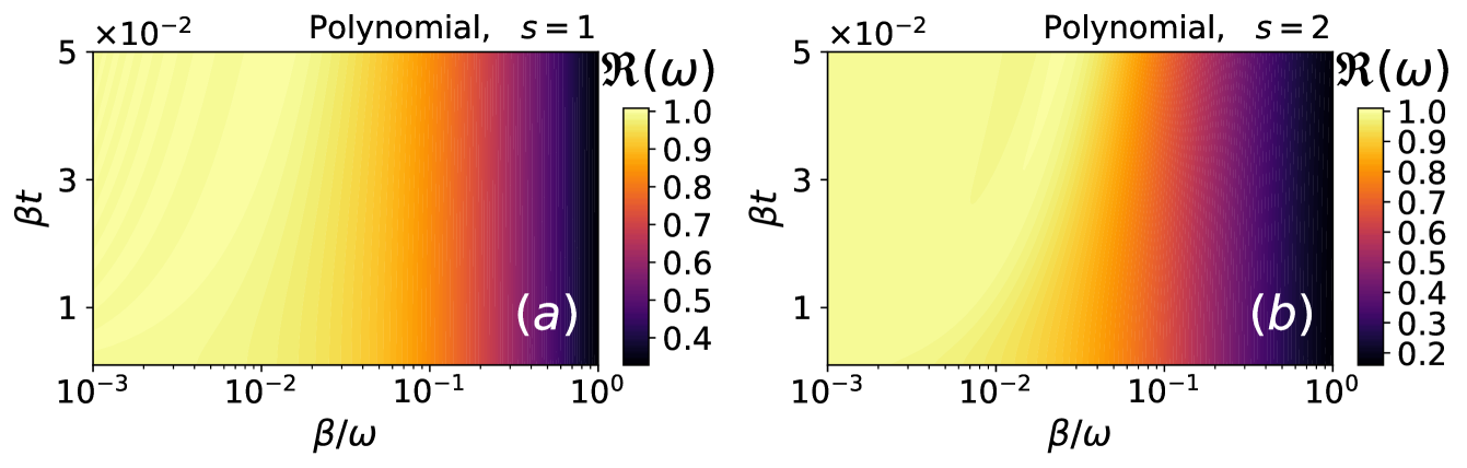
Figure S1: QFI ratio $\mathfrak{R}(\omega)$ for the polynomial case as functions of time $\beta t$ and the nonlinearity strength $\beta/\omega$. No enhancements in frequency estimation is reported, namely: $\mathfrak{R}(\omega)\leq 1$. (a) $s{=}1$, (b) $s{=}2$.

On the other hand, for the polynomial case $s=2$, the quantum probe can be interpreted as squeezing induced by modulation of the oscillator’s frequency. Here, the Hamiltonian is $H=\omega a^{\dagger}a+\beta(a^{\dagger}+a)^{2}\sim(\omega+2\beta)a^{\dagger}a+\beta a^{\dagger 2}+\beta a^{2}$. The above Hamiltonian can be readily diagonalized using a Bogoliubov transformation or by rewriting the Hamiltonian in terms of the position $x$ and momentum $p$ [see Eqs. (S10)]. Hence:

$$H=\frac{p^{2}}{2\mu}+\frac{1}{2}\mu\omega^{2}x^{2}+\frac{1}{2}\mu\omega^{\prime 2}x^{2}.$$ (S14)

In this formulation, the polynomial nonlinear term $\beta(a^{\dagger}+a)^{2}=\frac{\hbar w^{\prime 2}}{4\omega}(a^{\dagger}+a)^{2}$ translates directly into an additional quadratic potential proportional to $x^{2}$. By combining the coefficients of $x^{2}$, the effective frequency of the oscillator is modified. The resulting diagonalized Hamiltonian becomes:

$$H\sim\frac{p^{2}}{2\mu}+\frac{1}{2}\mu\omega_{\text{eff}}^{2}x^{2}=\hbar\omega_{\text{eff}}b^{\dagger}b=\hbar\sqrt{\omega^{2}+4\omega\beta}b^{\dagger}b,$$ (S15)

where $x=\sqrt{\frac{\hbar}{2\mu\omega_{\text{eff}}}}(b+b^{\dagger}),p=i\sqrt{\frac{\mu\hbar\omega_{\text{eff}}}{2}}(b^{\dagger}-b)$. Eq. (S15) coincides with the one presented in the main text.

Solutions for the temporal unitary operator can be obtained using a Lie algebraic approach Qvarfort and Pikovski (2022). However, a closed analytical form for the evolution of an initial coherent state under $H=\omega a^{\dagger}a+\beta(a^{\dagger}+a)^{2}$ is not attainable. In Fig. S1(b), we numerically evaluate the QFI ratio $\mathfrak{R}(\omega)$ for the polynomial case $s{=}2$ as functions of time $\beta t$ and the nonlinearity strength $\beta/\omega$. As seen in the figure, within the range of parameters considered in this work, the QFI ratio indicates no enhancements in frequency estimation, namely $\mathfrak{R}(\omega)\leq 1$. This supports our claim in the main text for this specific case.

III III. Frequency Estimation with a General Nonlinearity Contribution: Generalized squeezing case for s=2

In contrast to the previous polynomial scenario, for the generalized squeezing case $H=\omega a^{\dagger}a+\beta a^{\dagger 2}+\beta a^{2}$, the number state contribution depends only on the frequency we aim to estimate and is not affected by additional nonlinearities $\beta$. This implies that: (i) the Hamiltonian for the generalized squeezing case $s=2$ cannot be rewritten as being proportional to $\sim b^{\dagger}b$; and (ii) increasing the nonlinearity only enhances the two-field excitation process. In contrast, for the polynomial case, both the number state subspace and the two-field excitation process are modified as the nonlinearity increases. In Fig. S2(a), we numerically compute the QFI ratio $\mathfrak{R}(\omega)$ for the generalized squeezing case $s{=}2$ as functions of time $\beta t$ and the nonlinearity strength $\beta/\omega$. As shown in the figure, within the range of parameters considered in this work, the QFI ratio shows negligible nonlinear-enhanced frequency estimation $\mathfrak{R}(\omega)\sim 1$. Note that, for the case $s=2$, by increasing the time $\beta t$, one can achieve higher values of $\mathfrak{R}(\omega)$ (not shown in the figure). Nonetheless, these values would fall outside current experimental capabilities. Therefore, we restrict ourselves to exploring the set of parameters within experimental reach, namely $\beta t\leq 0.05$ and $\beta\leq\omega$. Further studies involving longer times and stronger nonlinearities could be explored in future work.

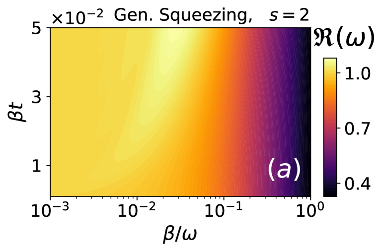
Figure S2: QFI ratio $\mathfrak{R}(\omega)$ for the generalized squeezing case $s{=}2$ as functions of time $\beta t$ and the nonlinearity strength $\beta/\omega$.

IV IV. Frequency Estimation with a General Nonlinearity Contribution: Heterodyne sensing performance

Any sensing protocol relies on performing measurements on the probe to extract information about the parameters of interest. The outcomes of these measurements are used to construct probability distributions, which are then used to build the classical Fisher information (CFI). As discussed in the “Quantum Metrological Tools” section, the symmetric logarithmic derivatives (SLDs) $L(\omega)$ define the optimal measurement basis required to achieve the ultimate sensing precision, quantified by the quantum Fisher information (QFI) $Q(\omega):=\mathrm{Tr}[\partial_{\omega}\rho(\omega)L(\omega)]$. However, while the optimal measurement (based on the eigenstates of the SLDs) is theoretically well-defined Paris (2009), in practice, such measurements are often highly correlated and challenging to implement. Therefore, it is far more informative to establish the sensing precision for a given feasible measurement basis, which in the case of the electromagnetic field is typically limited to photocounting, homodyne detection, and heterodyne detection. Given the large Hilbert space due to the presence of $H_{1}$, heterodyne detection can be efficiently simulated using probability distributions

$$p(\Upsilon{|}\omega){=}\frac{1}{\pi}\text{Tr}[|\Upsilon\rangle\langle\Upsilon|\psi(t)\rangle\langle\psi(t)|],$$ (S16)

where $|\Upsilon\rangle$ a coherent state with complex amplitude. Hence, the CFI, see “Quantum Metrological Tools” section, is:

$$\mathcal{F}(\omega)^{\mathrm{Heterodyne}}=\int d^{2}\Upsilon p(\Upsilon|\omega)\left[\partial_{\omega}\ln p(\Upsilon|\omega)\right]^{2}.$$ (S17)

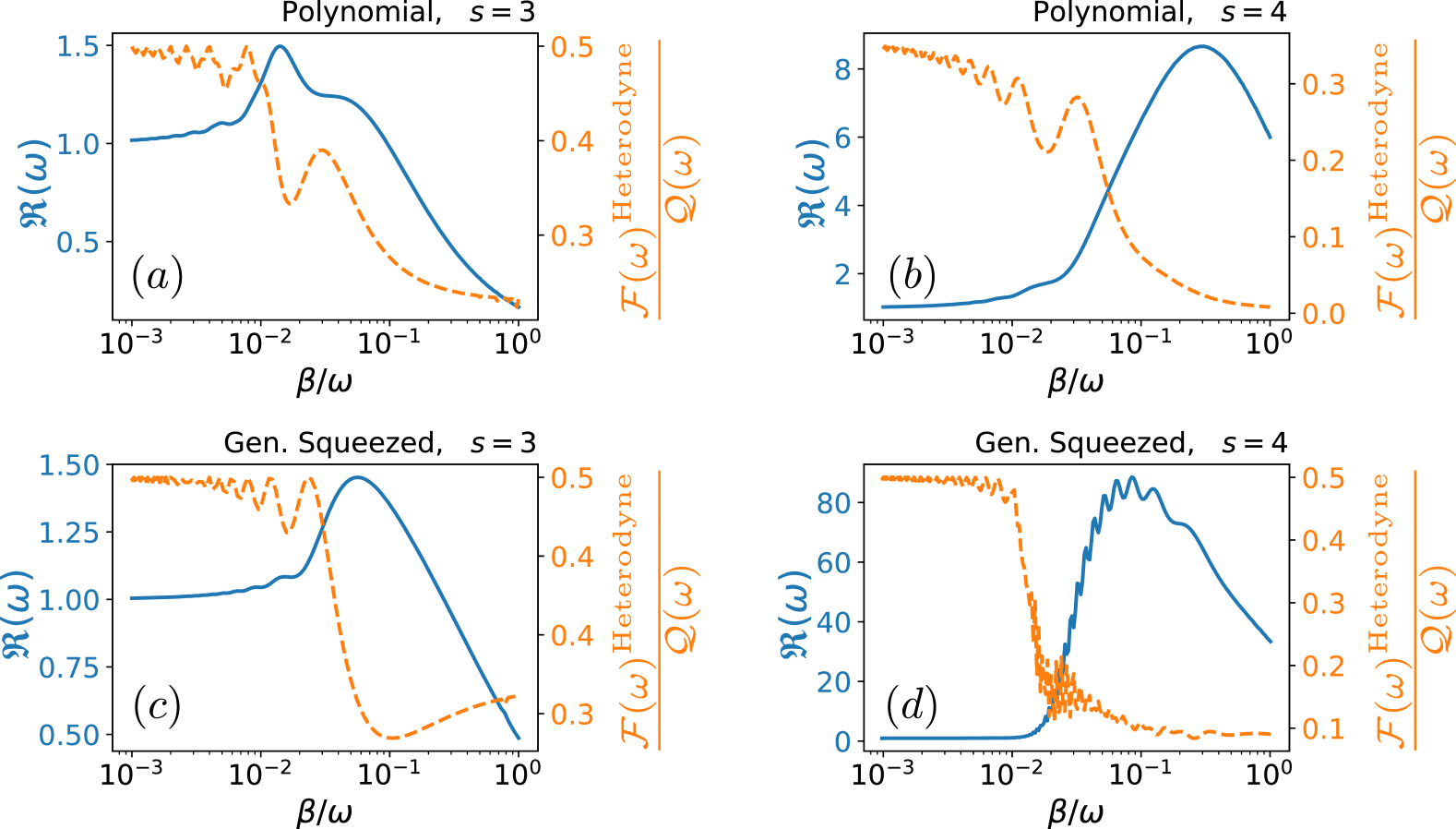
Figure S3: Heterodyne performance ratio $\mathcal{F}(\omega)^{\mathrm{Heterodyne}}/Q(\omega)$ as a function of the nonlinearity strength $\beta$. Panels (a) and (b), polynomial case for $s=3$ and $s=4$. Panels (c) and (d), generalized squeezing case for $s=3$ and $s=4$. For reference, we show the QFI ratio $\mathcal{R}(\omega)$. We set $\beta t=0.05$ and the initial coherent amplitude $\alpha=1$.

To assess the sensing performance of heterodyne detection, we calculate the ratio between the CFI obtained from heterodyne detection and the QFI: $\mathcal{F}(\omega)^{\mathrm{Heterodyne}}/Q(\omega)$. In Fig. S3, we plot $\mathcal{F}(\omega)^{\mathrm{Heterodyne}}/Q(\omega)$ as a function of the nonlinearity strength $\beta$ for both the polynomial and generalized squeezing scenarios. For reference, we also include the QFI ratio $\mathcal{R}(\omega)$. Panels (a) and (b) show $\mathcal{F}(\omega)^{\mathrm{Heterodyne}}/Q(\omega)$ for the polynomial case with $s{=}3$ and $s{=}4$, respectively. As shown in the figure, the performance of heterodyne detection decreases as the nonlinearity $\beta$ increases. Specifically, at the point where the QFI ratio $\mathcal{R}(\omega)$ reaches its maximum—corresponding to the highest degree of nonlinear-enhanced frequency estimation attainable for the given probe with a specific $s$ and time $\beta t$—heterodyne detection captures only a fraction of the available information. For $s=3$, this fraction is approximately $0.3$, while for $s=4$, it drops significantly to about $0.02$. Panels (c) and (d) show the fraction $\mathcal{F}(\omega)^{\mathrm{Heterodyne}}/Q(\omega)$ for the generalized squeezing case with $s{=}3$ and $s{=}4$, respectively. As seen from the figure, for $s=3$, this fraction is approximately $0.3$ (comparable to the polynomial case), while for $s=4$, it drops to about $0.1$. Note that for the generalized squeezing case, the QFI ratio is significantly larger than that of the polynomial case. Nonetheless, as evidenced by the heterodyne performance, it is possible to achieve improved sensing capabilities for the generalized squeezing case using a feasible heterodyne detection scheme.

References

- Gisin and Thew (2007) Nicolas Gisin and Rob Thew, “Quantum communication,” Nature Photonics 1, 165–171 (2007).
- Chen (2021) Jiajun Chen, “Review on quantum communication and quantum computation,” Journal of Physics: Conference Series 1865, 022008 (2021).
- Degen et al. (2017) C. L. Degen, F. Reinhard, and P. Cappellaro, “Quantum sensing,” Rev. Mod. Phys. 89, 035002 (2017).
- Pirandola et al. (2018) S. Pirandola, B. R. Bardhan, T. Gehring, C. Weedbrook, and S. Lloyd, “Advances in photonic quantum sensing,” Nature Photonics 12, 724–733 (2018).
- Montenegro et al. (2024) Victor Montenegro, Chiranjib Mukhopadhyay, Rozhin Yousefjani, Saubhik Sarkar, Utkarsh Mishra, Matteo G. A. Paris, and Abolfazl Bayat, “Review: Quantum metrology and sensing with many-body systems,” (2024), arXiv:2408.15323 [quant-ph] .
- Aharonov (1999) D. Aharonov, “Quantum computation,” in Annual Reviews of Computational Physics VI (World Scientific, 1999) p. 259–346.
- Giovannetti et al. (2004) Vittorio Giovannetti, Seth Lloyd, and Lorenzo Maccone, “Quantum-enhanced measurements: beating the standard quantum limit,” Science 306, 1330–1336 (2004).
- Giovannetti et al. (2006) Vittorio Giovannetti, Seth Lloyd, and Lorenzo Maccone, “Quantum metrology,” Phys. Rev. Lett. 96, 010401 (2006).
- Giovannetti et al. (2011) Vittorio Giovannetti, Seth Lloyd, and Lorenzo Maccone, “Advances in quantum metrology,” Nature photonics 5, 222–229 (2011).
- Udem et al. (2002) Th. Udem, R. Holzwarth, and T. W. Hänsch, “Optical frequency metrology,” Nature 416, 233–237 (2002).
- Descamps et al. (2023) Eloi Descamps, Nicolas Fabre, Arne Keller, and Pérola Milman, “Quantum metrology using time-frequency as quantum continuous variables: Resources, sub-shot-noise precision and phase space representation,” Phys. Rev. Lett. 131, 030801 (2023).
- Kuenstner et al. (2024) Stephen E. Kuenstner, Elizabeth C. van Assendelft, Saptarshi Chaudhuri, Hsiao-Mei Cho, Jason Corbin, Shawn W. Henderson, Fedja Kadribasic, Dale Li, Arran Phipps, Nicholas M. Rapidis, Maria Simanovskaia, Jyotirmai Singh, Cyndia Yu, and Kent D. Irwin, “Quantum metrology of low frequency electromagnetic modes with frequency upconverters,” (2024), arXiv:2210.05576 [quant-ph] .
- Boss et al. (2017) J. M. Boss, K. S. Cujia, J. Zopes, and C. L. Degen, “Quantum sensing with arbitrary frequency resolution,” Science 356, 837–840 (2017).
- Cai et al. (2021) Y. Cai, J. Roslund, V. Thiel, C. Fabre, and N. Treps, “Quantum enhanced measurement of an optical frequency comb,” npj Quantum Information 7, 82 (2021).
- Roos et al. (2006) C. F. Roos, M. Chwalla, K. Kim, M. Riebe, and R. Blatt, “‘designer atoms’ for quantum metrology,” Nature 443, 316–319 (2006).
- Schmitt et al. (2021) Simon Schmitt, Tuvia Gefen, Daniel Louzon, Christian Osterkamp, Nicolas Staudenmaier, Johannes Lang, Matthew Markham, Alex Retzker, Liam P. McGuinness, and Fedor Jelezko, “Optimal frequency measurements with quantum probes,” npj Quantum Information 7, 55 (2021).
- Lamperti et al. (2020) M. Lamperti, R. Gotti, D. Gatti, M. K. Shakfa, E. Cané, F. Tamassia, P. Schunemann, P. Laporta, A. Farooq, and M. Marangoni, “Optical frequency metrology in the bending modes region,” Communications Physics 3, 175 (2020).
- Ludlow et al. (2015) Andrew D. Ludlow, Martin M. Boyd, Jun Ye, E. Peik, and P. O. Schmidt, “Optical atomic clocks,” Rev. Mod. Phys. 87, 637–701 (2015).
- Haase et al. (2018) J F Haase, A Smirne, J Kołodyński, R Demkowicz-Dobrzański, and S F Huelga, “Fundamental limits to frequency estimation: a comprehensive microscopic perspective,” New Journal of Physics 20, 053009 (2018).
- Bollinger et al. (1996) J. J . Bollinger, Wayne M. Itano, D. J. Wineland, and D. J. Heinzen, “Optimal frequency measurements with maximally correlated states,” Phys. Rev. A 54, R4649–R4652 (1996).
- Dorner (2012) U Dorner, “Quantum frequency estimation with trapped ions and atoms,” New Journal of Physics 14, 043011 (2012).
- Albarelli et al. (2018) Francesco Albarelli, Matteo A. C. Rossi, Dario Tamascelli, and Marco G. Genoni, “Restoring Heisenberg scaling in noisy quantum metrology by monitoring the environment,” Quantum 2, 110 (2018).
- Albarelli et al. (2020) Francesco Albarelli, Matteo A. C. Rossi, and Marco G. Genoni, “Quantum frequency estimation with conditional states of continuously monitored independent dephasing channels,” International Journal of Quantum Information 18, 1941013 (2020).
- Naghiloo et al. (2017) M. Naghiloo, A. N. Jordan, and K. W. Murch, “Achieving optimal quantum acceleration of frequency estimation using adaptive coherent control,” Phys. Rev. Lett. 119, 180801 (2017).
- Rodríguez-García et al. (2024) Marco A. Rodríguez-García, Ruynet L. de Matos Filho, and Pablo Barberis-Blostein, “Usefulness of quantum entanglement for enhancing precision in frequency estimation,” Phys. Rev. Res. 6, 043230 (2024).
- Huelga et al. (1997) S. F. Huelga, C. Macchiavello, T. Pellizzari, A. K. Ekert, M. B. Plenio, and J. I. Cirac, “Improvement of frequency standards with quantum entanglement,” Phys. Rev. Lett. 79, 3865–3868 (1997).
- Smirne et al. (2016) Andrea Smirne, Jan Kołodyński, Susana F. Huelga, and Rafał Demkowicz-Dobrzański, “Ultimate precision limits for noisy frequency estimation,” Phys. Rev. Lett. 116, 120801 (2016).
- Haase et al. (2016) J. F. Haase, A. Smirne, S. F. Huelga, J. Kołodynski, and R. Demkowicz-Dobrzanski, “Precision limits in quantum metrology with open quantum systems,” Quantum Measurements and Quantum Metrology 5, 13–39 (2016).
- Macieszczak et al. (2014) Katarzyna Macieszczak, Martin Fraas, and Rafał Demkowicz-Dobrzański, “Bayesian quantum frequency estimation in presence of collective dephasing,” New Journal of Physics 16, 113002 (2014).
- Macieszczak (2015) Katarzyna Macieszczak, “Zeno limit in frequency estimation with non-markovian environments,” Phys. Rev. A 92, 010102 (2015).
- Donohue et al. (2018) J. M. Donohue, V. Ansari, J. Řeháček, Z. Hradil, B. Stoklasa, M. Paúr, L. L. Sánchez-Soto, and C. Silberhorn, “Quantum-limited time-frequency estimation through mode-selective photon measurement,” Phys. Rev. Lett. 121, 090501 (2018).
- Fröwis et al. (2014) F Fröwis, M Skotiniotis, B Kraus, and W Dür, “Optimal quantum states for frequency estimation,” New Journal of Physics 16, 083010 (2014).
- Helstrom (1969) Carl W Helstrom, “Quantum detection and estimation theory,” J. Stat. Phys. 1, 231–252 (1969).
- Paris (2009) Matteo G. A. Paris, “Quantum estimation for quantum technology,” International Journal of Quantum Information 07, 125–137 (2009).
- Liuzzo-Scorpo et al. (2018) Pietro Liuzzo-Scorpo, Luis A Correa, Felix A Pollock, Agnieszka Górecka, Kavan Modi, and Gerardo Adesso, “Energy-efficient quantum frequency estimation,” New Journal of Physics 20, 063009 (2018).
- Garcia et al. (2023) Roy J. Garcia, Kaifeng Bu, and Arthur Jaffe, “Resource theory of quantum scrambling,” Proceedings of the National Academy of Sciences 120, e2217031120 (2023).
- Zanardi (2001) Paolo Zanardi, “Entanglement of quantum evolutions,” Phys. Rev. A 63, 040304 (2001).
- Zhou and Luitz (2017) Tianci Zhou and David J. Luitz, “Operator entanglement entropy of the time evolution operator in chaotic systems,” Phys. Rev. B 95, 094206 (2017).
- Khemani et al. (2018) Vedika Khemani, Ashvin Vishwanath, and David A. Huse, “Operator spreading and the emergence of dissipative hydrodynamics under unitary evolution with conservation laws,” Phys. Rev. X 8, 031057 (2018).
- Chen and Zhou (2018) Xiao Chen and Tianci Zhou, “Operator scrambling and quantum chaos,” (2018), arXiv:1804.08655 [cond-mat.str-el] .
- Zhou and Swingle (2023) Tianci Zhou and Brian Swingle, “Operator growth from global out-of-time-order correlators,” Nature Communications 14, 3411 (2023).
- Aleiner et al. (2016) Igor L. Aleiner, Lara Faoro, and Lev B. Ioffe, “Microscopic model of quantum butterfly effect: Out-of-time-order correlators and traveling combustion waves,” Annals of Physics 375, 378–406 (2016).
- Harrow et al. (2021) Aram W. Harrow, Linghang Kong, Zi-Wen Liu, Saeed Mehraban, and Peter W. Shor, “Separation of out-of-time-ordered correlation and entanglement,” PRX Quantum 2, 020339 (2021).
- Nahum et al. (2018) Adam Nahum, Sagar Vijay, and Jeongwan Haah, “Operator spreading in random unitary circuits,” Phys. Rev. X 8, 021014 (2018).
- von Keyserlingk et al. (2018) C. W. von Keyserlingk, Tibor Rakovszky, Frank Pollmann, and S. L. Sondhi, “Operator hydrodynamics, otocs, and entanglement growth in systems without conservation laws,” Phys. Rev. X 8, 021013 (2018).
- Touil and Deffner (2024) Akram Touil and Sebastian Deffner, “Information scrambling —a quantum thermodynamic perspective,” Europhysics Letters 146, 48001 (2024).
- Touil and Deffner (2020) Akram Touil and Sebastian Deffner, “Quantum scrambling and the growth of mutual information,” Quantum Science and Technology 5, 035005 (2020).
- Kobrin et al. (2024) Bryce Kobrin, Thomas Schuster, Maxwell Block, Weijie Wu, Bradley Mitchell, Emily Davis, and Norman Y. Yao, “A universal protocol for quantum-enhanced sensing via information scrambling,” (2024), arXiv:2411.12794 [quant-ph] .
- Li et al. (2023) Zeyang Li, Simone Colombo, Chi Shu, Gustavo Velez, Saúl Pilatowsky-Cameo, Roman Schmied, Soonwon Choi, Mikhail Lukin, Edwin Pedrozo-Peñafiel, and Vladan Vuletić, “Improving metrology with quantum scrambling,” Science 380, 1381–1384 (2023).
- Wigner and Yanase (1963) E. P. Wigner and Mutsuo M. Yanase, “Information contents of distributions,” Proceedings of the National Academy of Sciences 49, 910–918 (1963).
- Luo (2003) Shunlong Luo, “Wigner-yanase skew information and uncertainty relations,” Phys. Rev. Lett. 91, 180403 (2003).
- Chen (2005) Zeqian Chen, “Wigner-yanase skew information as tests for quantum entanglement,” Phys. Rev. A 71, 052302 (2005).
- Chen and Lian (2023) Bin Chen and Pan Lian, “Geometric uncertainty relations on wigner–yanase skew information,” Journal of Physics A: Mathematical and Theoretical 56, 275301 (2023).
- Luo and Zhang (2019) Shunlong Luo and Yue Zhang, “Quantifying nonclassicality via wigner-yanase skew information,” Phys. Rev. A 100, 032116 (2019).
- Takagi (2019) Ryuji Takagi, “Skew informations from an operational view via resource theory of asymmetry,” Scientific Reports 9, 14562 (2019).
- Luo et al. (2012) Shunlong Luo, Shuangshuang Fu, and Choo Hiap Oh, “Quantifying correlations via the wigner-yanase skew information,” Phys. Rev. A 85, 032117 (2012).
- Cramér (1999) Harald Cramér, Mathematical methods of statistics, Vol. 26 (Princeton university press, 1999).
- Rao (1992) C. Radhakrishna Rao, “Information and the accuracy attainable in the estimation of statistical parameters,” in Breakthroughs in Statistics: Foundations and Basic Theory, edited by Samuel Kotz and Norman L. Johnson (Springer New York, New York, NY, 1992) pp. 235–247.
- Helstrom (1967) Carl W Helstrom, “Minimum mean-squared error of estimates in quantum statistics,” Physics letters A 25, 101–102 (1967).
- Liu et al. (2016) Jing Liu, Jie Chen, Xiao-Xing Jing, and Xiaoguang Wang, “Quantum fisher information and symmetric logarithmic derivative via anti-commutators,” Journal of Physics A: Mathematical and Theoretical 49, 275302 (2016).
- Braunstein and Caves (1994) Samuel L. Braunstein and Carlton M. Caves, “Statistical distance and the geometry of quantum states,” Physical Review Letters 72, 3439–3443 (1994).
- Sidhu and Kok (2020) Jasminder S Sidhu and Pieter Kok, “Geometric perspective on quantum parameter estimation,” AVS Quantum Science 2, 014701 (2020).
- (63) Supplemental Material.
- Hillmann et al. (2020) Timo Hillmann, Fernando Quijandría, Göran Johansson, Alessandro Ferraro, Simone Gasparinetti, and Giulia Ferrini, “Universal gate set for continuous-variable quantum computation with microwave circuits,” Physical review letters 125, 160501 (2020).
- Eriksson et al. (2024) Axel M Eriksson, Théo Sépulcre, Mikael Kervinen, Timo Hillmann, Marina Kudra, Simon Dupouy, Yong Lu, Maryam Khanahmadi, Jiaying Yang, Claudia Castillo-Moreno, et al., “Universal control of a bosonic mode via drive-activated native cubic interactions,” Nature Communications 15, 2512 (2024).
- Hong and Mandel (1985) CK Hong and L Mandel, “Higher-order squeezing of a quantum field,” Physical review letters 54, 323 (1985).
- Hillery et al. (1984) Mark Hillery, MS Zubairy, and K Wodkiewicz, “Squeezing in higher order nonlinear optical processes,” Physics Letters A 103, 259–261 (1984).
- D’Ariano and Rasetti (1987) G D’Ariano and Mario Rasetti, “Non-gaussian multiphoton squeezed states,” Physical Review D 35, 1239 (1987).
- Braunstein and McLachlan (1987) Samuel L Braunstein and Robert I McLachlan, “Generalized squeezing,” Physical Review A 35, 1659 (1987).
- Banaszek and Knight (1997) Konrad Banaszek and Peter L Knight, “Quantum interference in three-photon down-conversion,” Physical Review A 55, 2368 (1997).
- Bencheikh et al. (2007) Kamel Bencheikh, Fabien Gravier, Julien Douady, Ariel Levenson, and Benoît Boulanger, “Triple photons: a challenge in nonlinear and quantum optics,” Comptes Rendus. Physique 8, 206–220 (2007).
- Chang et al. (2020) CW Sandbo Chang, Carlos Sabín, P Forn-Díaz, Fernando Quijandría, AM Vadiraj, I Nsanzineza, Göran Johansson, and CM Wilson, “Observation of three-photon spontaneous parametric down-conversion in a superconducting parametric cavity,” Physical Review X 10, 011011 (2020).
- Louisell (1990) William H. Louisell, Quantum statistical properties of radiation, Wiley Classics Library (Wiley-Interscience, 1990).
- Saleh and Teich (1991) Bahaa EA Saleh and Malvin Carl Teich, Fundamentals of photonics (John Wiley & Sons, 1991).
- Nigg et al. (2012) Simon E Nigg, Hanhee Paik, Brian Vlastakis, Gerhard Kirchmair, Shyam Shankar, Luigi Frunzio, MH Devoret, RJ Schoelkopf, and SM Girvin, “Black-box superconducting circuit quantization,” Physical Review Letters 108, 240502 (2012).
- Choi et al. (2020) Soonwon Choi, Yimu Bao, Xiao-Liang Qi, and Ehud Altman, “Quantum error correction in scrambling dynamics and measurement-induced phase transition,” Phys. Rev. Lett. 125, 030505 (2020).
- Garcia et al. (2022) Roy J. Garcia, Kaifeng Bu, and Arthur Jaffe, “Quantifying scrambling in quantum neural networks,” Journal of High Energy Physics 2022, 27 (2022).
- Shen et al. (2020) Huitao Shen, Pengfei Zhang, Yi-Zhuang You, and Hui Zhai, “Information scrambling in quantum neural networks,” Phys. Rev. Lett. 124, 200504 (2020).
- Wu et al. (2021) Yadong Wu, Pengfei Zhang, and Hui Zhai, “Scrambling ability of quantum neural network architectures,” Phys. Rev. Res. 3, L032057 (2021).
- Holmes et al. (2021) Zoë Holmes, Andrew Arrasmith, Bin Yan, Patrick J. Coles, Andreas Albrecht, and Andrew T. Sornborger, “Barren plateaus preclude learning scramblers,” Phys. Rev. Lett. 126, 190501 (2021).
- Zhang et al. (2024) Chenghao Zhang, Sohang Kundu, Nancy Makri, Martin Gruebele, and Peter G. Wolynes, “Quantum information scrambling and chemical reactions,” Proceedings of the National Academy of Sciences 121, e2321668121 (2024).
- Garcia et al. (2021) Roy J. Garcia, You Zhou, and Arthur Jaffe, “Quantum scrambling with classical shadows,” Phys. Rev. Res. 3, 033155 (2021).
- Hu and You (2022) Hong-Ye Hu and Yi-Zhuang You, “Hamiltonian-driven shadow tomography of quantum states,” Phys. Rev. Res. 4, 013054 (2022).
- McGinley et al. (2022) Max McGinley, Sebastian Leontica, Samuel J. Garratt, Jovan Jovanovic, and Steven H. Simon, “Quantifying information scrambling via classical shadow tomography on programmable quantum simulators,” Phys. Rev. A 106, 012441 (2022).
- Hu et al. (2023) Hong-Ye Hu, Soonwon Choi, and Yi-Zhuang You, “Classical shadow tomography with locally scrambled quantum dynamics,” Phys. Rev. Res. 5, 023027 (2023).
- Bu et al. (2024) Kaifeng Bu, Dax Enshan Koh, Roy J. Garcia, and Arthur Jaffe, “Classical shadows with pauli-invariant unitary ensembles,” npj Quantum Information 10, 6 (2024).
- Zhou and Chen (2019) Tianci Zhou and Xiao Chen, “Operator dynamics in a brownian quantum circuit,” Phys. Rev. E 99, 052212 (2019).
- Roberts and Stanford (2015) Daniel A. Roberts and Douglas Stanford, “Diagnosing chaos using four-point functions in two-dimensional conformal field theory,” Phys. Rev. Lett. 115, 131603 (2015).
- Hosur et al. (2016) Pavan Hosur, Xiao-Liang Qi, Daniel A. Roberts, and Beni Yoshida, “Chaos in quantum channels,” Journal of High Energy Physics 2016, 4 (2016).
- Landsman et al. (2019) K. A. Landsman, C. Figgatt, T. Schuster, N. M. Linke, B. Yoshida, N. Y. Yao, and C. Monroe, “Verified quantum information scrambling,” Nature 567, 61–65 (2019).
- Mi et al. (2021) Xiao Mi, Pedram Roushan, Chris Quintana, Salvatore Mandrà, Jeffrey Marshall, Charles Neill, Frank Arute, Kunal Arya, Juan Atalaya, Ryan Babbush, Joseph C. Bardin, Rami Barends, Joao Basso, Andreas Bengtsson, Sergio Boixo, Alexandre Bourassa, Michael Broughton, Bob B. Buckley, David A. Buell, Brian Burkett, Nicholas Bushnell, Zijun Chen, Benjamin Chiaro, Roberto Collins, William Courtney, Sean Demura, Alan R. Derk, Andrew Dunsworth, Daniel Eppens, Catherine Erickson, Edward Farhi, Austin G. Fowler, Brooks Foxen, Craig Gidney, Marissa Giustina, Jonathan A. Gross, Matthew P. Harrigan, Sean D. Harrington, Jeremy Hilton, Alan Ho, Sabrina Hong, Trent Huang, William J. Huggins, L. B. Ioffe, Sergei V. Isakov, Evan Jeffrey, Zhang Jiang, Cody Jones, Dvir Kafri, Julian Kelly, Seon Kim, Alexei Kitaev, Paul V. Klimov, Alexander N. Korotkov, Fedor Kostritsa, David Landhuis, Pavel Laptev, Erik Lucero, Orion Martin, Jarrod R. McClean, Trevor McCourt, Matt McEwen, Anthony Megrant, Kevin C. Miao, Masoud Mohseni, Shirin Montazeri, Wojciech Mruczkiewicz, Josh Mutus, Ofer Naaman, Matthew Neeley, Michael Newman, Murphy Yuezhen Niu, Thomas E. O’Brien, Alex Opremcak, Eric Ostby, Balint Pato, Andre Petukhov, Nicholas Redd, Nicholas C. Rubin, Daniel Sank, Kevin J. Satzinger, Vladimir Shvarts, Doug Strain, Marco Szalay, Matthew D. Trevithick, Benjamin Villalonga, Theodore White, Z. Jamie Yao, Ping Yeh, Adam Zalcman, Hartmut Neven, Igor Aleiner, Kostyantyn Kechedzhi, Vadim Smelyanskiy, and Yu Chen, “Information scrambling in quantum circuits,” Science 374, 1479–1483 (2021).
- Li et al. (2017) Jun Li, Ruihua Fan, Hengyan Wang, Bingtian Ye, Bei Zeng, Hui Zhai, Xinhua Peng, and Jiangfeng Du, “Measuring out-of-time-order correlators on a nuclear magnetic resonance quantum simulator,” Phys. Rev. X 7, 031011 (2017).
- Schuster and Yao (2023) Thomas Schuster and Norman Y. Yao, “Operator growth in open quantum systems,” Phys. Rev. Lett. 131, 160402 (2023).
- Deepak and Chatterjee (2023) Deepak and Arpita Chatterjee, “General expansion of natural power of linear combination of bosonic operators in normal order,” (2023), arXiv:2305.18113 [quant-ph] .
- Montenegro et al. (2014) Víctor Montenegro, Alessandro Ferraro, and Sougato Bose, “Nonlinearity-induced entanglement stability in a qubit-oscillator system,” Phys. Rev. A 90, 013829 (2014).
- Qvarfort and Pikovski (2022) Sofia Qvarfort and Igor Pikovski, “Solving quantum dynamics with a lie algebra decoupling method,” (2022), arXiv:2210.11894 [quant-ph] .