Lost in the FoG: Pitfalls of Models for Large-Scale Hydrogen Distributions
Abstract
Large-scale i surveys and their cross-correlations with galaxy distributions have immense potential as cosmological probes. Interpreting these measurements requires theoretical models that must incorporate redshift-space distortions (RSDs), such as the Kaiser and fingers-of-God (FoG) effect, and differences in the tracer and matter distributions via the tracer bias. These effects are commonly approximated with assumptions that should be tested on simulated distributions. In this work, we use the hydrodynamical simulation suite IllustrisTNG to assess the performance of models of i auto and i-galaxy cross-power spectra, finding that the models employed by recent observations introduce errors comparable to or exceeding their measurement uncertainties. In particular, neglecting FoG causes deviations between the modeled and simulated power spectra at h cMpc-1, larger than assuming a constant bias which reaches the same error threshold at slightly smaller scales. However, even without these assumptions, models can still err by on relevant scales. These remaining errors arise from multiple RSD damping sources on i clustering, which are not sufficiently described with a single FoG term. Overall, our results highlight the need for an improved understanding of RSDs to harness the capabilities of future measurements of i distributions.
1 Introduction
Cosmology imprints on the large-scale structure of the Universe, allowing measurements of the distribution of matter to probe the nature of dark matter and dark energy and constrain cosmological parameters (Jenkins et al., 1998; Eisenstein et al., 2005; Reddick et al., 2014; DESI Collaboration et al., 2025). However, we cannot observe the Universe’s large-scale structure directly. We instead rely on surveys of baryonic tracers such as atomic neutral hydrogen ( i) or galaxies to infer the underlying matter distribution (DESI Collaboration et al., 2024), a process which requires models of the matter-tracer relationship. These models are simple in the linear regime where tracers faithfully follow the matter distribution, but baryonic physics and nonlinear effects complicate the behavior on small scales, demanding more sophisticated models. Despite the challenge, the stronger constraining power on small scales makes the development of these complex models worthwhile (Krause & Eifler, 2017; Chisari et al., 2019).
Consequently, a large body of work has been dedicated to improving our understanding of structure in the quasi-linear and nonlinear regime. Notable examples of modeling techniques include Lagrangian perturbation theory (LPT, Bernardeau et al., 2002; Carlson et al., 2013; Vlah et al., 2015) and halo occupation distribution (HOD) models (Zehavi et al., 2004; Zheng et al., 2007). However, both techniques have limitations: LPT does not natively include baryonic effects and HOD requires knowledge and assumptions of how tracers occupy halos. In certain applications, a simpler and more general prescription which assumes parameterized forms for the various nonlinear contributions is preferred.
These general prescriptions have interpreted measurements of i and galactic distributions to constrain cosmological parameters. Of the two tracers, galaxies are the traditional probe of large-scale structure (e.g., Cole et al., 2005), but i has arisen as a promising candidate due to its ability to cheaply and quickly observe large volumes of space via 21cm intensity mapping (Bharadwaj et al., 2001; Battye et al., 2004; Leo et al., 2020). However, 21cm intensity mapping experiments still struggle with low signal-to-noise ratios, arising from galactic foregrounds and systematics (Matteo et al., 2002), making the interpretation of i auto power spectra challenging (Paul et al., 2023, hereafter P23). These noise sources are absent in galaxy surveys, so the noise can be reduced by cross-correlating i and galaxies. These cross-correlations have constrained the cosmological abundance of i () at low redshifts (, Chang et al., 2010; Masui et al., 2013; Switzer et al., 2013; Anderson et al., 2018). In particular, Wolz et al. (2022, hereafter W22), Cunnington et al. (2022, C22), CHIME Collaboration et al. (2023, CHIME23), and Carucci et al. (2024, C24) have produced constraints competitive to other i observation techniques. As measurement and data processing techniques improve (Cunnington et al., 2019; Carucci et al., 2020; Podczerwinski & Timbie, 2024), i-galaxy cross-correlations will probe other cosmological quantities in the near future (MeerKLASS Collaboration et al., 2024).
However, the resulting constraints depend on how well the adopted models capture the relationship between observed tracer and matter distributions. We can evaluate these models’ performance by comparing their predictions to known i, galaxy, and matter distributions in simulations. Cosmological hydrodynamical simulations now produce realistic low-redshift i and galaxy distributions in sufficiently large volumes to be useful for this purpose (Bahé et al., 2016; Nelson et al., 2018; Diemer et al., 2019; Stevens et al., 2019; Davé et al., 2020). In particular, Osinga et al. (2024) showed that the i auto- and cross-correlations from IllustrisTNG agree closely with relevant observations at . We leverage the agreement between IllustrisTNG and observations to gain insight into the performance of large-scale i models in two phases. First, we report IllustrisTNG’s predictions for the various model components and assess how well their simplified forms in the general model agree with the actual values. Second, we evaluate the accuracy of popular large-scale prescriptions by comparing their predictions to the correlations computed directly from IllustrisTNG.
The paper is structured as follows. We first describe the data from IllustrisTNG in Section 2. Next, we explore general model designs in Section 3. Then, we describe predictions for each model ingredient individually in Section 4 and the models as a whole in Section 5. We discuss directions for future work in Section 6, before concluding in Section 7. For brevity, some figures are referenced but not included; these are provided in the author’s website111www.calvinosinga.com/papers/hi_cosmo/sup_analysis.
2 Simulation data
We use the IllustrisTNG suite of cosmological magneto-hydrodynamics simulations (Nelson et al., 2018; Pillepich et al., 2018a; Springel et al., 2018; Naiman et al., 2018; Marinacci et al., 2018; Nelson et al., 2019). This suite offers simulations in three different box sizes, 35 h-1 cMpc, 75 h-1 cMpc, and 205 h-1 cMpc, at varying resolutions, using the Planck Collaboration et al. (2016) cosmological parameters (, , , ).
The simulation is evolved using the AREPO code (Springel, 2010), which employs a tree-PM method for gravity calculations and a Voronoi mesh-based Godunov scheme for magneto-hydrodynamics. The IllustrisTNG simulations incorporate sub-grid models to simulate unresolved processes like star formation, gas cooling, and AGN (Vogelsberger et al., 2013; Weinberger et al., 2018). The models are calibrated against a selection of observational data to accurately represent the galaxy population at low redshifts (Pillepich et al., 2018b). Dark matter haloes are identified using the Friends-of-Friends (FoF) algorithm (Davis et al., 1985), and their internal substructures, or “subhalos”, are cataloged using the Subfind algorithm (Springel et al., 2001).
Our main analyses focus on the largest box, 205 h-1 cMpc (TNG300), at redshifts and . We discuss the impact of resolution in Section 6 and directly compare our results to the 75 h-1 cMpc box (TNG100) in Appendix A. To limit the impact of poorly resolved galaxies, we restrict our galaxy population to those containing at least 200 stellar particles, corresponding to a minimum stellar mass of . We limit our analysis to redshifts and where the color distribution in IllustrisTNG matches observations. The agreement worsens at earlier redshifts because IllustrisTNG lacks red, star-forming, dusty galaxies (Donnari et al., 2019; Gebek et al., 2023, 2025).
We separate our galaxy sample into blue and red populations to mimic how galaxies are selected in optical surveys, as they detect galaxy samples visible in certain optical bands such as blue emission-line galaxies (ELGs) and luminous red galaxies (LRGs) (Alam et al., 2021). We approximate these populations by categorizing galaxies as red or blue with their rest-frame color values (Stoughton et al., 2002): galaxies with are blue, with all others being red. This threshold changes with time to reflect the overall color evolution of the galaxy population. Specifically, thresholds are set at 0.6, 0.55, and 0.5 for redshifts 0, 0.5, and 1, respectively. While testing various color definitions with and without dust corrections (Nelson et al., 2018), Osinga et al. (2024) found that these adjustments only substantially impact small-scale clustering at h cMpc-1 (see their appendix A). A more exact method of matching IllustrisTNG galaxies to ELGs and LRGs will only somewhat impact the quantitative results from Section 4 (e.g., Tables 1-3). The scale-dependent behavior in Section 4 and overall model performance presented in Section 5 are insensitive to small changes in the definitions of blue and red galaxies.
The final tracer, i, is not explicitly modeled in IllustrisTNG, so we must turn to post-processing to separate atomic and molecular hydrogen. We have tested a wide range models, but find negligible difference between the different treatments (an offset of in amplitude, see Osinga et al., 2024), consequently we restrict our analysis to the single model from Villaescusa-Navarro et al. (2018), hereafter VN18.
3 Models of large-scale i distributions
Large-scale structure models are designed to infer the underlying matter distribution from the auto or cross-correlations of observed tracers. To accomplish this task, these models must properly handle many effects that can generally be categorized into three groupings: nonlinearities, tracer behavior, and redshift-space distortions (RSDs). The first grouping stems from gravitational instabilities complicating analytical descriptions of matter distributions. The second arises from the need to ascertain the entire matter distribution from a small subset of visible matter. The final grouping, RSDs, emerges from line-of-sight velocities displacing the apparent positions of observed tracers. In Sections 3.1-3.3, we describe the modeling of nonlinearities, tracer behavior, and RSDs before presenting the general form for the models we test in this work in Section 3.4. We conclude in Section 3.5 by highlighting the model assumptions relevant to our analysis in Sections 4-5.
Throughout this section, we introduce model ingredients and isolate their contributions to a key summary statistic that characterizes 3D distributions called the power spectrum, presented in Fig. 1. The power spectrum describes how the variance of a field like the density contrast () changes across different spatial scales. Mathematically, the power spectrum is defined as
| (1) |
Here, is the Dirac delta function and represents the Fourier transform of the overdensity. is the power spectrum and is the wavenumber, with bold denoting a vector. due to the cosmological principle. If in the above equation, is called an auto power spectrum, denoted . Otherwise, is a cross-power spectrum, capturing the correlation between different fields or populations. and represent general populations, but in this work we strictly consider i-galaxy cross-power spectra.

3.1 Nonlinearities
At large scales, prescriptions are relatively simple since the growth of the small large-scale perturbations () can be described linearly (for derivation, see Dodelson & Schmidt, 2020). However, this growth becomes increasingly nonlinear toward small scales until gravitational instabilities form collapsed structures. On these scales, we rely on numerical methods to predict the matter power spectrum.
The transition between the linear and nonlinear regime can be found by comparing their power spectra in Fig. 1. We use camb (Lewis et al., 2000; Lewis & Challinor, 2011) and halofit (Takahashi et al., 2012; Smith & Angulo, 2019) to determine the linear () and nonlinear () power spectra, respectively. The two diverge at h cMpc-1 at , which agrees with other works studying the linear-nonlinear transition (e.g., Smith et al., 2003). Roughly at the same scales, the wiggles from baryonic acoustic oscillations (Eisenstein et al., 2005) imprint on both the linear and nonlinear power spectra.
We also compare the nonlinear power spectra calculated from TNG300 and halofit. At large scales, the two roughly agree, although the small number of modes at the largest scales that TNG300 probes causes statistical variations that fall above and below the halofit result (we address this in Section 4.1). At smaller scales, halofit and TNG300 diverge, with TNG300 having slightly more power, although the shapes match closely. Differences are expected since the halofit results are tuned to dark matter-only N-body simulations and the TNG300 power spectra include baryonic effects and are subject to cosmic variance (Miller et al., 2002; Somerville et al., 2004; van Daalen et al., 2011; Li et al., 2014; Springel et al., 2018). For demonstrative purposes, we will use the halofit matter power spectrum for this section but strictly use the TNG300 result for the remainder of the paper.
3.2 From matter to tracers
The matter power spectrum described in the previous section is not directly observable and must be inferred from measurements of visible tracers. The quantity that maps from tracer to matter overdensities is called the bias, yielding the following relationship:
| (2) |
Here, represents some tracer population, which will always be i or a subsample of galaxies in our case. We incorporate the shot noise () into our bias definition, which is a common choice in observations — either version does not impact the overall model performance but can change to what terms errors are attributed (see Appendix B).
The impact of the i and galaxy biases is shown with the purple line in Fig. 1, which corresponds mathematically to . The ratios in the bottom panel of Fig. 1 show that both biases are constant on large scales until h cMpc-1 where they increase. The galaxy and i biases inherit this shape from the halo bias — halos tend to occupy the most nonlinear regions of space and thus are increasingly more clustered than matter on small scales, such that the halo bias increases (Jeong & Komatsu, 2009; Nishimichi, 2012; Nishizawa et al., 2013; Paranjape et al., 2013). Nearly all galaxies and i inhabit halos at (White & Rees, 1978; Villaescusa-Navarro et al., 2018) such that their biases mirror the scale-dependence of the halo bias. The i and galaxy biases used in Fig. 1 are estimated from TNG300 (discussed more in Section 4) — for scales beyond what TNG300 probes, we assume that the biases are constant and extrapolate the large-scale values from TNG300.
The bias sufficiently describes the matter-tracer relationship in auto power spectra, but cross-power spectra require an additional term: the correlation coefficient. The correlation coefficient measures the stochasticity in the relationship between tracers of the cosmic density field, with one, zero, and negative one corresponding to completely correlated, random, and anti-correlated distributions, respectively. Mathematically, the correlation coefficient is defined as
| (3) |
Similarly to the bias, the correlation coefficient is expected to be constant on large scales and approach zero toward small scales as stochasticity becomes more significant (Carucci et al., 2017; Osinga et al., 2024). These trends are shown with the maroon line in Fig. 1, which represents the expression and completely describes the tracer-tracer and tracer-matter relationships. We use the i-galaxy correlation coefficient from TNG300, assuming that at scales larger than what TNG300 probes. The correlation coefficient suppresses the power spectrum at h cMpc-1, with this effect strengthening toward small scales. Overall, the contribution of the correlation coefficient is fairly small relative to the other components, reducing the power spectrum by a factor of 2 at the smallest scales shown in Fig. 1.
3.3 Incorporating redshift-space distortions
RSDs arise from velocities along the line of sight shifting the apparent positions of i and galaxies, such that the mapping between a tracer’s real- () and redshift-space () positions is
| (4) |
Here, is the line of sight and represents the line-of-sight velocities. Density conservation implies that the real- and redshift-space density fields are related with
| (5) |
The and superscripts denote quantities in real and redshift space, respectively. Taking the Fourier transform of Equation 5 and expressing the mapping in terms of the power spectra yields
| (6) |
Here, , with defined as the linear growth rate (Dodelson & Schmidt, 2020). represents the renormalized line-of-sight velocities . is the separation between two points. represents the ensemble average. The remaining term is the difference between local line-of-sight velocities . For more information on Equation 6, see Taruya et al. (2010).
While Equation 6 is challenging to evaluate exactly, it can be simplified at linear scales. In this regime, the density and velocity fields are directly related via continuity (), leading to the famous Kaiser (1987) result:
| (7) |
In this equation, , which is a common way to parameterize line-of-sight anisotropies. We use the subscript to denote quantities for the distribution of matter. The Kaiser effect describes the increase in clustering from the coherent movement of large-scale structures, providing a boost to the power spectrum on all scales by a constant factor , with representing the Kaiser contribution. In this work, we focus on the monopole of the 3D power spectrum, which is given by
| (8) |
with . The Kaiser contribution to the monopole of the matter power spectrum is .
We can obtain the Kaiser term for tracer auto and cross-power spectra by substituting the tracer bias (Equation 2) into the continuity equation , yielding . The linear tracer velocity field is assumed to be the same as all matter since both are subject to the same potentials (Fry, 1996; Tegmark et al., 2002; Desjacques et al., 2010). This results in the following expressions for the Kaiser effect of the auto and cross-power spectra, respectively:
| (9) | ||||
| (10) |
We strictly use constant bias values since Equations 9-10 are only valid when both the velocity and density fields are linear. Of the two fields, the velocity field becomes nonlinear at larger scales because of its higher sensitivity to tidal effects (Scoccimarro, 2004; Jennings et al., 2011; Reid & White, 2011; Chan et al., 2012; Howlett et al., 2017). Tracer biases, conversely, are relatively insensitive to the velocity field, typically remaining constant in the linear regime for the density field (Seljak & Warren, 2004; Jullo et al., 2012). Thus, we can assume the bias is constant when using Equations 9-10. We show the contribution of the Kaiser term to the monopole of the i-galaxy cross-power spectrum with the red line in Fig. 1, which comprises a vertical translation of the power spectrum on all scales.
On smaller scales, the random motion of matter within virialized structures stretches the apparent clustering within halos along the line-of-sight. This phenomenon is known as the fingers-of-God (FoG) effect (Jackson, 1972) and suppresses redshift-space clustering on small scales. The FoG effect is typically modeled with a damping term that can take a variety of different forms. We follow the analysis of Sarkar & Bharadwaj (2018), who tested some common damping profiles for i and found a small preference for
| (11) |
where is the pairwise velocity dispersion (Peacock & Dodds, 1994; Park et al., 1994; Sheth et al., 2001). We emphasize that Equation 11 is purely phenomenological – is determined by fitting to the power spectrum. Furthermore, Equation 11 assumes that is scale-independent, which is known to be false (Scoccimarro, 2004; Slosar et al., 2006; Loveday et al., 2018) although perhaps justified if is weakly scale-dependent over the scales of interest. The impact of the FoG term can be seen in the yellow line of Fig. 1, suppressing the power spectrum at h cMpc-1 with the effect strengthening toward smaller scales.
In many models of RSDs, the FoG and Kaiser effects are handled separately which implicitly assumes that they are decoupled. However, both effects originate from the same line-of-sight displacements and therefore cannot be truly independent of each other (Scoccimarro, 2004; Hikage & Yamamoto, 2015). Furthermore, the mapping between real and redshift space in Equation 6 couples the Kaiser and FoG effects (Taruya et al., 2010). subtracts out large-scale averages in the velocity field, rendering the associated exponential term sensitive to small-scale effects like the random motion of matter within virialized objects. We speculate on how this RSD treatment affects the performance of the models in Section 6.2.
3.4 General model
Combining the ingredients discussed in Sections 3.1-3.3, we arrive at the general equation for the i auto and i-galaxy cross-power spectra models we test in this work:
| (12) |
| (13) |
Equations 12-13 are broadly representative of the various techniques used to model tracer power spectrum. For example, HOD models typically use the same Kaiser and FoG terms but determine the matter power spectrum and bias via integrals over various occupation properties as a function of halo mass, which requires some additional assumptions (for review, see Cooray & Sheth, 2002). Traditionally, the pairwise velocity dispersion is determined with a fit to the power spectrum, although some works have derived self-consistently within the halo framework (e.g., Zhang et al., 2020; Padmanabhan et al., 2023). Conversely, LPT approaches modify the Kaiser term to include higher-order components (Scoccimarro, 2004; Percival & White, 2009; Taruya et al., 2010; Vlah et al., 2015). We discuss the potential impact of these higher-order terms in Section 6.2.
In Fig. 1, we compare the final i-galaxy cross-power spectrum model (Equation 13, pink line) with all ingredients to the TNG300 values (dotted line). The TNG300 power spectra are calculated by placing the i and galaxy distributions into a grid smoothed with a cloud-in-cell assignment scheme. Our results are converged with the sampling of the grid (appendix B in Osinga et al., 2024). The redshift-space positions of i and galaxies are computed using their velocities along an arbitrarily-chosen line of sight. We then compute the power spectra with pylians (Villaescusa-Navarro, 2024). This procedure is used for all power spectra calculated from TNG300 for the remainder of this work.
The TNG300 and model cross-power spectrum agree reasonably on all scales, effectively by construction since we extract estimates of the ingredients used in the model from TNG300. Any differences between the two originate from the matter power spectrum and the FoG term. On large scales, the TNG300 values fluctuate around the model values at the largest scales probed by TNG300 ( h cMpc-1) due to statistical variance, like the matter power spectrum (Section 3.1). On small scales, the model overpredicts the TNG300 cross-power spectrum due to limitations of using a single FoG damping term, which we analyze further in Section 6.2.
3.5 Simplifying assumptions
The general models that we test for i auto and i-galaxy cross-power spectra are described in Equations 12 and 13. However, many works choose to make additional explicit assumptions to simplify them further, which is justified if the incurred model errors are negligible compared to the uncertainties in the measurements. Here, we list each assumption and describe how we test its validity.
1) Tracer biases and correlation coefficients are constant. Tracer biases and correlation coefficients are constant in the linear regime, but some studies have shown that nonlinear effects can emerge on surprisingly large scales (Umeh et al., 2016; Osinga et al., 2024). These nonlinearities are often neglected in i intensity maps since they are expected to be small compared to measurement uncertainties on large scales. Nonetheless, some works add perturbations to the bias to incorporate some nonlinear terms, like (e.g., McDonald & Roy, 2009; Saito et al., 2014; Springel et al., 2018). In our work, we test the two extremes to capture the full range of behavior: , a constant bias, and , a completely scale-dependent bias.
2) Fingers-of-God can be neglected. Since the FoG effect is expected to be a small-scale effect, some large-scale measurements are interpreted with models that exclude the FoG damping term altogether (e.g., \al@wolz_h_2022, cunnington_h_2022; \al@wolz_h_2022, cunnington_h_2022, ). We therefore compare models with and without an FoG damping term.
3) The tracer Kaiser term is approximately the matter Kaiser term. Current measurements of the i-galaxy cross-power spectra do not yet have the signal-to-noise to extract the quadrupole (, Equation 8). Consequently, W22, C22, and C24 use the matter Kaiser term instead of the tracer Kaiser term from Equation 10 (see cited works for further explanation). We only test models using the matter Kaiser terms for the i-galaxy cross-power spectra to probe the impact of this assumption.
4 Testing the model ingredients within IllustrisTNG
In Section 3, we described the ingredients used to model the i-galaxy cross-power spectra, provided examples of the impact of each ingredient with Fig. 1, and described some common simplifying assumptions we intend to test. In this section, we describe how we extract each ingredient from simulations and evaluate the validity of common assumptions associated with each ingredient, preparing for Section 5 in which we test the performance of the models as a whole.
4.1 Bias
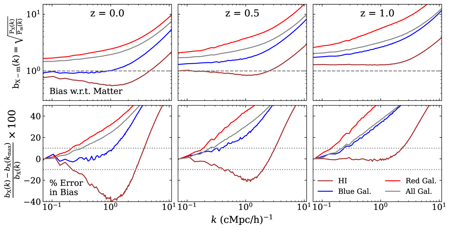
The i and galaxy biases from TNG300 are shown in the top row of Fig. 2. The bias scale-dependencies are influenced largely by two factors: the halo bias and halo occupation (Chen et al., 2021; Wang et al., 2021b). As explained in Section 3, nearly all i and galaxies reside in halos and thus reflect the shape of the halo bias. The second factor, halo occupation, modulates this behavior based on how each tracer occupies halos as a function of halo mass. Larger halos are known to cluster more strongly than smaller ones, leading to greater biases and nonlinearities both for them and the tracers that they tend to host (Sheth & Tormen, 1999; Cooray & Sheth, 2002). For example, red galaxies are known to favor older and massive halos, resulting in a greater amplitude and a sharper slope in the bias at all redshifts (Kaiser, 1984; Gao et al., 2005; Zehavi et al., 2011). Conversely, blue galaxies and i inhabit smaller, more isolated halos (Papastergis et al., 2013), resulting in smaller biases and nonlinearities (Wang et al., 2007). The remaining tracer bias in Fig. 2, all-galaxies, falls between that of blue and red galaxies, as expected from the combination of the two color subsamples.
The tendency of i and blue galaxies to occupy small halos opposes the scale-dependent contributions from the halo bias, which generates some of the unique bias shapes in Fig. 2. For example, the i bias and blue galaxy bias are constant to surprisingly small scales because the halo bias and occupation effects coincidentally offset. The occupation effect grows with time, even becoming dominant at 0.1 h cMpc-1 in the i bias at and creating the “dip” in the i bias at those scales. These i bias shapes agree with other theoretical (Pénin et al., 2018), computational (Wolz et al., 2016; Spinelli et al., 2020; Wang et al., 2021b), and observational (, Anderson et al., 2018) works on i distributions. We note however that the amplitude of the i bias can vary substantially between the different works (further discussed in Section 6.1).
The scale-dependency of each tracer bias determines the scales at which a constant bias can be assumed without inheriting significant errors, shown in the bottom row of Fig. 2. We define the “valid” scales to have errors smaller than 10% (gray dotted lines), with representing the scale at which the error crosses this threshold. The 10% threshold corresponds to of the measurement uncertainties from C22, such that roughly coincides with the scale at which differences between the scale-dependent and constant bias are no longer negligible. We note that the improved handling of systematics in C24 have already reduced these uncertainties, making the theoretical errors more impactful. More faithful comparisons require instrument-by-instrument mock observations — we address these in Section 5.3.2.
We quantify the scale-dependency of each tracer by measuring deviations from their large-scale values, assumed to be constant. The constant biases are estimated by averaging over 0.043 h cMpc-1 0.105 h cMpc-1 ( = 0.08 h cMpc-1), mitigating the impact of the small number of samples in the largest -modes. These large-scale biases and their corresponding values are given in Table 1. The bottom row of Fig. 2 shows that red galaxy bias deviates the most from its large-scale limit, while blue galaxies and i deviate the least. This result follows from the analysis of how the halo bias and occupation effects manifest in each tracer bias — namely, each effect compounds in red galaxies and offset in i and blue galaxies.
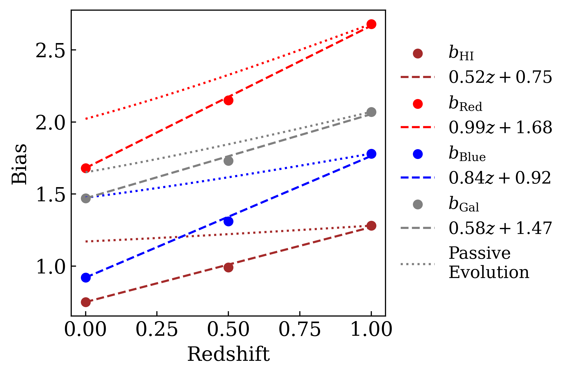
After studying the scale-dependence of the tracer biases, we now turn to their redshift evolution, which can provide insight into the role that gravity plays in tracer distributions. A population in which gravity solely governs the evolution of its distribution is called “passively evolving” with its bias relaxing toward unity:
| (14) |
Significant deviations from passive evolution suggest the influence of additional processes on the tracer’s clustering beyond gravity, such as changes in number density through mergers or satellite disruption (Bell et al., 2004; Guo et al., 2013; Skibba et al., 2014). We compare the redshift evolution of the various tracer biases to the expected passive evolution in Fig. 3. We fit a linear model to the three data points, with the slope as the only free parameter and assuming the value as the intercept.
| i | Blue Gal. | Red Gal. | All Gal. | |||||
|---|---|---|---|---|---|---|---|---|
| 0 | 0.75 | 0.22 | 0.92 | 1.15 | 1.68 | 0.23 | 1.47 | 0.35 |
| 0.5 | 0.99 | 0.41 | 1.31 | 0.32 | 2.15 | 0.20 | 1.73 | 0.26 |
| 1 | 1.28 | 2.22 | 1.78 | 0.26 | 2.68 | 0.17 | 2.07 | 0.23 |
Note. — Bias values measured from TNG300, averaged across 0.043 h cMpc-1 to reduce noise, although the averaged values agree closely with the large-scale values anyway (). (h cMpc-1) represents the scale at which these bias values deviate by from the actual scale-dependent bias. This threshold was chosen to represent when model errors become significant to measurement uncertainties from C22. The reported values should be interpreted as an optimistic estimate for this threshold.
The key conclusion from Fig. 3 is that tracers sensitive to star-formation deviate more from passive evolution than tracers independent of star-formation. This trend arises primarily from changes in how star-formation dependent tracers occupy halos. At an earlier redshift, the star-forming galaxies that occupy the most massive, clustered halos also tend to be closest to quenching. Once these galaxies quench at a later redshift, the star-forming galaxies lose their most clustered component, inducing weaker clustering on average. However, these recently-quenched galaxies join the quiescent population as their least massive, clustered members, also suppressing clustering. Therefore, galaxy quenching reduces the clustering of all tracers dependent on star-formation, like i and blue and red galaxies (for more details, see Osinga et al., 2024). The stronger role of galaxy formation physics on the distribution of i and blue galaxies at low redshifts suggests that they may be poorer tracers of the matter distribution than a star-formation independent population.
| i Blue | i Red | i Galaxy | ||||
|---|---|---|---|---|---|---|
| 0.98 | 0.35 | 0.86 | 0.17 | 0.90 | 0.17 | |
| 0.98 | 0.41 | 0.88 | 0.23 | 0.93 | 0.26 | |
| 0.98 | 0.44 | 0.87 | 0.23 | 0.95 | 0.32 | |
Note. — Large-scale correlation coefficients for i Blue, i Red, and i Galaxy and the scale at which the actual correlation coefficient value differs from the large-scale value by more than (, in h cMpc-1). The correlation coefficient values are averaged over 0.043 h cMpc-1 h cMpc-1 to reduce noise. i Blue and i Red evolve negligibly with redshift at large scales. Conversely, all correlation coefficients decrease on small scales with time, increasing the values.
We note that the biases in this section include shot noise to follow previous literature, although the shot-noise-independent definition is theoretically preferred. We compare the two bias definitions in Appendix B — we emphasize that both definitions result in the same errors and only differ in how the errors are interpreted. We also note that bias values can be sensitive to resolution, although our estimates of the model errors are robust to them (see Section 6.1 and Appendix A).
4.2 Correlation coefficients
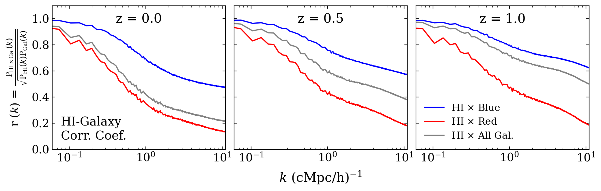
Similar to the bias studied in the previous section, the correlation coefficients presented in Fig. 4 capture complex effects on small scales that many models choose to neglect. Consequently, we adopt a similar analysis in this section, starting with the factors that shape the correlation coefficients before concluding with estimates of the scales at which an assumed constant correlation coefficient is valid.
Fig. 4 shows that i and galaxies correlate strongly on large scales, as expected since all populations trace the matter distribution. On small scales, however, stochasticity, nonlinearities, and baryonic physics decouple the tracers, reducing the correlation coefficient.
The small-scale decoupling is weakest for i and blue galaxies. Star-forming blue galaxies tend to be gas-rich and occupy the same regions of space as i, and thus strongly correlate even on small scales (Bigiel et al., 2008; Huang et al., 2012; Kauffmann et al., 2013; Papastergis et al., 2013; Hearin et al., 2016; Anderson et al., 2018). Conversely, red galaxies weakly correlate with i because they tend to inhabit gas-poor regions. i Galaxy resides between i Red and i Blue, effectively representing their weighted average. A larger fraction of galaxies are quenched at later redshifts such that i Galaxy approaches i Red with time (Nelson et al., 2018). This quenching effect does not manifest in the large-scale values of i Blue and i Red, although they are reduced on small scales. Table 2 quantifies both the redshift and color trends with estimates for the constant correlation coefficients and (definition in Section 4.1).
Since i Blue is less scale-dependent than i Red and i Galaxy, one would naïvely conclude that the i Blue cross-power spectrum is easier to model with constant bias and correlation coefficients. However, the scale-dependence of the bias opposes that of the correlation coefficient; the bias (with some exceptions, see Section 4.1) increases on small scales, while the correlation coefficient decreases. Thus, the product in the cross-power spectrum (Equation 13) may appear to be more or less scale-independent than each term individually (Appendix D).
4.3 Redshift-space distortions

| (cMpc/ | Matter | i | Blue Gal. | Red Gal. | All Gal. |
|---|---|---|---|---|---|
| 4.02 [55.0] | 2.40 [9.72] | 2.40 [22.0] | 3.59 [59.2] | 3.45 [40.2] | |
| 3.75 [9.57] | 3.12 [8.74] | 2.95 [34.5] | 2.93 [56.2] | 3.02 [20.3] | |
| 2.92 [5.87] | 2.70 [4.73] | 2.18 [14.3] | 2.11 [65.1] | 2.27 [16.0] |
Note. — Pairwise velocity dispersion (PVD) values retrieved from fits of the FoG damping term to the 2D power spectrum presented in Fig. 5. We fit down to h cMpc-1, which limits shot noise contributions. The values are calculated over the same scale regime. The galaxy populations generally have large residuals — we tested different limits and found no significant improvement in , although the PVD values change by . We attribute the poor fits to absent nonlinearities and scale-dependent effects in the FoG term, which has been found in other work (Ando et al., 2019).
Although all redshift-space distortions (RSDs) arise from line-of-sight velocities displacing the apparent positions of tracers, models often treat them as two separate contributions (see Section 3): the Kaiser and fingers-of-God (FoG) effect. A useful way to visualize these RSDs is to plot the power spectrum as a function of wavenumbers parallel () and perpendicular () to the line of sight. In this section, we analyze how RSDs manifest in the matter, i, and blue, red, and all-galaxy 2D power spectra (Fig. 5) and quantify them in Table 3.
The Kaiser effect boosts the clustering along , squeezing the isopower contours in the bottom left corner of each panel from Fig. 5 and creating horizontally-aligned ellipses. This effect’s magnitude appears similar amongst the various tracers in Fig. 5, but each Kaiser term should be inversely related to the bias of the tracer (Equation 9). We will discuss the Kaiser effect in more detail in Section 6.2 — for the remainder of this section, we focus on the FoG effect.
The FoG effect suppresses clustering at small scales, elongating the contour lines in the top left corners of each panel in Fig. 5. Amongst the galactic populations in the bottom row, the contour lines in the red galaxy panel are warped the furthest vertically, agreeing qualitatively with observations (Madgwick et al., 2003). The red galaxies’ large FoG suppression originates from their tendency to occupy massive halos with large velocity dispersions (Zehavi et al., 2011). Conversely, blue galaxies occupy smaller halos, resulting in a weaker FoG effect. The all-galaxies’ (bottom right panel) FoG strength falls between blue and red galaxies’, as expected for a combined sample. Of the two remaining populations in the top row of Fig. 5, the FoG damping in i appears to be stronger than that of matter, as seen from the more vertical contour lines in the panel’s top right corner. This agrees with conclusions from VN18, but the following discussion about Table 3 will demonstrate that this finding does not hold quantitatively.
We measure the strength of the FoG effect with the “pairwise velocity dispersion” (PVD, see Section 3). This parameter is difficult to measure directly (e.g., Loveday et al., 2018), particularly in intensity maps which do not observe point sources. Instead, the PVD is usually left as a free parameter to marginalize over (e.g., Gil-Marín et al., 2020; de Mattia et al., 2021). Following VN18, we extract the PVD (denoted ) by fitting the following equation to the 2D power spectra of the population on scales h cMpc-1:
| (15) |
where . We present the resulting PVD values in Table 3.
Most PVDs increase with time, as expected from the growth of halos bolstering their velocity dispersions. This manifests in the matter, red galaxy and all-galaxy PVDs, with the red galaxy PVDs growing rapidly enough to overtake all-galaxies by . Blue galaxies and i, however, do not evolve as expected between and 0, due to their decreasing occupation of the most massive halos which typically have the strongest dispersions (see Section 4.2). This occupation effect should also manifest between and , but the number of quenching galaxies forms a smaller proportion of the blue and i-rich population, mitigating its strength.
However, the conclusions from Fig. 5 about the relative strengths of FoG damping amongst the populations are not supported by Table 3. For example, at , red galaxies possess the smallest PVD despite their apparently large FoG suppression in Fig. 5. Out of the galaxy populations at this redshift, the all-galaxies population actually exhibits the largest PVD. Furthermore, despite the more vertical contours in i, we find that the i PVD is smaller than the matter PVD, conflicting with conclusions from VN18.
Some of the tension between Fig. 5 and Table 3 can be credited to the poor fits, which we quantify with the values in Table 3. i and matter generally maintain small values, but the galaxy populations all contain large values. To ensure that the poor fits originate from the model rather than our methodology, we tested the sensitivity of the to the scales we included in our fits ( h cMpc-1). All tests produced larger , although we found that the scale regime could change the PVD values by 0.1. PVD is a scale-dependent quantity (see Section 3.5), so the sensitivity to scale is expected. These tests suggest the poor fits stem from representing RSDs with Equation 11 for blue and red galaxy distributions, which agrees with results from other works (e.g., Hikage & Yamamoto, 2015; Orsi & Angulo, 2018).
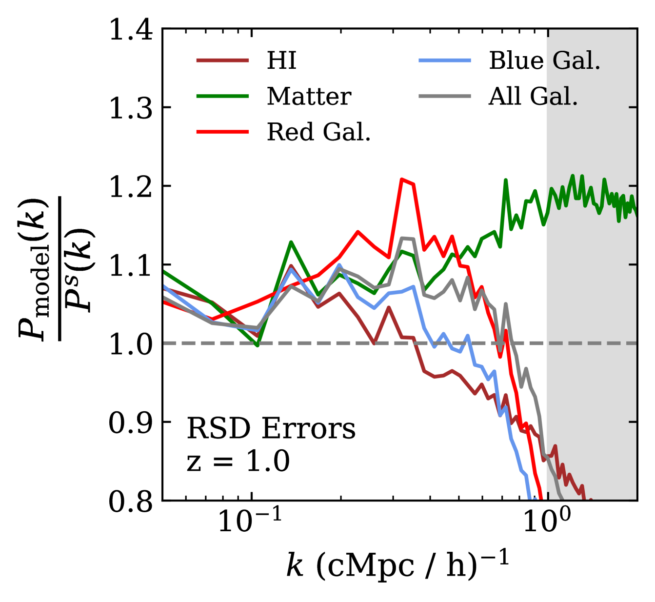
To understand how these fits shape the model errors examined in the following section, we compare the integrated 2D power spectrum model, defined as
| (16) |
to the actual redshift-space power spectrum for each population in Fig. 6 (additional redshifts provided in the online figures). Generally, we find that the integrated 2D power spectra overestimate the actual redshift-space power spectra for each population, and particularly for galaxies. i is the earliest tracer to fall below unity at h cMpc-1, although all of the galaxy tracers follow suit around h cMpc-1. We attribute this feature in the galaxy ratios to the shot noise floor that they reach around that scale, visible in their redshift-space power spectra (online figures). We limit the impact of shot noise by restricting our fits to h cMpc-1, but as previously mentioned, the fits do not improve with more or less conservative limits.
In summary, we provide the 2D power spectra for matter and each tracer in Fig. 5, and fit PVD values to them using the phenomenological model from Equation 15. However, we find that these fits misrepresent the 1D power spectrum when integrated, which may arise from the particular functional form in Equation 11 as we speculate in Section 6.2. For now, we will broadly refer to the differences shown in Fig. 6 as “RSD errors”.
5 Testing the model predictions
In Section 4, we discussed each ingredient of the general model in Equations 12-13 for i auto and cross-power spectra. The goal of this section is to understand the aggregate effect of each ingredient on the model’s performance by comparing their predictions to the simulated power spectra, seeking to answer the question “Given the i distribution in IllustrisTNG, how accurately could these models extract cosmological parameters from a perfectly measured power spectrum?” We know that any deviations between the models and simulated power spectra must arise from the combination of these ingredients failing to capture tracer clustering behavior, since each ingredient is extracted directly from the simulation. Moreover, these ingredients will be realistically further degraded by systematics and noise in observations, which are not present in our analyses. As such, we emphasize that our tests represent the best-case scenario and stated errors should be taken as lower limits. Qualitatively, the following results should be robust to cosmic variance although second-order effects could change some details (e.g., Li et al., 2014).
5.1 Hi auto power spectra
The i auto power spectrum in IllustrisTNG agrees closely with recent observations of the i auto power spectrum (P23; Osinga et al., 2024), presenting a great opportunity to leverage IllustrisTNG to test common models of large-scale i distributions. In Fig. 7, we compare four models of varying complexity by showing their ratios over the actual redshift-space i auto power spectrum from IllustrisTNG, with darker colors corresponding to more complex models (plots for additional redshifts are provided in Appendix C). The details of each prescription are described in the legend, with the background color of each row matching the corresponding power spectrum. The first two columns of the legend indicate whether or not the model assumes a constant bias or neglects the FoG effect. The third column details the equivalent equation, and the fourth column includes a shorthand that we use in the text.
On the largest scales, we expect small differences between the various models since the assumptions made by the simpler prescriptions should be appropriate (see Section 3.5). While all models converge on the largest scales, interestingly they do not converge to the actual redshift-space i auto power spectrum, overestimating it by a factor of 1.08. Noise emerging from a small number of large-scale could contribute but is unlikely to account for this difference entirely. We instead attribute the large-scale offset to the Kaiser term since all models err by the same amount regardless of bias or FoG treatment. The Kaiser term neglects nonlinearities in the matter velocity fields, which are known to emerge at h cMpc-1 (Reid & White, 2011; Jennings et al., 2011; Howlett et al., 2017). Despite the departures on the largest scales, all models remain within 10% of the actual power spectrum at h cMpc-1.
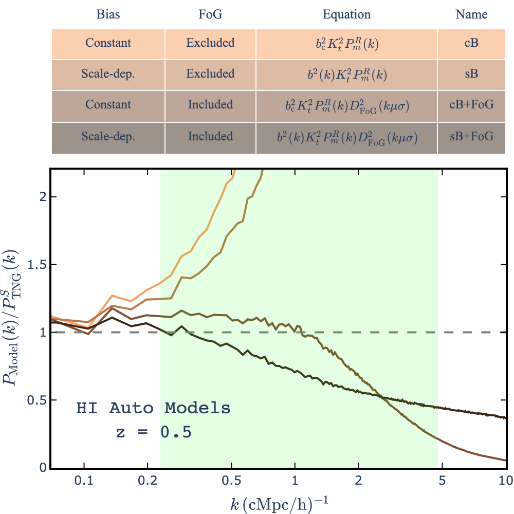
The two simplest prescriptions cross the threshold at similar scales, whether a constant (cB) or scale-dependent (sB) bias is assumed. The small difference in performance between cB and sB, despite the impractically precise description of the i bias in sB, suggests that including non-constant bias terms in i auto power spectra models would negligibly improve their performance. The errors in these models worsen to on the scales relevant to a recent observation of the i auto power spectrum, P23222We note that P23 remove modes from their analysis due to instrumentation effects, which should change model performance. As such, Fig. 7 should be interpreted as the model errors from a similar survey without this limitation. (green shaded area). Most of the error from the cB and sB models arises from neglecting the FoG term, as shown by the significant improvement in cB+FoG. Despite neglecting non-constant terms in the i bias, the cB+FoG error on observation scales remains at until h cMpc-1.
sB+FoG includes a fully scale-dependent bias and FoG term, such that RSD errors (Section 4.3) are the only remaining error sources. sB+FoG improves on cB+FoG mostly at large scales, until h cMpc-1 where their relative error inverts. cB+FoG can perform better than sB+FoG because it has two sources of error that oppose each other: the overestimated i bias and underestimated RSD effects. This phenomenon is unique to i, as the other tracers do not possess the intermediate-scale dip that allows a constant bias to overestimate the actual bias (Fig. 2). Other tracers instead always underpredict the bias, which compounds with the RSD error.
In summary, Fig. 7 shows that neglecting the FoG term, even on scales h cMpc-1, causes inaccuracies that dominate other potential error sources, like neglecting non-constant terms in the i bias. We also demonstrate that competing error sources can reduce the net error of a simple model, to the point it appears more “accurate” than a more complex model. However, even the full prescription incurs an error of on observationally relevant scales, which would significantly skew the cosmological constraints inferred from i auto power spectra.
5.2 Hi-galaxy cross-power spectra
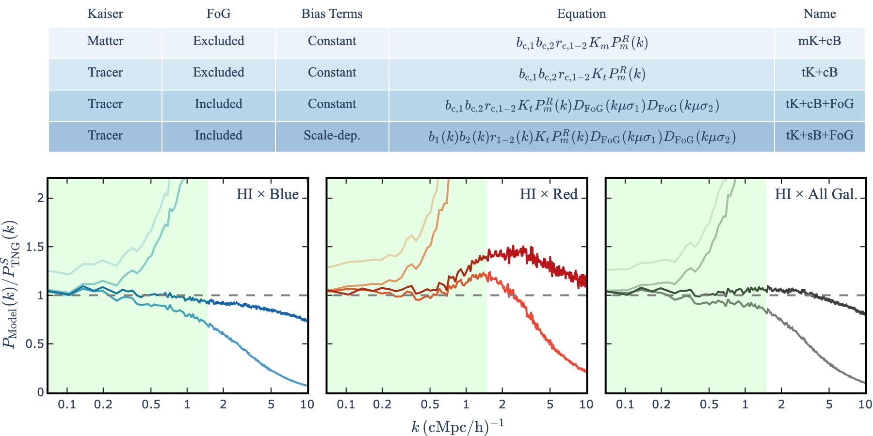
Cross-correlations between i and galaxy surveys reduce the systematics and noise present in the i auto power spectrum, at the cost of additional complexity (Equations 12-13). In this section, we investigate model errors of i-galaxy cross-power spectra in Fig. 8 at , coinciding with most observations (Chang et al., 2010; Masui et al., 2013; Wolz et al., 2022; CHIME Collaboration et al., 2023). Additional redshifts are provided in Appendix C.
Although both Fig. 7 and 8 show four models each, the models in the latter differ from the former in two ways. First, recent measurements of the i-galaxy cross-power spectrum used the matter Kaiser term (Equation 7, \al@wolz_h_2022, cunnington_h_2022, Carucci24; \al@wolz_h_2022, cunnington_h_2022, Carucci24; \al@wolz_h_2022, cunnington_h_2022, Carucci24, ), which we include in Fig. 8. As a result, the naming convention for cross-power spectra models includes a specification for the Kaiser term, whereas auto power spectra only include the type of bias and FoG terms (see legends of Fig. 7 and 8). This additional specification distinguishes the auto and cross-power spectra model shorthands. Second, we remove a cross-power spectra model that uses a scale-dependent bias but neglects the FoG effect (analogous to sB from Section 5.1) since we established in the previous section that neglecting FoG is the dominant source of error.
Out of the models in Fig. 8, we find mK+cB incurs the largest error, overpredicting the fiducial power spectra by even on the largest scales. The error is larger for populations with biases that deviate further from unity like red galaxies, such that the matter (Equation 7) and tracer (Equation 10) Kaiser terms diverge. This difference can be seen in tK+cB, which only differs from mK+cB in the Kaiser term. Since recent observations interpret their measurements with mK+cB models, the large error has important ramifications on their cosmological constraints, which we analyze in Section 5.3.
Similar to Section 5.1, we find that including an FoG term substantially enhances model performance even to the largest scales probed by TNG300, as shown in the comparison between tK+cB and tK+cB+FoG. However, the improvement manifests uniquely among the different galaxy populations due to how the non-constant bias terms and RSD errors offset each other. For example, these two error sources coincidentally cancel at for i Red but do not for i Blue or i Galaxy, despite the models for i Blue and i Galaxy incurring smaller errors in both biases and RSDs separately (see Sections 4.1 and 4.3).
In summary, Fig. 8 shows that i-galaxy cross-power spectra can be interpreted with models that include FoG on scales relevant to recent observations ( h cMpc-1), given that the acceptable error threshold is . However, a model that achieves accuracy even to the level requires exact knowledge of the full scale-dependent bias and pairwise velocity dispersion of the galaxy and i populations and a precise measurement of the cross-power spectrum without systematics.
5.3 Effect on inferred
| Paper | Galaxy Survey | Model | ||||||
|---|---|---|---|---|---|---|---|---|
| W22 | WiggleZ | 0.78 | 0.24 | mK+cB | 0.8 | 0.9 | ||
| ELG | 0.78 | 0.24 | mK+cB | 0.8 | 0.7 | |||
| LRG | 0.78 | 0.24 | mK+cB | 0.8 | 0.6 | |||
| C22 | WiggleZ | 0.43 | 0.13 | mK+cB | ||||
| C24 | WiggleZ | 0.43 | 0.13 | mK+cB | ||||
| CHIME23 | ELG | 0.96 | 1.0 | tK+cB+FoG | 1 | |||
| LRG | 0.84 | 1.0 | tK+cB+FoG | 1 | ||||
| P23 | – | 0.44 | 1.0 | sB+FoG | – | – | – | |
| – | 0.32 | 1.0 | sB+FoG | – | – | – |
Note. — The constraints from i-galaxy cross-power spectra reported in W22, C22, CHIME23, and C24, and i auto power spectra from P23. The galaxy survey indicates the cross-correlated galaxy population: WiggleZ (Blake et al., 2011) and ELG (Raichoor et al., 2020) and LRG (Ross et al., 2020) samples from the eBOSS survey. and represent the effective redshift and wavenumber (in h cMpc-1) the measurement takes place. The models listed are the closest analog to the model adopted in each work. is the quantity directly measured by W22, C22, and C24. CHIME23 reported , which we adjust to match Equation 20. These works then assume i bias () and i-galaxy correlation coefficient () values to roughly estimate from , sometimes incorporating uncertainties from the assumed values into their constraints. C24 is an extension of results from C22, so we employ the same assumed values although C24 does not directly make such assumptions. Conversely, P23 fit several parameters to their measured i auto power spectra and thus do not assume any values, but they do report values with and without priors in their fits. We adopt their values from those with priors since they agree more closely with other constraints, but we caution that the uncertainties in are likely underestimated.
In Sections 5.1-5.2, we showed that models of the form in Equations 12-13 can deviate significantly from the actual i auto and cross-power spectrum. Here, we seek to establish how these errors propagate to cosmological constraints made employing these models, using recent measurements of the cosmic abundance of i () as an example. As we will show, these analytical errors can even eclipse the stated measurement uncertainties of the constraints, suggesting that model improvements are a priority. First, we describe the procedure used to infer from i auto and cross-power spectra and compare to the directly-calculated in Fig. 9. Then, we project the differences between the inferred and actual onto recent constraints from W22, C22, CHIME23, P23, and C24 to illuminate the predicted error from determining from the i power spectra in this way. Again, we emphasize that the tests presented in this section represent the best case for these models since our results are not affected by noise or systematics and the biases, correlation coefficients, and pairwise velocity dispersions are all extracted directly from the simulation.
5.3.1 Accuracy of constraints from power spectra
Measurements of probe the state of star-formation and gas in galaxies over cosmic time and inform galaxy formation models (Wyithe, 2008; Diemer et al., 2019; Davé et al., 2020). 21cm intensity mapping experiments can determine via the amplitude of i power spectra since they directly measure brightness temperature fluctuations of i, which rescale the density fluctuations by the mean i brightness temperature (Battye et al., 2013):
| (17) |
Since , the amplitude of the i auto and cross-power spectra are proportional to and , respectively. Estimates of are obtained by fitting a chosen model to the i power spectra over a range of scales. The significance and accuracy of the constraint changes depending on the included scales due to the trade-off between model accuracy and constraining power. We follow the literature by characterizing the included scales with their average, .
We replicate the above procedure by scaling the i auto and cross-power spectra by calculated from , determined by simply summing all the i in the box. After rescaling, we then fit each of the models studied to the power spectra in Section 3. In mathematical terms, we are trying to find a such that
| (18) | |||
| (19) |
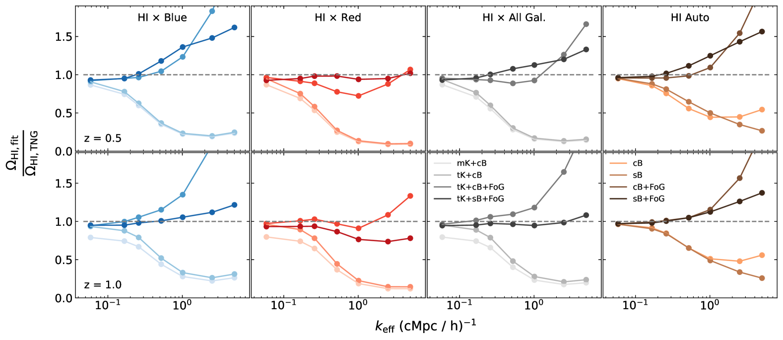
for the auto and cross-power spectra, respectively. We vary the minimum scale included in the fit to examine the small-scale trade-off between the larger errors and smaller uncertainties, expressing the inferred values as a function of . We follow previous literature to estimate the power spectra uncertainties used in the fits (Furlanetto & Lidz, 2007; Lidz et al., 2009; Park et al., 2014), removing any instrumental contributions. We compare the value determined in the fit, , to , providing the results for each model of the i auto and cross-power spectrum in Fig. 9. We exclude error bars from uncertainties in the fitted values in Fig .9 for clarity (error bars included in online figures), but we note that all uncertainties are negligible except for the value at the smallest .
Ideally, the ratios of all models should approach unity on large scales, given that the largest scales probed by TNG300 should be linear (Smith et al., 2003). The models in Fig. 9 do converge on large scales, with one exception: mK+cB, which at h cMpc-1 only reaches a ratio of about 0.8 and 0.9 for and , respectively. These errors would significantly skew the recent constraints of that resorted to this model (see Section 5.3.2). Interestingly, the remaining models also do not converge quite to unity, instead converging to and for the auto and cross-power spectra, respectively. These large-scale differences may imply that there is an absent large-scale effect in the models, although we reserve further analysis to future work with a larger-volume simulation.
This slight vertical offset between unity and the ratios serve as the largest difference between Fig. 9 and the ratios from Fig. 7 and 8. Otherwise, the errors are effectively the reciprocal of , as expected from Equation 18. Beyond this first-order effect, tends to deviate from its large-scale value at smaller than its counterpart evaluated at a similar . This trend suggests that the larger errors at have a stronger impact than the smaller ones at in the determination of .

5.3.2 Predicted impact on recent observations
We now contextualize the errors found in Section 5.3.1 by showing how recent constraints (Table 4) would change given the predicted errors from IllustrisTNG in Fig. 10. However, interpreting the observations is challenging because the i bias and i-galaxy correlation coefficient are unknown a priori and both quantities are also proportional to the power spectrum amplitude (Equations 12-13). As a result, the auto and cross-power spectra probe the degenerate quantities and , respectively. These degeneracies can be broken in the quadrupole and hexadecapole (Equation 8) in future surveys with improved signal-to-noise, but current observations of the cross-power spectrum resort to constraints of the quantity
| (20) |
taking from the galaxy survey. can be roughly estimated from by assuming values of and from theoretical predictions, which can vary amongst the different works (values given in Table 4). We replace the and estimates from observations with those from TNG300 to enable consistent comparisons in Fig. 10, but we still present the original values for completeness (open circles). We then use the estimate of the corresponding model error from IllustrisTNG at the nearest ( values from Fig. 9) to predict what the “actual” values would be (crosses) if the measurements were interpreted with a perfect model. We note that for each observation, which usually underestimates model errors since they typically grow with redshift across .
However, the i distribution in IllustrisTNG would not be perfectly measured by 21cm intensity mapping experiments due to re-gridding (Cunnington & Wolz, 2024) and the beams of the instruments themselves. In previous sections, we remained agnostic to instrument-specific effects in order to keep our results general and to focus on errors originating from models. In Fig. 10, however, we examine the impact of model errors on the constraints from specific observations. To imitate how each instrument would observe IllustrisTNG’s i distribution, we apply a Gaussian filter to the simulated redshift-space i density grid, following Wolz et al. (2017):
| (21) | ||||
| (22) |
Here, , , , and are the co-moving distance, speed of light, number of grid points along one axis, and redshifted 21cm line, respectively. represents the diameter of the dish for each radio telescope — we use 100m for Greenbank Telescope (GBT, Masui et al., 2013; Switzer et al., 2013) and 13.5m for MeerKAT (MKT, Wang et al., 2021a). We assume a constant beam size along the line of sight, as the box is at one redshift, and apply the smoothing on each two-dimensional slice perpendicular to the line-of-sight () independently.
We also adjust our model to accommodate the beam, following Ando et al. (2019):
| (23) |
where represents the angular resolution of each instrument at the redshift of interest. Overall, including the beam reduces the error estimates by a factor of 0.95 for C22, W22, and C24. We do not employ this procedure for CHIME23 or P23, as they adopt more complicated pipelines to interpret their data. We instead directly apply the error estimates from Fig. 9; the corresponding results shown in Fig. 10 should be understood as the lower limit on the magnitude of errors originating from the model333P23 adopted a halo model in their i auto power spectrum model, which requires additional assumptions on how i occupies halos. If these assumptions are valid, then sB+FoG is an appropriate equivalent (Table 4)., excluding any instrumental effects.
Fig. 10 shows that the employed models significantly bias the inferred even with respect to the stated uncertainties for each measurement. The magnitude of the error can vary with the model and redshift. For example, the mK+cB model incurs larger errors for W22 than C22 and C24 because the matter Kaiser term assumption is safer for late-time biases that approach unity (Table 1). Conversely, CHIME23 adopts a more complex model that resembles tK+cB+FoG, which somewhat mitigates the analytical error at the expense of larger uncertainties.
Overall, the revisions improve the agreement between the constraints from i-galaxy cross-power spectra and other techniques (Zwaan et al., 2005; Rao et al., 2006; Lah et al., 2007; Martin et al., 2010; Braun, 2012; Rhee et al., 2013; Hoppmann et al., 2015; Rao et al., 2017; Jones et al., 2018; Bera et al., 2019; Hu et al., 2019; Chowdhury et al., 2020). This is particularly true for the constraints from W22, while revised values from C22, CHIME23, and C24 are still consistent with the other constraints. The constraint from CHIME ELG is revised downward, although it is not shown in Fig. 10 due to its unusually large value — CHIME23 attribute this to a chance fluctuation and the prior volume effect (see their section 6.3).
Even when considering the ideal, best-case limit of these models, the revisions in Fig. 10 demonstrate that current constraints can be limited by systematics in the analysis rather than the signal-to-noise of the measurements themselves. Clearly, more sophisticated models are needed (more in Section 6.2) in order to properly realize the capabilities of future 21cm intensity mapping experiments with improved signal-to-noise.
6 Discussion
6.1 What is the impact of simulation technique on the hydrogen distribution?
| Source | Methodology | Post-Processing | (h cMpc-1) | Other Cuts () | ||
|---|---|---|---|---|---|---|
| This work | Hydro | - | 5.9 | 0.07 | - | 1.28 |
| Ando et al. (2019) | Hydro | - | 2.9 | 0.26 | - | 1.22 |
| VN18 | Hydro | - | 7.5 | 0.15 | - | 1.49 |
| Wolz et al. (2016) | N-body | SAM | ||||
| Spinelli et al. (2020) | N-body | SAM | 1.22 | |||
| Wang et al. (2021b) | N-body | SAM | 0.05 | 1.26 | ||
| Guo et al. (2023) | N-body | SAM | 0.05 | 1.10 | ||
| Spinelli et al. (2020) | N-body | SAM | 1.31 | |||
| Wang et al. (2021b) | N-body | HIHM | 0.05 | 1.48 | ||
| Sarkar et al. (2016) | N-body | HIHM | 0.065 | - | ||
| VN18 | N-body | HIHM | 7.5 | 0.15 | - | |
| Pénin et al. (2018) | Analytical | - | - | 0.01 | - | 0.82 |
| Umeh (2017) | Analytical | - | - | 0.01 | - | 0.86 |
Note. — Summary of the i bias values found in various computational and theoretical works. The values are grouped by methodology (see text for explanation) and ordered from top to bottom by increasing mass resolution (fourth column). Some works make additional mass cuts to avoid including poorly resolved structures (sixth column). (fifth column) represents the approximate scale at which the bias was measured, although the impact of this should be small since the i bias is nearly constant to very small scales in all works. Bias values averaged over different models or estimated are denoted with . We aim to establish rough trends and thus do not report statistical uncertainties arising from cosmic variance for simplicity.
In Section 5, we found that IllustrisTNG predicts that general large-scale models (Equations 12-13) introduce significant errors in cosmological constraints. However, simulated i distributions can be sensitive to the included galaxy formation physics (Park et al., 2014; Li et al., 2024; Marasco et al., 2025). This raises a key question: does IllustrisTNG’s galaxy formation model inherently yield complicated i distributions? We explore this question by comparing results from some selected computational and theoretical works in Table 5, broadly characterized by their i bias.
We examine results from three methodologies: Hydro, N-body, and Analytical. The first two, Hydro and N-body, describe simulations that differ in their handling of baryons. Hydrodynamical simulations like IllustrisTNG include baryonic physics on-the-fly, whereas N-body simulations defer baryon modeling to post-processing, typically through a i-halo mass relation (HIHM) or semi-analytic model (SAM). In the remaining methodology, Analytical, perturbation theory (Bernardeau et al., 2002) and a halo model are employed to study i distributions without a simulation.
i bias values in the first methodology, Hydro, appear to agree across different simulations at (also see figure 2 from Ando et al., 2019), although they show notable dependence on resolution. We note that our model tests are robust against these resolution effects since they are dependent on the i bias shape, rather than its precise value (Appendix A). We attribute the Hydro resolution dependence to differences in how i occupies the largest halos. VN18 found that massive halos in coarser simulations tended to contain less i than finer ones, in turn suppressing i clustering. This agrees with other works that studied the resolution dependence of star-formation in IllustrisTNG. For example, Donnari et al. (2021) found that the quenching of the massive satellites () in these massive host halos is enhanced in the coarser IllustrisTNG simulations, in turn suggesting reduced i abundance.
SAMs exhibit a similar resolution trend in their i clustering, albeit for different reasons. Instead of a reduction of i occupation in large halos, SAMs of coarser-resolution simulations possess enhanced i occupation in small halos (see figure 6 in Spinelli et al., 2020). In both SAMs and Hydro, i occupies smaller halos on average, suppressing its clustering. The i bias value also depends on the particular SAM implementation, as demonstrated by Wolz et al. (2016) and Guo et al. (2023). Identifying the particular SAM components that cause these differences is left to future work.
HIHMs, conversely, have a non-trivial dependence on resolution and the employed HIHM. The resolution dependence is clearest when comparing VN18 and Wang et al. (2021b), which adopt the same HIHM but still find i biases that differ by . Wang et al. (2021b) reasoned that the discrepancy arises because halos below their resolution threshold contribute non-negligibly to the overall i distribution. However, even at similar resolutions, Sarkar et al. (2016) and Wang et al. (2021b) find biases that differ by , implying that the i bias is also dependent on the adopted HIHM.
Comparisons among the methodologies indicate that i bias values are sensitive to secondary halo properties, such as halo age or assembly history (Gao et al., 2005). Methodologies like Hydro and SAMs that natively incorporate these assembly effects generally converge within , particularly at comparable resolutions (Ando et al., 2019). Marasco et al. (2016) found that SAMs have stronger i occupation in dense environments as compared to Hydro, which may influence the remaining differences between Hydro and SAMs. Conversely, methodologies that neglect assembly effects are either substantial outliers from Hydro and SAMs, like Analytical, or vary dramatically between implementations, like HIHM. However, in the case of HIHM, VN18 showed that its overall normalization and the fraction of i outside of halos can also contribute to this disparity in behavior.
In summary, Table 5 shows that the predicted amplitude of the i bias is dependent on the methodology and resolution. Throughout the section, we have provided some speculative reasons for these trends. Conversely, the shape of the i bias is qualitatively similar throughout the various works, which indicates that our results are robust against these effects. A deeper study that quantitatively establishes these methodology and resolution relationships is needed to develop and test more sophisticated models on realistic i distributions at .
6.2 Why is the FoG effect such a large source of error?
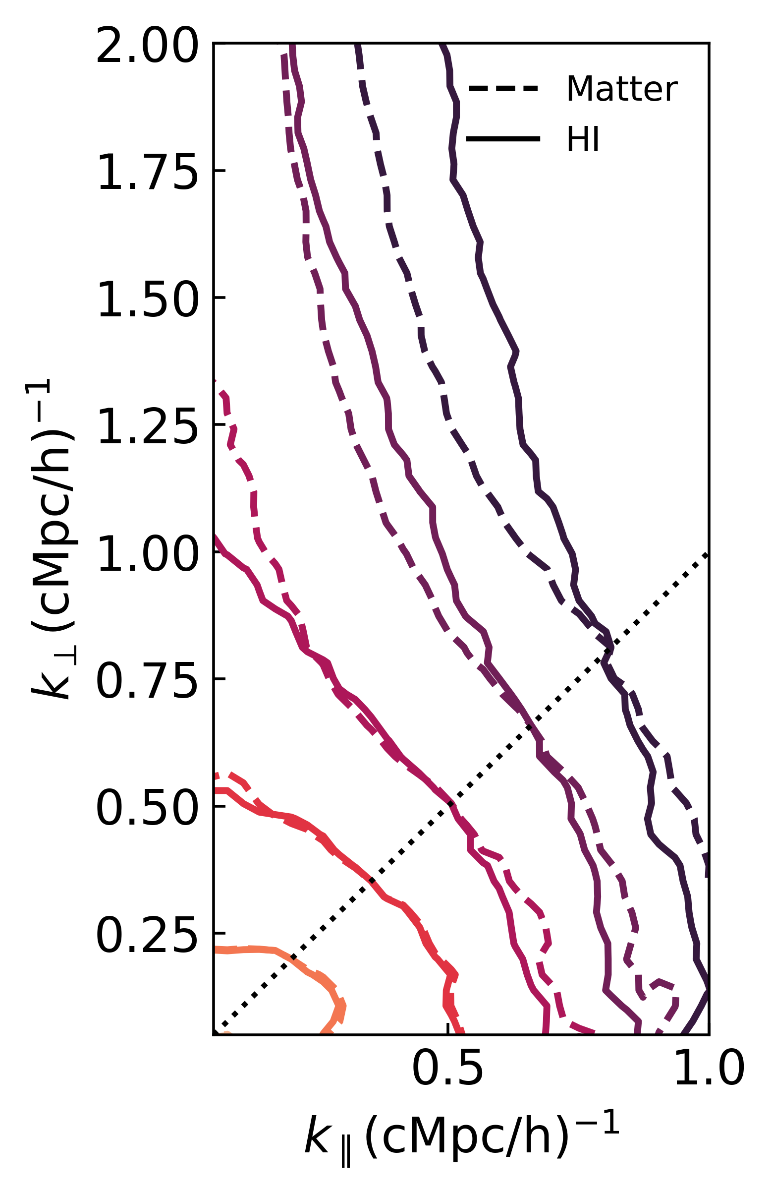
Throughout Sections 4-5, we found considerable evidence that an FoG term like Equation 11 is a poor fit to the auto power spectra, resulting in our so-called “RSD errors”. In this section, we further demonstrate with Fig. 11 that models like Equations 12-13 may insufficiently describe i RSDs, speculate on potential reasons for these issues, and conclude by proposing adjustments to these models.
We compare in Fig. 11 the relative FoG damping strength in i and matter, finding that i contains stronger damping than matter on large scales and vice versa on small scales. However, Equations 12-13 contain a single damping term whose strength is controlled by a scale-independent quantity, the pairwise velocity dispersion (PVD). Since matter possesses the larger PVD, we would expect that matter experiences stronger damping at all scales. Fig. 11 conflicts with this picture, suggesting instead that multiple RSD damping contributions are folded into the “FoG” term.
One known auxiliary damping source is the neglected nonlinear Kaiser terms in Equations 12-13, which are typically included as corrections to the matter power spectrum (Scoccimarro, 2004; Taruya et al., 2010). Ando et al. (2019) demonstrated that strictly linear models have reduced PVDs relative to models with these terms (see their figure 5). However, these models necessarily assume that nonlinearities manifest the same in i and matter (i.e., no i velocity bias), and furthermore including these nonlinearities can actually worsen model performance at h cMpc-1. Given these complications, it is uncertain if the nonlinear contributions to the Kaiser term alone can capture the trends seen in Fig. 11.
Differences in the small- and large-scale behavior of the i PVD may also give rise to the behavior in Fig. 11. The i PVD can be understood in a halo framework as contributions of three terms, each dominating at different scale regimes: inter-halo (large scales), intra-halo (intermediate), and intra-galactic (small) velocity dispersions (Slosar et al., 2006; Sarkar & Bharadwaj, 2019). The last contribution is unique to i intensity maps as compared to point-source tracers like galaxies, which would not have intra-galactic dispersions (P23; Li et al., 2024). Osinga et al. (2024) showed that the i power spectrum with and without these intra-galactic dispersions diverge at h cMpc-1 in IllustrisTNG, with the latter asymptoting to a constant shot noise floor. This comparison demonstrates that intra-galactic dispersions become important at h cMpc-1 and the real-space shot noise term is damped only by intra-galactic dispersions444Strictly speaking, shot noise only manifests on scales where random noise emerges and thus cannot be “damped” by RSDs. A more precise interpretation is that i fills a larger fraction of intra-halo spaces in redshift space, effectively lowering the shot noise floor compared to real space. Consequently, the actual redshift-space shot noise floor should resurface at smaller scales.. Given this conclusion, we propose that i power spectra be modeled phenomenologically with two separate FoG damping terms:
| (24) |
Here, symbolizes the shot noise term from the real-space i auto power spectrum. represents the i PVD, which would include all three inter-halo, intra-halo, and intra-galactic components, whereas only includes the intra-galactic dispersions. The two distinct damping terms would reproduce the behavior in Fig. 11 if , assuming that shot noise is not significant to the matter power spectrum. A thorough understanding of the distribution of the galactic i emission profiles can improve the modeling of (Li et al., 2024).
7 Conclusion
We have evaluated the performance of models of the large-scale i distribution against the hydrodynamical simulation IllustrisTNG. Specifically, we compare predictions for i auto and cross-power spectra with blue, red, and the whole galaxy population. This analysis is completed in two phases. First, we extract the model ingredients from the simulation and assessed the validity of common assumptions regarding the functional form of each term. From those ingredients, we construct model power spectra and compare them to the simulated power spectra. Based on these deviations, we predict the impact of these models on inferred constraints on the cosmic abundance of i (). Generally, we find that models, even in the best-case scenario, struggle to accurately capture i auto and cross-power spectra on scales relevant to observations, such that the model introduces errors that are comparable to current measurement uncertainties. Specifically, we conclude the following:
-
1.
The error from assuming a constant bias reaches at h cMpc-1 for i and all galaxy populations. The exceptions are the i bias and blue galaxy bias, which remain constant at level until h cMpc-1 because halo occupation effects and nonlinear clustering coincidentally cancel.
-
2.
The error from assuming a constant i-blue galaxy correlation coefficient reaches at h cMpc-1. Conversely, i-red deviates from its large-scale value by on all scales probed by IllustrisTNG ( h cMpc-1).
-
3.
Models with a linear Kaiser term and a single FoG damping term overestimate the corresponding redshift-space power spectra by at h cMpc-1 for all power spectra studied. We find that the i pairwise velocity dispersion has different large- and small-scale behavior and propose an adjustment to how RSDs are modeled (Section 6.2).
-
4.
We test two common explicit assumptions made to simplify models of tracer power spectra: neglecting the FoG term and assuming a constant bias. Of the two, neglecting FoG suppression causes the largest error in i auto and i-galaxy cross-power spectra, reaching by h cMpc-1 in both. Assuming a constant bias causes a error by h cMpc-1.
-
5.
Even with perfect knowledge of the tracer bias and RSD parameters, the tested models still deviate from the actual i auto and i-galaxy cross-power spectra by at scales relevant for observations.
-
6.
We estimate the error in recent constraints from models used to interpret recent i-galaxy cross-power spectra constraints. We find that the model errors significantly skew the obtained values by 15-30%, larger than some measurements’ statistical uncertainties. Accounting for these model errors The revisions improve agreement in values from cross-power spectra and other techniques.
These results have important ramifications for analytical treatments of i auto and cross-power spectra at low redshift. Even in the ideal scenario, where each model ingredient is measured exactly, our tested large-scale i models introduce systematic errors comparable to current statistical uncertainties in the constraints of cosmological values. The performance of these models is limited by how they model RSDs, suggesting that future analytical work should focus on improving our understanding of how RSDs manifest in tracer distributions.
However, we only studied the performance of these models using a single suite of simulations. Completing similar studies with other simulations would test how its architecture impacts the resulting tracer distributions and the performance of large-scale i models. Furthermore, we only examine how models perform in the monopole — higher-order cross-correlations between i and galaxies can provide even more constraining power, but require even more sophisticated models (e.g., Witzemann et al., 2019; Chand et al., 2024).
Acknowledgements
We would like to thank Steven Cunnington and Laura Wolz for their advice, comments, and helpful resources in replicating their work. We also thank Alkistis Pourtsidou and Yi-chao Li for their useful discussions. Research was performed in part using the compute resources and assistance of the UW-Madison Center For High Throughput Computing (CHTC) in the Department of Computer Sciences. The CHTC is supported by UW-Madison, the Advanced Computing Initiative, the Wisconsin Alumni Research Foundation, the Wisconsin Institutes for Discovery, and the National Science Foundation. We also acknowledge the University of Maryland supercomputing resources (http://hpcc.umd.edu) made available for conducting the research reported in this paper. Other software used in this work include: numpy (Harris et al., 2020), matplotlib (Hunter, 2007), seaborn (Waskom, 2021), h5py (Collette, 2013), colossus (Diemer, 2018) and pyfftw (Gomersall, 2021). This research was supported in part by the National Science Foundation under Grant numbers 2206690 and 2338388. BD furthermore acknowledges support from the Sloan Foundation.
Data Availability
Data from the figures in this publication are available upon reasonable request to the authors. The IllustrisTNG data is available at www.tng-project.org/data.
References
- Alam et al. (2021) Alam, S., Aubert, M., Avila, S., et al. 2021, Physical Review D, 103, 083533
- Anderson et al. (2018) Anderson, C. J., Luciw, N. J., Li, Y. C., et al. 2018, Monthly Notices of the Royal Astronomical Society, 476, 3382
- Ando et al. (2019) Ando, R., Nishizawa, A. J., Hasegawa, K., Shimizu, I., & Nagamine, K. 2019, Monthly Notices of the Royal Astronomical Society, 484, 5389
- Bahé et al. (2016) Bahé, Y. M., Crain, R. A., Kauffmann, G., et al. 2016, Monthly Notices of the Royal Astronomical Society, 456, 1115
- Battye et al. (2013) Battye, R. A., Browne, I. W. A., Dickinson, C., et al. 2013, Monthly Notices of the Royal Astronomical Society, 434, 1239
- Battye et al. (2004) Battye, R. A., Davies, R. D., & Weller, J. 2004, Monthly Notices of the Royal Astronomical Society, 355, 1339
- Bell et al. (2004) Bell, E. F., Wolf, C., Meisenheimer, K., et al. 2004, The Astrophysical Journal, 608, 752
- Bera et al. (2019) Bera, A., Kanekar, N., Chengalur, J. N., & Bagla, J. S. 2019, The Astrophysical Journal, 882, L7
- Bernardeau et al. (2002) Bernardeau, F., Colombi, S., Gaztanaga, E., & Scoccimarro, R. 2002, Physics Reports, 367, 1
- Bharadwaj et al. (2001) Bharadwaj, S., Nath, B. B., & Sethi, S. K. 2001, Journal of Astrophysics and Astronomy, 22, 21
- Bigiel et al. (2008) Bigiel, F., Leroy, A., Walter, F., et al. 2008, The Astronomical Journal, 136, 2846
- Blake et al. (2011) Blake, C., Brough, S., Colless, M., et al. 2011, Monthly Notices of the Royal Astronomical Society, 415, 2876
- Braun (2012) Braun, R. 2012, The Astrophysical Journal, 749, 87
- Carlson et al. (2013) Carlson, J., Reid, B., & White, M. 2013, Monthly Notices of the Royal Astronomical Society, 429, 1674
- Carucci et al. (2020) Carucci, I. P., Irfan, M. O., & Bobin, J. 2020, Monthly Notices of the Royal Astronomical Society, 499, 304
- Carucci et al. (2017) Carucci, I. P., Villaescusa-Navarro, F., & Viel, M. 2017, Journal of Cosmology and Astroparticle Physics, 2017, 001
- Carucci et al. (2024) Carucci, I. P., Bernal, J. L., Cunnington, S., et al. 2024, arXiv e-prints, arXiv:2412.06750
- Castorina & Villaescusa-Navarro (2017) Castorina, E., & Villaescusa-Navarro, F. 2017, Monthly Notices of the Royal Astronomical Society, 471, 1788
- Chan et al. (2012) Chan, K. C., Scoccimarro, R., & Sheth, R. K. 2012, Physical Review D, 85, 083509
- Chand et al. (2024) Chand, E., Banerjee, A., Foreman, S., & Villaescusa-Navarro, F. 2024, arXiv e-prints, arXiv:2410.21225
- Chang et al. (2010) Chang, T.-C., Pen, U.-L., Bandura, K., & Peterson, J. B. 2010, Nature, 466, 463
- Chen et al. (2021) Chen, Z., Wolz, L., Spinelli, M., & Murray, S. G. 2021, Monthly Notices of the Royal Astronomical Society, 502, 5259
- CHIME Collaboration et al. (2023) CHIME Collaboration, Amiri, M., Bandura, K., et al. 2023, ApJ, 947, 16
- Chisari et al. (2019) Chisari, N. E., Alonso, D., Krause, E., et al. 2019, The Astrophysical Journal Supplement Series, 242, 2
- Chowdhury et al. (2020) Chowdhury, A., Kanekar, N., Chengalur, J. N., Sethi, S., & Dwarakanath, K. S. 2020, Nature, 586, 369
- Cole et al. (2005) Cole, S., Percival, W. J., Peacock, J. A., et al. 2005, Monthly Notices of the Royal Astronomical Society, 362, 505
- Collette (2013) Collette, A. 2013, Python and HDF5 (O’Reilly Media)
- Cooray & Sheth (2002) Cooray, A., & Sheth, R. 2002, Physics Reports, 372, 1
- Cunnington & Wolz (2024) Cunnington, S., & Wolz, L. 2024, Monthly Notices of the Royal Astronomical Society, 528, 5586
- Cunnington et al. (2019) Cunnington, S., Wolz, L., Pourtsidou, A., & Bacon, D. 2019, Monthly Notices of the Royal Astronomical Society, 488, 5452
- Cunnington et al. (2022) Cunnington, S., Li, Y., Santos, M. G., et al. 2022, Monthly Notices of the Royal Astronomical Society, 518, 6262
- Davis et al. (1985) Davis, M., Efstathiou, G., Frenk, C. S., & White, S. D. M. 1985, The Astrophysical Journal, 292, 371
- Davé et al. (2020) Davé, R., Crain, R. A., Stevens, A. R. H., et al. 2020, Monthly Notices of the Royal Astronomical Society, 497, 146
- Davé et al. (2013) Davé, R., Katz, N., Oppenheimer, B. D., Kollmeier, J. A., & Weinberg, D. H. 2013, Monthly Notices of the Royal Astronomical Society, 434, 2645
- DESI Collaboration et al. (2024) DESI Collaboration, Adame, A. G., Aguilar, J., et al. 2024, arXiv e-prints, arXiv:2404.03000
- DESI Collaboration et al. (2025) —. 2025, J. Cosmology Astropart. Phys, 2025, 021
- Desjacques et al. (2010) Desjacques, V., Crocce, M., Scoccimarro, R., & Sheth, R. K. 2010, Physical Review D, 82, 103529
- de Mattia et al. (2021) de Mattia, A., Ruhlmann-Kleider, V., Raichoor, A., et al. 2021, Monthly Notices of the Royal Astronomical Society, 501, 5616
- Diemer (2018) Diemer, B. 2018, ApJS, 239, 35
- Diemer et al. (2019) Diemer, B., Stevens, A. R. H., Lagos, C. d. P., et al. 2019, Monthly Notices of the Royal Astronomical Society, 487, 1529
- Dodelson & Schmidt (2020) Dodelson, S., & Schmidt, F. 2020, Modern Cosmology, publication Title: Modern Cosmology ADS Bibcode: 2020moco.book…..D
- Donnari et al. (2019) Donnari, M., Pillepich, A., Nelson, D., et al. 2019, Monthly Notices of the Royal Astronomical Society, 485, 4817
- Donnari et al. (2021) Donnari, M., Pillepich, A., Joshi, G. D., et al. 2021, Monthly Notices of the Royal Astronomical Society, 500, 4004
- Eisenstein et al. (2005) Eisenstein, D. J., Zehavi, I., Hogg, D. W., et al. 2005, The Astrophysical Journal, 633, 560
- Fry (1996) Fry, J. N. 1996, The Astrophysical Journal, 461, L65
- Furlanetto & Lidz (2007) Furlanetto, S. R., & Lidz, A. 2007, The Astrophysical Journal, 660, 1030
- Gao et al. (2005) Gao, L., Springel, V., & White, S. D. M. 2005, Monthly Notices of the Royal Astronomical Society, 363, L66
- Gebek et al. (2023) Gebek, A., Baes, M., Diemer, B., et al. 2023, Monthly Notices of the Royal Astronomical Society, 521, 5645
- Gebek et al. (2025) Gebek, A., Diemer, B., Martorano, M., et al. 2025, arXiv e-prints, arXiv:2501.12008
- Gil-Marín et al. (2020) Gil-Marín, H., Bautista, J. E., Paviot, R., et al. 2020, Monthly Notices of the Royal Astronomical Society, 498, 2492
- Gomersall (2021) Gomersall, H. 2021, Astrophysics Source Code Library, ascl
- Guo et al. (2023) Guo, H., Wang, J., Jones, M. G., & Behroozi, P. 2023, The Astrophysical Journal, 955, 57
- Guo et al. (2013) Guo, H., Zehavi, I., Zheng, Z., et al. 2013, The Astrophysical Journal, 767, 122
- Harris et al. (2020) Harris, C. R., Millman, K. J., van der Walt, S. J., et al. 2020, Nature, 585, 357
- Hearin et al. (2016) Hearin, A. P., Behroozi, P. S., & van den Bosch, F. C. 2016, Monthly Notices of the Royal Astronomical Society, 461, 2135
- Hikage & Yamamoto (2015) Hikage, C., & Yamamoto, K. 2015, Monthly Notices of the Royal Astronomical Society: Letters, 455, L77
- Hoppmann et al. (2015) Hoppmann, L., Staveley-Smith, L., Freudling, W., et al. 2015, Monthly Notices of the Royal Astronomical Society, 452, 3726
- Howlett et al. (2017) Howlett, C., Staveley-Smith, L., & Blake, C. 2017, Monthly Notices of the Royal Astronomical Society, 464, 2517
- Hu et al. (2019) Hu, W., Hoppmann, L., Staveley-Smith, L., et al. 2019, Monthly Notices of the Royal Astronomical Society, 489, 1619
- Huang et al. (2012) Huang, S., Haynes, M. P., Giovanelli, R., & Brinchmann, J. 2012, The Astrophysical Journal, 756, 113
- Hunter (2007) Hunter, J. D. 2007, Computing in Science and Engineering, 9, 90
- Jackson (1972) Jackson, J. C. 1972, Monthly Notices of the Royal Astronomical Society, 156, 1P
- Jenkins et al. (1998) Jenkins, A., Frenk, C. S., Pearce, F. R., et al. 1998, The Astrophysical Journal, 499, 20
- Jennings et al. (2015) Jennings, E., Baugh, C. M., & Hatt, D. 2015, Monthly Notices of the Royal Astronomical Society, 446, 793
- Jennings et al. (2011) Jennings, E., Baugh, C. M., & Pascoli, S. 2011, Monthly Notices of the Royal Astronomical Society, 410, 2081
- Jeong & Komatsu (2009) Jeong, D., & Komatsu, E. 2009, The Astrophysical Journal, 691, 569
- Jones et al. (2018) Jones, M. G., Haynes, M. P., Giovanelli, R., & Moorman, C. 2018, Monthly Notices of the Royal Astronomical Society, 477, 2
- Jullo et al. (2012) Jullo, E., Rhodes, J., Kiessling, A., et al. 2012, The Astrophysical Journal, 750, 37
- Kaiser (1984) Kaiser, N. 1984, The Astrophysical Journal, 284, L9
- Kaiser (1987) —. 1987, Monthly Notices of the Royal Astronomical Society, 227, 1
- Kauffmann et al. (2013) Kauffmann, G., Li, C., Zhang, W., & Weinmann, S. 2013, Monthly Notices of the Royal Astronomical Society, 430, 1447
- Krause & Eifler (2017) Krause, E., & Eifler, T. 2017, Monthly Notices of the Royal Astronomical Society, 470, 2100
- Lah et al. (2007) Lah, P., Chengalur, J. N., Briggs, F. H., et al. 2007, Monthly Notices of the Royal Astronomical Society, 376, 1357
- Leo et al. (2020) Leo, M., Theuns, T., Baugh, C. M., Li, B., & Pascoli, S. 2020, Journal of Cosmology and Astroparticle Physics, 2020, 004
- Lewis & Challinor (2011) Lewis, A., & Challinor, A. 2011, Astrophysics Source Code Library, ascl:1102.026
- Lewis et al. (2000) Lewis, A., Challinor, A., & Lasenby, A. 2000, The Astrophysical Journal, 538, 473
- Li et al. (2024) Li, X., Li, C., & Mo, H. 2024, arXiv e-prints, arXiv:2411.07977
- Li et al. (2014) Li, Y., Hu, W., & Takada, M. 2014, Physical Review D, 89, 083519
- Li et al. (2024) Li, Z., Wolz, L., Guo, H., Cunnington, S., & Mao, Y. 2024, Monthly Notices of the Royal Astronomical Society, 534, 1801
- Lidz et al. (2009) Lidz, A., Zahn, O., Furlanetto, S. R., et al. 2009, The Astrophysical Journal, 690, 252
- Loveday et al. (2018) Loveday, J., Christodoulou, L., Norberg, P., et al. 2018, Monthly Notices of the Royal Astronomical Society, 474, 3435
- Madgwick et al. (2003) Madgwick, D. S., Hawkins, E., Lahav, O., et al. 2003, Monthly Notices of the Royal Astronomical Society, 344, 847
- Marasco et al. (2016) Marasco, A., Crain, R. A., Schaye, J., et al. 2016, Monthly Notices of the Royal Astronomical Society, 461, 2630
- Marasco et al. (2025) Marasco, A., de Blok, W. J. G., Maccagni, F. M., et al. 2025, arXiv e-prints, arXiv:2503.03818
- Marinacci et al. (2018) Marinacci, F., Vogelsberger, M., Pakmor, R., et al. 2018, Monthly Notices of the Royal Astronomical Society, Volume 480, Issue 4, p.5113-5139, 480, 5113
- Martin et al. (2010) Martin, A. M., Papastergis, E., Giovanelli, R., et al. 2010, The Astrophysical Journal, 723, 1359
- Masui et al. (2013) Masui, K. W., Switzer, E. R., Banavar, N., et al. 2013, The Astrophysical Journal, 763, L20
- Matteo et al. (2002) Matteo, T. D., Perna, R., Abel, T., & Rees, M. J. 2002, The Astrophysical Journal, 564, 576
- McDonald & Roy (2009) McDonald, P., & Roy, A. 2009, Journal of Cosmology and Astroparticle Physics, 2009, 020
- MeerKLASS Collaboration et al. (2024) MeerKLASS Collaboration, Barberi-Squarotti, M., Bernal, J. L., et al. 2024, arXiv e-prints, arXiv:2407.21626
- Miller et al. (2002) Miller, C. J., Nichol, R. C., & Chen, X. 2002, The Astrophysical Journal, 579, 483
- Naiman et al. (2018) Naiman, J. P., Pillepich, A., Springel, V., et al. 2018, Monthly Notices of the Royal Astronomical Society, 477, 1206
- Nelson et al. (2018) Nelson, D., Pillepich, A., Springel, V., et al. 2018, Monthly Notices of the Royal Astronomical Society, 475, 624
- Nelson et al. (2019) Nelson, D., Springel, V., Pillepich, A., et al. 2019, Computational Astrophysics and Cosmology, 6, 2
- Nishimichi (2012) Nishimichi, T. 2012, Journal of Cosmology and Astroparticle Physics, 2012, 037
- Nishizawa et al. (2013) Nishizawa, A. J., Takada, M., & Nishimichi, T. 2013, Monthly Notices of the Royal Astronomical Society, 433, 209
- Orsi & Angulo (2018) Orsi, Á. A., & Angulo, R. E. 2018, Monthly Notices of the Royal Astronomical Society, 475, 2530
- Osinga et al. (2024) Osinga, C. K., Diemer, B., Villaescusa-Navarro, F., D’Onghia, E., & Timbie, P. 2024, Monthly Notices of the Royal Astronomical Society, 531, 450
- Padmanabhan et al. (2023) Padmanabhan, H., Maartens, R., Umeh, O., & Camera, S. 2023, arXiv e-prints, arXiv:2305.09720
- Papastergis et al. (2013) Papastergis, E., Giovanelli, R., Haynes, M. P., Rodríguez-Puebla, A., & Jones, M. G. 2013, The Astrophysical Journal, 776, 43
- Paranjape et al. (2013) Paranjape, A., Sefusatti, E., Chan, K. C., et al. 2013, Monthly Notices of the Royal Astronomical Society, 436, 449
- Park et al. (1994) Park, C., Vogeley, M. S., Geller, M. J., & Huchra, J. P. 1994, The Astrophysical Journal, 431, 569
- Park et al. (2014) Park, J., Kim, H.-S., Wyithe, J. S. B., & Lacey, C. G. 2014, Monthly Notices of the Royal Astronomical Society, 438, 2474
- Paul et al. (2023) Paul, S., Santos, M. G., Chen, Z., & Wolz, L. 2023, arXiv e-prints, arXiv:2301.11943
- Peacock & Dodds (1994) Peacock, J. A., & Dodds, S. J. 1994, Monthly Notices of the Royal Astronomical Society, 267, 1020
- Percival & White (2009) Percival, W. J., & White, M. 2009, Monthly Notices of the Royal Astronomical Society, 393, 297
- Pillepich et al. (2018a) Pillepich, A., Nelson, D., Hernquist, L., et al. 2018a, Monthly Notices of the Royal Astronomical Society, 475, 648
- Pillepich et al. (2018b) Pillepich, A., Springel, V., Nelson, D., et al. 2018b, Monthly Notices of the Royal Astronomical Society, 473, 4077
- Planck Collaboration et al. (2016) Planck Collaboration, Ade, P. A. R., Aghanim, N., et al. 2016, Astronomy & Astrophysics, 594, A13
- Podczerwinski & Timbie (2024) Podczerwinski, J., & Timbie, P. T. 2024, Monthly Notices of the Royal Astronomical Society, 527, 8382
- Pénin et al. (2018) Pénin, A., Umeh, O., & Santos, M. G. 2018, Monthly Notices of the Royal Astronomical Society, 473, 4297
- Raichoor et al. (2020) Raichoor, A., Eisenstein, D. J., Karim, T., et al. 2020, Research Notes of the American Astronomical Society, 4, 180
- Rao et al. (2006) Rao, S. M., Turnshek, D. A., & Nestor, D. B. 2006, The Astrophysical Journal, 636, 610
- Rao et al. (2017) Rao, S. M., Turnshek, D. A., Sardane, G. M., & Monier, E. M. 2017, Monthly Notices of the Royal Astronomical Society, 471, 3428
- Reddick et al. (2014) Reddick, R. M., Tinker, J. L., Wechsler, R. H., & Lu, Y. 2014, The Astrophysical Journal, 783, 118
- Reid & White (2011) Reid, B. A., & White, M. 2011, Monthly Notices of the Royal Astronomical Society, 417, 1913
- Rhee et al. (2013) Rhee, J., Zwaan, M. A., Briggs, F. H., et al. 2013, Monthly Notices of the Royal Astronomical Society, 435, 2693
- Robertson et al. (2024) Robertson, A., Huff, E., Markovič, K., & Li, B. 2024, Monthly Notices of the Royal Astronomical Society, 533, 4081
- Ross et al. (2020) Ross, A. J., Bautista, J., Tojeiro, R., et al. 2020, Monthly Notices of the Royal Astronomical Society, 498, 2354
- Saito et al. (2014) Saito, S., Baldauf, T., Vlah, Z., et al. 2014, Physical Review D, 90, 123522
- Sarkar & Bharadwaj (2018) Sarkar, D., & Bharadwaj, S. 2018, Monthly Notices of the Royal Astronomical Society, 476, 96
- Sarkar & Bharadwaj (2019) —. 2019, Monthly Notices of the Royal Astronomical Society, 487, 5666
- Sarkar et al. (2016) Sarkar, D., Bharadwaj, S., & Anathpindika, S. 2016, Monthly Notices of the Royal Astronomical Society, 460, 4310
- Scoccimarro (2004) Scoccimarro, R. 2004, Physical Review D, 70, 083007
- Seljak & Warren (2004) Seljak, U., & Warren, M. S. 2004, Monthly Notices of the Royal Astronomical Society, 355, 129
- Sheth et al. (2001) Sheth, R. K., Hui, L., Diaferio, A., & Scoccimarro, R. 2001, Monthly Notices of the Royal Astronomical Society, 325, 1288
- Sheth & Tormen (1999) Sheth, R. K., & Tormen, G. 1999, Monthly Notices of the Royal Astronomical Society, 308, 119
- Skibba et al. (2014) Skibba, R. A., Smith, M. S. M., Coil, A. L., et al. 2014, The Astrophysical Journal, 784, 128
- Slosar et al. (2006) Slosar, A., Seljak, U., & Tasitsiomi, A. 2006, Monthly Notices of the Royal Astronomical Society, 366, 1455
- Smith & Angulo (2019) Smith, R. E., & Angulo, R. E. 2019, Monthly Notices of the Royal Astronomical Society, 486, 1448
- Smith et al. (2003) Smith, R. E., Peacock, J. A., Jenkins, A., et al. 2003, Monthly Notices of the Royal Astronomical Society, 341, 1311
- Somerville et al. (2004) Somerville, R. S., Lee, K., Ferguson, H. C., et al. 2004, The Astrophysical Journal, 600, L171
- Spinelli et al. (2020) Spinelli, M., Zoldan, A., De Lucia, G., Xie, L., & Viel, M. 2020, Monthly Notices of the Royal Astronomical Society, 493, 5434
- Springel (2010) Springel, V. 2010, Monthly Notices of the Royal Astronomical Society, 401, 791
- Springel et al. (2001) Springel, V., White, S. D. M., Tormen, G., & Kauffmann, G. 2001, Monthly Notices of the Royal Astronomical Society, 328, 726
- Springel et al. (2018) Springel, V., Pakmor, R., Pillepich, A., et al. 2018, Monthly Notices of the Royal Astronomical Society, 475, 676
- Stevens et al. (2019) Stevens, A. R. H., Diemer, B., Lagos, C. D. P., et al. 2019, Monthly Notices of the Royal Astronomical Society, 483, 5334
- Stoughton et al. (2002) Stoughton, C., Lupton, R. H., Bernardi, M., et al. 2002, The Astronomical Journal, 123, 485
- Switzer et al. (2013) Switzer, E. R., Masui, K. W., Bandura, K., et al. 2013, Monthly Notices of the Royal Astronomical Society, 434, L46
- Takahashi et al. (2012) Takahashi, R., Sato, M., Nishimichi, T., Taruya, A., & Oguri, M. 2012, The Astrophysical Journal, 761, 152
- Taruya et al. (2010) Taruya, A., Nishimichi, T., & Saito, S. 2010, Physical Review D, 82, 063522
- Tegmark et al. (2002) Tegmark, M., Hamilton, A. J. S., & Xu, Y. 2002, Monthly Notices of the Royal Astronomical Society, 335, 887
- Umeh (2017) Umeh, O. 2017, Journal of Cosmology and Astroparticle Physics, 2017, 005
- Umeh et al. (2016) Umeh, O., Maartens, R., & Santos, M. 2016, Journal of Cosmology and Astroparticle Physics, 2016, 061
- van Daalen et al. (2011) van Daalen, M. P., Schaye, J., Booth, C. M., & Dalla Vecchia, C. 2011, Monthly Notices of the Royal Astronomical Society, 415, 3649
- Villaescusa-Navarro (2024) Villaescusa-Navarro, F. 2024, Astrophysics Source Code Library, ascl:2403.012
- Villaescusa-Navarro et al. (2018) Villaescusa-Navarro, F., Genel, S., Castorina, E., et al. 2018, The Astrophysical Journal, 866, 135
- Vlah et al. (2015) Vlah, Z., Seljak, U., & Baldauf, T. 2015, Physical Review D, 91, 023508
- Vogelsberger et al. (2013) Vogelsberger, M., Genel, S., Sijacki, D., et al. 2013, Monthly Notices of the Royal Astronomical Society, 436, 3031
- Wang et al. (2021a) Wang, J., Santos, M. G., Bull, P., et al. 2021a, Monthly Notices of the Royal Astronomical Society, 505, 3698
- Wang et al. (2007) Wang, Y., Yang, X., Mo, H. J., & van den Bosch, F. C. 2007, The Astrophysical Journal, 664, 608
- Wang et al. (2021b) Wang, Z., Chen, Y., Mao, Y., et al. 2021b, The Astrophysical Journal, 907, 4
- Waskom (2021) Waskom, M. 2021, The Journal of Open Source Software, 6, 3021
- Weinberger et al. (2018) Weinberger, R., Springel, V., Pakmor, R., et al. 2018, Monthly Notices of the Royal Astronomical Society, 479, 4056
- White & Rees (1978) White, S. D. M., & Rees, M. J. 1978, Monthly Notices of the Royal Astronomical Society, 183, 341
- Witzemann et al. (2019) Witzemann, A., Alonso, D., Fonseca, J., & Santos, M. G. 2019, Monthly Notices of the Royal Astronomical Society, 485, 5519
- Wolz et al. (2017) Wolz, L., Blake, C., & Wyithe, J. S. B. 2017, Monthly Notices of the Royal Astronomical Society, 470, 3220
- Wolz et al. (2016) Wolz, L., Tonini, C., Blake, C., & Wyithe, J. S. B. 2016, Monthly Notices of the Royal Astronomical Society, 458, 3399
- Wolz et al. (2022) Wolz, L., Pourtsidou, A., Masui, K. W., et al. 2022, Monthly Notices of the Royal Astronomical Society, 510, 3495
- Wyithe (2008) Wyithe, J. S. B. 2008, Monthly Notices of the Royal Astronomical Society, 388, 1889
- Zehavi et al. (2004) Zehavi, I., Weinberg, D. H., Zheng, Z., et al. 2004, The Astrophysical Journal, 608, 16
- Zehavi et al. (2011) Zehavi, I., Zheng, Z., Weinberg, D. H., et al. 2011, The Astrophysical Journal, 736, 59
- Zhang et al. (2020) Zhang, J., Costa, A. A., Wang, B., et al. 2020, The Astrophysical Journal, 895, 34
- Zheng et al. (2007) Zheng, Z., Coil, A. L., & Zehavi, I. 2007, The Astrophysical Journal, 667, 760
- Zwaan et al. (2005) Zwaan, M. A., Meyer, M. J., Staveley-Smith, L., & Webster, R. L. 2005, Monthly Notices of the Royal Astronomical Society, 359, L30
Appendix A Resolution Effects
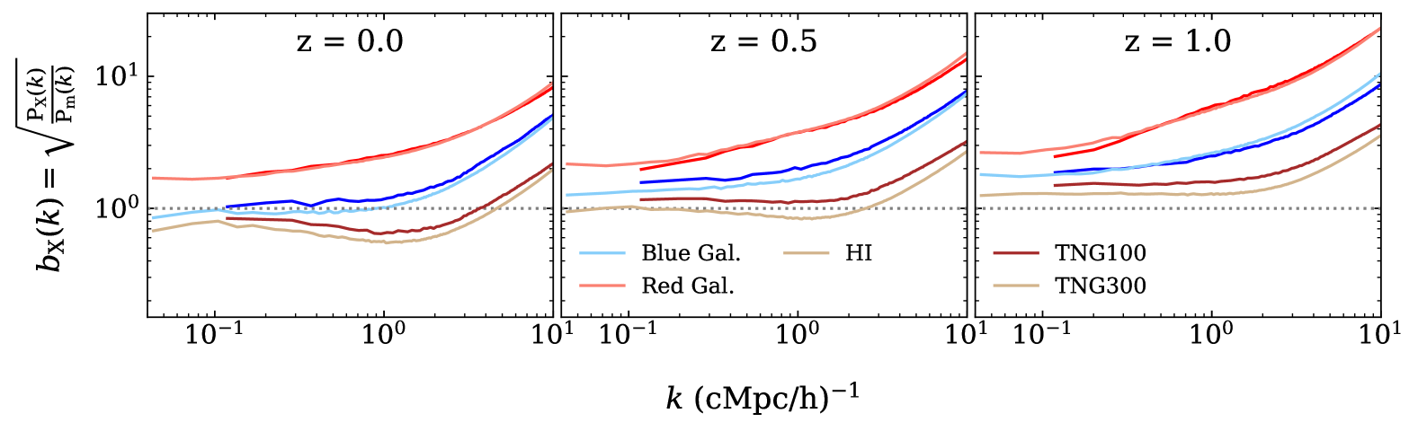
We study the resolution dependence of our results in Fig. 12 by comparing the i, blue, and red galaxy biases from TNG100 and TNG300, which have resolutions that differ by approximately an order of magnitude (Nelson et al., 2019). We find that red galaxy bias is nearly identical between the two resolutions within overlapping scales, and the blue galaxy bias converges for . At later redshifts, the blue galaxy bias has a slight vertical offset, similar to the i bias at all redshifts. The different behavior between the various tracers is expected (Section 6.1) as the blue or i-rich galaxies tend to have masses closer to the resolution limit than red galaxies, particularly at late redshifts (Villaescusa-Navarro et al., 2018; Nelson et al., 2018). Furthermore, star-formation rates are generally enhanced with better resolution, leading to less i overall (Davé et al., 2013).
Both the correlation coefficients and pairwise velocity dispersions (PVD) are also impacted significantly by resolution. The effects on the correlation coefficient can be inferred from Fig. 12 — the downward shift of the i bias implies a decrease in the i auto power spectrum, which causes all i-galaxy correlation coefficients to shift down as well (online figures). Similarly, all PVDs are expected to be dependent on resolution due to changing satellite fractions altering how virialized motions manifest in redshift space (Slosar et al., 2006). Given these resolution effects, we cannot conclude that the bias, correlation coefficient, and PVD values presented in Section 4 are converged with resolution.
However, our conclusions about model performance in Section 5 are independent of resolution effects. The precise values of the large-scale bias and correlation coefficient do not impact model error estimates, since they are removed in the ratios. Tracer RSDs can change at different mass resolutions due to how they sample the large-scale velocity field (Jennings et al., 2015; Robertson et al., 2024), but we find similar RSD errors in TNG100 VN18.
Appendix B Shot Noise
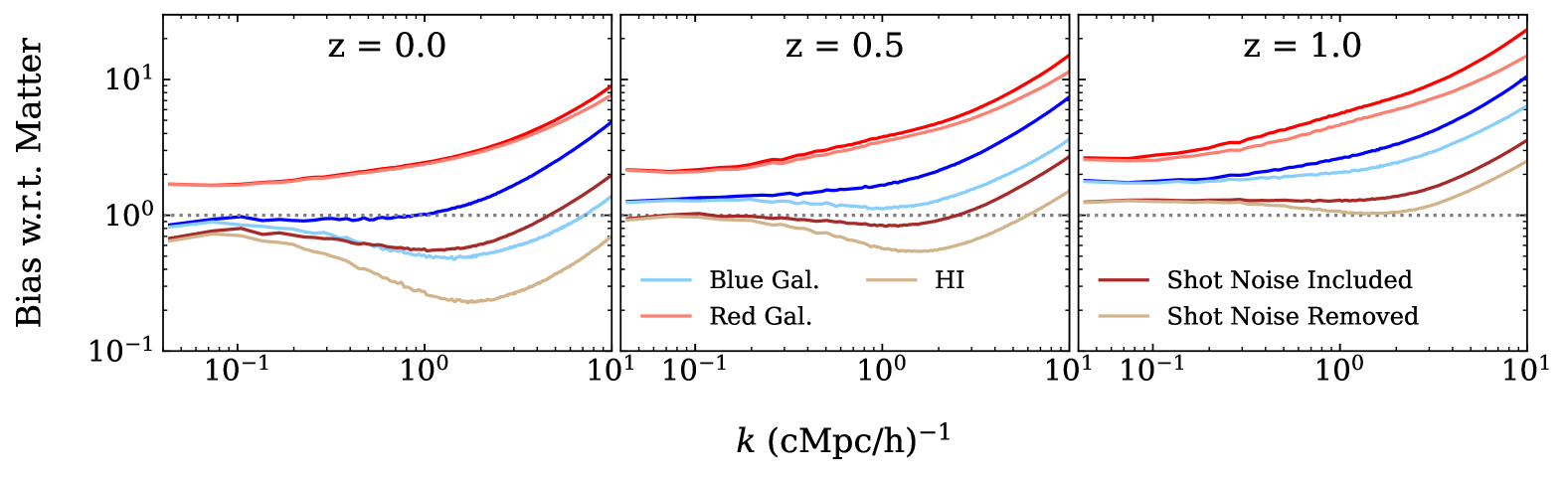
Shot noise arises in power spectra due to the discrete sampling of a continuous density field. Generally, this term is thought to be negligible on large scales but can be significant on small scales (Castorina & Villaescusa-Navarro, 2017). We establish the role of shot noise in our results by first outlining its expected behavior and then comparing bias definitions with and without shot noise in Fig. 13.
Shot noise is inversely proportional to the sample size, like where is the sample number density. For this work, however, we use mass-weighted power spectra which has a different expression for the shot noise contribution:
| (B1) |
Here, is the volume and is the mass of the th source, which in our case would be an i mass element or a galaxy. If the shot noise is purely Poisson, then is scale-independent, although can become slightly scale-dependent via residual correlations on the smallest scales (Chen et al., 2021).
Instead of folding the shot noise term into the bias like in Equation 2, we can separate the two terms with an alternative bias definition:
| (B2) |
for some tracer . With this new bias definition, the relationship between the auto power spectra of matter and tracer becomes
| (B3) |
We note that our fiducial models (Equations 12-13) and models like Equation B3 fundamentally include the same components, but attribute the shot noise to different terms. Consequently, our tests of the models using scale-dependent biases remain the same regardless of bias definition, although our analysis of the errors associated with the bias term change. We compare our fiducial bias definition to the bias from Equation B2 in Fig. 13 and re-interpret the errors linked to the bias in the context of this alternative bias definition.
All biases shown in Fig. 13 receive negligible shot noise contributions on the largest scales, although shot noise plays a larger role in blue galaxies and i than red galaxies. We attribute this to the larger sample size and stronger clustering of red galaxies, both of which diminish the significance of shot noise such that . At earlier redshifts, the red-galaxy shot noise is larger because there are fewer red galaxies. As more galaxies quench at later redshifts, the red population grows, suppressing shot noise. Conversely, the blue galaxy and i abundance decreases, strengthening shot noise.
If we were to exclude the shot noise from the bias using two distinct terms as in Equation B3, we would attribute more error to the bias term. The shot noise mitigates the scale-dependence of the bias such that assuming a constant bias appears better in Section 4.1 than it would with the alternative definition without the shot noise. This conclusion further illustrates that our results represent the best-case error estimates.
Appendix C Redshift Evolution
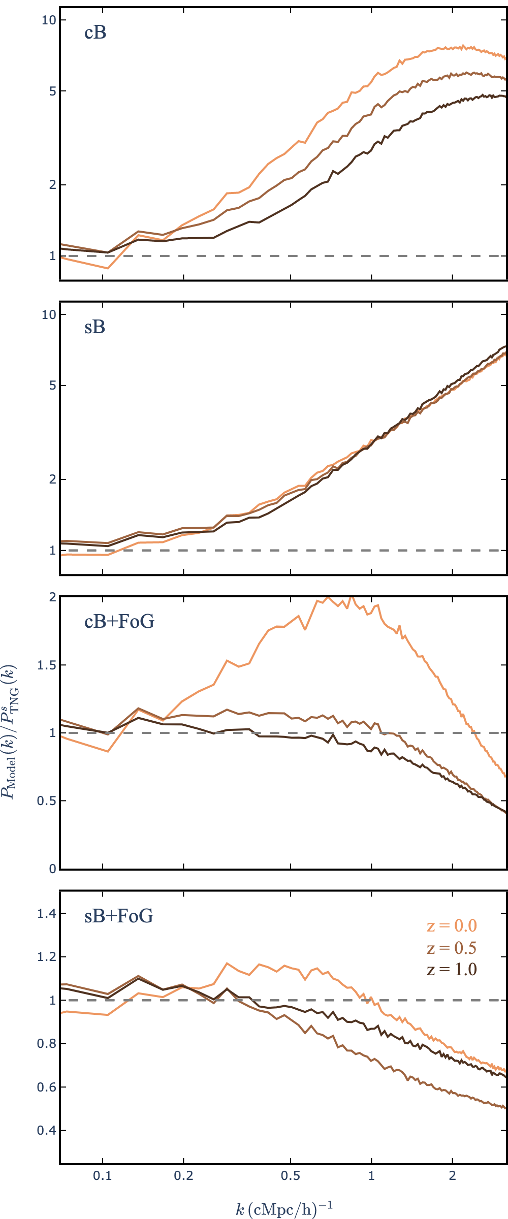
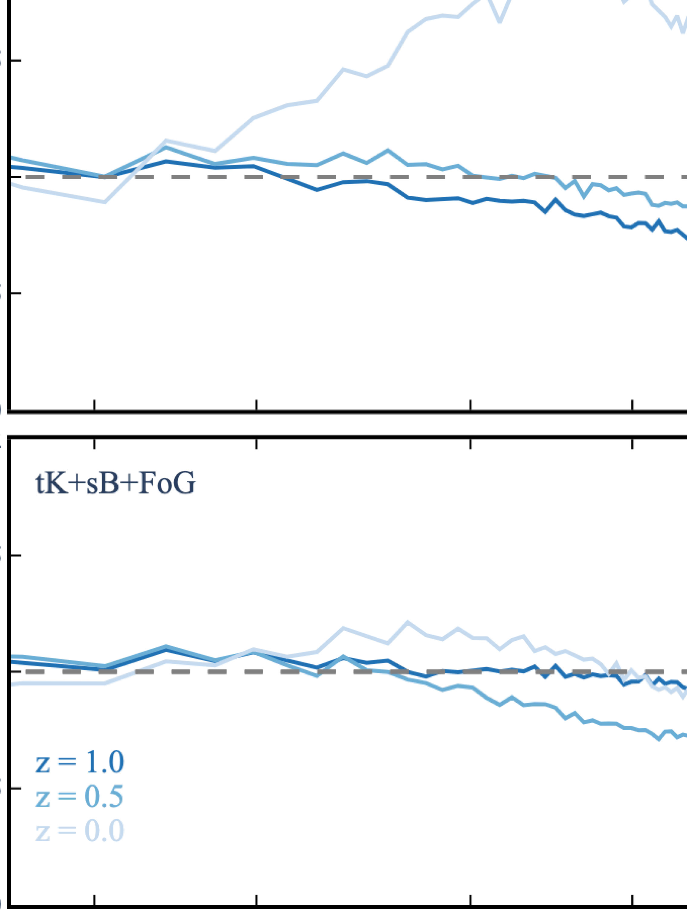
In Section 5, we examined the errors associated with various models for i auto and cross-power spectra at a single redshift. Here, we extend this analysis by characterizing some redshift trends in Fig. 14 and 15. We relegate the complete set of i-galaxy cross-power spectra and at all redshifts to the online figures as they do not yield significantly more insight into these trends.
All models in both the auto and cross power spectra perform worse at later redshifts due to stronger nonlinearities and baryonic effects. Both effects cause tracer biases to become more scale-dependent at larger scales and complicate how RSDs affect the clustering. This is particularly true at , when assuming a constant i bias introduces significant errors into the corresponding models (cB, cB+FoG, tK+cB, and tK+cB+FoG). The RSD errors in sB+FoG and tK+sB+FoG clearly manifest uniquely at as compared to the other redshifts. Attributing this phenomenon to any one process is difficult, although we note that the i-halo mass relation and i density profiles change relatively rapidly between and (see figures 4 and 5 from Villaescusa-Navarro et al., 2018).
Appendix D Comparing Auto and Cross-Power Spectra
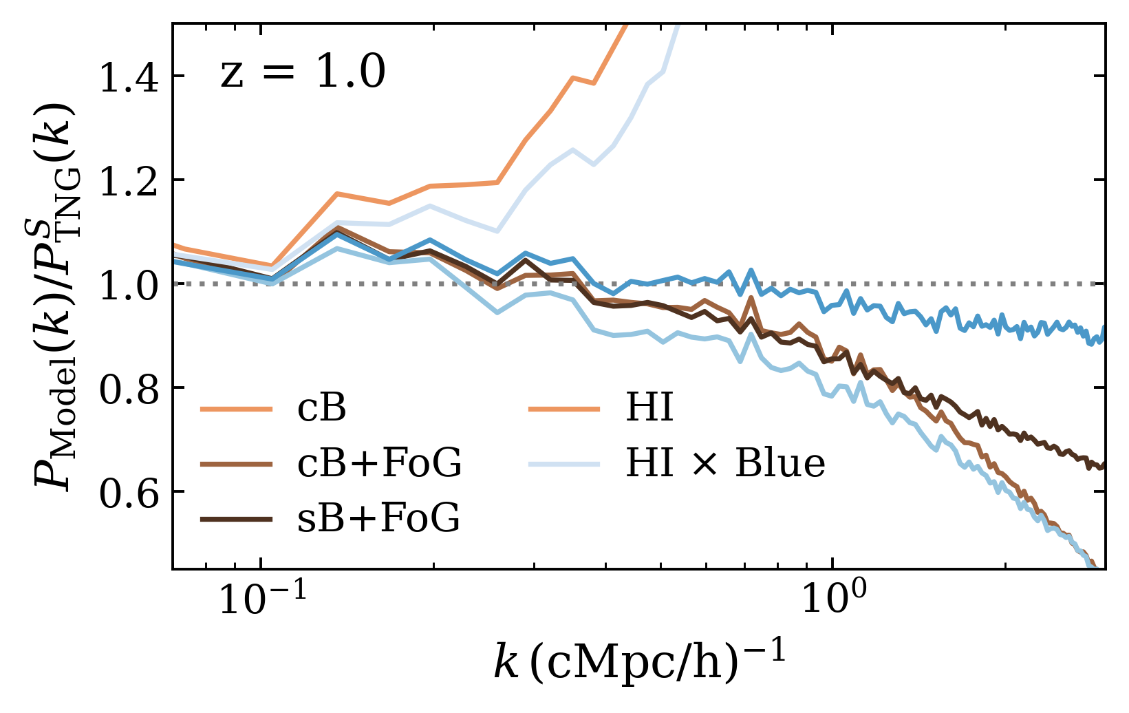
In Section 5, we studied the performance of auto and cross-power spectra separately. We can extend this analysis by comparing the best-performing cross-power spectra ( i Blue) to the i auto power spectra (Fig. 16) to gain insight into which measurement might be analytically preferred. If i Blue models outperform those of i auto power spectra, then i Blue would yield more accurate constraints on cosmological i properties, assuming any additional systematic complications arising from cross-correlating different surveys are properly handled.
Fig. 16 demonstrates that the tested models for i Blue outperform the equivalent i auto power spectrum models, or obtain comparable errors in the case of cB+FoG and tK+cB+FoG. The reason changes for each set of models. For example, tK+cB improves on cB because the FoG effect, which both models neglect, is weaker in blue galaxy clustering, reducing its overall contribution to i Blue. The weaker FoG suppression in blue galaxies also mitigates the RSD errors in tK+sB+FoG as compared to sB+FoG.
The key takeaway from Fig. 16 is that cross-correlating i and galaxy distributions can mitigate the impact of complexities in both auto power spectra, since any discrepancies between the model and the actual auto power spectra are squared but could cancel in the cross-power spectra. As an example of this, consider the i and galaxy biases. Each exhibit opposite scale-dependencies such that the product of the i and galaxy bias appears more scale-independent than either individually, mitigating errors in the cross-power spectra relative to its auto-power counterparts. Fig. 16 motivates obtaining cosmological constraints from both i auto and i-galaxy cross-power spectra as a method of testing our analytical understanding of i distributions self-consistently. However, we note that this result arises from coincidental offsets that are not present at all redshifts (online figures) and leave further analysis on the impact of the offsets on constraints from auto and cross-power spectra to future work.