What are You Looking at? Modality Contribution in Multimodal Medical Deep Learning Methods

Abstract

Purpose High dimensional, multimodal data can nowadays be analyzed by huge deep neural networks with little effort. Several fusion methods for bringing together different modalities have been developed. Particularly, in the field of medicine with its presence of high dimensional multimodal patient data, multimodal models characterize the next step. However, what is yet very underexplored is how these models process the source information in detail.

Methods To this end, we implemented an occlusion-based both model and performance agnostic modality contribution method that quantitatively measures the importance of each modality in the dataset for the model to fulfill its task. We applied our method to three different multimodal medical problems for experimental purposes.

Results Herein we found that some networks have modality preferences that tend to unimodal collapses, while some datasets are imbalanced from the ground up. Moreover, we could determine a link between our metric and the performance of single modality trained nets.

Conclusion The information gain through our metric holds remarkable potential to improve the development of multimodal models and the creation of datasets in the future. With our method we make a crucial contribution to the field of interpretability in deep learning based multimodal research and thereby notably push the integrability of multimodal AI into clinical practice. Our code is publicly available at https://github.com/ChristianGappGit/MC_MMD.

1 Introduction

Multimodal datasets, especially in the field of medicine, are becoming ever larger and more present. Thus multiple kinds of multimodal fusion methods to process this high dimensional multimodal data have been developed over the last years. It is of utmost interest to develop interpretability methods that can explain the deep learning based model’s behavior on such multimodal datasets for solving a specific task.

Possible clinical applications that use multimodal data are, for instance, the prediction of cancer prognoses [14]. Interpretability methods for the models implemented therein have the potential to generate better credibility and thus accelerate the integration of multimodal AI in general into the clinical process – "a bridge to trust between technology and human care" [3].

Interpretability methods, such as GradCAM [20] and Occlusion Sensitivity [23], have been created for single modality based networks. However, for multimodal data and models these methods are yet very underexplored. Most existing methods lack quantification of modality importance and thus inhibit comparability between models and datasets. Some existing modality importance methods either depend on the model’s performance [6, 11] or on the architecture itself [19, 10]. Others, such as attention and gradient based methods, are not sufficient to measure a modality’s importance in multimodal datasets [12].

To the best of our knowledge, we close a gap by creating a performance and model agnostic (black-box) metric to measure the modality contribution in multimodal tasks and are the first to test it on medical datasets: one image–text dataset (2D Chest X-Rays + clinical report) from Open I [1], one image–tabular dataset (2D color ophthalmological images + patient information) BRSET [18] and another image–tabular dataset (3D head and neck CT + patient information), viz. Hecktor 22 [17], published within a MICCAI grand challenge 2022.

With our metric it is possible to detect unimodal collapses, i.e. whether the model focuses extensively or even exclusively on one modality to solve a problem (e.g. [16]). Furthermore, architectures can be compared regarding their ability to process different modalities within one dataset.

First, in Section˜2 we give an overview about the state of the art in the field of interpretability in multimodal AI. Then, in Section˜3 we present our modality contribution method. Section˜4 shows details about the three medical tasks we trained in order to apply our method to in Section˜5. The results are discussed in Section˜6. We conclude with a summary and an outlook in Section˜7.

2 Related Work

The use of multimodal biomedical AI for existing large multimodal medical datasets is suggested in [2] due to its potential for clinical practice. Difficulties in understanding the models’ behavior on multimodal data make interpretability methods indispensable, as these can establish the trustworthiness of multimodal AI models [3].

In general, in order to measure a modality’s contribution to a task, performance agnostic or performance dependent metrics, model agnostic (black box model), or non-model agnostic (white box) metrics are distinguished. In [13] the authors found that attention based explainability methods can not measure single feature importance adequately. Hence methods for investigating modality contributions based on these non-model agnostic (attention) methods will suffer from the same inability to select important features. As white box’s ability to assess modality importance in multimodal tasks is controversial [12], black-box based modality importance methods are actually of utmost interest.

In [6] and [11] multimodal importance scores have been created that rely on performance metrics of the model. In contrast, [19] measures a modality’s contribution to the overall task by applying a Shapley [15] based method that is independent of performance. However, their method requires information about the architecture. Another non-model agnostic/task dependent metric is computed in [10] for efficient modality selection.

Within this work we develop a multimodal importance metric that is both model and performance agnostic.

3 Methodology – Interpretability

In the following we present our occlusion-based modality contribution method – a quantitative measure of the importance of modalities in multimodal datasets processed by multimodal neural networks.

3.1 Modality Contribution $m_{i}$

We define the metric $m_{i}\in[0,1]$ as a quantification for the contribution (importance) of the modality $i$ ($i=1,\dots,n$) in the dataset with $n$ modalities for a specific problem that was solved with a specific multimodal deep learning model. The sum over all modality contributions $\sum_{i=1}^{n}m_{i}=1$ remains constant.

Let $\vec{p}^{k}_{0}$ be the model’s output vector for the sample $k=1,\dots,N$ in the dataset with $N$ samples and $\vec{x}^{k}_{i}$ the input vector containing the features of sample $k$ for modality $i$. Then one can compute a modality specific output $\vec{p}^{k}_{i}$ for sample $k$ by manipulating $\vec{x}^{k}_{i}$ and storing the absolute difference $\vec{d}^{k}_{i}=\lvert\vec{p}^{k}_{0}-\vec{p}^{k}_{i}\rvert$. Repeating this manipulation over all samples and averaging the output differences will result in $\vec{d}_{i}=\sum_{k=1}^{N}\vec{d}_{i}^{k}/N$. After this is done for all modalities, we finally can compute

$$m_{i}=\frac{\vec{1}^{\text{\scriptsize T}}\vec{d}_{i}}{\sum_{j=1}^{n}\vec{1}^{\text{\scriptsize T}}\vec{d}_{j}}.$$ (1)

Herein the manipulation of the input vector $\vec{x}^{k}_{i}$ is the key process. It can be realized in different ways. One can mask the whole vector (i.e. the whole modality) by replacing all entries in $\vec{x}^{k}_{i}$ with zeros or with the mean of the modality specific entries in all samples, for instance. Our method works with higher resolution as we mask parts of $\vec{x}^{k}_{i}$ and repeat the forwarding process of the manipulated data to the model more often for one sample and one modality.

We split the vector $\vec{x}_{i}^{k}$ into $h_{i}$ parts and store the intermediate output distances $\vec{d}_{i,l}^{k}=\lvert\vec{p}_{0}^{k}-\vec{p}_{i,l}^{k}\rvert$, with $l=0,\dots,h_{i}-1$ before obtaining $\vec{d}_{i}^{k}=\sum_{l=0}^{h_{i}-1}\vec{d}_{i,l}^{k}$. Therein $h_{i}$ is a modality specific hyper-parameter. When processing tabular data, we can easily mask each entry in $\vec{x}^{k}_{i}$ itself ($h_{i}=\text{length}(\vec{x}_{i}^{k})$). For the vision modality we mask pixel or voxel patches in order to get interpretable results and thereby keep computation time limited due to large vision input ($h_{i}=\prod_{d=0}^{D-1}\text{img\_shape}[d]\,/\,\text{patch\_shape}[d]$, with number of image dimensions $D$).

The only criterion for $h_{i}$ is $h_{i}<h_{i,{\text{max}}}$, with upper limit $h_{i,{\text{max}}}$, where the model detects no significant differences in the output for the slightly masked input. Assuming we mask every pixel (2D) or voxel (3D), the model would not be affected sufficiently. The contribution of the vision modality would be underestimated. As long as one patch can occlude significant information, which is normally already the case for small masks too, $h_{i}$ is small enough to ensure adequate modality dependent dynamic in the model. However, choosing smaller $h_{i}$, i.e. bigger patches, is straightforward and does not affect the estimation of the model contribution substantially. Moreover it is computationally more efficient to choose big patches.

Algorithm˜1 summarizes the computation process of $m_{i}$ in the form of pseudo-code.

Algorithm 1 Computation of Modality Contribution $m_{i}$

1:$\vec{d}\leftarrow 0$

2:for $i$ in $1$ to $n$ do

3:  $\vec{d}_{i}\leftarrow 0$

4:  for $k$ in $1$ to $N$ do

5:   $\vec{x}^{k}\leftarrow$ input_k

6:   $\vec{p}_{0}^{k}\leftarrow$ model($\vec{x}^{k}$)

7:   $\vec{d}_{i}^{k}\leftarrow 0$

8:   for $l$ in $0$ to $h_{i}-1$ do

9:     $\vec{x}_{i,l}^{k}\leftarrow$ masked_input_i,l,k

10:     $\vec{p}_{i,l}^{k}\leftarrow$ model($\vec{x}_{i,l}^{k}$)

11:     $\vec{d}_{i,l}^{k}\leftarrow\lvert\vec{p}_{0}^{k}-\vec{p}_{i,l}^{k}\rvert$

12:     $\vec{d}_{i}^{k}\leftarrow\vec{d}_{i}^{k}+\vec{d}_{i,l}^{k}$

13:   end for

14:   $\vec{d}_{i}\leftarrow\vec{d}_{i}+\vec{d}_{i}^{k}/N$

15:  end for

16:  $\vec{d}\leftarrow\vec{d}+\vec{d}_{i}$

17:end for

18:for $i$ in $1$ to $n$ do

19:  $m_{i}\leftarrow\vec{1}^{\text{\scriptsize T}}\vec{d}_{i}/\vec{1}^{\text{\scriptsize T}}\vec{d}$

20:  $\vec{m}\leftarrow[\vec{m},m_{i}]$

21:end for

3.2 Modality-Specific Importance $mp_{i}^{l}$

Independent of the modality contribution to the task itself, we provide a modality specific importance distribution on patches within one modality.

The metric $mp_{i}^{l}\in[0,1]$ is defined as the contribution of a patch $l$ to the task relative to the other patches of the same modality $i$, with $l=0,\dots,h_{i}-1$. We already computed the necessary factors $\vec{d}_{i,l}^{k}$, i.e. the distance between model output $\vec{p}_{i,l}^{k}$ with masked input $\vec{x}_{i,l}^{k}$ to plain output $\vec{p}_{0}^{k}$ with unmasked input $\vec{x}^{k}$. Thus we just have to store these factors, sum over all samples to get average distance $\vec{d}_{i,l}=\sum_{k=1}^{N}\vec{d}_{i,l}^{k}/N$ and finally compute

$$mp_{i}^{l}=\frac{\vec{1}^{\text{\scriptsize T}}\vec{d}_{i,l}}{\sum_{j=0}^{h_{i}-1}\vec{1}^{\text{\scriptsize T}}\vec{d}_{i,j}}.$$ (2)

Note that $\sum_{l=0}^{h_{i}-1}mp_{i}^{l}=1$, but $\sum_{i=1}^{n}mp_{i}^{l}\not=1$, since $mp_{i}^{l}$ is modality-specific.

If we are interested in the contribution of the patch $p_{i}^{l}$ of modality $i$ to the overall task, we can simply weight $mp_{i}^{l}$ with the modality contribution $m_{i}$:

$$mp_{i}^{l}\cdot m_{i},$$ (3)

fulfilling $\sum_{i=1}^{n}\sum_{l=0}^{h_{i}-1}mp_{i}^{l}\cdot m_{i}=1$.

3.3 Metric Properties

Performance Independence

Our metric is performance agnostic as we do compute the modality contribution to a specific task by measuring the dynamic it generates in the output.

Normalization

A modality’s contribution to a specific task using a specific dataset is generated by normalizing the model’s output dynamic over all modalities using all samples in the dataset. That enables a comparison between different tasks and architectures.

Applicability

Since the computation of our metric is a black-box method, it is applicable to every multimodal dataset and every model architecture with little effort.

4 Multimodal Medical Tasks

In order to test our modality contribution method, we first trained three multimodal medical tasks, viz. two classification problems and one regression problem. For this, the architectures given in Table˜1 were built. Details on the tasks together with trainings results are presented afterwards.

Table 1: Multimodal architectures used in our experiments.

<architecture>	$\leftarrow$	<vision>	+	<text/tabular>	+	<fusion>
<ViTLLaMAII>	$\leftarrow$	<ViT>	+	<LLaMA II>	+	<Cross T.>
<ResNetLLaMAII>	$\leftarrow$	<ResNet>	+	<LLaMA II>	+	<Cross T.>
<ViTMLP>	$\leftarrow$	<ViT>	+	<MLP>	+	<MLP>
<ResNetMLP>	$\leftarrow$	<ResNet>	+	<MLP>	+	<MLP>

"ViT": Vision Transformer [4], "LLaMA II": Large Language Model Meta AI [21], "ResNet": Residual Neural Network [9], "Cross T".: Cross Transformer (with Cross Attention) [22], "MLP": Multi Layer Perceptron

4.1 Chest X-Ray + Clinical Report

4.1.1 Dataset

The image–text dataset from Open I [1] contains 2D Chest X-Rays together with a clinical report for each patient (see Fig.˜1). We used data from 3,677 patients the same way as done in [8]. In addition, we removed the class labels from the text. The 14 target classes include twelve diseases regarding the chest, especially the lungs (i.e. atelectasis, cardiomegaly, consolidation, edema, enlarged cardiomediastinum, fracture, lung lesion, lung opacity, pleural effusion, pleural other, pneumonia, pneumothorax), one for support devices and one for no finding.

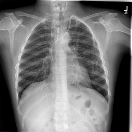
FINDINGS : The heart is normal in size. The mediastinum is within normal limits. Pectus deformity is noted. Left IJ dual-lumen catheter is visualized without pneumothorax. The lungs are clear. IMPRESSION : No acute disease.

Figure 1: Chest X-Ray + Clinical Report. Example item CXR1897_IM-0581-1001. Disease: support devices. Orange words (labels) removed during the preprocessing step.

4.1.2 Classification

For the disease classification we used the ViTLLaMAII, as already done by [5], and additionally trained a ResNetLLAMAII, a ViTMLP and a ResNetMLP. Following [5, 8], the 3,677 image–text data-pairs were split into training (3,199), validation (101) and testing (377) datasets. The classification results are presented in Table˜2.

Table 2: Performance AUC on image–text pair classification task, i.e. Chest X-Ray + clinical report, for (1) multimodal models, (2) vision (only) models and (3) clinical (only) models using the testing dataset. VL = ViTLLaMAII, RL = ResNetLLaMAII, RMLP = ResNetMLP, VMLP = ViTMLP.

	model
	(1) multimodal				(2) vision		(3) clinical
	VL	RL	RMLP	VMLP	ViT	ResNet	LLaMAII	MLP
Mean AUC	$\mathbf{0.966}$	$0.927$	$0.892$	$0.904$	$0.629$	$0.677$	$0.941$	$0.921$

4.2 BRSET

4.2.1 Dataset

The Brazilian Multilabel Ophthalmological Dataset (BRSET) [18] includes 2D color fundus retinal photos (see Fig.˜2(a)) as well as patient specific data in tabular form as presented in Table˜3. The authors provide 16,266 image–tabular data-pairs from 8,524 patients. The 14 target classes can be used for multimodal disease classification. The classes include 13 diseases (i.e. diabetic retinopathy, macular edema, scar, nevus, amd, vascular occlusion, hypertensive retinopathy, drusens, hemorrhage, retinal detachment, myoptic fundus, increased cup disc, other) and one class indicating no finding.

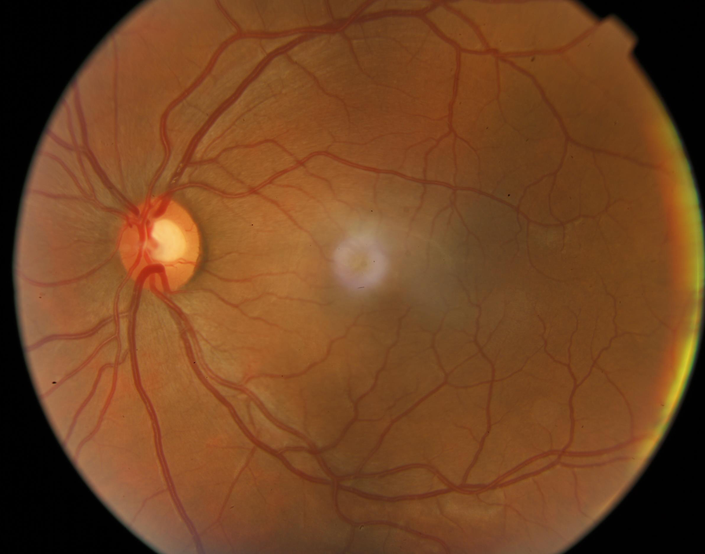
(a) source img (2390$\times$1880)

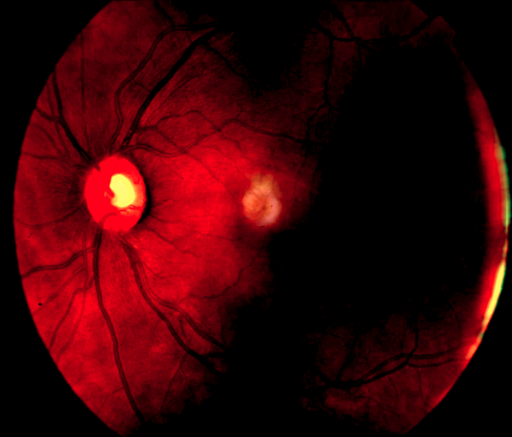
(b) transf. img (960$\times$1120)

Figure 2: BRSET. Image img01468. Preprocessing for trainings routine. The source images were normalized with mean = [0.485, 0.456, 0.406] and std = [0.229, 0.224, 0.225]. Note that black parts in the transformed image inside the eye are still distinguishable by the model.

Table 3: Tabular data in BRSET.

type	description
patient age:	age of patient in years
comorbidities:	free text of self-referred clinical antecedents
diabetes time:	self-referred time of diabetes diagnosis in years
insulin use:	self-referred use of insulin (yes or no)
patient sex:	enumerated values: 1 for male and 2 for female
exam eye:	enumerated values: 1 for the right eye and 2 for the left eye
diabetes:	diabetes diagnosis (yes or no)

4.2.2 Classification

For this multi class classification problem we trained a ResNetMLP and a ViTMLP model. We used 13,012 data-pairs for training and 3,254 for testing (i.e. a split of 80:20) in our trainings routine. Detailed performance results are presented in Table˜4.

Table 4: Performance AUC on the image–tabular pair classification task BRSET, for (1) multimodal models, (2) vision (only) models and (3) clinical (only) models using the testing dataset.

	model
	(1) multimodal		(2) vision		(3) clinical
	ResNetMLP	ViTMLP	ResNet	ViT	MLP
Mean AUC	$\mathbf{0.907}$	$0.798$	$0.899$	$0.724$	$0.669$

4.3 Hecktor 22

4.3.1 Dataset

The head and neck tumor segmentation training dataset contains data from 524 patients. For each patient 3D CT, 3D PET images and segmentation masks of the extracted tumors are provided together with clinical information in the form of tabular data as presented in Table˜5. For the RFS (Relapse Free Survival) time prediction task, i.e. a regression problem, labels (0,1), indicating the occurrence of relapse and the RFS times (for label 0) and the PFS (Progressive Free Survival) times (label 1) in days are made available for 488 patients. Due to some incomplete data and non-fitting segmentation masks, we finally could use image–tabular data pairs (CT segmentation mask + tabular data) of 444 patients.

Table 5: Tabular data in Hecktor 22.

type	description
gender:	male (M), female (F)
age:	patient age in years
weight:	patient weight in kg
tobacco:	smoker (1), non-smoker (0)
alcohol:	drinks regularly (1), non-alcoholic (0)
performance status:	1 or 0
HPV status:	positive (1), negative (0)
surgery:	had a surgery (1), no surgery (0)
chemotherapy:	gets chemotherapy (1), no chemotherapy (0)

4.3.2 Regression

For the regression we used the ResNetMLP and the ViTMLP models, with Rectified Linear Units (ReLUs) as activation functions here. For the RFS, PFS regression training we used data from 355 patients for training and 89 patients for testing, i.e. a split of approximately 80:20. Table˜6 provides detailed results.

Table 6: Performance c-index on image–tabular regression task, viz. Hecktor 22, for (1) multimodal models, (2) vision (only) models and (3) clinical (only) models on the testing dataset. Here the results are for the RFS prediction, i.e. the observed class is label 1: relapse.

	model
	(1) multimodal		(2) vision		(3) clinical
	ResNetMLP	ViTMLP	ResNet	ViT	MLP
c-index	$0.705$	$0.605$	$\mathbf{0.709}$	$0.678$	$0.572$

5 Experiments and Results

For both classification tasks and the regression problem we present our quantitative metric $m_{i}$ to measure the modality contributions. In Table˜7 the results are summarized. For datasets BRSET and Hecktor 22 we also present the modality specific importance $mp_{i}^{l}$.

Table 7: Modality contribution specific for architecture and dataset. Entries quantify $m_{0}$ to $m_{1}$, viz. vision : text (Chest X-Ray) and vision : tabular (BRSET, Hecktor 22). The computation was done on the testing datasets.

Model	Chest X-Ray	BRSET	Hecktor 22
ResNetLLaMAII	$0.18:0.82$
ViTLLaMAII	$0.13:0.87$
ResNetMLP	$0.59:0.41$	$0.92:0.08$	$0.65:0.35$
ViTMLP	$0.02:0.98$	$0.67:0.33$	$0.00:1.00$

5.1 Multiclass Classification with Chest X-Ray + Clinical Report

In Table˜7, second column, the $m_{i}$ results are printed for four different multimodal nets. The computations were done with $h_{i}=\{$vision: 196, text: number of words in report$\}$. The visualization results and analyses are presented in Fig.˜3.

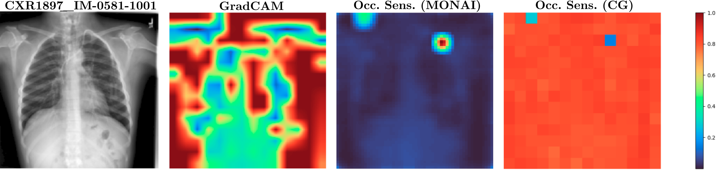
Figure 3: CXR1897_IM-0581-1001: Correctly predicted disease: support devices. Modality contribution vision : text = 0.24 : 0.76. Model: ViTLLAMA II. From blue to red the contribution (low to high) from a single patch (vision) or word (text) to the task is highlighted. Top, left to right: source image, GradCAM, class specific Occlusion Sensitivity for class support devices (MONAI), Occlusion Sensitivity averaged over all classes (CG, i.e. ours). The red patch in the upper right area in image Occ. sens. (MONAI) has the highest contribution to the class support devices. The same area is colored blue in image Occ. sens. (CG), as this patch has the lowest average contribution to all classes. Bottom: Text. MEAN: The words no and acute have the highest average contribution, catheter has the lowest. MAX: catheter has the highest contribution to one class: support devices.

5.2 Multiclass Classification with BRSET

The third column of Table˜7 shows the $m_{i}$ results for the two trained nets. Modality Contribution ratios (vision : tabular) are $0.92:0.08$ for ResNetMLP and $0.67:0.33$ for ViTMLP. The computations were done with $h_{i}=\{$vision: 240, tabular: 7$\}$. The visualization results are presented in Fig.˜4 together with explanations. The token importance for tabular data is presented in Table˜8.

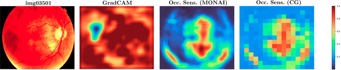
Figure 4: img03501: Correctly predicted disease: drusens. Modality contribution vision : tabular = 0.95 : 0.05. Model: ResNetMLP. Importance (low to high) is colored from blue to red. Top, left to right: source image, GradCAM, class specific Occlusion Sensitivity for class drusens (MONAI), Occlusion Sensitivity averaged over all classes (CG, i.e. ours). Bottom: tabular data with attributes patient age, comorbidities, diabetes time, insulin use, patient sex, exam eye, diabetes from left to right. MEAN: The patient’s age has the highest contribution, patient sex the lowest in average. MAX: patient’s age is the most significant attribute for one class: drusens.

Table 8: Modality Contribution $m_{i}^{l}$ and $mp_{i}^{l}$ with $l=0,\dots,h_{i}-1$ and $h_{i}=7$ for the tabular data in the BRSET classification problem. The three most important attributes per $mp_{i}^{l}$-column are highlighted in bold.

	ResNetMLP		ViTMLP
	$m_{i}^{l}$	$mp_{i}^{l}$	$m_{i}^{l}$	$mp_{i}^{l}$	$l$
patient age:	$0.024$	$\mathbf{0.289}$	$0.081$	$\mathbf{0.245}$	$0$
comorbidities:	$0.008$	$0.093$	$0.025$	$0.076$	$1$
diabetes time:	$0.011$	$\mathbf{0.133}$	$0.063$	$\mathbf{0.192}$	$2$
insulin use:	$0.009$	$0.110$	$0.047$	$0.143$	$3$
patient sex:	$0.010$	$0.124$	$0.018$	$0.056$	$4$
exam eye:	$0.006$	$0.091$	$0.033$	$0.100$	$5$
diabetes:	$0.013$	$\mathbf{0.160}$	$0.062$	$\mathbf{0.188}$	$6$
sum:	$0.081$	$1.000$	$0.329$	$1.000$

5.3 Regression – RFS Prediction with Hecktor 22

For the computation of the modality contribution for the RFS prediction task we have chosen $h_{i}=\{$vision: 8, tabular: 9$\}$. The big mask, i.e. half of image size in each dimension ($2^{-3}=8^{-1}$) for vision is necessary to occlude enough from the segmented tumor. With ResNetMLP we have computed a modality contribution vision : tabular = 0.65 : 0.35 (see Table˜7: fourth column). For ViTMLP we have vision : tabular = 0.0 : 1.0 (unimodal collapse). Table˜9 shows the results for the token importance for the tabular data.

Table 9: Modality Contribution $m_{i}^{l}$ and $mp_{i}^{l}$ with $l=0,\dots,h_{i}-1$ and $h_{i}=9$ for tabular data in Hecktor 22 regression problem. Architecture: ResNetMLP. The three most important attributes are highlighted in bold.

	$m_{i}^{l}$	$mp_{i}^{l}$	$l$
gender	0.054	0.156	0
age	0.069	0.197	1
weight	0.068	0.196	2
tobacco	0.002	0.007	3
alcohol	0.034	0.097	4
performance status	0.003	0.008	5
HPV status	0.088	0.254	6
surgery	0.006	0.018	7
chemotherapy	0.023	0.067	8
sum	0.347	1.000

6 Discussion

For the classification task with the image–text dataset from [1], viz. Chest X-Ray + clinical report, we computed the modality contribution $m_{i}$ between vision and text. Our results for this dataset confirm the behavior found in [7], that the text modality is the most important modality in most multimodal datasets containing text.

Results also show that our multimodal models that contain a Residual Neural Network (ResNet) [9] instead of a Vision Transformer (ViT) [4] have a bigger ratio between the vision and text modality contribution for our tasks.

Unimodal collapses occured in two cases: (1) ViTMLP for Chest X-Ray + clinical report and (2) ViTMLP for Hecktor 22. ResNetMLP for BRSET has a tendency to collapse with 92% vision to only 8% tabular contribution. While in (1) the ViTMLP does almost not use the vision modality, it is completely ignored in (2). The ViTMLP only works well for the classification task with BRSET.

Another outcome is that we can determine a link between our metric and the performance of single modality trained nets. The higher the contribution of a modality $i$ to a task, the higher the performance of a net that was only trained with modality $i$ (compare $m_{0}$ and $m_{1}$ from Table˜7 with vision and clinical net’s mean performances from Table˜2, Table˜4, Table˜6).

7 Summary and Outlook

Due to high dimensional multimodal data availability in several fields, especially in medicine, deep learning based multimodal fusion methods were developed. In order to better understand deep learning based models, interpretability methods are widely used. This ensures the trustworthiness of the models, which is a basic requirement in the medical field.

Therefore, we created a powerful metric to analyze deep learning models regarding modality preference in multimodal datasets and to highlight important attributes within one modality. In contrast to existing methods [6, 11, 19, 10], our method is both fully model and performance agnostic.

We trained three different multimodal datasets, one image–text for classification and two image–tabular for classification and regression respectively, and evaluated the models on the testing datasets. Then we applied our new method on them. We could show that some architectures process multimodal data in a balanced way, while others tend to unimodal collapses. Furthermore, import attributes within one modality were quantitatively highlighted.

Our occlusion based modality contribution has a user specific hyper-parameter for continuous data, i.e. $h_{i}$. In contrast to text or tabular data these lack natural sequencing. Although the vision modality is discrete, it also lacks natural sequencing due to dependencies of resolution and displayed content. As a consequence, the length of the occluded sequences $h_{i}$ for continuous data, and for modalities such as vision, must be chosen small enough (i.e. big enough patches) to occlude sensitive information. We recommend focusing further research on how the choice of $h_{i}$ for this type of data affects the modality contribution metric $m_{i}$.

With the information of modality contribution in multimodal (medical) datasets, deep learning based multimodal networks can be chosen properly or, in case of unimodal collapse for instance, redesigned to use all modalities and thereby exploit the full potential of the multimodal datasets. We are convinced that our method will significantly advance the integrability of multimodal AI in general into clinical practice. Our code is publicly available at https://github.com/ChristianGappGit/MC_MMD.

7.0.1 Acknowledgements

This study is partly supported by VASCage – Centre on Clinical Stroke Research.

7.0.2

The authors have no competing interests to declare that are relevant to the content of this article.

References

- [1] Open-I: An open access biomedical search engine. https://openi.nlm.nih.gov, accessed: 2023-12-20
- [2] Acosta, J.N., Falcone, G.J., Rajpurkar, P., Topol, E.J.: Multimodal biomedical AI. Nature Medicine 28(9), 1773–1784 (09 2022). https://doi.org/10.1038/s41591-022-01981-2
- [3] Beger, J.: The crucial role of explainability in healthcare AI. European Journal of Radiology 176 (07 2024). https://doi.org/10.1016/j.ejrad.2024.111507
- [4] Dosovitskiy, A., Beyer, L., Kolesnikov, A., Weissenborn, D., Zhai, X., Unterthiner, T., Dehghani, M., Minderer, M., Heigold, G., Gelly, S., Uszkoreit, J., Houlsby, N.: An image is worth 16x16 words: Transformers for image recognition at scale. In: International Conference on Learning Representations (2021)
- [5] Gapp, C., Tappeiner, E., Welk, M., Schubert, R.: Multimodal medical disease classification with LLaMA II (2024), https://arxiv.org/abs/2412.01306, The First Austrian Symposium on AI, Robotics, and Vision (AIROV24) – (in press)
- [6] Gat, I., Schwartz, I., Schwing, A.: Perceptual score: What data modalities does your model perceive? In: Ranzato, M., Beygelzimer, A., Dauphin, Y., Liang, P., Vaughan, J.W. (eds.) Advances in Neural Information Processing Systems. vol. 34, pp. 21630–21643. Curran Associates, Inc. (2021)
- [7] Haouhat, A., Bellaouar, S., Nehar, A., Cherroun, H.: Modality influence in multimodal machine learning (2023), https://arxiv.org/abs/2306.06476
- [8] Hatamizadeh, A.: TransCheX: Self-supervised pretraining of vision-language transformers for chest X-ray analysis (2021), https://github.com/Project-MONAI/tutorials/blob/main/multimodal (Accessed: 2023-19-03)
- [9] He, K., Zhang, X., Ren, S., Sun, J.: Deep residual learning for image recognition. In: 2016 IEEE Conference on Computer Vision and Pattern Recognition (CVPR). pp. 770–778 (06 2016). https://doi.org/10.1109/CVPR.2016.90
- [10] He, Y., Cheng, R., Balasubramaniam, G., Tsai, Y.H.H., Zhao, H.: Efficient modality selection in multimodal learning. Journal of Machine Learning Research 25(47), 1–39 (2024), http://jmlr.org/papers/v25/23-0439.html
- [11] Hu, P., Li, X., Zhou, Y.: SHAPE: An unified approach to evaluate the contribution and cooperation of individual modalities. In: Raedt, L.D. (ed.) Proceedings of the Thirty-First International Joint Conference on Artificial Intelligence, IJCAI-22. pp. 3064–3070. International Joint Conferences on Artificial Intelligence Organization (7 2022). https://doi.org/10.24963/ijcai.2022/425, main Track
- [12] Jain, S., Wallace, B.C.: Attention is not Explanation. In: Burstein, J., Doran, C., Solorio, T. (eds.) Proceedings of the 2019 Conference of the North American Chapter of the Association for Computational Linguistics: Human Language Technologies, Volume 1 (Long and Short Papers). pp. 3543–3556. Association for Computational Linguistics, Minneapolis, Minnesota (Jun 2019). https://doi.org/10.18653/v1/N19-1357
- [13] Jin, W., Li, X., Hamarneh, G.: Evaluating explainable AI on a multi-modal medical imaging task: Can existing algorithms fulfill clinical requirements? Proceedings of the AAAI Conference on Artificial Intelligence 36(11), 11945–11953 (Jun 2022). https://doi.org/10,1609/aaai.v36i11.21452
- [14] Lobato-Delgado, B., Priego-Torres, B., Sanchez-Morillo, D.: Combining molecular, imaging, and clinical data analysis for predicting cancer prognosis. Cancers 14(13) (2022). https://doi.org/10.3390/cancers14133215, https://www.mdpi.com/2072-6694/14/13/3215
- [15] Lundberg, S.M., Lee, S.I.: A unified approach to interpreting model predictions. In: Guyon, I., Luxburg, U.V., Bengio, S., Wallach, H., Fergus, R., Vishwanathan, S., Garnett, R. (eds.) Advances in Neural Information Processing Systems. vol. 30. Curran Associates, Inc. (2017)
- [16] Madhyastha, P.S., Wang, J., Specia, L.: Defoiling foiled image captions. In: Walker, M., Ji, H., Stent, A. (eds.) Proceedings of the 2018 Conference of the North American Chapter of the Association for Computational Linguistics: Human Language Technologies, Volume 2 (Short Papers). pp. 433–438. Association for Computational Linguistics, New Orleans, Louisiana (Jun 2018). https://doi.org/10.18653/v1/N18-2069
- [17] MICCAI: HEad and neCK TumOR segmentation and outcome prediction in PET/CT images (third edition) (8 2022), https://hecktor.grand-challenge.org/Data/
- [18] Nakayama, L.F., Restrepo, D., Matos, J., Ribeiro, L.Z., Malerbi, F.K., Celi, L.A., Regatieri, C.S.: BRSET: A brazilian multilabel ophthalmological dataset of retina fundus photos. PLOS Digital Health 3(7), 1–16 (07 2024). https://doi.org/10.1371/journal.pdig.0000454
- [19] Parcalabescu, L., Frank, A.: MM-SHAP: A performance-agnostic metric for measuring multimodal contributions in vision and language models & tasks. In: Proceedings of the 61st Annual Meeting of the Association for Computational Linguistics (Volume 1: Long Papers). Association for Computational Linguistics (2023). https://doi.org/10.18653/v1/2023.acl-long.223
- [20] Selvaraju, R.R., Cogswell, M., Das, A., Vedantam, R., Parikh, D., Batra, D.: Grad-CAM: Visual explanations from deep networks via gradient-based localization. In: 2017 IEEE International Conference on Computer Vision (ICCV). pp. 618–626 (2017). https://doi.org/10.1109/ICCV.2017.74
- [21] Touvron, H., Martin, L., Edunov, S., Scialom, T.: Llama 2: Open foundation and fine-tuned chat models (2023), https://arxiv.org/abs/2307.09288
- [22] Xu, P., Zhu, X., Clifton, D.A.: Multimodal learning with transformers: A survey. IEEE Transactions on Pattern Analysis & Machine Intelligence 45(10), 12113–12132 (10 2023). https://doi.org/10.1109/TPAMI.2023.3275156
- [23] Zeiler, M.D., Fergus, R.: Visualizing and understanding convolutional networks. In: Fleet, D., Pajdla, T., Schiele, B., Tuytelaars, T. (eds.) Computer Vision – ECCV 2014. pp. 818–833. Springer International Publishing, Cham (2014)