Hilbert’s Sixth Problem: derivation of fluid equations via Boltzmann’s kinetic theory
Abstract.
In this paper, we rigorously derive the fundamental PDEs of fluid mechanics, such as the compressible Euler and incompressible Navier-Stokes-Fourier equations, starting from the hard sphere particle systems undergoing elastic collisions. This resolves Hilbert’s sixth problem, as it pertains to the program of deriving the fluid equations from Newton’s laws by way of Boltzmann’s kinetic theory. The proof relies on the derivation of Boltzmann’s equation on 2D and 3D tori, which is an extension of our previous work [26].
1. Introduction
1.1. Hilbert’s sixth problem
In his address to the International Congress of Mathematics in 1900, David Hilbert proposed a list of problems as challenges for the mathematics of the new century. Of those problems, the sixth problem asked for an axiomatic derivation of the laws of physics. In his description of the problem, Hilbert says:
"The investigations on the foundations of geometry suggest the problem: To treat in the same manner, by means of axioms, those physical sciences in which already today mathematics plays an important part; in the first rank are the theory of probabilities and mechanics."
Broadly interpreted, this problem can encompass all of modern mathematical physics. However, in his followup article [35], which describes and elaborates on the list of problems, Hilbert specified two concrete questions under this sixth problem. The first concerns the axiomatic foundation of probability, which was settled in the first half of the twentieth century. The second question was described as follows:
"...Boltzmann’s work on the principles of mechanics suggests the problem of developing mathematically the limiting processes, there merely indicated, which lead from the atomistic view to the laws of motion of continua."
In this question, Hilbert suggests a program, referred to as Hilbert’s program below, which aims at giving a rigorous derivation of the laws of fluid motion, starting from Newton’s laws on the atomistic level, using Boltzmann’s kinetic theory as an intermediate step. More precisely, this refers to giving a rigorous justification of the following diagram:
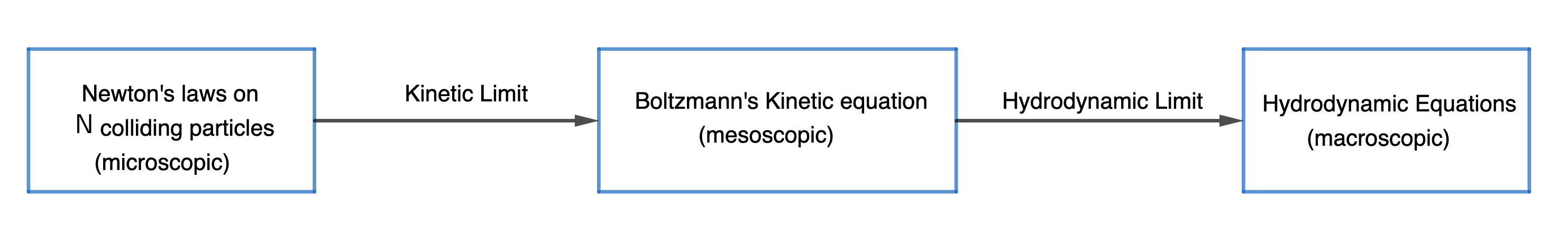
In this paper we will complete Hilbert’s program and justify the limiting process in Figure 1. We start by describing the scope of this program and its two steps, as well as the historical accounts.
In the first step of this program, one gives a rigorous derivation of Boltzmann’s kinetic theory starting from Newton’s laws, taken as axioms, on a microscopic system formed of particles of diameter undergoing elastic collisions. This is done by taking the kinetic limit in which , and we aim to show that the one-particle density of the particle system is well-approximated by the solution to the Boltzmann equation:
| (1.1) |
Here is the hard-sphere collision kernel defined below in (1.15), and stands for the collision rate of the particle system, which is kept constant in this kinetic limit. The necessity of this scaling relation between and , which corresponds to the setting of dilute gases, was discovered by Grad [31], and is referred to as the Boltzmann-Grad limit. In the second step, called the hydrodynamic limit, one derives the equations of fluid mechanics (like compressible Euler, incompressible Euler, incompressible Navier-Stokes etc.) as appropriate limits of Boltzmann’s kinetic equation when the collision rate is taken to infinity (i.e. the Knudson number, or the length of mean free path, is taken to zero).
To complete Hilbert’s original program, one needs to take a proper combination of these two limits, to pass from the atomistic view of matter to the laws of motion of continua, as Hilbert put it in his own words. Crucially, here we note that establishing the link between these two limits requires deriving the Boltzmann equation as stated above on time intervals of length , which corresponds (by rescaling and ) to solutions of the Boltzmann equation that exist on time intervals of length . Since in the hydrodynamic limit, it is thus necessary to obtain long time derivation of the Boltzmann equation.
In the two limits, the first (kinetic) limit turned out to be more challenging. In fact, it even took some time to properly clarify it as a concrete mathematical question. This was eventually done by Grad [31] who specified the precise Boltzmann-Grad scaling law mentioned above, which is assumed between the number of particles and their diameter , in order for Boltzmann’s kinetic theory to be valid in the limit . Following several pioneering works of Grad [31] and Cercignani [18], the first major landmark in the derivation of Boltzmann’s equation happened in 1975, when Lanford [42] first completed this derivation for sufficiently small times. After Lanford’s work, the problem of deriving Boltzmann’s equation has attracted a tremendous amount of research interest from various angles and perspectives [41, 40, 45, 46, 47, 38, 49, 54, 56, 52]. We single out particularly the progress in the past fifteen years which reinvigorated the effort of fully executing Hilbert’s program, thanks to the deep works of various subsets of the following authors: Bodineau, Gallagher, Pulvirenti, Saint Raymond, Simonella, Texier [28, 50, 51, 5, 6, 7, 8, 9, 10, 11, 13, 12]. We note that all those results are restricted to either short times, or small (near-vaccuum) solutions, or various linearized settings. Such restrictions represented, for the longest time, the major obstruction to fully executing Hilbert’s program, which requires accessing long-time solutions of the Boltzmann equation, as described in the above paragraph.
This barrier was finally broken in the authors’ recent work [26] which gave the rigorous derivation of Boltzmann’s equation on for arbitrarily long times, namely as long as the strong solution to Boltzmann’s equation exists.
Compared to the first kinetic limit, the second hydrodynamic limit was better understood earlier on. The rough idea here, which was explained by Hilbert himself in [36], is that the local Maxwellians
are approximate solutions to the Boltzmann equation, in the limit , provided that the macroscopic quantities solve a corresponding hydrodynamic equation. The results in this direction can be split according to whether they address strong or weak solutions. In the case of strong solutions, we mention the works of Nishida [48] and Caflisch [17] for the incompressible and compressible Euler limit and the works of DeMasi-Esposito-Liebowitz [20], Bardos-Ukai [4], Guo [32] for the incompressible Euler and Navier-Stokes limits. Below we also rely on the more recent works of Gallagher and Tristani [29] for the incompressible Navier-Stokes limit, and of Guo-Jang-Jiang [34] and Jiang-Luo-Tang [39] for the compressible Euler limit. In the case of weak solutions, we mention the works of Bardos-Golse-Levermore [2, 3], Lions-Masmoudi [43, 44], Golse-Saint Raymond [30], and refer the reader to the textbook treatment in [53].
The purpose of this work is twofold. First we extend the derivation of Boltzmann’s equation in [26] to the periodic setting . Second, we connect this kinetic limit to the hydrodynamic limit in the above-cited works, to obtain a full derivation of the fluid equations starting from Newton’s laws on the particle system, thereby completing Hilbert’s original program. We summarize the main theorems as follows:
-
•
Theorem 1: Derivation of the Boltzmann equation on . Starting from a Newtonian hard-sphere particle system on the torus formed of particles of diameter undergoing elastic collisions, and in the Boltzmann-Grad limit , we derive the Boltzmann equation (1.1) as the effective equation for the one-particle density function of the particle system.
-
•
Theorem 2: Derivation of the incompressible Navier-Stokes-Fourier system from Newton’s laws. Starting from the same Newtonian hard-sphere particle system on the torus close to global equilibrium, and in an iterated limit where first with fixed and then separately (there are also other variants, see Theorem 2), we derive the incompressible Navier-Stokes-Fourier system as the effective equation for the macroscopic density and velocity of the particle system.
-
•
Theorem 3: Derivation of the compressible Euler equation from Newton’s laws. Starting from the same Newtonian hard-sphere particle system on the torus , and in an iterated limit where first with fixed and then separately (there are also other variants, see Theorem 3), we derive the compressible Euler equation as the effective equation for the macroscopic density, velocity, and temperature of the particle system.
A fundamental intriguing question is the justification of the passage from the time-reversible microscopic Newton’s theory to the time-irreversible mesoscopic Boltzmann theory. It is well-known (see [55] for smooth data and [33] for data, also [27] for large-amplitude renormalized solutions) that solutions to Boltzmann’s equation are global-in-time near any Maxwellian, and the celebrated Boltzmann H-theorem indicates the increase of physical entropy and time irreversibility in the Boltzmann theory. Since Theorem 1 covers the full lifespan of the Boltzmann solution, it could be viewed as a justification of the emergence of the time irrevsesible Boltzmann theory from the time reversible Newton’s theory near Maxwellian.
We shall give the precise statement of Theorems 1–3 in the next sections, together with the proofs of Theorems 2 and 3 which will follow directly by combining Theorem 1 with the existing results on the hydrodynamic limit. The proof of Theorem 1 follows the same lines as the Euclidean setting in [26], except for one particular part of the proof which requires substantial modifications. For this, a different algorithm is introduced to deal with a particular set of collision histories that can arise in the periodic setting. The key difference, which necessitates both new algorithms and new integral estimates in the latter setting, is the absence of upper bound on the number of collisions that can happen among a fixed number of particles (in contrast with the Euclidean case where the particles eventually move away from each other).
1.2. From Newton to Boltzmann
We start by describing the microscopic hard-sphere particle dynamics, and the Boltzmann equation which describes the limits of the -particle density functions determined by such dynamics.
1.2.1. The hard sphere dynamics
Throughout this paper, we fix the periodic torus in dimension . For , define to be the distance between and the origin ; if we view as a vector in (understood modulo ), then
| (1.2) |
If satisfies , then is represented by a unique vector satisfying in the Euclidean norm of . Below we will always identify this with (and do not distinguish it with in writing) without further explanations.
Definition 1.1 (The hard-sphere dynamics [1]).
We define the hard sphere system of particles with diameter , in dimension .
-
(1)
State vectors and . We define and , where and are the center of mass and velocity of particle ; this and are called the state vector of the -th particle and the collection of all particles, respectively.
-
(2)
The domain . We define the non-overlapping domain as
(1.3) -
(3)
The hard-sphere dynamics . Given initial configuration , we define the hard sphere dynamics as the time evolution of the following dynamical system:
-
(a)
We have .
-
(b)
Suppose is known for . If for some , then we have
(1.4) Here indicates right limit at time , see Figure 2. Note that are always continuous in ; in this definition we also always require to be left continuous in , so .
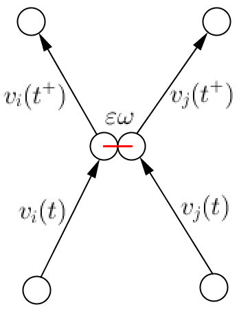
Figure 2. An illustration of the hard sphere dynamics (Definition 1.1 (3b)): and are incoming and outgoing velocities, and is the vector connecting the centers of the two colliding particles, which has length . - (c)
-
(a)
-
(4)
The flow map and flow operator . We define the flow map by
(1.6) where is defined by (3). Define also the flow operator , for functions , by
(1.7) - (5)
1.2.2. The grand canonical ensemble
Define the grand canonical domain , so always represents for some . We can define the hard sphere dynamics and the flow map on , by specifying them to be the and in Definition 1.1 (3)–(4), for initial configuration .
The grand canonical ensemble is defined by a density function (or equivalently a sequence of density functions ), which determines the law of the random initial configuration for the hard-sphere system, as follows.
Definition 1.3 (The grand canonical ensemble).
Fix and , and a nonnegative function with . We define the grand canonical ensemble as follows.
-
(1)
Random configuration and initial density. Assume is a random variable, whose law is given by the initial density function , in the sense that
(1.8) for any and any , where is given by
(1.9) Here, is the indicator function of the set , and the partition function is defined to be
(1.10) -
(2)
Evolution of random configuration. Let be the random variable defined in (1) above, and let be the evolution of initial configuration by hard sphere dynamics, defined in Definition 1.1 (3)–(4), then is also a -valued random variable. We define the density functions for the law of the random variable by the relation
(1.11) Then it is easy to see (using the volume preserving property in Proposition 1.2) that
(1.12) -
(3)
The correlation function . Given , we define the -particle (rescaled) correlation function by the following formula
(1.13) where we abbreviate and similar to .
-
(4)
The Boltzmann-Grad scaling law. The definition (1.9), and particularly the choice of the factor , implies that
(1.14) up to error , where is the random initial data defined in (1) and is the random variable (i.e. number of particles) determined by . If is a constant, then we are considering the hard sphere dynamics with particles (on average). This is referred to as the Boltzmann-Grad scaling law.
1.2.3. The Boltzmann equation
The kinetic theory predicts that the one-particle correlation function should solve the Boltzmann equation in the kinetic limit , which is defined as follows.
Definition 1.4 (The hard-sphere Boltzmann equation).
We define the Cauchy problem for the Boltzmann equation for hard sphere collisions, with initial data where , as follows:
| (1.15) |
The right hand side of (1.15) is referred to as the collision operator, where is the positive part of , and we denote
1.2.4. Main result 1
We now state the first main result of this paper.
Theorem 1.
Fix and . Let be three parameters that satisfy
| (1.16) |
where the implicit constant in (1.16) depends only on . Let be a nonnegative function with , and suppose the solution to the Boltzmann equation (1.15) exists on the time interval , such that
| (1.17) |
Consider the dimensional hard sphere system of diameter particles (Definition 1.1), with random initial configuration given by the grand canonical ensemble (Definition 1.3), under the Boltzmann-Grad scaling law (1.14). Let be small enough depending on and the implicit constant in (1.16). Then, uniformly in and in , the -particle correlation functions defined in (1.9)–(1.13), satisfy that
| (1.18) |
where is an absolute constant depending only on the dimension .
Remark 1.5.
We make a few remarks concerning Theorem 1.
(1) For simplicity of the proof, we have restricted to dimension in Theorems 1–3. For we believe the result should still be true, but both the algorithm and the integral parts of the proof will get considerably more sophisticated for larger , see Remark 1.9.
(2) In (1.16) we have assumed . Improving this bound amounts to allowing for a wider range of in the limit in Theorems 2–3. However, such an improvement seems to be hard with our methods, see Part 7 of Section 5.
(3) Note that (1.17) requires one more derivative on than the bound we can prove in (1.18). This loss of derivatives can easily be reduced to for any small constant or , by exactly the same proof; it can also be eliminated (i.e. ), but one will need to assume the to be independent of instead of allowing the growth in (1.16).
1.3. From Newton to Euler and Navier-Stokes
It is well known [17, 20, 29, 30] that in suitable limits where , solutions to the Boltzmann equation (1.15) that have local Maxwellian form (i.e. being Gaussian in ) can be described by solutions to the corresponding fluid equations, which is referred to as the hydrodynamic limit in the literature.
Now, by combining Theorem 1 with such results, we can obtain these fluid limits from the colliding particle systems in Definitions 1.1 and 1.3, via the Boltzmann equation (1.15). We consider only two examples in this subsection, which correspond to the incompressible Navier-Stokes-Fourier and the compressible Euler equations.
1.3.1. Main result 2: the incompressible Navier-Stokes-Fourier limit
We first recall the following hydrodynamic limit result in Gallagher-Tristani [29]; see also Bardos-Ukai [4].
Proposition 1.6 ([29]).
Let , consider the coupled incompressible Navier-Stokes-Fourier equations on :
| (1.19) |
where and are two positive absolute constants depending on ; for exact expressions see [29]. Here the in (1.19) is valued in , and have zero mean in (which is preserved by (1.19)). We fix a smooth solution to (1.19) on an arbitrary time interval with initial data , and also fix an initial perturbation such that it has zero mean in for each , and
| (1.20) |
Now, for sufficiently small , consider the Boltzmann equation (1.15) with , and (well prepared) initial data given by
| (1.21) |
Note that we may choose to make nonnegative, and it also satisfies by (1.21). Then, for , we have
| (1.22) |
where the remainder satisfies the following estimate uniformly in :
| (1.23) |
Proof.
This is the same as the proof of Theorem 1.1 in [29]. We only make a few remarks here:
(1) In [29] the Navier-Stokes-Fourier system (1.19) is stated in terms of three unknown functions , but also with the restriction , which makes it equivalent to the current formulation (1.19).
(2) The initial data (1.21) corresponds to the well-prepared case in the notion of [29], plus a small remainder term . It is clear, by examining the proof in [29], that this perturbation does not affect any of the linear and bilinear estimates there, thus the same proof in [29] carries out and leads to the same result (1.22).
Now we can state our second main result, concerning the passage from colliding particle systems to the incompressible Navier-Stokes-Fourier equation:
Theorem 2.
Let , consider two small parameters . Also fix a smooth solution to the Navier-Stokes-Fourier equation (1.19) on an arbitrary time interval . Here we understand that, if the solution is global in time, then is allowed to grow to infinity as ; otherwise it is independent of , and in any case we assume the following relation between the parameters
| (1.24) |
with the same implicit constant as in (1.16). We also fix as in (1.20).
Now, consider the hard sphere system of diameter particles (Definition 1.1), with random initial configuration given by the grand canonical ensemble (Definition 1.3), where and defined as in (1.21). Note that this corresponds to the (expected) number of particles
| (1.25) |
which is the Boltzmann-Grad scaling (1.14) when is constant, or barely more dense than that when is a negative power of (see (1.24)). Let be the -particle correlation function defined in (1.9)–(1.13) with . Then we have the followings:
- (1)
-
(2)
Let be any test function in . For each fixed , consider the random variables
(1.28) associated with the hard sphere system under the random initial configuration assumption. Then, in the limit as described in (1) above, we have the convergence
(1.29) in probability.
Remark 1.7.
The equalities (1.27) and (1.29) show that the fluid parameters and can be obtained by directly taking limits of the associated statistical quantities coming from the hard sphere dynamics. The velocity truncation in (1.27) (and similarly the in (1.28)) is merely for technical reasons, and is also natural from the physical point of view, as the probability of a particle having high velocity () is negligible in the kinetic limit, which easily follows from our proof.
Proof.
(1) First, by Proposition 1.6 we get the estimates (1.22)–(1.23) for the solution to the Boltzmann equation. Using this information and the assumption (1.24), we see that the assumption (1.16) in Theorem 1 is satisfied with (say) . Now for fixed , by applying Theorem 1 we get
| (1.30) |
which also implies that
| (1.31) |
where . The desired bound (1.26) then follows from (1.30) and (1.22)–(1.23), where we note that the norm is trivially controlled by the norm in (1.23) in which is bounded. As for (1.27), we just use (1.31), the estimate
| (1.32) |
which trivially follows from (1.23), and the fact that
| (1.33) |
(with the corresponding integral in being trivially bounded by in ) to get
| (1.34) |
which implies the first limit in (1.27). The second limit follows in the same way.
(2) We only consider , as the proof for is the same. Define
| (1.35) |
then we calculate
| (1.36) | ||||
where is the actual -particle density function associated with the random hard sphere dynamics, defined similar to (1.13) but with different coefficients:
| (1.37) |
Now . If we sum over in (1.37), then we can simply control the norm of the resulting expression, using the conservation property of and the initial configuration (1.9)–(1.10). On the other hand, if we sum over in (1.37), then the difference between the coefficients in (1.37) and (1.13) gains an extra power . This then leads to
| (1.38) |
now by combining (1.38) with (1.18) in Theorem 1 and plugging into (1.36), we obtain that
| (1.39) |
which implies the desired convergence of . The proof for is the same. ∎
1.3.2. Main result 3: the compresible Euler limit
We apply the compressible Euler limit result of Caflisch [17], later extended by Guo-Jang-Jiang [34] and Jiang-Luo-Tang [39], stated as follows:
Proposition 1.8 ([17, 34, 39]).
Let , consider the compressible Euler equations in :
| (1.40) |
Here the in (1.40) is valued in . We fix a smooth solution to (1.40) on an arbitrary time interval with initial data , and also fix an initial perturbation . Define the Maxwellian
| (1.41) |
and subsequently define the Hilbert expansion terms as in [17]:
| (1.42) | ||||
Here etc. are functions of , and are solutions to certain explicit linearized compressible Euler systems, see [17] for the exact expressions. Moreover is the bilinear collision operator on the right hand side of (1.15) (without the pre-factor ), and the linear operator is defined by . Define the initial data .
Now, for sufficiently small , consider the Boltzmann equation (1.15) with , and initial data given by
| (1.43) |
where satisfies the bound that
| (1.44) |
Note that we may choose the initial data of and suitably, to make nonnegative and satisfy . Then, for , we have
| (1.45) |
where the remainder satisfies the following estimate uniformly in :
| (1.46) |
Proof.
Now we can state our third main result, concerning the passage from colliding particle systems to the compressible Euler equation:
Theorem 3.
Let , consider two small parameters . Also fix a smooth solution to the Euler equation (1.19) on an arbitrary time interval . Assume is independent of , and otherwise make the same assumptions for these parameters as in Theorem 2, including (1.24). We also fix as in (1.44).
Now, consider the hard sphere system of diameter particles with random initial configuration, in the same way as in Theorem 2 (in particular we also have the scaling law (1.25)), with and defined as in (1.43) which has integral . Let be the -particle correlation function. Then we have the followings:
- (1)
-
(2)
Let be any test function in . For each fixed , consider the random variables
(1.49) associated with the hard sphere system under the random initial configuration assumption. Then, in the limit as described in (1) above, we have the convergence
(1.50) in probability.
Proof.
The proof is the same as Theorem 2 so we will not repeat here. The only thing to note is that due to the presence of the local Maxwellian instead of the global Maxwellian , in applying Theorem 1, the value of should depend on the value . However, by our assumption, this value will not depend on in the limit , so the same proof in Theorem 2 still carries out here without any change. ∎
1.4. Ideas of the proof
Most parts of the proof of Theorem 1 is identical to the proof in [26] for the case; in particular, we will rely on the same layered cluster forest and layered interaction diagram expansions (Sections 3–6 in [26]) and the same molecule analysis (Section 7–11 in [26]). See Section 5 for a sketch of the parts of the proof that are identical to [26]. In this paper we will focus on the new ingredients needed to address the torus case. These are due to the new possible sets of collisions that are allowed in the periodic setting but not in the setting. More precisely, we have that:
-
(1)
It is possible for two particles to collide twice (or more times) in a row, which is impossible in . This corresponds to the case of double bonds (or more genrally, two ov-segments intersecting at two atoms) in terms of molecules, and this absence of double bonds in is needed a few times in the proof in [26]. These parts (and only these parts) need to be modified in the torus case, but the modification is simple, by noticing that
-
•
If the two particles with state vectors and ovelap/collide twice on their trajectories, then must be almost parallel to some nonzero integer vector of length essentially .
This is because the two overlaps must happen in two different fundamental domains of which are translations of each other by an integer vector , so the relative velocity must be almost parallel to , and also is essentially as it can be controlled by the sizes of and time length .
-
•
-
(2)
It is possible for a fixed number of partiles to collide arbitrarily many times, compared to the case where the number of collisions is bounded by an absolute constant depending only on the number of particles (see Burago-Ferleger-Kononenko [16]). This is a more substantial difficulty, but fortunately it only affects Section 13 (i.e. the estimate for ) in [26]. In fact, the only place where the result of [16] is used in [26], is in Proposition 13.2 in Section 13.3 in [26], which is used to control the number of collisions in some set that involves a bounded number of particles.
In order to compensate for the absence of the Burago-Ferleger-Kononenko (BFK) upper bound, we will need a new method to control the probability of these pathological collision sets. This include new sets of elementary molecules and new integral and volume estimates, as well as new components of the algorithm. We will focus on these modifications in the rest of this subsection.
1.4.1. Long bonds and new elementary molecules
For the rest of this subsection, we will assume that the upper bound in [16] is violated, i.e. there exist particles that produce at least collisions, where is sufficiently large depending on (see (4.1)). These collisions form a molecule ; in the same way as Sections 13.1–13.2 in [26], we only need to prove that the integral associate with (see (2.3)), which essentially represents the normalized probability that all the collisions in occur for some random configuration, is bounded by for some .
We shall prove the desired estimate of by performing the cutting operations (Definition 2.4) to cut into elementary molecules (Definition 2.6), such that . It is easy to see that for all but one , while for the exceptional molecule (i.e. the {4}-molecule) we have . Moreover, some of these estimates can be improved, which is the key to bounding . It is convenient to define the notion of excess for each , which is essentially the best power of by which the above trivial estimate can be improved, see Definition 3.6.
As such, the goal becomes to find a suitable cutting sequence that cuts into elementary molecules , such that the total excess of these molecules is bounded by for some . See Proposition 4.4 for the precise statement. Note that the actual proposition used in the proof of Theorem 1 is Proposition 3.8, but this prpoosition follows from Proposition 4.4 and the same proof as in Section 13.3 in [26], which we recall in Section 4.1 for the reader’s convenience.
The key to the proof of Proposition 4.4 is the following: it is pointed out in [28] and [26] that the worst case scenario is the short-time collisions, when a number of particles stay close to each other at distance , and thus collides many times within a time period . However, even though the total number of collisions can be unbounded on torus, the number of collisions happening in any short time period (and thus in the short-time collision scenario) does have an absolute upper bound. This is because within a short time period, the particles will stay in some fundamental domain of , thus making the short-time dynamics identical with the dynamics on , for which the BFK theorem is applicable. In other words, if the number of collisions is too large compared to the number of particles, then there must exist some adjacent collisions which are -separated in time. This separation is the basic property that substitutes the BFK upper bound, and allows one to avoid the short-time collisions scenario.
Motivated by the above, we define a long bond in a molecule to be a bond between two atoms and , such that we make the restriction for the times of the collision (for the precise definition see Section 4.2). We then have the following result, which plays a fundamental role in our proof:
-
()
Assume . Consider any {33A}-molecule that contains a long bond. Then this molecule has excess for any .
For the proof of (), see Proposition 3.3 (3).
It is known that in the worst case scenario, i.e. short-time collisions, a {33A}-molecule generally have excess , see for example Proposition 3.3 (2) with . Now in the (harder) case of dimension , the long-bond condition allows us to improve this to , which is almost enough for our goal.
Remark 1.9.
There are basically two reasons why the proof of Theorem 1 in dimensions 4 and higher would require more effort. The first reason is because () is no longer true in higher dimensions, and one would need more non-degeneracy conditions to guarantee the (optimal) excess; see the proof of Proposition 3.3 (3) below. The second reason is due to our choice of the new algorithm, which is explained in Section 1.4.2 below.
Now, suppose we can find one {33A}-molecule with a long bond (this requires the new algorithm, see Section 1.4.2). Then ensures that we are already arbitrarily close to the goal of total excess , and only need to fill a sub-polynomial gap. As such, we only need to find one more good component (i.e. component with nontrivial excess) among , in order to finish the proof of Theorem 1.
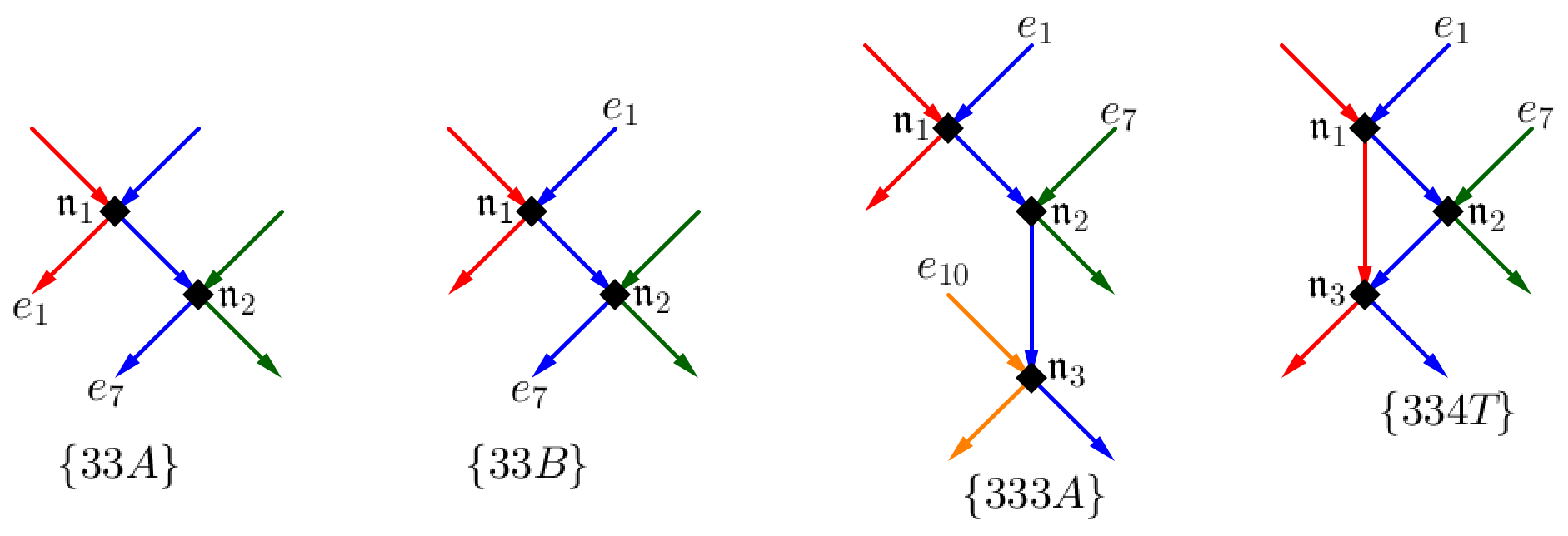
In fact, the algorithm tells us that, either we obtain one more {33A}-component other than the one with long bond (which is obviously sufficient), or we get a three-atom molecule that extends our long-bond {33A}-molecule, which has the form of either a {333A}-molecule or a {334T}-molecule, see Definition 2.6 and Figure 5. These molecules are extensions of the long-bond {33A}-molecule, in the sense that they contain one more collision which makes them more restrictive than the {33A}-molecule alone, leading to a better excess of (say) , which is sufficient for Theorem 1.
The proof for the {333A}- and {334T}-molecules are contained in Proposition 3.4. They are a bit involved but are still maganeable without computer assisted calculations.
1.4.2. The new algorithm
With the discussions in Section 1.4.1, we now describe our new algorithm that leads to the desired structure of elementary molecules. As discussed above, we would like to find a {33A}-molecule with a long bond; however this is not always possible, and there are cases where we need to find two separated {33A}-molecules (each with excess ) which also provides the same (or better) excess in dimensions . Note that this again does not match the goal in dimensions , suggesting that a refinement of the algorithm is needed in these cases.
First, we shall assume our molecule has a two-layer structure , see Proposition 4.14 for the precise description. This two-layer structure has significant similarity and difference with the UD-molecules which is fundamental in the molecular analysis in [26] (for example the and are not required to be forests here), but the key feature here is that any bond connecting an atom in and an atom in is a long bond. The reduction of Proposition 4.4 to Proposition 4.14 is an easy process, which involves the BFK theorem for short time (in order to obtain the long bonds), an induction argument on the number of particles to guarantee the connectedness of and , and a special argument involving {334T}-molecules (Lemma 4.13) that treats the case of a triangle with long bond. This proof is presented in Section 4.2.
Now, suppose as above. We start by choosing a highest atom in . Note that has two parent nodes in , and becomes deg 2 if both of them are cut; this can be guaranteed by the assumption that each particle line intersects both and , see Proposition 4.14. Suppose we choose the cutting sequence such that both are cut before , then we would get a long bond {33A}-molecule if the that is cut after the other has deg 3 when it is cut. To achieve this, a natural idea is to cut (or ) first, and proceed along a path connecting and in until reaching . A natural candicate of this path is the following: note that belongs to two particle lines, say and , where contains . Then we consider the first collision (which we call ) in that connects the two particles and (i.e. bring them to the same cluster). In this case, let be the particles (equivalently particle lines) that are connected to before , and let be the set of collisions among particles in before , see Proposition 4.15 for details. The natural path going from to is given by concatenating the paths from to in , and the path from to in .
We then have the following dichotomy, as shown in Proposition 4.15: either
-
(i)
one of the sets (say ) does not contain a recollision within it, or
-
(ii)
each set contains a recollision within it.
In fact, we will specify this recollision (i.e. cycle) to have a specific form called a canonical cycle, see Proposition 4.16.
In case (i), we can apply the plan stated above, where we start by cutting and follow the path from to in (cutting all atoms in in this process), and then follow the path from to in . The fact that does not contain a canonical cycle then implies that has deg 3 when it is cut, which leads to a {33A}-component with a long bond. This already guarentees excess by ; in order to improve this, we notice that contains many more recollisions other than the one provided by the {33A}-component (say ), and a simple argument suffices to show that either there exists another {33A}-component other than , or is contained in some {333A}- or {334T}-component. In each case the desired excess estimate follows from Propositions 3.3 and 3.4. For the detailed proof, see Proposition 4.16.
In case (ii), if we apply the same argument in case (i), then the atom would also have deg 2 when it is cut; this means that a {33A}-component occurs earlier in the cutting process, which may not contain a long bond. However, note that each contains a canonical cycle, which in particular implies that each contains a {33A}-component in a suitable cutting sequence. Since it is known that each {33A}-component (without long bond) provides excess , and that we only need to obtain excess in dimension (the case is much easier), we see that these two {33A}-components are already almost sufficient.
It remains to improve the excess a little bit upon . This is similar to case (i) but slightly more complicated; the idea is to locate a remaining atom that belongs to a particle line other than the ones in and . This atom is then cut as deg 3, and some subsequent atom will be cut as deg 2 (due to the many recollisions), leading to a third {33A}-component which provides the needed gain. This is contained in Proposition 4.17. Finally, if there is no such atom belonging to any “new” particle line, then either the canonical cycle is not a triangle (in which case an extra gain is possible, see the proof of Proposition 4.17), or the molecule has an essentially explicit form which contains exactly particle lines. In this last scenario, it is not hard to develop a specific cutting sequence (using the fact that we have exactly 6 particle lines) that guarantees at least three {33A}-molecules, which is again sufficient. This then finishes the proof of the excess estimate, which completes Theorem 1.
1.5. Plan for the rest of this paper
In Section 2 we summarize the relevant concepts and notations from [26], especially those related to molecules and cuttings, that are needed in this paper. In Section 3 we state and prove the integral and volume estimates needed in the torus case. These are similar to those in Section 9.1 in [26] but involve more complicated calculations. We also state Proposition 3.8, which is the main estimate proved in this paper, and the new ingredient that will come into the proof of Theorem 1. In Section 4 we prove Proposition 3.8 using the integral estimates in Section 3 and the full algorithm, which consists of the same arguments in Section 13.3 in [26] (see Section 4.1) and a new algorithm for the torus case (see Section 4.2). Finally, in Section 5 we prove Theorem 1. The proof mostly follows the same lines in [26] which is also sketched here; the new ingredients are the modifications in the algorithm due to double bonds (see Part 4), and the estimate for the term in [26] which relies on Proposition 3.8, see Part 6.
Acknowledgements
The authors are partly supported by a Simons Collaboration Grant on Wave Turbulence. The first author is supported in part by NSF grant DMS-2246908 and a Sloan Fellowship. The second author is supported in part by NSF grants DMS-1936640 and DMS-2350242. The authors would like to thank Isabelle Gallagher, Yan Guo, and Lingbing He for their helpful suggestions.
2. Summary of concepts from [26]
2.1. Molecules and associated notions
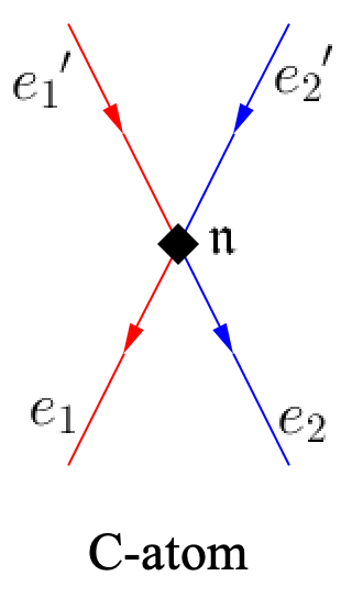
We recall the definition of molecules and some associated notions in [26]. Since the main proofs in the current paper (Sections 3–4) only requires molecules formed solely by C-atoms, we will only review the relevant definitions involving C-atoms here. For the full definitions involving both C- and O-atoms and empty ends etc., see Definitions 7.1–7.3 in [26].
Definition 2.1 (Molecules).
We define a (layered) molecule to be a structure , see Figure 3, which satisfies the following requirements.
-
(1)
Atoms, edges, bonds and ends. Assume is a set of nodes referred to as atoms, and is a set of edges consisting of bonds and ends to be specified below.
-
(a)
Each atom is marked as a C-atom, and is assigned with a unique layer which is a positive integer.
-
(b)
Each edge in is either a directed bond , which connects two distinct atoms , or a directed end, which is connected to one atom . Each end is either incoming or outgoing , and is also marked as either free or fixed.
-
(a)
-
(2)
Serial edges. The set specifies the particle line structure of (cf. Definition 2.2 (5)). More precisely, is a set of maps such that, for each atom , contains a bijective map from the set of 2 incoming edges at to the set of 2 outgoing edges at . Given an incoming edge and its image under this map, we say and are serial or on the same particle line at .
-
(3)
satisfies the following requirements.
-
(a)
Each atom has exactly 2 incoming and 2 outgoing edges.
-
(b)
There does not exist any closed directed path (which starts and ends at the same atom). Note that unlike the Euclidean case [26], double bonds are allowed in .
-
(c)
For any bond , we must have .
-
(a)
Definition 2.2 (More on molecules).
We define some related concepts for molecules.
-
(1)
Full molecules. If a molecule has no fixed end, we say is a full molecule.
-
(2)
Parents, children and descendants. Let be a molecule. If two atoms and are connected by a bond , then we say is a parent of , and is a child of . If is obtained from by iteratively taking parents, then we say is an ancestor of , and is a descendant of (this includes when ).
-
(3)
The partial ordering of nodes. We also define a partial ordering between all atoms, by defining if and only if and is a descendant of . In particular if is a child of . Using this partial ordering, we can define the lowest and highest atoms in a set of atoms, to be the minimal and maximal elements of under the partial ordering (such element need not be unique).
-
(4)
Top and bottom edges. We also refer to the incoming and outgoing edges as top and bottom edges.
- (5)
-
(6)
Sets and . Define to be the set of all bonds and free ends. Define also the sets (resp. ) to be the set of all ends (resp. all bottom ends).
-
(7)
Degree and other notions. Define the degree (abbreviated deg) of an atom to be the number of bonds and free ends at (i.e. not counting fixed ends). We also define to be the set of descendants of . Finally, for a subset , define , where where is the set of bonds between atoms in , and is the set of components of (where is viewed as a subgraph of ).
It is clear, with the definition of particle lines in (5), that each edge belongs to a unique particle line, and each particle line contains a unique bottom end and a unique top end, so the set of particle lines is in one-to-one correspondence with the set of bottom ends and also with the set of top ends.
In the next definition, we define the integral associated with a molecule . Note that for the purpose of this paper, the more relevant notion here is the in Definition 2.3 (4), which is the same as the one occurring in Section 9.1 in [26] (see also the in Proposition 8.10 in [26]), instead of the in Definition 7.3 in [26].
Definition 2.3 (The integral for molecules ).
Consider the molecule , we introduce the following definitions.
-
(1)
Associated variables and . We associate each node with a time variable and each edge with a position-velocity vector . We refer to them as associated variables and denote the collections of these variables by and .
-
(2)
Associated distributions . Given a C-atom , let and be are two bottom edges and top edges at respectively, such that and (resp. and ) are serial. We define the associated distribution by
(2.1) where is a unit vector, and .
-
(3)
The associated domain . The associated domain is defined by
(2.2) Here is a small parameter (for the exact choice see Section 5, Part 7).
-
(4)
The integral . Let be a molecule (which may or may not be full), with relevant notions as in Definitions 2.1–2.2, and be a given nonnegative function. We define the integral by
(2.3) Here in (2.3), and are the cardinalities of and with as in Definition 2.1 (note if is a full molecule), and is defined similar to in (1). We will assume that is supported in the set , with possibly other restrictions on its support to be specified below.
2.2. Cutting operations
We next recall the notion of cutting in [26]. Like in Section 2.1, we will only consider the case of cuttings involving C-atoms. For the full definition involving cutting both C- and O-atoms, see Definition 8.6 (and related properties in Section 8.2) in [26].
Definition 2.4.
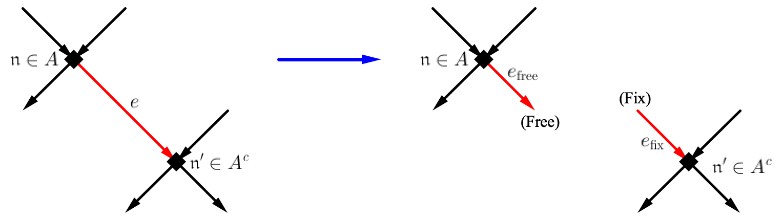
Let be a molecule formed solely by C-atoms and be a set of atoms. Define the operation of cutting as free, where for each bond between and is turned into a free end at and a fixed end at . Note that each free end formed after this cutting (at atoms in ) is uniquely paired with a fixed end formed after this cutting (an atoms in ), and this pair is associated with a unique bond before the cutting, see Figure 4 for an illustration. We also define cutting as fixed to be the same as cutting as free.
Given a molecule , we define a cutting sequence to be a sequence of cutting operations, each applied to the result of the previous cutting in the sequence, starting with . In considering cutting sequences below, we will adopt the following convention. Note that after cutting any as free or fixed from , the atom set of remains unchanged, but is divided into two disjoint molecules, with atom set and with atom set . Now depending on the context, we may tag as protected, in which case we will not touch anything in and will only work in in subsequent cuttings. Throughout this process we will abuse notations and replace by .
Next we define a natural linear ordering among all connected components of the resulting molecule after any cutting sequence, see Proposition 8.8 in [26].
Definition 2.5.
Let be a full molecule, and be the result of after any cutting sequence. Then, with , and the cutting sequence fixed, we can define an ordering between the components of :
-
(1)
If the first cutting in the sequence cuts into with atom set and with atom set , where is cut as free, then each component of with atom set contained in shall occur in the ordering before each component of with atom set contained in .
-
(2)
The ordering between the components with atom set contained in , and the ordering between the components with atom set contained in , are then determined inductively, by the cutting sequence after the first cutting.
Denote the above ordering by , where means occurs before in this ordering.
Finally we introduce the notion of elementary molecules (or components), see Definition 8.9 in [26]. However, here we only consider those formed solely by C-atoms; moreover, in view of the new estimates needed in the current paper, we need to extend the list of elementary molecules in [26] to include two new ones, namely the {333A}- and {334T}- molecules, see Definition 2.6 below.
Definition 2.6.
We define a molecule formed by C-atoms to be elementary, if it satisfies one of the followings:
-
(1)
This contains only one atom that has deg 2, 3 or 4; we further require that the two fixed ends are not serial, and are either both top or both bottom for C-atom.
-
(2)
This contains only two atoms connected by a bond, and their degs are either or .
-
(3)
This contains only three atoms, such that two of them have deg 3 and are connected by one bond, and the third atom either has deg 3 and is connected to one of them, or has deg 4 and is connecte to both of them.
For those in (1) and (2) we shall denote it by {2}-, {3}-, {4}-, {33}- and {44}-molecules in the obvious manner; for those in (3) we shall denote it by {333A}- or {334T}-molecules (where T stands for “triangle”). Moreover, for a {33}-molecule , we denote it by {33A} if we can cut one atom as free, such that the other atom has 2 fixed ends that are be both top or both bottom; otherwise denote it by {33B} (note that a {33} molecule is {33B} if and only if there is one top fixed end at the higher atom and one bottom fixed end at the lower atom). For {333A}- and {334T}-molecules, we also require that the first 2 atoms and form a {33A}-molecule with two fixed ends being both bottom or both top, and that the 2 fixed ends at the third atom , after cutting as free, must be both top or both bottom. For an illustration see Figure 5.
Suppose applying a cutting sequence to generates a number of elementary components, plus the rest of the molecule whose atoms are not cut by this cutting sequence, then we define and etc. to be the number of {2}- and {33}- etc. components generated in this cutting sequence. We also understand that, when any elementary component is generated in any cutting sequence, this component is automatically tagged as protected.
3. Treating the integral
3.1. Integrals for elementary molecules
In this subsection we recall the estimates in Section 9.1 in [26] concerning the integral (Definition 2.3) for elementary molecules ; in addition, we also prove some improvements of these estimates and some new estimates involving the new elementary molecules defined in the current paper. Throughout this section we will assume our molecules only consist of C-atoms; the case of O-atoms will have similar results with simpler proofs, and we will not elaborate on them.
Let be an elementary molecule as in Definition 2.6, and consider the integral
| (3.1) |
as defined in (2.3) in Definition 2.3 (4). Note that for fixed ends of , the variable is not integrated in (3.1) and acts as a parameter in this integral. The time variable at in (3.1) will be denoted by . When contains only one atom, we will also denote by ; when contains two (resp. three) atoms, we may also denote the edges by for (resp. ) depending on the context. The variable is then abbreviated as .
Remark 3.1.
Throughout this paper we will use to denote a large sonstant depending only on , and be any large quantity such that , where is a small constant depending only on . Below we always assume that the in (3.1) is nonnegative and supported in for each (thanks to the Maxwellian decay of the Boltzmann density (1.17)) and for each , where is a fixed integer for each . We may make other restrictions on the support of , which will be discussed below depending on different scenarios; such support may also depend on some other external parameters such as , which will be clearly indicated when they occur below.
Proposition 3.2.
Let be defined as in (3.1), where contains only one atom.
-
(1)
If is a {2}-molecule as in Definition 2.6, i.e. the two fixed ends are either both bottom or both top, by symmetry we may assume are fixed and are free. Then we have
(3.2) Here in (3.2), the summation is taken over the (discrete) set of that satisfies the following equation:
(3.3) where is a unit vector. Moreover is the same function in (3.1) with input variables , where (each choice of) is a function of defined above, and is also some function of , which is defined via (1.4) conjugated by the free transport .
Note that all the values of occurring in the summation in (3.2) can be indexed by a variable with , which represents different fundamental domains of within . The number of choices of is , and this allows to decompose
(3.4) where for each , the variables in in (3.4) is defined as above with being the solution to (3.2) indexed by .
-
(2)
If is a {3}-molecule as in Definition 2.6, by symmetry we may assume is fixed and are free. Then
(3.5) Here in (3.5) the input variables of are , where (similar to (1.4))
(3.6) In the integral (3.6) the domain of integration can be restricted to and , which has volume . The same logarithmic upper bound also holds for the weight .
In addition, assume is supported in some set depending on some external parameters , and the support satisfies
(3.7) for some , where in the first case in (3.7) and in the second case. Then in each case, the domain of integration in (3.5) can be restricted to a set of that depends on and the external parameters, which has volume .
-
(3)
If is a {4}-molecule as in Definition 2.6, and we still consider the same in (3.1), then
(3.8) where the inputs of are as in (3.6). In the integral (3.8) the domain of integration can be restricted to and , which has volume . The same logarithmic upper bound also holds for the weight .
In addition, assume is supported in the set (depending on some external parameters )
(3.9) for some and , then in this case, the domain of integration in (3.8) can be restricted to a set of that depends on the external parameters, which has volume .
-
(4)
In (2) and (3) above, suppose we do not assume (3.7) or (3.9). Instead, we assume that is supported in the set where, for the vectors and with some , there exist at least two different values such that the equality (3.3) holds. Then, we can restrict the domain of integration in (3.5) (and (3.8)) to a set of that depends on (or a set of ) which has volume .
- (5)
-
(6)
In (2) above, suppose we do not assume (3.7). Instead, we assume that is supported in the set (depending on some external parameters )
(3.10) for some and , and for some . Then the domain of integration in (3.5) can be restricted to a set of that depends on and the external parameters, which has volume .
Proof.
(1) By (3.1), we have
| (3.11) |
By fixing some representative of we may assume , then we have
| (3.12) |
where is the norm in . Inserting into (2.1), we get
| (3.13) |
| (3.14) | ||||
Therefore, we have the same decomposition for :
| (3.15) |
where follows from the bound of and in the integral , and is given by
| (3.16) |
Now note that is exactly the same as the in [26], up to translation by , see equations (7.1) and (9.1) in [26]. By Proposition 9.1 (1) in [26], we get
| (3.17) |
(2) Note that is fixed, and , so by our convention (see Section 1.2.1) we can identify the vector with its unique representative that has Euclidean length . Then we can introduce the variable such that , and make the change of variable , just as in the proof of Proposition 9.1 (2) in [26]. We carefully note that this substitution changes the integral in to the integral in , without introducing the fundamental domain decomposition (3.4). The rest of the proof then follows the same arguments as in Proposition 9.1 (2) in [26], which leads to (3.5)–(3.6).
The proof of the extra volume bound under the assumption (3.7) also follows from similar arguments as in Proposition 9.1 (2) in [26]; if is supported in or or , then we already gain this factor from the or integral in (3.5); if is supported in (or which is similar) then we get . By making the fundamental domain decomposition (3.4) and dyadic decompositions for (or ), and gaining from both the and integrals in (3.5), we get the desired volume bound .
(3) This follows from the proof of (2) by adding the extra integrations in and .
(4) The two conclusions here are related to (2) and (3) respectively. We only prove the one related to (2), as the other one follows by adding the extra integrations in and .
By (3.5), we get
| (3.18) |
and we need to show that belongs to a set of volume . The assumption on the support of implies that in the set of , there must exist such that for some , we have
| (3.19) |
Moreover, since we must also have in (3.19), as under the assumption (or ), there exists at most one solution to (3.19) with fixed .
Now, from (3.19) we deduce that
| (3.20) |
Note that is a nonzero integer vector (which we may fix up to a loss). If then (3.20) obviously restricts (and thus restricts with fixed ) to a set of volume . If , then is restricted to a set of volume , and so is (with fixed ) as is the reflection of with respect to the orthogonal plane of , and this reflection preserves volume. This allows us to bound the volume of the set of by for each fixed , which proves (4).
(5) By the same arguments as in (4), from the assumptions on the support of we obtain that
| (3.21) |
for some nonzero integer vectors and . From the inequality for , we already know that (and hence with fixed ) belongs to a set of volume . Moreover, using the inequality for , and the fact that is the reflection of with respect to the orthogonal plane of , we get that
| (3.22) |
Note also that by the first inequality in (3.20) (with ), we conclude that for fixed values of and , the condition (3.22) restricts to a subset of of volume . In fact, let and be the unit vector in the directions of and respectively, then (3.20) implies that , and thus and for any vector . The desired volume bound then follows from the first inequality if and from the second inequality if .
By putting together the volume bound for which is independent of , and the volume bound for with fixed , we have proved (5).
(6) We know and is supported in the set where (3.10) holds. From (3.10), and using also that due to the collision, it follows that, after shifting the fundamental domain by some which we may fix at a loss of , we get (note that )
| (3.23) |
Let , then (3.23) implies that
| (3.24) |
where and is a constant 2-form depending only on . By a dyadic decomposition we may assume for some dyadic (or if , or if ). Note that for fixed , the inequality (3.24) restricts to a tube in with size in one direction and size in all other directions; let this tube by . Denote also , then (corresponding to respectively).
We first claim that: for fixed (hence fixed ), the condition restricts to a subset of with measure (of course, with fixed, is then restricted to a set of the same measure). In fact, if this is trivial using the volume of . If , for fixed we can represent by the new coordinates and (where is the plane orthogonal to ). Denote also . If , then by a simple Jacobian calculation, we see that the restriction implies that belongs to a set whose measure is bounded by
with the verification of the last inequality being straightforward (the choice of only increases the volume by a factor ). Finally, if and dimension , then the same argument applies with replaced by which is the rotation of ; if and dimension , we may first fix and , then , and it is easy to see that the measure of the two dimensional set is bounded by . This proves the first claim in either case.
We next claim that: for fixed , the condition restricts to a subset of with measure . In fact, recall . if , then the desired bound follows by solving a linear inequality in ; if . then by the assumption , we know that , and hence , in which case the desired bound becomes obvious (the set of is trivially bounded by ). This proves the second claim.
By putting the above two claims together (and summing over which loses at most a logarithm and can be absorbed by ), we then conclude that belongs to a set of volume
which proves (6). ∎
Proposition 3.3.
Consider the same setting as in Proposition 3.2, but now is an elementary molecule with two atoms , where is a parent of , which satisfies one of the following assumptions:
-
(a)
Suppose is a {33A}-molecule with atoms . Let be the two fixed ends at and respectively. Assume that either (i) for the two atoms and , or (ii) is supported in the set
(3.25) for some , where as above.
-
(b)
Suppose is a {33B}-molecule. Assume that is supported in the set
(3.26) for some , where again .
-
(c)
Suppose is a {44}-molecule with atoms and being two free ends at and respectively, such that becomes a {33A}-molecule after turning these two free ends into fixed ends. Moreover assume that is supported in the set (where )
(3.27)
Then, in any of the above cases, we can decompose (similar to (3.4)) that , such that for each , we have
| (3.28) |
Here and (in fact in cases b and c) are opens set in some , and depends on for fixed ends while does not, and the input variables of are explicit functions of and for fixed ends . We also have (which is true in case a even without assuming (i) or (ii)). As for , we have the folowing estimates:
Proof.
First note that the statements other than (1)–(5) are obvious. For example, the decomposition can be proved by inserting (3.12) into the expression of . The construction of such that is the same as the proof of Proposition 9.2 in [26]. Below we focus on the proof of (1)–(5). Also we may fix one choice of the fundamental domain , but by a suitable shift (similar to the proof of Proposition 3.2) we can omit this and work on .
(1) To calculate , we first fix the values of and all for edges at , and integrate in and all for all the free ends at . By assumption, we know that becomes a deg 2 atom with two top fixed ends after cutting as free. Let the inner integral be , then we can apply (3.2) in Proposition 3.2 to get an explicit expression of .
Let the bond between and be , denote the edges at by as in Proposition 3.2, then for some . After plugging in the above formula for the inner integral , we can reduce by an integral of form as described in (2) of Proposition 3.2, namely
| (3.29) |
where the input variables of are explicit functions of and using Proposition 3.2 and the fact that satisfies (3.6).
Note that the integral (3.29) has the same form as (3.5) in Proposition 3.2 (2) and (6), and the indicator function restricts to a set which satisfies (3.10) in Proposition 3.2 6). with replaced by . Then, by the same argument as in the proof of Proposition 3.2 6), we can define and assume , such that for fixed (hence fixed ) the volume of the set of is bounded by .
Suppose , by assmption (i) in case (a), we know that for some fixed value (which is either or ), so belongs to an interval of length , which leads to the first upper bound for the volume of the set of , namely .
On the other hand, by assumption we have
| (3.30) |
By taking a linear combination, this implies that , which means that (and hence ) belongs to a fixed ball of radius . By the same proof as in Proposition 3.2 6), we know that this restricts to a set with volume , which is the second upper bound on the volume of the set of .
Summing up, we then know that is restricted to a set whose volume is bounded by
which proves (1).
(2) In this case, all the discussions leading to (3.29) are the same as in (1), and the inequality (3.10) is also the same as in (1), with replaced by . Moreover, we also have , so by directly applying Proposition 3.2 (6), we get that is restricted to a set whose volume is bounded by . This proves (2).
(3) We adopt the same notations for etc. as in (1), which again leads to (3.29) as in (1) and (2). Now using the condition , we will perform a different change of coordinates. Define , and , then from (3.29) we have
| (3.31) |
where the values of are determined by the fixed ends and the values of , and is the indicator function that the two particles with state and collide. To prove (3), it suffices to show that
| (3.32) |
where all the conditions on the support of are imposed in the integral in (3.32) without explicit mentioning (same below). Here, if necessary, we may perform a dyadic decomposition on the size of to replace it by a constant in order to match the form (3.28); this leads to at most logarithmic loss which can be absorbed into .
Note that the function depends on , and depending on the cases of . By using polar coordinates in and a simple Jacobian calculation, we have
| (3.33) |
where is the plane orthogonal to and is the Hausdorff measure on that plane. Below, if (so ), we shall keep the in (3.31); if (so ), we shall substitute by (3.33). One easy case is when ; this implies either or . In either case, note that dimension , we can prove (3.32) by direct integration in and , by using (3.33) and exploiting the symmetry between and if necessary.
Next we will assume and analyze the factor . In the support of this factor, there exists unique such that
| (3.34) |
where depending on whether or , and . We would like to substitute the variable by ; indeed, using equations (7.1) and (7.10) in [26], we have
| (3.35) |
where is as in (3.34). Now, using polar coordinates in the vector
we can rewrite the function in (3.35) as the two Dirac function and (which leads to integration in ). In this way, we get the following upper bounds for (3.32):
-
•
If , then we directly get
(3.36) - •
-
•
If , then in (3.34), which complicates things a bit. In this case we have
(3.38) and note that by our assumption. Now we use the second expression in (3.33), and write
Note that the function is comparable to the Hausdorff measure on the cone . We denote this cone (or two rays if ) by and its Huausdorff measure by , which is bounded on bounded sets. This leads to
(3.39) - •
Now we are ready to prove (3.32). In fact, we may fix and . The integral in in (3.36) and the integral in in (3.40) is trivially bounded by . As for the integral in , since , we only need to worry about the denominator in (3.40). However the numerator , and the term cancels the denominator; as for the factor, note that is given by (3.38) (and the same for when ), so the cancels the coefficient before and yields
(for example, we may perform a dyadic decomposition in and use that the measure for the set of satisfying is bounded by ). This proves (3.32).
(4) This is the same as Proposition 9.2 (2) in [26]. The proof is tedious and not much related to the rest of this paper, so we omit it here and refer the reader to [26].
(5) Note that, if we fix the variables , then essentially reduces to the same integral expression but for a {33A}-molecule. Therefore, by adding the extra integration over in (3.29), we get
| (3.41) |
According to the support assmption of in (3.27), we know that
This then proves (5), by noticing that and . ∎
Proposition 3.4.
Consider the same setting as in Proposition 3.2, but now is an elementary molecule with three atoms as in Definition 2.6, where is a parent of , which satisfies one of the following assumptions:
-
(1)
Suppose is a {333A}-molecule with atoms . Let and be the three fixed ends at respectively. Assume is supported in the set that
(3.42) for some , and that
(3.43) for the same as above, where .
-
(2)
Suppose is a {334T}-molecule with atoms . Let and be the two fixed ends at and respectively. Assume is supported in the set that
(3.44) for some , and that
(3.45) for the same as above, where .
Then in each case, we can decompose (similar to (3.4)) that , such that for each , we have
| (3.46) |
Here the and are as in Proposition 3.3 (so depends on for fixed ends while does not, etc.), except that the estimate for should be replaced by .
Proof.
For {333A}-molecules, at the expense of a factor of at most , we can bound each single individually, which allows us to lift to the Euclidean covering and assume that the spatial domain is . For {334T}-molecules, we can still do this for the two atoms which forms the {33A}-molecule. We adopt the same convention regarding etc. as in Proposition 3.3; in particular we assume has collision with at atom with . Moreover, we can distinguish three cases:
-
(a)
When is {333A}-molecule with adjacent with ; in this case we define (with and and associated ) to be the bond between and , where is serial with and is not.
-
(b)
When is {334T}-molecule; in this case we define (with ) as in (a), and define (with ) to be the bond between and . Note that .
-
(c)
When is {333A}-molecule with adjacent with ; in this case we define (with ) as in (b).
Arguing as in the proof of Proposition 3.3 (3), we only need to prove that
| (3.47) |
where . The second indicator function equals in case (a), and in case (b), and in case (c). We may assume , otherwise (3.47) is trivial. Note that we have by either (3.43) or (3.45); using also (3.34), this implies that . Now, following the same arguments as in the proof of Proposition 3.3 (3) (i.e. analyzing the {33A}-molecule formed by and ), we get the following expression (corresponding to (3.40)):
| (3.48) |
where either and , or and , with the relvant notations same as in the proof of Proposition 3.3 (3). Now we consider the three different cases.
-
•
Case (a) ({333A}-molecule with connected to ). In this case we have that is fixed. We will fix in (3.48) (i.e. integrate it after all the other variables) and control the measure of the set of (note that , also the integral is uniformly bounded). The factor implies that there exists such that
(3.49) which combined with the fact that (due to the collision ) gives that
(3.50) Denote , then we have . Note also that
corresponding to , and that . This implies that up to , where
(3.51) Note that by (3.34) and (3.43) we have
Let for some dyadic , then belongs to an interval of length since . Moreover, with fixed, by the inequality , we know the given by (3.51) belongs to a tube of size in one dimension and in all other dimensions. With and fixed, the value of is also fixed (up to perturbation ) as in (3.38). Note that the defined by (3.51) belongs to a sphere of radius which is parametrized by . The intersection of the tube with this sphere equals a subset of the sphere with diameter , which implies that belongs to a set of measure . Putting together the above estimates for and , we have proved (3.47). Note the order of integration here is: , then , then , then .
-
•
Case (b) ({334T}-molecule). This case is similar to (a), except that collides with instead of . We shall fix and control the measure of the set of . Let for some dyadic , then , so belongs to an interval of length . Now we fix . This also fixes and we have . Note that both and the set depend on , but with fixed , the can be mapped to some at a uniformly bounded Jacobian, and the variable belongs to a set which is independent of , so we are allowed to integrate in with fixed . Then and are both fixed up to error .
Now we can repeat the discussion in (a) with in place of . Note that now in comparison with (a); moreover, the in (a) should be replaced by which equals where depends only on and , so if as in (a) then belongs to a set of measure with and fixed. Finally, with fixed, the same proof in (a) yields that belongs to a set of measure . Putting together the above estimates for and and , we have proved (3.47). The order of integration here: , then (mapped from ), then , then .
-
•
Case (c) ({333A}-molecule with connected to ). In this case, we have that collides with . We shall fix and control the measure of the set of . By the same calculation as above, we get , where now . Let , then belongs to an interval of length . Now we fix so is also fixed. Then (and hence belongs to a fixed tube (similar to (a) and (b) above) in the direction of , which has thickness in the orthogonal direction of . On the other hand, with fixed, we know that belongs to which is close to (and is integrated according to the corresponding Hausdorff measure) where . Let for some dyadic , then with fixed, this forces to belong to a set in of measure . Finally, if , then we have
It is then easy to see that (if not, then also, hence , contradicting (3.43)), and thus with fixed, must belong to an interval of length . Putting together all the above estimates for , and , we have proved (3.47). The order of integration here: , then , then , then .∎
3.2. Definition of excess
Suppose is reduced to that contains only elementary components, after certain cutting sequence. By the same discussion in Section 9.3 in [26], we may put certain restrictions on the support of the function occurring in (2.3) (and also (3.1)), by inserting certain indicator functions that form a partition of unity. If such a indicator function is fixed, we may then say that the integral (2.3) (or (3.1)) is restricted to a certain set, which is specified by indicator function.
Now we recall the definition of good, normal and bad components of , see Definition 9.5 in [26]. In the current paper, we will need an extension of these definitions, as well as a more quantitative description of the gain for each good component, in the form of excess in Definition 3.6 below. Note that these definitions depend on both the structure of , and also the restrictions (i.e. support conditions of ), hence they depend on the specific choice of the indicator functions described above.
Definition 3.5.
The following components are normal:
The following components are bad:
-
(4)
Any {4}-component, except those described in (9) below.
The following components are good:
-
(5)
Any {3}-component , which occurs in some restriction in the following sense. The integral (3.1) is restricted to the set where one of the following two assumptions hold:
(3.52) (3.53) Here in (3.52) we assume that (i) are two different ends at ; (ii) is a free end at , while is an atom in a component with in the sense of Definition 2.5, and is a free end or bond at . In (3.53) we assume that are two different ends at which are both bottom or both top. Note that if (or ) is the fixed end, then equals where is the free end paired with in the sense of Definition 2.4, so (3.52) can still be expressed as a condition of ; same with (6)–(9) below.
- (6)
-
(7)
Any {33B}-component , and the integral (3.1) is restricted to the set where
(3.55) for any two distinct edges at the same atom.
-
(8)
Any {44}-component , and the integral (3.1) is restricted to the set where
(3.56) where are two free ends at and respectively, such that becomes a {33A}-molecule after turning these two free ends into fixed ends.
- (9)
Definition 3.6.
Let be any elementary molecule as in Definition 2.6; note that here we are allowed to add various restrictions to the support of as in Propositions 3.2–3.4. Let be as in (3.1). For dyadic number , we say has excess , if (or each component of as in Proposition 3.3) can be bounded by an integral of form (3.28), i.e.
| (3.59) |
Here the and are as in Proposition 3.3 (so depends on for fixed ends and possibly on the external parameters while does not, etc.), except that the estimate for should be replaced by
| (3.60) |
If is a good {4}-molecule, then the inequality (3.60) should be replaced by (cf. (3.8))
| (3.61) |
Proposition 3.7.
The following results are true:
-
(1)
If is a good component in the sense of Definition 3.5, then it has excess .
-
(2)
If is a {3}- or {4}-component as in Proposition 3.2 (2) and (3) that satisfies either (3.7) or (3.9) with some , then has excess . If is a {3}- or {4}-component as in in Proposition 3.2 (4), then has excess . If is a {4}-component as in Proposition 3.2 (5), then has excess . If is a {3}-component as in Proposition 3.2 (6) that satisfies (3.10) and with some , then has excess .
- (3)
- (4)
3.3. The main combinatorial proposition
Now we can finally state the main technical (combinatorial) ingredient of the current paper, namely Proposition 3.8 below. This proposition plays the role of Proposition 13.1 in [26], and is in fact a refinement of the latter with the extra proofs needed in the torus case. It is also a major component of the proof of Theorem 1 in Section 5, see Part 6 in Section 5.
Proposition 3.8.
Let be a large absolute constant depending only on the dimension . Let be a full molecule of C-atoms with all atoms in the same layer (see Definition 2.1 for layers), such that all its bonds form a tree of atoms plus exactly bonds where .
Then there exists a cutting sequence that cuts into elementary components (Definition 2.6), such that (after decomposing 1 into at most indicator functions, where is the set of atoms of ) one of the followings happen:
-
(1)
There is at least one good {44}-component, and also .
-
(2)
All {33B}- and {44}- components are good, and
(3.62) -
(3)
There is exactly one {4}-component, and all the other components are {2}-, {3}-, {33A}-, {333A}- and {334T}-components. Moreover there exists at most 10 components, each having excess as in Definition 3.6, such that .
4. Proof of Proposition 3.8
From now on we focus on the proof of Proposition 3.8. We start by recalling the basic algorithm UP in [26] and its properties (Definition 10.1 and Proposition 10.2 in [26]).
Definition 4.1 (The algorithm UP).
Define the following cutting algorithm UP. It takes as input any molecule of C-atoms which has no top fixed end. For any such , define the cutting sequence as follows:
-
(1)
If contains any deg atom , then cut it as free, and repeat until there is no deg atom left.
-
(2)
Choose a lowest atom in the set of all deg 3 atoms in (or a lowest atom in , if only contains deg 4 atoms). Let be the set of descendants of (Definition 2.2).
- (3)
We also define the dual algorithm DOWN, by reversing the notions of parent/child, lowest/highest, top/bottom etc. It applies to any molecule of C-atoms that has no bottom fixed end.
Proposition 4.2.
Let be any connected molecule as in Definition 4.1. Then after applying algorithm UP to (and same for DOWN), it becomes which contains only elementary components. Moreover, among these elementary components:
-
(1)
We have and , and if and only if is full. If has no deg atom, and either contains a cycle or contains at least two deg atoms, then either or contains a good component (in the sense of Definition 3.5). If has no deg 2 atom and at most one deg 3 atom, and is also a tree, then contains (at most one) {4}-component and others are all {3}-components.
-
(2)
If has no deg 2 atom and at most one deg 3 atom, and contains a cycle, then we can decompose 1 into indicator functions, such that for each indicator function, must contain a good component (possibly after cutting the {33A}-component into a {3}- and a {2}-component).
Proof.
(1) The proof is basically the same as Proposition 10.2 in [26]. The only adjustment needed is due to the possibility of having double bonds, which only affects the part of the proof involving {33A}-components.
More precisely, assuming has no deg atom, and either contains a cycle or contains at least two deg atoms, we need to prove that has one {33A}- or good component. Suppose not, then we will show that also cannot contain any {2}-component; this would then lead to a contradiction by repeating the same proof of Proposition 10.2 in [26].
Now assume has a {2}-component, let the first atom that has deg 2 when we cut it, and consider the cutting operation that turns into deg 2, which must be cutting some atom as free. This cutting creates a fixed end at , so by Definition 2.4, this must be a parent or child of . At the time of cutting , if has deg 3, then must also have deg 3, which violates Definition 4.1 (3). Therefore the operation of cutting must turn the deg 4 atom into deg 2. This means that
-
•
and are connected by a double bond.
However, with , it is easy to see that for the two bonds connecting and (which are both bottom or both top), and the corresponding vectors and , there must exist two different values that satisfy the equality (3.3). Since is a {3}- or {4}-component in , we know that it must be a good component due to Definition 3.5 (5) or (9) (i.e. (3.53) or (3.58)), which leads to a contradiction.
(2) The proof is basically the same as Proposition 10.2 in [26], with the same adjustments made as in (1) above in the case of double bonds. We omit the details. ∎
Next, we recall the notions of strong and weak degeneracies (Propositions 10.5 and 10.16 in [26]), and properness and primitivity (Definition 8.2 and Proposition 10.4 in [26]).
Definition 4.3.
We define the following notions.
-
(1)
Strong degeneracy. Define a pair of atoms to be strongly degenerate if they are adjacent, and there exist edges at and respectively, such that cutting as free in and turning into fixed ends results in a {33A}-component, and we have the restriction (by indicator functions) that and .
-
(2)
Weak degeneracy. Define the atom pair to be weakly degenerate if they are adjacent, and we have the restriction (by indicator functions) that . Define also one atom to be weakly degenerate if we have the restriction for two distinct edges at .
-
(3)
Primitivity. Define an atom pair in to be primitive if is a parent of (but they are not connectedby a double bond), and the other parent of is not a descendant of .
-
(4)
Properness. Define a molecule to be proper, if it is a forest, contains only deg 3 and 4 atoms, with the distance (i.e. length of shortest undirected path) between any two deg 3 atoms being at least 3.
4.1. The cutting algorithm: general case
A major part of the proof of Proposition 3.8 is the same as in Section 13.3 in [26], but the torus case involves one new difficulty, namely that the number of collisions between a fixed number of particles now has no absolute upper bound, unlike the Euclidean case due to [16]. This difficulty then requires one new ingredient, which is treated in Proposition 4.1 below.
Proposition 4.4.
Define the function
| (4.1) |
for positive integers . Suppose satisfies the following properties:
-
(1)
is a full molecule, has at most bottom free ends and at least atoms;
-
(2)
does not contain double bonds;
-
(3)
does not contain any strongly degenerate primitive pair as defined in Definition 4.3;
Then, for this , there exists a cutting sequence such that Proposition 3.8 (3) holds true.
The proof of Proposition 4.1 is contained in Section 4.2 below. In the rest of this subsection we shall prove Proposition 3.8 under the assumption of Proposition 4.1. The proof is essentially the same as in Section 13.3 in [26]; for the reader’s convenience we still include it here.
Definition 4.5.
Let be a full molecule of C-atoms, and is an atom set. We say is transversal, if we can decompose into two disjoint subsets and , such that no atom in is parent of any atom in , and no atom in is parent of any atom in .
For any transversal set , define the set such that, an atom if and only if and has two bonds connected to two atoms in . Then define the set inductively as follows: an atom if and only if and has two bonds connected to two atoms in .
Proposition 4.6.
Let be a connected transversal subset and is a connected molecule.
-
(1)
We can always choose in Definition 4.5 such that each component of has at least one bond connected to .
-
(2)
Let and , then if and only if and has two children (or two parents) in . Similarly, the sets can be defined in the same way as , but with the sentence “ has two bonds connected to two atoms in ” replaced by “ has two children (or two parents) in ”.
-
(3)
The set is also connected and transversal. Moreover any atom in has at most one bond with atoms in , so .
-
(4)
Recall defined in Definition 2.2. Then there exists a connected transversal set , such that , and either or .
Proof.
(1) Suppose has a component that is not connected to by a bond, then we replace by and by , which still satisfies the requirements for in Definition 4.5, but the number of components of decreases by . Repeat until component of is connected to by a bond (or becomes empty).
(2) If an atom belongs to , then must have two children (or two parents) in . Now suppose has two adjacent atoms and in . If belongs to , then must be a parent (or child) of , and the same holds for . This means that either both and both are children of (so ), or both and both are parents of . Repeating this discussion, we get the desired splitting .
(3) Connectedness is obvious by definition. To prove transversality, we simply decompose , where and . This then satisfies the requirements (using the fact that any child (or parent) of any atom must belong to ). The second statement follows from the definition of in Definition 4.5.
(4) Suppose is connected and transversal; we may assume and (otherwise choose ). Since is connected, there must exist an atom that is either a parent or child of an atom in . We may assume it is a parent, and then choose a lowest atom among these parents. Since , we know that has only one bond with atoms in ; let , then is connected and .
Now we claim that is transversal. To see this, define to be the set of atoms that are descendants of , and decompose , where and . Clearly no atom in can be parent of any atom in , and no atom in can be parent of any atom in . If an atom is parent of some atom , then , but and is child of , so we also have , contradiction. Finally if is parent of , clearly , but then is also parent of an atom in , contradicting the lowest assumption of .
Now we know that is also connected transversal; replacing by and repeating the above discussion, we eventually will reach some such that either or , as desired. ∎
Definition 4.7 (Algorithm TRANSUP).
Suppose is connected full molecule and is a connected transversal subset. We may choose as in Proposition 4.6 (1). Define the following algorithm:
-
(1)
If contains any deg atom , then cut it as free, and repeat until there is no deg atom left.
-
(2)
Choose a lowest atom in the set of all deg 3 atoms in (or a lowest atom in , if only contains deg 4 atoms). Let be the set of descendants of in .
-
(3)
Starting from , choose a highest atom in that has not been cut. If has deg 3, and is adjacent to an atom that also has deg 3, then cut as free; otherwise cut as free. Repeat until all atoms in have been cut. Then go to (1).
- (4)
We also define the dual algorithm TRANSDN by reversing the notions of parent/child etc. Note that we replace and by and , and also replace by in Proposition 4.6 (1).
Proposition 4.8.
Suppose has no double bond. For the algorithm TRANSUP (and same for TRANSDN), we have and , and .
Proof.
It is clear, in the same way as in the proof of Proposition 4.2, that during the process, there is no top fixed end in or in , and there is no bottom fixed end in or in , so . Moreover because no component of the remaining part of after Definition 4.7 (3) can be full when it is first cut in Definition 4.7 (4) (thanks to Proposition 4.6 (1)), and no component of can be full when it is first cut in Definition 4.7 (4) (thanks to being connected).
To prove the lower bound for , note that only one atom in belongs to a {4}-component (as is connected). Let the number of atoms in that belongs to a {2}-component be , then by using the invariance of during cutting operations on (where is the set of all free ends and bonds at atoms in , including in all the elementary components), we deduce that . To see this, just note that initially is and is finally . Then, for each , which is connected to two atoms by two bonds, assume say is cut after . The total number of such is at least as each can be obtained from at most two . For each such , the corresponding must have deg 3 when it is cut, so by Definition 4.7 (3), it must belong to either {4}-, or {2}-, or {33A}-component. Using the upper bound for the number of {4}- and {2}-components, this completes the proof. ∎
Definition 4.9 (The function SELECT2).
Let be a connected molecule with only C-atoms, no bottom fixed end, and no deg 2 atoms. Let be the set of deg 3 atoms in , and let be a subset of atoms in such that becomes a forest after removing the atoms in . We define the function as follows.
-
(1)
Consider all the components of in , which is a finite collection of disjoint subsets of .
-
(2)
If any two of the subsets in (1), say and , have the shortest distance (within ) which is at most 4, then we choose one shortest path between an atom in and an atom in , and let the atoms on this path be . Then replace the two sets and by a single set which is .
-
(3)
Repeat (2) until this can no longer be done. Next, if a single subset contains two atoms (which may be the same) that are connected by a path of length at most 4 with none of the intermediate atoms belonging to or any other subset, then add the atoms on this path to . If this causes the shortest distance between two subsets to be , then proceed to (2) and repeat it as above.
- (4)
Proposition 4.10.
The molecule becomes a proper forest after cutting as free, and we also have .
Proof.
First becomes a forest after cutting as free, because . Assume is not proper (Definition 4.3) after cutting as free, say there exist two deg 3 atoms and of distance at most . As , we know and must both have deg 4 in , thus each of them must be adjacent to an atom in , say and , so the distance betwewn and is at most . Now consider the sets in Definition 4.9 (4) that form . If and belong to two different sets among them, then we get a contradiction with the absence of the scenario in Definition 4.9 (2); if and belong to the same set among them, then we get a contradiction with the absence of the scenario in Definition 4.9 (3).
In summary, we know is a proper forest after cutting as free. As for the upper bound for , simply note that each single step in Definition 4.9 (2)–(3) adds at most atoms to . Moreover each single step in Definition 4.9 (2) decreases the number of subsets by 1 and does not decrease , while each single step in Definition 4.9 (3) does not change the number of subsets, but adds one more cycle to . In particular adding this cycle increases the value of by at least 1, while we always have because , so the number of steps in Definition 4.9 (3) is bounded by a constant multiple of , hence the result. ∎
Definition 4.11 (Algorithm MAINTRUP).
Suppose is a connected full molecule and is a connected transversal subset. We may choose as in Proposition 4.6 (1). Let the number of bonds connecting an atom in to an atom in be . It is easy to prove that there exists a set of at most atoms, such that becomes a forest after cutting atoms in as free. Moreover, by decomposing 1 into at most indicator functions, we can identify a set of weakly degenerate atoms and atom pairs in in the sense of Definition 4.3; let be the atoms involved in these weak degeneracies. We define the following algorithm, which contains two Options that we can choose at the beginning.
In Option 1 we do the followings:
-
(1)
Cut as free, then cut it into elementary components using UP.
-
(2)
Then cut as free and cut it into elementary components using UP, then cut into elementary components using DOWN.
In Option 2 we do the followings:
-
(1)
Cut all atoms in as free. If any atom in becomes deg 2, also cut it as free until has no deg 2 atom.
-
(2)
If remains connected after the above step, let be the set of deg 3 atoms in , and be those atoms in that have not been cut. Define as in Definition 4.9, then cut as free and cut it into elementary components using DOWN. If is not connected, apply this step to each connected component of .
-
(3)
If not all atoms in have been cut, then choose a lowest atom in that has not been cut. If is adjacent to an atom that has deg 3, then cut as free; otherwise cut as free.
-
(4)
If any two deg 3 atoms in becomes adjacent, then cut as free. Repeat until no such instances exist.
-
(5)
If the distance of any two deg 3 atoms in becomes 2, say and are both adjacent to some , then cut as free and then cut as free from . Go to (4). Repeat until becomes proper again.
-
(6)
Repeat (3) until all atoms in have been cut. Then choose any deg 3 atom in and cut it as free. If the distance between any two deg 3 atoms in becomes at most 2, go to (4) and repeat (4)–(5) until becomes proper again. Then choose the next deg 3 atom in and cut it as free, and repeat until all atoms in have been cut.
-
(7)
Finally, cut (the remaining parts of) as free and cut it into elementary components using UP, and then cut into elementary components using DOWN.
We define the dual algorithm MAINTRDN in the same way (so is replaced by etc.).
Proposition 4.12.
Proof.
The case of Option 1 is easy; is obvious by definition, and because is connected and satisfies the assumption in Proposition 4.6 (1), in the same way as in the proof of Proposition 4.8. Moreover, each atom in belongs to a {4}- or {3}- or {2}- or {33A}-component, and the total number of {2}- and {33A}-components is equal to . For any atom that belongs to a {3}-component, if it is a weakly degenerate atom, or if it is part of a weakly degenerate pair and is cut after the other atom of the pair, then must be a good component by Definition 3.5 (5). This gives at least good components, as desired.
In the case of Option 2, note that in the whole process, there is no top fixed end in and no bottom fixed end in ; this is because for the lowest atom in chosen in Definition 4.11 (3), any child of must either belong to or belong to (and thus will have already been cut). Moreover, any chosen in this step either has deg 2 and no bond connecting to or has deg 3 and exactly one bond connecting to (because all atoms in have been cut in Definition 4.11 (1)). Also any {33}-component cut in this way must be {33A}-component, and no full component can be cut (hence no {4}-component created) in Definition 4.11 (7). Therefore, all {33B}-component must have both atoms in , and the only {4}-components created are those created in Definition 4.11 (1) (contributing at most many {4}-components) and Definition 4.11 (2) (contributing at most many {4}-components), hence the upper bound .
Now we prove the lower bound on . Note that after Definition 4.11 (1), there is no bottom fixed end in (and hence none in ), so we can cut into elementary components using DOWN as in Definition 4.11 (2). By definition of and , and by Proposition 4.10, we know that after Definition 4.11 (2) is finished, will become a forest which is proper, and contains no weakly degenerate atoms or atom pairs. Next we prove an upper bound on ; let be the set of atoms in cut in Definition 4.11 (1), then and by Proposition 4.10. By Definition 4.11 (1), we know that each parent of each atom in must be in either or . This then leads to , but also , so , thus
Now, after cutting as free, the number of bonds connecting an atom in to an atom in is still at least
At this point we can apply the same arguments as in the proof of Proposition 11.11 in [26] to show that
| (4.4) |
Here the role of UD connections is played by the bonds connecting an atom in to an atom in . Note that after cutting as free, the number of components of is at most
so among these bonds (we denote this set by ), there exists a subset of at least bonds, such that each bond in is connected to some other bond in via . The same proof for Proposition 11.11 in [26] then applies, which leads to (4.4). This completes the proof. ∎
Proof of Proposition 3.8 assuming Proposition 4.1.
We start with two simple cases.
Simple case 1: assume contains at least one pair of strongly degenerate and primitive atoms . In this case we cut as free and cut the rest of into elementary components using either UP or DOWN (similar to the proof of Proposition 10.5 in [26]). This creates one good {44}-component and no {4}-component (as is connected), which meets the requirement of Proposition 3.8 (1).
Below we shall assume contains no pair of strongly degenerate and primitive atoms; by the same proof as Proposition 10.4 in [26], we know that that each {33A}-component is either good or can be cut into one {2}- and one good {3}-atom. Therefore, from now on, we will treat {33A}-components as good.
Simple case 2: assume contains a double bond between two atoms and . First assume that (say) is connected to another atom by another double bond; we may assume that , where means is the parent of . Then, we apply the following variant of the algorithm UP to (Definition 4.1). We start by choosing the deg 4 atom as the in Definition 4.1 (2), and let be the set of descendants of . We then cut all the atoms in as in Definition 4.1 (3) with being the first and being the second, and then repeat the steps in Definition 4.1 to cut the rest of (note in particular we cut as a {2}-component). By slightly adjusting the proof of Proposition 4.2, we can show that is indeed cut into elementary components with being a {4}-component. Since has two double bonds, it is easy to see that satisfies the condition in Proposition 3.2 (5), so it has excess by Proposition 3.7 (2). This meets the requirement of Proposition 3.8 (3).
Now, assume neither nor has another double bond. Assume say , then we apply the variant of UP defined above, but we first choose (instead of ) as the in Definition 4.1 (2). In this cutting sequence, we first cut and next , and then repeat the remaining steps in Definition 4.1, to cut into elementary components. Note that after and have been cut, there is no deg 2 atom in ; then by Proposition 4.2, the subsequent application of UP must produce either another good component, or another {33A}-component which is also good. Note that this good component has excess by Definition 3.5 and Proposition 3.7; moreover, since has a double bond, it must satisfy condition in Proposition 3.2 (4), so is also good and has excess by Proposition 3.7 (2). This meets the requirement of Proposition 3.8 (3).
Below we assume has no double bond. We then consider the two main cases.
Main case 1: assume there exists a connected transversal set (Definition 4.5), such that (or ), where is defined in Definition 4.5 and Proposition 4.6, the function is as (4.1), and is defined in Definition 4.11. We may assume and . Now we cut as free from , and subsequently cut and separately.
-
•
Concerning : it is clear from the definition of that, after cutting as free, every bottom free end of must originally be a bond between an atom in and an atom in , so the number of these bottom free ends does not exceed . Since , and does not contain any double bond or strongly degenerate primitive pair, by Proposition 4.1 we can cut into elementary components such that Proposition 3.8 (3) holds true.
-
•
Concerning : with Proposition 3.8 (3) for the molecule alone already providing enough excess (), we now only need to cut into {2}-, {3}- and {33A}-components. Note that by Proposition 4.6 (1) we may assume that each component of has at least one bond connected to .
Now, after cutting as free, we know is still connected and has at least one fixed end, but has no bottom fixed end. We can then cut into the needed components using DOWN. Then, each component in the remaining part of must have at least one fixed end, but has no top fixed end, so we can cut the remaining part of into the needed components using UP. Finally, after has been cut, each component of will again have at least one fixed end but has no bottom fixed end, so we can cut into the needed components using DOWN. This completes the proof in Main case 1 by meeting the requirement of Proposition 3.8 (3).
Main case 2: assume there does not exist a set as in Main case 1 above. We start by choosing a connected transversal subset of which is a tree (i.e. ) and either or ; the existence of such follows in the same way as in Proposition 4.6 (4) starting from a single atom with no children. If , let , then is connected transversal by Proposition 4.6 (3), so we can find starting from , using Proposition 4.6 (4). If , then let and find by Proposition 4.6 (4), then define and so on.
Recall the function in (4.1). Define and for . We will assume below, and consider several different cases.
(1) Suppose exists and for all . By construction , so we can list the elements of as such that has only one bond with and has only one bond with . Similarly we can list the atoms in . Choose also an element for each , then this is adjacent to two atoms in , with at least one being in . We then perform the following cutting sequence:
Starting from , for each , cut the atoms as free in the increasing order of . However, if is adjacent to and has deg 3 when we cut , then we cut instead of . After all atoms in have been cut, the atom will also have been cut; we then cut the remaining atoms in as free (starting from the lowest ones; each will have deg 2 when we cut it), and proceed with and so on.
In this way, it is clear that each must belong to a {33}-component, which also has to be {33A}-component because will have two top (or two bottom) free ends when it is cut, assuming (or ). This produces at least many {33A}-components (which are treated as good), while , which meets the requirement of Proposition 3.8 (2).
(2) Suppose for some , then for this . Therefore we may choose the smallest such that . Let , then we have
so (note also that and etc. are all bounded above by , a constant depending only on ). We may assume ; consider the set , by the assumption of Main case 2 we then know that in Definition 4.11. We then
-
•
Run algorithm TRANSUP and apply Proposition 4.8 if ;
-
•
Run algorithm MAINTRUP, Option 1 and apply Proposition 4.12 if ;
-
•
Run algorithm MAINTRUP, Option 2 and apply Proposition 4.12, if and .
In any case we have met the requirements of Proposition 3.8 (2), so the proof is complete. ∎
4.2. The cutting algorithm: special case
In this subsection we prove Proposition 4.1. Fix a quantity ; note that as , this vanishes slower than any power of and faster than any . In the proof below we will use the notion of long bonds, where a long bond is a bond between two atoms and such that we have the restriction (by indicator functions) that .
Lemma 4.13.
Proposition 4.1 is true, if contains a triangle with a long bond.
Proof.
Assume contains a triangle with atoms , where (say) . We first consider a possible atom that is common parent of and , i.e. and ; if exists we may then consider possible common parent of and , and common parent of and , and so on. Assume this stops at . If , we consider all the bonds between and for ; note that all these atoms belong to at most 3 particle lines. Since we may assume that all the collisions represented by atoms in can actually occur for some initial configurations, we know that for some initial configuration on , these 3 particles collide at least 10 times as represented by on . However, we know (see for example [19]) that 3 particles can only collide 4 times in the dynamics, so the trajectory of these particles among these 10 collisions cannot be contained in a single fundamental domain of in (otherwise this portion of the dynamics would coincide with the dynamics and cannot support this many collisions). Since all velocities (see Remark 3.1), we conclude that for at least one such , so we can choose the triangle with atoms which has a long bond, and the corresponding value becomes .
Therefore, we can find a triangle of atoms that contains a long bond between and , and satisfies with defined as above. Now we apply the following variant of UP to : first choose the deg 4 atom as the in Definition 4.1 (2), and let be the set of descendants of . Then cut as a {4}-component; if and have a common child atom then cut as a {334T}-component, otherwise cut as a {33A}-component. Then we subsequently cut each as a {2}-component before returning to and carrying out the steps in Definition 4.1 (3). Note that at this time there is still no top fixed end in and no bottom fixed end in , which guarantees that we can return to algorithm UP and follow the steps in Definition 4.1 to complete the following cuttings; moreover, we either have a {334T}-component or have a {33A}-component.
If we get a {334T}-component: in this case, let and be as in Proposition 3.4 (2) associated with this {334T}-component. Note that and are the two fixed ends of the {334T}-component, and also correspond to the two bonds at .
If or , then is a good component with excess by Definition 3.5 (9), which meets the requirement in Proposition 3.8 (3) upon cutting into the {33A}-component and the 2-component . If and , then this {334T}-component satisfies (3.44)–(3.45), so by Proposition 3.7 (4) we get excess , which also meets the requirement in Proposition 3.8 (3). Finally, if , note also that due to the collision , and that in the {334T}-component we get, and that and . These conditions then imply that for some nonzero integer vector with ; therefore, by the same arguments as in the proof of Proposition 3.2 (4), we conclude that has excess , which again meets the requirement in Proposition 3.8 (3).
If we get a {33A}-component: in this case, since does not exist, it can be shown that after cutting and the possible , there is no deg 2 atom in but there still exists cycles in (because the total number of cycles in is by assumption (1) in Proposition 4.1). Therefore, by the same proof of Proposition 4.2, the remaining cutting process following the steps in Definition 4.1 must produce at least one more {33A}-component, which has excess . Since the first {33A}-component has excess by Proposition 3.7 (3) and the long bond assumption, we get total excess which meets the requirement in Proposition 3.8 (3). This completes the proof. ∎
From now on, we may assume that the in Proposition 4.1 does not contain any double bond, any strongly degenerate primitive pair, or any triangle with a long bond. Also, throughout the proof, both and (the number of atoms in ) will be bounded by an absolute constant depending only on the dimension , as this is all we need in the application of Proposition 4.1 in the proof of Proposition 3.8 in Section 4.1. As such, we may fix a time ordering of all the time variables at a cost of a constant factor. The next step in the proof is to reduce Proposition 4.1 to the case of a molecule with two sub-layers, namely the following proposition.
Proposition 4.14.
Suppose is as in Proposition 4.1 and does not contain any double bond, any strongly degenerate primitive pair, or any triangle with a long bond. Moreover, assume is divided into two subsets , such that:
-
(1)
No atom in is parent of any atom in ;
-
(2)
Each particle line intersects both and , and each of and is connected by itself;
-
(3)
For and , we have the restriction (by indicator functions) that .
Then Proposition 4.1 holds true for this .
Proof of Proposition 4.1 assuming Proposition 4.14.
Note that contains at most particle lines by assumption; define . We will prove Proposition 4.1 by induction on . The base case is easy. Suppose Proposition 4.1 is true for values , now consider the case of . Using the fixed time ordering of all collisions, we can define the set of “sublayers” of atoms as follows: suppose is defined (or ), then we add the next atoms (in the fixed time order as above) into . After this, we keep adding the next atom (in the fixed time order) if and only if the time separation between and its successor satisfies . Repeat until all the atoms have been exhausted, so is divided into subsets . We then have the followings:
-
(1)
For each atom and we must have , in particular can never be parent of .
-
(2)
We have for each , so in particular the number of sublayers must be . The left hand side is obvious. For the right hand side, just notice that one cannot have collisions (represented by atoms) that all happen within a time interval of length ; in fact, if this happens, then the trajectories of all the (at most ) particles are contained in a ball of radius due to the upper bound , so these trajectories are contained in a single fundamental domain of in , in which the dynamics coincides with the dynamics. Since we may assume that all the collisions represented by atoms in can actually occur for some initial configurations, we would get an initial configuration that leads to collisions in the dynamics, which contradicts the result of [16].
Note that by our construction, if belong to the same particle line (where is a descendant of ), and and belong to the same sublayer , then we must also have . Therefore, if we cut as free, it will produce exactly one top free end and one bottom free end, along each particle line that intersects . Now we consider two cases.
In the first case, assume that there exists such that is not connected, or not all particle lines of intersect . In this case, choose a component of with largest number of atoms, then (note that there are at most components). Moreover this intersects at most particle lines. We cut as free from , then this satisfies all the assmptions of Proposition 4.1 with replaced by , so we can apply induction hypothesis to cut and meet the requirement of Proposition 3.8 (3). Then we simply need to cut into {2}-, {3}- and {33A}-components. For this, define to be the set of components of that are connected to by a bond; after cutting as free, this has no bottom fixed end and no full component, so we can cut it using DOWN. After this, the set will have no top fixed end and no full component (as originally is connected), so we can cut it using UP. This allows us to prove the first case.
In the second case, each is connected and intersects each particle line of . Now let , then this clearly satisfies all the assumptions of Proposition 4.14 (with and ). We then cut as free from , and cut under the requirement of Proposition 3.8 (3) by Proposition 4.14. Then, since has no top fixed end and no full component, we can cut it into {2}-, {3}- and {33A}-components using UP. This proves the second case and finishes the proof of Proposition 4.1. ∎
For the rest of this subsection we will prove Proposition 4.14. This will rely on the following procedure:
Proposition 4.15.
Consider an atom that does not have a parent in . Let and be the two particle lines containing . Now choose the first atom in (in the fixed time order) such that and are connected by a path that contains only atoms in before and including (in the fixed time order). Note that this corresponds to the notion of cluster (i.e. the particles representing and belong to the same cluster) if we only account for the collisions in before and including .
Now, let be the set of particle lines that are connected to by a path that contains only atoms in before and not including . Then we have and . Let be the set of atoms in before and not including that belongs to a particle line in , then each is connected, any child of an atom in that belongs to must still be in , and and are disjoint and no bond exists between them. Moreover if and only if , in which case is connected to by a bond along ; if for each , then has one parent in each , and has one children in each .
Proof.
This is straightforward from the definitions of and . For example, for any , we may assume and where ; by definition and are connected by a path containing only atoms in before and not including . By definition each of these bonds in this path belongs to a particle line in , and each of these atoms in this path belongs to . Since also and , we know that and are connected by a path containing only atoms in , which proves that is connected. Moreover, if and is a child of , then the particle line containing the bond between and must belong to (as this particle line contains ), so by definition. The other statements are proved in similar ways. ∎
Next, based on the setup and notions defined in Proposition 4.15, we can divide the proof of Proposition 4.14 into a few major cases, which we treat one by one.
Proposition 4.16.
Recall the setup and notations in Proposition 4.15. Define a canonical cycle to be a cycle which has a unique top atom and bottom atom , such that the cycle can be divided into two paths between and , and each one of the two path consists of iteratively taking parents going from to .
Proof.
Assume does not contain a canonical cycle with bottom atom . We also assume (and similarly ); otherwise we shall replace by and the proof proceeds in the same way (and is much easier). Define , now we consider three possibilities.
Case 1: assume there is no other atom adjacent to two atoms in . In this case, we first cut as free from , and apply the algorithm UP to but with the following modifications:
- (1)
-
(2)
Recall is the set of descendants of chosen in Definition 4.1 (2); now in Definition 4.1 (3), we always choose to be a highest atom in (i.e. excluding ) that has not been cut. Moreover, if in Definition 4.1 (3) equals , we must cut this particular {33A}-component given by , instead of other possible {33A}-components containing .
With the above modifications, we claim that must belong to the {33A}-component . In fact, becomes deg 3 after is cut in the first step. Now consider the atom ; it cannot be cut in Definition 4.1 (1) because it has a child . Suppose it is cut in Definition 4.1 (3), then it must be a descendant of some . Note that since , this must belong to . The point is that at most one parent of can be in , otherwise there would exists a canonical cycle in with bottom atom and top atom (or if ), contradicting our assumptions. It follows that must be chosen as in Definition 4.1 (3) when it is cut, and it must have deg 3 at this time. Since also has deg 3 at this time, by the specification in (2) we must get a {33A}-component with two fixed ends being both top.
Note that since and are connected by a long bond (as and ), we get a {33A}-component with excess by Proposition 3.7 (3). Now, after cutting , we see that has no top fixed end and no full component, and has no bottom fixed end and no full component, so we can cut using UP and using DOWN. Moreover, there is no deg 2 atom after cutting , and still contains a cycle (because it has way more collisions than particle lines due to our construction of sub-layers in the proof of Proposition 4.1 above), so by Proposition 4.2 we get another {33A}-component in which has excess . This leads to total excess , which meets the requirement of Proposition 3.8 (3).
Case 2: assume there is an atom adjacent to two atoms in . In this case, we first cut as free from . In the same way as Case 1, after cutting this, has no top fixed end and no full component, and has no bottom fixed end and no full component, so we can cut using UP and using DOWN. It then suffices to consider ; for this, we apply UP to with similar modifications as in Case 1 above, except that we also avoid choosing in Definition 4.1 (2)–(3), and also prioritize cutting the {33A}-component containing in addition to (but with proprity lower than) the one containing .
Now, the same proof in Case 1 still implies that is cut as a {33A}-component; moreover, since is connected to two atoms in , this must belong to a {33A}- or {2}-component. In the latter case, the same proof of Proposition 4.2 (1) implies that some atom adjacent to must belong to a {33A}-component, and this {33A}-component cannot be the same as . This means we have (which is a {33A}-component with a long bond) and another {33A}-component, so we get total excess same as in Case 1, which meets the requirement of Proposition 3.8 (3).
Case 3: assume there is an atom adjacent to one atom in and one atom in (note that cannot be adjacent to both and , otherwise we get a triangle with long bond). In this case we cut as free from , and cut the rest of as in Case 2 above. Then, to cut , we apply UP to with the same modification as in Case 2 above, except that: when we choose as the in Definition 4.1 (3) (at which time both and have deg 3, just as in Case 2), if also have deg 3, then we should cut as a {333A}-component instead of cutting as a {33A}-component. There are then two cases:
Case 3.1: assume has deg 4 when we cut as a {33A}-component. Then, since is connected to another atom , by the same proof in Case 2, we know that either or must belong to another {33A}-component which is different from . This then leads to total excess , which meets the requirement of Proposition 3.8 (3).
Case 3.2: assume we have a {333A}-component with a long bond between and . Let be as in Proposition 3.4 (1) and associated with this {333A}-component, then we consider three cases (by inserting indicator functions).
Case 3.2.1: assume for , and
| (4.5) |
in this case, by Proposition 3.7 (4), we get that the excess of the {333A}-component is bounded by , which meets the requirement of Proposition 3.8 (3).
Case 3.2.2: assume for , and
| (4.6) |
In this case we will cut into a {33A}-component (which has excess by Proposition 3.7 (3)) and a {2}-component .
Note that and are respectively equal to and where and are two free ends at elementary components and cut before (cf. the pairing between free and fixed ends in Definition 2.4). We may assume all the components cut before are {3}-components (with only one {4}-component), otherwise we must have another {33A}-component which is already acceptable as in Case 2 above; moreover we must have because no atom can be adjacent to both and .
We may assume that is cut before , and let the fixed end at be which corresponds to a free end in a component cut before . Note that though it is possible that . Let with (with replaced by if ), then by Proposition 3.7 (2) we know that has excess and either or has excess . Putting together, we get total excess , which meets the requirement of Proposition 3.8 (3).
Case 3.2.3: assume for . In this case, using this smallness condition and arguing in the same way as in Case 3.2.2 above, we can also get another component of excess and the same conclusion holds. This completes the proof. ∎
Proposition 4.17.
Let be the set of all particle lines of . Then Proposition 4.14 is true, if , or , or .
Proof.
By Proposition 4.16 we may assume each of and has a canonical cycle with bottom atom and respectively (in particular and ). We may assume the dimension (the case is much easier), so it would suffice to get excess . We consider three cases.
Case 1: assume , say particle line . In this case we cut as free from , and then cut as free from . Note that has no fixed end, has exactly one free end, and each of them has a canonical cycle. We then cut both sets using UP; since each set has no deg 2 atom, at most one deg 3 atom and a cycle, by the same proof of Proposition 4.2 (2), for each of them we can get a {33A}-component such that the two fixed ends at match the two free ends at single-molecule ({3}- or {4}-) components and cut before (note that it is allowed that ). Let and be the vectors associated with these two fixed ends, and assume for some (with replaced by if ), then by Proposition 3.7 (2)–(3) we know that has excess and either or has excess . Putting together we already get excess .
Next, after cutting as free, we cut all the remaining deg 2 atoms in as free, until has no more deg 2 atoms. Note that in the whole process has no top fixed end, and has no bottom fixed end, and all the atoms that have been cut only belong to particle lines in . We then apply UP to and apply DOWN to but with the twist that when the chosen in Definition 4.1 (3) has deg 3 and a child in of deg 3, then we cut as a {33A}-atom. Since at this time has no deg 2 atom, and will have deg 2 atoms one all atoms in have been cut (since intersects the particle line , and any highest atom in will become deg 2), we conclude that this application of UP must produce another {33A}-atom, which has excess . This leads to total excess that meets the requirement of Proposition 3.8 (3).
Below, with Case 1 proved, we can assume , and (say) . Recall contains a canonical cycle with bottom atom and some top atom ; now choose a canonical cycle in such that its bottom atom is an ancestor of , the top atom is a descendant of , and the value of is the smallest. Under this assumption, it is easy to see that any atom that is both a descendant of an atom in and an ancestor of an atom in must itself belong to . Now we consider two remaining cases.
Case 2: assume is not a triangle. In this case we cut as free from , then cut as free from , then cut as free from . By the same proof in Case 1 above, we get total excess from . Moreover, by the properties of stated above, we can divide into two sets and (for example by choosing as the set of all descendants of atoms in ) such that (i) no atom in is parent of atom in and (ii) has no top fixed end, and has no bottom fixed end or full component. We then deal with by cutting using DOWN and then cutting using UP, and deal with as in Case 1.
Finally, we consider . Choose the top atom and a child of it, and consider the two cases (by inserting cutoff functions) when or when . In the first case we start by cutting and cut as the final {33A}-component, so by Proposition 3.7 (3) we get excess . in the second case we start by cutting and the cutting as a {3}-component, then proceed with the rest of and get a {33A}-component. By the same proof as in Case 1 above, we get total excess for the {33A}-component and one previous {3}-component, however, the restriction provides excess at which makes the total excess . Combining with we get total excess , which meets the requirement of Proposition 3.8 (3).
Case 3: assume is a triangle. Consider all the atoms that are parent or child of two atoms in , and subsequent atoms that are parent or child of two chosen atoms, and so on. As seen in the proof of Lemma 4.13, these atoms form a set of triangles piled up against each other. Let this set of atoms (including ) be ; note that all these atoms only belong to three particle lines (say in a set ). There are then a few sub-cases.
Case 3.1: assume is a forest with each component having exactly one bond connected to . In this case, recall that contains a canonical cycle with bottom atom , which means that has two paths reaching some atom by iteratively taking parents; since each component of is a tree and has only one bond connected to , it is clear that we must have .
Case 3.1.1: assume (cf. Proposition 4.15). In this case we first cut as free from and cut its complement using UP and DOWN as before. Then we cut as free; since contains a triangle, by the same proof in Case 1 we get total excess . Then we cut as free; note that it has only one fixed end and a canonical cycle, so by the same proof in Case 1 we again get total excess . Finally, note that is connected to exactly one atom in which belongs to a unique tree in , and will have two deg 3 atoms (and no deg 2 atoms). We then get another {33A}-component by Proposition 4.2 (1) which has excess . This makes total excess that meets the requirement of Proposition 3.8 (3).
Case 3.1.2: assume . In this case we first cut as free, and then cut as free; by similar arguments as above, we can get excess for components within and the same within . After this, we cut all the deg 2 atoms in (which includes ) until no more deg 2 atom is left. Similar to the proof of Case 1, note that in this process remains the forest with each tree having only one fixed end, that has no top fixed end, and has no bottom fixed end. Moreover all the atoms that have been cut only belong to particle lines in . Since , we can choose a particle line .
Then, we cut all the trees forming into {3}-components, and apply UP to the rest of and apply DOWN to , but with the twist described in Case 1 in the whole process. Since will have deg 2 atoms once all atoms in have been cut (since intersects the particle line , and any highest atom in will become deg 2), the same proof then guarantees another {33A}-component which has excess . This makes total excess that meets the requirement of Proposition 3.8 (3).
Case 3.2: finally, assume is not as desctribed in Case 3.1. In this case we first cut as free from and treat its complement as before. Then we cut as free and cut as before to get excess , so now we only need to deal with . We cut as free and get excess as above; for , we can cut it into {2}-, {3}- and {33A}-components in the same way as in Lemma 4.13. Since at least one component of has a cycle or two deg 3 atoms by assumption, this procedure also provides at least one more {33A}-component which has excess . This makes total excess that meets the requirement of Proposition 3.8 (3). This finishes the proof in all cases. ∎
Proof of Proposition 4.14.
By Propositions 4.16 and 4.17, we may assume and each has a cycle, and and (so ). Now choose a lowest atom in (which does not have a child in ); by the same procedure as in Proposition 4.15 (with replaced by and the roles of and reversed), we can define and associated with . Again by Propositions 4.16 and 4.17, we may assume and each has a cycle, and and . Let and be the two particle lines containing , then by Proposition 4.15 we know , while and .
From the above, we know that . Note also that the number of bonds between and is also equal to (because each such bond corresponds to a unique particle line that belongs to ), so we may assume there is exactly one bond between and , and exactly two bonds between and . Now we cut as free , then , then in this order. After these cuttings, we know that has no top fixed end and no full component, and has no bottom fixed end and no full component, so we may cut using UP and using DOWN.
It remains to cut , and into elementary components to meet the requirement in Proposition 3.8 (3). Since has no fixed end and has one fixed end, by the same proof as in Proposition 4.17 Case 1, we get total excess for each of them. Finally, note that has two fixed ends, so it either has no deg 2 atom or has only one deg 2 atom. In the first case we get a {33A}-component with by Proposition 4.2 (1); in the second case, we also get a {33A}-component by applying Proposition 4.2 (1) after cutting this deg 2 atom. In any case we get one more {33A}-atom which has excess , leading to total excess , which meets the requirement of Proposition 3.8 (3). This finishes the proof of Proposition 4.14. ∎
5. Proof of Theorem 1
In this section we present the proof of Theorem 1. Most parts of the proof are identical to the corresponding case proof in [26], but with (i) the elementary molecule estimates in Section 9.1 in [26] replaced by those in Section 3.1, (ii) the arguments in Section 13 in [26] replaced by those in Section 4, and (iii) a few isolated adjustments in Sections 10–11 in [26] concerning double bonds and their generalizations (double ov-segments) involving O-atoms. Below we will provide an overview of the proof in [26], with explanations at each place where nontrivial adjustment is needed. For convenience, all section and proposition etc. numbers below refer to those in [26], except those italized which come from this paper.
Part 1: Cluster forest expansions. This corresponds to Sections 3–4. Here, in the definition of the modified (Definition 3.1), extended (Definition 3.5) and truncated dynamics (Definition 3.7), we obviously replace by etc., and keep the rest the same. In this way, all the proofs in Sections 3–4 carry out to the periodic case, with the main results (such as Propositions 4.17 and 4.21) being unaffected.
Then, we can reduce Theorem 1 in this paper to Propositions 5.1–5.4 as in Sections 3–4; note also that Proposition 5.1 can be proved in the same way as in Section 5.3.
Part 2: Molecules. This corresponds to Sections 6–8. Here all the main results (such as Proposition 7.8) remain unchanged, and the proof is essentialy identical (of course, with the necessary notational adjustments corresponding to the torus case). The only difference is that, in the proof of Proposition 7.8, the “” sign in equation (7.8) should be replaced by “” to account for the possibilities that two linear trajectories of particles can collide or overlap for more than one time. This however does not affect the proof of Proposition 7.8, and the rest of Sections 6–8 also stay the same.
In this way, we can then reduce Proposition 5.3 to Proposition 7.11 with the same proof in Sections 6.4 and 7.3.
Part 3: Integral estimates. This corresponds to Section 9. Here the results and proof in Section 9.2 carry out in the same way without any change. The estimates for elementary molecules in Section 9.1 (together with the notions of good and normal molecules etc. in Section 9.3) are now replaced by those in Sections 3.1–3.2 in this paper. Note that the estimates in Section 9.1 essentially form a subset of those in Section 3.1 in this paper, and the proof of Proposition 7.11 in Section 9.3 only require the use of this subset (of course with suitable adaptations, plus a few extra results concerning double bonds, such as Proposition 3.2 (4)–(5) in this paper).
In this way, we can then reduce Proposition 7.11 to Proposition 9.7 with the same proof in Section 9.3.
Part 4: The algorithm. This corresponds to Sections 10–11, which proves Proposition 9.7. Here the same proof in Sections 10–11 carry out without any change, except at places which involve double bonds and their generalizations with O-atoms. These (nontrivial) adjustments include:
-
(1)
The proof of Proposition 10.2 (1). In the C-atom only case, this is explained in the proof of Proposition 4.2 (1) in this paper. In the case involving O-atoms, we only need to replace the double bond by its generalization involving O-atoms, namely the double ov-segment, which is defined as two atoms connected by two ov-segments (i.e. paths formed by serial edges at O-atoms, see Definition 8.2) along two different particle lines. In this case the condition is replaced by
-
•
and are connected by a double ov-segment.
This still leads to a good component by Definition 3.5 (5) and (9) in this paper, and the rest of the proof then goes in the same way as Proposition 4.2 (1) in this paper.
-
•
-
(2)
The proof of Proposition 10.2 (2). There is only one case that requires adjustment, namely when and are serial at some O-atom, where are the two free ends that correspond to the two fixed ends at a {33A}-component generated in the cutting process. But in this case, the two atoms in this {33A}-component must satisfy , which again leads to a good component by Definition 3.5 (5) and (9) in this paper, after cutting the {33A}-component into a {3}- and a {2}-component. The rest of the proof then goes in the same way as Proposition 4.2 (2) in this paper.
-
(3)
The proof of Proposition 10.9. Here, for each component of that contains a cycle, we consider the first atom that has deg 2 when it is cut, and the atom which is cut in a cutting operation that turns into deg 2. If and are not connected by a double ov-segment, then the same proof carries out and implies that must belong to a {33A}-component which can be treated as good; if and are connected by a double ov-segment as in , then it is easy to see that must belong to either a {33A}- or a good {3}- or {4}-component by Definition 3.5 (5) and (9) in this paper. The rest of the proof then goes in the same way.
-
(4)
The proof of Proposition 11.2. Here the only place that needs adjustment is when a cutting operation in Definition 11.1 (2)–(4) breaks two ov-segments and (where are maximal ov-segments containg atoms in both and , and is the particle line containing ), such that in the sense that and intersect at an atom . In this case and must be connected by a double ov-segment as in (where is the atom cut in this cutting operation), which implies that must belong to either a {33A}- or a good {3}- or {4}-component by Definition 3.5 (5) and (9) in this paper. The rest of the proof then goes in the same way.
In this way, we can finish the proof of Proposition 9.7, and thus Proposition 5.3, as in Sections 10–11.
Part 5: Asymptotics for . This corresponds to Section 12, which proves Proposition 5.2. Here the same proof in Section 12 carry out without any change, except at the very end of the proof of Proposition 12.1 where we apply the DOWN algorithm to obtain a lower bound on the number of {33A}- (and good) components; here again extra argument is needed in the case of a double bond or double ov-segment, but these are essentially the same as those discussed in Part 4 above, so we omit the details.
In this way, we can finish the proof of Proposition 5.2 as in Section 12.
Part 6: The algorithm for . This corresponds to Section 13, which proves Proposition 5.4. Here, he same arguments in Section 13.1–13.2 carry out, which allows to reduce Proposition 5.4. to the counterpart of Proposition 13.1, which is Proposition 3.8 in this paper. The proof in Section 13.3 is then replaced by those in Section 4 (Sections 4.1–4.2) in this paper; note that it is in this part that we are using the extra estimates in Section 3.1 in this paper that do not correspond to Section 9.1.
In this way we can finish the proof of Proposition 5.4 and thus Theorem 1 in this paper, under the assumption that all parameters (such as and etc. in Definition 2.2) are viewed as constants independent of . For the quantitative version of this main result with the upper bound, see Part 7 below.
Part 7: the iterated log upper bound. Finally, we explain the reason for the upper bound in Theorem 1 in this paper. Recall that in [26], the final time , the norms (and and ) of the Boltzmann solution, and (if applicable) the collision rate are treated as constants independent of . This implies that the number of layers (see Definition 2.2 (1)) and all the quantities and (see Definition 2.2 (2)) are also treated as constants independent of . Now, in this paper, we need to analyze how these quantities are allowed to depend on , as follows:
-
(1)
The choice of . We choose the number of layers for sufficiently small constant depending only on , so the length of each layer is . As such, for each molecule with atom set , the contribution of collisions that are not recollisions to the integral expression associated with has size (recall that is absolute constant depending only on )
(5.1) (see the proof of Proposition 7.11 in Section 9.3), which is convergent thanks to our choice of and (1.16) in this paper, provided that the implicit constant there is small enough depending on .
-
(2)
The choice of and (see Definition 2.2 (3)). Here we set
(5.2) Clearly these parameters are bounded by
(5.3) using the notation for in Remark 3.1 in this paper.
-
(3)
The choice of (see Definition 2.2 (2)). Basically we set to be a large absolute constant and each to be large enough depending on ; however some caution is needed here. Note that in the proof of Proposition 10.10 and the layer selection process (Definition 10.12 and Proposition 10.13), we have used the assumption that
(5.4) where is an absolute constant depending only on ; see equations (10.9), (10.12), (10.18), (10.20), and the arguments in the proof of Propositions 10.10 and 10.13. Note that is the total number of layers and is the total number of thin layers after the layer refinement process in Secion 10.3. For the other , by examining the proof in [26], we can set for some absolute constant .
As such, with our choice of , it is easy to see that all the are bounded above by
(5.5) using the notation for in Remark 3.1 in this paper.
By examining the proofs in [26], we can verify that (5.1), (5.3) and (5.5) are the only estimates we need to carry out these proofs quantitatively, with adjustments in Parts 1–6 above. This then allows to prove Theorem 1 (under the quantitative assumption (1.16)) in this paper, With the above choice of parameters.
References
- [1] R.K. Alexander. The infinite hard sphere system. Ph.D.Thesis, Department of Mathematics, University of California at Berkeley (1975).
- [2] C. Bardos, F. Golse, C.D. Levermore: Fluid Dynamic Limits of the Boltzmann Equation I, J. Stat, Phys. 63 (1991), 323–344.
- [3] C. Bardos, F. Golse, C.D. Levermore: Fluid Dynamic Limits of Kinetic Equations II: Convergence Proofs for the Boltzmann Equation. Comm. Pure & Appl. Math 46 (1993), 667–753.
- [4] C. Bardos, S. Ukai: The classical incompressible Navier-Stokes limit of the Boltzmann equation. Math. Models and Methods in the Appl. Sci. 1 (1991), 235–257.
- [5] T. Bodineau, I. Gallagher, L. Saint-Raymond. The Brownian motion as the limit of a deterministic system of hard-spheres. Inventiones mathematicae, 1-61 (2016).
- [6] T. Bodineau, I. Gallagher, L. Saint-Raymond. From hard sphere dynamics to the Stokes-Fourier equations: an analysis of the Boltzmann-Grad limit. Annals of PDE, 3 (2017).
- [7] T. Bodineau, I. Gallagher, L. Saint-Raymond. Derivation of an Ornstein-Uhlenbeck process for a massive particle in a rarified gas of particles. Ann. IHP 19, Issue 6, 1647–1709 (2018)
- [8] T. Bodineau, I. Gallagher, L. Saint-Raymond and S. Simonella. One-sided convergence in the Boltzmann-Grad limit. Ann. Fac. Sci. Toulouse Math. (6)27 (2018), no.5, 985–1022.
- [9] T. Bodineau, I. Gallagher, L. Saint-Raymond and S. Simonella. Cluster expansion for a dilute hard sphere gas dynamics. J. Math. Phys. 63 (2022), no. 7, Paper No. 073301, 26 pp.
- [10] T. Bodineau, I. Gallagher, L. Saint-Raymond and S. Simonella. Statistical dynamics of a hard sphere gas: fluctuating Boltzmann equation and large deviations. Ann. of Math. (2) 198 (2023), no. 3, 1047–1201.
- [11] T. Bodineau, I. Gallagher, L. Saint-Raymond and S. Simonella. Long-time correlations for a hard-sphere gas at equilibrium. Comm. Pure Appl. Math. 76 (2023), no. 12, 3852–3911.
- [12] T. Bodineau, I. Gallagher, L. Saint-Raymond and S. Simonella. Dynamics of dilute gases: a statistical approach. EMS Press, Berlin, 2023, 750–795.
- [13] T. Bodineau, I. Gallagher, L. Saint-Raymond and S. Simonella. Long-time derivation at equilibrium of the fluctuating Boltzmann equation. Ann. Probab. 52 (2024), no. 1, 217–295.
- [14] L. Boltzmann, Weitere Studien uber das Warme gleichgenicht unfer Gasmolakular. Sitzungs-berichte der Akademie der Wissenschaften 66 (1872), 275–370. Translation: Further studies on the thermal equilibrium of gas molecules, in Kinetic Theory 2, 88–174, Ed. S.G. Brush, Pergamon, Oxford (1966).
- [15] L. Boltzmann, Lecons sur la théorie des gaz, Gauthier-Villars (Paris, 1902-1905). Ré-édition Jacques Gabay, 1987.
- [16] D. Burago, S. Ferleger and A. Kononenko. Uniform Estimates on the Number of Collisions in Semi-Dispersing Billiards. Ann. of Math. 147 (1998), no. 3, 695–708.
- [17] R. E. Caflisch. The fluid dynamic limit of the nonlinear Boltzmann equation. Comm. Pure Appl. Math. 33 (1980), 651–666.
- [18] E. Cercignani. On the Boltzmann equation for rigid spheres. Transport Theory and Statistical Physics 2, 211-225, (1972).
- [19] E. G. D. Cohen and T. J. Murphy. Maximum number of collisions among identical hard spheres. J. Sta. Phys. 71 (1993), no. 5–6, 1063–1080.
- [20] A. De Masi, R. Esposito and J. L. Lebowitz. Incompressible Navier-stokes and Euler limits of the Boltzmann equation. Comm. Pure Appl. Math. 42 (1989), no.8, 1189–1214.
- [21] Y. Deng and Z. Hani. On the derivation of the wave kinetic equation for NLS. Forum of Math. Pi. 9 (2021), e6.
- [22] Y. Deng and Z. Hani. Full derivation of the wave kinetic equation. Invent. Math. 233 (2023), no. 2, 543–724.
- [23] Y. Deng and Z. Hani. Propagation of chaos and higher order statistics in wave kinetic theory. J. Eur. Math. Soc. (JEMS), to appear.
- [24] Y. Deng and Z. Hani. Derivation of the wave kinetic equation: full range of scaling laws. arXiv:2301.07063.
- [25] Y. Deng and Z. Hani. Long time justification of wave turbulence theory. arXov:2311.10082.
- [26] Y. Deng, Z. Hani and X. Ma. Long time derivation of the Boltzmann equation from hard sphere dynamics. arXiv:2408.07818.
- [27] R. J. DiPerna and P. L. Lions. On the Cauchy problem for Boltzmann equations: global existence and weak stability. Ann. of Math. (2) 130 (1989), no. 2, 321–366.
- [28] I. Gallagher, L. Saint-Raymond and B. Texier. From Newton to Boltzmann: hard spheres and short-range potentials. Zurich Advanced Lectures in Mathematics Series, vol. 18. EMS, Lewes (2014).
- [29] I. Gallagher and I. Tristani. On the convergence of smooth solutions from Boltzmann to Navier-Stokes. Ann. Henri Lebesgue 3 (2020), 561–614.
- [30] F. Golse and L. Saint-Raymond. The Navier-Stokes limit of the Boltzmann equation for bounded collision kernels. Invent. Math. 155 (2004), 81–161.
- [31] H. Grad, Principles of the kinetic theory of gases. Handbuch Physik, 12 , Springer (1958) pp. 205–294.
- [32] Y. Guo. Boltzmann diffusive limit beyond the Navier-Stokes approximation. Comm. Pure Appl. Math. 59 (2006), no. 5, 626–687.
- [33] Y. Guo. Bounded solutions for the Boltzmann equation. Quart. Appl. Math. 68 (2010), no. 1, 143–148.
- [34] Y. Guo, J. Jang and N. Jiang. Local Hilbert expansion for the Boltzmann equation. Kinetic and Related Models 2 (2009), no. 1, 205–214.
- [35] D. Hilbert. Mathematical Problems. Bulletin of the American Mathematical Society 8 (1901), 437–479.
- [36] D. Hilbert. Begründung der kinetischen Gastheorie. Math. Ann.72 (1912), 562–577.
- [37] Reinhard Illner and Mario Pulvirenti. Global validity of the Boltzmann equation for a two-dimensional rare gas in vacuum. Comm. Math. Phys. 105 (1986), no. 2, 189–203.
- [38] R. Illner and M. Pulvirenti. Global validity of the Boltzmann equation for two- and three-dimensional rare gas in vacuum: Erratum and improved result. Comm. Math. Phys. 121 (1989), no. 1, 143–146.
- [39] N. Jiang, Y. Luo and S. Tang. Compressible Euler limit from Boltzmann equation with complete boundary condition in half-space. arXiv:2104.11964, 2021.
- [40] Mark Kac. Foundations of Kinetic Theory. Proceedings of The third Berkeley symposium on mathematical statistics and probability 3 (1956), 171–197.
- [41] F. King, BBGKY hierarchy for positive potentials, Ph.D. dissertation, Dept. Mathematics, Univ. California, Berkeley, 1975.
- [42] O.E. Lanford, Time evolution of large classical systems, Lect. Notes in Physics 38, J. Moser ed., 1–111, Springer Verlag (1975).
- [43] P.-L. Lions, N. Masmoudi: From Boltzmann Equation to the Navier-Stokes and Euler Equations I. Archive Rat. Mech. & Anal. 158 (2001), 173–193.
- [44] P.-L. Lions, N. Masmoudi: From Boltzmann Equation to the Navier-Stokes and Euler Equations II, Archive Rat. Mech. & Anal. 158 (2001), 195–211.
- [45] J. Marklof and A. Strombergsson. The Boltzmann-Grad limit of the periodic Lorentz gas. Annals of Mathematics 174 (2011), 225–298.
- [46] K. Matthies and F. Theil. A Semigroup Approach to the Justification of Kinetic Theory. SIAM Journal on Mathematical Analysis, Vol. 44, Iss. 6 (2012).
- [47] S. Mischler and C. Mouhot. Kac’s program in kinetic theory. Invent. Math. 193, no. 1, 1–147 (2013).
- [48] T. Nishida. Fluid dynamical limit of the nonlinear Boltzmann equation to the level of the compressible Euler equation. Comm. Math. Phys. 61 (1978), 119–148.
- [49] S. Olla, S.R.S. Varadhan, and H.-T. Yau. Hydrodynamical limit for a Hamiltonian system with weak noise. Comm. Math. Phys. 155, no. 3, 523–560 (1993).
- [50] M. Pulvirenti and S. Simonella. The Boltzmann-Grad limit of a hard sphere system: analysis of the correlation error. Inventiones Math. 207 (2017), 1135–1127.
- [51] M. Pulvirenti, S. Simonella. A Brief Introduction to the Scaling Limits and Effective Equations in Kinetic Theory. In: Albi, G., Merino-Aceituno, S., Nota, A., Zanella, M. (eds) Trails in Kinetic Theory. SEMA SIMAI Springer Series, vol 25. Springer, Cham 2021.
- [52] F. Rezakhanlou. Boltzmann-Grad Limits for Stochastic Hard Sphere Models. Comm. Math. Physics, Volume 248, pages 553–637, (2004).
- [53] L. Saint-Raymond. Hydrodynamic limits of the Boltzmann equation. Lecture Notes in Mathematics. Springer-Verlag Berlin Heidelberg 2009.
- [54] H. Spohn, Large scale dynamics of interacting particles, Texts and Monographs in Physics, vol. 174, Springer, 1991, xi+342 pages. 17 (1977), no.6, 385–412.
- [55] S. Ukai. On the existence of global solutions of mixed problem for non-linear Boltzmann equation. Proc. Japan Acad. 50 (1974), 179–184.
- [56] S. Ukai and T. Yang, Mathematical theory of the Boltzmann equation, Lecture Notes Series, vol. 8, Liu Bie Ju Center for Mathematical Sciences, City University of Hong-Kong, 2006.