Brownian motion of main-belt asteroids on human timescales
Abstract
The explosion of high-precision astrometric data on main-belt asteroids (MBAs) enables new inferences on gravitational and non-gravitational forces present in this region. We estimate the size of MBA motions caused by mutual gravitational encounters with other MBAs that are either omitted from ephemeris models or have uncertain mass estimates. In other words, what is the typical Brownian motion among MBAs that cannot be predicted from the ephemeris, and therefore serves as noise on inferences from the MBAs? We estimate the RMS azimuthal shift of this “Brownian noise” by numerical estimation of the distribution of impulse sizes and directions among known MBAs, combined with analytical propagation into future positional uncertainties. At current levels of asteroid-mass knowledge, rises to km or mas over yr, increasing as large enough to degrade many inferences from Gaia and LSST MBA data. LSST data will, however, improve MBA mass knowledge enough to lower this Brownian uncertainty by Radial and vertical Brownian noise at yr are factors and respectively, lower than the azimuthal noise, and grow as and For full exploitation of Gaia and LSST MBA data, ephemeris models should include the largest asteroids as active bodies with free masses, even if not all are well constrained. This will correctly propagate the uncertainties from these 1000 sources’ deflections into desired inferences. The RMS value of deflections from less-massive MBAs is then just m or 30 as, small enough to ignore until occultation-based position data become ubiquitously available for MBAs.
1 Introduction
High-precision measurements of positions of Solar System bodies have great value to multiple scientific pursuits. They can reveal gravitational accelerations due to undiscovered bodies such as a hypothetical “Planet X” (e.g. Holman & Payne, 2016; Fienga et al., 2020b; Gomes et al., 2023; Gomes & Bernstein, 2025) or passing primordial black holes (e.g. Thoss & Burkert, 2024), determine the masses of known bodies (e.g. Goffin, 2014; Baer & Chesley, 2017), test the laws of physics (e.g. Mariani et al., 2023), and characterize the non-gravitational forces that drive many forms of planetary migration, such as the maintainence of the near-Earth asteroid (NEA) population (reviewed by Vokrouhlický et al., 2015). While most applications of precision orbit determination have used the 8 major planets as test particles, there are now known minor planets available for this task. These small bodies’ astrometric information content is growing extremely rapidly through large-scale survey projects that can produce milliarcsecond-scale accuracy for magnitude-limited small-body populations, such as Gaia (Tanga et al., 2023; Gaia Collaboration et al., 2023), PanSTARRS,111https://www2.ifa.hawaii.edu/research/Pan-STARRS.shtml and particularly the upcoming Rubin observatory Legacy Survey of Space and Time (LSST).222https://rubinobservatory.org/ The great majority of currently-tracked objects are main-belt asteroids (MBAs), so we wish to investigate the potential power of MBAs as gravitational test bodies.
The most advanced ephemerides for the Solar System (Park et al., 2021; Fienga et al., 2020a; Pitjeva & Pitjev, 2018) consider the gravitational forces emanating from the Sun, from the major planets and their large moons, from up to of the largest individual MBAs (typically those that can influence the exquisitely measured ranging to Mars), and from distributed mass annuli representing the smaller members of the asteroid belt(s) and Kuiper belt. Here we ask: what is the RMS ephemeris error in angular or radial position a typical MBA accrues because of its gravitational encounters with other individual MBAs? We are interested not in the perturbations that can be well described by a multipolar ring model for the full population; rather the Brownian motion that accumulates from closer encounters with: (a) MBAs that are not included in the ephemeris model at all; and (b) asteroids that are included in an ephemeris model, but have some uncertainty in their masses. Any such departures became a source of noise in any inferences that we make from use of these MBAs as dynamical tracer particles. We aim to quantify this noise, as a function of the RMS uncertainty on the masses of individual asteroids, and assuming that deflectors with are not included in the ephemeris at all.
In principal, one can collect all of the positional information for all known solar-system bodies, and fit them to a model with a free state vector and mass for each body. Calculating the influence of free parameters on or so observables is, however, unlikely to be computationally feasible, and most of the bodies’ masses will be lost in measurement noise and/or be degenerate with other bodies’ masses. The most ambitious attempt at a global solution that we are aware of is that of Goffin (2014), who was able to include 250 MBAs as gravitating bodies in the fit to the full corpus of observations at the time. For only of these bodies did the fit yield masses the uncertainties. With vast improvements in data and computing power since then and in the next decade, the number of detectable asteroid masses should increase, but there will always be uncertainties that accrue from the unmodelled deflectors and the finite of modelled deflectors. These remnant uncertainties will in turn serve as noise in attempts to model new sources of acceleration.
While long-term diffusion of orbital elements has been extensively investigated in the context of planetary-system formation and planetary migration, we address here the more limited question of how much the MBAs will have their orbit elements and positions altered by Brownian motion over a time period yr of human observation, in the present dynamical environment. Indeed essentially all of the relevant deflector bodies and circumstances of encounters are known. We will make use of the currently known population of MBAs, correcting for incompleteness of current surveys at lower masses—or more precisely, at fainter absolute magnitudes since the distribution is known far more accurately than the distribution.
2 Calculation overview
We aim to calculate the Brownian motion variance to an accuracy of a factor Greater accuracy in the calculation is not warranted since some of the principal inputs have substantial uncertainty. The number of MBAs vs mass is uncertain because of unknowns in the conversion from to mass; the status of future observations and is also unclear. We are hence justified in retaining only the contributions to our results that are leading order in the orbital eccentricity of the tracer MBA. We will assume throughout that the joint distribution of mass (or ) and orbital elements is separable into a mass distribution and an orbital distribution. In this scenario, the Brownian motion is independent of the tracer mass, and involves an integral over the mass distribution of the deflecting bodies.
We adopt a cylindrical coordinate system with normal to the initial orbital plane, and toward the perhelion of the initial orbit, i.e. both the initial ascending node and longitude of perihelion equal to zero. The unit vectors rotate with the target asteroid. The mean anomaly at time is In general, subscripts of will indicate properties of the unperturbed orbit.
All distances will be given in units of the original semimajor axis , and all velocities in units of the circular velocity In these units, the period of the initial orbit is and the (unperturbed) mean anomaly is
We describe all encounters with other asteroids in the impulse approximation, defining as the imparted on the target by the deflector. In our units, the gravitational impulse imparted by a deflector of mass approaching at impact parameter and relative velocity is
| (1) |
All of our results will be derived at leading order in which is very well justified by the small size of MBA-induced impulses.
One of our tasks will be to derive, from the known asteroid population, the rate (per tracer) of encounters vs the imparted impulse,
| (2) |
where the components of are given in the cylindrical basis vectors about the asteroid’s position at the impulse. We will estimate this function from the known population, approximating it as constant within each of three subsets of tracer MBAs: the Inner, Middle, and Outer regions bounded by the 4:1, 3:1, 5:2, and 2:1 mean-motion resonances with Jupiter. We will further assume that the impulses on a given target are drawn independently from this distribution, i.e. a Poisson process defined by this rate. In this case, the only properties of the impulse distribution that we need are its second moments for components
| (3) |
The average of the cross terms and vanishes if the deflector distribution is symmetric in inclination as expected, and we find numerically that the mean is small enough to ignore.
From this knowledge of the impulse distribution, our goal is to obtain the covariance matrix of the deviations of the target’s position from the initial orbit, after some time The position observables are the range, plus the celestial latitude and longitude of the target. We will simplify our results by assuming a heliocentric observer, so that the observational position vector is The quantity we seek is the covariance matrix of the observations attributable to the accumulated gravitational perturbations:
| (4) |
where the angle brackets indicate an average over possible realizations of the impulse history, and over the mean anomaly at the time of observation. To do so, we will introduce an intermediate set of 6 orbital elements selected to respond linearly to at We will derive the matrix that describes the orbital-element shifts at time that arise from an impulse at time :
| (5) |
In our first-order perturbation theory, will be the sum of the imparted by all impulses applied at times Because the impulses are uncorrelated, will therefore be the result of a random walk. The distribution will have a covariance matrix whose elements are
| (6) | |||||
| (7) |
In the first line, the sum runs over the impulses and runs over the components of the impulse. The second line evaluates the expectation value of averaging over realizations of the random walk of impulses, exploiting the independence of the individual impulses from each other.
The last element of our calculation will be a conversion from the element shifts into the observed displacements at time In linear perturbation theory this will again be expressible as a matrix
| (8) | |||||
| (9) |
which we will average over the phase of the MBA orbit at the observation time i.e. average over mean anomaly
3 Impulse distribution
3.1 Derivation
Under the assumption that the distributions of masses and orbital elements of MBAs are separable, the quantities needed to describe the random walk of the asteroid’s orbits can be expressed as an integral over the absolute magnitude of the deflectors, the relative velocity , impact parameter and polar/azimuthal angles of the unit vector of the impulse direction :
| (10) | |||||
| (11) | |||||
| (12) |
The second row adopts the (numerically verified) assumption that the distribution of impact parameter will always be in the range of of interest to us. The mean rate of encounters between a deflector-tracer pair, as a function of the impact velocity and geometry, is which we will determine through numerical measurements with the orbits of all known MBAs. The distribution of MBAs is We define via
| (13) |
such that it represents the error in the ephemeris due to uncertainty in the masses of MBAs included in the ephemeris (first row), and due to the entirety of the masses of MBAs omitted from the ephemeris (second row).
In the third line, we execute the integral over and introduce the average geometry factors of encounters as a function of . It must be true that
| (14) |
but equality of the three is not required.
For the values of and we adopt heuristics for the nature of impulses of interest. We set by requiring that such that the “impulse” is being applied over a time shorter than of the orbital period. Events lasting longer than this are either extended close encounters of 2 MBAs with very similar orbits—which are rare and can be identified and modeled in advance; or they are slow, longer-range interactions that would be adequately modeled by a multipole model of the collective mass of the asteroid belts. Thus we take
For we adopt the criterion that encounters at sufficiently small will generate sufficiently large impulses that observations of the tracer will detect this individual impulse at levels well above measurement noise. This would mean that an ephemeris model could include the mass of the deflector asteroid, and this mass could be usefully determined from fitting the data of just this single tracer. Such encounters would thus no longer be considered source of stochastic Brownian motion. Finding all such encounters among known MBAs is feasible, and in fact is forecasted for the next decade’s LSST observations by Bernstein et al. (2025).
If we crudely choose some threshold of impulse as being large enough to generate high- deflections on its tracer, then our condition becomes or We then have
| (15) |
The lower bound on the integral marks the speed below which Since and appear logarithmically, the estimated diffusion is relatively insensitive to choices of their values.
3.2 Numerical results
Equation (15) reduces the calculation to a double integral over the deflector and the tracer-deflector relative velocity The constituents of this calculation are estimated as follows.
3.2.1 Encounter rates and geometries
The pairwise interaction rate and the impulse direction components are estimated from a numerical integration of all of the MBA orbits available from the Minor Planet Center (MPC) as of 6 January 2025. We retain as potential deflectors the 1.26 million bodies with AU, observations at multiple oppositions, and uncertainty values We designate each source as being an “Inner” MBA, with semi-major axes between the 4:1 and 3:1 mean-motion resonances of Jupiter; “Middle” MBA between the 3:1 and 5:2 resonances; “Outer” MBAs between the 5:2 and 2:1 resonances; the remaining “Other” objects are a small minority that contribute very little to the total diffusion rate, and we will ignore. Our working assumption will be that the MPC objects are an unbiased sample of the orbital-element distribution within each of the Inner, Middle, and Outer belt regions.
From this full MBA list, we select a random subset of 5000 objects from each of the Inner, Middle, and Outer belts to serve as a sample of “tracers.” We record all of the passages of any tracer MBA within 0.03 AU of any other “deflector” MBA (drawn from the full catalog of 1.26 million) over a 10-year period. The 5000 tracers per belt region are enough to be representative of the statistics of the region, but few enough that the calculation can be done easily on a laptop computer. We will estimate the constituents of in Equation (15) separately for each of the nine combinations of (tracer region, deflector region).
Using a simple leapfrog integrator with gravity from the Sun and the 8 major planets, we advance all MBA’s orbits from their heliocentric osculating elements at the epochs given by the MPC, to barycentric state vectors on 1 May 2025. Using -trees to accelerate pair-finding, we locate all tracer-deflector pairs that pass within 0.03 AU of each other during the -day period around this initial epoch, assuming inertial relative motion during this interval. The circumstances of such encounters are saved: the identities of the two MBAs involved, the time of closest approach, the relative velocity and the impact parameter vector
The leapfrog integrator advances all 1.26 million state vectors by 2 days, and the process is repeated. We continue searching for pairs at 2-day intervals until we have recorded 10 years’ worth of encounters—17.7 million total impulses, or roughly 1000 encounters per tracer.
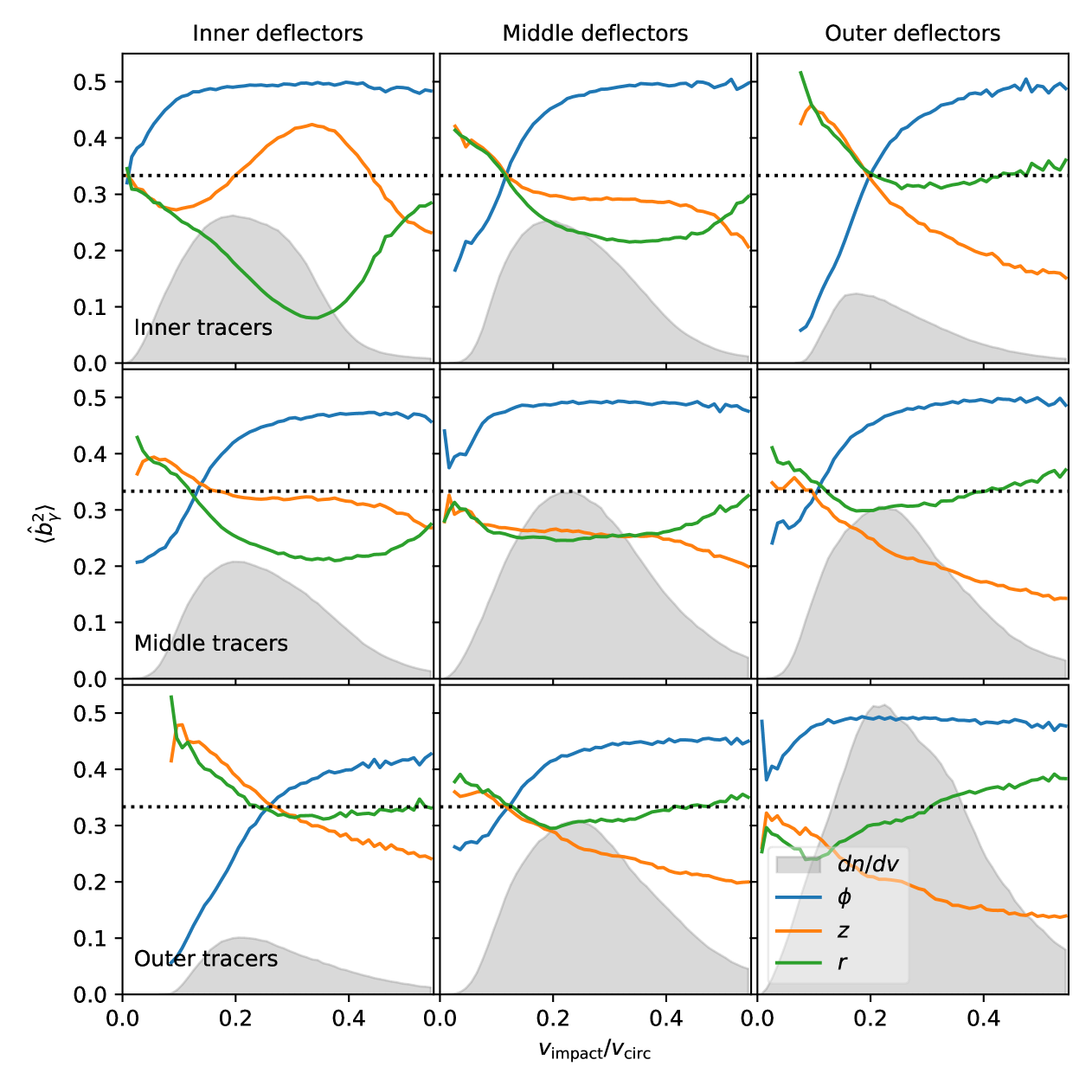
For each pair of tracer-deflector regions (e.g. Inner-Inner), we combine the list of events with the counts of candidate tracers and deflectors to calculate the event rates per eligible pair; and the mean geometry of the encounter, as a function of , all plotted in Figure 1. Here it is apparent that the component is, on average, larger than and but there is significant variation with MBA class and with . An important result is that the quantity is always well-behaved as so we do not need any special treatment to sum the integrals in Equation (15). The integrand peak is in the range
3.2.2 Asteroid properties
We crudely approximate the population as having a geometric albedo of 0.25, density of 2500 kg m and spherical shapes, which leads to the conversion
| (16) |
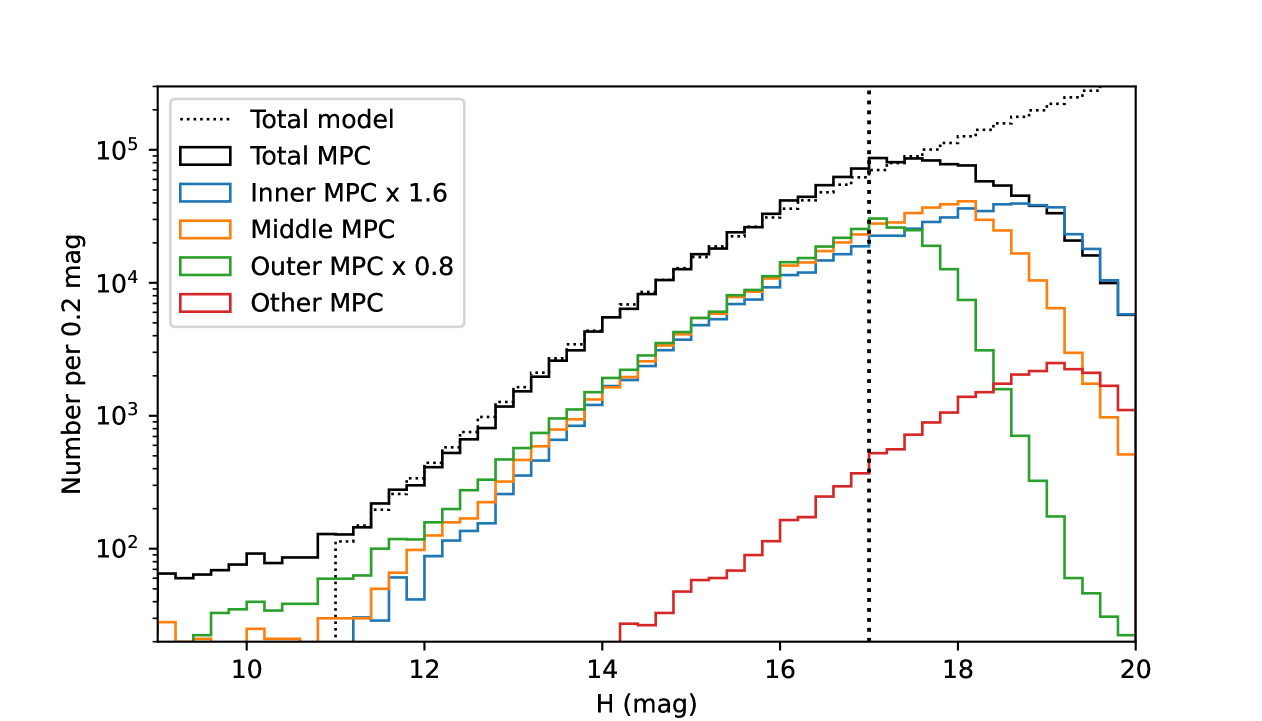
We also require the distribution of potential deflectors. Figure 2 plots our assumptions for The MPC catalog is likely close to complete in all three regions for so we will use the MPC counts directly in this regime. Note that the three regions have similar shapes of For we adopt the functional form for the cumulative MBA counts given by initial LSST predictions (LSST Science Collaboration et al., 2009):
| (17) |
normalizing this curve to the observed counts for each region.
Our integral for the uncertainty due to unmodelled MBA gravitation requires the RMS error between the true mass and the mass used (if any) in the ephemeris model. The two largest asteroids, Ceres and Vesta, have masses determined to high precision by the Dawn spacecraft (Konopliv et al., 2018, 2014). Thus despite holding half of the mass of the asteroid belt, their values333More precisely, the uncertainties in their values relative to . are and this unknown part of their contribution to other MBA’s motion is unimportant. Aside from a handful of other asteroids in well-characterized binary systems or visited by spacecraft, most other knowledge of MBA masses has and will come from mutual gravitational encounters. An individual asteroid’s mass can be estimated from its measured effect on the few MBAs on which it imparts the largest impulses. The accuracy of this determination will vary, depending upon the geometry and timing of each deflector MBA’s encounters, and the measurement errors on its tracers. These factors are independent of the mass of the deflector. We will assign a value to the RMS uncertainty in MBA mass attainable from following a few individual tracers, and calculate the Brownian-motion noise as a function of
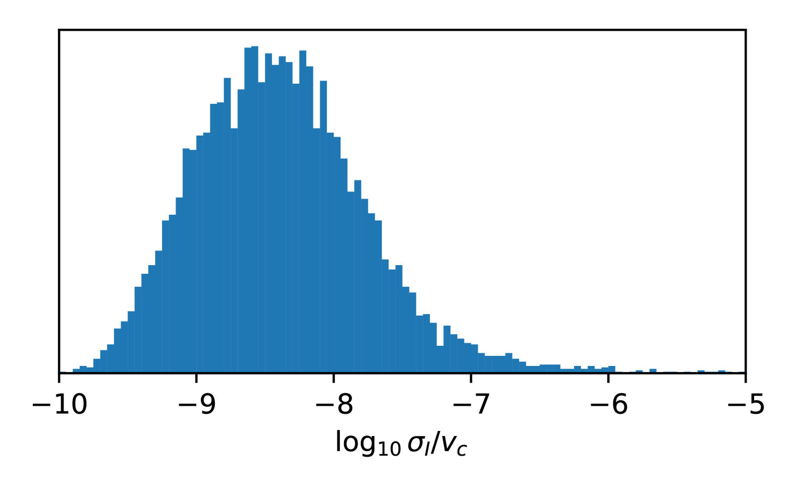
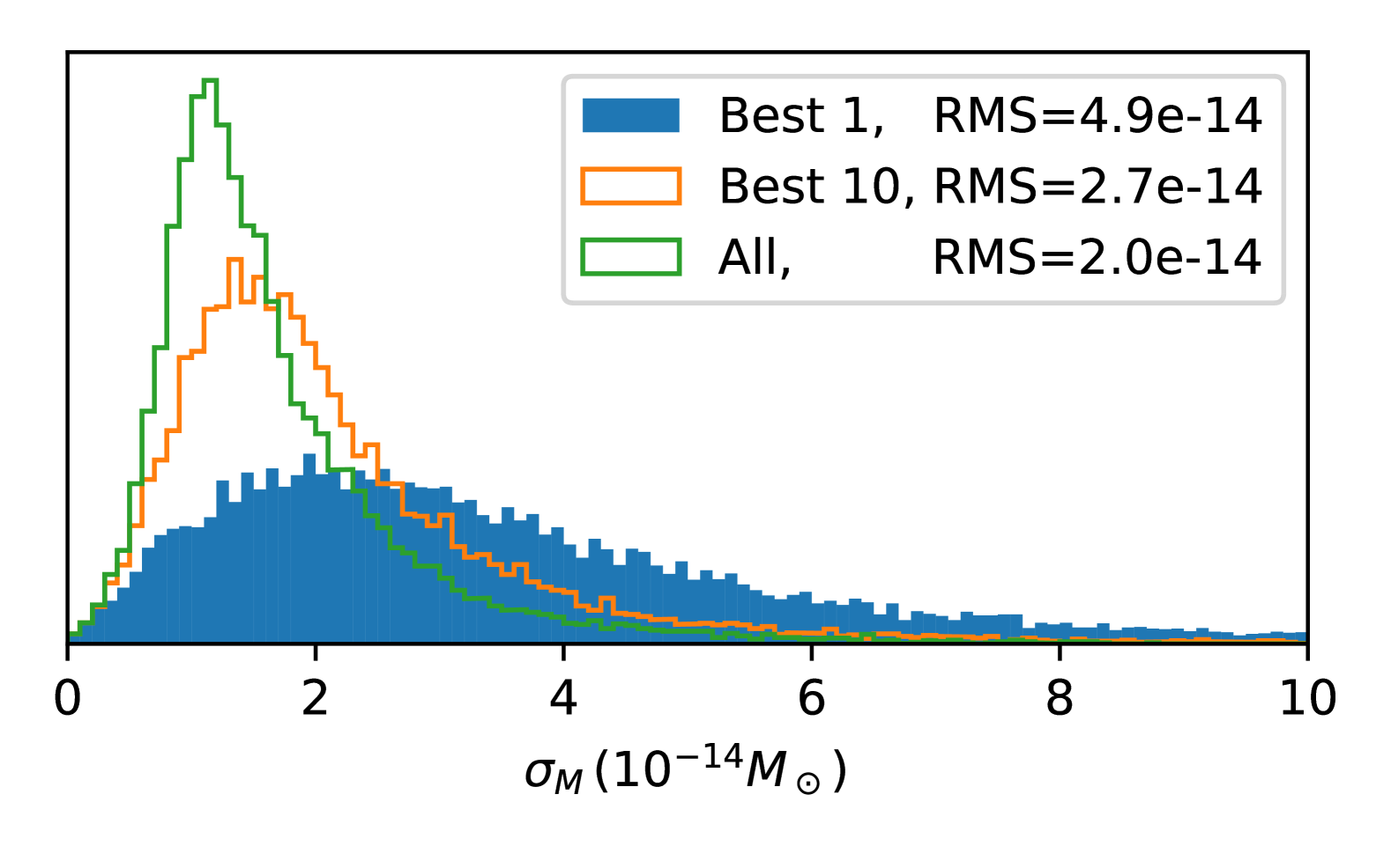
To give some context, a comprehensive investigation of MBA masses from mutual scattering events by Goffin (2014) reports typical for 30 MBAs (although the list is biased toward better-measured events). But we can expect substantial improvement in the LSST era when a millions of potential tracer asteroids attain mas-level astrometry. Bernstein et al. (2025) use a simulated LSST sequence of observations to estimate the impulse (and mass) uncertainties from analyzing LSST’s data on mutual encounters of the known asteroids. The tracer MBAs for those events are essentially an unbiased selection from the known MBAs, and the left-hand plot of Figure 3 shows the distribution of the uncertainty derived from each tracer’s LSST data after marginalizing over its initial state vector. This histogram marginalizes over the apparent magnitude and observing conditions of the tracer, the date of the encounter, and the direction of the impulse. The right-hand plot of Figure 3 forecasts the distribution of that we can expect for deflectors. This forecast is made as follows: we treat each of the 5000 tracer MBAs that we have selected from each region as deflectors, since we have a list of all of their encounters with known MBAs with AU. For each such encounter, we select at random one from the distribution for LSST data on known MBAs forecasted by Bernstein et al. (2025) (Figure 3, left), and calculate For each deflector, we then calculate (a) the individual encounter with lowest ; (b) the combined constraint from the 10 lowest encounters for that deflector; and (c) the combined constraint for all AU encounters (typically of them). The right-hand plot of Figure 3 gives the histograms of these three measures of We see that most of the available information on any given deflector’s mass comes from its 10 most-informative encounters. It should not be a computational barrier to solve for the masses of MBAs by including the deflections they impart on other MBAs in an ephemeris fit. The RMS using LSST data from the 10 most-informative tracer encounters with a given deflector is estimated as There are MBAs with mass above this forecasted RMS This is a conservative estimate in that we ignore any observational information before LSST, and we also do not consider the information increase that will come from tracking the -fold increase in number of known MBAs that LSST will enable.
3.2.3 Individually detectable impulses
Examining the distribution forecasted for LSST data on tracers by Bernstein et al. (2025), we find that for impulses occurring near the midpoint of the survey, of all cases yield some an order of magnitude lower. We conservatively assume that any encounter producing an impulse this value, can be used to directly constrain the relevant deflector and include it in the ephemeris model. When normalized by we have at 10% accuracy across the main belt.
4 Propagation to position shifts
4.1 Element shifts from impulses
The orbital shifts from an impulse can be derived from Gauss’s equations, e.g. as presented by Tremaine (2023, Section 1.9.2), but we provide here a derivation customized to our case. Five of our orbital elements will be taken from constants of the motion. The mean anomaly is not appropriate as the sixth, time-dependent element of because the derivative can diverge as Instead we introduce which we will show does have a shift during an impulse that has finite and linear response to . Between impulses, advances with the mean motion as We define a coordinate system that is uniformly rotating with the unperturbed The two smoothly rotating unit vectors and satisfy and we will use subscripts and to represent projections onto these components. In particular, the components of the ellipticity vector have the values and in the unperturbed orbit. The true anomaly radius , and azimuthal angle and the velocity components of the unperturbed orbit are, to first order in ,
| (18) |
The first element adopted for is the semimajor axis , with shift derivable from the orbital energy
| (19) | |||||
| (20) |
The initial angular momentum is altered by
| (21) | |||||
| (22) | |||||
| (23) |
We adopt the and components of the orbital angular momentum as two elements of specifying the inclination and ascending node of the perturbed orbit. These are a rotation of by the angle The conversion from the first line above to the subsequent two makes use of the decomposition derivable from the value of in Equations (18).
The eccentricity vector is altered by the impulse according to
| (24) | |||||
| (25) | |||||
| (26) |
We adopt and as two additional components of again related through a rotation by to the quantities in Equations (25) and (26).
The final element of will be The shift induced by an impulse can be obtained by enforcing the condition that the radius or the azimuthal angle must remain constant during the impulse. To find the latter, we need a formula for as a power series in Standard formulae in the literature (e.g. Tremaine, 2023) lead to:
| (27) | |||||
| (28) |
We wish to find the first-order shift in and set it to zero. But the derivatives of and with impulse can become infinite. Instead we introduce a perturbation We can now express several post-impact quantities as deviations from the unperturbed quantities:
| (29) | |||||
| (30) | |||||
| (31) | |||||
| (32) |
Forcing to be unchanged during the impulse requires
| (33) | |||||
| (34) |
We have dropped the 0 subscripts on at this point for brevity—they will refer to the values for the unperturbed orbit at the time of impulse, unless noted otherwise.
After the impulse, the mean anomaly advances at a rate of meaning that an additional term accrues by time . The total perturbation of from the nominal value becomes
| (35) |
We now have all the information we need to create the matrix. Rotating to and with we have, to ,
| (36) |
We can now do the time integral and sum over impulse directions in Equation (7), and average over to average over the orbital phase of the impulses. The diagonal elements of are
| (37) |
All of the off-diagonal terms (covariances) are either zero or and they result in observable consequences that are smaller by than the diagonal terms’ contributions.
4.2 Astrometric and ranging shifts from elements shifts
The radial coordinate of a Keplerian orbit is and an expansion of the eccentric anomaly in powers of is
| (38) |
From this we can derive the perturbations to as a function of our chosen basis for perturbations to the orbital elements. Making use of Equations (31) and (30) we obtain
| (39) |
If we square this expression, average over the orbital phase of the observation, and retain leading order in , we get the variance of the radial coordinate from the unperturbed orbit. All of the terms involving covariances between orbital elements either average to zero over an orbit, or are suppressed by relative to other terms. We are left with
| (40) | |||||
| (41) |
The second line substitutes the results from Equations (37). We retain the final term because, as this precession term that scales with becomes comparable to or larger than the other terms that scale as . The heliocentric azimuthal angle is given by Equation (32). We can similarly square the perturbation and average over orbital phase and population factors to get
| (42) | |||||
| (43) |
The heliocentric latitude (or equivalently, polar angle) has a deviation
| (44) | |||||
| (45) | |||||
| (46) |
Equations (41), (43), and (46) comprise our desired result. Several characteristics are noteworthy:
-
•
is in units of and are angles. To convert their variances into linear displacements in the directions, multiply them all by or equivalently scale the standard deviations by
-
•
The terms proportional to show typical diffusive growth and arise from random walks in the 5 constants of Keplerian motion. They represent epicyclic alterations to the original orbit that grow in amplitude as The terms dominate by the end of a full orbit, resulting from accumulating delays/advances in orbital phase as and the mean motion diffuse. Thus it is the energy-changing impulses, namely that cause the most Brownian motion.
-
•
The radial variance also becomes dominated by the term within 2 years at typical MBA values of (although nearly-circular orbits have )—this term arises from advances/delays in the radial epicycle phase. This is the only part of the Brownian motion that whose leading order in is non-zero, i.e. which we would have missed by assuming circular initial orbits.
-
•
The RMS vertical displacement grows strictly as
-
•
It will be generally true that a trend exacerbated by the empirical observation (Figure 1) that impulses favor the direction.
-
•
There are no significant covariances among the and displacements at the population-averaged level.
-
•
For Earth-based observers, the deviations in from the nominal orbit will be some calculable, time-dependent, nearly-orthonormal matrix transformation of the heliocentric deviations derived above, so the results will not be grossly different aside from bringing the three directional components closer together in amplitude.
5 Results and conclusions
We can now propagate the numerical estimates for from Section 3 through the analytical observational consequences in Section 4.2 to yield estimates of the unmodelled RMS shifts of MBAs from each region. We assume the following parameters:
-
•
The deviations are accumulated over a time yr.
-
•
The population has which is the value for the cataloged MBAs of the Inner and Middle belts, and a slight overestimate for the Outer belt.
-
•
The impulse size , at which we deem it possible to isolate the effect of a single deflector on a tracer and hence usefully include that deflector’s mass in the ephemeris model, is taken to be In practice this will depend on the geometry of the impulse and on the quality of the tracer’s observations. But we find that changing by a factor of 10 alters the noise from unmodeled impulses by
-
•
We will vary the RMS uncertainty on the mass of modelled asteroids, such that the number of MBAs with varies from 100 to 10,000. The number of MBAs included in the ephemeris model would be
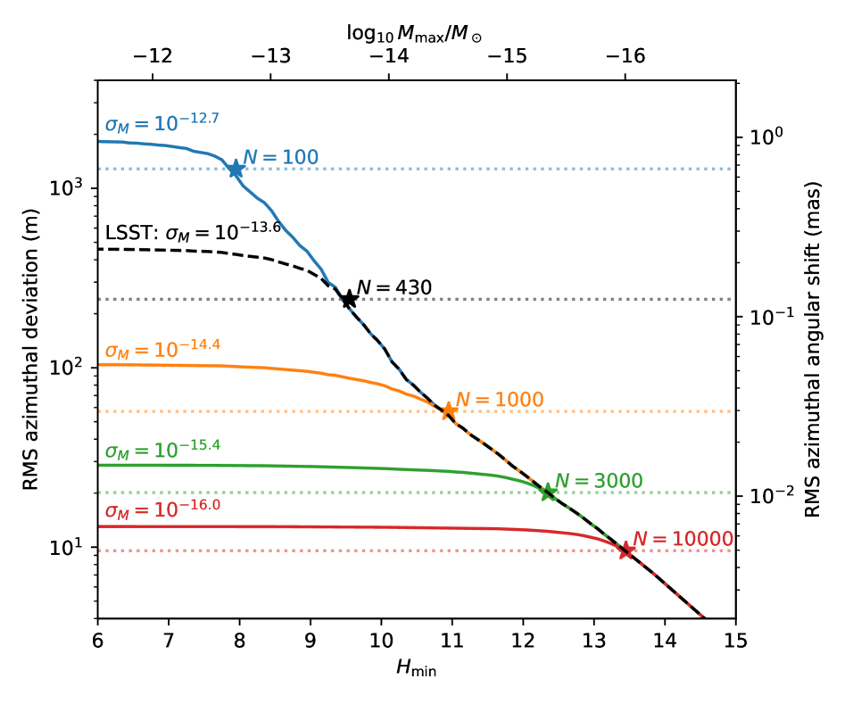
Figure 4 plots the resulting noise level of the calculation for the Middle regions of MBAs, showing both the linear RMS displacements on the left axis and the angular displacements on the right axis. Each point on the curve is the attributable to deflector MBAs that are smaller (fainter) than the value on the lower axis, or the mass on the top axis. Thus the left-most point on each curve marks the total noise integrated over the full population of deflectors. Different color lines show the results for the values of and as marked astride each line. Notable features of these result are:
-
•
The linear displacements are nearly identical for Inner, Middle, and Outer regions of the asteroid belt. The angular displacements vary slightly, inversely to their distance from the Sun. Figure 4 plots only the Middle MBAs’ deviations, although the count of modelled MBAs is the sum for all three regions.
-
•
We plot the azimuthal noise. The radial noise results have nearly identical scaling with and , but lower RMS. Likewise the vertical Brownian motion has the same shape but lower than the azimuthal RMS.
-
•
For longer time periods , the azimuthal and radial noise will scale as the vertical noise as
-
•
The largest contributions to the unmodelled Brownian motion are made by deflectors with mass and at the “shoulder” of each curve, which will also correspond to the MBAs with masses . Above this mass, the noise per deflector is constant but the deflectors become scarce at larger Below this mass, is rising to fainter/smaller bodies, but the factor that determines the Brownian motion is dropping.
We take as representative of the present state of the art the case where the most massive MBAs (aside from Ceres and Vesta) have masses determined to by mutual encounters. Our calculations suggest then that a 10-year ephemeris including these 100 MBAs will accrue RMS errors of km in the azimuthal position, or 1 mas in ecliptic longitude. RMS range and vertical ephemeris errors would be closer to 300 and 40 m, respectively. We find that, roughly speaking, drops with the number of modeled MBAs as
In the next decade, LSST will significantly increase the number of deflector MBAs with usefully measured masses from mutual encounters by tracking hugely more potential tracers and lowering The conservative estimate given in Section 3.2.2 is that LSST will lower to which our calculations indicate lowers the values to m or 0.25 mas.
We need to check whether our supposition that impulses would stand out above the measurement noise of a single tracer remains true once we include the noise induced by the other unmodelled impulses. Focusing on the effects of a tangential impulse of Equation (35) predicts an orbital phase shift of at time past the impulse, translating directly into a position shift of the same size as per Equation (32). Consider a survey of duration and a single impulse applied at time If and yr, then mas. This is much larger than the stochastic mas expected from unmodelled masses at the current state of knowledge. For primarily radial or vertical impulses, the astrometric signal will be smaller, but the Brownian motion noise is lower too. We conclude that our choice of is not ruined by the presence of Brownian motion noise on the tracer asteroids—impulses of this size will remain strongly detected.
6 Consequences
6.1 Implications for future inferences
An important question is: will the positional noise due to unmodelled MBA encounters degrade inferences being made with measurements of tracer MBAs? If the Brownian noise is well below other sources of measurement noise, then the answer must be “no.” The per-epoch uncertainties on solar-system object astrometry from Gaia444We take one Gaia transit as an “epoch” here. are reported to be as low as 0.3 mas for very bright sources (), rising to mas at its limit where most detections lie (Tanga et al., 2023, Figure 6). The overall RMS residual to the orbit fits are 5 mas (this is in the “along-track” direction). Thus the Brownian motion of mas we estimate for (over a 10-year period) with current asteroid-mass knowledge would be important for the single-epoch error budget of the brighter Gaia MBAs. With our forecasted LSST-era knowledge of asteroid masses ( RMS azimuthal errors mas), the situation will be improved in that only the brightest few MBAs will have per-epoch Brownian motion noise comparable to the per-epoch measurement noise.
For LSST, the measurement errors on MBA positions will have a floor of 1–2 mas per epoch set by refraction from atmospheric turbulence (Fortino et al., 2021; Gomes et al., 2023). Objects with apparent magnitude will have larger per-epoch errors due to photon noise in the images. Assuming that LSST inferences will be able to exploit LSST’s own determinations of MBA masses, we see that on a per-epoch basis, the Brownian noise will always be subdominant to measurement errors.
An ambitious proposal by Gomes & Bernstein (2025) is to track MBAs down to diameters of km by watching them occult Gaia stars. The timing of each occultation can locate the center of mass of the target MBA along its direction of motion, with most of the information available from objects yielding uncertainties of 50–100 m on this position. The Brownian noise (with LSST-level asteroid knowledge) over a 10-year baseline will in this case be comparable to the per-epoch measurement errors for most observations. Reducing the typical mass uncertainty of individual asteroids to would be needed () to reduce the Brownian noise to negligible levels for this survey.
These per-epoch comparisons are, however, misleading. The Brownian noise is highly correlated between different epochs of observation of a given asteroid, while the measurement errors are generally uncorrelated, and therefore the impact on inferences is not described solely by comparison of RMS values of each. The covariance structure of Brownian noise can work either to the benefit or the detriment of the inference. In an unfavorable case, the eigenvectors of the Brownian covariance matrix with the largest uncertainties look similar to the signal of interest in the inference, i.e. the derivative of the MBA’s position with respect to a parameter. If there is a single dominant eigenvector of the Brownian noise which looks just like our signal, then the per-epoch Brownian noise does not average down at all as we obtain observations, but the measurement noise drops as In a favorable case, all of the strong eigenvectors of the Brownian noise covariance are orthogonal to the signals of interest, and the Brownian noise causes no degradation of the inference, i.e. its spatiotemporal structure cannot mimic that of the signal we seek.
Consider first the worst-case scenario, where the Brownian noise does not average down at all across observations, but measurement errors drop by a factor Gaia Collaboration et al. (2023) report typically epochs per asteroid in 66 months, suggesting epochs per asteroid in the full 11-year observing period. At Gaia’s faint end, this means that Brownian noise with present asteroid knowledge would have comparable impact to the measurement errors, and dominate inferences at the bright end. LSST will obtain several hundred epochs per asteroid. With an effective factor 10–20 reduction in the total measurement noise, and assuming mas Brownian noise, the latter would become important for the brighter tracer MBAs in LSST data, but inferences with the millions of fainter objects discovered by LSST would still be limited by photon noise. The occultation program proposed by Gomes & Bernstein (2025) would obtain measurements per decade for most MBAs and hence see less degradation of Brownian relative to measurement noise.
At the other extreme are cases where the dominant modes of Brownian noise are orthogonal to the effects of parameters of interest. If, for example, one is searching for the tidal force of a Planet X, this will be manifested primarily as a collective apsidal precession and a quadrupolar deviation of the orbit from its ellipse that does not evolve with time. These are quite distinct from the random walk in that is the dominant effect of Brownian motion, and therefore Brownian noise will cause less degradation to the Planet X inference than the per-epoch would suggest. Another example would be a gravitational perturbation whose signature is primarily a nodal precession, which is a signal manifesting primarily as out-of-plane motions—we have seen that Brownian motion out of the orbital plane is smaller than the component and grows at instead of so the per-epoch of Brownian noise will grossly overestimate its effect on the inference.
The algorithms used to make inferences based on range or astrometric data will need to be changed when Brownian motion becomes a significant source of error, to accomodate the fact that positional errors on a given tracer are highly correlated between epochs. The full covariance matrix of the tracer’s observations will be needed rather than typical practice of considering measurements as independent. A small modification to our matrices would be needed to calculate the covariance of the Brownian noise between observations at different times and The Brownian motion should be fairly uncorrelated between different MBAs, because the varying encounter geometries randomize the influence of any particular deflector’s mass error on the trajectories of the tracers it influences.
A further difficulty in propagating unmodelled deflections into inferences is that the probability distribution of the position shifts will be non-Gaussian, because the RMS is dominated by the contributions of relatively few encounters with the largest unmodelled asteroids. The central limit theorem will not be applicable over decade timescales.
A better approach, however, would probably be to increase the number of MBAs considered as active bodies in the ephemeris fitting, leaving their masses as free parameters whether or not we expect them to be constrained to by the data. Although the extreme case of having active bodies’ masses as free parameters in the ephemeris fit would be a substantial computational challenge, having – should be manageable. The MBA-to-MBA perturbations can be adequately calculated using Newtonian dynamics instead of a fully relativistic treatment. In this approach, all of the covariances between different observations of the same tracer, and between tracers, will be captured in the analysis for deflections due to these deflectors. If we choose to be large enough that the Brownian noise from the unmodelled MBAs is negligible to the error budget, then we need not explicitly propagate the Brownian noise.
Figure 4 shows us what would be required: the noise due to unmodelled deflectors is given by the point where each curve for a given departs from the upper-right envelope of the curves. Increasing the number of MBAs in the ephemeris from decreases the RMS displacement in 10 yrs due to the unmodelled MBAs from m, with the radial and vertical RMS being substantially lower. These correspond to 0.7, 0.03, and 0.005 mas, respectively. Incorporating MBAs into the ephemeris model would render noise from the rest of the asteroids unimportant for nearly all uses of Gaia or LSST MBA data for inference. For occultation-based positions, one would probably want to have the most massive MBAs as active bodies with masses as free parameters in the ephemeris model in order to render encounters from unmodelled bodies as unimportant.
6.2 Comparison to radiation forces
As we consider smaller MBAs as test particles, radiation pressure becomes larger relative to gravitational forces. It is interesting to compare the effects of radiation pressure to those of Brownian motion to see when the former are a bigger source of noise than the latter, or contrarily to see whether Brownian motion interferes with attempts to measure radiation forces on MBAs. At first order, radiation pressure from the Sun and the reaction from reflected sunlight cause a constant radial force on the MBA. The ratio of this force to the gravitational force for an asteroid of radius geometric albedo , and density is where
| (47) |
where the last expression adopts our standard values The primary observational consequence of this constant radial force is a time-independent, -dependent shift of the radial position a body should have at a given period. This does not resemble any expected effect of Brownian motion, and also very difficult to measure since radar ranging to MBAs is infeasible. More important for observations is the Yarkovsky effect, in which anisotropic re-emission of the absorbed radiation leads to a net force that is a fraction of the incident radiation pressure. The Yarkovsky effect has been detected for several NEAs but no individual MBAs, with values (Yarkovsky effect and data are review by Vokrouhlický et al., 2015). This is also consistent with detections of the Yarkovsky effect by examining the dependence on of members of asteroid families in the Main Belt (e.g. Nesvorný & Bottke, 2004).
The Yarkovsky effect has in common with Brownian noise that it has the strongest observable effects via changes to and the mean-motion rates, and that these changes can be of varying sign and amplitude for a given asteroid. In the case of the Yarkovsky effect, this variability arises because of the random orientations of spin axes, and differences in spin rates, shapes, and surface properties.
Taking a case where the Yarkovsky force is in the prograde azimuthal direction, and using our system of units with and this leads to a continuous power which in turn implies The mean motion rate is hence and the accumulated shift in mean anomaly over time amounts to In this case, a rough comparison of the accumulated from the Yarkovsky effect to the of noise from unmodelled Brownian motion, after a time interval , is
| (48) |
if we assume from the current knowledge of asteroid masses. There is thus a break point near , or m diameter: for MBAs larger than this, the ephemeris uncertainties from the Yarkovsky effect will be smaller than those from mutual gravitational encounters on decade timescales. This includes all MBAs detected by Gaia and nearly all detectable by LSST. Below this size, the Yarkovsky displacement grows larger in a decade and has a better chance of being detectable in the presence of Brownian motion. Distinguishing the steady quadratic growth of the Yarkovsky from the random-walk growth of Brownian motion to the same final size requires observational S/N and time resolution significantly better than is needed for detecting either one individually.
When Yarkovsky forces on MBAs are estimated using the -dependent dispersion of for asteroid families, the effective “observation” time period is typically several Myr. Over these long time scales, Equation (48) shows that the temporally coherent Yarkovsky effect can dominate over Brownian motion for bodies up to 10’s or 100’s of km in diameter, which is why the technique is successful.
6.3 Summary
In conclusion, the Brownian motion from unmodelled or mis-modelled mutual impulses between MBAs causes RMS azimuthal displacements of km (or 1 mas in angular position) over 10 years, with current knowledge of the masses of large asteroids. This is large enough to become a significant part of the error budget for many inferences from Gaia MBA astrometry. The knowledge on large-MBA masses likely to be gained from LSST tracking of MBAs should reduce this by a factor of at which point the Brownian noise will be comparable to Gaia or LSST measurement uncertainties only for the brighter targets of each survey. In all cases, the Brownian motion is smaller in the radial direction and in the vertical direction. The RMS azimuthal and radial displacements grow with time as , and the vertical RMS as
Making inferences from MBA astrometry becomes more complicated when Brownian motion is a significant contributor to the error budget, but a good path forward is to do all model fitting by including the largest MBAs as active bodies in the ephemeris model and leaving their masses as free parameters. This will constrain the masses of these bodies to the full extent that the data allow, and will properly propagate any remaining uncertainty in those masses into the other inferences that one is trying to make. The noise contributed by the remaining millions of unmodelled MBAs would be just m RMS in the azimuthal direction (about 30 as), and a few as or less in the other axes, small enough to ignore entirely for the accuracy of imaging astrometry for the foreseeable future. Occultation-based astrometry is much more accurate (but has fewer possible measurements per tracer), and would be significantly impacted by Brownian motion until MBAs have mass estimates at modest level, although the precise impact will depend on whether the signals one is seeking are parallel or orthogonal to the kind of variations caused by Brownian motion. For objects m in diameter, uncertainties from mutual encounters are larger than uncertainties from the Yarkovsky effect over decade timescales, at present levels of knowledge of asteroid masses.
References
- Baer & Chesley (2017) Baer, J., & Chesley, S. R. 2017, AJ, 154, 76, doi: 10.3847/1538-3881/aa7de8
- Bernstein et al. (2025) Bernstein, G., Najafi, N., & Gomes, D. 2025, \psj, in preparation
- Fienga et al. (2020a) Fienga, A., Avdellidou, C., & Hanuš, J. 2020a, MNRAS, 492, 589, doi: 10.1093/mnras/stz3407
- Fienga et al. (2020b) Fienga, A., Di Ruscio, A., Bernus, L., et al. 2020b, A&A, 640, A6, doi: 10.1051/0004-6361/202037919
- Fortino et al. (2021) Fortino, W. F., Bernstein, G. M., Bernardinelli, P. H., et al. 2021, AJ, 162, 106, doi: 10.3847/1538-3881/ac0722
- Gaia Collaboration et al. (2023) Gaia Collaboration, David, P., Mignard, F., et al. 2023, A&A, 680, A37, doi: 10.1051/0004-6361/202347270
- Goffin (2014) Goffin, E. 2014, A&A, 565, A56, doi: 10.1051/0004-6361/201322766
- Gomes & Bernstein (2025) Gomes, D. C. H., & Bernstein, G. M. 2025, \psj, 6, 19, doi: 10.3847/PSJ/ad9f5b
- Gomes et al. (2023) Gomes, D. C. H., Murray, Z., Gomes, R. C. H., Holman, M. J., & Bernstein, G. M. 2023, \psj, 4, 66, doi: 10.3847/PSJ/acc7a2
- Holman & Payne (2016) Holman, M. J., & Payne, M. J. 2016, AJ, 152, 94, doi: 10.3847/0004-6256/152/4/94
- Konopliv et al. (2014) Konopliv, A. S., Asmar, S. W., Park, R. S., et al. 2014, Icarus, 240, 103, doi: 10.1016/j.icarus.2013.09.005
- Konopliv et al. (2018) Konopliv, A. S., Park, R. S., Vaughan, A. T., et al. 2018, Icarus, 299, 411, doi: 10.1016/j.icarus.2017.08.005
- LSST Science Collaboration et al. (2009) LSST Science Collaboration, Abell, P. A., Allison, J., et al. 2009, arXiv e-prints, arXiv:0912.0201, doi: 10.48550/arXiv.0912.0201
- Mariani et al. (2023) Mariani, V., Fienga, A., Minazzoli, O., Gastineau, M., & Laskar, J. 2023, Phys. Rev. D, 108, 024047, doi: 10.1103/PhysRevD.108.024047
- Nesvorný & Bottke (2004) Nesvorný, D., & Bottke, W. F. 2004, Icarus, 170, 324, doi: https://doi.org/10.1016/j.icarus.2004.04.012
- Park et al. (2021) Park, R. S., Folkner, W. M., Williams, J. G., & Boggs, D. H. 2021, AJ, 161, 105, doi: 10.3847/1538-3881/abd414
- Pitjeva & Pitjev (2018) Pitjeva, E. V., & Pitjev, N. P. 2018, Astronomy Letters, 44, 554, doi: 10.1134/S1063773718090050
- Tanga et al. (2023) Tanga, P., Pauwels, T., Mignard, F., et al. 2023, A&A, 674, A12, doi: 10.1051/0004-6361/202243796
- Thoss & Burkert (2024) Thoss, V., & Burkert, A. 2024, arXiv e-prints, arXiv:2409.04518, doi: 10.48550/arXiv.2409.04518
- Tremaine (2023) Tremaine, S. 2023, Dynamics of Planetary Systems (Princeton University Press)
- Vokrouhlický et al. (2015) Vokrouhlický, D., Bottke, W. F., Chesley, S. R., Scheeres, D. J., & Statler, T. S. 2015, in Asteroids IV, ed. P. Michel, F. E. DeMeo, & W. F. Bottke (University of Arizona Press), 509–531, doi: 10.2458/azu_uapress_9780816532131-ch027