The Simons Observatory: Quantifying the impact of beam chromaticity on large-scale -mode science
Abstract
The Simons Observatory (SO) Small Aperture Telescopes (SATs) will observe the Cosmic Microwave Background (CMB) temperature and polarization at six frequency bands. Within these bands, the angular response of the telescope (beam) is convolved with the instrument’s spectral response (commonly called bandpass) and the signal from the sky, which leads to the band-averaged telescope beam response, which is sampled and digitized. The spectral properties of the band-averaged beam depend on the natural variation of the beam within the band, referred to as beam chromaticity. In this paper, we quantify the impact of the interplay of beam chromaticity and intrinsic frequency scaling from the various components that dominate the polarized sky emission on the tensor-to-scalar ratio, , and foreground parameters. We do so by employing a parametric power-spectrum-based foreground component separation algorithm, namely BBPower, to which we provide beam-convolved time domain simulations performed with the beamconv software while assuming an idealized version of the SO SAT optics. We find a small, , bias on , due to beam chromaticity, which seems to mostly impact the dust spatial parameters, causing a maximum bias on the dust -mode spectra amplitude, , when employing Gaussian foreground simulations. However, we find all parameter biases to be smaller than at all times, independently of the foreground model. This includes the case where we introduce additional uncertainty on the bandpass shape, which accounts for approximately half of the total allowed gain uncertainty, as estimated in previous work for the SO SATs.
1 Introduction
Measurements of the Cosmic Microwave Background (CMB) polarization are at the forefront of cosmological research, as they offer insights into the origins and evolution of the Universe. Of particular interest is the measurement of the CMB -mode polarization anisotropies (the parity-odd component of the CMB polarization) as a probe of the very early Universe and a strong test of the inflationary paradigm. Cosmic inflation is the current leading theory explaining the initial density perturbations, and the Universe’s large-scale homogeneity and flatness. It postulates a brief period of exponential expansion of an initially small patch of the infant Universe into its current observable size. The primordial quantum fluctuations, stretched by this expansion to cosmological scales, leave traces in the spacetime metric in the form of both scalar and tensor perturbations. The latter, also referred to as gravitational waves, are the only primordial source of CMB -mode fluctuations, with scalar modes only sourcing the parity-even -modes. By measuring both components of the CMB polarization, we can quantify the amplitude of primordial gravitational waves generated by inflation, and thus probe the high-energy physical processes that caused it. This amplitude is commonly parametrized in terms of the ratio between the amplitudes of the power spectrum of primordial tensor and scalar perturbations, [11, 26, 52].
Cosmological -modes are significantly smaller than the -mode perturbations. In addition, on the large, degree-sized scales where the sensitivity to the primordial signal is highest, the polarized sky is dominated by emission from Galactic foregrounds [27, 37, 47]. Thus, the accuracy with which we can measure is tightly linked to our ability to properly characterize these foregrounds and, crucially, the impact of all instrumental effects on the measured signal. To cleanly separate the cosmological signal from any other contaminants, the CMB community has developed a large variety of component separation methods (e.g. [4, 21, 13, 43, 47]) that rely mostly on the frequency-dependent Spectral Energy Distributions (SEDs) of the foregrounds to distinguish them from the CMB’s nearly perfect blackbody spectrum [18]. However, the performance of any of these methodologies depends strongly on the impact of instrumental systematics on the data and on our ability to mitigate or model them. For -mode experiments, great care must be taken when modeling the systematic effects related to the telescope’s optics. In particular, improper modeling of the telescope’s spatial response, namely the telescope’s Point-Spread-Function (PSF), commonly referred to as the telescope’s beam, can cause leakage of the stronger CMB temperature signal into the fainter polarization data, as well as mixing between the - and -modes [15].
An important aspect of beam modeling is linked to the beam’s intrinsic frequency dependence. As CMB telescopes typically observe radiation over wide frequency bands instead of monochromatic frequency channels, it is natural to expect some variation in the beam properties within each band. The impact of this beam ‘chromaticity’ is further complicated when the beam is convolved with frequency-dependent sky components with differing spectral signatures. It is worth noting that, due to these differing spectral signatures, the chromaticity effects will vary slightly for each component. Further complications arise when additional beam non-idealities are present. Representative examples include pronounced beam power at large angles away from the beam center (sidelobes), non-negligible polarization in the direction orthogonal to the detector’s polarization direction (cross-polarization), as well as beam asymmetry [45, 15, 30]. For sufficiently complex beams and foregrounds, if these effects are not taken into account in the analysis, they may give rise to significant biases in the inferred model parameters. Therefore, these effects must be quantified to determine the most reliable estimate of the instrumental beam to employ in the component separation analysis [32, 40].
Although these beam-related biases are typically sub-percent at the power spectrum level, they can still threaten the high-accuracy requirements of current and next-generation CMB missions [28] such as the Simons Observatory (SO) [2]. By observing the polarized microwave sky from the Chilean Atacama desert in six frequency bands centered between and , the SO Small Aperture Telescopes (SATs) [20] aim to constrain with a statistical uncertainty of or better. Given the broad observing bands of the SATs, with relative fractional bandwidths, it is crucial to model the impact of the anticipated beam frequency dependence on the large-scale -mode spectra. We do so in this paper, starting from time-domain simulations convolved with chromatic beams that we then analyse using a power-spectrum-based component separation pipeline. An estimation of the corresponding impact on scientific objectives relevant to the SO Large Aperture Telescope (LAT) [54, 53] like the effective number of relativistic species, , and amplitude of unresolved radio sources in temperature, , is presented in [23]. That work assumes a LAT-like experiment and Gaussian beams with perturbed FWHM values, which are applied to the simulated data at the power spectrum level.
The paper is structured as follows: Section 2 introduces the individual components that form the telescope’s band-averaged beam and describes the specifics of the beam simulations. Section 3 elaborates on the sky model assumptions and methods employed for the beam-convolved simulations, the power spectra estimation, and the foreground component separation algorithm. The results are presented in Section 4, including the impact of beam systematics of non-frequency-dependent beams, the inclusion of the beam chromaticity effect as a function of foreground complexity, and any further biases caused by the integration of bandpass uncertainty in the model. Finally, Section 5 summarises the paper and outlines potential directions for future studies.
2 Spectral dependence of beam response
The SO SATs observe the microwave sky at frequency bands of approximately width around the center frequencies. Assuming a detector on the focal plane characterized by an instrumental bandpass, , and beam response, , at frequency , we can derive the band-averaged beam of the detector as follows:
| (2.1) |
This formula assumes integration only over frequency and incorporates the SED of the observed sky component denoted by expressed in antenna temperature units. The beam is described in terms of both the polar angle, , and the azimuthal angle, , allowing for beam asymmetry by introducing a dependency on the position angle in the time-ordered data. Note that, while the source emission will not be spatially constant, we avoid adding its orientation dependence in this equation, which describes the synthesis of the band-averaged beam. The spatial dependence of is taken into account properly in the sky simulations.
To generate the SAT Physical Optics (PO) beam simulations, we assume the same optical configuration (three-lens refracting telescope) as for the work described in [12] and employ the TICRA TOOLS111TICRA, Landemærket 29, Copenhagen, Denmark (https://www.ticra.com). software. Specifically, we produce monochromatic far-field beam maps for four frequency bands roughly centered at , , , and , respectively. Each of these Mid- and Ultra-High-Frequency (MF and UHF) bands has relative width around its center frequency, and to each band correspond five monochromatic beam maps evenly spread across the full frequency range of the band. Note that we have two MF and two UHF bands as the SATs employ dichroic detectors. For the nominal case, we assume a detector located at the center of the focal plane. We then integrate across the full band in each case, employing the original or perturbed versions of the simulated bandpasses presented in [1]. The beams of the Low-Frequency (LF) bands, which are roughly centered at and , are approximated using Gaussian curves of FWHM equal to and , respectively. This approach is sufficient at this stage since the SO SATs will dedicate only a small part of their full scanning time to LF observations. Furthermore, we ensure in Appendix A that the partial treatment of only the MF and UHF bands as chromatic PO beams does not impact the analysis results. We do, however, plan to generate PO simulations for the LF beams and integrate them into the pipeline in future work.
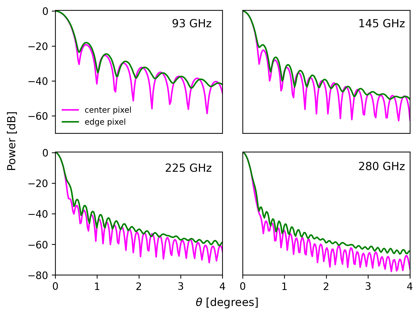
The resulting beam models include both asymmetric and cross-polar components, as well as faint far sidelobes. Note, however, that these beam models are still the product of ideal simulations of the SO SAT optics222More realistic optics simulations could, for example, include non-ideal baffling elements or reflective Half-Wave-Plates (HWPs), like the effects discussed in [14]. . In reality, we may expect more pronounced beam non-idealities arising from the optical setup. The logarithmic profiles of the monochromatic co-polar beams for the MF and UHF bands are shown in Figure 1. From the figure, we observe the profiles ‘contracting’ with increasing frequency within each band, as expected for a diffraction limited beam. The asymptotic yellow curve in the bottom right panel, representing the highest frequency of the band, highlights the challenge posed by the numerical precision of the PO simulations. Since the computational costs of the simulations scale as frequency squared, the accuracy with which the simulation converges on a solution is also frequency-dependent. At the limits of the machine’s precision, very low beam power will, therefore, be approximated to be at the convergence threshold, creating a constant-looking sidelobe at large angles. Note that, while these will be the beam models used throughout the paper, we also estimate the best-fit forecast parameters in the case where we have underestimated the chromaticity of the beam by a smaller and larger value of and change, respectively, inside the band (see Appendix D).
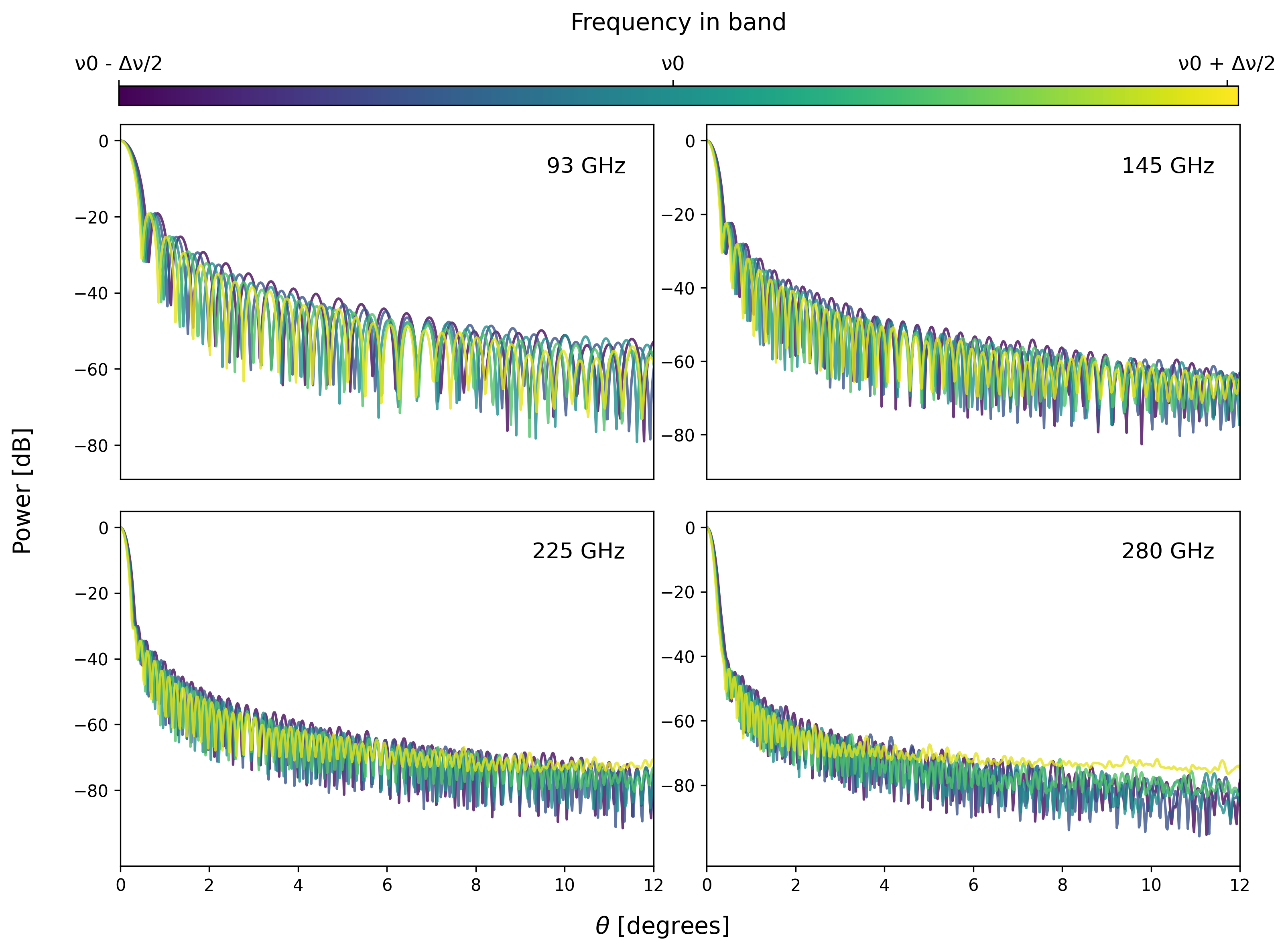
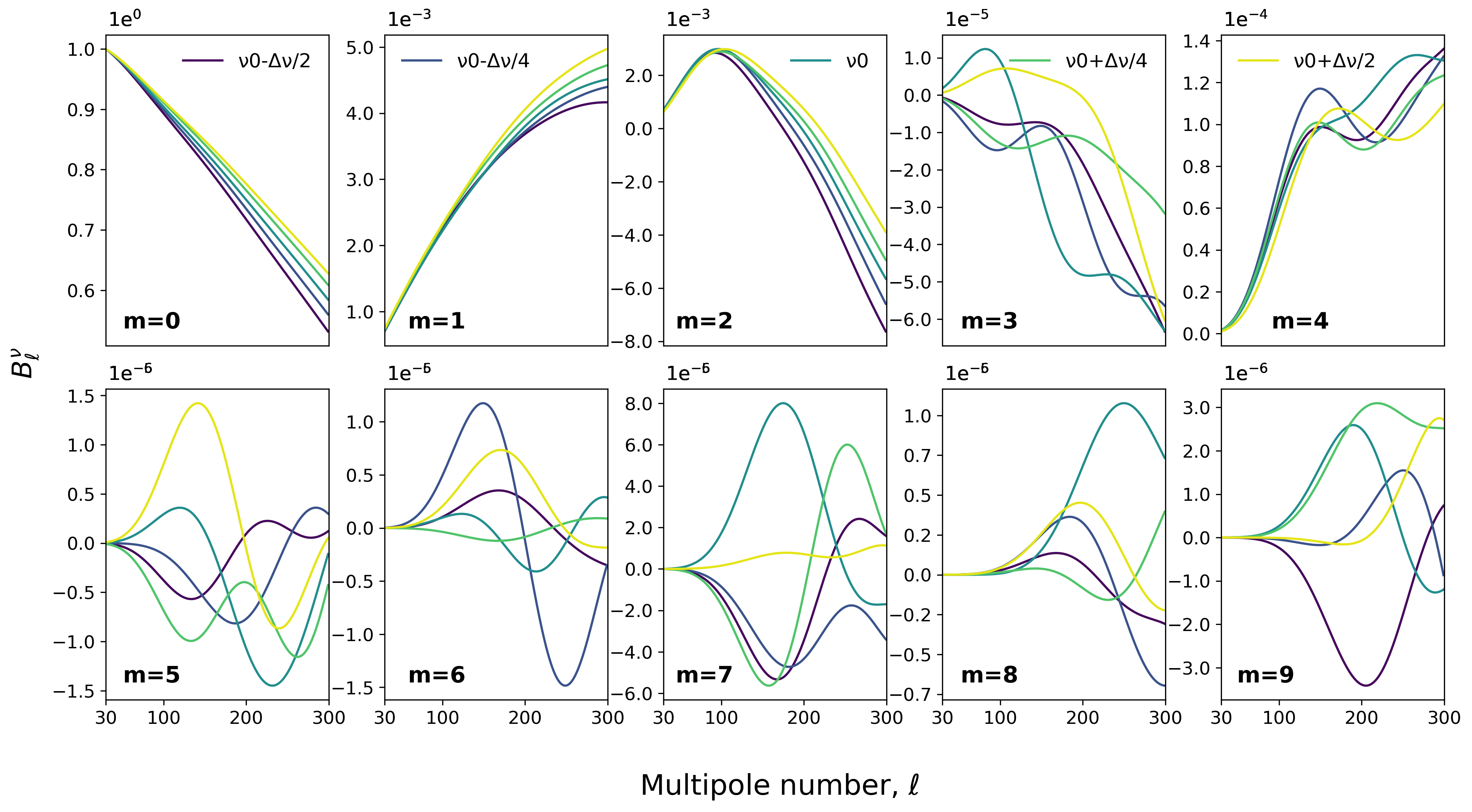
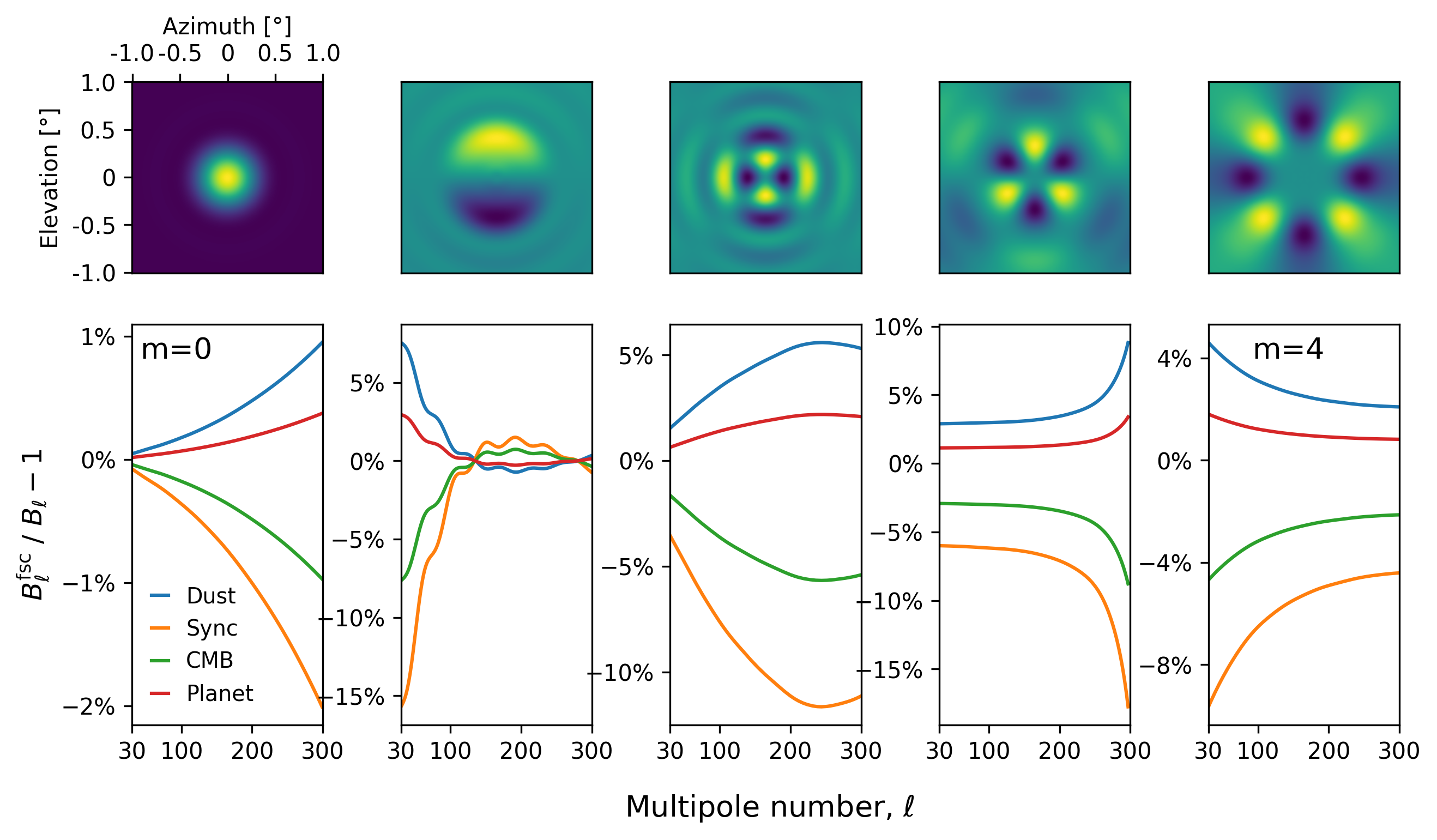
Figure 2 illustrates the frequency-dependent beam variation in the harmonic domain utilizing the monochromatic beams of the band (MF1), shown in the top left panel of the previous figure, as a representative example. The plots show the harmonic transforms for the first ten azimuthal beam modes, , spanning multipoles in the range . This is the range we will be employing throughout this paper for consistency with [51]. For the symmetric part of the beam (m=0), increasing the frequency widens the beam transfer function. The impact on the rest of the modes, nevertheless, is not as straightforward to capture. To decide on the number of beam modes we employ in the analysis, we refer to the expected calibration accuracy for the MF and UHF bands of the SO SATs. The beam of the band that is shown in this example is expected to be calibrated within a accuracy for multipoles spanning [12]. In principle, this means we can ignore any modes that are smaller than three orders of magnitude with respect to the main beam. However, we choose to allow for a margin of error and include all azimuthal modes that contribute at least relative to the m=0 beam. These correspond to the first five azimuthal modes for the MF1 beam. We ensure this approach is consistent across all four frequency bands.
The combined frequency scaling of the beam and the sky components results in a net frequency-dependent scaling of the band-averaged beams, as shown in Equation 2.1. That depends on the observation and is generally different from simply averaging the beam over the bandpass. To illustrate the interplay between the intrinsic beam chromaticity and the frequency dependence of different sky components, we compute the band-averaged beam transfer function by assuming a source SED that corresponds either to pure Galactic dust, synchrotron radiation, CMB or planets (commonly used as beam calibrators). The bottom panel of Figure 3 presents the percentage ratio of the frequency-scaled transfer function, , relative to the nominal band-averaged transfer function, , which assumes a constant SED. Both cases are produced employing the first five azimuthal beam modes, as displayed in Figure 2. These modes are also shown in map space for the constant SED beam in the top panel of the same figure. In each case, the sky component’s SED is the one also used in the employed component separation pipeline (see Section 3.1). Note that the TICRA TOOLS simulations employed in this work only include the beam intrinsic frequency dependence, corresponding to the case where the calibrated beam which will be used in the analysis has already been corrected for the SED of the calibration source (see Section 4.5 of [46]). From the figure, we observe the symmetric beam component varying as much at the highest multipoles, whereas the frequency-scaled asymmetric modes show deviations from the corresponding azimuthal mode’s constant-SED beam of up to (the non-frequency scaled m=1-4 modes remain, however, three to five orders of magnitude smaller than the corresponding m=0 beam).
3 Methods
To assess the impact that beam chromaticity has on the cosmological analysis, we produce beam-convolved simulations in the time domain, bin them into maps, and estimate their pseudo-, -mode power spectra, which we then utilize to derive the best-fit values for the tensor-to-scalar ratio, , and foreground parameters. We do so for both chromatic and achromatic beams and quote the bias between the two cases on the forecast parameters in terms of each parameter’s expected uncertainty in the achromatic beams scenario.
3.1 Sky model
The assumed sky model is comprised of CMB, Galactic dust, and synchrotron emission. To simulate CMB sky maps, we draw Gaussian random realizations of the CMB power spectra assuming the Planck best-fit CDM parameters [38] and no tensor fluctuations (). In our fiducial analysis, we also simulate dust and synchrotron as (uncorrelated) Gaussian realizations of their corresponding and spectra as measured by the Planck and WMAP experiments [39, 47, 27] (see Section 3.3 of [51]). We will, however, repeat part of our analysis using realistic, non-Gaussian foreground realizations (see Section 4.2.2), as this is particularly important for beams carrying pronounced far sidelobes that may pick up the signal from strongly emitting Galactic sources.
The sky SEDs are given by a blackbody law for the CMB, a modified blackbody law (at fixed temperature K) for thermal dust, and a power law for synchrotron. The free parameters in the sky model, which will be later fitted for, are the tensor-to-scalar ratio, , the amplitude of lensing -modes, , the spectral indices for dust and synchrotron, and , the amplitude and spectral tilt of the dust and synchrotron -mode power spectra, denoted as , , and , and the dust-synchrotron correlation parameter, . The CMB power spectrum employed for the Gaussian realizations is computed as:
| (3.1) |
The templates employed for and correspond to lensing-only -modes and tensor-only -modes of amplitude = 1, respectively, and are precomputed by CAMB [29]. The amplitudes and scaling factors for Galactic dust and synchrotron are linked through a power law that describes the input spectra for these two components:
| (3.2) |
with = 80. Since this paper focuses on the beam chromaticity-induced bias on CMB -mode analysis, we restrict ourselves to a straightforward sky model and do not include more complex features such as spatial variability of the foreground spectral properties. Biases of the latter type are discussed in [5, 6, 51].
3.2 Beam-convolved simulations
Random realizations of the different sky components are generated from a known model of their power spectra, as described above333The code used for the sky simulations is available at https://github.com/susannaaz/BBSims. We generate maps of NSIDE=256 at five single frequencies uniformly sampled across a 25 bandwidth around the center frequency of each MF and UHF band. These single-frequency sky models are provided as input to beamconv444https://github.com/AdriJD/beamconv [15] along with the corresponding simulated SAT beams for the same frequencies. The software is equipped with a ground-based scanning function, which we employ to approximate the scan strategy of the SATs by simulating a telescope located in the Atacama Desert in Chile, performing observations informed by the nominal SAT scan strategy (see Section 2.3 of [48]). We use a wide Field-Of-View (FOV) of matching the corresponding size of the actual telescope, populate the focal plane with two hundred detector pairs that are spread uniformly across a square grid, and simulate year-long observations sampling the sky at . While there is dedicated software for SO time-domain simulations, namely the Time-Ordered Astrophysics Scalable Tools (TOAST555https://github.com/hpc4cmb/toast) and sotodlib666https://github.com/simonsobs/sotodlib packages, we choose to employ beamconv for this study due to the latter’s reduced computational cost and the fact that no noise or atmospheric simulations are needed. At this stage, we choose not to simulate the SAT Half-Wave-Plate (HWP) since our main aim is to assess the impact of beam chromaticity independently of the systematics arising from the beam and HWP coupling. For HWPs comprised of three birefringent layers, as is the case for one of the SO SATs, the coupling between the beam chromaticity and the frequency-dependent angle offset associated with this type of HWP could introduce additional challenges [16].
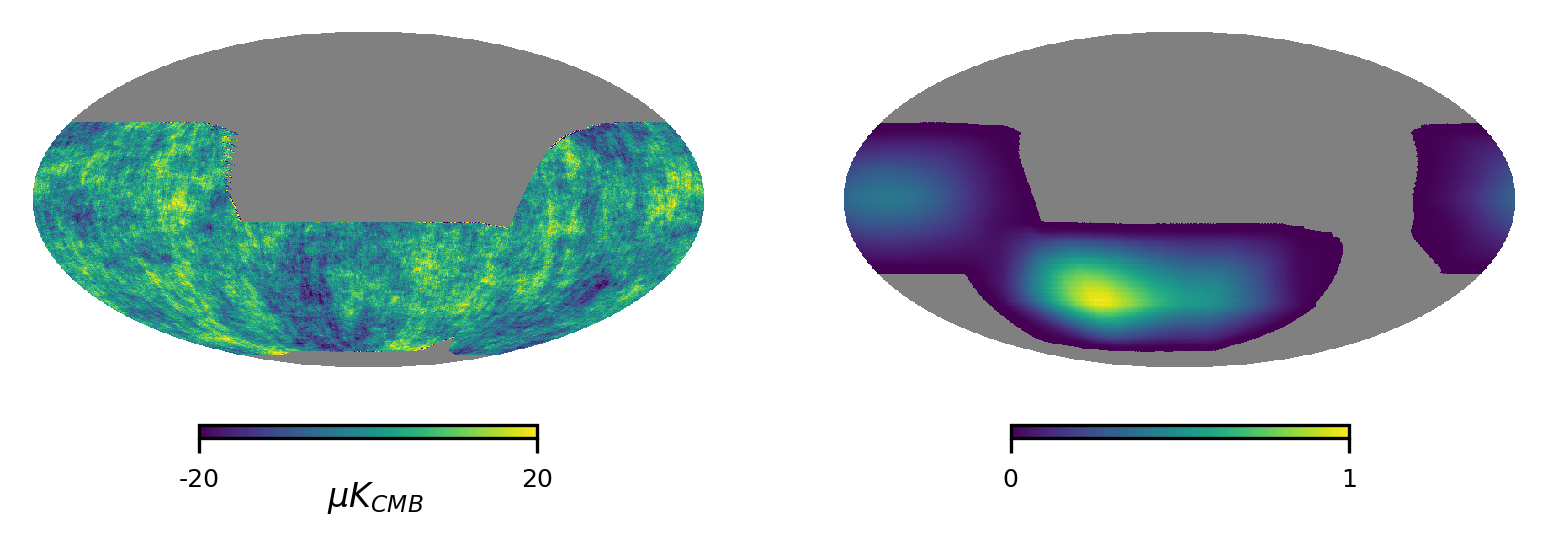
The sky templates are produced only for the Stokes Q and U components while a zero temperature map is provided to beamconv. This is done to exclude any contributions from -to- leakage in the analysis and for consistency with the work of [51]. After the input polarization maps are beam-convolved in the time domain, they are transformed back into maps using a ‘naive’ mapmaker that simply bins the time-ordered data into pixels given the pointing. An example of a monochromatic map at produced this way is shown in Equatorial coordinates in the left panel of Figure 4. In total, for each sky realization, we obtain six maps corresponding to the six SO frequency bands; four of them constructed using PO chromatic beams (MF, UHF) and two using achromatic Gaussian beams (LF). The band-averaged map of each of the MF and UHF bands is the result of applying the (nominal or perturbed) bandpass to the corresponding (five) monochromatic maps. The right panel of the same figure shows the apodized mask that is applied to the beam-convolved maps and is created from the detector hits of the simulated scan strategy. This mask is fairly similar to the SO SAT mask defined in [48] and used in [51]. However, the latter was an early estimate that did not employ the scan strategy, and, thus, we choose to use the mask that is informed from the hits map produced in beamconv.
Masking the sky results in mode-mixing, which we need to estimate and correct for when reconstructing the angular spectra. Assuming no noise contributions to the data, the pseudo- power spectra, , can be connected with true spectra, , as follows [22, 3]:
| (3.3) |
The matrix is the mode-mixing kernel, capturing the statistical coupling between different harmonic-space modes caused by the sky mask while represents the beam transfer function. We make use of the pseudo- power spectrum estimator as implemented in NaMaster777https://github.com/LSSTDESC/NaMaster [3]. In particular, we make use of -mode purification [42], which projects out the contribution from true (i.e. full-sky) -modes that leak into the observed -modes due to mode mixing caused by the sky mask. -mode purification reduces the power spectrum variance on the large scales by order 50% or more, depending on the noise level, and is therefore crucial for achieving SO’s projected precision of [48]. Beam convolution, on the other hand, reduces the observed signal power spectrum on the small scales, effectively up-weighting the instrumental noise contribution, and increasing the uncertainty on the parameters sensitive to >150, such as . The beam deconvolution in NaMaster is performed by including only the symmetric component of the beam in the mode-mixing matrix, . Hence, we can expect a slight bias when estimating the power spectra of maps convolved with asymmetric beams using this method (see Section 4.1), or when using the incorrect beam transfer function due to the chromaticity effects discussed above.
Finally, some degree of bias is to be expected when employing time-domain simulations instead of an analytic approach using the (true) component spectra. Simple binning mapmakers like the one beamconv uses are limited by the degree of cross-linking they can get in each pixel. They are also subject to sub-pixel errors [34]. The bias on the resulting spectra between the two approaches is shown in Appendix A and is further quantified in terms of the corresponding impact on the tensor-to-scalar ratio and foreground parameters.
3.3 -mode analysis pipeline
For the foreground component separation, we use a power-spectrum-based algorithm as implemented in BBPower888https://github.com/simonsobs/BBPower, which is introduced in [1, 5, 6] and in [51], where it is referred to as ‘Pipeline A’. The code consists of two main stages, one to compute power spectra from maps, and another one to perform power-spectrum-based component separation and parameter inference. We use both stages when running on the binned time-domain simulations, and only the second stage when cross-checking with (true) analytical power spectra.
Stage 1 uses NaMaster to compute -mode-purified cross-frequency power spectra from a set of input maps of the partial sky. The purification algorithm requires a smoothed input sky mask, which we obtain by apodizing the hits map corresponding to our simulated SAT scanning strategy described above. As in [51], we choose an analysis range of , and adopt multipole bins of width 10 to increase the numerical stability of the mode coupling matrix. One aspect to note is the fact that if the asymmetric modes of the beam are significant, then the standard purification would not be optimal since it would not clean up the ambiguous -modes caused by the asymmetric beam. This could lead to additional variance in the estimator and potentially bias the -mode power spectra.
Stage 2 carries out component separation and parameter inference at the same time. Specifically, given the full set of -mode auto- and cross-power spectra between the six different SO SAT frequencies, BBPower builds a forward model for these measurements incorporating the contribution from both CMB and foregrounds. Using a likelihood for the measured spectra, it then derives the posterior distribution of all foreground and CMB parameters at the same time. The methodology is similar to that used by BICEP-Keck [7]. Here we use Gaussian likelihood to describe the distribution of the cross-frequency bandpower amplitudes999Although the power spectrum of a Gaussian field generally follows a Wishart distribution, the binned bandpowers contain a sum over sufficiently many independent modes so that the central limit theorem guarantees approximate Gaussianity. As verified in [51], choosing a Gaussian likelihood in the present setup (, , SAT sky patch) is sufficiently accurate.. The forward model that constitutes the mean of this distribution is built by combining the contributions of all sky components (: CMB, : synchrotron, : dust):
| (3.4) |
The first term above contains the autocorrelations of all sky components, while the second term describes the correlation between dust and synchrotron emission, quantified by the parameter . The auto-spectra of the different components are described by the same models outlined in Section 3.1. Note that we expect the combination of potential model mismatch with beam chromaticity to be worrisome only in cases of fairly complex foreground models like the ones including frequency de-correlation. The model mismatch in such cases can be compensated using the method of moments extension to the model [5] and dust marginalization techniques [3]. The small mismatch that can be seen between the Gaussian and non-Gaussian cases we study in this work can be absorbed by employing wide priors for the parameters of the (fairly generic) fitting model. The full set of nine parameters entering the likelihood is:
| (3.5) |
The theoretical prediction is evaluated at all integer multipoles and then convolved with the bandpower window functions provided by NaMaster. The bandpower covariance is the same as the one described in [51], estimated from 500 simulations of coadded Gaussian CMB, foregrounds, and SAT-like noise in the ‘baseline-optimistic’ scenario [48]. The latter assumes isotropic noise, incorporating contributions from both white and 1/f noise components, with observations covering of the sky over a total duration of five years for the MF and UHF bands and one year for the LF bands, respectively. The posterior distribution is sampled using the emcee Markov Chain Monte-Carlo code [19], assuming prior distributions given in Table 1 101010The (unphysical) negative values for are employed to track volume effects from biases in other parameters (as explained in [51]). Volume effects in the posteriors can bias the cosmological parameters due to noisy (foreground) data and will be investigated in future work..
| Parameter | Prior type | Bounds |
|---|---|---|
| TH | [0.0, 2.0] | |
| TH | [-0.1, 0.1] | |
| G | 1.54 0.11 | |
| TH | [-1.0, 1.0] | |
| TH | [-1.,0.] | |
| TH | [0,) | |
| G | -3 0.3 | |
| TH | [-2.,0.] | |
| TH | [0,) |
4 Results
The results presented in this section are produced by employing simulations that are a mix of only CMB, Galactic dust, and synchrotron in all cases. To avoid mixing potential beam-related bias with the noise bias, we deliberately exclude any noise contributions from the simulations. The covariance estimate used by the component separation pipeline is the one described in [51] and includes the noise variance, cosmic variance, and foreground uncertainty estimates. After assessing the significance of non-ideal beam properties for this analysis, we demonstrate the impact of beam chromaticity on the forecast parameters for both Gaussian and non-Gaussian foreground models, considering cases with and without bandpass uncertainty.
4.1 Bias from beam systematics
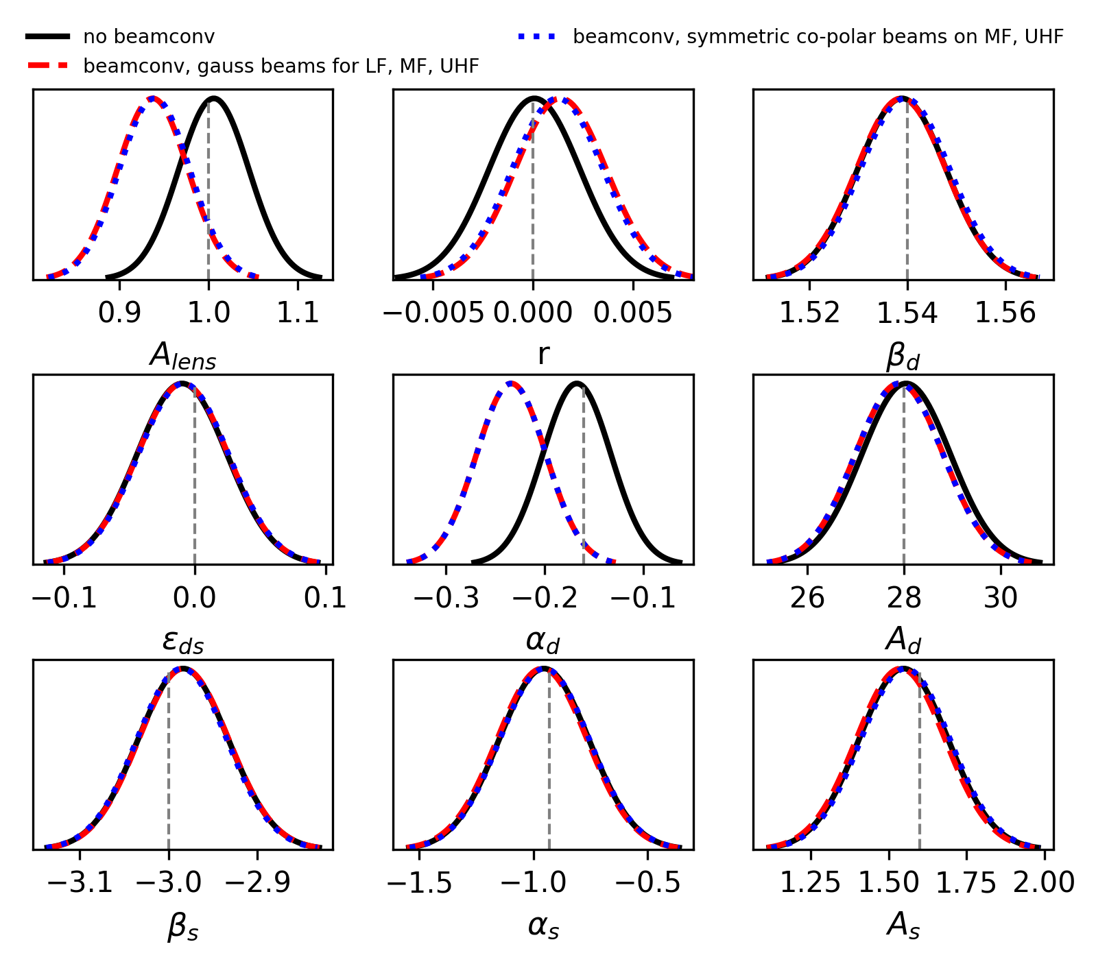
In order to quantify the impact of different beam non-idealities in the inferred model parameters, we employ sky realizations that include CMB and Gaussian foregrounds and carry out four different types of beamconv simulations only for the center frequencies of the MF, UHF bands using (non-chromatic) beams of scaling complexity. The LF beams are also approximated as Gaussian beams in this case. The different types of simulations include (i) symmetric co-polar beams, (ii) symmetric co- and cross-polar beams, (iii) asymmetric co- and cross-polar beams, and (iv) asymmetric co- and cross-polar beams, including (low-amplitude) far sidelobes. For cases (i)-(iii), we truncate the beams to a maximum angle of while for case (iv), we use the full angular range of the beam simulations, extending to . The beam transfer function employed for the deconvolution is the one of case (i) in all cases. We chose to use a small number of sky realizations for computational efficiency, and we find them to be enough to capture any significant parameter biases caused by beam non-idealities. This is also aided by the fact that the simulations used are noiseless, although they still include cosmic variance. The estimated best-fit parameters for the four beam cases, assuming only the center frequencies of the bands and averaged over ten different sky realizations 111111We observed that the forecast parameters tend to converge rapidly, typically within the range of five to ten simulations. It also appears that the accuracy of the forecast parameters does not show substantial improvement beyond this threshold., are depicted in Figure 5 through their one-dimensional posteriors. These are obtained by averaging the posterior distributions of each parameter across all sky realizations.
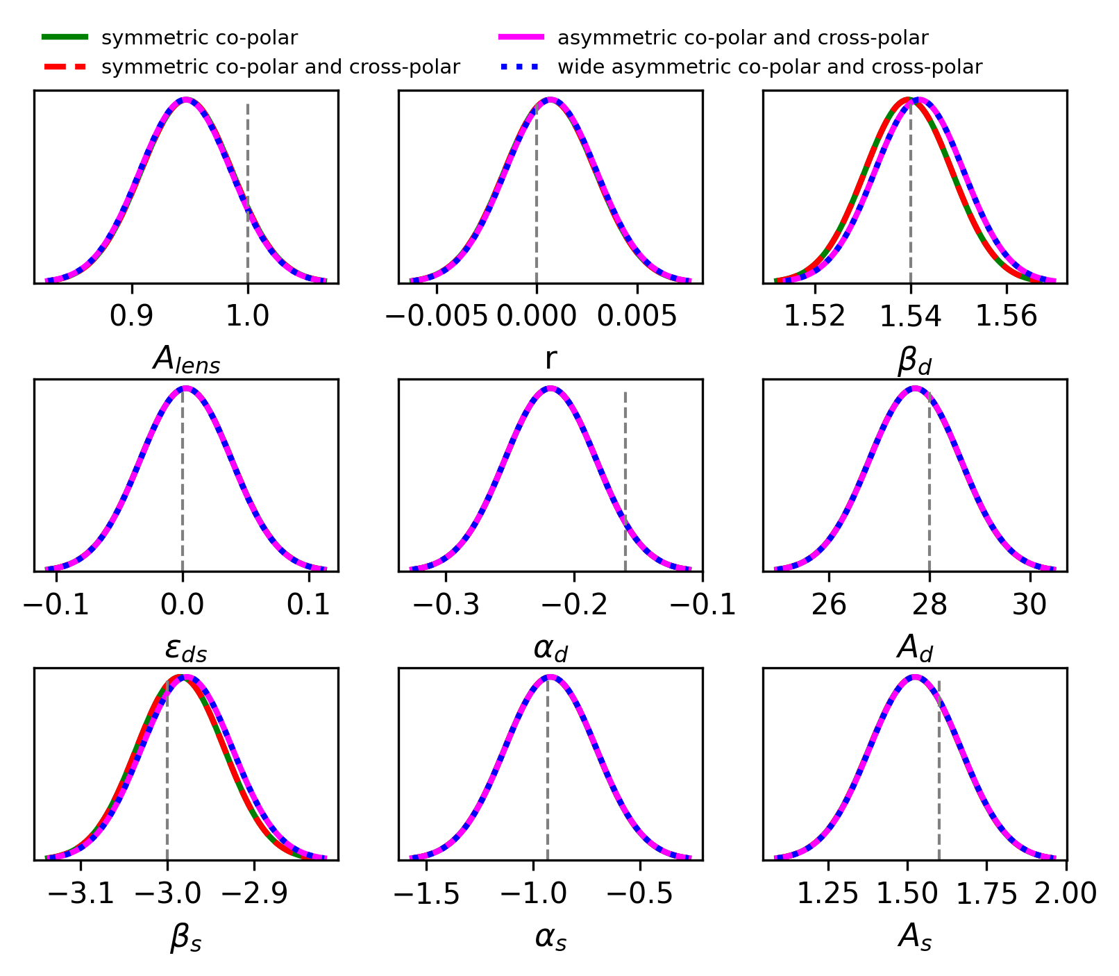
The inclusion of the simulated symmetric cross-polar beam (red) does not appear to change the estimated values of the forecast parameters as compared to the symmetric co-polar beam simulations (green). This is likely due to the small relative amplitude of the cross-polar component (see Appendix B). However, the results for the asymmetric beam simulations do display small, but still visible, deviations, both for the narrow (magenta) and wide beams (blue). In particular, we can see two distinct sets of distributions forming for the spectral indices of dust and synchrotron ( and ), depending on whether or not the employed beams include asymmetric components. This is because an asymmetric beam induces a frequency-dependent asymmetry in the maps, and the most direct way for the likelihood to interpret this is through a shift in the spectral parameters of the foreground components. The bias induced by beam asymmetry is approximately for both and , where represents the average uncertainty across all sky realizations in the symmetric co-polar beam scenario. This type of bias significantly outweighs any additional bias from the beam’s far sidelobes, which are much fainter than the main beam (by six to eight orders of magnitude compared to the amplitude at the beam center). Note, however, that these statements solely refer to the beam systematics derived from our ideal optics simulations and may not accurately reflect the challenges present in real-world conditions. The in-band beam chromaticity, though, is a consequence of the diffraction-limited optics of the SATs and is not expected to change, even if, for example, we observe larger amplitudes in the far sidelobes when modeling the beams from planet observations. The reason for assessing the beam systematics present in the simulations was, thus, only to showcase they are not strong enough to mask the chromaticity effect we want to capture. Another relevant remark to make here is that beam asymmetry can introduce -to- leakage, which the HWP is expected to prevent. The contribution of the HWP in mitigating this type of leakage is thoroughly discussed in [44]. The HWP is also expected to reduce beam asymmetry, further mitigating the effect seen in the spectral indices of the galactic foregrounds. Consequently, the previous results could be further verified by also simulating temperature scans and including the SATs HWP in the assumed optical setup.
Any residual bias between the symmetric co-polar beam simulations and the input parameter values is primarily due to the integration of beamconv into the pipeline and, to a lesser extent, to deviations of these beams from perfect Gaussian distributions. The former is further discussed in Appendix A where, similarly to Figure 4.1, we see small biases in all parameters with a visible difference in the posteriors of and when employing beamconv in the simulations. While we expect a small difference in all parameters due to the use of a mask motivated by the scan strategy (as opposed to the simple estimate for which these parameters were recovered in [51]), and are particularly affected by the loss of power at small scales which occurs due to the sparse distribution of detectors on the focal plane (we use two hundred detector pairs as opposed to the few thousand detectors present on the actual SAT focal plane). This choice was made with respect to the computational efficiency we wanted to achieve 121212A full set of chromatic beam simulations for a given foreground model can be performed within a week.. However, any bias between the analytic and beamconv cases is included both in the chromatic and non-chromatic beam simulations and does not, thus, impact the results.
4.2 Chromatic beams
4.2.1 Gaussian foregrounds
We now repeat our analysis, applying our component separation pipeline to ten sets of six beamconv maps (one per observing band) that were simulated employing the approximated SAT scanning strategy described in the previous section. The simulations are performed for the center frequencies of the LF bands assuming Gaussian beams and for five single frequencies within each of the MF and UHF bands, using monochromatic PO beams that include asymmetry, cross-polarization, and far sidelobes. The best-fit tensor-to-scalar ratio and foreground parameters are then derived from band-averaged maps that were created by applying the reference bandpasses from [1] to the MF, UHF monochromatic maps and compared against the case where only the center-frequency maps were used for all bands. Note that the beam used to deconvolve the power spectra in the current and following sections is the harmonic transform of the symmetric center-frequency or band-averaged beam (for the achromatic and chromatic cases, respectively) and includes both the co- and cross-polar response.
The average values of the best-fit parameters from these ten simulation sets are shown in Table 2 and are denoted as ‘Chromatic’ or ‘C’. The corresponding parameters, where frequency bands are represented solely by their center frequencies, are also provided for reference. These are labeled as ‘Achromatic’ or ‘A’, and are presented alongside the input values assumed in the simulated sky configuration.
| Parameter | Input | Achromatic (A) | Chromatic (C) | |
|---|---|---|---|---|
| 1 | 0.94 0.04 | 0.93 0.04 | 0.18 | |
| 0 | 1.320 2.282 | 1.369 2.305 | 0.02 | |
| 1.54 | 1.540 0.009 | 1.538 0.008 | 0.17 | |
| 0 | -3.375 34.65 | -0.35 32.33 | 0.09 | |
| -0.16 | -0.229 0.035 | -0.239 0.031 | 0.27 | |
| 28 | 27.8 0.9 | 27.1 0.7 | 0.77 | |
| -3.0 | -2.992 0.051 | -2.979 0.051 | 0.24 | |
| -0.93 | -0.918 0.197 | -0.920 0.194 | 0.01 | |
| 1.6 | 1.57 0.14 | 1.56 0.14 | 0.06 |
The last column presents the bias between the chromatic and achromatic beams scenario in terms of the anticipated uncertainty for each parameter in the achromatic case.
Upon examining the table, we conclude that the most noticeable effects of beam chromaticity apply to the Galactic dust parameters, with the amplitude of the dust spectra inheriting a bias when chromatic beams are employed in the simulations. On the contrary, the tensor-to-scalar ratio, , appears to be largely insensitive to the beam’s frequency dependence. This is due to the fact that the constraining power on is at degree scales (around ), thus the beam systematics that are more pronounced at the higher multipoles, like chromaticity (see Figure 3), have very little effect. This is different from the impact on other parameters like the lensing amplitude, which does depend on what happens at . Furthermore, the small values associated with the synchrotron spatial parameters should be interpreted with caution throughout the analysis results in this and the following sections. This is because they are primarily informed by the LF bands, where the simulations did not account for the beam chromaticity effect. All parameters, however, show deviations smaller than .
Finally, it is worth noting that the beam chromaticity bias on is not expected to increase even if a non-zero input value of is chosen in the fiducial model. We would, however, find a larger value for due to the added cosmic variance. Moreover, the most significant biases are observed on the dust spatial parameters ( and ), which are known to be largely uncorrelated with , unlike the spectral index , which remains largely unaffected. Nevertheless, a follow-up study could ensure that this is the case. The interplay between the input (0 versus 0.01) and foreground anisotropy was studied using the same pipeline in [51], see Table 5.
4.2.2 Non-Gaussian foregrounds
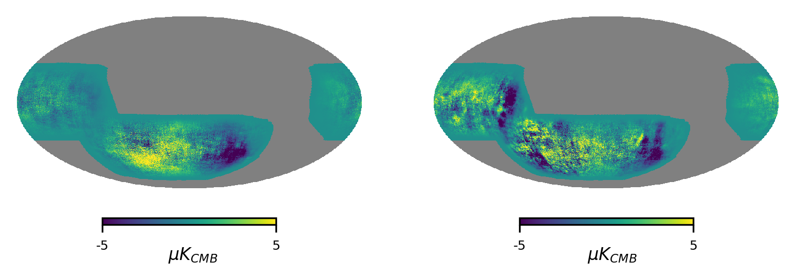
We proceed by assuming non-Gaussian foregrounds and repeating the steps described in the previous section. In this case, we use the PySM module to produce template maps of dust emission and synchrotron radiation that describe, once again, a modified black-body distribution and power-law, respectively. These foreground models correspond to models ‘d0’ and ‘s0’ of the PySM package and are commonly used as representative non-Gaussian test models [24, 51]. The spectral indices of synchrotron and dust are constant across the sky, but the template maps now include the large-scale anisotropies caused by the Milky Way. Much of the emission from the Galactic plane is removed from the simulated maps by applying the mask described in Section 3.2. Figure 6 shows the Stokes Q maps generated for the lowest (left) and the highest (right) band center frequencies, namely and , using the ‘d0s0’ model. An important remark at this stage is that these non-Gaussian simulations display a larger dynamic range that could be picked up by the beam sidelobes. The best-fit parameters obtained by combining chromatic beams with non-Gaussian foreground models are presented in the same manner as for the Gaussian case. Table 3 summarizes the average values from ten simulation sets, utilizing both achromatic and chromatic beams. It also presents the biases between these two cases, estimated as a function of the expected uncertainty per parameter.
| Parameter | Input | Achromatic (A) | Chromatic (C) | |
|---|---|---|---|---|
| 1 | 0.94 0.04 | 0.93 0.04 | 0.14 | |
| 0 | 0.916 2.273 | 0.930 2.283 | 0.01 | |
| 1.54 | 1.539 0.007 | 1.539 0.007 | 0.01 | |
| - | 35.7 49.5 | 46.7 46.2 | 0.22 | |
| - | -0.318 0.036 | -0.335 0.033 | 0.47 | |
| - | 34.1 1.1 | 33.4 1.0 | 0.53 | |
| -3.0 | -3.05 0.09 | -3.05 0.09 | 0.15 | |
| - | -1.579 0.303 | -1.597 0.293 | 0.06 | |
| - | 0.63 0.14 | 0.63 0.14 | 0.02 |
Note that we do not provide input values for , , , , and , in the first column as, in this case, the spatial properties of the dust and synchrotron maps are determined by the data on which PySM is based, rather than any input power spectrum. The best-fit values for the power law parameters of the dust and synchrotron power spectra instead depend on the particular sky region targeted. Furthermore, one should consider that, even though the Galactic plane is largely removed when masking the data, strong emission from that region may still leak into the unmasked footprint via the beam sidelobes (especially at the mask edges), potentially impacting the fitted parameters. However, it is important to note that the values of and used to generate the Gaussian simulations discussed earlier are determined as the best-fit values derived from a large sample of ‘d0s0’ maps (without any additional beam convolution) and the analysis mask described in [51]. The choice to use a Gaussian likelihood also for non-Gaussian foregrounds is motivated by the same work, where the authors tested that the chi-squared statistic computed for non-Gaussian foregrounds and using the simulation-based covariance discussed ealier agreed with the expectations for Gaussian data (see Appendix A of the same publication).
As in the case of Gaussian foregrounds, the largest bias corresponds to the dust spatial parameters, and , at approximately for both parameters. It is, however, interesting to notice the increased bias of the dust-synchrotron correlation parameter, ( as compared to in the Gaussian foreground scenario). Independently of the foreground model assumed, the two components are convolved with the same beam and the fitting code can interpret the additional frequency scaling introduced by the beam as additional correlation between the foregrounds. This result is more obvious for the non-Gaussian simulations (that already include some level of dust-synchrotron correlation) described in Table 3 but note that it also applies to the quoted values of Table 2. The beam frequency scaling increases also the correlation between the Gaussian dust and synchrotron components. In fact, the slight anti-correlation observed in the achromatic beam scenario is nearly eliminated when beam chromaticity is included in the simulations. Overall, the chromaticity bias on all forecast parameters remains approximately below the level, even when we assume non-Gaussian foreground models.
4.3 Impact of bandpass uncertainty
Bandpass uncertainty can arise due to variations in the fabrication process of the filters or from inherent systematics present in their measurements conducted using a Fourier transform spectrometer [41, 36]. It can also be the result of frequency-dependent reflections between elements in the optical system. Spectrally averaging over a finite bandwidth can help in mitigation. However, care needs to be employed to ensure the methodology used to characterize the receiver elements does not differ from the as-used configuration at a level that influences the calibration data acquired [8]. Time-varying atmospheric fluctuations further contribute to bandpass variations by inducing alterations in the frequency-dependent atmospheric transmission. These factors collectively influence fluctuations in both the effective gain and central frequency of the bandpass as explained in [50]. A detailed analysis of the bandpass calibration requirements for the SO SATs is provided in [1], where the allowed bandpass variation is quantified in terms of effective frequency and gain. According to this work, both of these parameters must be known to percent level or better. Note that these constraints are designed with respect to avoid biases of the order of on the tensor-to-scalar ratio, , measuring which is the primary scientific goal for the SATs.
The gain can be expressed as the integrated product of the telescope’s effective area, , the instrumental bandpass, and the instrument’s beam response:
| (4.1) |
Since the authors of [1] employ achromatic beams in the analysis, we attribute the majority of gain variations to arise from bandpass variations. As the requirement for the bandpass center uncertainty has already been studied in the same publication, we focus on the bandpass shape variations, which we parametrize in terms of an effective gain variation, , and a slope, , from the reference bandpass. In this way, we construct a set of ten perturbed bandpass curves, , for each of the MF and UHF bands as follows:
| (4.2) |
The effective gain variation, , is drawn for each frequency, , from a Gaussian distribution that is centered on one and has a standard deviation equal to times the frequency’s reference bandpass value. Furthermore, the scaling factor, , is allowed to assume ten discrete values uniformly sampled from the range of [-1, 1].
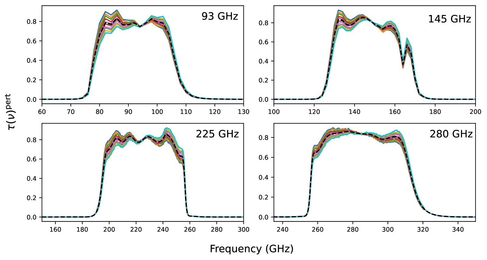
As shown in Figure 4 of [50], the amplitude of the bandpass variations allowed by our parametrization is comparable with those originating from realistic atmospheric variations and the frequency-dependent scaling from the sky components, and the range of slopes covered here is significantly larger. The ratio between each perturbed bandpass integrated over the full frequency range and the corresponding value for the reference bandpass does not exceed for the MF bands and for the UHF bands. These upper boundaries represent approximately half of the allowed percent gain uncertainty determined in [1], ensuring that the bias on does not exceed the desired limit. Figure 7 shows the newly constructed perturbed bandpasses (curves of various colors) for all bands considered in this work, plotted against the reference bandpasses (black dashed lines).
We now construct ten new versions for each of the ten sets of band-averaged beamconv maps used in the analyses discussed in Sections 4.2.1 and 4.2.2, one for each of the new perturbed bandpasses. We assume the same input sky realizations as before and quantify the combined impact of beam chromaticity and bandpass fluctuations on the forecast parameters for both the Gaussian and non-Gaussian foreground scenarios. Since we have assumed the perturbed (by an offset and slope) bandpass curves to center around the nominal bandpasses, the average bias over all different bandpasses per sky realization with respect to the results of the same realization when the nominal bandpass is used should be zero. For this reason, we choose to compute the standard deviation of the best-fit parameters across all bandpasses for a given sky realization instead. The estimated standard deviation is then averaged over all sky realizations as well and compared to the expected standard deviation per parameter in the achromatic beam, nominal bandpass scenario. For the Gaussian case, we find the interplay of frequency-dependent beams with bandpass variations to add , , , , , , , , and to the total anticipated uncertainty, , associated with the determination of , , , , , , , , and , respectively. Similar results hold also for the non-Gaussian case, with the uncertainty increasing by , , , , , , , , and for the same parameters. Once again, we observe a larger effect on the amplitude and tilt of the dust -mode power spectra ( and ), independent of our assumptions about the foreground model. In the non-Gaussian case, however, there is also a larger effect in the additional uncertainty on the tensor-to-scalar ratio, although it remains small, at the level. Once again, the negligible added uncertainty for the synchrotron parameters should be interpreted carefully, as they are predominantly informed by the LF bands, the maps of which are only convolved with achromatic beams.
5 Conclusion and Discussion
In this paper, we present the method and associated pipeline for quantifying the beam chromaticity impact on the large-scale -mode power spectra of the SO SATs, through the constraints on the tensor-to-scalar ratio, , and foreground parameters derived from them. The method entails:
-
•
Simulating five monochromatic PO beams for each of the MF and UHF frequency bands, at frequencies evenly spanning the band’s full frequency range.
-
•
Performing the time-domain convolution of simulated sky templates with these beams while assuming a SAT-like scan strategy, using beamconv.
-
•
Estimating the power spectra of these beam-convolved maps after masking and minimizing, correcting for -to- leakage, and employing -mode purification techniques with NaMaster.
-
•
Using these spectra to determine the best-fit values for the tensor-to-scalar ratio, lensing amplitude, and foreground parameters, employing BBPower.
We perform the analysis assuming both Gaussian (Section 4.2.1) and non-Gaussian foreground models (Section 4.2.2) and also study the interplay between beam chromaticity and bandpass uncertainties (Section 4.3).
The beam simulations used in this analysis are generated assuming a three-lens refracting telescope, representing the fundamental optical configuration of the SO SATs (see Section 2). We find that most non-idealities present in the achromatic beam simulations, like asymmetry or cross-polarization, are not expected to impact significantly the best-fit values and accuracy of the tensor-to-scalar ratio and foreground parameters (as shown in Section 4.1). Note, however, that these beam non-idealities will be further modeled from real planet observations, and we will then assess again their impact, though we do not expect any major effect for this analysis. The ten sky realizations provided to beamconv contain CMB, Galactic dust, and synchrotron at the same frequencies as the beam simulations and the convolution happens assuming a SAT-like scan strategy.
When considering Gaussian foregrounds, we find that beam chromaticity leads to a negligible bias on the tensor-to-scalar ratio (). In turn, most of the effect is absorbed by the parameters characterizing the spatial structure of Galactic dust, recovering a bias on the -mode power spectrum amplitude, , of (see Table 2). We find similar results when repeating the analysis on more realistic, non-Gaussian foregrounds (PySM model ‘d0s0’). The largest impact is again on the spatial dust parameters, with both and biased at the level (see Table 3). Nevertheless, the constraints on remain comparably unaffected. This is not unexpected considering that beam chromaticity impacts mostly the higher multipoles (see Figure 3) while most of the constraining power for is at large scales (). Furthermore, the dust-synchrotron correlation increases when beam chromaticity is accounted for in the simulations, and this effect is independent of the employed foreground model.
In addition to quantifying the net effect of beam chromaticity, we also consider variations in the bandpass shape and evaluate how these couple to the beam frequency dependence. We do so by applying an effective gain and slope perturbation to the fiducial SO SAT bandpasses (the impact of uncertainties in the effective frequencies was studied in [1]). Repeating our analysis for ten different realizations of the instrument bandpasses, perturbed in this manner, we find that the impact is once again largely absorbed by the foreground spatial parameters. We compute the standard deviation of the best-fit parameters for a given sky realization over all the employed (perturbed) bandpass curves and then average over all realizations. We estimate an additional uncertainty of between and for the dust amplitude and spectral tilt , depending on the foreground model. The parameter again denotes the expected parameter uncertainty in the achromatic beam, nominal bandpass scenario. The impact on all other parameters is significantly smaller.
While this analysis indicates that in-band beam chromaticity is unlikely to cause significant bias on the tensor-to-scalar ratio and foreground parameters, there are still future directions to explore within the same scope. A key example is the development of more advanced beam simulations to establish a clear link between the complexity of the beam and the resulting bias in the foreground parameters. Appendices B and C already commence this work by assessing the cases where we scale up the beam cross-polarization and ellipticity. Another important component in this context is the SAT HWP, which is not yet included in the simulation setup. Any frequency-dependent systematics associated with the HWP (like the frequency-dependent angle offset that multi-layer HWPs often carry [31, 25, 16]) can contribute to the total, in-band instrument chromaticity if not properly modeled in advance or as part of the component separation pipeline. The latter will be studied in [49] for a SAT-like instrument. The performance of the HWP is also vital for mitigating -to- leakage and consequently any resulting bias from the interplay of this leakage with beam chromaticity. We do, however, expect only a small second-order effect from this interplay. Finally, the analysis will be further verified using information about the SO SATs beam chromaticity obtained by employing drone-borne calibrators [35, 17, 9, 10] an effort that already started in December 2024.
Acknowledgments
This work was supported in part by a grant from the Simons Foundation (Award 457687, B.K.). ND and JEG acknowledge support from the Swedish Research Council (Reg. no. 2019-03959). ND, GC and FN acknowledge funding from the European Union (ERC, POLOCALC, 101096035). Views and opinions expressed are, however, those of the authors only and do not necessarily reflect those of the EU or the ERC. Neither the EU nor the granting authority can be held responsible for them. KW is supported by the STFC, grant ST/X006344/1, and by a Gianturco Junior Research Fellowship of Linacre College, Oxford. DA acknowledges support from UKSA under grant ST/Y005902/1, and from the Beecroft Trust. AEA is supported by the National Science Foundation (Award No. 2153201, UEI GM1XX56LEP58). JEG acknowledges support from the Swedish National Space Agency (SNSA/Rymdstyrelsen) and the Icelandic Research Fund (Grant number: 2410656-051). Funded in part by the European Union (ERC, CMBeam, 101040169). MG is funded by the European Union (ERC, RELiCS, project number 101116027) and by the PRIN (Progetti di ricerca di Rilevante Interesse Nazionale) number 2022WJ9J33. RG would like to acknowledge support from the University of Southern California. CHC acknowledges ANID FONDECYT Postdoc Fellowship 3220255 and BASAL CATA FB210003. SCH is supported by P. J. E. Peebles Fellowship at the Perimeter Institute for Theoretical Physics. Research at Perimeter Institute is supported by the Government of Canada through the Department of Innovation, Science and Economic Development Canada and by the Province of Ontario through the Ministry of Research, Innovation and Science.
References
- Abitbol et al. [2021] Abitbol M. H., et al., 2021, Journal of Cosmology and Astroparticle Physics, 2021, 032
- Ade et al. [2019] Ade P., et al., 2019, JCAP, 2019, 056
- Alonso et al. [2019] Alonso D., Sanchez J., Slosar A., 2019, Monthly Notices of the Royal Astronomical Society, 484, 4127–4151
- Aumont & Macías-Pérez [2007] Aumont J., Macías-Pérez J. F., 2007, MNRAS, 376, 739
- Azzoni et al. [2021] Azzoni S., Abitbol M., Alonso D., Gough A., Katayama N., Matsumura T., 2021, Journal of Cosmology and Astroparticle Physics, 2021, 047
- Azzoni et al. [2023] Azzoni S., Alonso D., Abitbol M. H., Errard J., Krachmalnicoff N., 2023, JCAP, 2023, 035
- BICEP2/Keck Collaboration et al. [2015] BICEP2/Keck Collaboration et al., 2015, PhRvL, 114, 101301
- Burleigh et al. [2016] Burleigh M. R., Richey C. R., Rinehart S. A., Quijada M. A., Wollack E. J., 2016, Appl. Opt., 55, 8201
- Coppi et al. [2022] Coppi G., Conenna G., Savorgnano S., Carrero F., Planella R. D., Galitzki N., Nati F., Zannoni M., 2022, in Zmuidzinas J., Gao J.-R., eds, Society of Photo-Optical Instrumentation Engineers (SPIE) Conference Series Vol. 12190, Millimeter, Submillimeter, and Far-Infrared Detectors and Instrumentation for Astronomy XI. SPIE, p. 1219015, doi:10.1117/12.2628312, https://doi.org/10.1117/12.2628312
- Coppi et al. [2025] Coppi G., et al., 2025, arXiv e-prints, p. arXiv:2502.14473
- Crittenden et al. [1993] Crittenden R., Davis R. L., Steinhardt P. J., 1993, ApJL, 417, L13
- Dachlythra et al. [2024] Dachlythra N., et al., 2024, ApJ, 961, 138
- Delabrouille et al. [2009] Delabrouille J., Cardoso J. F., Le Jeune M., Betoule M., Fay G., Guilloux F., 2009, A&A, 493, 835
- Didier et al. [2019] Didier J., et al., 2019, ApJ, 876, 54
- Duivenvoorden et al. [2019] Duivenvoorden A. J., Gudmundsson J. E., Rahlin A. S., 2019, Monthly Notices of the Royal Astronomical Society, 486, 5448–5467
- Duivenvoorden et al. [2021] Duivenvoorden A. J., Adler A. E., Billi M., Dachlythra N., Gudmundsson J. E., 2021, Monthly Notices of the Royal Astronomical Society, 502, 4526–4539
- Dünner et al. [2021] Dünner R., Fluxá J., Best S., Carrero F., Boettger D., 2021, in 2021 15th European Conference on Antennas and Propagation (EuCAP). pp 1–5, doi:10.23919/EuCAP51087.2021.9411058
- Fixsen [2009] Fixsen D. J., 2009, ApJ, 707, 916
- Foreman-Mackey et al. [2013] Foreman-Mackey D., Hogg D. W., Lang D., Goodman J., 2013, PASP, 125, 306
- Galitzki et al. [2024] Galitzki N., et al., 2024, The Astrophysical Journal Supplement Series, 274, 33
- Galloway et al. [2023] Galloway M., et al., 2023, A&A, 675, A3
- Gambrel et al. [2021] Gambrel A. E., et al., 2021, ApJ, 922, 132
- Giardiello et al. [2025] Giardiello S., et al., 2025, PhRvD, 111, 043502
- Hensley et al. [2022] Hensley B. S., et al., 2022, The Astrophysical Journal, 929, 166
- Hill et al. [2016] Hill C. A., et al., 2016, in Holland W. S., Zmuidzinas J., eds, Society of Photo-Optical Instrumentation Engineers (SPIE) Conference Series Vol. 9914, Millimeter, Submillimeter, and Far-Infrared Detectors and Instrumentation for Astronomy VIII. SPIE, p. 99142U, doi:10.1117/12.2232280, http://dx.doi.org/10.1117/12.2232280
- Hu & White [1997] Hu W., White M., 1997, New Astronomy, 2, 323
- Kogut et al. [2007] Kogut A., et al., 2007, ApJ, 665, 355
- Leloup et al. [2024] Leloup C., et al., 2024, JCAP, 2024, 011
- Lewis et al. [2000] Lewis A., Challinor A., Lasenby A., 2000, ApJ, 538, 473
- Lungu et al. [2022] Lungu M., et al., 2022, Journal of Cosmology and Astroparticle Physics, 2022, 044
- Matsumura et al. [2009] Matsumura T., Hanany S., Ade P., Johnson B. R., Jones T. J., Jonnalagadda P., Savini G., 2009, Appl. Opt., 48, 3614
- Miller et al. [2009] Miller N. J., Shimon M., Keating B. G., 2009, Physical Review D, 79
- Minami & Komatsu [2020] Minami Y., Komatsu E., 2020, Physical Review Letters, 125
- Naess & Louis [2023] Naess S., Louis T., 2023, The Open Journal of Astrophysics, 6, 21
- Nati et al. [2017] Nati F., Devlin M. J., Gerbino M., Johnson B. R., Keating B., Pagano L., Teply G., 2017, Journal of Astronomical Instrumentation, 06
- Planck Collaboration et al. [2014] Planck Collaboration et al., 2014, A&A, 571, A9
- Planck Collaboration et al. [2015] Planck Collaboration et al., 2015, A&A, 576, A107
- Planck Collaboration et al. [2020a] Planck Collaboration et al., 2020a, A&A, 641, A6
- Planck Collaboration et al. [2020b] Planck Collaboration et al., 2020b, A&A, 641, A11
- Shimon et al. [2008] Shimon M., Keating B., Ponthieu N., Hivon E., 2008, Physical Review D, 77
- Shitvov et al. [2022] Shitvov A., et al., 2022, in Zmuidzinas J., Gao J.-R., eds, Society of Photo-Optical Instrumentation Engineers (SPIE) Conference Series Vol. 12190, Millimeter, Submillimeter, and Far-Infrared Detectors and Instrumentation for Astronomy XI. p. 121900D, doi:10.1117/12.2629968
- Smith [2006] Smith K. M., 2006, PhRvD, 74, 083002
- Stompor et al. [2009] Stompor R., Leach S., Stivoli F., Baccigalupi C., 2009, MNRAS, 392, 216
- Takakura et al. [2017] Takakura S., et al., 2017, JCAP, 2017, 008
- The BICEP Collaboration III [2015] The BICEP Collaboration III 2015, The Astrophysical Journal, 814, 110
- The Planck Collaboration VII et al. [2016] The Planck Collaboration VII et al., 2016, A&A, 594, A7
- The Planck Collaboration et al. [2020] The Planck Collaboration et al., 2020, Astronomy & Astrophysics, 641, A4
- The Simons Observatory et al. [2019] The Simons Observatory et al., 2019, JCAP, 2019, 056
- Tsang King Sang & et al., [2025] Tsang King Sang E., et al., 2025, in prep.
- Ward et al. [2018] Ward J. T., Alonso D., Errard J., Devlin M. J., Hasselfield M., 2018, The Astrophysical Journal, 861, 82
- Wolz et al. [2024] Wolz K., et al., 2024, A&A, 686, A16
- Zaldarriaga et al. [1997] Zaldarriaga M., Spergel D. N., Seljak U., 1997, ApJ, 488, 1
- Zhu et al. [2021b] Zhu N., et al., 2021b, The Astrophysical Journal Supplement Series, 256, 23
- Zhu et al. [2021a] Zhu N., et al., 2021a, ApJS, 256, 23
Appendix A Bias from the simulated beamconv approach
To assess the bias induced by integrating beamconv into the pipeline, we run two different kinds of simulations. Both sets refer only to the center frequencies of the SO bands (there is no chromaticity effect included) and employ Gaussian beams. In the first case, the beam convolution is performed using Gaussian smoothing, while in the second, the Gaussian beams are convolved with the maps in beamconv assuming the scan strategy described in Section 3.2. In an additional set of simulations, we provide to beamconv Gaussian beams only for the LF bands while the MF and UHF beams now correspond to the symmetric part of the simulated PO beams which are used throughout the paper. This last set aims at capturing the significance of the deviation of the symmetric PO beams from their Gaussian approximation. The maps generated in all ways described above are masked using the same custom mask discussed in Section 3.2, and the resulting beam-deconvolved spectra are provided to BBPower to obtain the best-fit estimates for the nine model parameters. For consistency with the tests performed in Section 4.1, we employ Gaussian foregrounds and present the maximum likelihood posteriors of the tensor-to-scalar ratio and other parameters, averaged over ten different sky realizations in Figure 8.
From the figure, we observe biases when including beamconv in the pipeline (red and blue curves) with respect to posteriors of the Gaussian smoothing case (black curves) that are fairly centered around the input parameters (vertical grey dashed lines). The largest discrepancies refer to the lensing amplitude, , and scaling factor of the dust -mode spectra, , and to a lesser extent to the tensor-to-scalar ratio, . The main reason for these biases lies in the sparsity of the focal plane of the simulated optical configuration. In order to reduce the required simulation time, we choose to only use two hundred detector pairs across the simulated focal plane as opposed to the six thousand pairs employed for the actual SAT focal plane. This inevitably leads to suppression of the smaller scales that carry most of the constraining power for the lensing amplitude and the dust spatial parameters. Part of this bias is also leaking to the tensor-to-scalar ratio as the scale suppression starts around 130 and hence at scales still somewhat relevant to primordial -modes (expected to peak at ). The replacement of the Gaussian beams applied to the MF, UHF bands with the symmetric co-polar ones (blue curves) does not seem to shift the parameter posteriors. Note that the biases induced with beamconv are not a threat to the success of this analysis. Since we will be exclusively working within the context of simulations performed with this software, this shift in the estimated parameters will be consistently included as a systematic in both chromatic and achromatic beam scenarios. Consequently, it will also be consistently eliminated when computing the difference in the best-fit parameters between the two cases.
Appendix B Cross-polarization impact on correlation
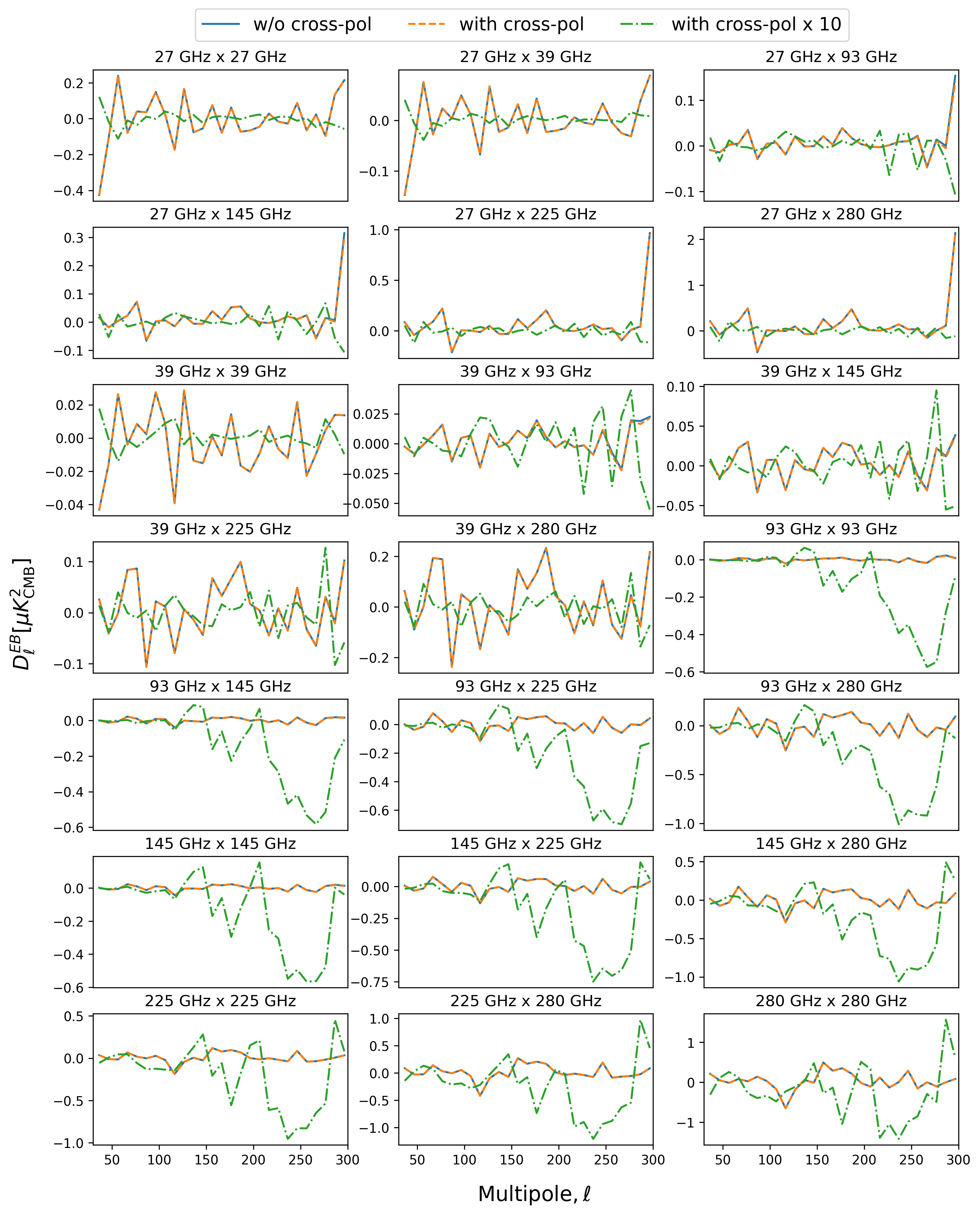
As discussed in Section 4.1, the component separation analysis results do not seem to vary significantly when introducing the cross-polar component of the simulated beam. Nevertheless, it is important to assess the cross-polarization impact on the resulting spectra. A rotation of the spectra due to cross-polarization could interfere with cosmic birefringence measurements or affect the polarization angle calibration [15]. In contrast to beam asymmetry, the effect of beam cross-polarization can not be mitigated in the case where a HWP is included in the instrumental setup [16]. Figure 9 shows the auto- and cross-channel spectra estimated from six center-frequency beamconv maps of a single sky realization with NaMaster. In the case of MF and UHF bands, the maps have been convolved either with strictly co-polar beams (blue) or with beams carrying both the co- and cross-polar components. The LF beams are still approximated with Gaussian distributions. We run simulations using both the cross-polar beams generated with TICRA TOOLS (orange) and a modified version, where the cross-polarization amplitude is intentionally exaggerated by an order of magnitude (green) for comparison.
The sky maps, whose spectra are shown in this figure, consist of CMB and Gaussian foregrounds. They have been masked and corrected for mode-mixing. While it would be more appropriate to use simulations of a CMB-only sky model for this assessment, the spectra convolved with beams that include the unscaled cross-polarization component appear identical to those convolved with only co-polar beams. Non-negligible values for these two cases are observed only due to foregrounds and cut-sky effects. The contribution of foregrounds to the spectra of maps convolved with either co-polar beams or beams that include the nominal cross-polar component becomes apparent when examining their auto-spectra. Notably, the spectra from the lowest () and highest frequency channels () exhibit the largest amplitudes. The MF channels ( and ), which refer to the least foreground-contaminated frequency regime, exhibit spectra amplitudes on the order of and do not appear to deviate significantly from the spectra shown in [33]. To quantify any systematic -to- leakage from beamconv simulations, the best-fit birefringence angle will be estimated in the near future from maps that do not contain any foreground emission.
When we scale up the amplitude of the cross-polar beam by an order of magnitude we observe the correlation notably increasing, in particular for the highest frequencies. After the scaling, the cross-polar beam becomes roughly just an order of magnitude fainter than the co-polar beam, resulting in some -to- leakage in the power spectra, primarily impacting the higher multipoles. The degree-scale spectra, where -modes are expected to peak, do not appear to be significantly threatened by this (large) increase in the cross-polarization amplitude.
Appendix C Dependence on the detector location
The beam model depends on the position of the detector on the telescope’s focal plane. A detector positioned at the edge of the SAT focal plane produces a significantly more elliptical beam pattern compared to a detector placed on the boresight, due to the asymmetrical illumination of the telescope aperture. Specifically, SAT beam simulations indicate a variation in beam size and nearly a increase in beam ellipticity between the center and edge pixel cases [12]. Figure 10 shows the logarithmic beam profiles of two detectors located at the boresight and edge of the simulated SAT focal plane for the center frequencies of the MF and UHF frequency bands, which have been uniformly averaged over the beam azimuthal angle, . Upon examining the various sub-panels of this figure, we deduce that the edge-pixel beam profiles appear more diffuse compared to the sharper main peaks we see for the center pixels. Note that for this test, we use the narrow edge-pixel beams (extending to ) to achieve a direct comparison with the analysis described in Section 4.2.2 where the input beam models were simulated for boresight pixels only.
Applying the same component separation method on the -mode spectra of non-Gaussian foreground maps, which have been convolved with edge-pixel beam models, yields parameter values that closely match those presented in Table 3. The most significantly affected parameter is , for which the beam chromaticity bias is now estimated as 0.13, compared to just 0.01 in the center-pixel case. This minor difference, however, may not fully capture the realistic scenario, as the pixels at the edges of the SAT focal plane could also experience additional sidelobe power due to reflections from filters and other surface elements of the optical setup, which are not accounted for in the simulations.
Appendix D Chromaticity bias for different beam spectral response
Let us now assume that we have underestimated the intrinsic beam frequency scaling. In the simplest parametrization, we only account for the main beam which we describe solely by its best-fit FWHM. Specifically, we fit a first-order polynomial to the beam sizes of the five monochromatic frequencies employed for the MF and UHF frequency bands. We then increase the fitted slope by and by an exaggerated with respect to its original value while keeping the FWHM value of the center frequency of each band fixed. In this way, we increase the relative beam size difference inside the bands with respect to the corresponding band centers. We run beamconv simulations for the two newly constructed cases employing Gaussian beams and assuming Gaussian foregrounds. Table 4 presents the best-fit parameters in the cases where the beam spectral slope increases by and , averaged over ten sky realizations. The corresponding parameters for the nominal assumed spectral dependence of the beam are also shown as a reference, along with their input values.
| Parameter | Input | Chromatic | Chromatic | Chromatic |
|---|---|---|---|---|
| 1 | ||||
| 0 | ||||
| 1.54 | ||||
| 0 | ||||
| -0.16 | ||||
| 28 | ||||
| -3.0 | ||||
| -0.93 | ||||
| 1.6 |
For the more reasonable case of the increase in chromaticity, we observe the largest biases in the synchrotron parameters. This is due to the component separation algorithm assigning the additional frequency scaling to errors in the assumed spectral dependence of synchrotron which more closely resembles the scaled spectral dependence of the beam than does that of dust. On the other hand, for the exaggerated case of , it becomes evident that we can no longer recover the lensing amplitude and foreground parameters. The scaled beam spectral dependence is now very different from the ones of both dust and synchrotron and, thus, the code can not properly integrate it in the fitting model. The spectral indices of dust and synchrotron absorb most of the chromaticity bias. The tensor-to-scalar ratio increases in the first case (corresponding to a bias of compared to achromatic beams), yet remains largely unaffected in the second. Note that, even though we assumed Gaussian beams, we did the beam-convolution in the time-domain for consistency in the used method and associated biases throughout the paper.