vS-Graphs: Integrating Visual SLAM and Situational Graphs through Multi-level Scene Understanding

Abstract

Current Visual Simultaneous Localization and Mapping (VSLAM) systems often struggle to create maps that are both semantically rich and easily interpretable. While incorporating semantic scene knowledge aids in building richer maps with contextual associations among mapped objects, representing them in structured formats like scene graphs has not been widely addressed, encountering complex map comprehension and limited scalability. This paper introduces vS-Graphs, a novel real-time VSLAM framework that integrates vision-based scene understanding with map reconstruction and comprehensible graph-based representation. The framework infers structural elements (i.e., rooms and corridors) from detected building components (i.e., walls and ground surfaces) and incorporates them into optimizable 3D scene graphs. This solution enhances the reconstructed map’s semantic richness, comprehensibility, and localization accuracy. Extensive experiments on standard benchmarks and real-world datasets demonstrate that vS-Graphs outperforms state-of-the-art VSLAM methods, reducing trajectory error by an average of $\mathbf{3.38\%}$ and up to $\mathbf{9.58\%}$ on real-world data. Furthermore, the proposed framework achieves environment-driven semantic entity detection accuracy comparable to precise LiDAR-based frameworks using only visual features.

A web page containing more media and evaluation outcomes is available on https://snt-arg.github.io/vsgraphs-results/.

1 Introduction

Robust environment understanding, a core foundation of robots’ situational awareness when studied in the context of Simultaneous Localization and Mapping (SLAM) [1], relies heavily on the quality and type of sensor data. While various sensing modalities (e.g., Light Detection And Ranging (LiDAR) and cameras) have been employed in SLAM, vision sensors offer a cost-effective solution to guarantee rich map reconstruction, forming a distinct category titled Visual SLAM (VSLAM) [2]. Among vision sensors, RGB-D cameras offer rich fusions of visual and depth information. Such sensors address the limitations of monocular cameras and LiDARs, generating dense point clouds to provide detailed spatial information, precise detection, localization, and mapping of environmental elements [3]. To enhance VSLAM capabilities, computer vision techniques are integrated, ranging from semantic scene understanding algorithms [4] to incorporating artificial landmarks like ArUco markers [5].

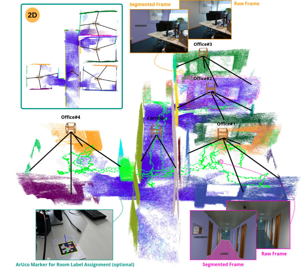
Figure 1: A reconstructed map tailored to the optimizable scene graph generated by the proposed vS-Graphs, enriched with environment-driven semantic entities.

Besides the benefits of enriching the map with visual and depth data, various methodologies can be used to organize the data into comprehensible structures. Among them, scene graphs are structured representations of scanned environments that record the presence of “objects,” their properties, and the intra-relationships. They secure a higher level of abstraction for scene understanding, generating hierarchical (i.e., graph-based) environment representations that outline spatial associations among observed objects [6]. While works like [7, 8] focus on tailoring geometric and semantic information for reliable environment interpretation, others like S-Graphs[9] push the boundaries by incorporating the scene graphs directly into SLAM. While S-Graphs employs LiDAR odometry with planar surface extraction within a unified optimization system, Hydra [10], builds 3D scene graphs in real-time from given sensor data (i.e., camera poses and point clouds).

Inspired by S-Graphs[9], this paper proposes a real-time VSLAM framework, titled visual S-Graphs (vS-Graphs), that integrates scene graph generation directly into the SLAM process. vS-Graphs is a real-time system that utilizes visual and depth data to enhance map reconstruction and camera pose estimation. It reliably incorporates “building components” (i.e., wall and ground surfaces), “structural elements” (i.e., rooms and corridors), and their associations into the reconstructed map for a more precise and structured representation of the environment. Consequently, it leverages detected building components as lower-level, environment-driven semantic entities to identify potential structural elements, thereby improving the VSLAM system’s accuracy by imposing additional semantic constraints. Ultimately, vS-Graphs generates comprehensible 3D scene graphs with hierarchical optimization capabilities that pair robot poses from the underlying SLAM with detected entities, as depicted in Fig. 1. It can also utilize fiducial markers (if present) to augment meta-data into the detected structural elements.

With this, the primary contributions of the paper are summarized below:

• A real-time multi-threaded VSLAM framework that generates hierarchical optimizable 3D scene graphs while reconstructing the map,

• A vision-based methodology for recognizing and mapping building components (i.e., wall and ground surfaces), enhancing map richness and reducing trajectory errors; and

• A solution for extracting high-level structural elements (i.e., rooms and corridors) from the localized building components for improved scene understanding.

2 Related Works

Recent advances in computer vision algorithms and the emergence of reliable VSLAM baseline frameworks like ORB-SLAM 3.0 [11] have enabled the development of more robust VSLAM systems. Considering the directions of VSLAM methods highlighted in [12], depth data can significantly enhance scene understanding, forming the basis for subsequent tasks like efficient environment modeling. In this regard, ElasticFusion [13] constructs globally consistent surfel-based maps for richer rendering and accurate photometric tracking. However, it faces challenges in scalability and optimal incorporation of environment-driven information. BAD SLAM [14] targets map and camera trajectory optimization through fast direct Bundle Adjustment (BA) using RGB-D data, yet it remains highly sensitive to initial pose estimates. More recent approaches, including GS-SLAM [15], RTG-SLAM [16], and SplaTAM [17], integrate 3D Gaussian scene representations into RGB-D rendering to enhance tracking accuracy and map reconstruction efficiency. Nonetheless, these methods overlook the integration of semantic information extracted from the scene during the mapping process.

Several RGB-D point cloud-based VSLAM systems have adopted semantic scene understanding into their mapping processes. Voxblox++ [18] integrates volumetric object-centric maps during online scanning to recognize and localize scene elements. Similarly, NICE-SLAM [19] combines neural implicit and hierarchical scene representations within a dense RGB-D VSLAM framework, utilizing pre-trained geometric priors to achieve improved scene reconstruction. Yet, these techniques often struggle with computational overhead and high localization errors. To address semantic awareness, works like SaD-SLAM [20], OVD-SLAM [21], and YDD-SLAM [22] use Convolutional Neural Networks to detect and filter feature points associated with specific semantic objects, refining pose estimation and trajectory accuracy. Additionally, the work in [23] introduces a binary CNN-based descriptor for robust feature detection and matching while improving the initial pose measurements. Despite these advancements, these approaches focus on object-level filtering or reconstruction rather than generating comprehensive scene representations enriched with environment-driven entities.

Another direction involves using fiducial markers as reliable landmarks within the environment, offering an alternative to purely computer vision-based scene interpretation. Techniques such as [24, 25] detect and map environment-driven entities labeled with fiducial markers that contribute to a more comprehensive understanding of the environment layout. Nevertheless, their reliance on pre-placed markers limits their applicability to controlled environments, reducing flexibility in unprepared or dynamic settings.

In contrast with the reviewed literature, vS-Graphs is a real-time VSLAM that integrates 3D scene graph construction into the SLAM, enhancing mapping accuracy and trajectory estimation while providing semantically rich environment representations, all without requiring augmented landmarks (e.g., markers).

3 Proposed Method

3.1 System Overview

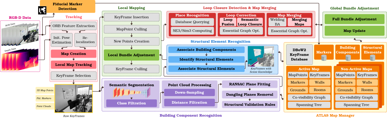
Figure 2: The multi-thread architecture of vS-Graphs. Modules with dashed borders and a light gray background are inherited directly from the baseline (i.e., ORB-SLAM 3.0), while the remaining components are newly added or modified modules.

Building upon ORB-SLAM 3.0, vS-Graphs introduces substantial modifications to its baseline’s core modules and adds new threads for robust scene analysis and reconstruction. The system architecture, shown in Fig. 2, details the individual threads, components, and their interconnections. The current version supports RGB-D feed, employing the depth data for robust scene understanding. The core contribution lies in seamlessly integrating two novel threads: “Building Component Recognition” (3.2) and “Structural Element Recognition” (3.3). These threads are tightly integrated within vS-Graphs, triggered by other threads for enriching the reconstructed maps and optimal performance.

At the core, RGB-D data processing is performed in real-time, supplying visual and depth information. Concurrently, “Fiducial Marker Detection” (ArUco [5] library in this work) runs independently on the input frames to detect potential markers and store their unique identifier and pose in the map manager, Atlas. Visual features are extracted and tracked across sequential frames in the “Tracking” thread. In this thread, pose information is either initialized or refined, depending on the map reconstruction stage, creating a 3D map with tracked features across frames. Finally, KeyFrame selection, a critical step following feature extraction, is performed by analyzing the visual data. These KeyFrames contain 3D map points, point clouds, and potentially detected fiducial markers, forming the foundation for subsequent processes.

KeyFrames are then sent to the “Local Mapping” thread for map integration and optimization, with inaccurately posed KeyFrames culled for enhanced accuracy. Simultaneously, the “Building Component Recognition” thread identifies and localizes walls and ground surfaces by processing the KeyFrame-level point clouds. In another thread, “Structural Element Recognition” runs in constant intervals, extracting higher-level entities, including rooms and corridors, from the active map. Ultimately, and owing to the “Loop Closure Detection”, the system corrects or merges the map if the current location has been revisited and triggers “Global Bundle Adjustment” for map optimization when a loop is detected.

3.2 Building Component Recognition

This thread processes the point cloud and visual data from KeyFrames to extract environment-driven and fundamental elements beneficial for scene understanding. The current version of vS-Graphs defines building components as walls and ground surfaces. Accordingly, each KeyFrame $K=\{\mathbf{P},L,\upsilon\}$ passes through the building component recognition module $B$, generating identified structural elements set $\mathbf{\Pi}_{\mathbf{\Psi}}^{K}=B(\mathbf{K})$ for the KeyFrame $K$. In the KeyFrame level, $\mathbf{P}=\{p_{i}~|~p\in\mathbb{R}^{3},i\in\mathbb{N}\}$ is the point cloud, $L$ is the matrix of RGB data, and $\upsilon$ represents additional metadata for mapping such as camera pose.

Building component extraction is achieved by processing $L$ through a semantic segmentation function $S$, which labels each pixel in the RGB data, retaining only the relevant classes and discarding irrelevant entities. Since a real-time panoptic semantic segmentation framework is required to offer sharper boundary detection and effective differentiation among objects within the same class, YOSO [26] is integrated into vS-Graphs. In this regard, $\widehat{\mathbf{P}}_{\mathbf{\Psi}}^{K}=S(\mathbf{P},L)$ refers to the segmented visual-spatial data of $K$, where $L_{(x,y)}$ refers to the semantic class label of a pixel at $(x,y)\in\mathbb{N}^{2}$. Applying semantic class filtration to filter building components’ semantic classes $\mathbf{\Psi}$ (i.e., wall and ground surfaces) takes place as follows:

$$\widehat{\mathbf{P}}_{\psi}^{K}=\{p_{j}~|~p_{j}=(x,y,z)\in\mathbb{R}^{3},L_{p_{j}}\in\mathbf{\Psi}\}$$ (1)

$$\widehat{\mathbf{P}}_{\mathbf{\Psi}}^{K}=\{\widehat{\mathbf{P}}_{\psi}^{K}\}=\{\widehat{\mathbf{P}}_{wall}^{K},\widehat{\mathbf{P}}_{ground}^{K}\}$$ (2)

where $\widehat{\mathbf{P}}_{\mathbf{\Psi}}^{K}\subset\mathbf{P}$ represents the set of semantically segmented point clouds, including the point clouds of $\widehat{\mathbf{P}}_{wall}^{K}$ and $\widehat{\mathbf{P}}_{ground}^{K}$. It should be noted that the uncertainty parameter $\lambda_{(x,y)}\in\mathbb{R}$ for each pixel ${L_{\Psi}}_{(x,y)}$ is also considered for potential classification errors.

The next stage is to optimize $\widehat{\mathbf{P}}_{\mathbf{\Psi}}^{K}$, as it may contain noisy or low-resolution points that negatively impact subsequent steps. In this regard, each segmented visual-spatial point cloud $\widehat{\mathbf{P}}_{\psi}^{K}$ undergoes a two-stage preprocessing procedure. The first step is applying down-sampling to fetch $\widehat{\mathbf{P}}_{{\psi}_{d}}^{K}$, a refined point cloud with reduced redundancy and noise, where $\widehat{\mathbf{P}}_{{\psi}_{d}}^{K}\subset\widehat{\mathbf{P}}_{\psi}^{K}$. The subsequent step involves distance filtration on $\widehat{\mathbf{P}}_{{\psi}_{d}}^{K}$, retaining only the points that satisfy the condition $\widehat{\mathbf{P}}_{{\psi}_{\zeta}}^{K}=\{p_{\zeta}\in\widehat{\mathbf{P}}_{{\psi}_{d}}^{K}~|~{\theta}_{min}\leq\|p_{\zeta}\|\leq{\theta}_{max}\}$, where ${\theta}_{min}$ and ${\theta}_{max}$ are minimum and maximum desired depth thresholds, respectively. The final processed point cloud, referred to as $\widehat{\mathbf{P}}_{\mathbf{{\Psi}_{\zeta}}}^{K}=\{\widehat{\mathbf{P}}_{{\psi}_{\zeta}}^{K}\}$, is then forwarded to successive stages for further analysis.

Processing each $\widehat{\mathbf{P}}_{{\psi}_{\zeta}}^{K}$ through RANdom SAmple Consensus (RANSAC) [27] plane fitting algorithm results in detecting semantically-validated building components with their geometric equations. Thus, sets of random points $\mathbf{p_{r}}\in\widehat{\mathbf{P}}_{{\psi}_{\zeta}}^{K}$ are iteratively selected to calculate the normal vectors $\mathbf{n}\in\mathbb{R}^{3}$ representing validated planar components $\mathbf{\pi}$ with the pre-defined distance $d(\mathbf{{p_{r}}},\pi)\leq\epsilon$, where $\epsilon$ is the inlier threshold. Accordingly, the final output representing all defined building components is as follows:

$$\mathbf{\Pi}_{\psi}^{K}=\{{\pi_{\psi}}_{m}^{K}~|~{\pi_{\psi}}_{m}^{K}\in\mathbb{R}^{3},m\in\mathbb{N}\}$$ (3)

$$\mathbf{\Pi}_{\mathbf{\Psi}}^{K}=\{\mathbf{\Pi}_{\psi}^{K}\}=\{\mathbf{\Pi}_{wall}^{K},\mathbf{\Pi}_{ground}^{K}\}$$ (4)

The remaining reliable elements are checked against structural validation rules $\mathbf{\Pi}_{\mathbf{\Psi}}^{K}=V(\mathbf{\Pi}_{\mathbf{\Psi}}^{K})$, ensuring that they satisfy reasonable geometric constraints for the environment. For instance, walls should be represented as vertical planes, while ground surfaces must be horizontal. The thread concludes the processing of KeyFrame $K$ by storing its detected building components $\mathbf{\Pi}_{\mathbf{\Psi}}^{K}$ within the current map in the Atlas, ensuring they contribute to the ongoing map reconstruction.

3.3 Structural Element Recognition

This thread is repeatedly run at constant time intervals (i.e., every two seconds) to detect potential higher-level semantic entities that characterize the environment’s layout, including rooms and corridors. Structural elements comprise multiple building components, with their topological associations considered. The thread actively searches for layouts forming corridors or rooms: a corridor is defined by two parallel walls facing each other along with a ground surface, while a room is identified by four walls arranged in two pairs of parallel, opposing walls, all enclosing a ground surface.

In the first step, the map’s existing building components $\mathbf{\Pi}_{\mathbf{\Psi}}=\{\mathbf{\Pi}_{\mathbf{\Psi}}^{K_{i}}~|~i\in\mathbb{N}\}$ are fetched from Atlas. Associating and merging redundant or conflicting building components is crucial to ensure consistency in the map reconstruction. In this context, the primary factors to assess are the spatial proximity and alignment of the mapped building components, requiring evaluating both the Euclidean distance and the angular difference between their normal vectors. Accordingly, the building component association condition is presented below:

$$\|\mathbf{\Pi}_{\mathbf{\Psi}}^{K_{i}}-\mathbf{\Pi}_{\mathbf{\Psi}}^{K_{j}}\|\leq\rho\quad\text{\&}\quad\cos^{-1}\left(\frac{\mathbf{n}_{i}\cdot\mathbf{n}_{j}}{\|\mathbf{n}_{i}\|\|\mathbf{n}_{j}\|}\right)\leq\eta$$ (5)

where $\mathbf{n}$ is the normal vectors of a particular surface and $\rho$ and $\eta$ refer to spatial proximity and angular alignment thresholds, respectively. The associated building components $\mathbf{\Pi}_{\mathbf{\Psi}}$ are subsequently utilized to detect structural elements $\mathbf{\Delta}_{\mathbf{\Phi}}$, defined as below:

$$\mathbf{\Delta}_{\phi}^{K}=\{{\delta_{\phi}}_{m}^{K}~|~{\delta_{\phi}}_{m}^{K}\in\mathbb{R}^{3},m\in\mathbb{N}\}$$ (6)

$$\mathbf{\Delta}_{\mathbf{\Phi}}^{K}=\{\mathbf{\Delta}_{\phi}^{K}\}=\{\mathbf{\Delta}_{corridor}^{K},\mathbf{\Delta}_{room}^{K}\}$$ (7)

where $\mathbf{\Delta}_{\mathbf{\Phi}}^{K}\in\mathbf{\Delta}_{\mathbf{\Phi}}$ is the set of structural elements belong to semantic classes $\mathbf{\Phi}$ found in KeyFrame $K$. The structural element detection procedure is outlined below.

Corridors. A corridor $\delta_{c}^{K}=\{\mathbf{\Pi}_{wall},{\pi_{ground}^{K_{q}}},\mathbf{\nu}_{c}\}$ in the global reference frame $G_{t}$ is a space characterized by two walls $\mathbf{\Pi}_{wall}$ and a ground plane ${\pi_{ground}^{K_{q}}}$ oriented perpendicularly to them. In $\mathbf{\Pi}_{wall}=\{\pi_{wall}^{K_{i}},\pi_{wall}^{K_{j}}\}$, the normal vectors are facing each other, approximately parallel within a predefined angular threshold $\vartheta$, expressed as $\mathbf{n}_{wall}^{K_{i}}\cdot\mathbf{n}_{wall}^{K_{j}}\geq\cos(\vartheta)$. To detect the centroid of the corridor, first, a midpoint $\mathbf{k}_{c}$ between the two walls of $\mathbf{\Pi}_{wall}$ is calculated as below:

$$\mathbf{k}_{c}=\frac{1}{2}[\lvert{{d_{\pi_{wall}^{K_{i}}}}\rvert}\cdot{\mathbf{n}_{\pi_{wall}^{K_{i}}}}-{\lvert{d_{\pi_{wall}^{K_{j}}}}\rvert}\cdot{\mathbf{n}_{\pi_{wall}^{K_{j}}}}]+\lvert{{d_{\pi_{wall}^{K_{j}}}}\rvert}\cdot{\mathbf{n}_{\pi_{wall}^{K_{j}}}}$$ (8)

where $d$ and $\mathbf{n}$ are the given wall’s distance from the origin of $G_{t}$ and its normal vector, respectively. Then, the corridor’s geometric centroid $\mathbf{\nu}_{c}\in\mathbb{R}^{3}$ is calculated as:

$$\mathbf{\nu}_{c}=\mathbf{k}_{c}+(\varrho_{w}-[\ \varrho_{w}\cdot\hat{{\mathbf{k}}_{c}}])\cdot\hat{{\mathbf{k}}_{c}})$$ (9)

where ${\hat{\mathbf{k}}_{c}}={\mathbf{k}_{c}}/\|{\mathbf{k}_{c}}\|$ and $\varrho_{w}$ is the arithmetic mean of all points in one of the walls’ point cloud. Additionally, the ground plane $\pi_{ground}^{K_{q}}$ is associated with $\delta_{c}^{K}$ if it satisfies the conditions below, ensuring that $\pi_{ground}^{K_{q}}$ is perpendicular to $\mathbf{\Pi}_{wall}$ and its centroid $\varrho_{g}$ is located between them:

$$\mathbf{n}_{ground}\cdot\mathbf{n}_{wall}^{K_{i}}\leq\sin(\vartheta)\quad\text{\&}\quad\mathbf{n}_{ground}\cdot\mathbf{n}_{wall}^{K_{j}}\leq\sin(\vartheta)$$ (10)

$$d_{\pi_{wall}^{K_{i}}}\leq\varrho_{g}\leq d_{\pi_{wall}^{K_{j}}}$$ (11)

The cost function to minimize the corridor’s vertex node and its corresponding wall and ground surfaces is as follows:

$$c_{\delta_{c}^{K}}=\sum_{t=1}^{T}\|\hat{\mathbf{\nu}_{c}}-f(\pi_{wall}^{K_{i}},\pi_{wall}^{K_{j}},{\pi_{ground}^{K_{q}}},\varrho_{w},\varrho_{g})\|^{2}_{\mathbf{\Lambda}_{\mathbf{\tilde{\delta}}_{c,t}}}$$ (12)

where $f(\dots)$ is a mapping function that associates the building components with the corridor’s center point.
Rooms. A room $\delta_{r}^{K}=\{\mathbf{\Pi}_{wall},{\pi_{ground}^{K_{q}}},\mathbf{\nu}_{r}\}$ extends the concept of a corridor to a rectangular space, defined by four walls arranged in pairs of parallel surfaces, rather than just two. In $\mathbf{\Pi}_{wall}=\{\mathbf{\Pi}_{p_{1}},\mathbf{\Pi}_{p_{2}}\}=\{\{\pi_{wall}^{K_{i}},\pi_{wall}^{K_{j}}\},\{\pi_{wall}^{K_{u}},\pi_{wall}^{K_{v}}\}\}$ the normal vectors of each inner pair of walls are facing each other, defining them approximately parallel within an angular threshold $\vartheta$:

$$\mathbf{n}_{wall}^{a}\cdot\mathbf{n}_{wall}^{b}\geq\cos(\vartheta)\quad\text{\&}\quad|\mathbf{n}_{wall}^{a}\cdot\mathbf{n}_{wall}^{c}|\leq\sin(\vartheta)$$ (13)

where $\{a,b\}\in p_{1}$, $c\in p_{2}$, and $\mathbf{n}$ represents the normal vector of a wall. The room’s centroid $\mathbf{\nu}_{r}$ is computed similarly to the midpoint calculation for two intersecting corridors. Thus, equation 8 must be applied twice—once for each wall pair, resulting in two midpoints $\mathbf{k}_{c_{1}}$ for $\mathbf{\Pi}_{p_{1}}$ and $\mathbf{k}_{c_{2}}$ for $\mathbf{\Pi}_{p_{2}}$. The arithmetic mean of these two midpoints is the room centroid $\mathbf{\nu}_{r}=\frac{1}{2}\left(\mathbf{k}_{c_{1}}+\mathbf{k}_{c_{2}}\right)$. The ground $\pi_{ground}^{K_{q}}$ to the room $\delta_{r}^{K}$ association is also similar to equations 10-11, considering that $\mathbf{n}_{ground}$ is approximately perpendicular to the normal vectors of the walls in both pairs. Moreover, the cost function to minimize the room’s vertex node and its corresponding wall and ground surfaces is as follows:

$$c_{\delta_{r}^{K}}=\sum_{t=1}^{T}\|\hat{\mathbf{\nu}_{r}}-f(\mathbf{\Pi}_{p_{1}},\mathbf{\Pi}_{p_{2}},{\pi_{ground}^{K_{q}}},\varrho_{w},\varrho_{g})\|^{2}_{\mathbf{\Lambda}_{\mathbf{\tilde{\delta}}_{r,t}}}$$ (14)

where $f(\dots)$ is a mapping function that associates the building components with the room’s center point.

3.4 Marker-based Semantic Augmentation

In vS-Graphs, fiducial markers augment structural elements with indirect high-level semantic information, helping contextualize the environment by coupling additional data (e.g., room names) to interpret the reconstructed map meaningfully. Unlike [25, 24], where markers play a prominent role in map reconstruction, their function here is less critical. Instead, they grant high-value semantic enrichment without the map being dependent on their presence.

Accordingly, each fiducial marker $\mathbf{m}_{i}^{K}=\{\mathbf{p}_{m},\mathbf{\nu}_{m}\}$ in $G_{t}$ is constrained by the KeyFrame $K$ observing it, where $\mathbf{p}_{m}\in SE(3)$ is the marker’s pose and $\mathbf{\nu}_{m}$ is its center point. The mentioned constraint is defined below:

$$\mathbf{\sigma}_{m}(^{G}\mathbf{K},\mathbf{m}_{i}^{K})=\|^{L}\mathbf{m}_{i}\boxplus\leftidx{{}^{G}}{\mathbf{K}}\boxminus\leftidx{{}^{G}}{\mathbf{m}_{{i_{1}}}}\|^{2}_{\mathbf{\Lambda}_{\mathbf{\tilde{m}}_{i}}}$$ (15)

where ${}^{L}\mathbf{m}_{{i}}$ refers to the locally observed marker’s pose, $\boxplus$ and $\boxminus$ represent the composition and inverse composition, $\|\dots\|$ is the Mahalanobis distance, and $\mathbf{\Lambda}_{\mathbf{\tilde{m}}_{i}}$ is marker’s information matrix.

The marker $\mathbf{m}_{i}^{K_{j}}\in\mathbf{M}$ is associated with a structural element if it lies within the spatial bounds of the detected room/corridor $\delta^{K_{g}}\in\mathbf{\Delta}_{\phi}$. Thus, the Euclidean distance between the center point $\mathbf{\nu}_{m}$ of $\mathbf{m}_{i}^{K_{j}}$ and the room/corridor’s centroid $\mathbf{\nu}_{s}$, expressed as $d(\mathbf{\nu}_{m},\mathbf{\nu}_{s})\leq\epsilon_{s}$, where $\epsilon_{s}$ is the proximity threshold. The supporting condition is that $\mathbf{\nu}_{m}$ must be enclosed among all bounding walls $\mathbf{\Pi}_{wall}$ with the normal vector $\mathbf{n}$

$$\forall\pi_{wall}^{K_{i}}\in\mathbf{\Pi}_{wall},\quad(\mathbf{n}_{wall}^{K_{i}}\cdot(\mathbf{\nu}_{m}-\mathbf{\nu}_{r}))\leq 0$$ (16)

3.5 Scene Graph Structure

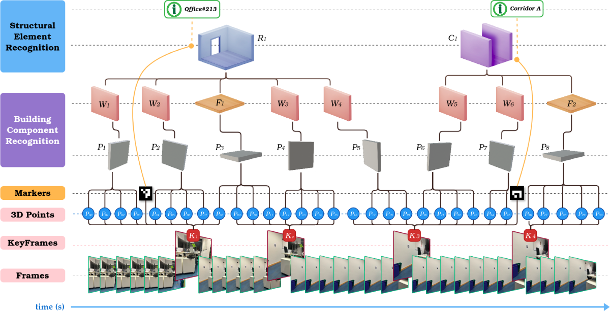
Figure 3: Scene graph structure generated using vS-Graphs, creating a hierarchical representation of the environment.

Fig. 3 depicts the 3D scene graph structure generated using vS-Graphs, along with its corresponding modules introduced in Fig. 2. In contrast to the traditional SLAM reconstructed maps, the geometric replicas of vS-Graphs are augmented with hierarchical rich semantic data, enabling meaningful interaction with the environment. The generated scene graph fills the contextual understanding gap and supplies better scene interpretation, leading to complementary missions such as scalable map-building and improved decision-making.

4 Experimental Results

4.1 Evaluation Criteria

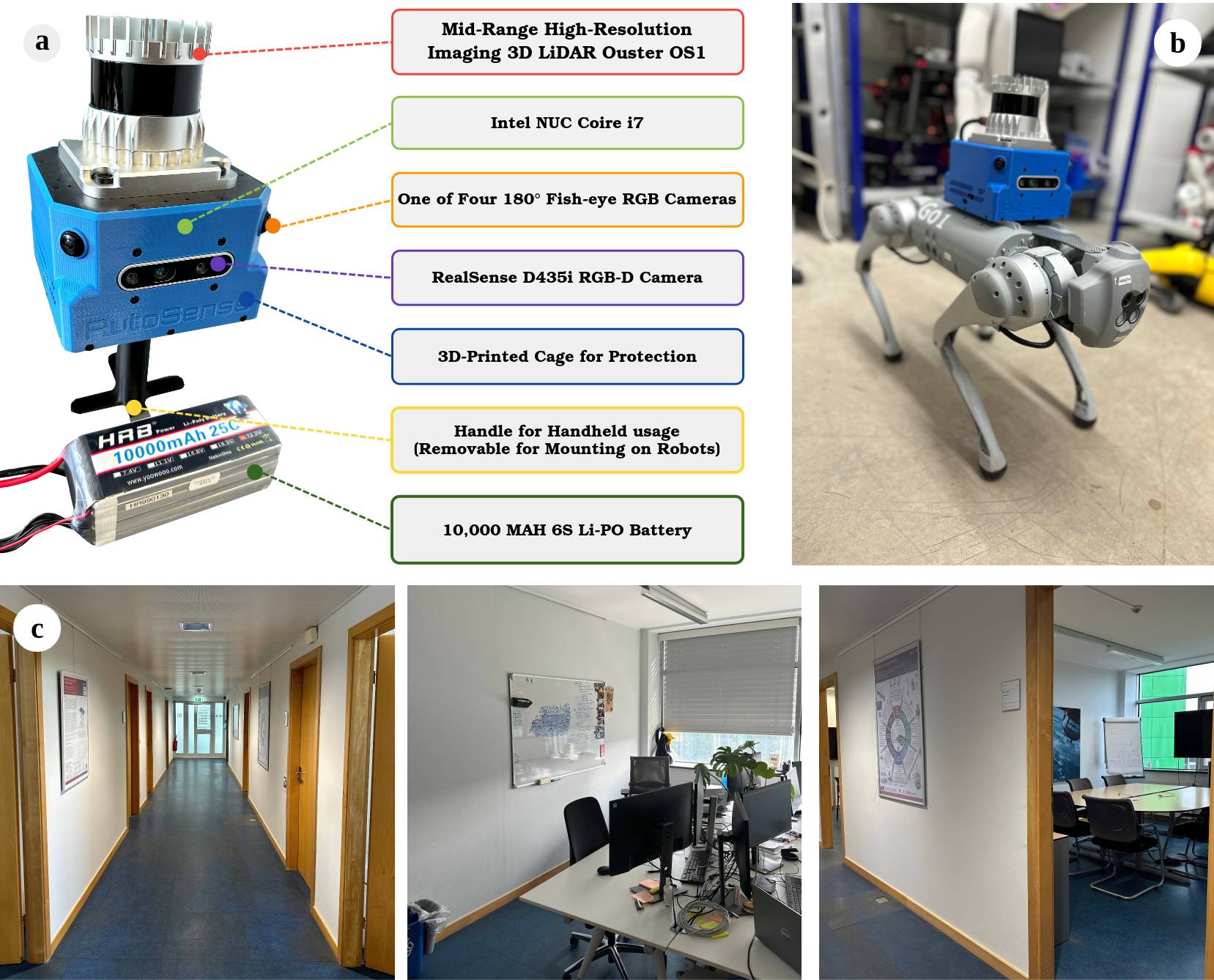
Figure 4: In-house dataset collection using the AutoSense device: a) the setup overview, b) the device mounted on a legged robot, and c) some instances of the collected data.

Evaluations were conducted on a system with an Intel® Core™ i9-11950H processor (2.60 GHz), a 4GB NVIDIA T600 Mobile GPU, and 32GB of RAM. vS-Graphs was assessed using both standard benchmarks (real and photorealistic) and proprietary in-house datasets. The in-house data was collected using a custom-built, handheld/robot-mountable device called AutoSense, which records RGB-D video alongside LiDAR point clouds. The collected AutoSense dataset contains sequences of diverse real-world indoor environments with varying architectural layouts, as shown in Fig. 4. ArUco fiducial markers [5] were strategically placed in some rooms to augment semantic information (i.e., room label). Additionally, the ground truth data in the dataset were obtained using reliable LiDAR poses and points cloud generated by S-Graphs. Due to space constraints, the complete evaluation results and figures are available at https://snt-arg.github.io/vsgraphs-results/.

4.2 Trajectory Estimation and Mapping Performance

Table 1: Absolute Trajectory Error (ATE) in meters for various VSLAM algorithms across eight iterations. The best and second-best results are boldfaced and underlined, respectively. The final column shows the percentage improvement of vS-Graphs over the baseline (ORB-SLAM 3.0).

Dataset			Methodologies
Sequence		Span	ORB-SLAM 3.0 [11]	BAD SLAM [14]	ElasticFusion [13]	vS-Graphs	Diff. (%)
ICL [28]	deer-gr	79.9	0.007	1.476	0.145	0.008	-8.89%
	deer-wh	65.3	0.070	-	0.825	0.061	+12.64%
	deer-w	64.0	0.099	1.474	0.620	0.088	+10.97%
	deer-r	28.4	0.069	-	0.787	0.053	+22.83%
	deer-mavf	102.5	0.027	0.046	-	0.026	+0.96%
OpenLORIS [29]	office1-1	27.0	0.064	0.123	0.069	0.064	-0.66%
	office1-2	30.0	0.101	0.140	0.113	0.099	+1.39%
	office1-3	12.0	0.147	0.195	-	0.146	+1.08%
	office1-4	29.0	0.125	0.343	0.180	0.127	-1.37%
	office1-5	53.0	0.116	0.302	0.221	0.111	+4.35%
	office1-6	36.5	0.059	0.107	-	0.059	-0.68%
	office1-7	38.6	0.172	0.203	-	0.175	-2.18%
ScanNet [30]	sc0041-01	75.0	0.143	0.222	0.220	0.143	-0.27%
	sc0200-00	37.0	0.049	-	-	0.047	+4.36%
	sc0614-01	36.2	0.135	0.139	0.202	0.125	+7.76%
	sc0626-00	21.1	0.096	0.273	0.189	0.095	+1.05%
TUM-RGBD [31]	frb1-desk	23.8	0.021	0.022	0.026	0.020	+4.25%
	frb1-desk2	25.1	0.032	0.029	0.079	0.032	+1.17%
	frb1-room	49.1	0.130	0.209	0.167	0.130	+1.75%
	frb2-desk	142.1	0.019	0.096	0.045	0.018	+5.69%
	frb3-strct	31.9	0.016	0.021	0.017	0.015	+5.04%
AutoSense (in-house)	room-walls	61.0	0.080	0.130	0.066	0.081	-1.58%
	room-corner	80.0	0.088	0.135	-	0.082	+6.15%
	single-room	170.0	0.109	0.557	-	0.107	+1.85%
	room-across	305.0	0.153	0.413	-	0.154	-1.13%
	room-corrdr	210.0	0.240	-	0.535	0.217	+9.58%
	office-suite	783.0	0.222	0.812	-	0.220	+0.87%
Total		48m 36s				Mean	+3.38%

To showcase vS-Graphs’s trajectory estimation accuracy, it was compared against ORB-SLAM 3.0 (baseline) [11], ElasticFusion [13], and BAD SLAM [14] due to their robustness and widespread use in VSLAM works. Marker-dependent (e.g., [24]) and neural field SLAM (such as [19]) methods were excluded from evaluations to ensure a direct comparison focused on the core performance of vS-Graphs. Accordingly, marker-based VSLAMs use external pose constraints and demand fiducial markers to incorporate semantic entities, limiting their applicability in marker-free data instances. Also, neural RGB-D methods rely on their learned scene priors and implicit representations, diverging from the proposed mapping strategy. Table 1 presents the evaluation results, with each system evaluated over eight runs on dataset instances, and performance was measured using Absolute Trajectory Error (ATE) reported in meters. Dashes in Table 1 indicate unavailable data due to failure in tracking.

According to the evaluation results, vS-Graphs consistently achieves state-of-the-art performance, securing the best or second-best results in almost all cases. This superior performance is particularly evident in the longer, real-world sequences, originating from integrating constraints derived from accurately localized building components and structural elements. While including these entities enhances trajectory estimation, inaccurate mapping and localizing them can negatively impact results. Such cases are mainly associated with rapid camera motion (seq. deer-gr) and noisy point cloud data (seq. office1-7). On average, vS-Graphs demonstrates a $3.38\%$ improvement over the baseline in all sequences.

Additionally, analyzing the accuracy of the reconstructed maps against AutoSense’s ground truth data revealed that vS-Graphs performs more robustly compared to ORB-SLAM 3.0 in terms of Root Mean Square Error (RMSE). As shown in Fig. 5, the median RMSE is consistently lower in vS-Graphs, indicating a higher level of overall mapping precision. vS-Graphs achieves superior mapping accuracy despite generating maps with $\sim 10.15\%$ fewer points on average than the baseline, owing to its environment-driven constraints that enable a more coherent reconstruction.

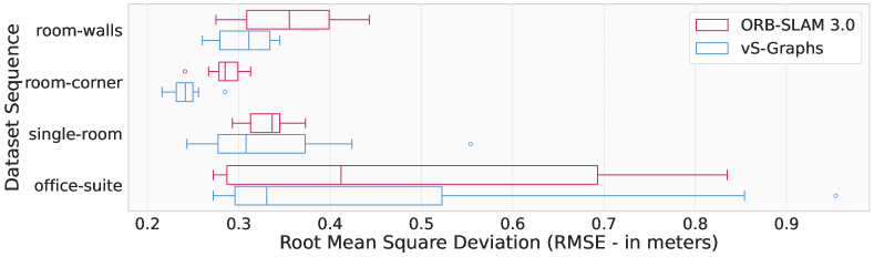
Figure 5: Mapping performance across eight iterations, showing AutoSense sequences with less than one meter RMSE.

4.3 Scene Understanding Performance

This section evaluates the performance of vS-Graphs in semantic scene understanding, explicitly accurately detecting the entities essential for interpreting the environment’s layout. To benchmark this capability, the sequences with multiple rooms from the AutoSense dataset were used, as they offer ground-truth annotations derived from LiDAR data. Table 2 presents a quantitative comparison of vS-Graphs against two state-of-the-art approaches: Hydra [10] and S-Graphs[9]. While S-Graphs benefits from the geometric precision of LiDAR point clouds, Hydra was configured to use visual point clouds, ensuring a fair comparison against our purely vision-based approach.

Experimental results demonstrate that vS-Graphs, despite relying solely on visual input, achieves an accuracy comparable to the LiDAR-based method in detecting building components and structural elements. This highlights the effectiveness of its visual feature processing and scene graph generation in comprehending the environment with high precision. It should be noted that “wall” entities are not directly provided in Hydra; therefore, Hydra’s performance is assessed based on correct “room” element counting and recognition. Additionally, the current implementation of vS-Graphs does not include “floor” entities, which is discarded from the analysis. Fig. 6 provides a qualitative comparison of the reconstructed scene graphs generated by vS-Graphs, S-Graphs, and Hydra across two dataset instances.

Table 2: Scene understanding accuracy on multi-room sequences of AutoSense dataset. BC and SE refer to “building components” and “structural elements,” respectively.

		Detected / Real		Precision		Recall
Method	Sequence	BC	SE	BC	SE	BC	SE
S-Graphs [9]	room-across	13 / 12	3 / 3	0.92	1.00	0.92	1.00
	room-corrdr	12 / 13	3 / 3	1.00	1.00	0.92	1.00
	office-suite	20 / 17	4 / 4	0.89	1.00	0.94	1.00
Hydra [10]	room-across	N/A	3 / 3	N/A	1.00	N/A	1.00
	room-corrdr	N/A	5 / 3	N/A	0.75	N/A	0.75
	office-suite	N/A	4 / 4	N/A	1.00	N/A	1.00
vS-Graphs (ours)	room-across	14 / 12	3 / 3	0.86	1.00	1.00	1.00
	room-corrdr	14 / 13	3 / 3	0.92	1.00	0.92	1.00
	office-suite	18 / 17	4 / 4	0.94	1.00	1.00	1.00

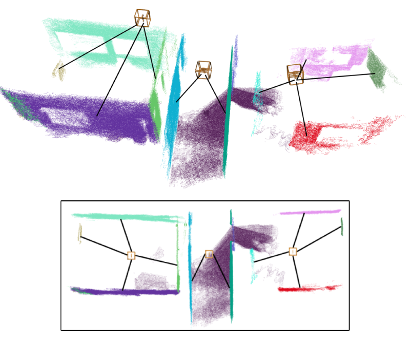
(a) vS-Graphs on room-across

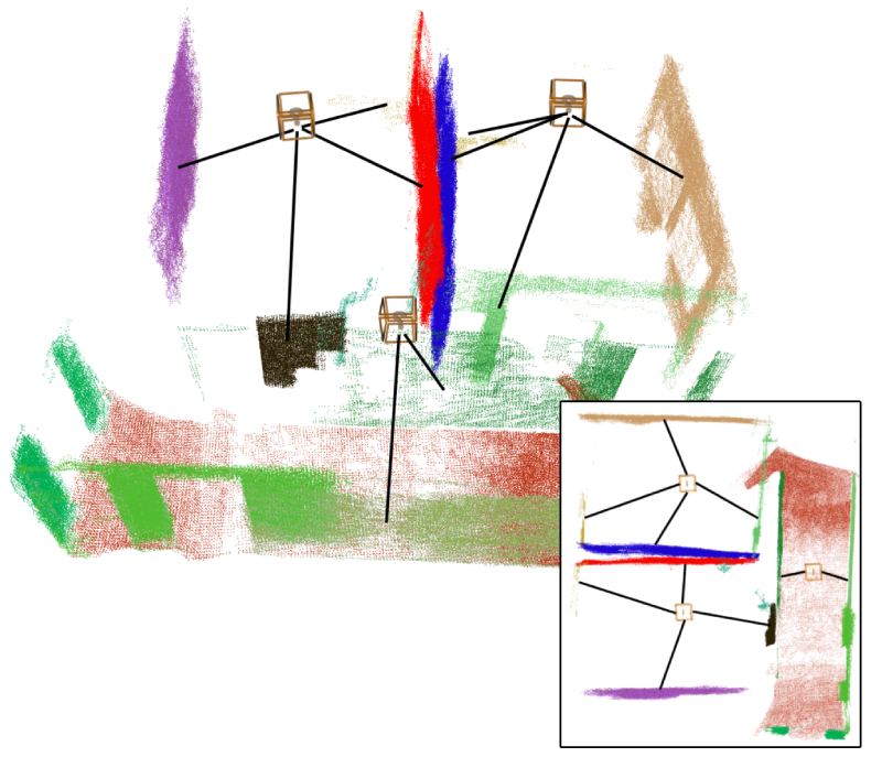
(b) vS-Graphs on room-corrdr

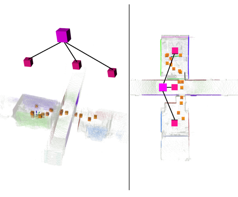
(c) S-Graphs on room-across

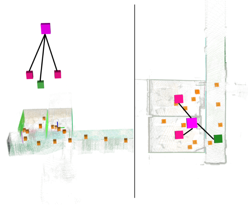
(d) S-Graphs on room-corrdr

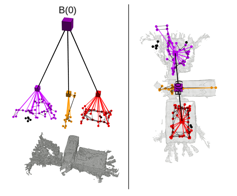
(e) Hydra on room-across

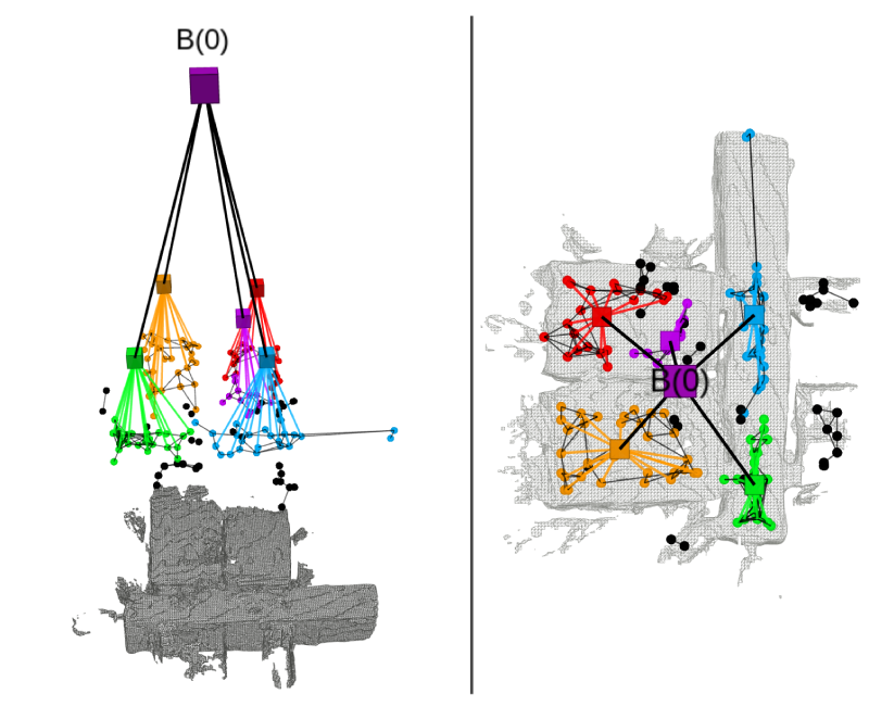
(f) Hydra on room-corrdr

Figure 6: Qualitative comparison of reconstructed scene graphs on multi-room sequences of the AutoSense dataset.

4.4 Runtime Analysis

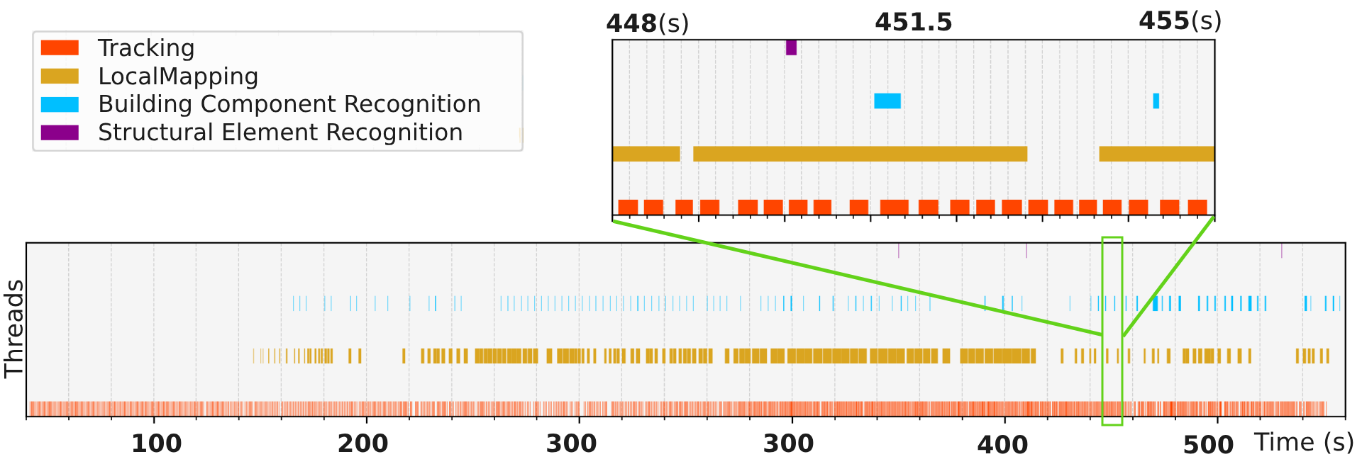
Figure 7: Timeline of thread execution within vS-Graphs while processing a sample dataset instance (sequence room-walls).

vS-Graphs achieves real-time performance with an average processing rate of $22\pm 3$ Frames per Second (FPS), exceeding the $20$ FPS threshold for real-time operation. This is accomplished through a multi-threaded architecture, as shown in Fig. 7. The “Tracking” thread processes visual features at frame level, while “Local Mapping” concurrently maps objects and optimizes their positions. “Building Component Recognition”, running in parallel at the KeyFrame level, identifies potential wall and ground surfaces from the online panoptic segmentation. The “Structural Element Recognition” runs less frequently and in constant periods (every two seconds) to infer rooms and corridors in the map. Compared to ORB-SLAM 3.0’s $29\pm 3$ FPS on the same hardware and dataset, the slightly reduced frame rate is a reasonable trade-off for vS-Graphs’s rich semantic scene understanding.

5 Discussion

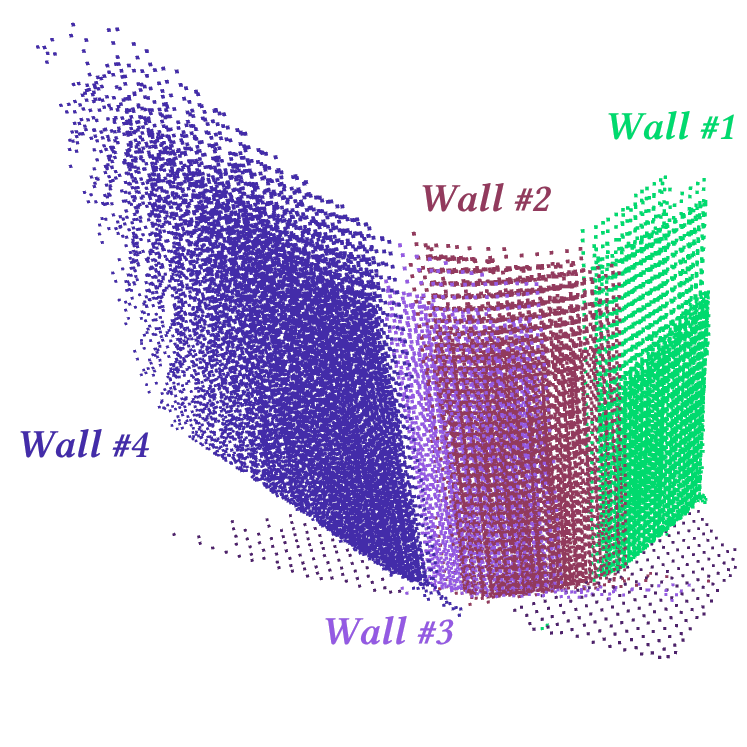
(a) Incorrect planar approximation of a curved wall as multiple flat walls in the ICL dataset [28]

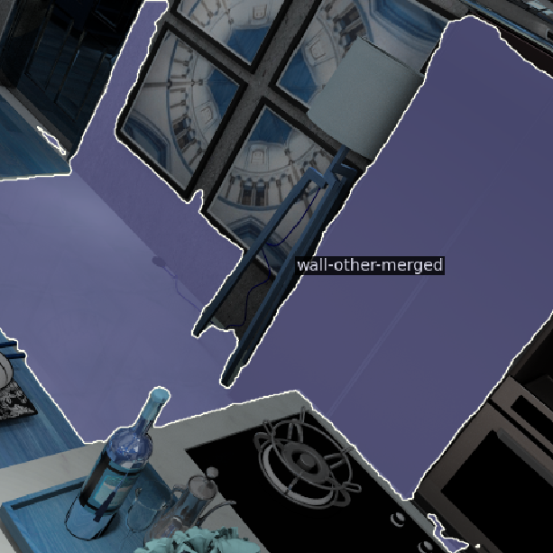
(b) Misclassification and erroneous wall segmentation in the ICL [28] dataset

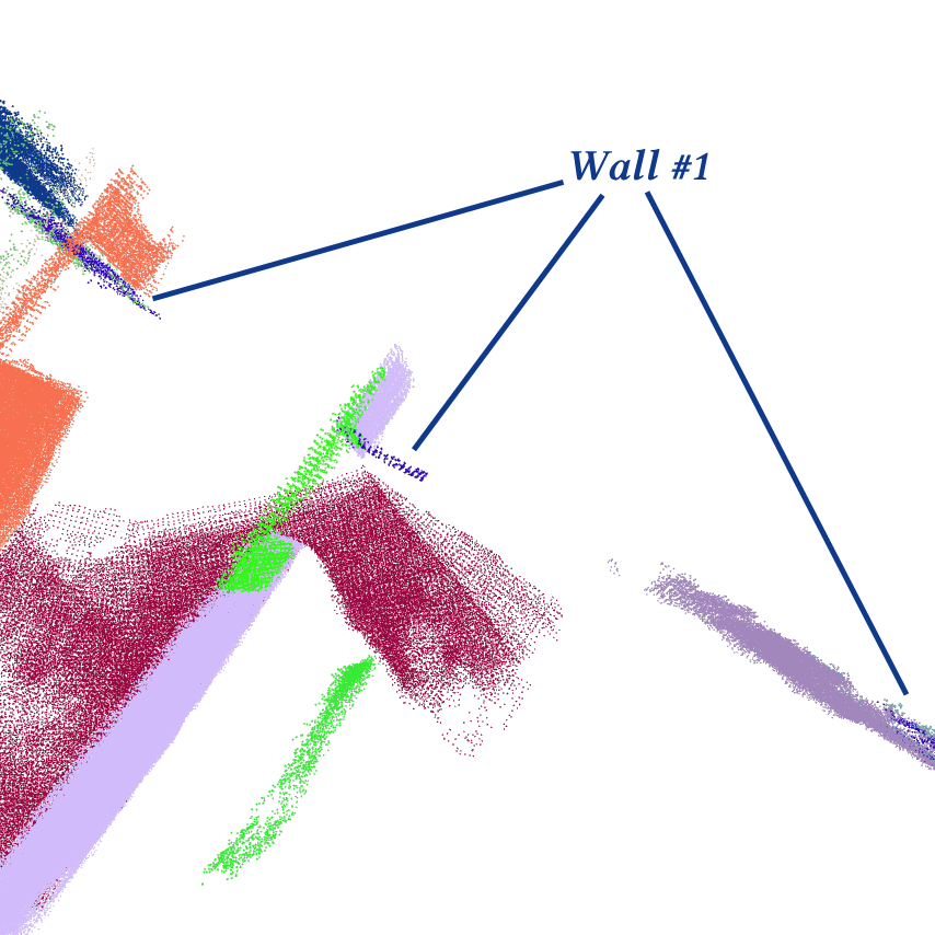
(c) Wrong merging of separate wall segments as one due to weak boundary constraints

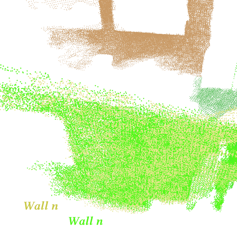
(d) Failure to associate segments of a single wall in the AutoSense dataset

Figure 8: Challenges faced by vS-Graphs, leading to inaccuracies in scene understanding and map reconstruction. Labels have been arbitrarily added for better clarification.

Apart from trajectory estimation improvements and enriched map reconstruction by vS-Graphs, some limitations remain to be studied and addressed. A primary challenge shared by vS-Graphs and its baseline arises in low-texture scenes (e.g., corridors with uniformly painted walls), negatively impacting feature-matching and tracking procedures. In vS-Graphs, this can affect pose estimation and localization of building components and propagate the error through the high-level element recognition stage. Fig. 8 depicts some factors that contribute to lower accuracy w.r.t. the baseline in evaluations. Accordingly, relying on detecting planar surfaces as building components might limit the framework’s applicability in environments with irregular geometries (e.g., curved walls in Fig. 8(a)). Misclassifying semantic entities in the corresponding module (Fig. 8(b)) can also lead to incorrect environment understanding and scene graph generation. Finally, overly/loosely permissive association thresholds essential for building component identification are crucial for robust performance, as shown in Fig. 8(c)-8(d).

6 Conclusions

This paper introduced vS-Graphs, a real-time Visual SLAM (VSLAM) framework that reconstructs the robot’s operating environment using optimizable hierarchical 3D scene graphs. To achieve this, the framework detects building components (i.e., walls and ground surfaces), from which structural elements (i.e., rooms and corridors) are inferred, and incorporates them all into hierarchical representations. As a result, beyond enhancing map reconstruction by integrating these meaningful entities, vS-Graphs offers structured and flexible representations of spatial relationships among high-level environment-driven semantic objects. Experimental results using standard and in-house indoor datasets demonstrated that the proposed framework leads to superior trajectory estimation and mapping performance compared to the baseline and state-of-the-art VSLAM methodologies, reducing trajectory error by up to $9.58\%$ on real-world collected dataset instances. Other evaluations showed that the visual features processed by vS-Graphs enable the identification of semantic entities effectively describing the environment’s layout with accuracy comparable to precise LiDAR-based methods.

Future work includes integrating additional building components (e.g., ceilings, windows, and doorways) and structural elements (e.g., floors) to enrich the reconstructed maps, along with extending support for detecting irregular room layouts (e.g., non-rectangular spaces) and non-linear walls (e.g., curved surfaces). We also plan to release the source code publicly, enabling researchers to further develop and validate the framework.

References

- [1] H. Bavle, J. L. Sanchez-Lopez, C. Cimarelli, A. Tourani, and H. Voos, “From slam to situational awareness: Challenges and survey,” Sensors, vol. 23, no. 10, p. 4849, 2023.
- [2] H. Pu, J. Luo, G. Wang, T. Huang, and H. Liu, “Visual slam integration with semantic segmentation and deep learning: A review,” IEEE Sensors Journal, 2023.
- [3] D. Cai, R. Li, Z. Hu, J. Lu, S. Li, and Y. Zhao, “A comprehensive overview of core modules in visual slam framework,” Neurocomputing, p. 127760, 2024.
- [4] H. Pu, J. Luo, G. Wang, T. Huang, and H. Liu, “Visual slam integration with semantic segmentation and deep learning: A review,” IEEE Sensors Journal, 2023.
- [5] S. Garrido-Jurado, R. Muñoz-Salinas, F. J. Madrid-Cuevas, and M. J. Marín-Jiménez, “Automatic generation and detection of highly reliable fiducial markers under occlusion,” Pattern Recognition, vol. 47, no. 6, pp. 2280–2292, 2014.
- [6] A. Rosinol, A. Gupta, M. Abate, J. Shi, and L. Carlone, “3d dynamic scene graphs: Actionable spatial perception with places, objects, and humans,” 2020.
- [7] S. Koch, P. Hermosilla, N. Vaskevicius, M. Colosi, and T. Ropinski, “Sgrec3d: Self-supervised 3d scene graph learning via object-level scene reconstruction,” in Proceedings of the IEEE/CVF Winter Conference on Applications of Computer Vision, 2024, pp. 3404–3414.
- [8] S.-C. Wu, J. Wald, K. Tateno, N. Navab, and F. Tombari, “Scenegraphfusion: Incremental 3d scene graph prediction from rgb-d sequences,” in Proceedings of the IEEE/CVF Conference on Computer Vision and Pattern Recognition, 2021, pp. 7515–7525.
- [9] H. Bavle, J. L. Sanchez-Lopez, M. Shaheer, J. Civera, and H. Voos, “S-graphs+: Real-time localization and mapping leveraging hierarchical representations,” IEEE Robotics and Automation Letters, vol. 8, no. 8, pp. 4927–4934, 2023.
- [10] N. Hughes, Y. Chang, and L. Carlone, “Hydra: A real-time spatial perception system for 3d scene graph construction and optimization,” 2022.
- [11] C. Campos, R. Elvira, J. J. G. Rodríguez, J. M. Montiel, and J. D. Tardós, “Orb-slam3: An accurate open-source library for visual, visual-inertial, and multimap slam,” IEEE Transactions on Robotics, vol. 37, no. 6, pp. 1874–1890, 2021.
- [12] A. Tourani, H. Bavle, J. L. Sanchez-Lopez, and H. Voos, “Visual slam: What are the current trends and what to expect?” Sensors, vol. 22, no. 23, p. 9297, 2022.
- [13] T. Whelan, S. Leutenegger, R. F. Salas-Moreno, B. Glocker, and A. J. Davison, “Elasticfusion: Dense slam without a pose graph.” in Robotics: science and systems, vol. 11. Rome, Italy, 2015, p. 3.
- [14] T. Schops, T. Sattler, and M. Pollefeys, “Bad slam: Bundle adjusted direct rgb-d slam,” in Proceedings of the IEEE/CVF Conference on Computer Vision and Pattern Recognition, 2019, pp. 134–144.
- [15] C. Yan, D. Qu, D. Xu, B. Zhao, Z. Wang, D. Wang, and X. Li, “Gs-slam: Dense visual slam with 3d gaussian splatting,” in Proceedings of the IEEE/CVF Conference on Computer Vision and Pattern Recognition, 2024, pp. 19 595–19 604.
- [16] Z. Peng, T. Shao, Y. Liu, J. Zhou, Y. Yang, J. Wang, and K. Zhou, “Rtg-slam: Real-time 3d reconstruction at scale using gaussian splatting,” in ACM SIGGRAPH 2024 Conference Papers, 2024, pp. 1–11.
- [17] N. Keetha, J. Karhade, K. M. Jatavallabhula, G. Yang, S. Scherer, D. Ramanan, and J. Luiten, “Splatam: Splat track & map 3d gaussians for dense rgb-d slam,” in Proceedings of the IEEE/CVF Conference on Computer Vision and Pattern Recognition, 2024, pp. 21 357–21 366.
- [18] M. Grinvald, F. Furrer, T. Novkovic, J. J. Chung, C. Cadena, R. Siegwart, and J. Nieto, “Volumetric instance-aware semantic mapping and 3d object discovery,” IEEE Robotics and Automation Letters, vol. 4, no. 3, pp. 3037–3044, 2019.
- [19] Z. Zhu, S. Peng, V. Larsson, W. Xu, H. Bao, Z. Cui, M. R. Oswald, and M. Pollefeys, “Nice-slam: Neural implicit scalable encoding for slam,” in Proceedings of the IEEE/CVF conference on computer vision and pattern recognition, 2022, pp. 12 786–12 796.
- [20] X. Yuan and S. Chen, “Sad-slam: A visual slam based on semantic and depth information,” in 2020 IEEE/RSJ International Conference on Intelligent Robots and Systems (IROS). IEEE, 2020, pp. 4930–4935.
- [21] J. He, M. Li, Y. Wang, and H. Wang, “Ovd-slam: An online visual slam for dynamic environments,” IEEE Sensors Journal, vol. 23, no. 12, pp. 13 210–13 219, 2023.
- [22] P. Cong, J. Liu, J. Li, Y. Xiao, X. Chen, X. Feng, and X. Zhang, “Ydd-slam: Indoor dynamic visual slam fusing yolov5 with depth information,” Sensors, vol. 23, no. 23, p. 9592, 2023.
- [23] J. Han, R. Dong, and J. Kan, “Basl-ad slam: A robust deep-learning feature-based visual slam system with adaptive motion model,” IEEE Transactions on Intelligent Transportation Systems, 2024.
- [24] A. Tourani, H. Bavle, J. L. Sanchez-Lopez, R. M. Salinas, and H. Voos, “Marker-based visual slam leveraging hierarchical representations,” in 2023 IEEE/RSJ International Conference on Intelligent Robots and Systems (IROS), 2023, pp. 3461–3467.
- [25] A. Tourani, H. Bavle, D. I. Avşar, J. L. Sanchez-Lopez, R. Munoz-Salinas, and H. Voos, “Vision-based situational graphs exploiting fiducial markers for the integration of semantic entities,” Robotics, vol. 13, no. 7, p. 106, 2024.
- [26] J. Hu, L. Huang, T. Ren, S. Zhang, R. Ji, and L. Cao, “You only segment once: Towards real-time panoptic segmentation,” in Proceedings of the IEEE/CVF Conference on Computer Vision and Pattern Recognition, 2023, pp. 17 819–17 829.
- [27] K. G. Derpanis, “Overview of the ransac algorithm,” Image Rochester NY, vol. 4, no. 1, pp. 2–3, 2010.
- [28] S. Saeedi, E. D. Carvalho, W. Li, D. Tzoumanikas, S. Leutenegger, P. H. Kelly, and A. J. Davison, “Characterizing visual localization and mapping datasets,” in 2019 International Conference on Robotics and Automation (ICRA). IEEE, 2019, pp. 6699–6705.
- [29] X. Shi, D. Li, P. Zhao, Q. Tian, Y. Tian, Q. Long, C. Zhu, J. Song, F. Qiao, L. Song et al., “Are we ready for service robots? the openloris-scene datasets for lifelong slam,” in 2020 IEEE International Conference on Robotics and Automation (ICRA). IEEE, 2020, pp. 3139–3145.
- [30] A. Dai, A. X. Chang, M. Savva, M. Halber, T. Funkhouser, and M. Nießner, “Scannet: Richly-annotated 3d reconstructions of indoor scenes,” in Proceedings of the IEEE conference on computer vision and pattern recognition, 2017, pp. 5828–5839.
- [31] J. Sturm, N. Engelhard, F. Endres, W. Burgard, and D. Cremers, “A benchmark for the evaluation of rgb-d slam systems,” in 2012 IEEE/RSJ international conference on intelligent robots and systems. IEEE, 2012, pp. 573–580.