Price Impact of Health Insurance

Abstract

This paper examines the equilibrium effects of insurance contracts on healthcare markets using a mechanism design framework. A population of risk-averse agents with preferences as in Yaari (1987) face the risk of developing an illness of unknown severity, which can be treated in a competitive hospital services market at the prevailing market price. After privately observing their health risk, but before learning their sickness level, agents have the option to purchase insurance from a monopolistic provider. Insurance contracts specify premiums, out-of-pocket costs (OPCs), and hospital service coverage, thus determining demand and price in the downstream hospital market through a market-clearing condition. Our first main result shows that optimal insurance contracts take a simple form: agents can choose between full hospital coverage with a high OPC or restricted coverage with a low OPC. This highlights a novel form of under-insurance—rationing or restricted access to healthcare services—emerging purely due to the insurer’s attempt to control his price impact. Our second key result illustrates the nuanced effect of price impact on the amount of insurance provided. Higher healthcare prices increase insurer payouts but also worsen agents’ outside options, making them more willing to pay for insurance ex ante. The net effect of these forces determines whether insurance provision exceeds or falls short of a price-taking benchmark.
Keywords: insurance, mechanism design, market design, healthcare markets
JEL Codes: I11, I13, D47, D81, D82, D86

Preliminary Draft

1 Introduction

Insurance plays a crucial role in mitigating health risks by covering a portion of medical expenses incurred by its customers. While the contract theory literature has extensively studied the optimal design of insurance contracts in the presence of adverse selection and moral hazard, less attention has been devoted to the equilibrium effects of health insurance. The type and level of insurance coverage typically influence the demand for healthcare services, which in turn affects prices, payouts, and the overall cost of insurance provision. Given that large insurance companies are likely to internalize these forces when designing contracts, a key question arises: how does the interaction between insurance and healthcare markets shape both the types of contracts offered and the amount of insurance provided?

This paper addresses these questions by incorporating equilibrium effects into a mechanism design framework. Specifically, we examine the problem faced by a risk-neutral monopolistic insurer serving a population of agents who are risk-averse in the sense of Yaari (1987), and are privately informed of both their probability of developing an illness ex ante, and of the realized illness level ex post. An insurance contract consists of three key components: $(i)$ a premium, $(ii)$ an out-of-pocket expense, and $(iii)$ the amount of hospital services covered. The insurer selects a menu of contracts to maximize profit, subject to individual rationality and (ex-ante and ex-post) incentive compatibility constraints. However, the insurer must also account for the fact that each menu influences demand in the competitive healthcare market, and, through a market-clearing condition—requiring that demand matches available supply— healthcare prices and thus the cost of insurance provision.

Our first main result, Theorem 1, characterizes the equilibrium contracts using tools from optimal transport. Despite the complexity of the setting, we find that optimal contracts take a simple form: they offer at most two options. The first option provides full access to hospital services at a high out-of-pocket cost, while the second restricts access to hospital services in exchange for a lower out-of-pocket cost. This result establishes that rationing—or restricted access to treatment—can emerge in the healthcare market due to the insurer’s attempt to control his price impact. Specifically, after purchasing insurance, some agents may wish to consume more hospital services at the given OPC but are constrained by the limits imposed by the insurer. Importantly, restricted access to hospital services differs from other forms of under-insurance, which typically arise due to information frictions such as moral hazard or adverse selection. In those cases, insurers raise out-of-pocket costs to limit access to insurance, but do not impose caps on healthcare services. While this is a feasible mechanism to control healthcare prices in our model, the insurer instead chooses to curtail demand by restricting access to hospital services directly. In other words, rationing arises only when the insurer internalizes his impact on market prices; absent this effect, no restriction on healthcare services would occur. This result thus provides a rationale for the treatment limitations commonly observed in real-world insurance contracts.

Our second main result, Theorem 2, examines the nuanced effects of price impact on the amount of insurance provided. Higher healthcare prices increase payouts, generating incentives for a profit-maximizing insurer to reduce coverage. At the same time, however, they also raise the demand for insurance, since agents now face larger prices upon getting sick, and thus are exposed to more risk ex ante. Put differently, higher healthcare prices lead to a worse outside option (an endogenous object in our model) for the agents, which increases their willingness to pay for insurance and allows the insurer to charge higher premiums. The prevailing of the two effects determines whether in equilibrium we observe over or under insurance relative to a price-taking benchmark, in which the insurer does not internalize his impact on healthcare prices.

Related literature.

The relationship between health insurance and healthcare prices has been analyzed at least since the seminal work of Feldstein (1970) (see also Feldstein, 1973; Baker et al., 2015). However, to the best of our knowledge, our paper is the first to address the problem within a mechanism design framework. This approach is particularly desirable given our research question, as it imposes minimal restrictions on the types of contracts insurers can offer, allowing us to determine precisely the effect of market forces on the shape of equilibrium insurance contracts. Indeed, one of the main contributions of the paper is precisely to show that rationing of healthcare services can arise in a competitive healthcare market as a result of market power in the insurance market.

This paper contributes to the extensive literature on insurance with adverse selection and moral hazard (see, for instance, Stiglitz, 1977; Grossman and Hart, 1983; Chade and Schlee, 2012). Particularly relevant to our analysis is the recent work by Gershkov et al. (2023), who examine the classical monopoly insurance problem under adverse selection. Their model, however, departs from the canonical framework of Stiglitz (1977) in two key respects.

First, they allow for highly general distributions of losses, which may be correlated with the agent’s private information. Second, agents are assumed to have risk-averse preferences represented by a dual utility functional (Yaari, 1987). Unlike the expected utility framework, dual utility incorporates a non-linear transformation of probabilities rather than payoffs. As demonstrated by Yaari (1987), this representation arises from a single modification to expected utility theory: instead of requiring independence with respect to probability mixtures of risky lotteries, it requires independence concerning direct mixtures of payments associated with risky lotteries.

Gershkov et al. (2023) argue that dual utility is a particularly compelling framework for several reasons. First, empirical studies (Sydnor, 2010; Barseghyan et al., 2013, 2016) document insurance choice patterns that are difficult to reconcile with expected utility but align well with models involving probability weighting—a feature inherent in dual utility. Second, dual utility maintains linearity in wealth, meaning it captures risk aversion while preserving constant marginal utility of wealth. This property enhances the tractability of their model relative to traditional approaches. Consequently, Gershkov et al. (2023) are able to explain real-world contract features that standard expected utility frameworks struggle to rationalize. Notably, they identify conditions under which insurers optimally offer deductible and coverage limit contracts.

Motivated by these insights, we also endow agents with Yaari-risk preferences, but consider a fundamentally different model, in which the risk-averse agent is exposed to a loss (sickness) which can only be cured by a hospital. This implicitly generates costs of insurance provision: the only way to shield the agent from risk—and thus extract surplus— is to encourage her to visit the hospital more often, which in turn increases the probability that the insurer has to cover (a fraction of) the market price. Moreover, since in our model the outside option of the agents is to visit the hospital without insurance, and thus pay the full market price, the insurer’s choice of mechanism directly influences the value of this outside option through its effect on the market price.

Our second departure from the previous literature on insurance is that the price of hospital services (and hence the cost of insurance provision) is endogenously determined by the demand for healthcare induced by the insurer and available supply. We thus contribute to the growing literature examining the equilibrium effects of mechanisms, arising when the designer does not control the entire market (Tirole, 2012; Dworczak et al., 2021; Loertscher and Muir, 2022; Kang, 2023). Consistently with this literature, we find that rationing can arise as an equilibrium outcome. In our case, the insurer’s attempt to control her price impact determines rationing in the market of hospital services. Compared to previous papers, we encounter an additional technical difficulty due to the fact that our principal has to account for the price impact while facing a sequential screening problem reminiscent of the one analyzed in Courty and Hao (2000), and mechanisms take the form of “menus of menus”. We tackle this by using results from optimal transport to generalize the techniques recently exploited by Dworczak et al. (2021) and Kang (2023) to a multi-dimensional setting.

The rest of the paper proceeds as follows. In Section 2 we go over the model. In Section 3 we characterize the optimal insurance menu, for a given price of healthcare services. In Section 4 we allows the insurer to also pick the preferred price of hospital services, and provide a condition to determine whether we have over or under-insurance relative to a price-taking benchmark. Section 5 concludes.

2 Model

Distribution of Disease Levels.

A unit mass of agents face the risk of developing an illness with severity $b\in\left[0,\bar{b}\right)\equiv B$, distributed according to the cumulative distribution function $H_{\theta}:B\to[0,1]$, where the maximum level $\bar{b}$ may be finite or infinite. An agent (she) privately observes her realized disease level $b$, which also represents the monetary amount she is willing to pay to eliminate the illness. A higher $b$ indicates a more severe condition and, consequently, a greater willingness to pay for its resolution.

In addition to $b$, the agent’s private information includes her risk type $\theta\in\left[\underline{\theta},\bar{\theta}\right]\equiv\Theta$, which parametrizes her distribution of disease levels $H_{\theta}$. We assume that $H_{\theta}$ increases in $\theta$ in the sense of first-order stochastic dominance, meaning that higher risk types face stochastically larger disease levels. We denote by $F:\Theta\rightarrow[0,1]$ the distribution of risk types and by $f:\Theta\rightarrow(0,\infty)$ its density. Additionally, we impose the following technical assumptions: $H_{\theta}$ is continuously differentiable in $\theta$, and for each fixed $\theta$, the function $H_{\theta}(\cdot)$ is differentiable on $B$ with derivative $h_{\theta}:B\rightarrow(0,\infty)$.

Example 1

Risk type $\theta$ represents the probability of suffering an illness. Conditional on suffering the illness, its severity level is uniformly distributed on $[0,1]$. Then, $H_{\theta}$ is given by:

$$H_{\theta}(b)=1-\theta+\theta b.$$

Hospital Services.

After drawing a disease level $b$, an agent can visit the hospital and get cured for a price $p\in\mathbb{R}_{+}$. We assume that agents do not face budget constraints. Since $b$ represents the agent’s willingness to pay to eliminate the illness, she will visit the hospital whenever $b>p$. In this case, the loss becomes $p$ instead of $b$.

Additionally, we allow for the possibility of partial treatment or non-unit demand for hospital services, modeled as the ability of the agent to have any fraction $x\in[0,1]$ of the illness cured for a total expense of $xp$. An agent with sickness level $b$ who decides to purchase $x$ units of hospital services faces an effective loss of $(1-x)b+xp$.

The ability to access fractional amounts of hospital services will become crucial once we analyze the insurer’s problem, however, without insurance, it is clearly inconsequential. Indeed, if $b\leq p$, curing any positive fraction of the illness yields a loss of $(1-x)b+xp\geq b$, so the agent is always weakly better off choosing $x=0$. Conversely, if $b>p$, curing any fraction less than 1 results in a loss of $(1-x)b+xp<b$, so the agent strictly prefers to set $x=1$.

Thus, the provision of hospital services at a price $p$, in the absence of insurance, modifies risk type $\theta$’s distribution of disease levels to:

$$H^{p}_{\theta}(b)=\begin{cases}H_{\theta}(b)&\text{if }b<p,\\ 1&\text{if }b\geq p.\end{cases}$$

Finally, we assume that the market for hospital services is competitive and characterized by a strictly increasing supply function, denoted by $S:\mathbb{R}_{+}\to\mathbb{R}_{+}$, where $S(p)$ represents the quantity of hospital services supplied at price $p$. Additionally, we impose the following technical assumptions: $S$ is differentiable, unbounded and satisfies $S(0)=0$.

The Agent’s Utility Function.

As in Gershkov et al. (2023), agents are endowed with a Yaari (dual) utility determined by a probability distortion function $g:[0,1]\to[0,1]$, where $g$ is increasing, continuously differentiable, and satisfies $g(q)\leq q$ with $g(0)=0$ and $g(1)=1$.

The certainty equivalent of suffering a random loss distributed according to $H_{\theta}$ is given by:

$$CE(H_{\theta}(b))=-\int_{0}^{\bar{b}}[1-g(H_{\theta}(b))]\,db.$$

In particular, if hospital services are provided at a price $p$, such that the effective distribution of disease levels becomes $H^{p}_{\theta}$, the certainty equivalent becomes:

$$CE\left(H^{p}_{\theta}(b)\right)=-\int_{0}^{p}[1-g(H_{\theta}(b))]\,db,$$

where we use the fact that $H^{p}_{\theta}(b)=H_{\theta}(b)$ for all $b<p$, $H^{p}_{\theta}(b)=1$ for all $b\geq p$, and $g(1)=1$.

As discussed in Gershkov et al. (2023), the agent is risk-averse in the weak sense: the certainty equivalent of any lottery is less than the lottery’s expected value. That is:

$$CE(H_{\theta}(b))=-\int_{0}^{\bar{b}}[1-g(H_{\theta}(b))]\,db\leq-\int_{0}^{\bar{b}}[1-H_{\theta}(b)]\,db=-\mathbb{E}_{H_{\theta}}[b],$$

where the inequality follows from $g(q)\leq q$, and $\mathbb{E}_{H_{\theta}}[b]$ represents the expected value of $b$ under $H_{\theta}$.

While in the expected utility framework, this form of risk aversion is equivalent to aversion to mean-preserving spreads, in the dual utility framework, aversion to mean-preserving spreads is stronger and is equivalent to $g$ being convex. As in Gershkov et al. (2023), the weak form of risk aversion, which requires only $g(q)\leq q$, is sufficient for our analysis.

To better understand dual utility, we can use integration by parts to express the certainty equivalent of the lottery $H_{\theta}$ as:

$$CE(H_{\theta}(b))=-\int_{0}^{\bar{b}}[1-g(H_{\theta}(b))]\,db=-\int_{0}^{\bar{b}}bg^{\prime}(H_{\theta}(b))\,db$$

In contrast to the expected utility framework—where the standard expectation operator is modified by distorting payoffs through the von Neumann–Morgenstern utility function—dual utility modifies the expected value of the lottery by distorting probabilities through $g^{\prime}$. Here, every loss $b$ is weighted by $g^{\prime}(H_{\theta}(b))$. The term $g(H_{\theta}(b))$ represents the cumulative weight assigned to losses below $b$, while $1-g(H_{\theta}(b))$ represents the cumulative weight assigned to losses above $b$. The assumption $g(q)\leq q$ implies that the agent overweights the cumulative probability of larger losses and underweights the cumulative probability of smaller losses.

Figure 1 illustrates the certainty equivalent of a risk-neutral agent and a risk-averse agent endowed with a Yaari utility determined by $g(q)=q^{2}$, when both face the lottery $H^{p}_{\theta}$, and the distribution $H_{\theta}$ is as in Example 1. The blue curve represents the distribution $H_{\theta}^{p}(b)$, and the red curve $g(H_{\theta}^{p}(b))$. The area above the blue curve denotes the expected value of $H^{p}_{\theta}$, which is also the certainty equivalent of the risk-neutral agent. The area above the red curve and below the horizontal dashed line represents the certainty equivalent of the risk-averse agent. The area between the red and blue curves represents the additional money the risk-averse agent is willing to pay to eliminate the risk of lottery $H^{p}_{\theta}$.

Figure 1: $H_{\theta}(b)=1-\theta+\theta b$,  $\theta=0.7$,  $g(q)=q^{2}$

Finally, another key property of Yaari utility is its additivity with respect to constant random variables $t$:

$$CE(H_{\theta}+t)=CE(H_{\theta})+t.$$

As noted by Yaari (1987), in the expected utility framework, the agent’s attitude toward risk and their attitude toward wealth are inherently linked. Specifically, a risk-averse agent will always exhibit decreasing marginal utility with respect to wealth. In contrast, under dual utility, an agent can maintain constant marginal utility over wealth while still displaying risk aversion toward uncertain outcomes. The separability of preferences with respect to constant random variables, combined with the fact that Yaari utility distorts probabilities rather than payoffs, provides crucial tractability for our analysis.

Insurance.

A risk-neutral monopolistic insurance provider (he) offers a mechanism to the agents. The mechanism is offered when an agent knows only her risk type $\theta$ before $b$ has been realized. We assume that the provider can contract with agents on the following: 1) the amount of treatment or quantity of hospital services, $x$, that an agent can access with insurance; 2) the portion of the price $p$ of hospital services that an agent will cover when using insurance, referred to as the out-of-pocket cost (OPC), denoted by $C$; and 3) an upfront payment or premium, $t$, that an agent must pay to access her insurance.

Additionally, we restrict our attention to: 1) direct mechanisms and 2) non-randomized mechanisms. Focusing on direct mechanisms is without loss of generality, as the revelation principle applies in our setting. While Gershkov et al. (2023) also study non-randomized mechanisms, they note that this restriction is not without loss: lotteries over insurance contracts could help the provider better screen risk-averse agents. However, focusing on non-randomized mechanisms is appropriate for insurance applications, as lotteries over contracts are rarely observed in practice.

More formally, a mechanism (or menu) is represented as:

$$\left\{\left(\left\{\left(x(\theta,b),C(\theta,b)\right)\right\}_{b\in B},t(\theta)\right)\right\}_{\theta\in\Theta},$$

where each menu option includes a contract $\left\{\left(x(\theta,b),C(\theta,b)\right)\right\}_{b\in B}$ and a premium $t(\theta)\in\mathbb{R}$. Upon visiting the hospital, an agent with the contract $\left\{\left(x(\theta,b),C(\theta,b)\right)\right\}_{b\in B}$ can choose any of its items. If the agent selects the item $\left(x(\theta,b),C(\theta,b)\right)$, she can access up to $x(\theta,b)\in[0,1]$ units of hospital services for an OPC of $C(\theta,b)\in\mathbb{R}_{+}$, with the insurer covering the remaining cost.

Figure 2 illustrates the timing of the interaction between the insurer and the agents, which we describe more precisely as follows:

1. The insurer commits to and offers the agents a menu:

   $$\left\{\left(\left\{\left(x(\theta,b),C(\theta,b)\right)\right\}_{b\in B},t(\theta)\right)\right\}_{\theta\in\Theta}.$$

2. The agents privately observe their risk type $\theta$, decide whether to participate in the mechanism and, if so, they select an option from the menu, and pay the corresponding premium.

3. The sickness level $b$ is realized and privately observed by the agents. An agent holding the contract $\left\{\left(x(\theta,b),C(\theta,b)\right)\right\}_{b\in B}$ decides whether to visit the hospital or remain at home. If the agent visits the hospital, they may demand any quantity of hospital services. Payment can be made entirely out of pocket or by selecting a contract item. If the agent chooses the item $\left(x(\theta,b),C(\theta,b)\right)$, they are entitled to up to $x(\theta,b)$ units of hospital services at an out-of-pocket cost of $C(\theta,b)$. However, for any additional units exceeding $x(\theta,b)$, the agent must pay the full hospital price.

4. The contracts chosen by the agents, along with the items selected from the contracts, generate a demand for hospital services at a given price. The market for hospital services clears at the price where demand equals supply, and payoffs are accrued.

Figure 2: Timeline

The objective of the insurer is to find a menu that maximizes his profits. However, since a menu influences the equilibrium hospital price, which in turn affects both the agents’ behavior and the insurer’s profits, we adopt a two-stage approach to determine the optimal menu: 1) In the first stage, we fix a price for hospital services, $p$, and identify, among the menus that sustain that price in equilibrium, the one that maximizes the insurer’s profits. 2) Once the first stage is complete, we associate each achievable price in equilibrium with the corresponding profits obtained by the insurer, and then solve for the price that maximizes these profits.

3 First Stage: Optimal Insurance Menus

In this section, we fix and denote by $p\in\mathbb{R}_{+}$ the price for hospital services. Our goal is to identify the set of implementable menus that sustain $p$ in equilibrium. Once this step is completed, we will be able to formally define and solve the insurer’s first-stage problem.

3.1 Implementable Menus

Period 2 Incentive Compatibility.

After an agent with risk type $\theta^{\prime}$ selects an option from the menu and her disease level $b$ is realized, she makes a series of decisions. First, she chooses whether to visit the hospital or remain at home. If she decides to visit the hospital, she has two payment options: covering the medical bill entirely out of pocket or utilizing an item from her contract $\left\{\left(x(\theta,b),C(\theta,b)\right)\right\}_{b\in B}$. The agent’s loss function when engaging with the item $\left(x(\theta,b^{\prime}),C(\theta,b^{\prime})\right)$ is defined as follows:

$$L(b,b^{\prime};\theta)=x(\theta,b^{\prime})\min\{C(\theta,b^{\prime}),b_{p}\}+(1-x(\theta,b^{\prime}))b_{p},$$

where $b_{p}=\min\{b,p\}$.

We now explain why this expression represents the agent’s loss. The agent will visit the hospital and utilize the maximum amount of hospital services covered by the contract item, $x(\theta,b)$, if the out-of-pocket cost $C(\theta,b^{\prime})$ is less than $b_{p}$. In this case, the treatment cost is $x(\theta,b)C(\theta,b^{\prime})$.

If $b$ is higher than $p$, the agent will also demand the remaining portion of hospital services, $1-x(\theta,b)$, at the full hospital price $p$. The additional treatment cost is $(1-x(\theta,b))p$, resulting in a total loss of $x(\theta,b)C(\theta,b^{\prime})+(1-x(\theta,b))p$.

However, if $b$ is lower than $p$, the agent will not demand the remaining portion, and her loss will instead be $x(\theta,b)C(\theta,b^{\prime})+(1-x(\theta,b))b$.

Conversely, if $C(\theta,b^{\prime})$ is higher than $b_{p}$, two scenarios may arise: 1) If the hospital price $p$ is lower than both her disease level $b$ and $C(\theta,b^{\prime})$, it becomes more cost-effective for the agent to utilize the full unit of hospital services and pay the entire treatment cost out of pocket. In this situation, her loss is $p$. 2) If her disease level $b$ is lower than both $p$ and $C(\theta,b^{\prime})$, the agent prefers to remain at home, and her loss is $b$.

It is important to note that the agent’s risk type $\theta^{\prime}$ is irrelevant in determining her loss function. At this stage, the only relevant variables are her actual disease level $b$, the contract chosen from the menu (indexed by $\theta$), and the item selected from the contract (indexed by $b^{\prime}$). Figure 3 illustrates the agent’s behavior and her resulting loss when she selects the item from the contract corresponding to her true disease level.

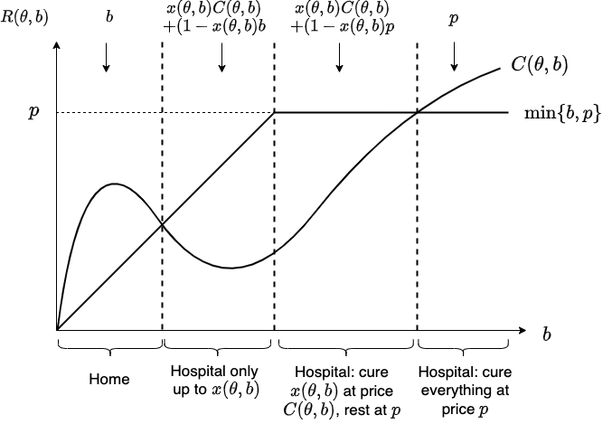
Figure 3: Loss and behavior of an agent that truthfully reports her disease level.

Having introduced the agent’s period 2 loss function, we can now define the usual incentive compatibility constraint that a contract must satisfy. Specifically, it suffices to focus on contracts where the agent truthfully reports her disease level:

$$L(b;\theta)\equiv L(b,b;\theta)\leq L(b,b^{\prime};\theta)\;\;\text{for all $b,b^{\prime}\in B$.} IC_{2}$$ ()

We now show some properties of contracts that satisfy $IC_{2}$:

Lemma 1

Without loss of generality we can restrict attention to contracts that satisfy $C(\theta,b)\leq b_{p}$.

Lemma 2

A contract satisfies $IC_{2}$ only if $L(p;\theta)=L(b;\theta)$ for all $b>p$. Furthermore, without loss of generality, we can restrict attention to contracts that satisfy $x(\theta,b)=1$ for all $b>p$.

The formal proofs of Lemmas 1 and 2 can be found in Appendix B.

Lemmas 1 and 2 are intuitive. For Lemma 1, if $C(\theta,b)>b_{p}$, the agent will not use her insurance. The insurer can replicate this outcome by setting $C(\theta,b)\leq b_{p}$ but restricting the agent’s access to hospital services by setting $x(\theta,b)=0$.

For Lemma 2, note that all agents with $b\geq p$ incur the same loss from any allocation. These are the agents who would always go to the hospital in the absence of insurance, effectively behaving as if they have the same disease level or period 2 type. To satisfy $IC_{2}$, all such agents must experience the same loss.

Moreover, whatever loss they incur can be replicated by an allocation where $x(\theta,b)=1$, without changing the demand for hospital services. This is because these agents would already demand the remaining portion of hospital services, $1-x(\theta,b)$.

Lemmas 1 and 2 allow us to express the loss of an agent with $b\in[0,p]$ when truthfully reporting as:

$$L(b;\theta)=x(\theta,b)C(\theta,b)+(1-x(\theta,b))b.$$

This loss function is linear in $b$ and separable in the out-of-pocket cost. Using standard arguments from mechanism design, we can characterize contracts that satisfy $IC_{2}$ by applying the envelope formula and the monotonicity of $x(\theta,\cdot)$:

Lemma 3

A contract satisfies $IC_{2}$ if and only if:

1. $L(b;\theta)=\int_{0}^{b}(1-x(\theta,l))\,dl$ for all $b\in[0,p]$, and $L(b;\theta)=L(p;\theta)$ for all $b>p$.

2. $x(\theta,\cdot):B\to[0,1]$ is a non-decreasing function, with $x(\theta,b)=1$ for all $b>p$.

The formal proof of Lemma 3 can be found in Appendix B.

Period 1 Incentive Compatibility and Individual Rationality.

By Lemma 3, we know that if an agent with risk type $\theta$ selects the menu option

$$\left(\left\{\left(x(\theta^{\prime},b),C(\theta^{\prime},b)\right)\right\}_{b\in B},t(\theta^{\prime})\right),$$

the agent’s loss function is given by:

$$L(b;\theta^{\prime})=\int_{0}^{b}(1-x(\theta^{\prime},l))\,dl.$$

Observe that $L(\cdot;\theta^{\prime})$ is non-decreasing. Consequently, the lottery faced by risk type $\theta$ in period 1 is represented by $H_{\theta}(L^{-1}(l;\theta^{\prime}))$, where $L^{-1}(l;\theta)=\sup\{z:L(z;\theta)\leq l\}$.

The certainty equivalent that risk type $\theta$ gets from her menu option is given by:

$$U(\theta,\theta^{\prime}) =-t(\theta^{\prime})-\int_{0}^{L(\bar{b};\theta^{\prime})}\left[1-g\left(H_{\theta}\left(L^{-1}(l;\theta^{\prime})\right)\right)\right]\,dl$$

$$=-t(\theta^{\prime})-\int_{0}^{\bar{b}}\frac{\partial L(b;\theta^{\prime})}{\partial b}[1-g(H_{\theta}(b))]\,db$$

$$=-t(\theta^{\prime})-\int_{0}^{p}(1-x(\theta^{\prime},b))[1-g(H_{\theta}(b))]db.$$

The additivity of the premium arises from the fact that dual utility is additive in constant random variables. The second equality follows from the change of variable $b=L^{-1}(l;\theta)$, while the third equality results from $\frac{\partial L(b;\theta^{\prime})}{\partial b}=1-x(\theta^{\prime},b)$ (Lemma 3, Condition (1)), along with the condition $x(\theta^{\prime},b)=1$ for $b>p$ (Lemma 3, Condition (2)).

The certainty equivalent is linear in $x$, a property that provides crucial tractability for the analysis. This linearity arises from Lemma 3 and the fact that dual utility distorts probabilities rather than payoffs.

The period 1 incentive compatibility and individual rationality constraints are as follows:

$$U(\theta)\equiv U(\theta,\theta)\geq U(\theta,\theta^{\prime})\;\;\text{for all $\theta,\theta^{\prime}\in\Theta$,}$$

$$U(\theta)\geq-\int_{0}^{p}[1-g(H_{\theta}(b))]\,db\;\;\text{for all $\theta\in\Theta$.}$$

The agent’s outside option, represented by the right-hand side of the 3.1 constraint, is derived from the assumption that in the absence of insurance and when hospital services are offered at price $p$, the lottery faced by the agent in period 1 is $H^{p}_{\theta}$.

Lemma 4 provides a partial characterization of menus that satisfy 3.1:

Lemma 4

1. A menu satisfies 3.1 only if

   $$U(\theta)=U(\underline{\theta})+\int_{\underline{\theta}}^{\theta}\int_{0}^{p}(1-x(s,b))g^{\prime}(H_{s}(b))\frac{\partial H_{s}(b)}{\partial s}\,db\,ds.$$

2. If a menu satisfies the above condition and $x(\cdot,b):\Theta\to[0,1]$ is a non-decreasing function for all $b\in B$, then the menu satisfies 3.1.

The formal proof of Lemma 4 is in Appendix B.

Condition (1) of Lemma 4 is the standard envelope formula. Importantly, the additivity of dual utility in constant random variables, combined with Condition (1), enables us to determine premiums (up to a constant) as a function of $x$. Additionally, the monotonicity of $x(\cdot,b)$ for all $b$, together with Condition (1), ensures that a menu satisfies 3.1.

However, a menu that satisfies Condition (1) does not necessarily require $x(\cdot,b)$ to be monotonic for all $b$. This result is common in screening environments, where the allocation chosen by the designer for a fixed agent type is infinite- or multi-dimensional (see, for instance, Gershkov et al., 2023 or Courty and Hao, 2000). Nevertheless, monotonicity remains a robust condition, as it does not depend on the functional forms of $g$ or $H_{\theta}$.

Finally, an incentive-compatible menu satisfies 3.1 if and only if it holds for the lowest type:

Lemma 5

Suppose a menu satisfies 3.1. Then, the 3.1 condition is satisfied for all types if and only if it is satisfied for the lowest type, $\underline{\theta}$.

The formal proof of Lemma 5 is in Appendix B.

Lemma 5 follows from the fact that both the agent’s outside option and utility from participation, $U$, are decreasing in $\theta$. However, $U$ decreases more slowly, as $1-x(\theta,b)\in[0,1]$.

Period 3 Equilibrium Constraint.

If each contract in a menu satisfies $IC_{2}$ and the menu satisfies 3.1 and 3.1, the demand for hospital services by an agent with risk type $\theta$ and disease level $b$ is $x(\theta,b)$. This follows because the menu and its contracts are both incentive compatible and individually rational, ensuring that the agent selects the contract item $\left(x(\theta,b),C(\theta,b)\right)$.

Moreover, if $b\leq p$, the agent will not demand any additional units of hospital services, and her demand is fully determined by $x(\theta,b)$. Conversely, if $b>p$, she would, in principle, demand the remaining portion, $1-x(\theta,b)$. However, by Lemma 2, $x(\theta,b)=1$, meaning the remaining portion is zero. Thus, her demand is again fully determined by $x(\theta,b)$.

The demand for hospital services at price $p$ is given by:

$$D(p;x) =\int_{\underline{\theta}}^{\bar{\theta}}\int_{0}^{\bar{b}}x(\theta,b)h_{\theta}(b)\,dbf(\theta)\,d\theta$$

$$=\int_{\underline{\theta}}^{\bar{\theta}}\int_{0}^{p}x(\theta,b)h_{\theta}(b)\,dbf(\theta)\,d\theta+\int_{\underline{\theta}}^{\bar{\theta}}[1-H_{\theta}(p)]f(\theta)\,d\theta,$$

where the second equality follows from the fact that $x(\theta,b)=1$ for all $b>p$.

It is convenient to define the residual supply of hospital services faced by the insurer at price $p$ as:

$$RS(p)=S(p)-\int_{\underline{\theta}}^{\bar{\theta}}[1-H_{\theta}(p)]f(\theta)\,d\theta,$$

where the second term reflects the portion of demand that the insurer cannot influence, as no matter what menu the insurer offers, he cannot affect the demand arising from disease levels higher than $p$.

The equilibrium constraint can then be expressed as:

$$\int_{\underline{\theta}}^{\bar{\theta}}\int_{0}^{p}x(\theta,b)h_{\theta}(b)\,dbf(\theta)\,d\theta=RS(p).$$

The lowest demand that the insurer can generate occurs with a menu that sets $\underline{x}(\theta,b)=0$ for all $\theta$ and $b\in[0,p]$. In this case, the insurer provides no insurance to any agents, and demand is given by:

$$D(p;\underline{x})=\int_{\underline{\theta}}^{\bar{\theta}}[1-H_{\theta}(p)]f(\theta)\,d\theta.$$

Moreover, by our technical assumptions on the supply function $S$ and the distributions of disease levels $H_{\theta}$, there exists a unique strictly positive price $p^{N}$ that satisfies $D\left(p^{N};\underline{x}\right)=S\left(p^{N}\right)$. That is, $p^{N}$ is the price that clears the healthcare services market in the absence of insurance.

Similarly, the highest demand that the insurer can generate occurs with a menu that sets $\overline{x}(\theta,b)=1$ for all $\theta$ and $b\in[0,p]$. In this case, the insurer provides full insurance—or full access to hospital services at zero OPC. Demand in this case is $D\left(p,\overline{x}\right)=1$. Once again, by our technical assumptions, there exists a unique positive price $p^{F}$ such that $D\left(p^{F},\overline{x}\right)=S\left(p^{F}\right)=1$, and $p^{F}>p^{N}$.

We then have the following result:

Lemma 6

There exists a function $x$ that satisfies Condition (2) of Lemma 3, and 3.1 if and only if $p\in\left[p^{N},p^{F}\right]$.

The formal proof of Lemma 6 is provided in Appendix B.

From now on, we assume that $p$ belongs to $\left[p^{N},p^{F}\right]$, ensuring that there exists a feasible menu that induces it as an equilibrium price in the hospital services market.

3.2 Insurer’s Problem

We are now ready to formulate the first-stage insurer’s problem. To do so, the following Lemma provides an expression for the insurer’s objective:

Lemma 7

Suppose that each contract in a menu satisfies $IC_{2}$, and the menu satisfies 3.1 and 3.1. Then, the insurer’s profits from the menu are:

$$\int_{\underline{\theta}}^{\bar{\theta}}\int_{0}^{p}x(\theta,b)J(\theta,b)h_{\theta}(b)\,dbf(\theta)\,d\theta-U(\underline{\theta})-\int_{0}^{p}[1-g(H_{\underline{\theta}}(b))]\,db,$$

where

$$J(\theta,b)=\underbrace{\left[1-g(H_{{\theta}}(b))+\frac{1-F(\theta)}{f(\theta)}g^{\prime}(H_{\theta}(b))\frac{\partial H_{\theta}(b)}{\partial\theta}\right]}_{\text{Period 1 Virtual Value}}\frac{1}{h_{\theta}(b)}+\underbrace{b-p-\frac{1-H_{\theta}(b)}{h_{\theta}(b)}}_{\text{Period 2 Virtual Value}}.$$

The formal proof of Lemma 7 is in Appendix C.

The insurer’s cost of providing any contract is derived from the fact that the portion of the treatment bill paid by the insurer, when facing an agent with risk type $\theta$ and disease level $b$, is $x(\theta,b)(p-C(\theta,b))$. Using the identity $x(\theta,b)C(\theta,b)=L(b;\theta)-(1-x(\theta,b))b$ and the expression for $L(b;\theta)$ obtained in Lemma 3, Condition (1), along with integration by parts, allows us to determine the insurer’s cost.

Once we have an expression for the insurer’s cost, the only remaining step to determine profits is to find an expression for the revenue the insurer receives from premiums. To obtain this, we can apply standard techniques. Specifically, as mentioned earlier, since Yaari utility is additive in constant random variables, $t$ can be expressed as a function of $x$, up to a constant $U(\underline{\theta})$.

To interpret the insurer’s profits, recall that in screening environments with quasi-linear preferences, where a designer allocates an object or good, the classical agent’s virtual value is a key concept in determining whether it is profitable to assign the good to the agent. It is defined as the marginal value from an increase in the allocation minus the information rents. Information rents, in turn, are captured by the inverse hazard rate multiplied by the derivative of the agent’s marginal value with respect to her type.

In period 1, the agent’s private information, or risk type, is denoted by $\theta$, and her utility from an allocation, $x$, is given by $U(\theta)$. Based on this utility, we see that the agent values an additional unit of hospital services (if her future disease level is $b$) by $1-g(H_{\theta}(b))$. This valuation forms the first term in $J(\theta,b)$, referred to as the period 1 virtual value. The derivative of this marginal valuation with respect to the agent’s risk type is given by:

$$-g^{\prime}(H_{\theta}(b))\frac{\partial H_{\theta}(b)}{\partial b}.$$

This term is then multiplied by the inverse hazard rate of the distribution $F$.

In period 2, the agent’s private information shifts to her disease level, denoted by $b$, and her payoff from an allocation is determined by the loss function $L(b;\theta)$. Here, the second term in $J(\theta,b)$, denoted as the period 2 virtual value, is also analogous to the classical virtual value in screening problems but accounts for provision costs. Specifically, the agent’s marginal valuation for an additional unit of hospital services corresponds to her disease level $b$. On the other hand, the insurer’s marginal cost for providing this additional unit is $p$.

The (relaxed) first-stage insurer’s problem is given by:

$$\Pi(p)\equiv \max_{x}\quad\int_{\underline{\theta}}^{\bar{\theta}}\int_{0}^{p}x(\theta,b)J(\theta,b)h_{\theta}(b)\,dbf(\theta)\,d\theta P$$ ()

$$\text{s.t.}\quad\int_{\underline{\theta}}^{\bar{\theta}}\int_{0}^{p}x(\theta,b)h_{\theta}(b)\,dbf(\theta)\,d{\theta}=RS(p), EQ$$ ()

$$\;\;\;\;\;\;\;\;x(\theta,\cdot):B\rightarrow[0,1]\;\text{is non-decreasing for all }\theta. MON$$ ()

In the formulation of $P$, we have already used the fact that, in an optimal menu, the insurer will always set the utility of the lowest risk type equal to her outside option. We refer to $P$ as a relaxed version of the first-stage insurer’s problem because it incorporates all necessary conditions that an implementable menu must satisfy. However, a solution to $P$ is not necessarily implementable. Specifically, it is possible that $x$ does not satisfy 3.1.

The approach, therefore, is to solve $P$ and identify conditions under which the solution is implementable. For instance, by Lemma 4, Condition (2), we know that if the solution satisfies the property that $x(\cdot,b)$ is non-decreasing for all $b$, then $x$ is implementable.

The function $\Pi:\left[p^{N},p^{F}\right]\rightarrow\mathbb{R}$ captures the profits obtained by the insurer from the optimal menu that sustains $p$ in equilibrium.

3.3 Analysis and Results

We begin by stating the main result of the first-stage analysis. This result characterizes the structure of the optimal contracts induced by the $x^{*}$ that solves $P$:

Theorem 1

There exists an $x^{*}$ that solves $P$ such that the contract offered to risk type $\theta$ takes one of the following forms $\{(1,C(\theta))\}$ with $C(\theta)\in[0,p]$, or $\{(\alpha,C_{l}(\theta)),(1,C_{h}(\theta))\}$ where $0\leq C_{l}(\theta)<C_{h}(\theta)\leq p$ and $\alpha\in(0,1)$.

As formalized in Theorem 1, the optimal contract for each risk type has a simple and intuitive structure. The first form of contract is what we refer to as a simple contract or posted OPC contract, as the agent gets a single option—full access to hospital services for an OPC equal to $C(\theta)$. All agents with a disease level higher than $C(\theta)$ take this option. Therefore, they get full treatment for a medical bill of $C(\theta)$.

The second form of contract gives the agent two options. The first option provides full access to hospital services at a high OPC, denoted by $C_{h}(\theta)$. The second option restricts access to hospital services—up to $\alpha$ units—in exchange for a lower OPC, denoted by $C_{l}(\theta)$.

Whenever the contract for risk type $\theta$ contains two options, $\{(\alpha,C_{l}(\theta)),(1,C_{h}(\theta))\}$, it follows that $x^{*}(\theta,\cdot)$ has two jumps, as represented in Figure 4: It is equal to $0$ for values of $b$ less than or equal to $C_{l}(\theta)$ (these are the disease levels that will stay at home), equal to $\alpha$ for values of $b$ in the range $\left(C_{l}(\theta),\frac{C_{h}(\theta)-\alpha C_{l}(\theta)}{1-\alpha}\right]$ (these are the disease levels that will go to the hospital and use the low OPC with partial treatment), and equal to $1$ for values of $b$ greater than $\frac{C_{h}(\theta)-\alpha C_{l}(\theta)}{1-\alpha}$ (these are the disease levels that will go to the hospital and use the high OPC with a full unit of hospital services).

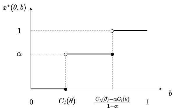
Figure 4: Optimal allocation $x^{*}$ corresponding to the menu described in Theorem 1.

This contract highlights that rationing can emerge in the healthcare market as a consequence of the insurer’s effort to control its price impact. Specifically, after purchasing an insurance contract, an agent with a disease level within $\left(C_{l}(\theta),\frac{C_{h}(\theta)-\alpha C_{l}(\theta)}{1-\alpha}\right]$ would like to access the full unit of hospital services at the given out-of-pocket cost of $C_{l}(\theta)$ but is constrained by the limit of $\alpha$ imposed by the insurer. Moreover, this result may provide an economic rationale for the restrictions in treatment observed in practice in many insurance contracts.

It is important to distinguish this form of rationing from other types of under-insurance, which typically emerge in models with information frictions, such as adverse selection or moral hazard. In those cases, the insurer raises the OPC to limit access to insurance. While this approach is also feasible in our model, the designer instead opts to restrict access to hospital services to reduce insurance coverage. This effect arises solely from the insurer’s attempt to manage its price impact. Notably, in the absence of the equilibrium constraint, the optimal contract for each risk type would always consist of a posted OPC.

Note that although the OPCs offered by an optimal contract may depend on $\theta$, the treatment restriction does not. That is, all contracts that restrict treatment impose the same cap on hospital services—up to $\alpha$ units—regardless of the agent’s risk type.

In Section 3.4, we provide an example with only two risk types that captures the main economic forces leading to Theorem 1, while the complete proof is in Appendix A. To solve the technical challenges that arise in the infinite-dimensional risk-type space, we proceed in two steps. First, we express the insurer’s problem in the quantity space, which is a common technique in mechanism design. However, unlike most problems, we also have a second layer of private information, which is also infinite-dimensional—the agent’s disease level. To address this, we further transform the insurer’s problem into one that closely resembles an optimal transport problem. In this formulation, the insurer matches different risk types with units demanded for hospital services. Then, leveraging known duality results from optimal transport theory, we derive several properties of the solutions to the insurer’s problem, including Theorem 1.

Finally, we must check when the optimal menu is fully implementable. That is, we have to verify when $x^{*}$ satisfies 3.1. In the next section, where we provide an example illustrating the intuition behind Theorem 1, we also establish a sufficient condition on the model primitives that guarantees $x^{*}$ satisfies 3.1.

3.4 Intuition for Theorem 1

In this section, we illustrate the main intuition behind Theorem 1 with an example. Specifically, we consider a setting with only two risk types, $\theta\in\{\theta_{L},\theta_{H}\}$, where $\theta_{H}>\theta_{L}$. This simplified case already reveals the economic forces that drive the insurer to offer contracts with at most two options and explains why one of these options may cap treatment or ration hospital services.

We begin by reformulating the insurer’s problem in the quantity (or quantile) space, a common technique in mechanism design (see, for instance, Dworczak et al., 2021). For this purpose, let $H_{\theta}(\cdot\lvert p):[0,p]\rightarrow[0,1]$ denote the distribution of disease levels for risk type $\theta$, conditional on being strictly greater than $0$ and less than or equal to $p$. Specifically,

$$H_{\theta}(b\mid p)=\frac{H_{\theta}(b)-H_{\theta}(0)}{H_{\theta}(p)-H_{\theta}(0)},$$

By our assumption on $H_{\theta}$, it follows that $H_{\theta}(\cdot\mid p)$ is invertible. Any non-decreasing, left-continuous function $x(\theta,\cdot):[0,p]\rightarrow[0,1]$ can then be represented as:

$$x(\theta,b)=\int_{0}^{1}\mathbf{1}_{[b>b_{\theta}(q)]}\,dG_{\theta}(q),$$

where $b_{\theta}(q)=H_{\theta}^{-1}(1-q\mid p)$ and $G_{\theta}$ is a distribution over $[0,1]$.

Economically, this representation allows us to express a mechanism in the quantity space. In the absence of insurance, only the agents with a disease level exceeding $p$ attend the hospital. As a result, the total demand for hospital services, conditional on risk type $\theta$, is given by $1-H_{\theta}(p)$. To induce additional demand of $[H_{\theta}(p)-H_{\theta}(0)]q$ units, the insurer can offer a simple contract of the form $\{(1,b_{\theta}(q))\}$. Under this contract, in addition to agents with disease levels greater than $p$, those with disease levels in the range $\left(b_{\theta}(q),p\right]$ will also seek hospital services. For risk type $\theta$, the mass of agents within the interval $\left(b_{\theta}(q),p\right]$ corresponds precisely to $[H_{\theta}(p)-H_{\theta}(0)]q$. In other words, the insurer can only influence the demand of agents with disease levels within $(0,p]$. Among these agents, the insurer selects a fraction $q$ who will attend the hospital. Moreover, by appropriately randomizing over $q$ (or equivalently, over simple contracts), the insurer can replicate any feasible demand schedule $x(\theta,\cdot)$. Thus, without loss of generality, the optimization can be performed over $G_{\theta}$ instead of directly over $x(\theta,\cdot)$.

The insurer’s problem in the quantity space is given by:

$$\max_{G}\quad\int_{0}^{1}\Phi(\theta_{L},q)\,dG_{\theta_{L}}(q)\hat{f}(\theta_{L})+\int_{0}^{1}\Phi(\theta_{H},q)\,dG_{\theta_{H}}(q)\hat{f}(\theta_{H})$$

$$\text{s.t.}\quad\int_{0}^{1}q\,dG_{\theta_{L}}(q)\hat{f}(\theta_{L})+\int_{0}^{1}q\,dG_{\theta_{H}}(q)\hat{f}(\theta_{H})=RS(p),$$

where

$$\Phi(\theta,q)=\int_{0}^{q}\phi(\theta,s)ds,$$

$$\phi(\theta_{L},q)=b_{\theta_{L}}(q)-p+\frac{H_{\theta_{L}}(b_{\theta_{L}}(q))-g(H_{\theta_{L}}(b_{\theta_{L}}(q)))}{h_{\theta_{L}}(b_{\theta_{L}}(q))}+\frac{1-f(\theta_{L})}{f(\theta_{L})h_{\theta_{L}}(b_{\theta_{L}}(q))}g(H_{\theta_{H}}(b_{\theta_{H}}(q)))-g(H_{\theta_{L}}(b_{\theta_{L}}(q))),$$

$$\phi(\theta_{H},q)=b_{\theta_{H}}(q)-p+\frac{H_{\theta_{H}}(b_{\theta_{H}}(q))-g(H_{\theta_{H}}(b_{\theta_{H}}(q)))}{h_{\theta_{H}}(b_{\theta_{H}}(q))},$$

$$RS(p)=S(p)-f(\theta_{L})(1-H_{\theta_{L}}(p))-f(\theta_{H})(1-H_{\theta_{H}}(p)),$$

and

$$\hat{f}(\theta)=\left[H_{\theta}(p)-H_{\theta}(0)\right]f(\theta).$$

Observe that $\phi(\theta,q)$ accounts for the period 1 and period 2 virtual values expressed in the quantity space, with the key difference that, since we now consider a discrete risk type space, the period 1 virtual value must be adjusted. Specifically, we account for the discrete version of information rents. These rents no longer arise from the envelope formula but instead follow from the standard result that, with two types, the 3.1 constraint for the high type and the 3.1 constraint for the low type always bind.

We now analyze the insurer’s problem. For any distribution $G_{\theta}$ that results in an average $q$ given by $q_{\theta}$, there exists a distribution $G^{\prime}_{\theta}$ that preserves the same average $q$ while attaining the concave envelope of $\Phi(\theta,\cdot)$ evaluated at $q_{\theta}$. In other words, let $\overline{\Phi}(\theta,\cdot)$ denote the concave envelope of $\Phi(\theta,\cdot)$. Then, we have:

$$\int_{0}^{1}q\,dG^{\prime}_{\theta}(q)=q_{\theta}=\int_{0}^{1}q\,dG_{\theta}(q),$$

and

$$\int_{0}^{1}\Phi(\theta,q)\,dG^{\prime}_{\theta}(q)=\overline{\Phi}(\theta,q_{\theta})\geq\int_{0}^{1}\Phi(\theta,q)\,dG_{\theta}(q).$$

$G^{\prime}$ weakly increases the insurer’s payoff while still satisfying the 3.1 condition. Thus, we can also express the insurer’s problem as:

$$\max_{q}\quad\overline{\Phi}(\theta_{L},q_{\theta_{L}})\hat{f}(\theta_{L})+\overline{\Phi}(\theta_{H},q_{\theta_{H}})\hat{f}(\theta_{H})$$

$$\text{s.t.}\quad q_{\theta_{L}}\hat{f}(\theta_{L})+q_{\theta_{H}}\hat{f}(\theta_{H})=RS(p),$$

In the above formulation, for each risk type, the insurer selects the fraction of agents with a disease level in $(0,p]$ who go to the hospital, denoted by $q_{\theta}$. This formulation already demonstrates why a solution exists in which the contract offered to each risk type includes at most two options. Indeed, any point in $\overline{\Phi}(\theta,\cdot)$ can be attained by a distribution $G_{\theta}$ with at most two elements in its support. This, in turn, results in an allocation function $x(\theta,\cdot)$ with at most two jumps, as illustrated in Figure 4.

Moreover, if $\Phi(\theta,\cdot)$ is concave, or equivalently, $\frac{\partial\phi(\theta,q)}{\partial q}\leq 0$ for all $q$, then the insurer can always achieve $\overline{\Phi}(\theta,q_{\theta})$ with a distribution that puts probability one on $q_{\theta}$. That is, the insurer can always offer risk type $\theta$ the simple contract $\{(1,b_{\theta}(q_{\theta}))\}$. This observation allows us to find sufficient conditions on the model primitives for a risk type to get a simple contract:

Corollary 1 (Simple Contracts)

Fix any risk type $\theta$ and suppose that $\frac{\partial\phi(\theta,q)}{\partial q}\leq 0$ for all $q$. Then, risk type $\theta$ gets a simple contract of the form $\{(1,C(\theta))\}$, where $C(\theta)\in[0,p]$.

In Appendix A, we provide a formal proof of Corollary 1 for the case where the risk-type space is infinite-dimensional.

Nonetheless, a question remains: When does the insurer include a second option that rations hospital services or places a cap on treatment? To illustrate the economic forces that lead the insurer to include this option, we assume $\theta_{L}=0.25$, $\theta_{H}=0.35$, $f(\theta_{H})=\frac{1}{5}$, and $H_{\theta}(b)=1-\theta+\theta Q(b)$, where $Q(b)=b^{2}\cdot\mathbf{1}_{\left[0\leq b\leq 1\right]}$. In this case, we have $q\Phi(\theta,1)>\Phi(\theta,q)$ for all $q\in(0,1)$. This implies that the concave envelope of $\Phi(\theta,\cdot)$ is the line segment connecting $\Phi(\theta,0)$ and $\Phi(\theta,1)$, i.e., $\overline{\Phi}(\theta,q)=q\Phi(\theta,1)$, as shown in Figure 5.

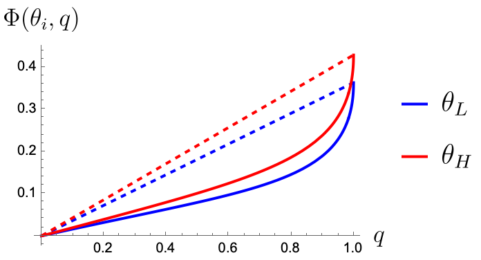
Figure 5: The continuous lines illustrate $\Phi(\theta_{L},q)$ (in blue) and $\Phi(\theta_{H},q)$ (in red). The dashed lines are the respective concave envelopes. The figure is drawn assuming that $p=0.8$.

Under these parametric assumptions, the insurer solves:

$$\max_{q}\quad q_{\theta_{L}}\Phi(\theta_{L},1)\hat{f}(\theta_{L})+q_{\theta_{H}}\Phi(\theta_{H},1)\hat{f}(\theta_{H})$$

$$\text{s.t.}\quad q_{\theta_{L}}\hat{f}(\theta_{L})+q_{\theta_{H}}\hat{f}(\theta_{H})=RS(p).$$

The solution thus depends solely on the relationship between $\Phi(\theta_{L},1)$ and $\Phi(\theta_{H},1)$. In particular, we can verify that $\Phi(\theta_{H},1)>\Phi(\theta_{L},1)$. Therefore, the optimal allocation is:

$$q^{*}_{\theta_{H}}=\min\left\{1,\frac{RS(p)}{\hat{f}(\theta_{H})}\right\},\quad q^{*}_{\theta_{L}}=\frac{RS(p)}{\hat{f}(\theta_{L})}-\min\left\{1,\frac{RS(p)}{\hat{f}(\theta_{H})}\right\}\cdot\frac{\hat{f}(\theta_{H})}{\hat{f}(\theta_{L})}.$$

In other words, the insurer favors the riskier type, allocating as many hospital service units as possible to $\theta_{H}$ first. If the maximum insurance-driven demand, $\hat{f}(\theta_{H})$, is sufficient to meet the residual supply, then $q^{*}_{\theta_{H}}=RS(p)/\hat{f}(\theta_{H})$ and $q^{*}_{\theta_{L}}=0$. Otherwise, we set $q^{*}_{\theta_{H}}=1$ and further increase demand by including some low-risk types until the market clears.

Furthermore, if $q^{*}_{\theta}\in(0,1)$, rationing emerges in the healthcare market. To achieve such $q^{*}_{\theta}$, the insurer mixes between the two extremes of $q=0$ and $q=1$, corresponding to out-of-pocket costs of $p$ and $0$, respectively. For instance, if $p=0.8$, we obtain $q^{*}_{\theta_{L}}=0.67$ and $q^{*}_{\theta_{H}}=1$. In this case, the high-risk type receives full treatment at zero cost, while the low-risk type faces two options: she can access up to 67% of hospital services for free or receive full treatment for an OPC equal to 0.26. Note that individuals choosing the former option are subject to rationing—although they would prefer to access the full unit of hospital services for free, they are constrained by the cap on treatment.

This example also illustrates that rationing in this model arises solely from the insurer’s effort to manage its price impact. If we ignored the equilibrium constraint, the optimal choice under these assumptions would simply be $q_{\theta}=1$ for all $\theta$. In other words, without the equilibrium constraint, full insurance coverage would be provided to both types.

Additionally, since the insurer always favors the riskier type, the optimal menu satisfies 3.1. Indeed, in this case, it is easy to verify that whenever the high-risk type receives a contract that includes an option that places a cap on treatment, the low-risk type receives no insurance. Moreover, whenever the low-risk type receives some form of insurance, the high-risk type gets full insurance—access to the full unit of hospital services at zero cost. Thus, the optimal allocation of hospital services is increasing in the risk type. That is, $x^{*}(\theta_{H},b)\geq x^{*}(\theta_{L},b)$ for all $b$. Therefore, by Lemma 4, Condition (2), we conclude that $x^{*}$ satisfies 3.1.

The economic forces that lead the insurer to favor the riskier type follow from the fact that the profits of providing any units of hospital services are higher for the high-risk type than for the low-risk type, as illustrated in Figure 5. The latter occurs because $\phi(\theta_{H},q)>\phi(\theta_{L},q)$, i.e., the sum of the period 1 and period 2 virtual values is higher for the high-risk type than for the low-risk type for any $q$. We can extend this intuition to the infinite-dimensional risk-type space case:

Corollary 2

Suppose that $\frac{\partial\phi(\theta,q)}{\partial\theta}>0$ for all $\theta$ and $q$. Then, any $x^{*}$ that solves $P$ satisfies 3.1.

The proof of Corollary 2 is in Appendix A.

4 Second Stage: Price of Hospital Services

In the previous section, we took the price of hospital services, $p$, as given and characterized the shape of the optimal menu that sustains $p$ in equilibrium. This allowed us to associate each achievable $p$ with the corresponding profits obtained by the insurer, denoted by $\Pi(p)$.

Now, we proceed to the second-stage analysis, which consists of solving for the price that maximizes these profits. To facilitate the analysis, we assume that the condition imposed by Corollary 1 holds for all $\theta$. That is:

$$\frac{\partial\phi(\theta,q)}{\partial q}\leq 0\quad\text{for all $\theta$ and $q$}.$$

Recall that this condition implies that each risk type $\theta$ receives a simple contract of the form $\{(1,C_{p}(\theta))\}$, where, with a slight abuse of notation, we now explicitly indicate the dependence of the single OPC on the hospital price $p$.

A standard envelope argument (see Milgrom and Segal, 2002) yields the following result:

Theorem 2

Suppose that $\frac{\partial\phi(\theta,q)}{\partial q}\leq 0$ for all $\theta$ and $q$. Then, $\Pi:\left[p^{N},p^{F}\right]\rightarrow\mathbb{R}_{+}$ is differentiable in $p$ and its derivative is given by:

$$\Pi^{\prime}(p)= \int_{\underline{\theta}}^{\overline{\theta}}\mathbf{1}_{\left[C_{p}(\theta)<p\right]}\left[\underbrace{1-g(H_{\theta}(p))+\frac{1-F(\theta)}{f(\theta)}g^{\prime}(H_{\theta}(p))\frac{\partial H_{\theta}(p)}{\partial\theta}}_{\text{Surplus extracted from agents}}-\underbrace{\left(1-H_{\theta}(C_{p}(\theta))\right)}_{\text{Higher payouts}}\right]f(\theta)d\theta$$

$$-\underbrace{\lambda^{*}(p)\left[S^{\prime}(p)+\int_{\underline{\theta}}^{\overline{\theta}}\mathbf{1}_{\left[C_{p}(\theta)=p\right]}h_{\theta}(p)f(\theta)d\theta\right]}_{\text{Equilibrium effects}},$$

where $C_{p}(\theta)$ is the single OPC in the optimal simple contract offered to risk type $\theta$, and $\lambda^{*}(p)$ is a multiplier that captures the value of relaxing the equilibrium constraint.

For a proof demonstrating the existence of $\lambda^{*}$, see the proof of Theorem 1. There, we derive a dual to the insurer’s problem, for which we prove the existence of a solution and the absence of a duality gap. The solution to this dual problem includes $\lambda^{*}$.

The theorem identifies three forces that determine the value of inducing a marginally higher price in the hospital market. For each $\theta$, the term $1-g(H_{\theta}(p))$ captures the increase in the value of insurance for agents ex ante. They now face a riskier outside option (if they get sick and want to visit a hospital, they have to pay a higher price), which increases their willingness to pay for insurance.

If $\theta$ were common knowledge, the insurer would be able to appropriate the entirety of this surplus by increasing premiums (and hence profits) by the same amount. However, when $\theta$ is private information, the insurer can only appropriate the surplus net of first-period information rents (recall that $\frac{1-F(\theta)}{f(\theta)}g^{\prime}(H_{\theta}(b))\frac{\partial H_{\theta}(b)}{\partial\theta}$ is negative).

The second term, $1-H_{\theta}(C_{p}(\theta))$, captures the cost to the insurer of increasing the price. Indeed, if risk type $\theta$ has the simple contract $\{(1,C_{p}(\theta))\}$, then all agents with a disease level in the range $(C_{p}(\theta),\bar{b}]$ will opt for attending the hospital and paying the OPC $C_{p}(\theta)$. This leads to a total demand equal to $1-H_{\theta}(C_{p}(\theta))$. Therefore, a unit price increase causes an increase in payouts by the same amount.

Both effects in the first bracket are only present if the optimal contract provides insurance to type $\theta$. Since no provision of insurance is represented by a simple contract with an OPC of $C_{p}(\theta)=p$, we capture this using the indicator $\mathbf{1}_{\left[C_{p}(\theta)<p\right]}$.

Finally, we must account for equilibrium effects. The sign of this component is determined by the sign of the multiplier, since the term inside the brackets is always positive and captures the increase in residual supply. Specifically, an increase in prices leads to an increase in the supply of hospital services, captured by $S^{\prime}(p)$. It also causes a reduction in demand among those who do not receive insurance under the optimal contract (i.e., for whom $C_{p}(\theta)=p$).

Next, we introduce the concept of a price-taking benchmark, which is obtained by solving problem $P$ while ignoring the 3.1 constraint. In this case, the optimal contract always takes the form of a simple contract. Moreover, if we maintain the condition imposed in Corollary 1, it follows that the single OPC in a type $\theta$ contract is given $C_{p}(\theta)=J^{-1}_{p}(\theta,0)$ and the corresponding optimal $x$ is given by $x^{U}(\theta,b)=\mathbf{1}_{\left[b>J^{-1}_{p}(\theta,0)\right]}$, where $J^{-1}_{p}(\theta,0)$ represents the inverse of $J$ —the sum of the period 1 and period 2 virtual values— with respect to $b$, evaluated at 0 (the notation now explicitly indicates the dependence of $J$ on $p$). Substituting this $x^{U}$ into the 3.1 constraint allows us to solve for the resulting equilibrium price $p^{U}$. We refer to this as the price-taking benchmark because $p^{U}$ is the market price that would emerge if the insurer took the price as given and did not internalize his impact on the market for hospital services.

Importantly, the value of relaxing the equilibrium constraint at $p^{U}$ is zero, i.e., $\lambda^{*}(p^{U})=0$. This enables us to assess whether there are local incentives to provide more or less insurance relative to the price-taking benchmark. Specifically, by evaluating $\Pi^{\prime}$ at $p^{U}$ we obtain:

$$\int_{\underline{\theta}}^{\overline{\theta}}\mathbf{1}_{\left[J_{p^{U}}^{-1}(\theta,0)<p^{U}\right]}\left[H_{\theta}\left(J_{p^{U}}^{-1}(\theta,0)\right)-g(H_{\theta}(p^{U}))+\frac{1-F(\theta)}{f(\theta)}g^{\prime}(H_{\theta}(p^{U}))\frac{\partial H_{\theta}(p^{U})}{\partial\theta}\right]f(\theta)d\theta.$$

If the above term is positive (negative), there are local incentives to increase (reduce) the price above (below) $p_{U}$ and thus provide more (less) insurance compared to the price-taking benchmark. That is, if the additional surplus that the insurer can extract by making the agents’ outside option worse is higher (lower) than the increase in payouts, then in a small neighborhood around $p^{U}$ the insurer prefers a price $p>(<)p^{U}$.

As we demonstrate with an example, it is possible to compute the multiplier numerically and verify whether the resulting $\Pi^{\prime}$ is decreasing in $p$. When this condition holds, Theorem 2 can be used to determine the optimal price by identifying the $p^{*}$ such that $\Pi^{\prime}(p^{*})=0$. Furthermore, the term that indicates whether the insurer has local incentives to raise or decrease the price relative to the price-taking benchmark now captures these incentives globally.

Let $\theta\sim U[0,1]$, $H_{\theta}(b)=1-\theta+\theta Q(b)$, and $Q(b)=b\cdot\mathbf{1}_{\left[0\leq b\leq 1\right]}$. Furthermore, for simplicity let us assume that the risk type $\theta$ of the agent is common knowledge. Then, $\Pi^{\prime}(p)$ is as shown in Figure 6:

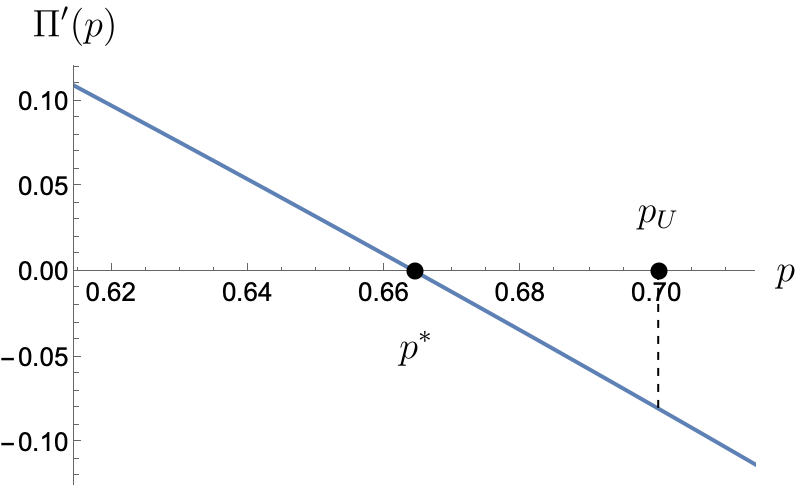
Figure 6: $\Pi^{\prime}(p)$ for $\theta\sim U[0,1]$, $H_{\theta}(b)=1-\theta+\theta Q(b)$, and $Q(b)=b\cdot\mathbf{1}_{\left[0\leq b\leq 1\right]}$. In this case, the optimal price $p^{*}=0.66$ and $p^{U}=0.7$

Note that $\Pi^{\prime}(p)$ is decreasing and $\Pi^{\prime}(p^{U})<0$. Therefore, the optimal price $p^{*}$ is smaller than $p^{U}$ and we have under-insurance compared to the price-taking benchmark.

5 Conclusion

We examined the problem of a monopolistic insurer contracting with a population of agents who are risk-averse in the sense of Yaari (1987) and face the risk of developing an illness, which can be cured by a hospital at the prevailing market price. Departing from standard models of insurance, we explicitly account for the fact that insurance contracts affect agents’ demand for hospital services, which in turn influences the market price. Since the price determines both the cost of providing insurance and the surplus that can be extracted through premiums, large insurers are likely to internalize their price impact when choosing the profit-maximizing contracts, with an effect on both the shape of the contracts offered to agents and on the amount of insurance provided.

We show in Theorem 1, that the optimal contracts contain at most two options: one that provides full hospital coverage at a high out-of-pocket cost, and the other offering restricted coverage at a low out-of-pocket cost. This finding highlights a novel form of under-insurance—the rationing of healthcare services—which arises from the insurer’s attempt to control his price impact.

Our second main result, presented in Theorem 2, highlights the role of healthcare prices in determining the incentives of the insurer to provide coverage. Higher prices increase insurer payouts but also worsen the agents’ outside options, thereby raising their willingness to pay for insurance ex ante. The interplay between these forces ultimately determines whether the equilibrium provision of insurance exceeds or falls short of a price-taking benchmark.

Appendix A Proof of Theorem 1

In this section we provide the main steps and ideas behind the proof of Theorem 1, Corollary 1 and Corollary 2. However, we relegate all technical proofs to Appendix D.

Step 1: Representing Problem $P$ in the Quantity space.

As in the two-type case in Section 3.4, the first step in proving Theorem 1 is to reformulate the insurer’s problem $P$ in the quantity space. To make this reformulation self-contained, we revisit the main steps and introduce the key objects that allow us to represent the problem in this way. Let $H_{\theta}(\cdot\lvert p):[0,p]\rightarrow[0,1]$ denote the distribution of disease levels for risk type $\theta$, conditional on being strictly greater than $0$ and less than or equal to $p$. Specifically,

$$H_{\theta}(b\mid p)=\frac{H_{\theta}(b)-H_{\theta}(0)}{H_{\theta}(p)-H_{\theta}(0)},$$

By our assumption on $H_{\theta}$, it follows that $H_{\theta}(\cdot\mid p)$ is invertible. Any non-decreasing, left-continuous function $x(\theta,\cdot):[0,p]\rightarrow[0,1]$ can then be represented as:

$$x(\theta,b)=\int_{0}^{1}\mathbf{1}_{[b>b_{\theta}(q)]}\,dG_{\theta}(q),$$

where $b_{\theta}(q)=H_{\theta}^{-1}(1-q\mid p)$ and $G_{\theta}$ is a distribution over $[0,1]$.

Thus, without loss of generality, the optimization can be performed over $G_{\theta}$ instead of directly over $x(\theta,\cdot)$. Then, the insurer’s problem becomes:

$$\max_{G}\quad\int_{\underline{\theta}}^{\bar{\theta}}\int_{0}^{1}\Phi(\theta,q)\,dG_{\theta}(q)f(\theta)\,d\theta, P^{\prime}$$ ()

$$\text{s.t.}\quad\int_{\underline{\theta}}^{\bar{\theta}}\int_{0}^{1}[H_{\theta}(p)-H_{\theta}(0)]q\,dG_{\theta}(q)f(\theta)\,d{\theta}=RS(p), EQ$$ ()

where

$$\Phi(\theta,q)=[H_{\theta}(p)-H_{\theta}(0)]\int_{0}^{q}\phi(\theta,s)ds,$$

and

$$\phi(\theta,q)=\left[1-g(H_{\theta}(b_{\theta}(q)))+\frac{1-F(\theta)}{f(\theta)}g^{\prime}(H_{\theta}(b_{\theta}(q)))\frac{\partial H_{\theta}(b_{\theta}(q))}{\partial\theta}\right]\frac{1}{h_{\theta}(b_{\theta}(q))}+b_{\theta}(q)-p-\frac{1-H_{\theta}(b_{\theta}(q))}{h_{\theta}(b_{\theta}(q))}.$$

Step 2: Optimal Transport and Duality.

Consider a collection of distributions over $[0,1]$, denoted by $\{G_{\theta}\}_{\theta\in\Theta}$, which the insurer selects in problem $P^{\prime}$. Additionally, recall that $F$ denotes the prior distribution over risk types. Together, these define a probability measure $\pi$ on $\Theta\times[0,1]$, where the marginal of $\pi$ on $\Theta$ is $F$. We can then reformulate problem $P^{\prime}$ as follows:

$$\max_{\pi}\quad\int_{\underline{\theta}}^{\bar{\theta}}\int_{0}^{1}\Phi(\theta,q)\,d\pi(\theta,q) OT$$ ()

$$\text{s.t.}\quad\int_{0}^{\theta}\int_{0}^{1}\,d\pi(s,q)=F(\theta),\quad\forall\theta\in\Theta, BP$$ ()

$$\;\;\;\;\;\;\;\int_{\underline{\theta}}^{\bar{\theta}}\int_{0}^{1}[H_{\theta}(p)-H_{\theta}(0)]q\,d\pi(\theta,q)=RS(p). EQ$$ ()

In the primal problem $OT$, the insurer selects a joint distribution of risk types and quantities demanded for hospital services. This formulation is particularly useful because it has a strong resemblance to an optimal transport problem.

More precisely, the insurer is effectively matching risk types to hospital service demands. If risk type $\theta$ is matched with $q$, then among the agents that the insurer can influence to attend the hospital—those with a disease level in the range $(0,p]$—a fraction $q$ will seek hospital care. However, this allocation is subject to two constraints. The first constraint, $BP$, ensures that the insurer does not assign more individuals of risk type $\theta$ than the total available, as determined by the prior distribution $F$. In other words, the marginal of $\pi$ on $\Theta$ must coincide with $F$, mirroring a Bayes-plausibility constraint in Bayesian persuasion models. The second constraint, 3.1, is the equilibrium condition described earlier.

The similarity between $OT$ and an optimal transport problem is advantageous because it allows us to leverage known duality results to analyze the insurer’s optimization problem more effectively. To this end, we introduce the corresponding dual problem:

$$\min_{v,\lambda}\quad\int_{\underline{\theta}}^{\bar{\theta}}v(\theta)f(\theta)d\theta D$$ ()

$$\text{s.t.}\quad v(\theta)\geq\max_{q\in[0,1]}\;\Phi(\theta,q)+\lambda\left([H_{\theta}(p)-H_{\theta}(0)]q-RS(p)\right),\quad\text{for $f$-almost all $\theta$}. SP$$ ()

In this dual formulation, $v(\theta)$ represents the shadow price of matching risk type $\theta$ with $q$. The multiplier $\lambda$ corresponds to the marginal value of relaxing the equilibrium constraint 3.1. Furthermore, constraint $SP$ ensures that $v(\theta)$ is at least as large as the insurer’s valuation of matching risk type $\theta$ to $q$, where this valuation consists of the insurer’s profit, $\Phi(\theta,q)$, plus the term multiplied by $\lambda$, which captures the excess demand or supply generated by risk type $\theta$ when assigned to $q$.

Then, we have the following duality result:

Theorem 3 (Monge-Kantorovich Duality)

A solution tho both the primal problem $OT$ and the dual problem $D$ exists. Furthermore, there is no duality gap: the optimal value of the primal problem $OT$ equals the optimal value of the dual problem $D$.

The formal proof of Theorem 3 can be found in Appendix D.

The absence of a duality gap is a direct consequence of the Monge-Kantorovich duality in optimal transport problems (see, for example, Villani et al., 2009). The existence of a solution to the primal problem $OT$ follows from our technical assumptions on $H_{\theta}$ that guarantee the continuity of the function $\Phi$ and the fact that the maximization is performed over a compact space. Finally, leveraging the absence of a duality gap and the existence of a solution to the primal problem, we explicitly construct a solution to the dual problem $D$.

Step 3: Implications of Zero Duality Gap.

An immediate consequence of the absence of a duality gap is that, given a solution to the dual problem $D$, we obtain necessary and sufficient conditions that any joint distribution $\pi$ must satisfy to be a solution of the primal problem $OT$. To establish these conditions, consider any $\pi$ that satisfies $BP$. Let $\pi(\cdot\mid\theta)$ denote the distribution over $[0,1]$ conditional on risk type $\theta$, defined as:

$$\pi(q\mid\theta)=\frac{\pi(q,\theta)}{f(\theta)}.$$

With this, we obtain the following complementary slackness result:

Corollary 3 (Complementary Slackness)

Suppose that $(v^{*},\lambda^{*})$ is a solution to the dual problem $D$. Then, any $\pi$ that satisfies conditions $BP$ and 3.1 is a solution to the primal problem $OT$ if and only if $f$-almost every $\theta$ has $\pi(\cdot\mid\theta)$ supported on

$$\arg\max_{q\in[0,1]}\quad\Phi(\theta,q)+\lambda^{*}\left([H_{\theta}(p)-H_{\theta}(0)]q-RS(p)\right).$$

The formal proof of Corollary 3 is in Appendix D.

The proof of Corollary 3 follows directly from the absence of a duality gap and the fact that if $(v^{*},\lambda^{*})$ is a solution to $D$, then we have

$$v^{*}(\theta)=\max_{q\in[0,1]}\quad\Phi(\theta,q)+\lambda^{*}\left([H_{\theta}(p)-H_{\theta}(0)]q-RS(p)\right),$$

where the maximum is well-defined due to the continuity of $\Phi(\theta,\cdot)$ and the compactness of the set $[0,1]$.

Corollary 3 is particularly useful for proving Theorem 1, Corollary 1, and Corollary 2. We begin by examining its implications for Theorem 1. To this end, we introduce the following lemma, from which Theorem 1 follows immediately:

Lemma 8 (Solution to $OT$)

There exists a $\pi^{*}$ that is a solution to the primal problem $OT$ and, for all $\theta$ and $q$, $\pi^{*}(q\mid\theta)\in\{0,\alpha,1\}$ for some $\alpha\in(0,1)$.

The proof of Lemma 8 in Appendix D.

Theorem 1 follows directly from Lemma 8. Once we know that $\pi^{*}$ is a solution to the primal problem $OT$, it immediately implies that the following function $x^{*}$ solves the insurer’s problem $P$:

$$x^{*}(\theta,b)=\int_{0}^{1}\mathbf{1}_{\left[b>b_{\theta}(q)\right]}\,d\pi^{*}(q\mid\theta).$$

Since $\pi^{*}(\cdot\mid\theta)$ consists of at most two jumps, and the size of these jumps is independent of the risk type, $x^{*}$ has the form shown in Figure 4.

The intuition behind the proof of Lemma 8 is as follows: By Theorem 3 and Corollary 3, we know that there exists a $\pi^{\prime}$ that solves $OT$, a $(v^{*},\lambda^{*})$ that solves $D$, and that $\pi^{\prime}(\cdot\mid\theta)$ is supported on 3.

By Carathéodory’s theorem, we can construct a new distribution $\pi^{\prime\prime}$ such that $\operatorname{supp}\pi^{\prime\prime}(\cdot\mid\theta)$ contains at most two elements, is a subset of $\operatorname{supp}\pi^{\prime}(\cdot\mid\theta)$, and results in the same average quantity of hospital services for type $\theta$. This implies that $\pi^{\prime\prime}$ still satisfies the 3.1 constraint. Furthermore, since $\operatorname{supp}\pi^{\prime\prime}(\cdot\mid\theta)\subset\operatorname{supp}\pi^{\prime}(\cdot\mid\theta)$, we can again apply Corollary 3 to conclude that $\pi^{\prime}$ is optimal.

However, we can extend this further. Since the 3.1 constraint is satisfied by ensuring the sum of the average quantities across risk types equals the residual supply, we can construct another distribution, $\pi^{*}$, that preserves the same support as $\pi^{\prime\prime}$, makes the size of the jumps independent of the risk type, and ensures the sum of the average quantities across risk types (though not necessarily the average quantities themselves) is preserved. This $\pi^{*}$ still satisfies 3.1, and because the supports are identical, we can apply Corollary 3 again to conclude that $\pi^{*}$ is also optimal.

Next, we examine the implications of our complementary slackness result for Corollary 1:

Lemma 9 (Simple Contracts)

Fix any risk type $\theta$ and suppose that $\frac{\partial\phi(\theta,q)}{\partial q}\leq 0$ for all $q$. Furthermore, let $\pi^{*}$ be the solution to the primal problem $OT$ described in Lemma 8. Then, $\pi^{*}(q\mid\theta)\in\{0,1\}$ for all $q$.

The proof of Lemma 9 is provided in Appendix D.

Corollary 1 follows immediately from Lemma 9. Since $\pi^{*}(\cdot\mid\theta)$ places probability 1 on a single $q$, the contract for risk type $\theta$ is a simple contract.

Lemma 9 once again relies on our complementary slackness result. To illustrate, suppose that $\frac{\partial\phi(\theta,q)}{\partial q}>0$ holds with strict inequality. Then, the objective in 3 is strictly concave in $q$, implying that the set 3 contains only one element. Moreover, by our complementary slackness result, we know that $\pi^{*}(\cdot\mid\theta)$ is supported on 3, leading to the desired conclusion.

Finally, we turn to the implications of our complementary slackness result for Corollary 2:

Lemma 10

Suppose that $\frac{\partial\phi(\theta,q)}{\partial\theta}>0$ for all $q$ and let $\pi^{*}$ be a solution to the primal problem. Then, for any $\theta>\theta^{\prime}$, we have

$$\min\operatorname{supp}\pi^{*}(\cdot\mid\theta)\geq\max\operatorname{supp}\pi^{*}(\cdot\mid\theta^{\prime}).$$

The proof of Lemma 10 is provided in Appendix D.

Lemma 10 implies that the allocation $x^{*}$ obtained through $\pi^{*}$, which solves the insurer’s problem $P$, satisfies the monotonicity condition: $x^{*}(\cdot,b)$ is non-decreasing for all $b$. Therefore, by Lemma 4 and Condition (2), $x^{*}$ satisfies 3.1.

The intuition behind Lemma 10 is straightforward. By Corollary 3, we know that $\pi^{*}(\cdot\mid\theta)$ is supported on 3. Then, applying Topkis’s monotonicity theorem, we conclude that the objective in 3 strictly increases in $\theta$ in the strong set order, yielding the desired result.

Appendix B Proofs of results in Section 3.1

Proof of Lemma 1. Suppose that a contract satisfies $IC_{2}$ and that $C(\theta,b)>b_{p}$ for some $b$. In this case, the agent will not use her insurance and her loss is given by $L(b;\theta)=b_{p}$.

Now, suppose the insurer modifies the contract by setting $C^{\prime}(\theta,b)=b_{p}$ and $x^{\prime}(\theta,b)=0$. Under this modified contract, the loss remains unchanged at $L^{\prime}(b;\theta)=b_{p}$. The treatment cost for the insurer remains equal to 0, the demand for hospital services remains 1 if $b>p$ and 0 otherwise. Finally, for every $b^{\prime}\neq b$, $L^{\prime}(b^{\prime},b;\theta)=b_{p}\geq L(b^{\prime};\theta)$. Therefore, $IC_{2}$ is still satisfied.   

Proof of Lemma 2. Suppose that a contract satisfies $IC_{2}$. Towards a contradiction, assume that $L(b;\theta)>L(p;\theta)$ for some $b>p$. Then:

$$L(b,p;\theta)=x(\theta,p)\min\{C(\theta,p),p\}+(1-x(\theta,p))p=L(p;\theta)<L(b;\theta),$$

which contradicts the assumption that $IC_{2}$ is satisfied. Therefore, we must have $L(b;\theta)\leq L(p;\theta)$. A similar argument shows that $L(b;\theta)\geq L(p;\theta)$, hence $L(p;\theta)=L(b;\theta)$ for all $b>p$.

To see why we can, with out loss of generality, set $x(\theta,b)=1$ for all $b>p$, suppose instead that $x(\theta,b)<1$ for some $b>p$. Consider a modified contract where $x^{\prime}(\theta,b)=1$ and $C^{\prime}(\theta,b)=L(p;\theta)$ for all $b>p$. Then, $L^{\prime}(b;\theta)=\min\{L(p;\theta),p\}=L(p;\theta)=L(b;\theta)$. Thus, the loss remains unchanged. Moreover, $p-C^{\prime}(\theta,b)=p-L(p;\theta)=p-L(b;\theta)=x(\theta,b)(p-C(\theta,b))$, meaning the treatment cost to the insurer also remains the same. The demand for hospital services is still 1. Finally, for any $b\leq p$, we have:

$$L(b;\theta) \leq L(b,p;\theta)\leq x(\theta,p)\min\{C(\theta,p),p\}+(1-x(\theta,p))p=L(p;\theta).$$

Additionally, we know that $L(b;\theta)\leq b$. Hence, $L(b;\theta)\leq\min\{L(p;\theta),b\}$. Since $L^{\prime}(b,p;\theta)=\min\{L(p;\theta),b\}$, $IC_{2}$ is still satisfied.   

Proof of the Necessity part of Lemma 3. Suppose that a contract satisfies $IC_{2}$. Then, for any $b,b^{\prime}\in[0,p]$, we have:

$$L(b;\theta)\leq L(b,b^{\prime};\theta)=(1-x(\theta,b^{\prime}))b+x(\theta,b^{\prime})\min\{C(\theta,b^{\prime}),b\}\leq(1-x(\theta,b^{\prime}))b+x(\theta,b^{\prime})C(\theta,b^{\prime}).$$

Thus:

$$L(b;\theta)=\min_{b^{\prime}\in[0,p]}\;\;x(\theta,b^{\prime})C(\theta,b^{\prime})+(1-x(\theta,b^{\prime}))b.$$

Using the envelope theorem (see Milgrom and Segal, 2002), it follows that:

$$L(b;\theta)=L(0;\theta)+\int_{0}^{b}(1-x(\theta,l))\,dl.$$

Furthermore, since $0\leq L(b;\theta)\leq b$, we have $L(0;\theta)=0$. Thus:

$$L(b;\theta)=\int_{0}^{b}(1-x(\theta,l))dl.$$

We now show Condition (2) of Lemma 3. From $IC_{2}$, for $p\geq b>b^{\prime}$, we have:

$$(1-x(\theta,b))b+x(\theta,b)C(\theta,b) \leq(1-x(\theta,b^{\prime}))b+x(\theta,b^{\prime})\min\{C(\theta,b^{\prime}),b\}$$

$$=(1-x(\theta,b^{\prime}))b+x(\theta,b^{\prime})C(b^{\prime},\theta),$$

$$(1-x(\theta,b^{\prime}))b^{\prime}+x(\theta,b^{\prime})C(\theta,b^{\prime}) \leq(1-x(\theta,b))b^{\prime}+x(\theta,b)\min\{C(\theta,b),b^{\prime}\}$$

$$\leq(1-x(\theta,b))b^{\prime}+x(\theta,b)C(b,\theta).$$

If we combine both inequalities we get:

$$(1-x(\theta,b))(b-b^{\prime}) \leq(1-x(\theta,b^{\prime}))(b-b^{\prime})$$

$$x(\theta,b^{\prime}) \leq x(\theta,b).$$

 

Proof of the Sufficiency part of Lemma 3. Suppose a contract satisfies Conditions (1) and (2) of Lemma 3. For $b,b^{\prime}\in[0,p]$ with $b^{\prime}\leq b$, we have:

$$L(b,b^{\prime};\theta) =x(b^{\prime},\theta)C(b^{\prime},\theta)+(1-x(b^{\prime},\theta))b$$

$$=L(b^{\prime};\theta)+(b-b^{\prime})(1-x(\theta,b^{\prime}))$$

$$=\int_{0}^{b^{\prime}}(1-x(\theta,l))\,dl+\int_{b^{\prime}}^{b}(1-x(\theta,b^{\prime}))\,dl$$

$$\geq\int_{0}^{b^{\prime}}(1-x(\theta,l))\,dl+\int_{b^{\prime}}^{b}(1-x(\theta,l))\,dl$$

$$=L(b;\theta),$$

where the inequality follows from Condition (2), and the last equality from Condition (1). This shows $IC_{2}$ is satisfied for $b,b^{\prime}\in[0,p]$ with $b^{\prime}\leq b$.

Similarly, for $b,b^{\prime}\in[0,p]$ with $b\leq b^{\prime}$, $L(b,b^{\prime};\theta)$ can take two possible values. If $C(\theta,b^{\prime})>b$, $L(b,b^{\prime};\theta)=b\geq L(b;\theta)$ and $IC_{2}$ is trivially satisfied. If $C(\theta,b^{\prime})\leq b$, we have:

$$L(b,b^{\prime};\theta) =L(b^{\prime};\theta)-(b^{\prime}-b)(1-x(\theta,b^{\prime}))$$

$$=\int_{0}^{b^{\prime}}(1-x(\theta,l))\,dl-\int_{b}^{b^{\prime}}(1-x(\theta,b^{\prime}))\,dl$$

$$\geq\int_{0}^{b^{\prime}}(1-x(\theta,l))\,dl-\int_{b}^{b^{\prime}}(1-x(\theta,l))\,dl$$

$$=L(b;\theta),$$

This shows $IC_{2}$ is satisfied for $b,b^{\prime}\in[0,p]$ with $b\leq b^{\prime}$.

Next, for $b>p$ and $b^{\prime}\in[0,p]$, we have that $L(b,b^{\prime};\theta)=L(p,b^{\prime};\theta)$ and $L(p;\theta)=L(b;\theta)$. From earlier arguments we know that $L(p;\theta)\leq L(p,b^{\prime};\theta)$. Then, $L(b;\theta)\leq L(b,b^{\prime};\theta)$ and $IC_{2}$ is satisfied for $b>p$ and $b^{\prime}\in[0,p]$.

Finally, for $b\in[0,p]$ and $b^{\prime}>p$, we have that $x(\theta,b^{\prime})=1$ and $L(b^{\prime};\theta)=L(p,\theta)$. Thus, $L(b,b^{\prime};\theta)=\min\{L(p;\theta),b\}$. Furthermore, we know that $L(b;\theta)\leq b$ and that:

$$L(p;\theta) =x(\theta,p)C(\theta,p)+(1-x(\theta,p))p$$

$$\geq x(\theta,p)C(\theta,p)+(1-x(\theta,p))b$$

$$=L(b,p;\theta)$$

$$\geq L(b,\theta),$$

where the last inequality follows from earlier arguments. Therefore, $L(b,;\theta)\leq\min\{L(p;\theta),b\}=L(b,b^{\prime};\theta)$ and $IC_{2}$ is satisfied for $b\in[0,p]$ and $b^{\prime}>p$.   

Proof of Condition (1) of Lemma 4. Suppose that a menu satisfies 3.1. Using the envelope theorem (see Milgrom and Segal (2002)), the agent’s certainty equivalent is given by:

$$U(\theta)=U(\underline{\theta})+\int_{\underline{\theta}}^{\theta}\int_{0}^{p}(1-x(s,b))g^{\prime}(H_{s}(b))\frac{\partial H_{s}(b)}{\partial s}\,db\,ds.$$

 

Proof of Condition (2) of Lemma 4. Suppose that a menu satisfies Condition (1) of Lemma 4 and $x(\cdot,b):B\rightarrow[0,1]$ is a non-decreasing function for every $\theta$. Then, for any $\theta>\theta^{\prime}$, we have that:

$$U(\theta,\theta^{\prime}) =-t(\theta^{\prime})-\int_{0}^{p}(1-x(\theta^{\prime},b))[1-g(H_{\theta}(b))]\,db$$

$$=U(\theta^{\prime})+\int_{0}^{p}(1-x(\theta^{\prime},b))[1-g(H_{\theta^{\prime}}(b))]\,db-\int_{0}^{\bar{b}}(1-x(\theta^{\prime},b))[1-g(H_{\theta}(b))]\,db$$

$$=U(\theta^{\prime})+\int_{\theta^{\prime}}^{\theta}\int_{0}^{p}(1-x(\theta^{\prime},b))g^{\prime}(H_{s}(b))\frac{\partial H_{s}(b)}{\partial s}\,db\,ds$$

$$=U(\theta)+\int_{\theta^{\prime}}^{\theta}\int_{0}^{p}[x(s,b)-x(\theta^{\prime},b)]g^{\prime}(H_{s}(b))\frac{\partial H_{s}(b)}{\partial s}\,db\,ds$$

$$\leq U(\theta),$$

where the second equality follows from the definition of $U(\theta^{\prime})$, while the fourth equality is a consequence of Condition (1). The inequality stems from the assumptions that $x(\cdot,b)$ is a non-decreasing function, $g$ is increasing, and $\frac{\partial H_{\theta}(b)}{\partial\theta}\leq 0$ for all $b$. This last fact arises because $H_{\theta}$ increases in the sense of first-order stochastic dominance. An equivalent argument shows that same inequality holds when $\theta<\theta^{\prime}$.   

Proof of Lemma 1. The necessity part follows trivially. In order to show the sufficiency part, suppose that a menu satisfies 3.1 and that 3.1 holds for type $\underline{\theta}$. The certainty equivalent that type $\theta$ gets from not participating is

$$U_{NP}(\theta) =-\int_{0}^{p}[1-g(H_{\theta}(b))]\,db$$

$$=U_{NP}(\underline{\theta})+\int_{\underline{\theta}}^{\theta}\int_{0}^{p}g^{\prime}(H_{s}(b))\frac{\partial H_{s}(b)}{\partial s}\,db\,ds.$$

Then, by Lemma 4 Condition (1) we get that:

$$U(\theta)-U_{NP}(\theta)=U(\underline{\theta})-U_{NP}(\underline{\theta})-\int_{\underline{\theta}}^{\theta}\int_{0}^{p}x(s,b)g^{\prime}(H_{s}(b))\frac{\partial H_{s}(b)}{\partial s}\,db\,ds.$$

By assumption $U(\underline{\theta})-U_{NP}(\underline{\theta})\geq 0$. Furthermore, $x(\theta,b)\geq 0$, $g$ is increasing and $\frac{\partial H_{\theta}(b)}{\partial\theta}\leq 0$. Hence:

$$\int_{\underline{\theta}}^{\bar{\theta}}\int_{0}^{p}x(s,b)g^{\prime}(H_{s}(b))\frac{\partial H_{s}(b)}{\partial s}\,db\,ds\leq 0.$$

Therefore, $U(\theta)-U_{NP}(\theta)\geq 0$.   

Proof of the Necessity part of Lemma 6. Suppose that for some $x$ satisfying Lemma 3, Condition (2), and some $p\in\mathbb{R}_{+}$, we have $D(p;x)=S(p)$.

Since $D(p;x)\leq 1$, $S\left(p^{F}\right)=1$, and $S(p)$ is strictly increasing, it immediately follows that $p\leq p^{F}$.

Recall that $D(p;x)=S(p)$ can also be expressed as

$$\int_{\underline{\theta}}^{\bar{\theta}}\int_{0}^{p}x(\theta,b)h_{\theta}(b)\,db\,f(\theta)\,d\theta=RS(p).$$

The smallest achievable value on the left-hand side of the equation is zero. For the right-hand side, we know that $R\left(p^{N}\right)=0$, and our technical assumptions imply that $RS(p)$ is strictly increasing. Therefore, the equality cannot hold for any $p<p^{N}$. Thus, $p\geq p^{N}$.   

Proof of the Sufficiency part of Lemma 6. Suppose that $p\in\left(p^{N},p^{F}\right)$, and for any $\alpha\in[0,1]$, define the following function:

$$ED(\alpha;p)=\int_{\underline{\theta}}^{\bar{\theta}}\int_{0}^{p}\alpha h_{\theta}(b)\,db\,f(\theta)\,d\theta-RS(p).$$

Note that $ED(\alpha;p)$ is continuous in $\alpha$ and satisfies $ED(0;p)<0$ and $ED(1;p)>0$. By the intermediate value theorem, there exists an $\alpha^{*}\in(0,1)$ such that $ED(\alpha^{*};p)=0$.

Next, define $x(\theta,b)=\alpha^{*}$ for all $b\in[0,p]$. It follows that $x$ satisfies $IC_{2}$, Condition (2), and 3.1.   

Appendix C Proofs of results in Section 3.2

Proof of Lemma 7. If an agent has risk type $\theta$ and disease level $b$, the insurance provider pays $x(\theta,b)(p-C(\theta,b))$ to the hospital. Furthermore, we know that

$$x(\theta,b)C(\theta,b)=L(b;\theta)-(1-x(\theta,b))b,$$

and by Lemma 3, we have:

$$L(b;\theta)=\int_{0}^{b}(1-x(\theta,l))\,dl\;\text{for all }b\in[0,p],\;L(p;\theta)=L(b;\theta)\text{ for all }b>p,\;\text{and }x(\theta,b)=1\text{ for all }b>p.$$

Thus, the insurer’s cost of providing the contract for risk type $\theta$ simplifies as follows:

$$\int_{0}^{\bar{b}}x(\theta,b)[C(\theta,b)-p]h_{\theta}(b)\,db= \int_{0}^{\bar{b}}x(\theta,b)(b-p)h_{\theta}(b)\,db+\int_{0}^{\bar{b}}(L(b;\theta)-b)h_{\theta}(b)\,db$$

$$= \int_{0}^{p}x(\theta,b)(b-p)h_{\theta}(b)\,db+\int_{p}^{\bar{b}}(b-p)h_{\theta}(b)\,db$$

$$-\int_{0}^{p}\left[\int_{0}^{b}x(\theta,l)\,dl\right]h_{\theta}(b)\,db+\int_{p}^{\bar{b}}(L(p;\theta)-b)h_{\theta}(b)\,db$$

$$= \int_{0}^{p}x(\theta,b)(b-p)h_{\theta}(b)\,db-p(1-H_{\theta}(p))$$

$$-\int_{0}^{p}x(\theta,b)\,dbH_{\theta}(p)+\int_{0}^{p}x(\theta,b)H_{\theta}(b)\,db+\int_{p}^{\bar{b}}L(p;\theta)h_{\theta}(b)\,db$$

$$= \int_{0}^{p}x(\theta,b)(b-p)h_{\theta}(b)\,db-p(1-H_{\theta}(p))$$

$$+(L(p;\theta)-p)H_{\theta}(p)+\int_{0}^{p}x(\theta,b)H_{\theta}(b)\,db+L(p;\theta)(1-H_{\theta}(p))$$

$$= \int_{0}^{p}x(\theta,b)(b-p)h_{\theta}(b)\,db+\int_{0}^{p}x(\theta,b)H_{\theta}(b)\,db+L(p;\theta)-p$$

$$= \int_{0}^{p}x(\theta,b)(b-p)h_{\theta}(b)\,db+\int_{0}^{p}x(\theta,b)H_{\theta}(b)db-\int_{0}^{p}x(\theta,b)\,db$$

$$= \int_{0}^{p}x(\theta,b)\left[b-p-\frac{1-H_{\theta}(b)}{h_{\theta}(b)}\right]h_{\theta}(b)\,db,$$

where in the third equality we used integration by parts to express the term $\int_{0}^{p}\left[\int_{0}^{b}x(\theta,l)\,dl\right]h_{\theta}(b)\,db$ as:

$$\int_{0}^{p}x(\theta,b)\,dbH_{\theta}(p)-\int_{0}^{p}x(\theta,b)H_{\theta}(b)\,db.$$

Using Lemma 4, $t(\theta)$ can be expressed as:

$$t(\theta)= -U(\underline{\theta})-\int_{0}^{p}(1-x(\theta,b))[1-g(H_{\theta}(b))]\,db-\int_{\underline{\theta}}^{\theta}\int_{0}^{p}(1-x(s,b))g^{\prime}(H_{s}(b))\frac{\partial H_{s}(b)}{\partial s}\,db\,ds$$

$$= -U(\underline{\theta})-\int_{0}^{p}[1-g(H_{\underline{\theta}}(b))]\,db+\int_{0}^{p}x(\theta,b)[1-g(H_{\theta}(b))]\,db$$

$$+\int_{\underline{\theta}}^{\theta}\int_{0}^{p}x(s,b)g^{\prime}(H_{s}(b))\frac{\partial H_{s}(b)}{\partial s}\,db\,ds.$$

Integration by parts shows:

$$\int_{\underline{\theta}}^{\bar{\theta}}\int_{0}^{p}\int_{\underline{\theta}}^{\theta}x(s,b)g^{\prime}(H_{s}(b))\frac{\partial H_{s}(b)}{\partial s}\,ds\,dbf(\theta)\,d\theta=\int_{\underline{\theta}}^{\bar{\theta}}\int_{0}^{p}x(\theta,b)\frac{1-F(\theta)}{f(\theta)}g^{\prime}(H_{\theta}(b))\frac{\partial H_{\theta}(b)}{\partial s}\,dbf(\theta)\,d\theta.$$

Thus, we have that:

$$\int_{\underline{\theta}}^{\bar{\theta}}t(\theta)f(\theta)\,d\theta= -U(\underline{\theta})-\int_{0}^{p}[1-g(H_{\underline{\theta}}(b))]\,db$$

$$+\int_{\underline{\theta}}^{\bar{\theta}}\int_{0}^{p}x(\theta,b)\left[1-g(H_{\theta}(b))+\frac{1-F(\theta)}{f(\theta)}g^{\prime}(H_{\theta}(b))\frac{\partial H_{\theta}(b)}{\partial b}\right]\,dbf(\theta)\,d\theta.$$

Then, the insurer’s profits from offering a menu:

$$\int_{\underline{\theta}}^{\bar{\theta}}\left[t(\theta)-\int_{0}^{\bar{b}}x(\theta,b)(p-C(\theta,b))\,dH_{\theta}(b)\right]f(\theta)\,d\theta,$$

simplify to:

$$\int_{\underline{\theta}}^{\bar{\theta}}\int_{0}^{p}x(\theta,b)J(\theta,b)h_{\theta}(b)\,dbf(\theta)\,d\theta-U(\underline{\theta})-\int_{0}^{p}[1-g(H_{\underline{\theta}}(b))]\,db,$$

where

$$J(\theta,b)=\left[1-g(H_{{\theta}}(b))+\frac{1-F(\theta)}{f(\theta)}g^{\prime}(H_{\theta}(b))\frac{\partial H_{\theta}(b)}{\partial\theta}\right]\frac{1}{h_{\theta}(b)}+b-p-\frac{1-H_{\theta}(b)}{h_{\theta}(b)}.$$

 

Appendix D Technical Proofs in Section A

The proof of Theorem 3 is a consequence of the following three lemmas:

Lemma 11

The value of the primal problem $OT$ equals the value of the dual problem $D$.

Proof. Let $V$ be given by:

$$V=\sup_{\pi\in\mathcal{M}^{+}}\quad\int_{\underline{\theta}}^{\bar{\theta}}\int_{0}^{1}\Phi(\theta,q)\,d\pi(\theta,q)+A(\pi),$$

where $\mathcal{M}^{+}$ is the set of positive measures over $\Theta\times[0,1]$, and $A$ is given by:

$$A(\pi)=\inf_{(v,\lambda)\in L^{1}(f)\times\mathbb{R}}\quad\int_{\underline{\theta}}^{\bar{\theta}}v(\theta)\left[f(\theta)\,d\theta-\int_{0}^{1}\,d\pi(\theta,q)\right]+\int_{\underline{\theta}}^{\bar{\theta}}\int_{0}^{1}\lambda\left([H_{\theta}(p)-H_{\theta}(0)]q-RS(p)\right)\,d\pi(\theta,q).$$

Note that if $\pi$ satisfies $BP$ and 3.1, $A(\pi)=0$. However, if $\pi$ does not satisfy $BP$ or 3.1, we can find a function $v$ or multiplier $\lambda$ such that $A(\pi)=-\infty$. This implies that the value of the primal problem $OT$ is equal to $V$. We can also express $V$ as:

$$V=\sup_{\pi\in\mathcal{M}^{+}}\inf_{(v,\lambda)\in L^{1}(f)\times\mathbb{R}}\;\;\int_{\underline{\theta}}^{\bar{\theta}} v(\theta)f(\theta)\,d\theta$$

$$+\int_{\underline{\theta}}^{\bar{\theta}}\int_{0}^{1}\left[\Phi(\theta,q)+\lambda\left([H_{\theta}(p)-H_{\theta}(0)]q-RS(p)\right)-v(\theta)\right]\,d\pi(\theta,q).$$

Here, it holds that $\sup\inf=\inf\sup$ (for a rigorous argument see the proof of Theorem 5.10 in Villani et al. (2009)), which yields

$$V=\inf_{(v,\lambda)\in L^{1}(f)\times\mathbb{R}}\;\;\int_{\underline{\theta}}^{\bar{\theta}}v(\theta)f(\theta)\,d\theta+B(v,\lambda),$$

where

$$B(v,\lambda)=\sup_{\pi\in\mathcal{M}^{+}}\;\;\int_{\underline{\theta}}^{\bar{\theta}}\int_{0}^{1}\left[\Phi(\theta,q)+\lambda\left([H_{\theta}(p)-H_{\theta}(0)]q-RS(p)\right)-v(\theta)\right]\,d\pi(\theta,q).$$

Observe that if $v(x)<\Phi(\theta,q)+\lambda\left([H_{\theta}(p)-H_{\theta}(0)]q-RS(p)\right)$ for some $(\theta,q)$, we can find a positive measure $\pi$ such that $B(v,\lambda)=+\infty$. On the other hand, if $v(x)\geq\Phi(\theta,q)+\lambda\left([H_{\theta}(p)-H_{\theta}(0)]q-RS(p)\right)$ for all $(\theta,q)$, then $B(v,\lambda)=0$. This implies that the value of $V$ is equal to the value of the dual problem $D$, which shows that there is zero duality gap.   

Lemma 12

A solution to the primal problem $OT$ exists.

Proof. Let $\Pi$ denote the set of probability measures on $\Theta\times[0,1]$ that satisfy conditions $BP$ and 3.1. Formally, $\Pi$ is given by:

$$\Pi=\left\{\pi\in\Delta\left(\Theta\times[0,1]\right)\;\Big{\lvert}\;\pi\text{ satisfies \ref{BP} and \ref{EQ}}\right\}.$$

We first show that $\Pi$ is compact under the weak topology on $\Delta\left(\Theta\times[0,1]\right)$. For this, we invoke Prokhorov’s theorem, which states:

Let $Y$ be a Polish space, and let $\Delta(Y)$ denote the space of probability measures on $Y$. A set $P\subset\Delta(Y)$ is precompact under the weak topology if and only if it is tight; that is, for any $\varepsilon>0$, there exists a compact set $K_{\varepsilon}\subset Y$ such that $\mu(K_{\varepsilon})>1-\varepsilon$ for all $\mu\in P$.

Since $\Theta\times[0,1]$, equipped with the Euclidean metric, is a compact metric space, any collection of probability measures in $\Delta\left(\Theta\times[0,1]\right)$ is tight. Indeed, for any $\varepsilon>0$, we can set $K_{\varepsilon}=\Theta\times[0,1]$. By Prokhorov’s theorem, it follows that $\Pi$ is precompact. To conclude that $\Pi$ is compact, it remains to show that $\Pi$ is closed.

Recall that a sequence of probability measures $\{\pi_{n}\}_{n=1}^{\infty}\subset\Pi$ converges to $\pi^{*}$ in the weak topology if, for every continuous function $g:\Theta\times[0,1]\rightarrow\mathbb{R}$:

$$\lim_{n\rightarrow\infty}\int_{\underline{\theta}}^{\bar{\theta}}\int_{0}^{1}g(\theta,q)\,d\pi_{n}(\theta,q)=\int_{\underline{\theta}}^{\bar{\theta}}\int_{0}^{1}g(\theta,q)\,d\pi^{*}(\theta,q).$$

In particular, since $H_{\theta}$ is continuous in $\theta$, we must have that if $\{\pi_{n}\}_{n=1}^{\infty}\rightarrow\pi^{*}$, then:

$$\lim_{n\rightarrow\infty}\int_{\underline{\theta}}^{\bar{\theta}}\int_{0}^{1}[H_{\theta}(p)-H_{\theta}(0)]q\,d\pi_{n}(\theta,q)=\int_{\underline{\theta}}^{\bar{\theta}}\int_{0}^{1}[H_{\theta}(p)-H_{\theta}(0)]q\,d\pi^{*}(\theta,q).$$

Using the fact that the following condition holds for all $n$:

$$\int_{\underline{\theta}}^{\bar{\theta}}\int_{0}^{1}[H_{\theta}(p)-H_{\theta}(0)]q\,d\pi_{n}(\theta,q)=RS(p),$$

it follows that $\pi^{*}$ must satisfy 3.1. A similar argument shows that if $\{\pi_{n}\}_{n=1}^{\infty}\rightarrow\pi^{*}$, then $\pi^{*}$ must also satisfy $BP$. Thus, $\pi^{*}\in\Pi$, proving that $\Pi$ is closed.

Finally, compactness of $\Pi$ implies the existence of a solution to $OT$. Indeed, let $\{\pi_{n}\}_{n=1}^{\infty}$ be any maximizing sequence, which admits a cluster point $\pi^{*}\in\Pi$. By our technical assumptions, $\Phi$ is a bounded and continuous function, then it can be written as the limit of a non-increasing sequence $\{\Phi_{k}\}_{k=1}^{\infty}$ of bounded continuous functions. By invoking successively the monotone convergence theorem, the fact that $\pi^{*}$ is a cluster point, the inequality $\Phi_{k}(\theta,q)\geq\Phi(\theta,q)$ and the maximizing property of $\{\pi_{n}\}_{n=1}^{\infty}$, we obtain:

$$\int_{\underline{\theta}}^{\bar{\theta}}\int_{0}^{1}\Phi(\theta,q)\,d\pi^{*}(\theta,q) =\lim_{k\rightarrow\infty}\int_{\underline{\theta}}^{\bar{\theta}}\int_{0}^{1}\Phi_{k}(\theta,q)\,d\pi^{*}(\theta,q)$$

$$\geq\lim_{k\rightarrow\infty}\lim_{n\rightarrow\infty}\inf\int_{\underline{\theta}}^{\bar{\theta}}\int_{0}^{1}\Phi_{k}(\theta,q)\,d\pi_{n}(\theta,q)$$

$$\geq\lim_{n\rightarrow\infty}\inf\int_{\underline{\theta}}^{\bar{\theta}}\int_{0}^{1}\Phi(\theta,q)\,d\pi_{n}(\theta,q)$$

$$=\sup_{\pi\in\Pi(f,p)}\;\int_{\underline{\theta}}^{\bar{\theta}}\int_{0}^{1}\Phi(\theta,q)d\pi(\theta,q).$$

Therefore, $\pi^{*}$ is a solution to $OT$.   

Lemma 13

A solution to the dual problem $D$ exists.

Proof. Let $\pi^{*}$ be any solution to the primal problem $OT$, whose existence is guaranteed by Lemma 12. We can express the value of $OT$ as

$$V=\int_{\underline{\theta}}^{\bar{\theta}}\int_{0}^{1}\Phi(\theta,q)\,d\pi^{*}(\theta,q)=\int_{\underline{\theta}}^{\bar{\theta}}\int_{0}^{1}\Phi(\theta,q)\,d\pi^{*}(q\mid\theta)f(\theta)\,d\theta,$$

where $\pi^{*}(q\mid\theta)=\frac{\pi^{*}(\theta,q)}{f(\theta)}$ is the conditional distribution of $q$ given $\theta$. Indeed, since $\pi^{*}$ satisfies $BP$, we know that $\pi^{*}(\cdot\mid\theta)\in\Delta([0,1])$. For the rest of the proof, with a slight abuse of notation, we denote by $\pi$ the collection of conditional distributions, $\{\pi(\cdot\mid\theta)\}_{\theta\in\Theta}$, where each $\pi(\cdot\mid\theta)\in\Delta([0,1])$.

We now define two key functions:

$$y(\pi)=\int_{\underline{\theta}}^{\bar{\theta}}\int_{0}^{1}\Phi(\theta,q)\,d\pi(q\mid\theta)f(\theta)\,d\theta,\quad g(\pi)=\int_{\underline{\theta}}^{\bar{\theta}}\int_{0}^{1}\left([H_{\theta}(p)-H_{\theta}(0)]q-RS(p)\right)\,d\pi(q\mid\theta)f(\theta)\,d\theta.$$

From the definitions of $y$ and $g$, we immediately have the following reformulation of the original problem:

$$V=\max_{\pi}\quad y(\pi)\quad\text{s.t}\quad g(\pi)=0,$$

and $\pi^{*}$ solves this optimization problem:

$$\pi^{*}\in\arg\max_{\pi}\quad y(\pi)\quad\text{s.t}\quad g(\pi)=0.$$

By standard Lagrangian duality, we can argue that there exists a multiplier $\lambda^{*}\in\mathbb{R}_{+}$ such that the constrained optimization problem can be reformulated as

$$V =\max_{\pi}\quad y(\pi)+\lambda^{*}g(\pi),$$

$$\pi^{*} \in\arg\max_{\pi}\quad y(\pi)+\lambda^{*}g(\pi).$$

To rigorously justify the existence of $\lambda^{*}$, we use the separating hyperplane theorem. Define the following sets in $\mathbb{R}^{2}$:

$$A =\left\{(r,z)\;\middle|\;r\leq y(\pi)\text{ and }z=g(\pi)\text{ for some }\pi\in\Delta([0,1])^{\Theta}\right\},$$

$$B =\left\{(r,0)\;\middle|\;r\geq V\right\}.$$

Since both $y$ and $g$ are linear in $\pi$, the sets $A$ and $B$ are convex. Furthermore, $A$ contains no interior points of $B$. Therefore, by the separating hyperplane theorem, there exists a non-zero vector $(r_{0},\lambda^{*})\in\mathbb{R}^{2}$ such that

$$r_{0}r_{1}+\lambda^{*}z_{1}\leq r_{0}r_{2},$$

for all $(r_{1},z_{1})\in A$ and $(r_{2},0)\in B$. We now show that $r_{0}>0$.

Case 1 $r_{0}<0$: In this case, we can find a point $(r_{2},0)\in B$ with sufficiently large $r_{2}$ such that the inequality $r_{0}r_{1}+\lambda^{*}z_{1}>r_{0}r_{2}$ holds, leading to a contradiction.

Case 2 $r_{0}=0$: Here, $\lambda^{*}\neq 0$. Since, for all $p$, $g$ can be positive for some $\pi$ and negative for other, i.e. it is always possible to have excess demand or excess supply. Then, $A$ contains two points, $(r,z)$ and $(r^{\prime},z^{\prime})$, such that $z>0$ and $z^{\prime}<0$. However, if $\lambda^{*}>0$ ($\lambda^{*}<0$), then $\lambda^{*}z\leq 0$ ($\lambda^{*}z^{\prime}\leq 0$), leading to a contradiction.

Thus, we must have $r_{0}>0$, and without loss of generality, we can normalize $r_{0}=1$. Therefore, we have

$$V=\max_{(r,z)\in A}\quad r+\lambda^{*}z=\max_{\pi}\quad y(\pi)+\lambda^{*}g(\pi),$$

which proves the existence of $\lambda^{*}$.

We now exploit some properties of $\pi^{*}$. Since $\pi^{*}$ maximizes $y(\pi)+\lambda^{*}g(\pi)$, for $f$-almost every $\theta$ we must have that:

$$\int_{0}^{1}\left[\Phi(\theta,q)+\lambda^{*}\left([H_{\theta}(p)-H_{\theta}(0)]q-RS(p)\right)\right]\,d\pi^{*}(q\mid\theta),$$

is equal to:

$$\max_{q\in[0,1]}\quad\Phi(\theta,q)+\lambda^{*}\left([H_{\theta}(p)-H_{\theta}(0)]q-RS(p)\right).$$

The maximization problem is well-defined because $\Phi(\theta,\cdot)$ is a continuous function and we are maximizing over the compact set $[0,1]$. Then, define the function $v^{*}:\Theta\to\mathbb{R}$ by:

$$v^{*}(\theta)=\int_{0}^{1}\left[\Phi(\theta,q)+\lambda^{*}\left([H_{\theta}(p)-H_{\theta}(0)]q-RS(p)\right)\right]\,d\pi^{*}(q\mid\theta).$$

Then, the pair $(v^{*},\lambda^{*})$ satisfies $SP$. Finally, observe that:

$$V=\int_{\underline{\theta}}^{\bar{\theta}}v^{*}(\theta)f(\theta)\,d\theta.$$

This shows that $(v^{*},\lambda^{*})$ achieves the same value as the primal problem $OT$, and by Lemma 11, we conclude that $(v^{*},\lambda^{*})$ is a solution to the dual problem $D$.   

Proof of the Necessity Part of Corollary 3. First, since $(v^{*},\lambda^{*})$ is a solution of the dual problem $D$ it immediately follows that for $f-$almost every $\theta$ we must have:

$$v^{*}(\theta)=\max_{q\in[0,1]}\quad\Phi(\theta,q)+\lambda^{*}\left([H_{\theta}(p)-H_{\theta}(0)]q-RS(p)\right),$$

where the maximum is well-defined because $\Phi(\theta,\cdot)$ is a continuous function and we are maximizing over the compact set $[0,1]$.

The above implies that if any joint distribution $\pi$ satisfies conditions $BP$ and 3.1, but there is a positive measure of risk types $\theta$ for which $\pi(\cdot\mid\theta)$ is not supported on 3, then the following inequality holds:

$$\int_{\underline{\theta}}^{\bar{\theta}}v^{*}(\theta)f(\theta)\,d\theta> \int_{\underline{\theta}}^{\bar{\theta}}\int_{0}^{1}\left[\Phi(\theta,q)+\lambda^{*}\left([H_{\theta}(p)-H_{\theta}(0)]q-RS(p)\right)\right]\,d\pi(q\mid\theta)f(\theta)\,d\theta$$

$$= \int_{\underline{\theta}}^{\bar{\theta}}\int_{0}^{1}\Phi(\theta,q)\,d\pi(q\mid\theta)f(\theta)\,d\theta$$

$$+\lambda^{*}\int_{\underline{\theta}}^{\bar{\theta}}\int_{0}^{1}\left([H_{\theta}(p)-H_{\theta}(0)]q-RS(p)\right)\,d\pi(q\mid\theta)f(\theta)\,d(\theta)$$

$$= \int_{\underline{\theta}}\int_{0}^{1}\Phi(\theta,q)\,d\pi(q,\theta).$$

By Theorem 3, this implies that $\pi$ is not a solution of the primal problem $OT$.   

Proof of the Sufficiency Part of Corollary 3. Suppose that $\pi$ satisfies $BP$, 3.1 and for $f-$almost every $\theta$, the conditional distribution $\pi(\cdot\mid\theta)$ is supported on 3. Then, the following equality holds:

$$\int_{\underline{\theta}}^{\bar{\theta}}v^{*}(\theta)f(\theta)\,d\theta= \int_{\underline{\theta}}^{\bar{\theta}}\int_{0}^{1}\left[\Phi(\theta,q)+\lambda^{*}\left([H_{\theta}(p)-H_{\theta}(0)]q-RS(p)\right)\right]\,d\pi(q\mid\theta)f(\theta)\,d\theta$$

$$= \int_{\underline{\theta}}^{\bar{\theta}}\int_{0}^{1}\Phi(\theta,q)\,d\pi(q\mid\theta)f(\theta)\,d\theta$$

$$+\lambda^{*}\int_{\underline{\theta}}^{\bar{\theta}}\int_{0}^{1}\left([H_{\theta}(p)-H_{\theta}(0)]q-RS(p)\right)\,d\pi(q\mid\theta)f(\theta)\,d(\theta)$$

$$= \int_{\underline{\theta}}\int_{0}^{1}\Phi(\theta,q)\,d\pi(q,\theta).$$

By Theorem 3, it follows that $\pi$ is a solution to the primal problem $OT$.   

Proof of Lemma 8. Let $\pi^{\prime}$ be any solution to the primal problem $OT$, whose existence is guaranteed by Theorem 3. Define $q_{\theta}$ as the expected value of $q$ under the conditional distribution $\pi^{\prime}(\cdot\mid\theta)$, i.e., $q_{\theta}=\int_{0}^{1}q\,d\pi^{*}(q\mid\theta)$.

Since $q_{\theta}$ lies in the convex hull of $\operatorname{supp}\pi^{\prime}(\cdot\mid\theta)\subset\mathbb{R}$, Carathéodory’s theorem ensures the existence of a distribution $\pi^{\prime\prime}(\cdot\mid\theta)$ such that $\operatorname{supp}\pi^{\prime\prime}(\cdot\mid\theta)$ contains at most two elements, satisfies $\operatorname{supp}\pi^{\prime\prime}(\cdot\mid\theta)\subseteq\operatorname{supp}\pi^{\prime}(\cdot\mid\theta)$, and $q_{\theta}=\int_{0}^{1}q\,d\pi^{\prime\prime}(q\mid\theta)$.

Define $V$ as the set of risk types for which $\operatorname{supp}\pi^{\prime\prime}(\cdot\mid\theta)$ contains exactly two elements. That is, for any $\theta\in V$, we have $\operatorname{supp}\pi^{\prime\prime}(\cdot\mid\theta)=\{q_{1,\theta},q_{2,\theta}\}$, where, without loss of generality, $q_{1,\theta}<q_{2,\theta}$, and

$$q_{\theta}=q_{1,\theta}\pi^{\prime\prime}(q_{1,\theta}\mid\theta)+q_{2,\theta}(1-\pi^{\prime\prime}(q_{1,\theta}\mid\theta)).$$

Next, define

$$q_{V}=\int_{V}[H_{\theta}(p)-H_{\theta}(0)]q_{\theta}f(\theta)\,d\theta.$$

Since

$$q_{V}\in\left(\int_{V}[H_{\theta}(p)-H_{\theta}(0)]q_{1,\theta}f(\theta)\,d\theta,\int_{V}[H_{\theta}(p)-H_{\theta}(0)]q_{2,\theta}f(\theta)\,d\theta\right),$$

there exists some $\alpha\in(0,1)$ such that

$$q_{V}=\alpha\int_{V}[H_{\theta}(p)-H_{\theta}(0)]q_{1,\theta}f(\theta)\,d\theta+(1-\alpha)\int_{V}[H_{\theta}(p)-H_{\theta}(0)]q_{2,\theta}f(\theta)\,d\theta.$$

Define a new distribution $\pi^{*}$ as follows: For all $\theta\in V$, set

$$\pi^{*}(\theta,q_{1,\theta})=\alpha f(\theta),\quad\pi^{*}(\theta,q_{2,\theta})=(1-\alpha)f(\theta),$$

and $\pi^{*}(\theta,q)=0$ for all other $q$. For all $\theta\in V^{c}$, set

$$\pi^{*}(\theta,q_{\theta})=f(\theta),$$

and $\pi^{*}(\theta,q)=0$ for all other $q$.

By construction, $\pi^{*}$ satisfies condition $BP$. Moreover,

$$\int_{\underline{\theta}}^{\bar{\theta}}\int_{0}^{1}[H_{\theta}(p)-H_{\theta}(0)]q\,d\pi^{*}(\theta,q) =q_{V}+\int_{V^{c}}[H_{\theta}(p)-H_{\theta}(0)]q_{\theta}f(\theta)\,d\theta$$

$$=\int_{\underline{\theta}}^{\bar{\theta}}\int_{0}^{1}[H_{\theta}(p)-H_{\theta}(0)]q_{\theta}f(\theta)\,d\theta$$

$$=\int_{\underline{\theta}}^{\bar{\theta}}\int_{0}^{1}[H_{\theta}(p)-H_{\theta}(0)]q\,d\pi^{\prime}(\theta,q)$$

$$=RS(p).$$

Thus, $\pi^{*}$ also satisfies condition 3.1.

Finally, by Theorem 3, there exists $(v^{*},\lambda^{*})$ solving the dual problem $D$. By Corollary 3, for $f$-almost every $\theta$, the distribution $\pi^{\prime}(\cdot\mid\theta)$ is supported on 3. Since $\operatorname{supp}\pi^{*}(\cdot\mid\theta)\subseteq\operatorname{supp}\pi^{\prime}(\cdot\mid\theta)$, it follows that $f$-almost every $\theta$ also has $\pi^{*}(\cdot\mid\theta)$ supported 3. Using Corollary 3 again, we conclude that $\pi^{*}$ is a solution to the primal problem.   

Proof of Lemma 9. Fix a risk type $\theta$ and suppose that $\frac{\partial\phi(\theta,q)}{\partial q}\leq 0$ for all $q$. This assumption implies that the objective in 3 is concave in $q$.

Let $\pi$ be any solution to the primal problem $OT$, whose existence is guaranteed by Theorem 3. By Corollary 3, we know that $\pi(\cdot\mid\theta)$ is supported on 3. Moreover, by the concavity of the objective in 3, it follows that the average $q$ induced by $\pi(\cdot\mid\theta)$ also belongs to 3. Consequently, for the measure $\pi^{*}$ constructed in the proof of Lemma 8, the support of $\pi^{*}(\cdot\mid\theta)$ contains only a single element.   

Proof of Lemma 10. Suppose that $\frac{\partial\phi(\theta,q)}{\partial\theta}>0$ for all $q$, and let $\pi^{*}$ be the solution to the primal problem $OT$.

By Corollary 3, we know that $\pi^{*}(\cdot\mid\theta)$ is supported on 3. Furthermore, multiplying the objective on 3 by $\frac{1}{H_{\theta}(p)-H_{\theta}(0)}$—which is independent of $q$—does not change the set of maximizers. Thus, $\pi^{*}(\cdot\mid\theta)$ is also supported on

$$\arg\max_{q\in[0,1]}\quad\frac{\Phi(\theta,q)}{H_{\theta}(p)-H_{\theta}(0)}+\lambda^{*}\left(q-\frac{RS(p)}{H_{\theta}(p)-H_{\theta}(0)}\right).$$

The derivative of this objective with respect to $q$ is

$$\phi(\theta,q)+\lambda^{*},$$

and its derivative with respect to $\theta$ is

$$\frac{\partial\phi(\theta,q)}{\partial\theta},$$

which, by assumption, is positive. Therefore, the objective is supermodular, and by Topkis’s monotonicity theorem, the desired result follows.

References

- (1)
- Baker et al. (2015) Baker, Laurence C, M Kate Bundorf, and Daniel P Kessler, “Does health plan generosity enhance hospital market power?,” Journal of Health Economics, 2015, 44, 54–62.
- Barseghyan et al. (2016) Barseghyan, Levon, Francesca Molinari, and Joshua C Teitelbaum, “Inference under stability of risk preferences,” Quantitative Economics, 2016, 7 (2), 367–409.
- Barseghyan et al. (2013) , , Ted O’Donoghue, and Joshua C Teitelbaum, “The nature of risk preferences: Evidence from insurance choices,” American economic review, 2013, 103 (6), 2499–2529.
- Chade and Schlee (2012) Chade, Hector and Edward Schlee, “Optimal insurance with adverse selection,” Theoretical Economics, 2012, 7 (3), 571–607.
- Courty and Hao (2000) Courty, Pascal and Li Hao, “Sequential screening,” The Review of Economic Studies, 2000, 67 (4), 697–717.
- Dworczak et al. (2021) Dworczak, Piotr, Scott Duke Kominers, and Mohammad Akbarpour, “Redistribution through markets,” Econometrica, 2021, 89 (4), 1665–1698.
- Feldstein (1970) Feldstein, Martin S, “The rising price of physician’s services,” The Review of Economics and Statistics, 1970, pp. 121–133.
- Feldstein (1973) , “The welfare loss of excess health insurance,” Journal of Political Economy, 1973, 81 (2, Part 1), 251–280.
- Gershkov et al. (2023) Gershkov, Alex, Benny Moldovanu, Philipp Strack, and Mengxi Zhang, “Optimal Insurance: Dual Utility, Random Losses, and Adverse Selection,” American Economic Review, 2023, 113 (10), 2581–2614.
- Grossman and Hart (1983) Grossman, Sanford J. and Oliver D. Hart, “An Analysis of the Principal-Agent Problem,” Econometrica, 1983, 51 (1), 7–45.
- Kang (2023) Kang, Zi Yang, “The public option and optimal redistribution,” Technical Report, Working paper 2023.
- Loertscher and Muir (2022) Loertscher, Simon and Ellen V Muir, “Monopoly pricing, optimal randomization, and resale,” Journal of Political Economy, 2022, 130 (3), 566–635.
- Milgrom and Segal (2002) Milgrom, Paul and Ilya Segal, “Envelope theorems for arbitrary choice sets,” Econometrica, 2002, 70 (2), 583–601.
- Stiglitz (1977) Stiglitz, Joseph E, “Monopoly, non-linear pricing and imperfect information: the insurance market,” The Review of Economic Studies, 1977, 44 (3), 407–430.
- Sydnor (2010) Sydnor, Justin, “(Over) insuring modest risks,” American Economic Journal: Applied Economics, 2010, 2 (4), 177–199.
- Tirole (2012) Tirole, Jean, “Overcoming adverse selection: How public intervention can restore market functioning,” American economic review, 2012, 102 (1), 29–59.
- Villani et al. (2009) Villani, Cédric et al., Optimal transport: old and new, Vol. 338, Springer, 2009.
- Yaari (1987) Yaari, Menahem E, “The dual theory of choice under risk,” Econometrica: Journal of the Econometric Society, 1987, pp. 95–115.