The Coherent Forward Scattering peak: a probe of non-ergodicity and symmetries in a quantum chaotic system

Abstract

The Coherent Backscattering (CBS) peak is a well-known interferential signature of weak localization in disordered or chaotic systems. Recently, it was realized that another interferential peak, the Coherent Forward Scattering (CFS) peak, emerges in the presence of strong localization. This peak has never been observed directly to date. We report the first direct observation of the CFS peak and demonstrate its dual role as signature of non-ergodicity and as probe of symmetries in quantum chaotic systems. Using a shaken rotor model realized with a Bose-Einstein condensate (BEC) of ultracold atoms in a modulated optical lattice, we investigate dynamical localization in momentum space. The CFS peak emerges in the position distribution as a consequence of non-ergodic dynamics, while its growth timescale depends critically on the localization scale. By finely tuning the modulation, we control the symmetries of the dynamics (time-reversal and parity) and measure their impact on both CFS and CBS peaks. Our results highlight the strong link of CFS and its temporal growth with symmetry and localization properties, establishing CFS as a robust quantitative marker of non-ergodicity. This work opens new avenues for characterizing non-ergodicity and symmetries in quantum chaotic or disordered systems, with possible applications in many-body localization and many-body chaos.

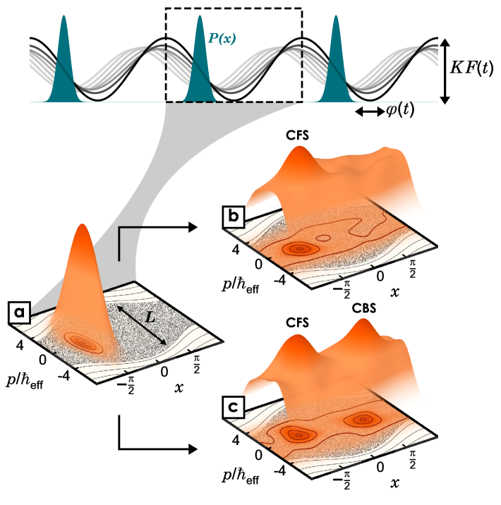
Figure 1: Top: Sketch of the initial atomic density in a 1D lattice, which is subsequently periodically modulated in position ($\varphi(t)$) and amplitude ($F(t)$). Bottom: Experimentally measured Husimi quasi-distributions of (a) the initial squeezed Gaussian state peaked at $x=-\pi/2$, shown above the classical stroboscopic phase portrait, which highlights the classically chaotic region of size $L_{p}=L\hbar_{\mathrm{eff}}$. After undergoing periodic modulation for an evolution time $t>t_{H}$ sufficient for localization to set in, the coherent scattering peaks are measured: (b) In the absence of an appropriate time-reversal symmetry, only the CFS peak is observed. (c) When the dynamics possess the appropriate symmetry, both the CFS and the CBS peak, at $x=\pm\pi/2$ are observed. The Husimi distributions are obtained from a tomographic full quantum state reconstruction, combined for (b,c) with an average over realizations of chaotic dynamics (see text and Appendix for details).

Dynamical chaos [1] has long been a cornerstone in understanding how physical systems governed by deterministic, time-reversal-invariant equations can lead to probabilistic descriptions, which lie at the heart of statistical physics [2]. Chaotic dynamics generally imply ergodicity, a regime in which the time spent in each accessible phase space region is proportional to its volume. Recently, the study of chaotic dynamics and its associated relaxation towards an equilibrium distribution has attracted considerable attention in closed quantum systems, such as ultracold atomic gases, trapped ions, and spin qubits [3, 4]. These systems, exceptionally well-isolated from their environment, provide ideal platforms for exploring the fundamental question of whether a quantum system can relax to a stationary equilibrium, through its own unitary dynamics [5].

Consequently, the mechanisms that allow evading this relaxation, i.e. non-ergodicity, have also been under scrutiny. Anderson localization, arising from the interplay between disorder or chaotic diffusion and interference effects [6, 7, 8, 9], and its recent generalization, many-body localization [10, 11, 12, 13], have been identified as key mechanisms for non-ergodicity. Other mechanisms, particularly in many-body quantum systems, have also been recently highlighted, e.g. quantum many-body scars [14], fragmentation of Hilbert space [15, 16], dynamical symmetries [17], and prethermalization in periodically driven systems [18]. This is also reminiscent of classical systems with mixed dynamics, where phase space contains regular trajectories within a chaotic sea, classical barriers, or inhomogeneous chaotic properties [1, 19].

In ergodic and non-ergodic systems alike, dynamics is affected by symmetries. Even in systems exhibiting fully chaotic classical dynamics, time-reversal symmetry can significantly influence quantum transport. For example, the well-known Coherent Backscattering (CBS) peak disappears without time-reversal symmetry [20, 21, 22]. Spectral statistics of quantum chaotic or disordered systems crucially depend on this symmetry [7, 23, 24]. Additionally, topological effects can induce edge states protected from disorder, representing another non-ergodic behavior [25]. These topological properties typically exist at low temperatures or in the low-energy sector, but are generally destroyed at finite temperatures or energy densities, unless non-ergodicity, such as that induced by many-body localization, prevents thermalization [26].

One important goal is thus to find distinctive signatures allowing to unambiguously detect non-ergodic and ergodic behaviors and the symmetry properties of the system. While imbalance or entanglement entropy growth have been highlighted in the many-body regime [10, 14], another signature of non-ergodicity was recently discovered in the non-interacting Anderson localization context: the Coherent Forward Scattering (CFS) peak [27, 28, 29, 30, 31, 32, 33]. This peak arises from disorder-average-immune interference effects when the quantum dynamics is effectively confined in phase space.

Such confinement, a strong manifestation of non-ergodicity, can be induced by a potential well or classical dynamical barriers, or by interference-induced strong localization effects. In spatially localized systems, it leads to a peak in the forward direction in the final momentum distribution of an initial plane wave propagating through a disordered medium [28]. More generally, it appears in the reciprocal space of the one where localization occurs [30]. This peak emerges only after localization has set in and disappears in the diffusive transport regime [31]. Interestingly, it can also detect highly non-trivial forms of non-ergodic behavior, such as quantum multifractality, which arises at the Anderson transition between localized and delocalized phases [31, 32]. Finally, it crucially depends on the symmetries of the system, either through its contrast or its growth dynamics [33].

Cold-atom platforms, with high degree of control over experimental parameters, have proven particularly fruitful for investigating localization effects, from the direct observation of 1D Anderson localization in a disordered potential [34] to the measurement of the Anderson transition in a kicked-rotor atomic system [35, 36]. Other localization-related phenomena have also been observed, such as enhanced return to the origin [37] and the boomerang effect [38]. Furthermore, in experiments where a carefully chosen quasi-periodic kicking creates an effective synthetic dimension, contributions to the return to initial momentum associated with CBS and CFS could be distinguished [21].

In this Letter, we report the first direct observation of the CFS peak and demonstrate that it is not only a hallmark of non-ergodicity but also encodes the symmetries present in the system. We implement a shaken rotor model, using a Bose-Einstein condensate (BEC) of ultracold atoms in a modulated optical lattice. Like the kicked rotor, it exhibits chaotic classical dynamics and dynamical localization in momentum space in the quantum regime [39], implying coherent scattering peaks in the position distribution. Crucially, the shaken rotor enables to tailor the symmetries of the dynamics, while performing an average over realizations of chaos. Leveraging the high degree of control over our system, we prepare an initially narrow position distribution that subsequently undergoes chaotic dynamics in the modulated lattice. Additionally, we finely tune the characteristics of the modulation to control both the system’s localization scale and the symmetries of its dynamics. This allows us to measure the suppression or enhancement of scattering peaks under various symmetry regimes and to highlight the relation between the localization length and the growth timescale of the CFS.

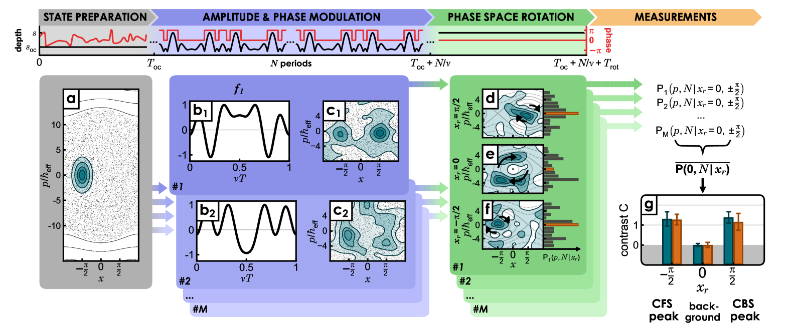
Figure 2: Experimental protocol. First, a highly squeezed Gaussian state centered at $x=-x_{0}=-\pi/2$ is prepared by a tailored lattice position (phase) modulation, using an optimal control (OC) algorithm for a fixed lattice depth $s_{\rm oc}$ and for a time $T_{\rm oc}$. The Husimi distribution of this initial state is represented in a. The lattice depth is subsequently shaken for $N$ time periods with different periodic modulation functions $f_{m}$, $1\leq m\leq M$ (see frames b). The functions have a period $\nu^{-1}$ and contain $N_{H}$ harmonics with variable phases (see text). After modulation (see c), we perform a phase space rotation, holding the state for a quarter of the period in a static lattice of depth $s$. This transfers the probability density at the center of a lattice site onto the zero momentum component, whose population is measured by imaging the atoms after a time-of-flight (see d, e, f). This procedure is performed three times with three centers of rotation $x=x_{r}=-\pi/2,0,\pi/2$, set by a shift of the lattice phase, giving the evolutions and momentum populations $P_{m}(p,N|x_{r})$ represented in panels d, e, f, and the bar diagrams on their right. This experiment is repeated $M$ times with different modulation function $f_{m}$, starting from the same initial state. By averaging all the contributions $P_{1}$,$...$,$P_{M}$ we obtain the signal encoding the CFS and CBS peaks and the background in the average amplitude of the zero momentum component. g Depending on the modulation regime and symmetries, the CBS or/and CFS peaks emerge from the background (blue, left: numerics, orange, right: experiment). The contrast is defined in g with respect to the background measured for $x_{r}=0$ (see text). Error bars indicate one standard deviation of the mean. Parameters: $s=24.2\pm 0.28$, $M=10$, $N_{H}=5$, $\nu=35.05$ kHz and $N=18$.

A matter wave shaken rotor model

Our experiments realize a shaken rotor model:

$$\hat{\mathcal{H}}=\frac{\hat{p}^{2}}{2}-K\cos\left(\hat{x}+\varphi(t)\right)F(t),$$ (1)

where $\hat{x}$ and $\hat{p}$ are the position and momentum operators respectively, with $-i[\hat{x},\hat{p}]=\hbar_{\mathrm{eff}}$ an effective Planck constant. $K$ is the modulation strength, and $\varphi(t)$ and $F(t)$ describe the periodic position and amplitude modulations of the sinusoidal potential, with period 1. The function $F(t)$ sums to 1 over one period of modulation. In the specific case of $\varphi=0$ and $F=\sum_{n}\delta(t-n)$, (1) reduces to the celebrated kicked rotor [1].

As for the kicked rotor, the shaken rotor Hamiltonian (1) induces fully chaotic classical dynamics for large modulation strengths, $K>9$ (see Appendix). In the quantum regime, this chaotic dynamics leads to dynamical localization [1, 23, 39]: the initially diffusive linear increase in momentum variance induced by the shaking is eventually halted through a multiple interference mechanism in momentum space, analogous to Anderson localization [40]. This non-ergodic behavior gives rise to non-ergodic signatures in the reciprocal space of the localization, i.e. in position space [30], which we directly measure for the first time in this work, as illustrated in Figure 1.

An initial spatially periodic wavefunction with a narrow distribution within each cell of the sinusoidal potential, after a few modulation periods under chaotic dynamics, evolves on average into a state with an almost uniform distribution. If dynamics possess the appropriate symmetry, a CBS peak appears at the opposite position on the same short timescale. This peak, often discussed for wave scattering in disordered media, has been observed in many contexts [41, 42, 43, 44, 45, 46, 22]. It crucially depends on time-reversal symmetry $\mathsf{T}$ for wave scattering in spatial disorder. In the case of dynamical localization, the key symmetry for CBS is $\mathsf{PT}$-symmetry, the product of time-reversal and parity symmetries, with the transformations $t\rightarrow-t$, $x\rightarrow-x$, and $p\rightarrow p$ [47, 30]. Over a longer timescale, given by the Heisenberg time $t_{H}$, which scales with the typical size of dynamical localization, a CFS peak appears at the initial position. This peak is known to be a marker of localization properties in the system [31]. The experimentally measured Husimi distributions shown in Figure 1 reveal these characteristic peaks in the position distribution.

The shaken rotor Hamiltonian (1) differs from the kicked rotor in two key aspects. First, the amplitude modulation function is a truncated sum of harmonics:

$$F(t)=1+2\sum_{n=1}^{N_{H}}\cos(2\pi nt+\phi_{n}),$$ (2)

where $N_{H}$ is the number of harmonics, and $\phi_{n}$ their respective phases. This limits the momentum extension $L_{p}$ of the region where classical chaotic dynamics occurs, which is proportional to $(2N_{H}+1)$. In the quantum regime, the other characteristic length is the localization length $\xi_{p}$ for dynamical localization, which scales as $K^{2}$ (see Appendix). The model (1) therefore enables to control the localization regime: for parameters where $L_{p}\gg\xi_{p}$, non-ergodic properties are induced by localization ("localized" regime), while for $L_{p}\ll\xi_{p}$, they correspond to classical confinement within dynamical barriers ("classically bounded" regime). Second, the choice of modulation functions $F$ and $\varphi$ allows us to control the symmetries (such as $\mathsf{T}$ and $\mathsf{PT}$) of the dynamics, leading to enhancement or suppression of the coherent scattering peaks.

Finally, the coherent scattering peaks appear as a statistical effect, requiring averaging over several different classical chaotic dynamics. In this work, the use of a coherent matter wave and tunable modulation functions provides a straightforward averaging method: for a given initial state, localization regime, and symmetries of the dynamics, different modulation functions are available, each leading to different chaotic dynamics (see Appendix). By repeating our experiments with several modulation functions, we can obtain the averaged scattering peaks in the chosen regime. This is in contrast with the average over initial conditions usually performed in previous kicked rotor experiments [39].

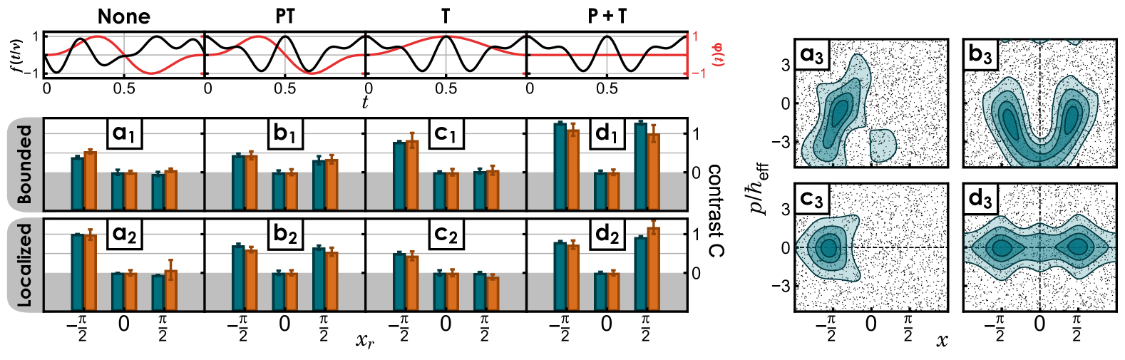
Figure 3: Left (top): Shape of periodic modulations of lattice depth (black) and position (red) corresponding to symmetries (none, $\mathsf{PT}$, $\mathsf{T}$, $\mathsf{P+T}$ for panels a-d respectively). (bottom) Experimental (orange) and numerical (blue) contrasts obtained for different symmetries of the modulation, and in two different localization regimes: bounded $\xi_{\rm loc}/L\gtrsim 1$, and localized $\xi_{\rm loc}/L\lesssim 0.1$, where $\xi_{\rm loc}=\xi_{p}/\hbar_{\mathrm{eff}}$ is the localization length and $L=L_{p}/\hbar_{\mathrm{eff}}$ the extension of the chaotic sea, in units of $\hbar_{\mathrm{eff}}$. The signals are obtained using the method presented in Fig. 2 with an additional average over 3 modulations periods ($N=[15,16,17]$ and $M=10$ if not otherwise stated). ($\mathbf{a_{1}}$) $L=9.24\pm 0.16$, $\xi_{\rm loc}=42\pm 26$, $M=17$, ($\mathbf{a_{2}}$) $L=48.56\pm 0.24$, $\xi_{\rm loc}=4.47\pm 1.43$, $N=[6,7,8]$, ($\mathbf{b_{1}}$) $L=9.90\pm 0.10$, $\xi_{\rm loc}=31\pm 16$, ($\mathbf{b_{2}}$) $L=62.70\pm 0.58$, $\xi_{\rm loc}=1.9\pm 0.73$, ($\mathbf{c_{1}}$) $L=9.04\pm 0.10$, $\xi_{\rm loc}=29.5\pm 16$, ($\mathbf{c_{2}}$) $L=23.96\pm 0.38$, $\xi_{\rm loc}=1.52\pm 0.35$, ($\mathbf{d_{1}}$) $L=8.42\pm 0.32$, $\xi_{\rm loc}=20.1\pm 8.5$, ($\mathbf{d_{2}}$) $L=25.78\pm 0.42$, $\xi_{\rm loc}=0.77\pm 0.05$. Right (a₃-d₃): Husimi distributions of a characteristic Floquet eigenstate (see text for details) in the four regimes of symmetry of the dynamics.

Experimental setup and method

Our experiments start with a BEC of about $5\cdot 10^{5}$ rubidium-87 atoms produced in a hybrid trap (see Appendix) and then placed in a 1D optical lattice potential:

$$V(X,T)=-\frac{s}{2}f(T)E_{L}\cos(2\pi\frac{X}{d}+\varphi(T))$$ (3)

with $d=532\,{\rm nm}$ the lattice spacing, $E_{L}=h^{2}/(2md^{2})=h\nu_{L}$ its energy scale, $h$ the Planck constant and $m$ the atomic mass. The optical lattice is produced by the interference of two far-detuned counter-propagating beams derived from the same laser, whose amplitude and phase are controlled in time by acousto-optic modulators (AOM). We vary the depth $sf(T)$ of the lattice potential, where $|f(T)|\leq 1$ and $s$ is the maximum achievable depth, and its position $\varphi(t)$.

For a periodic modulation of the lattice with frequency $\nu$, we recover the Hamiltonian (1) with dimensionless variables $t=\nu T$, $x=2\pi X/d$, and $p=2\pi P/(md\nu)$, modulation function $f(T)=F(\nu T)/\max(|F|)$ and modulation strength $K=4\pi^{2}s(\nu_{L}/\nu)^{2}/\max(|F|)$. The tunable effective Planck constant is $\hbar_{\mathrm{eff}}=4\pi(\nu_{L}/\nu)$.

A single experimental sequence comprises three steps, sketched in Figure 2. In the first step we prepare the initial quantum state in the lattice: the BEC is adiabatically loaded into the ground state of a static lattice with a moderate depth of $s\times f(T=0)\simeq 5$. In the lattice band structure, this ground state belongs to the subspace of zero quasi-momentum, preserved under modulation. Therefore, the subsequent evolution of the state can be expressed as a superposition of plane waves with discrete momenta $p=\ell\hbar_{\mathrm{eff}}$. Throughout the dynamics, the state can be characterized by a measurement of the average populations in these momentum components, performed by absorption imaging of the BEC released from the trap, after a time-of-flight.

The ground state is then transformed into a periodic state with a squeezed Gaussian position distribution in each lattice site, centered on $x=-x_{0}=-\pi/2$, and of width $\Delta x/(2\pi)\simeq 4\%$ for experiments presented here (see Fig. 2 a). Such a narrow Gaussian distribution cannot be achieved through adiabatic loading, as it would require extraordinary lattice depths ($s\simeq 200$). We therefore perform quantum state preparation with a modulation of the lattice phase $\varphi(T)$ derived from a quantum optimal control algorithm [48]. This state preparation modulation is performed in the initial fixed-depth lattice with $s_{oc}=s\times f\simeq 5$ and allows us to produce the peaked initial state in a typical duration $T_{oc}\simeq 100\,\mu$s, with a high fidelity (see Fig. 1 a, Fig. 2 a and Appendix).

The precise choice and preparation of the initial state are crucial to our measurements. The width of the initial state results from a compromise: a too broad position distribution leads to reduced CFS and CBS contrasts [30], but the initial state has to evolve primarily in the chaotic region, implying a momentum extension smaller than $L_{p}$.

The second and main step performs the chaotic dynamics, through a choice of periodic modulation functions $\{F(t),\varphi(t)\}$ with given symmetries. The amplitude modulation $F(t)$, which is a sum of harmonics, may take negative values, implemented via a sudden $\pi$-shift of the lattice phase $\varphi$ when the lattice amplitude reaches zero (see Figure 2). After a given number $N$ of modulation periods, the system has undergone chaotic dynamics, and is expected to display on average a spreading over the classically chaotic sea, with the coherent scattering peaks superimposed (see Fig. 1).

The final step corresponds to a regular phase space dynamics: the state is held in a static lattice with maximal depth $s$ for a duration close to a quarter-period at the lattice well frequency $T_{\mathrm{rot}}\simeq(\sqrt{s}\nu_{L})^{-1}/4$. This amounts to a $\pi/2$-rotation in phase space around the bottom of the well, transferring the position distribution into momentum space [30]. Specifically, by positioning the expected coherent peaks (in position) at the center of the wells through a sudden position shift $x_{r}=\pm\pi/2$ before the rotation, we convert them into a peak in the momentum distribution $|c_{\ell}|^{2}$ at $p=\hbar_{\mathrm{eff}}\ell=0$ (see Figure 2 d-f). The measured probability $P(p=0,N|x_{r}=\pm\pi/2)$ can then be compared to the value for $x_{r}=0$, which reflects the background.

This final phase space rotation must accurately convert the peak in the position distribution into a peak at momentum $p=0$. This turns out to be the primary limit on the momentum extension of the initial squeezed state. Initial state preparation and phase space rotation parameters were optimized in light of these constraints (see Appendix).

Each choice of modulation functions $\{F(t),\varphi(t)\}$ thus implies at least three full experimental sequences. Moreover, in order to reveal the CBS and CFS peaks, we need an average over disorder, i.e. over different modulation functions with given parameters $(K,\hbar_{\mathrm{eff}})$ and chosen symmetries. For each configuration considered, the data are obtained by averaging over $M=10$ amplitude modulation functions $F(t)$, with a fixed phase modulation $\varphi(t)$ setting the symmetry. The averaged probability $\overline{P(p=0,N|x_{r}=\pm\pi/2)}$ measured near zero momentum after phase space rotation and time-of-flight, compared to the value obtained for $x_{r}=0$, constitutes a direct measurement of the contrast of the CFS and CBS peaks, $\mathsf{C}_{CBS,CFS}=\overline{P(0,N|x_{r}=\pm\pi/2)}/\overline{P(0,N|x_{r}=0)}-1$, as shown in Figure 2 g. Our experimental results are compared to extensive numerical simulations of the dynamics through the time-dependent Schrödinger equation (TDSE - see Appendix).

Results

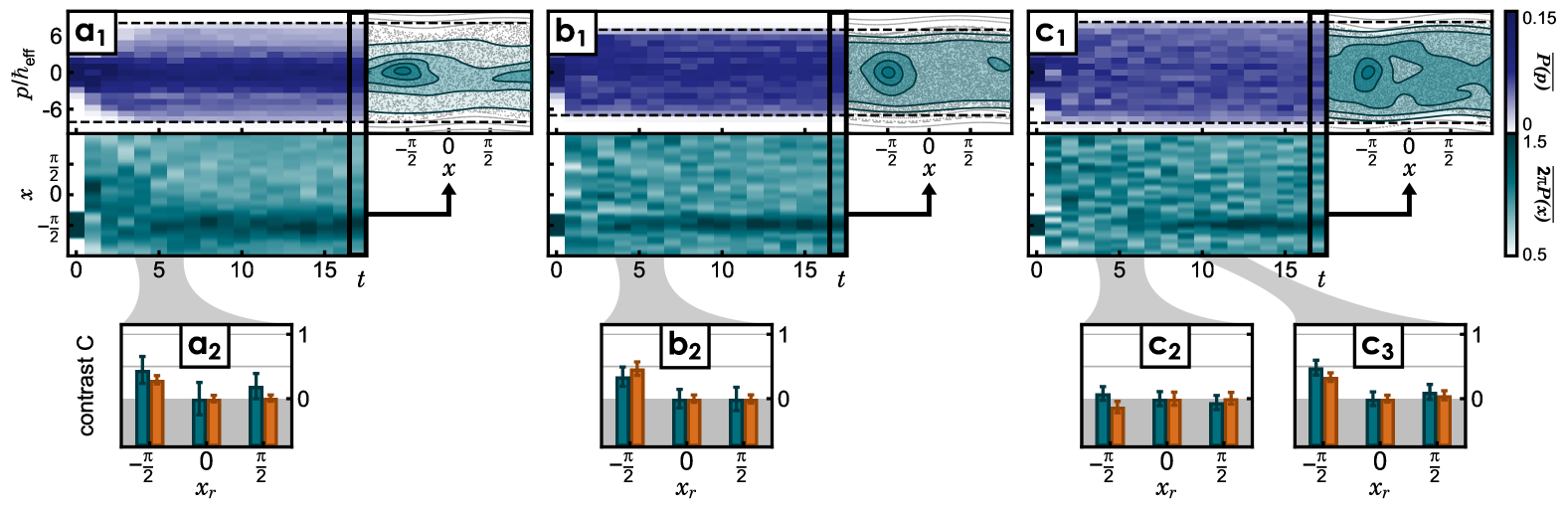
Figure 4: CFS apparition timescale for various localization regimes and chaotic sea sizes $L$. Top panels show the averaged momentum distribution $\overline{P(p)}$ as a function of time, with the Husimi representation of the final state to the right. Bottom panels show the corresponding evolution of the averaged spatial density $\overline{P(x)}$. These numerical results are computed in a localized regime with large chaotic sea bounded by the dashed lines ($\mathbf{a_{1}}$), a classically bounded regime with a “small” chaotic sea ($\mathbf{b_{1}}$) and a bounded regime with a “large” chaotic sea ($\mathbf{c_{1}}$). Experimental and numerical signals (obtained as per Fig. 2) are shown at a short modulation time ($N=[4,5,6]$) for all cases ($\mathbf{a_{2}}$, $\mathbf{b_{2}}$, $\mathbf{c_{2}}$), and at a longer time for the case c ($N=[10,11,12]$, $\mathbf{c_{3}}$), showing the later appearance of the CFS peak. Parameters: (a) $L=15.52\pm 0.34$, $\xi_{\rm loc}=5.97\pm 2.8$, (b) $L=12.8\pm 0.46$, $\xi_{\rm loc}=18.5\pm 7.2$, (c) $L=15.9\pm 0.24$, $\xi_{\rm loc}=52.5\pm 26$.

We have applied our measurement protocol in the localized and classically bounded regimes of the shaken rotor, varying the symmetry regime. The tailoring of symmetries through modulation functions is illustrated in Figure 3 (top row). A key symmetry of interest is $\mathsf{PT}$ symmetry (Fig. 3 b), achieved through a combination of time-symmetric amplitude modulation, $F(1-t)=F(t)$, and anti-symmetric position modulation, $\varphi(1-t)=-\varphi(t)$. Symmetric amplitude and position modulation realize the usual time-reversal $\mathsf{T}$ symmetry (Fig. 3 c), and we can combine both symmetries, with symmetric $F$ and $\varphi=0$, to obtain dynamics that are both $\mathsf{P}$ and $\mathsf{T}$ invariant (Fig. 3 d). The periodic phase modulation is chosen with a minimum number of harmonics while ensuring $\mathrm{d}\varphi/\mathrm{d}t(t=0)=0$, to guarantee a continuous variation of momentum in the lattice. The amplitude modulation $F(t)$ is symmetric for a random choice of $\phi_{n}=0$ or $\pi$ for the phase of each harmonic, while this phase can be chosen randomly between $0$ and $2\pi$ to break the symmetry.

The symmetries of the dynamics are reflected in the structure of the eigenstates of the one-period evolution operator, or Floquet states, as highlighted in Figure 3 $\mathrm{\mathbf{a_{3}-d_{3}}}$, which shows the Husimi distribution of the Floquet state with maximum overlap to the initial peaked state in $x=-x_{0}$, for each symmetry regime. As expected, $\mathsf{PT}$-symmetry reflects in a symmetry of the Floquet states with respect to space inversion $x\rightarrow-x$, while the $\mathsf{T}$-symmetric states are symmetric with respect to momentum inversion $p\rightarrow-p$.

The CBS and CFS contrasts in Figure 3 constitute the main result of this work, and vividly illustrate the impact of both symmetry and localization regimes on these coherent signatures of non-ergodicity. In all regimes (Fig. 3 a-d) a CFS peak is present, demonstrating that it is a robust marker of non-ergodicity, be it from dynamical localization over a length $\xi_{loc}=\xi_{p}/\hbar_{\mathrm{eff}}$ (in units of $\hbar_{\mathrm{eff}}$), or box-constrained dynamics (with extension $L=L_{p}/\hbar_{\mathrm{eff}}$). The CBS peak, which relies on the interference of symmetric trajectories, is only observed when the appropriate $\mathsf{PT}$ symmetry is present (Fig. 3 b and d), where it mirrors the CFS peak.

We also observe the enhancement of the CFS when $\mathsf{T}$-symmetry is present, in the bounded regime (Fig. 3 $\mathrm{\mathbf{c_{1}}}$). This can be understood as a form of enhanced return to the origin, which occurs for the kicked rotor in momentum space in the presence of $\mathsf{PT}$-symmetry [37, 21], but arises here in position space due to $\mathsf{T}$-symmetry: chaotic trajectories originating from and returning to the original position interfere constructively with time-reversed counterparts, increasing the return probability. In the localized regime where $L\gg\xi$, this enhancement is blurred by the finite width $\Delta x\gtrsim 1/L$ of the initial state [30]. The addition of $\mathsf{T}$-symmetry in this regime does not lead to a measurable increase of the CFS contrast (Fig. 3 $\mathrm{\mathbf{c_{2}}}$).

Combining both symmetries, we recover the CBS peak alongside the CFS peak ($\mathsf{PT}-$symmetry), with an additional enhancement of both CBS and CFS contrasts in the bounded regime due to $\mathsf{T}-$symmetry. The measurements in Figure 3 show good agreement with TDSE simulations, with variations in the observed CBS and CFS contrasts well reproduced by numerical results.

The tomographic approach from which we extract the signal of the coherent scattering peaks of Figure 3 can be extended to perform full state characterization [49]. By modifying the final step in Figure 2, we can instead record the momentum distribution for several holding times in the static lattice of depth $s$. This dynamical evolution provides a complete tomography of the final state of the system, from which we can obtain a maximum likelihood state estimate, $\hat{\rho}_{ML}$ (see Appendix). With this state estimate, the phase space Husimi quasi-probability distribution can be readily computed. This was done for the initial state shown in Figure 1 a. For the final states, averaging state reconstruction results over the $M$ modulation functions provides a disorder-averaged state estimate, and the phase space distributions shown in Fig. 1 b,c reveal the coherent scattering peaks.

Finally, we experimentally demonstrate that the CFS is a quantitative marker of non-ergodicity, by investigating its growth dynamics, shown in Figure 4. The typical timescale $t_{H}$ for appearance of the CFS is that of localization, either from dynamical localization ($t_{H}\sim\xi_{loc}$) or from the bounded chaotic dynamics ($t_{H}\sim L$). We can highlight this link by tuning both $\xi_{loc}$ and $L$. In all data of Figure 4, no symmetry is present, and only the CFS is expected. In Figs. 4 $\mathrm{\mathbf{a_{2}}}$ and $\mathrm{\mathbf{b_{2}}}$, the CFS is clearly visible in measurements after approximately 5 periods of modulation. This non-ergodic signature is, however, of two distinct origins, (exponential) dynamical localization with $\xi^{(a)}_{loc}\ll L^{(a)}$, or bounded diffusion within a limited-size box $L^{(b)}$, as illustrated by numerically computed evolutions (Fig. 4 $\mathrm{\mathbf{a_{1}}}$ and $\mathrm{\mathbf{b_{1}}}$). In Fig. 4 c, modulation parameters are chosen such that the dynamics is also essentially a bounded diffusion within a chaotic sea of size $L^{(c)}\simeq L^{(a)}>L^{(b)}$. The growth of the CFS is delayed, as expected, compared to the other measurements, and it becomes visible after about 11 periods of modulation. This manifests the critical interplay between the characteristic sizes $\xi_{\mathrm{loc}}$ and $L$ in setting the CFS dynamics, which conversely establishes the CFS dynamics as a quantitative marker of the non-ergodic properties of the system.

Discussion

We have demonstrated a new method for the investigation of non-ergodicity using cold atoms in a shaken rotor potential. Critically, our system allows for a genuine average over chaotic dynamics, while retaining control over the effective system size, localization length and symmetries of the dynamics. With this method, we have realized the first direct measurement of the CFS peak, appearing in position space in our system. Varying the symmetry regimes, we highlight their role in the appearance of a CBS peak, as well as the enhancement of both scattering peaks. The CFS stands out as a hallmark of non-ergodicity, and we measure its dependence on the controllable characteristic lengths establishing it as a quantitative marker of localization properties.

The time-dependent growth of the CFS peak notably encodes the spectral form factor —a key quantity challenging to measure experimentally—and reveals key symmetries (J. Hebraud et al., in preparation). Our results open new avenues for exploring quantum many-body chaos and localization through the coherent signatures of non-ergodicity.

Acknowledgements

We are grateful to the late D. Delande for many insightful and enriching discussions. We thank Calcul en Midi-Pyrénées (CALMIP) for computational resources. This work was supported by the ANR projects QuCoBEC (ANR-22-CE47-0008) Gladys (ANR-19-CE30-0013), QUTISYM (ANR-23-PETQ-0002) and ManyBodyNet, the EUR Grant NanoX No. ANR-17-EURE-0009, by the Singapore Ministry of Education Academic Research Funds Tier II (WBS No. A-8001527- 02-00 and A-8002396-00-00) and the ERC Grant LATIS.

Appendix

Experimental setup

Our experimental setup produces Bose-Einstein condensates (BEC) of rubidium-87 in a hybrid (magnetic and dipolar) trap, with weak harmonic trapping (angular frequencies ($\Omega_{x},\Omega_{y},\Omega_{z}$)=$2\pi\times({7,73,66})\,{\rm Hz}$) [48]. This confinement does not affect the dynamics over the timescale of the experiments. A 1D optical lattice with spatial period $d=532$ nm is superimposed to the hybrid trap on the $x$-axis. The optical lattice is produced by the interference of two far-detuned counter-propagating beams derived from the same laser. An acousto-optic modulator (AOM) controls the laser amplitude, while two other phase-locked AOMs placed on each lattice beam control their relative phase. The lattice depth $s$ and phase $\varphi$ can thus be arbitrarily and independently time-modulated. The bandwidth for amplitude or phase modulation is about $1\,\mathrm{MHz}$. The Hamiltonian describing the dynamics in the lattice writes

$$\hat{H}=\frac{\hat{P}^{2}}{2m}-\frac{sE_{L}}{2}\cos\left(k_{L}\hat{X}+\varphi(T)\right)f(T),$$ (A1)

with $m$ the atomic mass, $k_{L}=2\pi/d$ the lattice wavevector and $E_{L}=\hbar^{2}k_{L}^{2}/2m=h\nu_{L}$ the lattice characteristic energy, with the characteristic lattice frequency $\nu_{L}$. The maximum reachable lattice depth is $s\leq 40$.

System modeling

To model the experimental wavefunction, which occupies a finite number of lattice sites, it is written as a superposition

$$\Psi(x,t)=\int_{-0.5}^{0.5}\mathrm{d}\beta\Phi(\beta)\Psi_{\beta}(x,t),$$ (A2)

where $\absolutevalue{\Phi(\beta)}^{2}$ is a narrow quasi-momentum distribution centered on $\beta=0$ with $\int_{-0.5}^{0.5}\absolutevalue{\Phi(\beta)}^{2}\mathrm{d}\beta=1$, and the components $\Psi_{\beta}(x,t)$ are normalized wavefunctions evolving in the subspace of quasi-momentum $\beta$, which can be decomposed on a set of plane waves:

$$\Psi_{\beta}(x,t)=\sum_{\ell}c_{\ell,\beta}(t)\frac{1}{\sqrt{2\pi}}e^{i(\ell+\beta)x}.$$ (A3)

The planewave $\ket{\ell+\beta}$ is an eigenstate of momentum with eigenvalue $p=\left(\ell+\beta\right)\hbar_{\mathrm{eff}}$ and wavefunction $\innerproduct{x}{\ell+\beta}=\frac{1}{\sqrt{2\pi}}e^{i(\ell+\beta)x}$.

Experimentally, we measure the momentum population after a time-of-flight. This measurement does not resolve quasi-momentum components and provides the momentum density averaged over quasi-momenta near integer multiples of $\hbar_{\mathrm{eff}}$, $P(p\simeq\ell\hbar_{\mathrm{eff}},t)=\int\mathrm{d}\beta|\Phi(\beta)|^{2}|c_{\ell,\beta}(t)|^{2}$. Since we measure an average of all lattice sites contributions, the corresponding spatial density is the one-site density averaged over all sites, $P(x,t)$.

The average across multiple experiments is done by taking a statistical average for both densities over the evolution obtained from several modulation functions.

Modeling $\absolutevalue{\Phi(\beta)}^{2}$ as a rectangular distribution centered at $\beta_{m}=0$ with a width of $\Delta\beta=0.1$ gives good agreement with experiments. This distribution is discretized over a number of quasi-momenta, $N_{\beta}$, which depends on the simulation and is chosen to ensure that no boundary effects arise from the dynamics in position space. Typically $N_{\beta}=51$.

Simulations use a discretization of the evolution operator from the time-dependent Schrödinger equation (TDSE), $\hat{U}(t,0)=\hat{U}(t,t-\delta t)...\hat{U}(\delta t,0)$. The modulation is considered piecewise-constant, with a fixed value during a time step $\delta t$. The typical number of time-steps is $500$ per period. The size of the Hilbert space chosen for computation is also adapted to the dynamics to avoid any boundary effects.

Characteristic lengths: $L$ and $\xi_{\mathrm{loc}}$

In a 1D disordered system, localization of a wave-packet occurs and results in a freezing of the diffusion. In our system this diffusion takes place in momentum space where the localized average density can be approximated as $P(p)=Ae^{-|p|/\xi_{\mathrm{p}}}$. Two characteristic lengths can be measured : the localization length $\xi_{p}$, defined as the scale of the exponential decay of the wavefunction in the absence of a boundary, and the momentum extension of the chaotic sea $L_{p}$, defining the extent in momentum of the area accessible through diffusion. These values can also be expressed in $\hbar_{\mathrm{eff}}$ units : $L=L_{p}/\hbar_{\mathrm{eff}}$ and $\xi_{loc}=\xi_{p}/\hbar_{\mathrm{eff}}$.

These parameters are determined numerically. The chaotic dynamics starting from an initial momentum state $\ket{p=0}$ is simulated, with a lattice modulated by a function $f_{m}(t)$ ($1\leq m\leq M$) and a stochastic parameter $K_{m}>9$. The localization length $\xi_{\mathrm{loc},m}$ is estimated by fitting and taking the mean value from the right and left slopes of the average logarithmic momentum density $\ln(P(p))$ obtained from multiple periods once localization has set in. In most of the results, the average is taken over $70$ periods and starts after period $30$.

The measurement method used in this paper requires multiple modulation functions, each one having a different stochastic coefficient and leading to a different localization length. The estimation of an overall averaged localization length $\xi_{\mathrm{loc}}$ is given by taking the mean value of all $\xi_{\mathrm{loc},m}$. We also define a mean stochastic coefficient $K$.

The momentum extension of the chaotic sea, $L$, is also deduced from the same computation. It is defined as the interval between the left and right sharp drops of the momentum log-density average $\overline{\ln(P(p))}$ over all modulation functions, that correspond to the classical boundaries of the chaotic sea. The values obtained correspond well to the extent of the chaotic sea of the classical phase space.

An example of the determination of $\xi_{\mathrm{loc}}$ and $L$ is given in Figure A1, and all experimental parameters corresponding to the characteristic lengths $L$ and $\xi_{\mathrm{loc}}$ mentioned in Figures 3 and 4 of the main text are referenced in Table A1 along with the average stochastic parameter $K$.

	$\mathit{s}$	$\mathbf{\nu}$	$\mathbf{N_{H}}$	$\mathbf{A_{\varphi}}$	$\mathbf{K}$	$\hbar_{\mathrm{eff}}$
Fig.3 $\mathbf{a_{1}}$	$27.4\pm 0.28$	$10.508$kHz	4	$2$	$125\pm 12$	$9.7$
Fig.3 $\mathbf{b_{1}}$	$27.9\pm 0.38$	$10.454$kHz	4	$2$	$122\pm 8$	$9.75$
Fig.3 $\mathbf{c_{1}}$	$26.1\pm 0.63$	$10.729$ kHz	4	$1$	$110\pm 7$	$9.5$
Fig.3 $\mathbf{d_{1}}$	$26.5\pm 0.1$	$10.673$ kHz	4	$-$	$113\pm 7$	$9.55$
Fig.3 $\mathbf{a_{2}}$	$28.7\pm 0.45$	$12.741$kHz	27	$2$	$20.3\pm 1.4$	$8$
Fig.3 $\mathbf{b_{2}}$	$23.9\pm 0.25$	$26.823$kHz	17	$2$	$9.0\pm 0.1$	$3.8$
Fig.3 $\mathbf{c_{2}}$	$6.3\pm 0.13$	$12.430$kHz	15	$1.5$	$10.9\pm 0.2$	$8.2$
	$s_{rot}=26.8\pm 0.3$
Fig.3 $\mathbf{d_{2}}$	$5.2\pm 0.14$	$10.618$kHz	20	$-$	$11.2\pm 0.1$	$9.6$
	$s_{rot}=22.3\pm 0.4$
Fig.4 $\mathbf{a}$	$11.3\pm 0.18$	$7.078$KHz	15	$4$	$43.3\pm 5.4$	$14.4$
Fig.4 $\mathbf{b}$	$26.3\pm 0.29$	$5.926$KHz	13	$2$	$170\pm 15$	$17.2$
Fig.4 $\mathbf{c}$	$33.9\pm 0.32$	$10.193$kHz	9	$2$	$101\pm 10$	$10$
Fig.A8 $\mathbf{a}$	$19.7\pm 0.21$	$30.888$kHz	5	$1$	$8.76\pm 0.74$	$3.3$

Table A1: Experimental parameters corresponding to the results presented in Figures 3 and 4. The error bars represent one standard deviation across all averaged experiments. $A_{\varphi}$ is the amplitude of additional lattice phase modulation $\varphi(t)$. Specific values of the lattice depth for the phase space rotation $s_{rot}$ are indicated, when it differs from $s$.

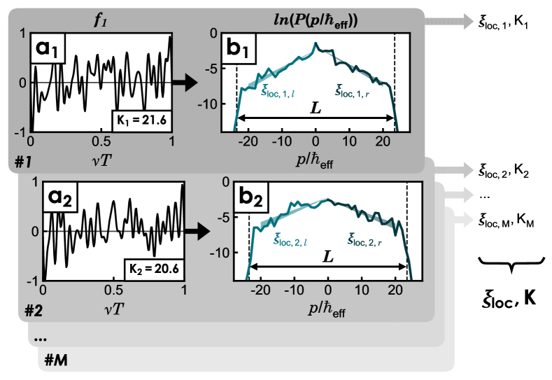
Figure A1: Estimation of the mean localization length $\xi_{\mathrm{loc}}$ and stochastic coefficient $K$. Frames a show the modulation functions and their stochastic coefficients $K_{m}$, and b the corresponding time-averaged momentum density from period 30 to 100 where linear fits on the two slopes give left $\xi_{\mathrm{loc},m,l}$ and right $\xi_{\mathrm{loc},m,r}$ localization lengths. Taking the mean values give $\xi_{\mathrm{loc}}$ and $K$. Parameters: case $\mathbf{a_{2}}$ from Figure 3 of the main text, see table A1.

Initial state preparation using Optimal Control

Measurements of the CBS and CFS peaks in the shaken rotor require a peaked initial state at $x\neq 0$. The phase space rotation measurement also requires a finite momentum extension, contained within the closed trajectories of the static sine-potential phase space. Such a state can be defined using the lattice squeezed Gaussian state

$$\ket{\tilde{G}_{\beta}(x_{c},p_{c},s,\sigma)}=\sum_{\ell\in\mathbb{Z}}c_{\ell,\beta}(x_{c},p_{c},s,\sigma)\ket{\ell+\beta},$$ (A4)

with coefficients

$$c_{\ell,\beta}(x_{c},p_{c},s,\sigma)=\frac{2\sigma^{2}}{\pi\sqrt{s}}e^{ix_{c}p_{c}/2}e^{-i(\ell+\beta)x_{c}}e^{-\sigma^{2}(\ell+\beta-p_{c})^{2}/\sqrt{s}},$$ (A5)

where $\beta$ is the quasi-momentum, $x_{c}$ and $p_{c}$ the Gaussian state average position and momentum in a lattice well, $s$ the lattice depth, and $\sigma$ the squeezing factor quantifying the Gaussian spatial extension $\Delta x=\sigma\Delta x_{0}$ with $\Delta x_{0}=k_{L}^{-1}s^{-1/4}$ the non-squeezed extension, similar to the extension of the ground-state at depth $s$.

We choose $\ket{\Psi_{i}}=\ket{\tilde{G}_{0}(-\pi/2,0,s,0.6)}$ as our initial state, with $s$ the depth used during the phase space rotation. It corresponds to an extension in dimensionless position units of $\Delta x=0.27$ for $s=25$, corresponding to the ground-state width in a lattice with effective depth $s_{\mathrm{eff}}\sim 193$ [49].

This state is prepared through optimal control: starting from a state $\ket{\Psi_{0}}$, a desired target state $\ket{\Psi_{T}}$ can be reached using a lattice phase modulation $\varphi_{\mathrm{oc}}(t)$ determined by a quantum Optimal Control (OC) algorithm [48], which uses gradient ascent to maximize the fidelity to the target $F=|\innerproduct{\Psi_{0}}{\Psi_{T}}|^{2}$. For all our experiments, $\ket{\Psi_{0}}$ is the ground-state of the lattice at depth $s_{\mathrm{oc}}=5$, and the target is a squeezed Gaussian state $\ket{\Psi_{T}}=\ket{\tilde{G}_{0}(0,0,s,0.6)}$ centered in phase space. The OC preparation is determined at depth $s_{\mathrm{oc}}$ for a duration close to $100\,\mu s$ and numerical fidelity $F\geq 0.99$ in subspace $\beta=0$. After the preparation, the lattice phase is shifted with $\pi/2$ to place the Gaussian at $x=-x_{0}=-\pi/2$ to reach the desired initial state $\ket{\Psi_{i}}$.

Quantum state reconstruction

The final experimental state can be characterized using a maximum likelihood reconstruction algorithm to determine its density matrix [49]. The algorithm uses dynamics of the state in a static lattice to iteratively transform an initial-guess density matrix $\hat{\rho}_{0}$ until it converges to the most likely one, $\hat{\rho}_{ML}$.

The likelihood function is defined with respect to the system’s density matrix as:

$$\mathcal{L}\left[\hat{\rho}\right]=\prod_{\ell,\tau}p_{\ell}(\tau)^{f_{\ell}(\tau)},$$ (A6)

with $p_{\ell}(\tau)$ the expected populations of momentum $\ell$ at time $\tau$, as obtained from $\hat{\rho}$, raised to the power of $f_{\ell}(\tau)$, the corresponding experimentally measured populations. The likelihood reaches its maximum when the probabilities from $\hat{\rho}$ match the measurements.

The maximum likelihood algorithm introduces the operator in the zero quasi-momentum subspace

$$\hat{R}\left[\hat{\rho}\right]=\sum_{\ell,\tau}\frac{f_{\ell}(\tau)}{p_{\ell}(\tau)}\hat{\varepsilon}_{\ell}(\tau),$$ (A7)

with $\hat{\varepsilon}_{\ell}(\tau)=(1/N_{\tau})\hat{U}^{\dagger}(\tau,0)\ket{\ell}\bra{\ell}\hat{U}(\tau,0)$ forming a positive operator-valued measure (POVM). Repeated application of $\hat{R}$ to the initial guess iteratively increase the likelihood, until a fixed point $\hat{\rho}_{ML}$ is reached, that maximizes the likelihood.

To achieve this experimentally, the procedure is almost the same as the phase space method presented in the main text. After the chaotic dynamics, all modulations are turned off, and the state dynamics is probed in a static lattice ($\varphi=0$ at given depth $s$) with a constant time-step of $2\,\mathrm{\mu s}$ for a total of $N_{t}=21$ steps. This protocol is depicted in Figure A2.

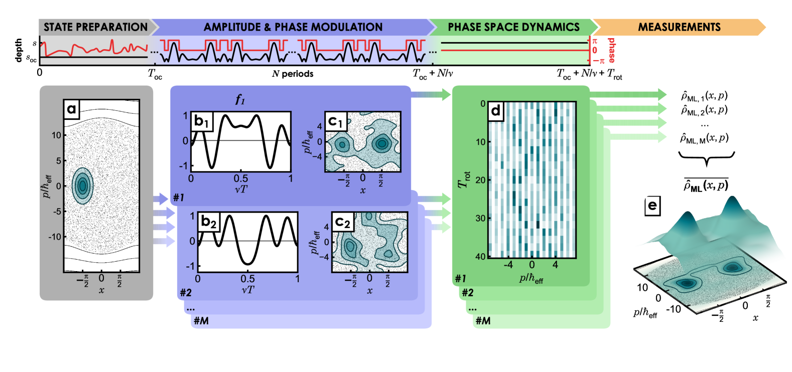
Figure A2: Adapted experimental protocol for reconstruction. Adapted from Figure 2. The preparation and modulation remain unchanged. After modulation, the state evolution is probed in a static lattice of depth $s$ (with no phase shift, $\varphi=0$) over a duration of $40\,\mu$s with steps of $2\,\mu$s. The associated density matrix $\hat{\mathit{\rho}}_{ML,m}$ are reconstructed using a maximum likelihood algorithm [49]. The final density matrix is obtained by averaging over all modulation functions. The average Husimi distribution $\overline{\hat{\mathit{\rho}}_{ML}}$ shown in $\mathbf{e}$ exhibits both CBS and CFS peaks.

Averaged Husimi distribution

Once the density matrix is determined, its Husimi representation is deduced using

$$H_{\hat{\rho}}(x,p)=\frac{1}{2\pi}\langle\tilde{G}_{0}(x,p,s,1)|\hat{\rho}_{ML}|\tilde{G}_{0}(x,p,s,1)\rangle$$ (A8)

which is a projection on a periodic Gaussian state with $\beta=0$ centered on $x$ and $p$.

In this work, the interesting results emerge from averaged signals over different modulation functions. The corresponding Husimi distribution is experimentally obtained by repeating the reconstruction process for each different modulation function, and averaging all associated Husimi distributions. The final mean Husimi can be represented on the phase space of a lattice cell, and reflects the average distribution over the lattice.

In the numerical modeling, the computed Husimi distribution corresponds to the average distribution over a lattice site, and is found by averaging together the Husimi distributions obtained from each considered quasi-momentum component.

Phase space rotation

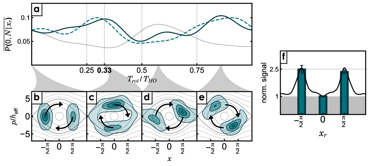
Figure A3: Phase space rotation measurement. After the modulation stage, the state is held in a static lattice and undergoes a phase space rotation. a. The post-rotation signal, defined as the measured average population in momentum 0, is shown for rotation centers $x_{r}=-\pi/2$ (continous line), $x_{r}=\pi/2$ (dashed line) and $x_{r}=0$ (dotted line). b-e. Husimi distribution at different rotation times for $x_{r}=0$ : at $33\%$ of the harmonic oscillator period $T_{HO}$, the two-peaked spatial distribution is mapped into the momentum one. The optimal rotation time is determined as the shortest one maximizing the averaged population in momentum 0 for CBS and/or CFS. f. A normalized post-rotation signal is defined as the measured average population in momentum 0 for $x_{r}=\pm\pi/2$ (associated to CFS or CBS) over that for $x_{r}=0$. Error bars correspond to one standard deviation of the mean.

The phase space rotation measurement relies on a harmonic approximation of a lattice well at large depth $s$ and consists of three phase space rotations of angle $\simeq\pi/2$, centered at positions $x_{r}=-x_{0}=-\pi/2$, $x_{r}=x_{0}$ or intermediate position $x_{r}=0$, to respectively probe CFS, CBS and background.

The evolution of a state peaked at the center of the harmonic oscillator potential during a quarter of its period $T_{HO}=1/(\sqrt{s}\nu_{L})$ converts the position distribution into the momentum distribution. In the finite-depth, anharmonic lattice well, this mapping requires a rotation duration which is not exactly equal to a quarter of $T_{HO}$, and depends on the depth $s$ and the considered state.

The optimized rotation time is numerically determined for each measurement. This optimal time corresponds to the one that maximizes the population $\overline{P(p=0)}$ obtained for $x_{r}=-\pi/2$, averaged over three consecutive modulation periods and over the modulation functions. When CBS is present in the system, the rotation time is taken as the mean between the optimal ones for CFS and CBS. An illustration of this optimization is provided in Figure A3. The obtained signal reflects well the expected peak heights at infinite time in position space [30] (see Fig. A3 f).

Experimentally, to ensure the reproducibility of our data against experimental fluctuations, the populations corresponding to each rotation are measured twice. The absolute difference between the distributions of a pair is computed and compared to a numerical threshold, above which the pair is discarded. This leads on average to the conservation of between 75% and 100% of the data for each parameter set.

Studied symmetries

The Hamiltonian from equation (1) in the main text is an adapted kicked rotor model, in which we have additional control using the amplitude modulation function $F(t)$ and the lattice phase $\varphi(t)$. Both are used to control our system symmetries.

The time-reversal symmetry ($\mathsf{T}$) is easily broken by choosing the harmonics phases $\phi_{n}\in\left[0,\pi\right]$ with at least one of them not zero or $\pi$, implying that $F(t)\neq F(1-t)$. The $\mathsf{T}$-symmetry holds when $F(t)=F(1-t)$, meaning that all $\phi_{n}\in\left\{0,\pi\right\}$.
The parity symmetry ($\mathsf{P}$) is broken when a lattice phase modulation $\varphi(t)$ is used. To reach a desired symmetry, the phase modulation function can be chosen even, $\varphi(t)=A_{\varphi}\left(1-\cos(2\pi t)\right)/2$, or odd $\varphi(t)=2A_{\varphi}/(3\sqrt{3})\left(\sin(2\pi t)-\sin(4\pi t)/2\right)$, with $A_{\varphi}$ a phase modulation amplitude. These phase modulations are chosen to contain a minimum number of harmonics while ensuring a null derivative at $t=0$ in order to guarantee a continuous variation of momentum in the lattice. All tested symmetries are referenced in Table A2.

None	$\mathsf{PT}$	$\mathsf{T}$	$\mathsf{P+T}$
$t\rightarrow t$	$t\rightarrow-t$	$t\rightarrow-t$	$t\rightarrow-t$
$p\rightarrow p$	$p\rightarrow p$	$p\rightarrow-p$	$p\rightarrow-p$
$x\rightarrow x$	$x\rightarrow-x$	$x\rightarrow x$	$x\rightarrow-x$
$F(t)\neq F(1-t)$	$F(t)=F(1-t)$	$F(t)=F(1-t)$	$F(t)=F(1-t)$
$\varphi(t)=-\varphi(-t)$	$\varphi(t)=-\varphi(-t)$	$\varphi(t)=\varphi(-t)$	$\varphi(t)=0$

Table A2: All studied symmetries. The first row lists the symmetry names, the second row their corresponding $x$, $p$ and $t$ transformations, and the last row details the corresponding choice for time-reversibility of the modulation function $F(t)$ and the parity of additional lattice phase modulation $\varphi(t)$.

Comparison between the shaken rotor and the kicked rotor

In this section, we numerically study the properties of classical chaotic diffusion and quantum dynamical localization in the kicked rotor and the shaken rotor. We consider two shaken rotor models: one without symmetry, where the modulation functions are asymmetric in time, and one with $\mathsf{PT}$ symmetry, where the amplitude modulation is time-symmetric and the phase modulation is time-antisymmetric (see Table A2).

.0.1 Classical dynamics

In the kicked rotor, for sufficiently large kicking strength $K\gtrsim 0.97$, classical chaotic trajectories are not confined by regular structures in phase space [50] and ergodically explore the entire chaotic region. This results, on average, in diffusive transport in momentum space [51, 1]:

$$\langle p^{2}(t)\rangle\approx 2D_{cl}t,$$ (A9)

where the average $\langle...\rangle$ is taken over initial conditions with $p=0$ and $x$ randomly sampled in $[0,2\pi]$.

For the shaken rotor, the smooth modulation introduces a crucial difference. The Dirac comb of the kicked rotor’s temporal forcing is replaced by a modulation function $F(t)$ containing only a finite number of frequencies $N_{H}$. As a result, regular trajectories enclose a chaotic sea of finite extent in momentum space, approximately $L_{p}\approx 2\pi(2N_{H}+1)$ (with an actual size also dependent on $K$), see e.g. [52]. Consequently, in the shaken rotor, the classical diffusive transport described by Eq. (A9) persists only for a finite duration before $\langle p^{2}(t)\rangle$ saturates at a finite value.

This is illustrated in Fig. A4 a, where the kicked rotor with $K=40$ exhibits unbounded diffusive transport in momentum space, while for the shaken rotor, $\langle p^{2}(t)\rangle$ saturates at long times to $\langle p^{2}\rangle_{\text{lim}}\approx L_{p}^{2}/12$, corresponding to a uniform distribution over the finite chaotic sea. The classical diffusion coefficient $D_{cl}$, extracted at short times by fitting Eq. (A9) to numerical data, exhibits similar dependence on $K$ in both models, as shown in Fig. A4 b.

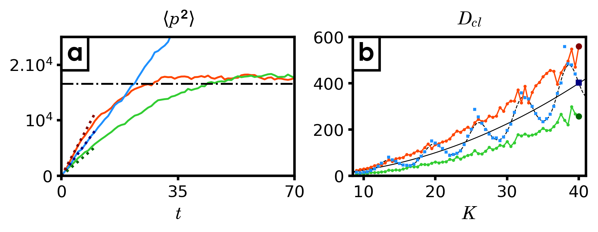
Figure A4: Classical dynamics in the kicked rotor and shaken rotor models. (a) The classical diffusive transport in momentum space for the kicked rotor with large kicking strength $K=40$ follows Eq. (A9), as shown by the blue curve. In the shaken rotor with $K=40$ and $N_{H}=35$, corresponding to a chaotic sea of finite size $L_{p}\approx 446$, diffusion saturates at large times to $\langle p^{2}\rangle_{\text{lim}}\approx L_{p}^{2}/12$ (dashed-dotted horizontal line, see text). The case in the $\mathsf{PT}$-symmetry class is shown in green, while the case in the $\varnothing$-symmetry class is in red. Data are averaged over 1000 initial conditions $\{x_{0},p_{0}=0\}$, with $x_{0}$ uniformly distributed in $[0,2\pi]$, and for the shaken rotor, over 100 different modulation functions. Dotted colored lines indicate linear fits at short times ($t<10$) using Eq. (A9) to extract the classical diffusion coefficient $D_{cl}$, whose values are shown in panel (b). (b) Classical diffusion coefficient $D_{cl}$ versus $K$ in the three models. For the kicked rotor (blue symbols), $D_{cl}$ follows the analytical expression $D_{cl}\approx\frac{K^{2}}{4}\left(1-2J_{2}(K)+2J_{2}(K)^{2}\right)$ (black dashed line, see  [53]), where $J_{2}$ is the ordinary Bessel function of the second order. In the shaken rotor, averaging over different modulation functions suppresses this oscillatory behavior, leading to a scaling $D_{cl}\propto K^{2}$. The black line represents $D_{cl}=K^{2}/4$ for both the shaken rotor in the $\mathsf{PT}$-symmetry class (green symbols) and in the $\varnothing$-symmetry class (red symbols).

.0.2 Quantum dynamical localization

In the quantum regime, the evolution of a wave packet initially peaked at $p=0$ resembles classical diffusion only at short times. At longer times, dynamical localization in momentum space sets in [40, 39]: the wave packet stabilizes into a stationary, exponentially localized distribution characterized by a localization length $\xi_{p}$ in momentum space. Consequently, the variance of the wave packet saturates at $\langle p^{2}\rangle\approx 2\xi_{p}^{2}$. The same phenomenon occurs in the shaken rotor in the limit $L_{p}\gg\xi_{p}$.

Since the two shaken rotor models belong to different symmetry classes, their localization lengths are expected to differ [54, 55]. The $\mathsf{PT}$-symmetry-preserving shaken rotor belongs to the Orthogonal class, while the $\varnothing$-symmetry rotor belongs to the Unitary class. Denoting the localization lengths as $\xi_{p}^{O}$ (Orthogonal) and $\xi_{p}^{U}$ (Unitary), one expects the relation $\xi_{p}^{U}\approx 2\xi_{p}^{O}$ [54, 55]. As a result, the saturation values of $\langle p^{2}\rangle$ differ between the two systems, as seen in Fig. A5 a.

The localization length can be extracted by fitting the exponential decay of the momentum distribution after an evolution time exceeding the localization time, as shown in Fig. A5 b. As expected, the ratio of localization lengths in the two shaken rotor systems is approximately 2 (see Fig. A5 c).

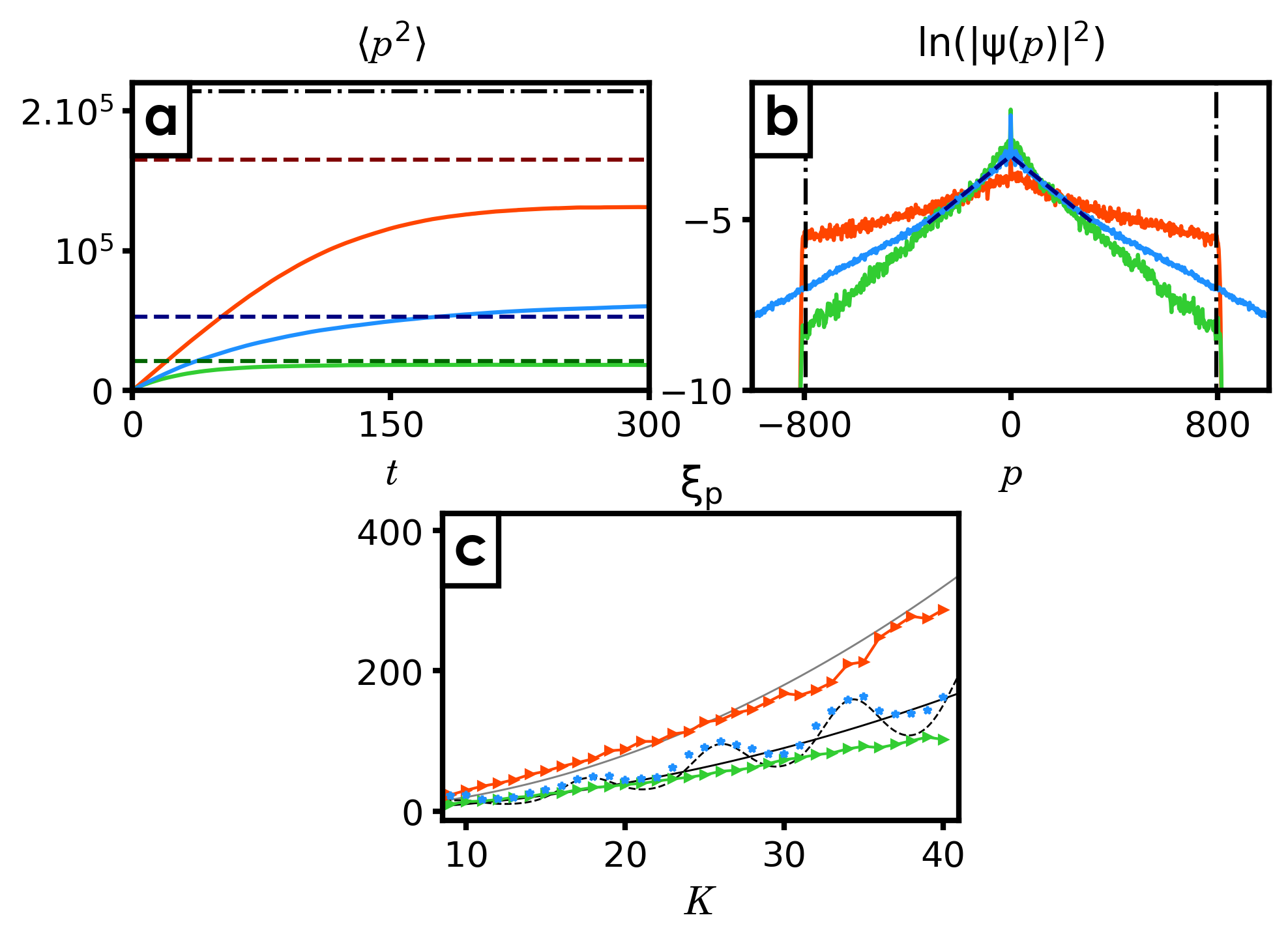
Figure A5: Quantum dynamical localization in the kicked rotor and shaken rotor models. (a) Variance $\langle p^{2}\rangle$ of a wave packet initially peaked at $p=0$ as a function of time in the $\varnothing$-symmetric shaken rotor (red), the $\mathsf{PT}$-symmetric shaken rotor (green), and the kicked rotor (blue). The parameters used are $K=40$, $\hbar_{\mathrm{eff}}=2.5$, and $N_{H}=126$, leading to $L_{p}\approx 2\pi(2N_{H}+1)\approx 1589$ for the shaken rotors. The black dash-dotted line represents the value $\langle p^{2}\rangle=L_{p}^{2}/12$, corresponding to a uniform momentum distribution over the finite chaotic sea. For all three systems with these parameters, the saturation of $\langle p^{2}\rangle$ at large times is due to dynamical localization, with $\langle p^{2}\rangle\approx 2\xi_{p}^{2}$, as indicated by the corresponding colored dashed lines. The values of $\xi_{p}$ are extracted from a fit to the exponential decay of the probability density, as shown in (b). (b) Long-time probability density in momentum space for the three systems, with parameters $K=40$, $\hbar_{\mathrm{eff}}=2.5$, and $t=512$. The distributions exhibit an exponential decay, with fits shown as black dashed lines, yielding the localization length $\xi_{p}$. The black dotted line represents the range of the chaotic sea of the shaken rotor models in momentum space, $p\in[-L_{p}/2,L_{p}/2]$, where $L_{p}=2\pi(2N_{H}+1)\approx 1589$. (c) Localization length $\xi_{p}$ as a function of $K$ for the three systems. The black dashed line represents the analytical prediction for the kicked rotor [56]. The black solid line corresponds to $\frac{1}{4}\frac{K^{2}}{\hbar_{\mathrm{eff}}}$, while the gray solid line corresponds to $\frac{1}{2}\frac{K^{2}}{\hbar_{\mathrm{eff}}}$.

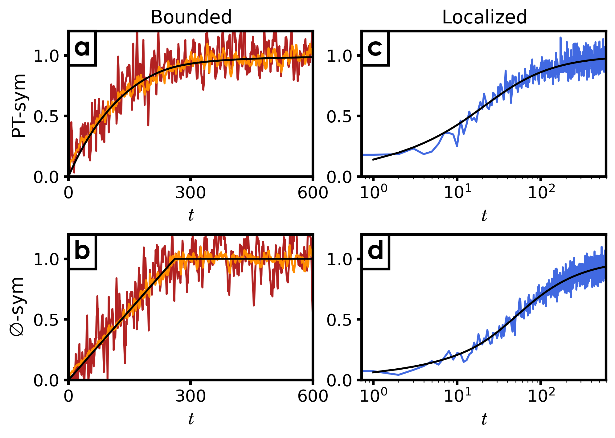
Figure A6: Analytical and Numerical Form Factor and CFS contrast, in the $\mathsf{PT}$-sym and $\varnothing$-sym shaken rotor, in the localized and classically bounded regimes. $\mathbf{(a-b)}$: In the classically bounded case: renormalized numerical CFS contrast $\mathcal{C}_{\mathrm{CFS}}(t)$ (brown curves), numerical computation of the Form Factor $\mathcal{K}(t)$ (orange curves), and analytical prediction of the Form Factor $\mathcal{K}^{O}(t)$ in $\mathbf{(a)}$ and $\mathcal{K}^{U}(t)$ in $\mathbf{(b)}$ (black curves). Parameters: $K=40$, $\hbar_{\mathrm{eff}}=1$, $N_{H}=17$, $L_{p}\approx 220$. We fit $\mathcal{K}(t)$ with the appropriate prediction to extract the Heisenberg time $t_{H}$ of the system: $\mathbf{(a)}$ $t_{H}\approx 257.7\simeq L_{p}$, corresponding to the extension of the chaotic sea. $\mathbf{(b)}$ $t_{H}\approx 261\simeq L_{p}$. $\mathbf{(c}$-$\mathbf{d)}$ Localized case: renormalized numerical CFS contrast $\mathcal{C}_{\mathrm{CFS}}(t)$ (blue curves) and analytical predictions $\mathcal{K}_{\text{loc}}^{O}(t)$ $\mathbf{(c)}$-$\mathcal{K}_{\text{loc}}^{U}(t)$ in $\mathbf{(d)}$ (black curves). Parameters: $K=20$, $\hbar_{\mathrm{eff}}=2.5$, $N_{H}=128$, $L_{p}\approx 645$. We fit the renormalized numerical CFS contrasts with the analytical predictions to extract the time $t_{H}$. $\mathbf{(c)}$ Localized $\mathsf{PT}$-symmetric shaken rotor with $t_{H}\approx 16.18$, corresponding to $\xi_{p}/\hbar_{\mathrm{eff}}$. $\mathbf{(d)}$ Localized $\varnothing$-symmetric shaken rotor with $t_{H}\approx 40.05\simeq\xi_{p}/\hbar_{\mathrm{eff}}$.

.0.3 CFS peak growth

Finally, we describe the growth of the CFS peak in the shaken rotor, comparing it in particular to its well-known dynamics in the kicked rotor. As stated in the manuscript, a key interest of the shaken rotor model is that it allows the investigation of the CFS peak in both the classically bounded ($L_{p}\ll\xi_{p}$) and dynamically localized ($L_{p}\gg\xi_{p}$) regimes, as well as in different symmetry classes—here, the Orthogonal and Unitary classes.

An important property of the CFS peak is that its growth is governed by the spectral form factor $\mathcal{K}(t)$, see e.g. [32, 57]. The form factor $\mathcal{K}(t)$ is the Fourier transform of the two-point energy correlator, defined as

$$\mathcal{K}(t)=\frac{1}{N_{S}}\left\langle\sum_{n,m}e^{-i(\epsilon_{n}-\epsilon_{m})t}\right\rangle=\frac{1}{N_{S}}\langle\lvert\text{tr}(\hat{U}^{t})\rvert^{2}\rangle,$$ (A10)

where $\hat{U}$ is the evolution operator, a unitary matrix of size $N_{S}\times N_{S}$ with $N_{S}$ the numerical model system size, and $\epsilon_{n}$ denotes its quasi-energies.

The spectral form factor $\mathcal{K}(t)$ is known analytically for certain Random Matrix Ensembles [58]. In the Gaussian Orthogonal Ensemble (GOE), it takes the form

$$\mathcal{K}^{O}(t)=\begin{cases}\frac{2t}{t_{H}}-\frac{t}{t_{H}}\log\left(1+\frac{2t}{t_{H}}\right),&\text{if }t<t_{H};\\ \\ 2-\frac{t}{t_{H}}\log\left(\frac{2t/t_{H}+1}{2t/t_{H}-1}\right),&\text{if }t\geq t_{H},\end{cases}$$ (A11)

while in the Gaussian Unitary Ensemble (GUE), it is given by

$$\mathcal{K}^{U}(t)=\begin{cases}\frac{t}{t_{H}},&\text{if }t<t_{H};\\ \\ 1,&\text{if }t\geq t_{H},\end{cases}$$ (A12)

where $t_{H}$ is the Heisenberg time.

Conversely, for 1D Anderson localization, the form factor follows [57]

$$\mathcal{K}^{O}_{\text{loc}}(t)=\left(I_{0}\left(\frac{2t_{H}}{t}\right)+I_{1}\left(\frac{2t_{H}}{t}\right)\right)\exp\left(-\frac{2t_{H}}{t}\right),$$ (A13)

in the Orthogonal class, and

$$\mathcal{K}^{U}_{\text{loc}}(t)=I_{0}\left(\frac{t_{H}}{t}\right)\exp\left(-\frac{t_{H}}{t}\right),$$ (A14)

in the Unitary class, with $I_{0,1}$ the modified Bessel functions.

The behavior of the CFS peak in the 1D Anderson localized regime was shown to correspond to $\mathcal{K}^{O,U}_{\text{loc}}(t)$ in the kicked rotor [30]. In Fig. A6, we show that this is also the case for the shaken rotor models in both the Orthogonal and Unitary symmetry classes, in the dynamically localized regime. Additionally, we consider the classically bounded case and demonstrate that it corresponds to $\mathcal{K}^{O,U}(t)$ from random matrix theory. More precisely, we examine the time evolution of the CFS contrast. Starting from an initial state peaked at $x_{0}$, the normalized contrast $\mathcal{C}_{CFS}(t)$ is defined as

$$\mathcal{C}_{CFS}(t)=(n(x_{0},t)-1)/(\lim_{t\to\infty}n(x_{0},t)-1),$$ (A15)

where $n(x_{0},t)$ is the averaged spatial probability density, given by

$$n(x_{0},t)=N_{S}\overline{\lvert\psi(x_{0},t)\rvert^{2}},$$ (A16)

The normalization coefficient $\lim_{t\to\infty}n(x_{0},t)-1$ is used in order to compare the CFS contrast with the form factor, which always reaches 1 at long times.

We have computed the CFS contrast and the form factor in the two shaken rotor models and in both the classically bounded and localized regimes (see Fig. A6). In the classically bounded case, the growth of the CFS peak follows the form factor $\mathcal{K}^{O,U}(t)$, and fitting the analytical prediction $\mathcal{K}(t)$ yields a Heisenberg time $t_{H}$ close to the chaotic sea size $L_{p}$, as expected.

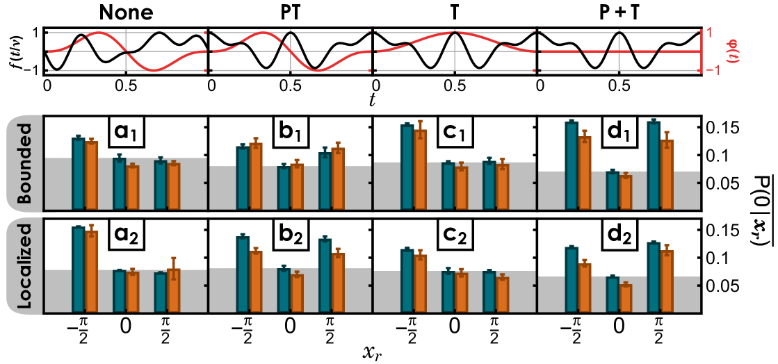
Figure A7: (top): Shape of periodic modulations of lattice depth (black) and position (red) corresponding to symmetries (none, $\mathsf{PT}$, $\mathsf{T}$, $\mathsf{P+T}$ for panels (a-d) respectively). (bottom) Experimental (orange) and numerical (blue) average probabilities $\overline{P(0,x_{r})}$ obtained for different symmetries of the modulation, and in two different localization regimes: bounded $\xi_{\rm loc}/L\gtrsim 1$, and localized $\xi_{\rm loc}/L\lesssim 0.1$, where $\xi_{\rm loc}=\xi_{p}/\hbar_{\mathrm{eff}}$ is the localization length and $L=L_{p}/\hbar_{\mathrm{eff}}$ the extension of the chaotic sea, in units of $\hbar_{\mathrm{eff}}$. The signals are obtained using the method presented in Figure 2 of the main text with an additional average over 3 modulations periods. The data shown correspond to Figure 3 of the main text.

In the localized case, we compute the CFS contrast on a logarithmic time scale. For the same system parameters, in the $\mathsf{PT}$-symmetric case, the characteristic time $t_{H}$ is approximately half of that in the $\varnothing$-symmetric case, as expected. Moreover, these characteristic times match well with the localization lengths previously computed in Fig. A5.

Average probabilities

On Figure A7, we show the average probability values at $\ell=0$, and for $x_{r}=0,\pm\pi/2$, that were obtained experimentally (orange bars) and from the full numerical modeling (blue bars). It is from these distributions that we compute the CBS and CFS contrasts, and the regimes and parameters are the ones of Figure 3 of the main article.

CBS dynamics

The CBS peak appears on short timescales, corresponding to the elastic scattering time $t_{scatt}\sim 1$, in contrast to the CFS peak, which arises around the Heisenberg time, $t_{H}$, determined by localization [30]. We can compare their dynamics in $\mathsf{PT}$-symmetry (see Fig. A8), where both peaks are expected. The figure illustrates, for a localized regime, an experimentally reconstructed Husimi distribution at short time $N=4$, showing a single peak at $x=\pi/2$ corresponding to the CBS. At longer times ($N=[15,16,17]$), using the phase space rotation method, both CBS and CFS are observed.

Figure A8: CBS dynamics in $\mathsf{PT}$ symmetry. $\mathbf{(a_{1})}$ Evolution of the averaged spatial density. $\mathbf{(a_{2})}$ Experimentally reconstructed average Husimi distribution at a short time $N=4$ (with contour plot projections lines at $50,75,90$ and $99\%$ of maximum) showing the presence of CBS.$\mathbf{(a_{3})}$ Phase space rotation signals obtained at a longer time ($N=[15,16,17]$), where both CBS and CFS are present. Parameters: $\mathsf{PT}$ symmetry, $L=20$, $\xi_{\mathrm{loc}}=2.45\pm 1.21$ .

References

- Ott [2002] E. Ott, Chaos in Dynamical Systems (Cambridge University Press, 2002).
- Gallavotti [1999] G. Gallavotti, Statistical Mechanics (Springer, Berlin, Heidelberg, 1999).
- D’Alessio et al. [2016] L. D’Alessio, Y. Kafri, A. Polkovnikov, and M. Rigol, Advances in Physics 65, 239 (2016).
- Gogolin and Eisert [2016] C. Gogolin and J. Eisert, Rep. Prog. Phys. 79, 056001 (2016).
- Ueda [2020] M. Ueda, Nature Reviews Physics 2, 669 (2020).
- Anderson [1958] P. W. Anderson, Phys. Rev. 109, 1492 (1958).
- Evers and Mirlin [2008] F. Evers and A. D. Mirlin, Rev. Mod. Phys. 80, 1355 (2008).
- Abrahams [2010] E. Abrahams, ed., 50 Years of Anderson Localization (World Scientific, 2010).
- Santhanam et al. [2022] M. Santhanam, S. Paul, and J. B. Kannan, Physics Reports 956, 1 (2022).
- Abanin et al. [2019] D. A. Abanin, E. Altman, I. Bloch, and M. Serbyn, Rev. Mod. Phys. 91, 021001 (2019).
- Alet and Laflorencie [2018] F. Alet and N. Laflorencie, Comptes Rendus Physique 19, 498 (2018).
- Tikhonov and Mirlin [2021] K. S. Tikhonov and A. D. Mirlin, Annals of Physics 435, 168525 (2021).
- Sierant et al. [2025] P. Sierant, M. Lewenstein, A. Scardicchio, L. Vidmar, and J. Zakrzewski, Rep. Prog. Phys. 88, 026502 (2025).
- Serbyn et al. [2021] M. Serbyn, D. A. Abanin, and Z. Papić, Nature Physics 17, 675 (2021).
- Zhao et al. [2024] L. Zhao, P. R. Datla, W. Tian, M. M. Aliyu, and H. Loh, (2024), arXiv:2403.09517 [quant-ph] .
- Adler et al. [2024] D. Adler, D. Wei, M. Will, K. Srakaew, S. Agrawal, P. Weckesser, R. Moessner, F. Pollmann, I. Bloch, and J. Zeiher, Nature 636, 80 (2024).
- Tindall et al. [2020] J. Tindall, C. Sánchez Muñoz, B. Buča, and D. Jaksch, New J. Phys. 22, 013026 (2020).
- Ho et al. [2023] W. W. Ho, T. Mori, D. A. Abanin, and E. G. Dalla Torre, Annals of Physics 454, 169297 (2023).
- Bohigas et al. [1993] O. Bohigas, S. Tomsovic, and D. Ullmo, Physics Reports 223, 43 (1993).
- Akkermans and Montambaux [2007] E. Akkermans and G. Montambaux, Mesoscopic physics of electrons and photons (Cambridge University Press, 2007).
- Hainaut et al. [2018] C. Hainaut, I. Manai, J.-F. Clément, J. C. Garreau, P. Szriftgiser, G. Lemarié, N. Cherroret, D. Delande, and R. Chicireanu, Nat. Commun. 9, 1382 (2018).
- Jendrzejewski et al. [2012] F. Jendrzejewski, K. Müller, J. Richard, A. Date, T. Plisson, P. Bouyer, A. Aspect, and V. Josse, Phys. Rev. Lett. 109, 195302 (2012).
- Haake [1991] F. Haake, Quantum signatures of chaos (Springer, 1991).
- Bohigas et al. [1984] O. Bohigas, M. J. Giannoni, and C. Schmit, Phys. Rev. Lett. 52, 1 (1984).
- Hasan and Kane [2010] M. Z. Hasan and C. L. Kane, Rev. Mod. Phys. 82, 3045 (2010).
- Parameswaran and Vasseur [2018] S. Parameswaran and R. Vasseur, Rep. Prog. Phys. 81, 082501 (2018).
- Karpiuk et al. [2012] T. Karpiuk, N. Cherroret, K. L. Lee, B. Grémaud, C. A. Müller, and C. Miniatura, Phys. Rev. Lett. 109, 190601 (2012).
- Ghosh et al. [2014] S. Ghosh, N. Cherroret, B. Grémaud, C. Miniatura, and D. Delande, Phys. Rev. A 90, 063602 (2014).
- Lee et al. [2014] K. L. Lee, B. Grémaud, and C. Miniatura, Phys. Rev. A 90, 043605 (2014).
- Lemarié et al. [2017] G. Lemarié, C. A. Müller, D. Guéry-Odelin, and C. Miniatura, Phys. Rev. A 95, 043626 (2017).
- Ghosh et al. [2017] S. Ghosh, C. Miniatura, N. Cherroret, and D. Delande, Phys. Rev. A 95, 041602 (2017).
- Martinez et al. [2023] M. Martinez, G. Lemarié, B. Georgeot, C. Miniatura, and O. Giraud, SciPost Physics 14, 10.21468/scipostphys.14.3.057 (2023).
- Arabahmadi et al. [2024] E. Arabahmadi, D. Schumayer, B. Grémaud, C. Miniatura, and D. A. W. Hutchinson, Phys. Rev. Res. 6, L012021 (2024).
- Billy et al. [2008] J. Billy, V. Josse, Z. Zuo, A. Bernard, B. Hambrecht, P. Lugan, D. Clément, L. Sanchez-Palencia, P. Bouyer, and A. Aspect, Nature 453, 891–894 (2008).
- Chabé et al. [2008] J. Chabé, G. Lemarié, B. Grémaud, D. Delande, P. Szriftgiser, and J. C. Garreau, Phys. Rev. Lett. 101, 255702 (2008).
- Madani et al. [2024] F. Madani, M. Denis, P. Szriftgiser, J.-C. Garreau, A. Rançon, and R. Chicireanu, (2024), arXiv:2402.06573 .
- Hainaut et al. [2017] C. Hainaut, I. Manai, R. Chicireanu, J.-F. Clément, S. Zemmouri, J.-C. Garreau, P. Szriftgiser, G. Lemarié, N. Cherroret, and D. Delande, Phys. Rev. Lett. 118, 184101 (2017).
- Sajjad et al. [2022] R. Sajjad, J. L. Tanlimco, H. Mas, A. Cao, E. Nolasco-Martinez, E. Q. Simmons, F. L. N. Santos, P. Vignolo, T. Macrì, and D. M. Weld, Phys. Rev. X 12, 011035 (2022).
- Moore et al. [1994] F. L. Moore, J. C. Robinson, C. Bharucha, P. E. Williams, and M. G. Raizen, Phys. Rev. Lett. 73, 2974 (1994).
- Casati et al. [1979] G. Casati, B. V. Chirikov, I. F. M., and J. Ford, in Stochastic Behavior in Classical and Quantum Hamiltonian Systems, Lecture Notes in Physics, Vol. 93, edited by G. Casati and J. Ford (Springer, Berlin, 1979).
- Wolf and Maret [1985] P.-E. Wolf and G. Maret, Phys. Rev. Lett. 55, 2696 (1985).
- Sakai et al. [1997] K. Sakai, K. Yamamoto, and K. Takagi, Phys. Rev. B 56, 10930 (1997).
- Wiersma et al. [1997] D. S. Wiersma, P. Bartolini, A. Lagendijk, and R. Righini, Nature 390, 671 (1997).
- Labeyrie et al. [1999] G. Labeyrie, F. de Tomasi, J.-C. Bernard, C. A. Müller, C. Miniatura, and R. Kaiser, Phys. Rev. Lett. 83, 5266 (1999).
- Huang et al. [2001] J. Huang, N. Eradat, M. E. Raikh, Z. V. Vardeny, A. A. Zakhidov, and R. H. Baughman, Phys. Rev. Lett. 86, 4815 (2001).
- Bromberg et al. [2016] Y. Bromberg, B. Redding, S. M. Popoff, and H. Cao, Phys. Rev. A 93, 023826 (2016).
- Altland and Zirnbauer [1996] A. Altland and M. R. Zirnbauer, Phys. Rev. Lett. 77, 4536 (1996).
- Dupont et al. [2021] N. Dupont, G. Chatelain, L. Gabardos, M. Arnal, J. Billy, B. Peaudecerf, D. Sugny, and D. Guéry-Odelin, PRX Quantum 2, 040303 (2021).
- Dupont et al. [2023] N. Dupont, F. Arrouas, L. Gabardos, N. Ombredane, J. Billy, B. Peaudecerf, D. Sugny, and D. Guéry-Odelin, New Journal of Physics 25, 013012 (2023).
- Chirikov [1979] B. V. Chirikov, Phys. Rep. 52, 263 (1979).
- Delande [2013] D. Delande, Kicked rotor and Anderson localization, Boulder School on Condensed Matter Physics (2013), lecture I.
- Mouchet et al. [2001] A. Mouchet, C. Miniatura, R. Kaiser, B. Grémaud, and D. Delande, Phys. Rev. E 64, 016221 (2001).
- Rechester and White [1980] A. B. Rechester and R. B. White, Phys. Rev. Lett. 44, 1586 (1980).
- Pichard et al. [1990] J.-L. Pichard, M. Sanquer, K. Slevin, and P. Debray, Phys. Rev. Lett. 65, 1812 (1990).
- Blümel and Smilansky [1992] R. Blümel and U. Smilansky, Phys. Rev. Lett. 69, 217 (1992).
- Shepelyansky [1987] D. Shepelyansky, Physica D: Nonlinear Phenomena 28, 103 (1987).
- Marinho and Micklitz [2018] M. Marinho and T. Micklitz, Phys. Rev. B 97, 041406(R) (2018).
- M.J. Giannoni and Zinn-Justin [1991] A. V. M.J. Giannoni and J. Zinn-Justin, Les Houches 1989 Session LII, Chaos and Quantum Physics (North-Holland, 1991) pp. 189–191.