Structure-Preserving Neural Ordinary Differential Equations for Stiff Systems

Abstract

Neural ordinary differential equations (NODEs) are an effective approach for data-based modeling of dynamical systems arising from simulations and experiments. One of the major shortcomings of NODEs, especially when coupled with explicit integrators, is its long-term stability, which impedes their efficiency and robustness when encountering stiff problems. In this work we present a structure-preserving NODE approach, which integrates with a linear and nonlinear split and an exponential integrator, latter of which is an explicit integrator with stability properties comparable to implicit methods. We demonstrate that our model has advantages in both learning and deployment over standard explicit or even implicit NODE methods. The long-time stability is further enhanced by the Hurwitz matrix decomposition that constrains the spectrum of the linear operator, therefore stabilizing the linearized dynamics. When combined with a Lipschitz-controlled neural network treatment for the nonlinear operator, we show the nonlinear dynamics of the NODE are provably stable in the sense of Lyapunov. For high-dimensional data, we further rely on an autoencoder performing dimension reduction and Higham’s algorithm for the matrix-free application of the matrix exponential on a vector. We demonstrate the effectiveness of the proposed NODE approach in various examples, including the Grad-13 moment equations and the Kuramoto-Sivashinky equation.

1 Introduction

Data-driven reduced order models (ROMs) of dynamical systems arising from high-resolution simulations or experiments can be used as efficient forward-model surrogates. The learned surrogates can be deployed in the traditionally expensive tasks of optimization and parameter inference. However, conventional data-driven ROMs for dynamical systems generally struggle with accurately approximating stiff dynamical systems [14] and maintaining long-term stability [17, 21]. In this work, we address both of these challenges in the context of neural ordinary differential equations (NODEs) [3], which are a class of models that approximate dynamical systems continously as ODEs using neural networks. The two ingredients that determine the effectiveness of NODE-based models are the neural network architecture and the numerical integrator. For the former we proposed a structure-preserving NODE, which integrates with a linear and nonlinear split and several small components that preserve key mathematical structures strongly. For the latter we incorporate NODE with advanced time stepping through exponential integrators. The use of an exponential integrator improves upon the performance of explicit and semi-implicit integrators that are commonly used in packages such as diffrax [13] and torchode [16].

In [17], motivated by the inertial manifold theorem, we developed a special NODE approach that embeds a linear and nonlinear partition of the right-hand-side (RHS) being approximated by two neural networks. This partitioning method provides better short-time tracking, prediction of the energy spectrum, and robustness to noisy initial conditions than standard NODEs. The recent work [23, 24] extended the linear and nonlinear partition to a semi-implicit NODE. In the forward pass of their training they solve a partitioned ODE using implicit-explicit Runge-Kutta (IMEX-RK) methods.

The linear and nonlinear partition allows them to avoid solving a fully nonlinear system. The backward pass is handled through a discrete adjoint approach, resulting into a linear system to be solved. In general, the matrices from these linear systems will be dense, requiring a direct solve which can be computationally expensive and have poor scalability. Our NODE uses an explicit approach based on exponential integrators, which do not require direct solvers but enjoy the stability property comparable to an implicit approach. The recent work [7] performs a preliminary study for applying exponential integration schemes in NODEs. It shows exponential integration is able to handle a low-dimensional ODE where implicit schemes failed. However, this work shows the straightforward implementation of exponential integrators to be too computationally expensive for practical purposes. Our work relies on several key components to overcome the challenge of training when applying such an exponential integrator with NODE to high-dimensional problems.

The contributions of our work are two-fold: the structures strongly built into NODEs and improvement in time stepping and training. For structures, the linear and nonlinear partitioning is built explicitly into our NODE and parameterized separately. The linear part of the system is parameterized using a novel Hurwitz matrix decomposition [5], which aids in long-term stability by constraining the spectrum (all eigenvalues have negative real part). For the nonlinear part we apply either a bilinear form or a Lipshitz controlled neural network proposed in our previous work [21]. The bilinear form has the advantage of clearly separating the linear and nonlinear dynamics which helps accurately capture the spectrum. A multilayer perceptron (MLP) approximation to the nonlinear part like those used in [17] will not exclude the linear contribution. In contrast, imposing the bilinear form excludes the linear dynamics contribution, which forces the linear and nonlinear separation. The Lipshitz controlled neural network on the other hand can provide stable long-term predictions. Our other major contribution involves using an exponential integrator for the time integration with a matrix-free implementation developed in [1]. For cases with high-dimensional data we use an autoencoder to aid in our training. Evolving our dynamics on a low-dimensional latent space while preserving the linear and nonlinear partition allows a significant reduction in training time while retaining the stability of the model. Note that latent dynamics discovery has seen success in other scientific machine learning approaches [6, 22].

The rest of the paper is organized as follows. Section 2 presents the details behind the parameterizations of the linear and nonlinear parts of NODE along with implementation details. Section 3 gives a result about the Liapunov stability and provides an error bound for the NODE. Section 4 provides a brief introduction to exponential integrators. The details related to training and their results are given in Section 5. Conducing remarks are given in 6.

2 Structure-Preserving NODE

This work focuses on dynamical systems that can be transformed into systems of the form

(1) $$\frac{du}{dt}=Au+g(u),$$

where $u\in\mathbb{R}^{n}$, $g:\mathbb{R}^{n}\rightarrow\mathbb{R}^{n}$ is a nonlinear function, and $A\in\mathbb{R}^{n\times n}$ has eigenvalues whose real parts are bounded above by a known estimate $\mu$. Many semi-discretized time-dependent PDEs, such as the Navier-Stokes equations and Kuramoto-Sivashinsky equation, can be modeled using this framework.

Our proposed structure-preserving NODE takes the form

(2) $$\frac{du}{dt}=A_{L}u+g_{NN}(u).$$

Here the linear trainable matrix $A_{L}$ is parameterized using $A_{L}=A_{H}+I\mu$, where $A_{H}$ has eigenvalues that all have negative real part. The estimate for $\mu$ is problem specific. For example, if the linearized dynamics are known to be dissipative, then $\mu=0$ is a suitable choice. In the case of Kuramoto-Sivashinky considered in Section 5.3, we applied a Fourier analysis to the equations to determine an estimate. Section 2.1 describes how $A_{H}$ can be parameterized using a Hurwitz matrix decomposition. The nonlinear operator, $g_{NN}$, is parameterized using either a bilinear form neural network or a Lipschitz controlled neural network, as described in Sections 2.2 and 2.3, respectively.

2.1 Hurwitz Matrix Parameterization

A matrix where all the eigenvalues have negative real parts is a Hurwitz matrix. We develop a general decomposition for a Hurwitz matrix based on the following theorem.

A matrix $A_{H}\in\mathbb{R}^{n\times n}$ is Hurwitz stable if and only if there exists a symmetric negative-definite matrix $G_{s}$, skew symmetric matrix $G_{u}$, and a symmetric positive-definite matrix $S$ such that

(3) $$A_{H}=(G_{s}+G_{u})S.$$

This theorem and its proof can be found in [5].

The Cholesky factorization, which involves a product of a lower triangular matrix with its transpose, is a parameterization for symmetric positive definite matrices and involves $\frac{n(n+1)}{2}$ unique parameters. The Cholesky factorization is used to parameterize $S$ and $G_{s}$,

(4a) $$S =L^{S}(L^{S})^{T},$$

(4b) $$G_{s} =-L^{G}(L^{G})^{T},$$

where $L^{S}$ and $L^{G}$ are lower triangular matrices. The skew-symmetric matrix $G_{u}$ is formed using

(5) $$G_{u}=L_{s}-L_{s}^{T},$$

where $L_{s}$ is a strictly lower triangular matrix, $L_{s}$ and therefore requires $\frac{n(n-1)}{2}$ unique parameters. The matrix $A_{H}$ is thus parameterized by a combination of $L^{S}$, $L^{G}$, and $L_{s}$. The total number of parameters needed to describe $A_{H}$ is $\frac{3n^{2}+n}{2}$.

2.2 Bilinear Form Neural Network

One option to approximate the nonlinear part, $g$, is to use a bilinear form. By construction, the bilinear form will have zero contribution to the linear operator since it is built with quadratic forms. This property is not guaranteed when using a vanilla feed-forward network for $g$. This creates a strict separation of the linear and nonlinear dynamics that allows recovery of the linear operator $A$ in an equation learning setting. We utilize the low rank-bilinear form network as defined in [21]. It is defined by

(6) $$g_{NN}(u)=\sum\limits_{r=1}^{R}(C^{(r)}u)\odot(D^{(r)}u)+b,$$

where $u\in\mathbb{R}^{n},\ C^{(r)}\in\mathbb{R}^{n\times n},\ D^{(r)}\in\mathbb{R}^{n\times n},$ $b\in\mathbb{R}^{n\times 1}$, $\odot$ represents the Hadamard product (element-wise multiplication), and $R,\ 1\leq R\leq n$ represents the rank of approximation which will be chosen much smaller than $n$ during the training.

2.3 Lipschitz Controlled Neural Network

The second option we explore to approximate $g$ with is a neural network with a bounded Lipschitz constant. As shown in Section 3.1, having a Lipschitz bound on $g_{NN}$ has an impact on the long-term stability of the dynamics. We introduce a novel Lipschitz-controlled neural network architecture. The network is a feedforward network given by

(7) $$g_{NN}(u)=l_{p}\odot l_{p-1}\dots\odot l_{1}(u)$$

where

(8) $$l_{i}(z)=\sigma(B_{i}z+b_{i}),\qquad B_{i}=L^{1/p}\frac{W_{i}}{\max(1,\,\sqrt{\|W_{i}\|_{\infty}\|W_{i}\|_{1}})},$$

$W_{i}\in\mathbb{R}^{n_{i}\times n_{i+1}}$ are trainable matrices, $n_{1}=n_{p+1}=n$, $n_{2}=\dots=n_{p}=d$ is a chosen latent dimension and $\sigma$ is a $1$-Lipschitz activation function. $L>0$ is the desired Lipschitz constant of the network $g_{NN}$.

Note that the $1$-norm and $\infty$-norm of a matrix are the maximum absolute column sum and the maximum absolute row sum, respectively. Therefore, the realization of $B_{i}$ can be implemented in a manner compatible with automatic differentiation. The following theorem shows $g_{NN}$ has the desired property. The network $g_{NN}(u)$ given in Definition 2.3 is $L$-Lipschitz.

Proof.

First, we show each layer $l_{i}$ is $L^{1/p}$-Lipschitz. If $z_{1}$ and $z_{2}$ are inputs for $l_{i}$, then

$$\|l_{i}(z_{1})-l_{i}(z_{2})\|_{2} =\|\sigma(B_{i}z_{1}+b_{i})-\sigma(B_{i}z_{2}+b_{i})\|_{2}$$

$$\leq\|\sigma\|_{2}\|B_{i}z_{1}+b_{i}-(B_{i}z_{2}+b_{i})\|_{2}$$

$$\leq\|B_{i}(z_{1}-z_{2})\|_{2}$$

$$\leq\|B_{i}\|_{2}\|z_{1}-z_{2}\|_{2}.$$

The operator norm of $B_{i}$ may be bounded as follows

$$\|B_{i}\|_{2} =L^{1/p}\frac{\|W_{i}\|_{2}}{\max\left(1,\sqrt{\|W_{i}\|_{1}\|W_{i}\|_{\infty}}\right)}\leq L^{1/p},$$

in which the inequality follows a special case of Hölder’s inequality, $\|W_{i}\|_{2}\leq\sqrt{\|W_{i}\|_{1}\|W_{i}\|_{\infty}}$. Therefore, each layer is $L^{1/p}$-Lipschitz. It follows that the network $g_{NN}$ is $L$-Lipshitz.

Our previous work [21] introduced a bi-Lipschitz affine transformation (bLAT) network, achieving Lipschitz control using a parameterization based on the singular value decomposition (SVD). The parameteization presented here is more efficient since the SVD is more expensive to evaluate than the $1$ and $\infty$ norms. However, unlike the above, the bLAT network is bi-Lipschitz.

2.4 Autoencoder

Inspired by the seminal work [19] for complex dynamical systems involving high-dimensional data, an autoencoder produces an low dimensional representation of the dynamics which can be integrated efficiently. For high-dimensional problems like the Kuramoto-Sivashinsky equation, we find it is necessary to include the dimension reduction in structure-preserving NODE to avoid training directly on a high-dimensional space, which is more challenging and expensive.

We consider some dynamical system for $U(t)\in\mathbb{R}^{m}$ and assume that it can be transformed into a variable $u\in\mathbb{R}^{n}$, $n<m$ where the dynamics are described by a system of the form (1). Two feed-forward neural networks are trained $f_{E}(U;\alpha)$ and $f_{D}(u;\beta)$, which represent the encoder and decoder and have network parameters $\alpha$ and $\beta$, respectively. The network $f_{E}:\mathbb{R}^{m}\to\mathbb{R}^{n}$ takes in the initial condition in physical space and network parameters and outputs the initial condition in the lower-dimensional latent space $\mathbb{R}^{n}$. Once the initial condition is projected onto the latent space we use a time integrator to evolve the dynamics forward in time. By evolving the dynamics in the low-dimensional latent space $\mathbb{R}^{n}$, efficiency is gained in the numerical integration step. In mathematical symbols we have $f_{E}(U_{0})=u_{0}$ then we evolve $u_{0}$ several timesteps (using the exponential integrator in this work) to obtain $\{u_{1},u_{2},\dots,u_{k}\}$. After this, these are each transformed back into the full space data using the decoder $U_{i}=f_{D}(u_{i})$, which are then used to compute the loss term. A schematic of this process is given in Figure 1.

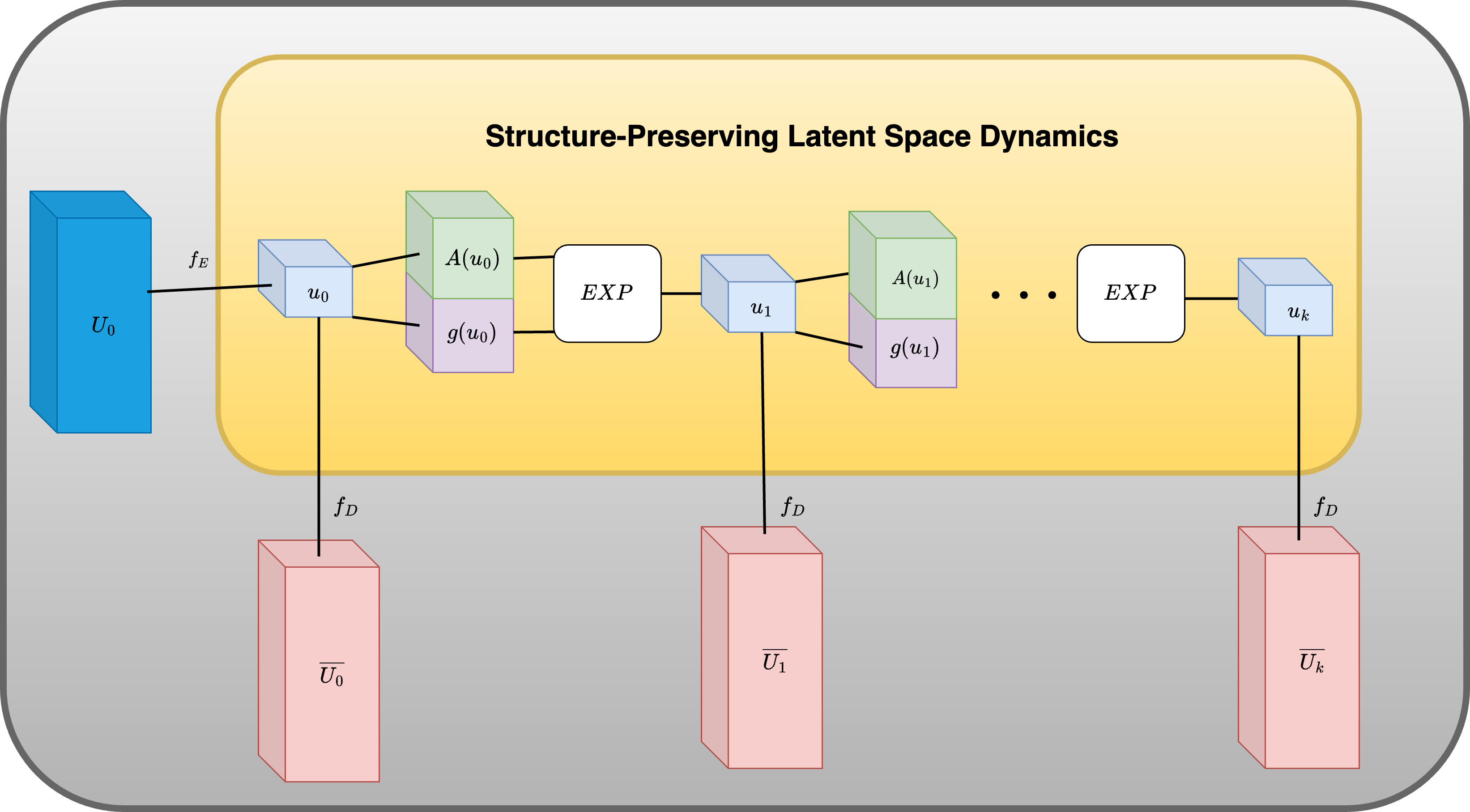
Figure 1: Schematic of the autoencoder for our structure preserving NODE. The dark blue block represents the initial data which is encoded using $f_{E}$ into the light blue block representing the initial condition in the latent space. The green and purple blocks represent the neural networks for the linear and nonlinear operators, respectively. These neural networks are used to push the dynamics forward using the exponential integrator defined in (15). The data in the latent space is then decoded back into physical space using $f_{D}$. Decoded data is represented by the pink blocks.

3 Analysis of the Network

This section gives two results about the proposed structure-preserving NODE. In Section 3.1 Liapunov stability of the network is demonstrated, and in Section 3.2 an error bound for the network is given.

3.1 Liapunov Stability of the Network

The NODE is parameterized such that the spectrum of the linear operator $A_{L}$ is bounded from above by some $\mu\in\mathbb{R}$. In the case of $\mu<0$, we will show that any fixed point is an asymptotically stable attractor for the dynamical system defined by the NODE when a constraint on the nonlinear part is satisfied.

If the structure-preserving NODE (2) is parameterized such that the linear operator $A_{L}$ satisfies ${\rm Re}(\lambda(A_{L}))\leq\mu<0$ and for $\epsilon>0$ there exists a $\delta>0$ such that $\|g_{NN}(u)-g_{NN}(u^{*})\|\leq\epsilon\|u-u^{*}\|$ for $\|u-u^{*}\|\leq\delta$ implies the NODE is stable in the sense of Liapunov at any fixed point $u^{*}$.

Proof.

Without loss of generality, assume $u^{*}=0$. It suffices to show the existence of a Liapunov function, $V(u)$, such that $V(u)\geq 0,V(u)=0$ if and only if $u=0$, and $\frac{d}{dt}V(u)\leq 0$ for all $t>0$. Let $T$ be a matrix where the columns of the matrix are the eigenvectors of $A_{L}$. We introduce the change of variables $z(u)=T^{-1}u$. If we define $V(u)=\|z(u)\|^{2}$, then

$$\frac{d}{dt}V(u) =\frac{d}{dt}\|z\|^{2}$$

$$=2\left\langle z,\frac{d}{dt}z\right\rangle$$

$$=2\langle z,T^{-1}A_{L}Tz\rangle+2\langle z,T^{-1}g_{NN}(Tz)\rangle$$

$$\leq 2\mu\|z\|^{2}+2\|z\|\|T^{-1}\|\|g_{NN}(Tz)\|$$

When $\|u\|\leq\delta$, we have

$$\leq 2\mu\|z\|^{2}+2\|z\|\|T^{-1}\|\epsilon\|T\|\|z\|$$

$$=2(\mu+\epsilon\|T^{-1}\|\cdot\|T\|)V(u).$$

When $\epsilon<\frac{|\mu|}{\|T^{-1}\|\cdot\|T\|}$, the right hand side is negative. This shows $V(u)$ is a Liapunov function which implies Liapunov stability.

3.2 Bounding the Error of a Learned Model

Given an estimate on the approximation error of the learned operators, a bound can be obtained for the error between the ground truth and learned dynamics.

Suppose that $u(t)$ is a solution of the system of differential equations $u^{\prime}=Au+g(u)$, $u(t_{0})=u_{0}$, $v(t)$ is and approximate solution generated by structure-preserving NODE where $\|v\|\leq\mathcal{V}$. If $u$ and $v$ are differentiable, then the error between the two trajectories is bounded by

(9) $$\|u(t)-v(t)\|\leq\rho e^{(||A||+L)(t-t_{0})}+\frac{(\|dA\|+\|dg\|)\mathcal{V}}{||A||+L}\left(e^{(||A||+L)(t-t_{0})}-1\right).$$

Here $\rho$ is the error in the initial condition. $dA$ and $dg$ is the difference between the neural network operators and the ground truth for $A$ and $g$, respectively, and $L$ is the Lipschitz constant for $g_{NN}$.

Proof.

If $m(t)=\|v(t)-y(t)\|$, then

$$\frac{dm(t)}{dt} =\lim\limits_{h\to 0}\frac{m(t+h)-m(t)}{h}$$

$$=\lim\limits_{h\to 0}\frac{\|v(t+h)-u(t+h)\|-\|v(t)-u(t)\|}{h}$$

$$\leq\lim\limits_{h\to 0}\frac{\|v(t+h)-u(t+h)-(v(t)-u(t))\|}{h}$$

$$=\|v^{\prime}(t)-u^{\prime}(t)\|$$

$$=\|A_{L}v+g_{NN}v-(Au+gu)\|$$

$$=\|A_{L}v+g_{NN}v-(Av+gv)+(Av+gv)-(Au+gu)\|$$

$$\leq(\|dA\|+\|dg\|)\|v\|+(\|A\|+L)\|v-u\|$$

$$\leq(\|dA\|+\|dg\|)\mathcal{V}+(\|A\|+L)m(t)$$

Integrating we obtain the result in (9).

4 Exponential Integrators

The proposed NODE form $\eqref{eq:linearPlusNonlinear}$ assumes a linear and nonlinear split where the stiffness of the system shall come primarily from the linear matrix $A$. For such a system, the exponential integrator is an ideal technique to overcome its stiffness, which will be leveraged in this work in the NODE training. In this section a brief review exponential integrators is presented. For an in depth introduction see [11]. Consider a system that may be written in the form

(10) $$\frac{du}{dt}=Au+g(u),\quad u(t_{0})=u_{0},\quad t\geq t_{0},$$

where $u\in\mathbb{R}^{n},\ A\in\mathbb{R}^{n\times n}$, and $g:\mathbb{R}^{n}\rightarrow\mathbb{R}^{n}$ is a nonlinear function. The solution of (10) satisfies the nonlinear integral equation

(11) $$u(t)=e^{(t-t_{0})A}u_{0}+\int\limits_{t_{0}}^{t}e^{(t-\tau)A}g(\tau,u(\tau))\ d\tau.$$

A $p$-th order Taylor series expansion of $g$ about $t_{0}$ gives

(12) $$u(t)=e^{(t-t_{0})A}u_{0}+\sum\limits_{k=1}^{p}\varphi_{k}((t-t_{0})A)(t-t_{0})^{k}g_{k}+O((t-t_{0})^{p+1}),$$

where

$$g_{k}=\left.\frac{d^{k-1}}{dt^{k-1}}g(t,u(t))\right|_{t=t_{0}},\quad\varphi_{k}(z)=\frac{1}{(k-1)!}\int\limits_{0}^{1}e^{(1-\theta)z}\theta^{k-1}\ d\theta,\quad k\geq 1.$$

The functions $\varphi_{l}(z)$ satisfy the recurrence relation

$$\varphi_{l+1}(z)=\frac{\varphi_{l}(z)-\frac{1}{l!}}{z},\quad\varphi_{0}(z)=e^{z},$$

and have the Taylor series expansion

$$\varphi_{l}(z)=\sum\limits_{k=0}^{\infty}\frac{z^{k}}{(k+l)!}.$$

Evaluating the $\varphi$ functions is a nontrivial task. The computation of $\varphi_{1}$ is a well known problem in numerical analysis [8, 10, 18]. Ref. [1] shows that it is possible to avoid computing the $\varphi$ functions (12) by solving a system with a single matrix exponential of size $(n+p)\times(n+p)$, where $n$ is the dimension of the system and $p$ is the order of the approximation. The system (1) is approximated using

(13) $$\hat{u}(t)=\begin{bmatrix}I_{n}&0\end{bmatrix}\exp\left((t-t_{0})\begin{bmatrix}A&W\\ 0&J\end{bmatrix}\right)\begin{bmatrix}u_{0}\\ e_{p}\end{bmatrix},$$

where $e_{p}$ is a vector with a $1$ in the $p^{\rm th}$ element and $0$’s elsewhere and $W\in\mathbb{R}^{n\times p}$ and $J\in\mathbb{R}^{p\times p}$ are defined to be

(14) $$J=\begin{bmatrix}0&I_{p-1}\\ 0&0\end{bmatrix},\qquad W_{ij}=\begin{cases}g_{k},&j=p-k+1\\ 0,&\text{otherwise}\end{cases}.$$

$I_{n}$ and $I_{p-1}$ are identity matrices with sizes $\mathbb{R}^{n\times n}$ and $\mathbb{R}^{p-1\times p-1}$, respectively. When $p=1$, then $W=u_{0}$ and $J=0$. Thus, for $p=1$, (13) reduces to

(15) $$\hat{u}(t)=\begin{bmatrix}I_{n}&0\end{bmatrix}\exp\left((t-t_{0})\begin{bmatrix}A&g_{0}\\ 0&0\end{bmatrix}\right)\begin{bmatrix}u_{0}\\ 1\end{bmatrix}.$$

A matrix-free algorithm developed in [1] is used to compute (15). This algorithm adapts the scaling and squaring method [9] by computing $e^{tA}b\approx(T_{m}(s^{-1}tA))^{s}b$, where $T_{m}$ is a truncated Taylor series. Algorithmically, the computation is performed using

(16) $$e^{tA}b\approx\texttt{expmv}(A,b,t)=f_{s},$$

where $f_{s}$ is defined by the following recurrence relations

(17a) $$b_{1,0} =b,$$

(17b) $$b_{i,k} =\frac{t}{sk}Ab_{i,k-1},\qquad i=1,\dots,s,\quad k=1,\dots,m$$

(17c) $$b_{i+1,0}=f_{i} =\sum_{k=0}^{m}b_{i,k},\qquad i=1,\dots,s$$

The choice of $s$ and $m$ impact both accuracy and efficiency. The number of matrix vector multiplications is $sm$ and an analysis for the optimal choice of $s$ and $m$ may be found in [1]. In practice, we choose $s$ to be proportional to the maximum time step of the training data and the norm of $A$, $s\sim\Delta t_{\rm max}\|A\|_{2}$, and we choose $m$ such that (17c) converges to some tolerance, $\tau$. Utilizing the matrix-free computation eliminates the need to compute the matrix exponential in equation (13), and can provide a faster alternative when the dimension of $A$ is large. Moreover, the computation of a matrix exponential is required for each trajectory due to the time dependency. Batching of data is improved since a matrix-free algorithm allows for vectorization. This form is used to evolve the dynamics for the structure-preserving NODE in Section 5. Note that higher-order versions of this scheme require the derivatives of the solution.

Exponential integrators are explicit methods, but enjoy stability properties comparable to implicit methods. These methods are used to solve two types of stiff problems. The first are systems with a Jacobian whose eigenvalues has large negative real parts. These systems usually arise in the discretization of parabolic partial differential equations. The second type of problems are systems that are highly oscillatory in nature these systems have purely imaginary eigenvalues. The focus of this paper is on the former.

5 Numerical Examples

In this section the structure-preserving NODE framework will be applied to three examples, including a weakly nonlinear system with transient growth, the Grad-13 moment system, and the Kuramoto-Sivashinsky equation. The first example highlights the benefits of using and exponential integrator compared to an implicit-explicit (IMEX) integration scheme, which includes improved accuracy when learning dynamics using large time steps.

Moreover, we demonstrate that the properties of the exponential integrator allow us to deploy our NODE using different time steps than those used for training. We further show that the learned model can be integrated backwards in time accurately. The Grad-13 example highlights the ability to deal with a problem which has multiple temporal scales. Finally, the Kuramoto-Sivashinsky equation demonstrates learning chaotic dynamics using our NODE.

Training details

The input to the NODE is a set of initial conditions and the output a the set of trajectories evolved from the initial conditions. For the linear part of the proposed NODE, the proposed parameterization is used for the Hurwitz matrix learning. For the nonlinear part, either a bilinear form or a feed-forward neural network with Lipschitz controlled layers is used. The networks have 2 layers with 100 to 200 hidden dimensions. The activation function is $\tanh$. The autoencoder is made up of two simple feed-forward neural networks one for the encoder and one for the decoder. The loss is computed using an approximation to the time integral of the mean squared error of the, given by

(18) $$L(t,U,\tilde{U})=\sum_{n=0}^{N_{t}-1}\frac{1}{2}\left((U_{n+1}-f_{D}(\tilde{u}_{n+1}))^{2}+(U_{n}-f_{D}(\tilde{u}_{n}))^{2}\right)(t_{n+1}-t_{n}),$$

where the initial latent variable is projected through $\tilde{u}_{0}=f_{E}(U_{0})$. Note that the loss is computed in the original coordinates; thus, the autoencoder is optimized along with the NODE during optimization step. The inclusion of this autoencoder network is optional in our framework. Our implementation of the NODE uses Jax [2] as a backend. Automatic differentiation is used to compute gradients of the loss function with respect to the trainable parameters, and the Adam optimizer from the Optax [4] package is used for optimizations.

5.1 Taming Transient Growth

In this first example we apply our structure-preserving NODE to learn the transient growth for a simple system. We focus on a weakly nonlinear dynamical system in which the right-hand-side can be decomposed into the sum of linear and nonlinear operators,

(19) $$\frac{dx}{dt}=Ax+\epsilon\sin(x),\quad x(0)=x_{0},$$

where $\sin(x)$ is interpreted to be a component-wise application of the function. The linear operator, $A$, is chosen such that in the limit of $\epsilon\to 0$ there is initial transient growth followed by long-term decay. This example is influenced by work done in [15] where the author analyzes how the norm of the matrix exponential contributes to the runtime of quantum algorithms for linear ordinary differential equations (i.e., $\epsilon=0$). Some relevant quantities used in their analysis are

(20a) $$\alpha(A) =\max\{\text{Re}(\lambda)\;|\;\lambda\in\sigma(A)\}$$

(20b) $$\gamma(A) =\max\left\{\lambda\;|\;\lambda\in\sigma\left((A+A^{T})/2\right)\right\},$$

where $\sigma(\cdot)$ represents the the set of eigenvalues of the argument. The values of $(\alpha,\gamma)$ describe the long term behavior of the norm of $e^{At}$. We focus on the case when $\alpha<0$, which implies $\lim\limits_{t\to\infty}||e^{At}||\to 0$. While this gives the long term behavior, the quantity $\alpha$ does not give any insight into the short term behavior around $t=0$. The sign of $\gamma$ tells us whether $||e^{At}||$ has an initial grown or decay around $t=0$, $\gamma>0$ corresponding to growth and $\gamma<0$ corresponding to decay. To illustrate how $\gamma$ impacts the short timescale we consider two matrices in $\mathbb{R}^{2\times 2}$,

(21) $$A_{\text{decay}}=\begin{bmatrix}-2&1\\ 0&-2\end{bmatrix},\quad A_{\text{bump}}=\begin{bmatrix}-2&10\\ 0&-2\end{bmatrix}.$$

As both matrices have eigenvalues equal to $-2$, both systems have $\alpha<0$, but $\gamma(A_{\text{decay}})<0<\gamma(A_{\text{bump}})$. This shows that $e^{tA_{\text{decay}}}$ has norm that decays for all $t>0$ and $e^{tA_{\text{bump}}}$ has an initial growth in the norm before the decay as is shown in Figure 2.

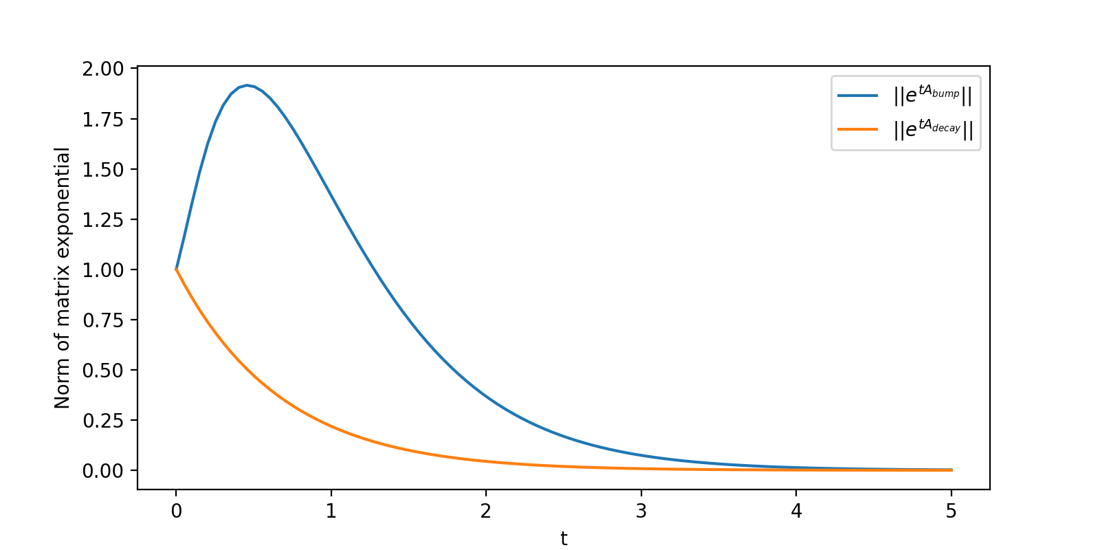
Figure 2: Plot of $||e^{tA_{\text{bump}}}||$ and $||e^{tA_{\text{decay}}}||$ versus time $t$. Blue curve corresponds to positive $\gamma$ defined in equation (20b) and the orange corresponds to negative $\gamma$.

For our experiments, we consider $A=A_{\text{bump}}$. and $\epsilon\in\{0,1.0\}$. The initial bump in the norm $||e^{tA_{\text{bump}}}||$ makes the dynamics more challenging to learn, as this implies initial transient growth before the long term decay. Data is generated using an adaptive Runge-Kutta-Fehlberg scheme. There are 1000 initial conditions evolved using 50 adaptive timesteps and a relative tolerance of $10^{-8}$. For $\epsilon=0.0$ two large timesteps are taken and for $\epsilon=1.0$ there are 5 large timesteps. Note that the exponential integrator can learn the dynamics for $\epsilon=0.0$ with a single timestep, but the IMEX scheme is unable to capture the dynamics. In our network, the nonlinear term is treated using a bilinear form network when $\epsilon=0.0$ and Lipschitz controlled layers when $\epsilon=1.0$. In both cases 2 layers and 100 hidden dimensions are used. The Adam optimizer from Optax is used for training with a learning rate of 0.01 and batch size of 1000. The training is run for 1000 iterations for each case. For comparison, an implicit-explicit (IMEX) scheme is used with the same training parameters. The predictions of the models for $\epsilon=0.0$ are shown in Figure 3 and for $\epsilon=1.0$ are shown in Figure 4. Learning with the exponential integrator yields more accurate results than the IMEX integrator for both values of $\epsilon$, the difference is more pronounced for the $\epsilon=1.0$.

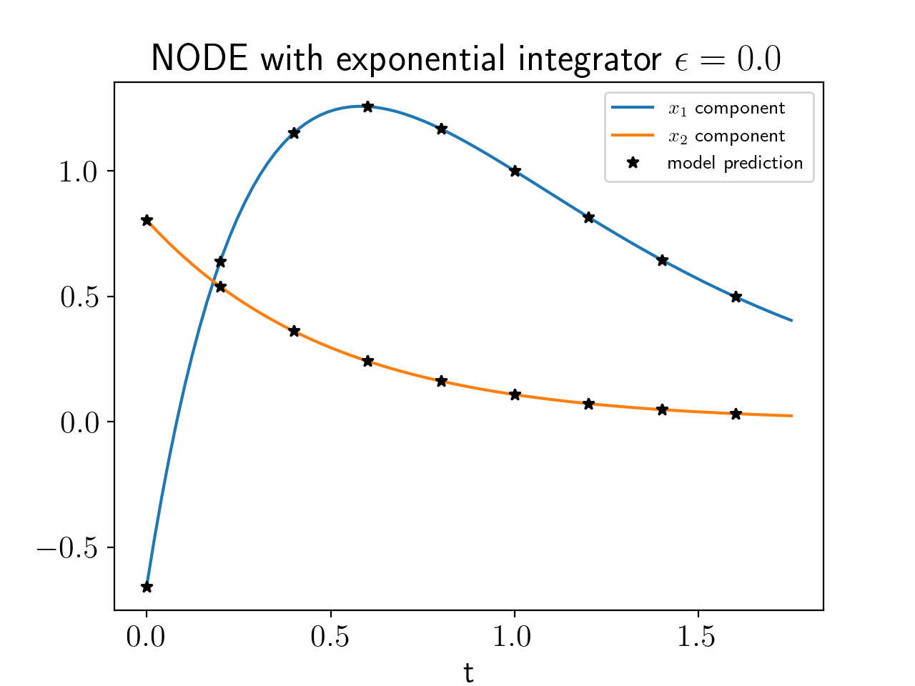
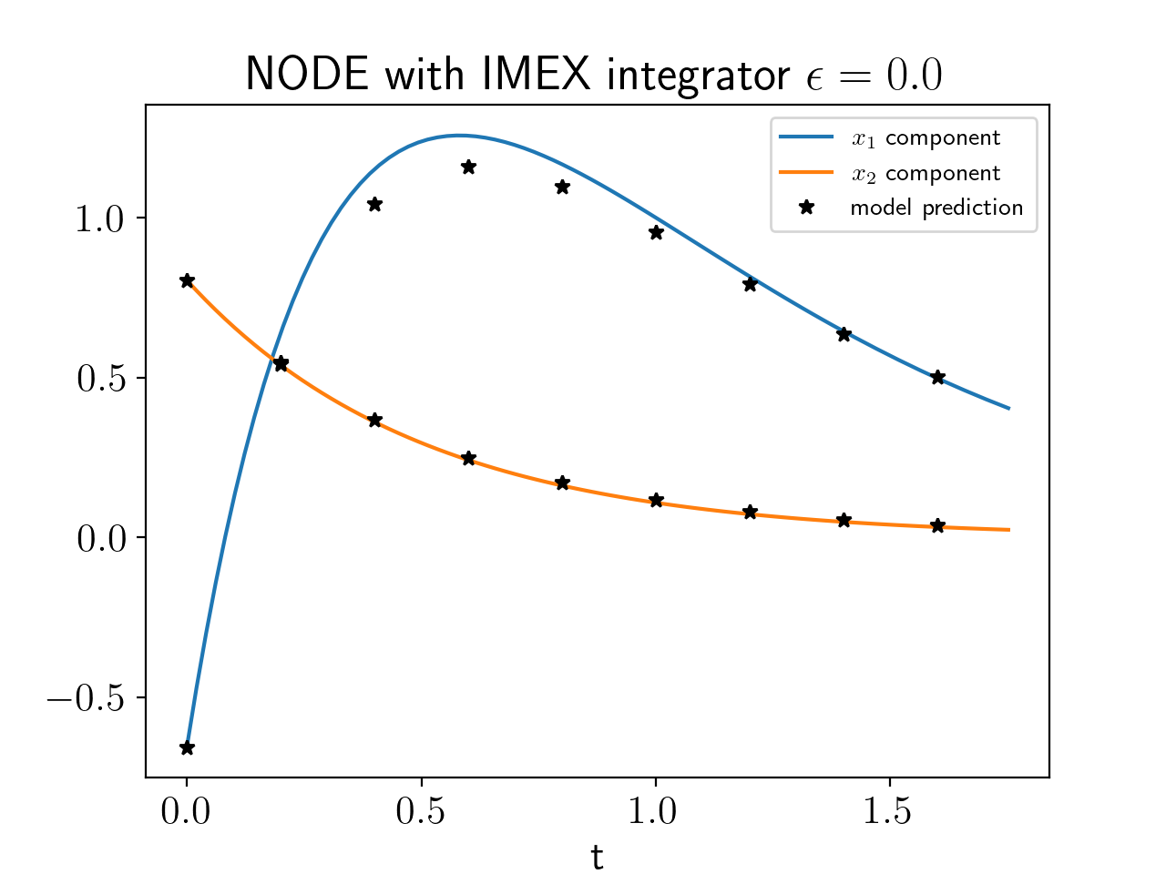
Figure 3: Prediction of the weakly nonlinear system using and exponential integrator (Left) and and IMEX integrator (Right) using two large timesteps and a bilinear form for the nonlinear term. Black dots represent the model prediction using timesteps of $\Delta t=0.2$. The blue and orange curves represents the true dynamics for $x_{1}$ and $x_{2}$, respectively.

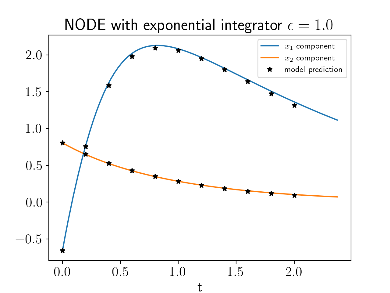
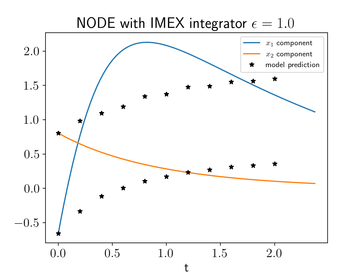
Figure 4: Prediction of the weakly nonlienar system with $\alpha=1.0$ using an exponential integrator (Left) and an IMEX integrator (Right) using five timesteps and Lipschitz controlled neural network for the nonlinear term. Black dots represent the model prediction using timesteps of $\Delta t=0.2$ . The blue and orange curves represents the true dynamics for $x_{1}$ and $x_{2}$, respectively.

5.2 Grad-13

We consider a linear Grad-13 moment system

(22) $$\partial_{t}\rho =-\epsilon\,\nabla\cdot\mathbf{u},$$

(23) $$\partial_{t}\mathbf{u} =-\epsilon\left(\nabla\rho+\nabla T+\nabla\cdot\sigma\right),$$

(24) $$\partial_{t}T =-\frac{2\epsilon}{3}\left(\nabla\cdot\mathbf{u}+\nabla\cdot\mathbf{q}\right),$$

(25) $$\partial_{t}\mathbf{\sigma} =-\mathbf{\sigma}-\epsilon\left(2\overline{\nabla\mathbf{u}}+\frac{4}{5}\overline{\nabla\mathbf{q}}\right),$$

(26) $$\partial_{t}\mathbf{q} =-\frac{2}{3}\mathbf{q}-\epsilon\left(\frac{5}{2}\nabla T+\mathbf{\nabla}\cdot\mathbf{\sigma}\right),$$

where $\rho(\mathbf{x},t)$ is the density, $\mathbf{u}(\mathbf{x},t)$ is velocity, $T(\mathbf{x},t)$ is temperature, $\sigma(\mathbf{x},t)$ is the stress tensor, $\mathbf{q}(\mathbf{x},t)$ is the heat flux, and $\mathbf{x}=(x,y,z)^{T}\in\mathbb{R}^{3}$ is the spatial coordinate. The overline represents the symmetric, traceless part of a tensor, e.g.

(27) $$\overline{\mathbf{a}} =\frac{1}{2}(\mathbf{a}+\mathbf{a}^{T})-\frac{1}{3}\mathbf{I}\,\text{Tr}(\mathbf{a}).$$

We consider solutions that are one-dimensional ($\partial_{y}=\partial_{z}=0$) and $2\pi$-periodic in space, e.g.

(28) $$\rho(\mathbf{x},t)=\sum_{k=-\infty}^{\infty}\rho_{k}(t)e^{ikx}.$$

The Fourier coefficients are governed by the following system of ODEs.

(44) $$\frac{d}{dt}\left[\begin{array}[]{c}\rho_{k}\\ u_{k}\\ T_{k}\\ \sigma_{k}\\ q_{k}\end{array}\right]=\left[\begin{array}[]{ccccc}0&-ik\epsilon&0&0&0\\ -ik\epsilon&0&-ik\epsilon&-ik\epsilon&0\\ 0&-\frac{2}{3}ik\epsilon&0&0&-\frac{2}{3}ik\epsilon\\ 0&-\frac{4}{3}ik\epsilon&0&-1&-\frac{8}{15}ik\epsilon\\ 0&0&-\frac{5}{2}ik\epsilon&-ik\epsilon&-\frac{2}{3}\end{array}\right]\left[\begin{array}[]{c}\rho_{k}\\ u_{k}\\ T_{k}\\ \sigma_{k}\\ q_{k}\end{array}\right],\quad k=0,\pm 1,\dots$$

For this example, we truncate the Fourier series to include the $k=0,\pm 1,\pm 2$ modes. $\epsilon$ is fixed at $\epsilon=0.1$ and 1000 initial trajectories generated uniformly from the complex region $[-1,1]\times[-i,i]$. The initial conditions are evolved by taking 10 evenly spaced timesteps from time $t_{0}=0$ to $t_{f}=4$. These trajectories are used for training. A stucture-preserving NODE is trained using the Adam optimizer from Optax. The learning rate is set to 0.005 and batch size is 100. The linear part is parameterized using the Hurwitz decompostion and the nonlinear part is parameterized using a Lipschitz controlled feed forward neural network with one layer and 5 hidden dimensions.

Figure 5 shows the comparison of the trained model and a reference solution computed out to final time 80 which is 20 times longer than the training data.

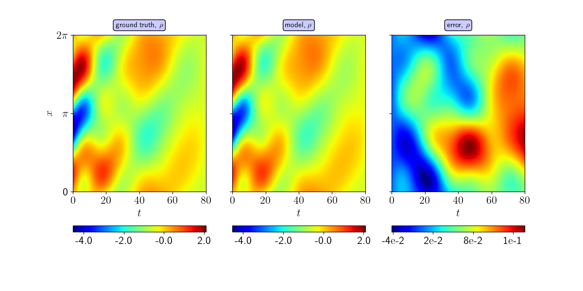
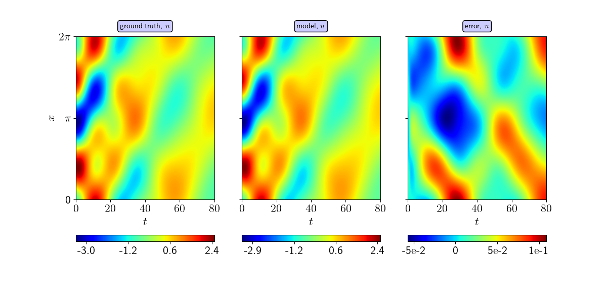
Figure 5: Comparison of slow scale variables (Top) density, (middle) velocity and (bottom) Temperature.

5.3 Kuramoto-Sivashinsky Equation

In this section we consider the one-dimensional Kuramoto-Sivashinsky (KS) equation

(45) $$\frac{du}{dt}=-u\frac{du}{dx}-\frac{d^{2}u}{dx^{2}}-\frac{d^{4}u}{dx^{4}},$$

with periodic boundary conditions on a domain of length $L=22$. The KS equation exhibits chaotic behavior; therefore, we do not expect pointwise accuracy in the long term. To check the validity of our solution we rely on statistical measures, namely, the probability distribution function of the first and the second spatial derivatives, $u_{x}$ and $u_{xx}$.

We consider the dataset used in [17]. Solutions are found by performing a Galerkin projection onto Fourier modes and using exponential time differencing to evolve the ODE forward in time [12]. After solving in Fourier space, we then transform the data back to physical space for training the neural ODEs. We sample the data at every 1.0 time units. The training data is constructed by separating the long trajectory into trajectories with 8 steps. Our batch size is 2000 and our learning rate is 0.001. The learning rate is reduced by a factor of 0.99 at each step. For this problem we use a Lipschitz controlled feed-forward neural network for the nonlinear part using 2 layers and inner dimension 200. We observe that Lipschitz control simultaneously improves training performance and the long-term stability of the dynamic model.

There are a few additional steps taken to train this model effectively. First, a shift of the spectrum to the Hurwitz matrix is applied during training. This is required since the KS system has both positive and negative eigenvalues and the Hurwitz parametrization requires the real part of the eigenvalues to be negative. Second, an autoencoder that projects the dynamics down to a latent space. There are many attractive options for model reduction. A popular method is utilizing projection based reduced-order modeling, which attempt to find a low-dimensional trial subspace that can represent the state space. Most of these trial subspaces are linear and can not capture the complicated dynamics of the KS equation. Moreover, the KS equation has a slow decaying Kolomogorov $n$-width [20], which implies linear trial subspaces may not accurately represent the system. The power behind autoencoders is that they attempt to find an identity mapping with fewer dimensions. If the data can be represented in a lower dimensional nonlinear manifold, then optimization of the encoder and decoder finds the optimal low-order representation. For this example 64 grid points are projected into a latent space of size 20 using an autoencoder.

In Figure 6 the evolution of the true solution (Top), model (Middle) and error (Bottom) are displayed until time $t=200$. The dynamics agree pointwise until around time $t=50$ after which we must rely on other measures to assess the validity of the model.

To verify the long-time behavior of predicting this chaotic system, Figure 7 presents the joint probability distribution function of $u_{x}$ and $u_{xx}$. Qualitatively they match well demonstrating that the statistics of the dynamics agree between the model and the ground truth.

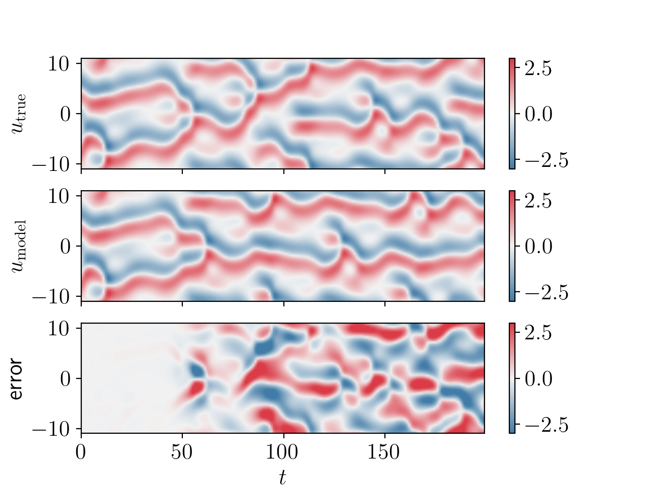
Figure 6: Displayed is the true solution (Top), the model prediction (Middle) and the error (Bottom). The agreement between the true solution and the model holds until $t=50$ then the chaotic nature of KS makes it difficult for our model to be pointwise accurate.

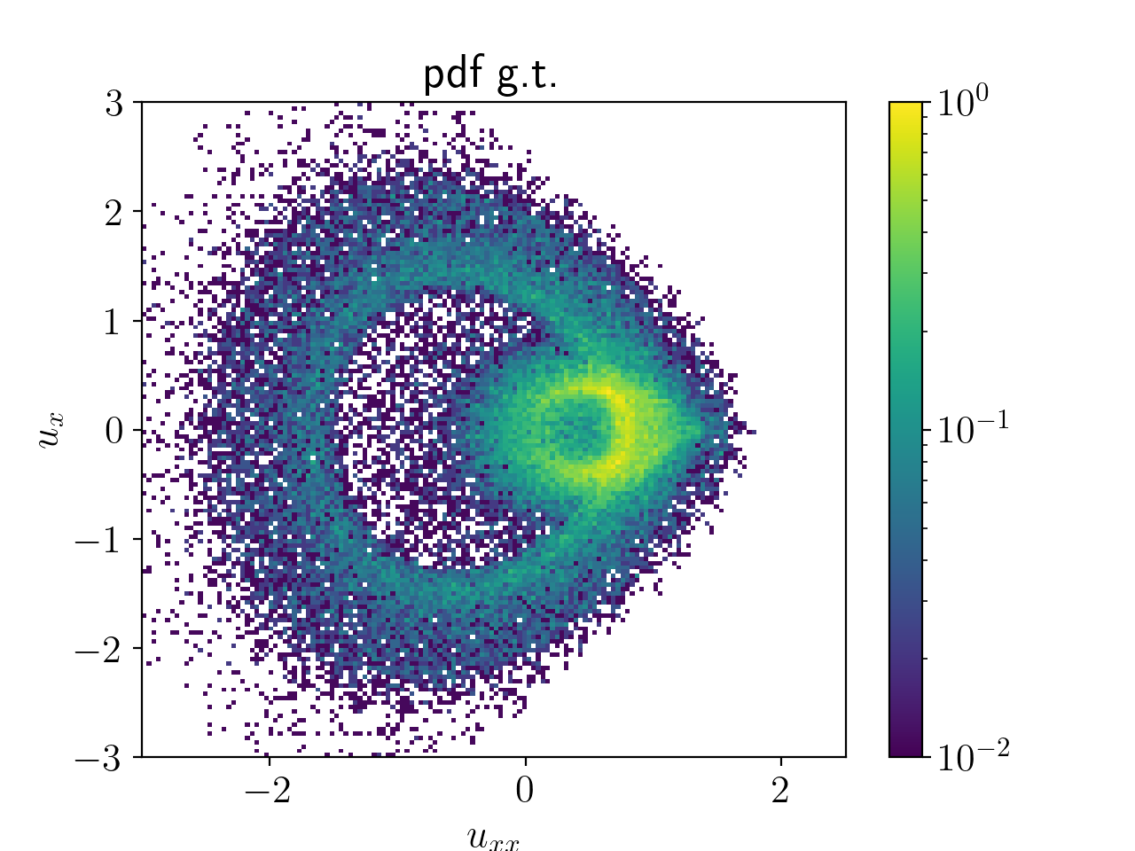
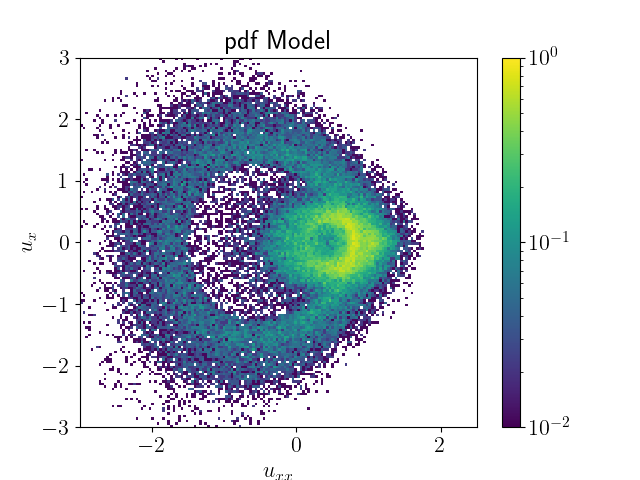
Figure 7: The joint probability distribution function of $u_{x}$ and $u_{xx}$ is displayed for the ground truth (Left) and the model (Right).

6 Conclusions

This work presents a novel approach to addressing the long-term stability issues of neural ordinary differential equations (NODEs), a crucial aspect for efficient and robust modeling of dynamical systems. By combining a structure-preserving NODE with a linear and nonlinear split, an exponential integrator, constraints on the linear operator through Hurwitz matrix decomposition, and a Lipschitz-controlled neural network for the nonlinear operator, the proposed approach demonstrates significant advantages in both learning and deployment over standard explicit and implicit NODE methods. This approach enables the efficient modeling of complex stiff systems and provides a stable foundation for deploying NODE models in real-world applications. We demonstrate our approach in various examples. For the weakly nonlinear ODE example, we show that using an exponential integrator provides significant accuracy over a semi-implicit scheme. We also demonstrate the structure-preserving NODE approach in time dependent PDEs, such as the Grad-13 and Kuramoto-Sivashinksy systems, showcasing its ability to learn both multi-scale and chaotic systems.

References

- [1] A. H. Al-Mohy and N. J. Higham, Computing the action of the matrix exponential, with an application to exponential integrators, SIAM journal on scientific computing, 33 (2011), pp. 488–511.
- [2] J. Bradbury, R. Frostig, P. Hawkins, M. J. Johnson, C. Leary, D. Maclaurin, G. Necula, A. Paszke, J. VanderPlas, S. Wanderman-Milne, and Q. Zhang, JAX: composable transformations of Python+NumPy programs, 2018.
- [3] R. T. Chen, Y. Rubanova, J. Bettencourt, and D. K. Duvenaud, Neural ordinary differential equations, Advances in neural information processing systems, 31 (2018).
- [4] DeepMind, I. Babuschkin, K. Baumli, A. Bell, S. Bhupatiraju, J. Bruce, P. Buchlovsky, D. Budden, T. Cai, A. Clark, I. Danihelka, A. Dedieu, C. Fantacci, J. Godwin, C. Jones, R. Hemsley, T. Hennigan, M. Hessel, S. Hou, S. Kapturowski, T. Keck, I. Kemaev, M. King, M. Kunesch, L. Martens, H. Merzic, V. Mikulik, T. Norman, G. Papamakarios, J. Quan, R. Ring, F. Ruiz, A. Sanchez, L. Sartran, R. Schneider, E. Sezener, S. Spencer, S. Srinivasan, M. Stanojević, W. Stokowiec, L. Wang, G. Zhou, and F. Viola, The DeepMind JAX Ecosystem, 2020.
- [5] G.-R. Duan and R. J. Patton, A note on Hurwitz stability of matrices, Automatica, 34 (1998), pp. 509–511.
- [6] W. D. Fries, X. He, and Y. Choi, LASDI: Parametric latent space dynamics identification, Computer Methods in Applied Mechanics and Engineering, 399 (2022), p. 115436.
- [7] C. Fronk and L. Petzold, Training stiff neural ordinary differential equations with explicit exponential integration methods, arXiv preprint arXiv:2412.01181, (2024).
- [8] N. J. Higham, Accuracy and stability of numerical algorithms, SIAM, 2002.
- [9] N. J. Higham, The scaling and squaring method for the matrix exponential revisited, SIAM Journal on Matrix Analysis and Applications, 26 (2005), pp. 1179–1193.
- [10] M. Hochbruck, C. Lubich, and H. Selhofer, Exponential integrators for large systems of differential equations, SIAM Journal on Scientific Computing, 19 (1998), pp. 1552–1574.
- [11] M. Hochbruck and A. Ostermann, Exponential integrators, Acta Numerica, 19 (2010), pp. 209–286.
- [12] A.-K. Kassam and L. N. Trefethen, Fourth-order time-stepping for stiff pdes, SIAM Journal on Scientific Computing, 26 (2005), pp. 1214–1233.
- [13] P. Kidger, On Neural Differential Equations, PhD thesis, University of Oxford, 2021.
- [14] S. Kim, W. Ji, S. Deng, Y. Ma, and C. Rackauckas, Stiff neural ordinary differential equations, Chaos: An Interdisciplinary Journal of Nonlinear Science, 31 (2021).
- [15] H. Krovi, Improved quantum algorithms for linear and nonlinear differential equations, Quantum, 7 (2023), p. 913.
- [16] M. Lienen and S. Günnemann, torchode: A parallel ODE solver for PyTorch, in The Symbiosis of Deep Learning and Differential Equations II, NeurIPS, 2022.
- [17] A. J. Linot, J. W. Burby, Q. Tang, P. Balaprakash, M. D. Graham, and R. Maulik, Stabilized neural ordinary differential equations for long-time forecasting of dynamical systems, Journal of Computational Physics, 474 (2023), p. 111838.
- [18] Y. Y. Lu, Computing a matrix function for exponential integrators, Journal of computational and applied mathematics, 161 (2003), pp. 203–216.
- [19] B. Lusch, J. N. Kutz, and S. L. Brunton, Deep learning for universal linear embeddings of nonlinear dynamics, Nature communications, 9 (2018), p. 4950.
- [20] R. Mojgani, M. Balajewicz, and P. Hassanzadeh, Kolmogorov n–width and Lagrangian physics-informed neural networks: A causality-conforming manifold for convection-dominated pdes, Computer Methods in Applied Mechanics and Engineering, 404 (2023), p. 115810.
- [21] D. A. Serino, A. A. Loya, J. Burby, I. G. Kevrekidis, and Q. Tang, Intelligent attractors for singularly perturbed dynamical systems, arXiv preprint arXiv:2402.15839, (2024).
- [22] X. Xie, Q. Tang, and X. Tang, Latent space dynamics learning for stiff collisional-radiative models, Machine Learning: Science and Technology, 5 (2024), p. 045070.
- [23] H. Zhang, Y. Liu, and R. Maulik, Semi-implicit neural ordinary differential equations for learning chaotic systems, in NeurIPS 2023 Workshop Heavy Tails in Machine Learning, 2023.
- [24] H. Zhang, Y. Liu, and R. Maulik, Semi-implicit neural ordinary differential equations, arXiv preprint arXiv:2412.11301, (2024).