Noisy-enhanced quantum search on complex networks

Abstract

The task of finding an element in an unstructured database is known as spatial search and can be expressed as a quantum walk evolution on a graph. In this article, we modify the usual search problem by adding an extra trapping vertex to the graph, which is only connected to the target element. The walker evolution is a mix between classical and quantum walk search dynamics. The balance between unitary and non-unitary dynamics is tuned with a parameter, and we numerically show that depending on the graph topology and the connectivity of the target element, this hybrid approach can outperform a purely classical or quantum evolution for reaching the trapping site. We show that this behavior is only observed in the presence of an extra trapping site, and that depending on the topology, the increase of non-unitary operations can be compensated by increasing the strength of the quantum walk exploration. This compensation comes at the cost of reducing the searching feature of the evolution induced by the Hamiltonian. We also relate the optimal hybrid regime to the entropy’s decay rate. As the introduction of non-unitary operations may be considered as noise, we interpret this phenomena as a noisy-assisted quantum evolution.

I Introduction

Quantum walks are the quantum analog of random walks. They are a coherent model of transportation on graphs and a universal model of quantum computation [1, 2], formulated both in continuous and discrete-time. Continuous-time quantum walks (CTQWs) evolve on the space spanned by the vertices of a graph whose structure is encoded in an Hamiltonian [3]. As for discrete-time quantum walks (DTQWs), they require the use of a coin to guide the displacements, which enlarges the Hilbert space of the system [4]. Both formalisms are fundamental quantum computing tools as they serve for quantum simulation of fundamental physics [5, 6, 7, 8, 9] and quantum field theory [10, 11, 12], quantum information processing and quantum algorithms [13, 14]. Among their algorithmic applications, few examples are related to optimization problems [15, 16, 17, 18, 19, 20], quantum state preparation [21, 22, 23], machine learning tasks [24, 25, 26, 27] or graph related problems [28, 29, 30]. Moreover, it has been proved that some DTQWs converge to the Dirac [31, 32, 33, 34, 35] and the Schrödinger [36] equations in their continuous limit.

The task of finding a marked element in an unstructured database is known as spatial search. Naturally, the database is modeled as a graph whose vertices and edges respectively represent its elements and their relationships. The most famous related result is Grover’s algorithm [37] which requires $\mathcal{O}(\sqrt{N})$ calls to an oracle to find an element among $N$ in an unstructured database. This algorithm is optimal if the oracle is given as a black box [38] and was surprisingly shown to be a naturally occurring phenomenon [39]. However, when the inner structure of the oracle is known, a classical quantum-inspired algorithm can potentially solve the search problem exponentially faster by simulating the oracle several times [40]. The associated complexity depends on the cost of a single simulation. Moreover, the search problem can be expressed as a quantum walk evolution on graphs, both in discrete [41] and continuous-time [42], each resulting in a quadratic speedup on arbitrary graphs [43, 44].

Quantum walks in open quantum system can be modeled by Quantum Stochastic Walks (QSWs), which are a generalization of CTRWs and CTQWs [45]. They were first introduced as a tool to study the transition between classical and quantum random walks. QSWs have been proposed as an algorithmic tool for several problems including PageRank [46], decision-making [47], quantum state discrimination [48], or function approximation and classification [49]. A discrete-time QSW scheme has also been proposed by Schuhmacher et al. [50]. QSWs have been accurately produced experimentally with a three-dimensional photonic quantum chip [51] and could generally be implemented with the method proposed by Ding et al. for simulation of open quantum systems [52]. Using the QSWs framework, Caruso has numerically shown that for several graphs, transfer efficiency from an arbitrary vertex to an absorbing vertex, named the sink, is optimal when dynamics is 90% coherent and 10% incoherent [53]. Moreover, Caruso et al. have experimentally implemented a photonic maze from which a single photon must escape, and they recovered the same result: the walker finds his way out faster to the sink when 10% of the dynamics is non-unitary [54]. These results suggests that a controlled amount of non-unitary dynamics, which may be interpreted as noise, can improve transfer efficiency from an arbitrary set of vertices to a sink. Lastly, maze solving in open quantum systems has also been studied with QSWs assisted by reinforcement learning [55] or with a Grover walk that makes use of sink vertices [56].

In this article, we use continuous-time dynamics to tackle a modified version of the search problem for single marked element. We introduce the Stochastic Quantum Walk Search (SQWS) monitored by a weighted Lindbladian. The unitary evolution is induced by Childs and Goldstone’s CTQW search Hamiltonian [42], and non-unitary dissipation is designed to implement a CTRW search dynamics. In addition, we use a trapping sink vertex as an extra dissipative tool, which we only connect to the target vertex of the search with an irreversible transition. The walker starts from a uniform superposition over the vertices of the graph and has to reach the trapping site by moving through a search-driven dynamics guiding it to the target vertex. We numerically show that a mix of unitary and non-unitary operations can outperform a fully coherent or incoherent dynamics for reaching the sink. The balance between unitary and non-unitary operations is controlled with a tunable mixing parameter. The performance of the hybrid regime depends on the graph topology and the connectivity of the target vertex. We show that an increase of non-unitary operations may be compensated by increasing the strength of the quantum walk exploration, at the cost of reducing the importance of the searching oracle that marks the target vertex. Moreover, we show that the addition of non-unitary operations leads to an improvement of performance only in the presence of a sink. Lastly, we relate the best mixing parameter of unitary and non-unitary dynamics to the system’s entropy decay rate. We interpret the hybrid regime as a noisy-assisted quantum evolution as it contains non-unitary operations, even if does not model realistic hardware noise.

We start by introducing different continuous-time dynamics on graphs and the search problem of a single element in Sec. II. We present our model for the modified version of the search problem and our results in Sec. III.

II Preliminaries

II.1 Continuous-time dynamics

II.1.1 Random Walks

Continuous-time Random Walks (CTRWs) describe the evolution of a single walker on a network modeled by a graph $G=(V,E)$ where $V$ and $E$ are respectively a set of vertices and edges. An unweighted graph is fully described by its adjacency matrix:

$$A_{ij}=\begin{cases}1\text{ if }(i,j)\in E,\\ 0\text{ otherwise}.\end{cases}$$ (1)

The CTRW is a Markov process whose rate matrix is the Laplacian $L=D-A$ of the graph, with $D$ a matrix whose diagonal entries are the degree of each vertex. The state of the walker is described by a probability distribution $\vec{p}$ which is a map from $V$ to probabilities. The time evolution of the walker is:

$$\frac{d}{dt}\vec{p}(t)=-L\vec{p}(t).$$ (2)

As the column of $L$ sum to zero, an initially normalized probability distribution remains valid under the evolution induced by Eq. (2).

II.1.2 Quantum Walks

Continuous-time quantum walks are a coherent model of transportation over complex networks [57]. The walker is represented with a quantum state $\ket{\psi}$ that evolves in an Hilbert space $\mathcal{H}$ spanned by the vertices of the graph. Therefore, the set of vertices $V$ form an orthonormal basis of $\mathcal{H}$. The time evolution of the walker is given by the Schrödinger equation and the Hamiltonian encodes the structure of the graph:

$$i\hbar\frac{d}{dt}\ket{\psi(t)}=H\ket{\psi(t)}.$$ (3)

Throughout, we work in units in which $\hbar=1$. As the evolution is unitary, the Hamiltonian $H$ has to be Hermitian, making the underlying graph undirected, which is not the case for CTRWs as their underlying graph can have both directed and undirected edges.

II.1.3 Quantum Stochastic Walks

The transition from the classical to the quantum regime can be studied with the QSW framework that enables to interpolate between coherent and incoherent dynamics [45]. The state of the walker is described by a density matrix $\rho=\ket{\psi}\bra{\psi}$ as the evolution is composed of both unitary and non-unitary operations. The QSWs evolution is driven by a weighted Lindblad master equation with $\omega\in[0,1]$:

$$\small{\begin{split}\frac{d}{dt}\rho(t)&=-i(1\!-\!\omega)[H,\rho(t)]\!+\!\omega\!\sum_{ij}\!\Big{(}\!\mathcal{L}_{ij}\rho(t)\mathcal{L}_{ij}^{\dagger}\!-\!\frac{1}{2}\!\{\!\mathcal{L}_{ij}^{\dagger}\mathcal{L}_{ij},\rho(t)\!\}\!\Big{)}\\ &=(1-\omega)\mathcal{U}_{H}[\rho(t)]+\omega\mathcal{D_{L}}[\rho(t)],\end{split}}$$ (4)

where $[\alpha,\beta]=\alpha\beta-\beta\alpha$ and $\{\alpha,\beta\}=\alpha\beta+\beta\alpha$ are the commutator and anti-commutator of operators $\alpha$ and $\beta$. The unitary and non-unitary dynamics are respectively encapsulated by $\mathcal{U}_{H}$ and $\mathcal{D_{L}}$, and the parameter $\omega$ enables to interpolate between them. A wise choice of Lindblad jump operators $\mathcal{L}_{ij}$ can describe a CTRW evolution [45]. Therefore, for well-defined Lindblad jump operators, the CTQW is recovered for $\omega=0$ and the CTRW for $\omega=1$. A linear combination of the two is obtained for other values of $\omega$, leading to a mix between coherent and incoherent dynamics for the walker. It was shown that the introduction of an extra sink vertex in Eq. (4), with $H=A$ and $\mathcal{L}_{ij}=A_{ij}/D_{ij}\ket{i}\bra{j}$, leads to an optimal transfer from a set of vertices to this sink vertex when $\omega=0.1$ for several graphs [53].

II.2 Spatial Search

II.2.1 Random Walk Search

Spatial search expressed as a CTRW evolution consists of a walker spreading over the vertices of a graph until it reaches the marked element $m$. The marked vertex is an absorbing vertex, meaning that the probability of leaving it is zero. Therefore, the Laplacian has to be modified into an absorbing Laplacian $\hat{L}=\frac{D-\hat{A}}{||D-\hat{A}||_{2}}$ where $\hat{A}$ is the adjacency matrix whose $m$-th column is the $m$-th canonical basis vector of $\mathbb{R}^{|V|}$ [58]. The initial state is the uniform probability distribution over the vertices of the graph:

$$\vec{p}(0)=\frac{1}{|V|}\sum_{v\in V}\vec{e}_{v},$$ (5)

where $\{\vec{e}_{v}|v\in V\}$ is the set of canonical basis vectors of $\mathbb{R}^{|V|}$.

II.2.2 Quantum Walk Search

An optimal quantum walk search algorithm on arbitrary graphs has been introduced by Apers et al. [44]. However, their algorithm implies an expansion of system’s Hilbert space as their evolution requires the preparation of an auxiliary Gaussian state. As we do not want to increase the size of the Hilbert space, we use the Hamiltonian introduced by Childs and Goldstone that allows an evolution in the space spanned by the vertices of the graph, even if this framework is not optimal for all graphs [42]. Thus, the search Hamiltonian is defined as:

$$H_{m,\gamma}=\gamma L-\ket{m}\bra{m},$$ (6)

where $\gamma\in\mathbb{R}^{+}$ determines the strength of the interaction between the walker’s quantum dynamics on the graph and the marked vertex respectively induced by the Laplacian $L$ and the oracle $\ket{m}\bra{m}$. The initial state is the uniform superposition over the vertices of the graph:

$$\ket{\psi(0)}=\frac{1}{\sqrt{|V|}}\sum_{v\in V}\ket{v}.$$ (7)

The heart of the CTQWs spatial search algorithm is to find the minimal value of $t$ and the optimal value of $\gamma$ to maximize the success probability $|\bra{m}e^{-itH_{m,\gamma}}\ket{\psi(0)}|^{2}$ of finding the marked element. This algorithm was first shown to offer a quadratic speedup over its classical counterparts for the complete graph, the hypercube and the $d$-dimensional periodic lattice for $d>4$ [42], and to be optimal for a wide family of graphs by Chakraborty et al. [59]. Lastly, it was shown that quantum walk search performances in this framework can be predicted if certain conditions on the spectral properties of the Hamiltonian driving the walk are met [60].

III Results

III.1 Stochastic Quantum Walk Search

III.1.1 Model

The SQWS is composed of CTQW and CTRW search dynamics with an additional sink. The sink plays a fundamental role in the system, as we later show that the introduction of non-unitary dynamics improves performance only in its presence. We introduce the sink vertex $\phi$ and connect it to the target vertex $m$. The irreversible transition from $m$ to $\phi$ is modeled by the Lindblad jump operator:

$$\mathcal{L}_{\phi,m}[\rho(t)]=\ket{\phi}\bra{m}\rho(t)\ket{m}\bra{\phi}-\frac{1}{2}\{\ket{m}\bra{m},\rho(t)\}.$$ (8)

Therefore, the evolution of the SQWS is:

$$\begin{split}\frac{d}{dt}\rho(t)&=(1-\omega)\mathcal{U}_{H_{m,\gamma}}[\rho(t)]+\omega\mathcal{D}_{\mathcal{L}}[\rho(t)]+\Gamma\mathcal{L}_{\phi,m}[\rho(t)]\\ &=\mathcal{E}[\rho(t)],\end{split}$$ (9)

with $\Gamma\in\mathbb{R}^{+}$ the sink rate and $\mathcal{L}_{ij}=-\hat{L}_{ij}\ket{i}\bra{j}$. Thus, the coherent and incoherent dynamics respectively produce a quantum and classical random walks search. The initial state is the uniform superposition over the vertices of the graph (excluding the sink vertex) $\rho(0)=\ket{\psi(0)}\bra{\psi(0)}$. As an illustration, we show in Fig. 1 a graph with the extra sink vertex $\phi$ connected to the target vertex $m$.

In this article, we study the transfer efficiency from an uniform superposition over the vertices to the sink. The walker is guided to the target vertex with a search Hamiltonian, and non-unitary operations designed to implement a CTRW-search, which we interpret as noise. Once on the target vertex, the walker may jump to the sink and remains trapped inside. We find the optimal value of $\gamma$ with a classical optimizer when $\omega<1$ in the spirit of Ref. [61]. Starting from a uniform superposition over the vertices, we aim at maximizing the transfer efficiency to the sink (connected only to the marked vertex). Thus, the cost function associated with the optimization of $\gamma$ is:

$$E_{\omega,t}(\gamma)=\frac{1}{t}\int_{0}^{t}\text{Tr}\left({\mathcal{E}[\rho(\tau)]\ket{\phi}\bra{\phi}}\right)\,\text{d}\tau.$$ (10)

We normalize Eq. (10) so that $E_{\omega,t}(\gamma)=1$ corresponds to a total instantaneous transfer of the walker to the sink vertex, and $E_{\omega,t}(\gamma)=0$ that its probability of presence on the sink is zero. As, Eq. (10) considers both success probability and its associated evolution time, it is our unique performance metric. Moreover, we have also executed the SQWS with no sink and show that its presence is mandatory for the hybrid dynamics to beat a fully classical or quantum dynamics. In the absence of sink, the introduction of non-unitary dynamics always reduces performance as we show in Appendix A.

Figure 1: Modified cycle graph $C_{6}$ on which we add the extra sink vertex $\phi$ connected to the target vertex $m$. The irreversible transition from $m$ to $\phi$ is weighted with the sink rate $\Gamma$. The classical and quantum walk search dynamics only act on the vertices of the initial graph, not on the sink vertex. The search dynamics guides the walker to the target vertex $m$ for it to reach the sink $\phi$, and “escape” the graph.

III.1.2 Numerical results

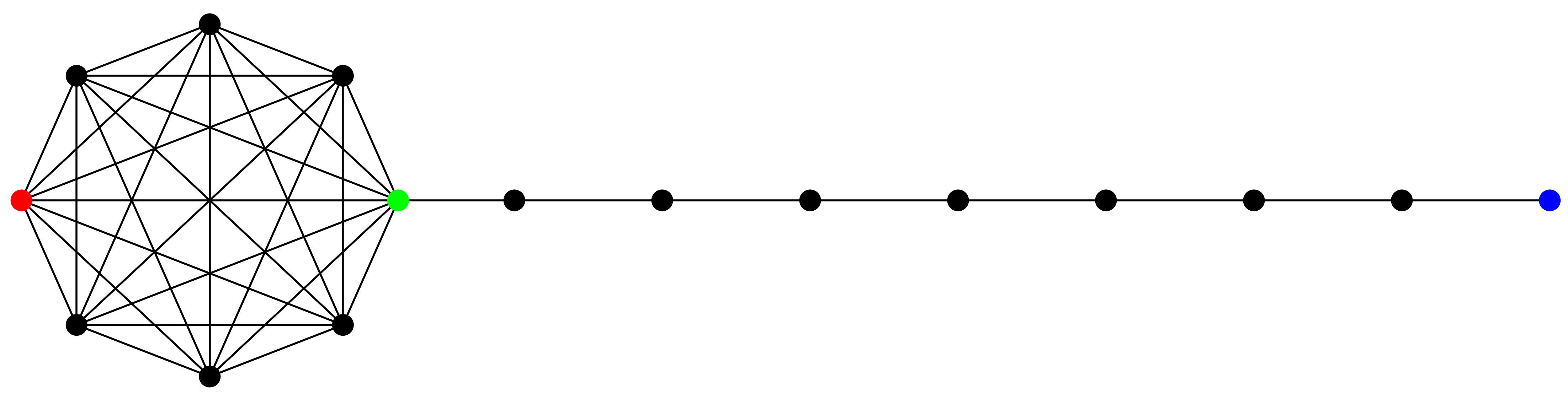
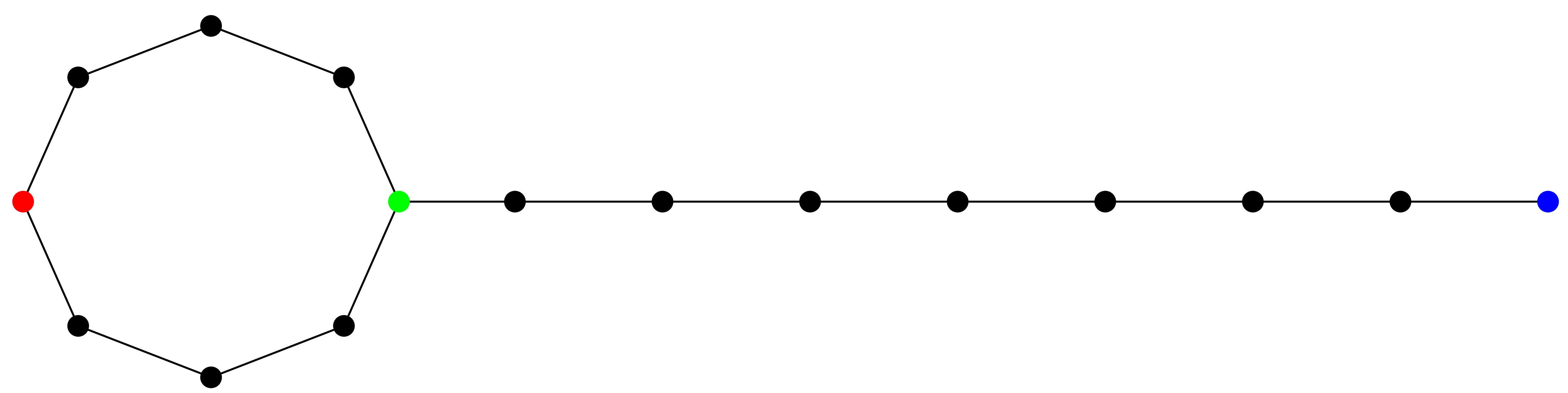
Figure 3: Instances $L_{8,8}$ and $T_{8,8}$ of the lollipop (upper) and tadpole (lower) graphs, that are respectively a fusion between the complete graph $K_{8}$ or the cycle graph $C_{8}$ with the path graph $P_{8}$. We respectively refer to the locations of the red, green and blue vertices as complete, shared and path vertices for the lollipop graph, and cycle, shared and path for the tadpole graph.

We run the SQWS on instances of different graph families and show the results in Fig. 2. The simulation parameters are set to $\Gamma=1$ and $t=10|V|$. We set the time to be linear with the size of the graph as we mentioned that the sink removes any potential quadratic speedup. The classical optimization of $\gamma$ is done with Simulated Annealing [62]. For each graph, we set bounds on the maximum achievable value for the optimization of $\gamma$ to see the impact of its increase on performance. This parameter in the Hamiltonian controls the balance between the exploration of the graph and its interaction with the target vertex. We also point out that as the value of $\gamma$ increases, the graph exploration induced by the Laplacian in the Hamiltonian of Eq. (6) will predominate over the oracle marking the target vertex connected to the sink. Therefore, we run the SQWS with the bounds $\gamma\in[0,\gamma_{\max}]$ for $\gamma_{\max}\in\{1,2,4,6,8,10,15,20,30,40,50,60,70,80,90,100,4|V|\}$. We present the main results in Fig. 2 which illustrates the execution of the SQWS on the complete graph $K_{64}$, the 6-dimensional hypercube $Q_{6}$, the cycle graph $C_{64}$, the lollipop graph $L_{32,32}$ and the tadpole graph $T_{32,32}$. The lollipop $L_{M,N}$ and tadpole $T_{M,N}$ graphs are respectively the fusion between a complete or cycle graph of size $M$ with a path of size $N$, we display two instances of these graphs in Fig. 3.

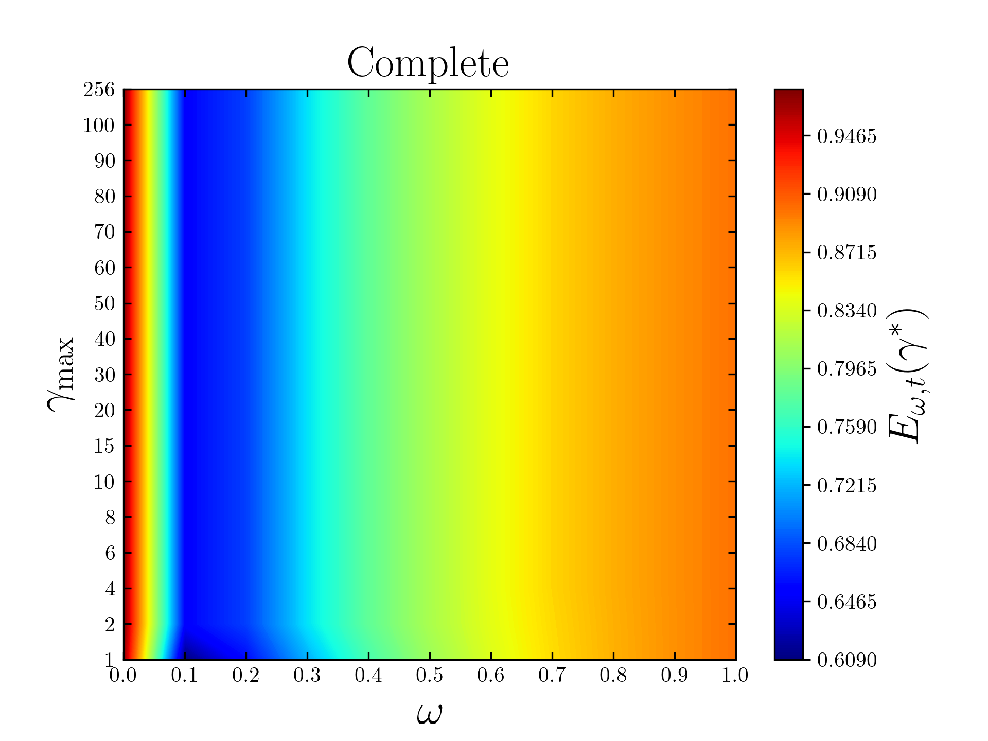
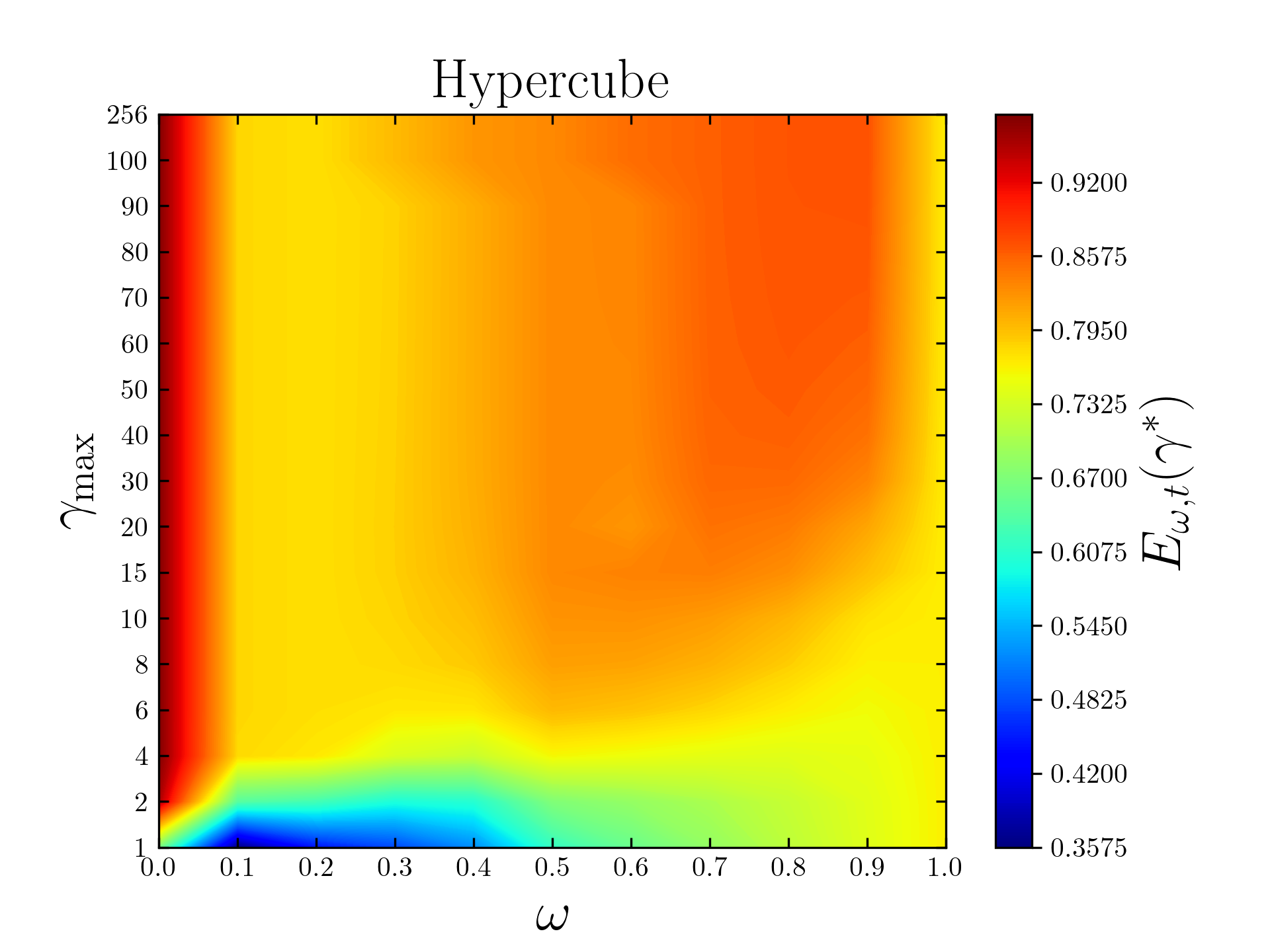
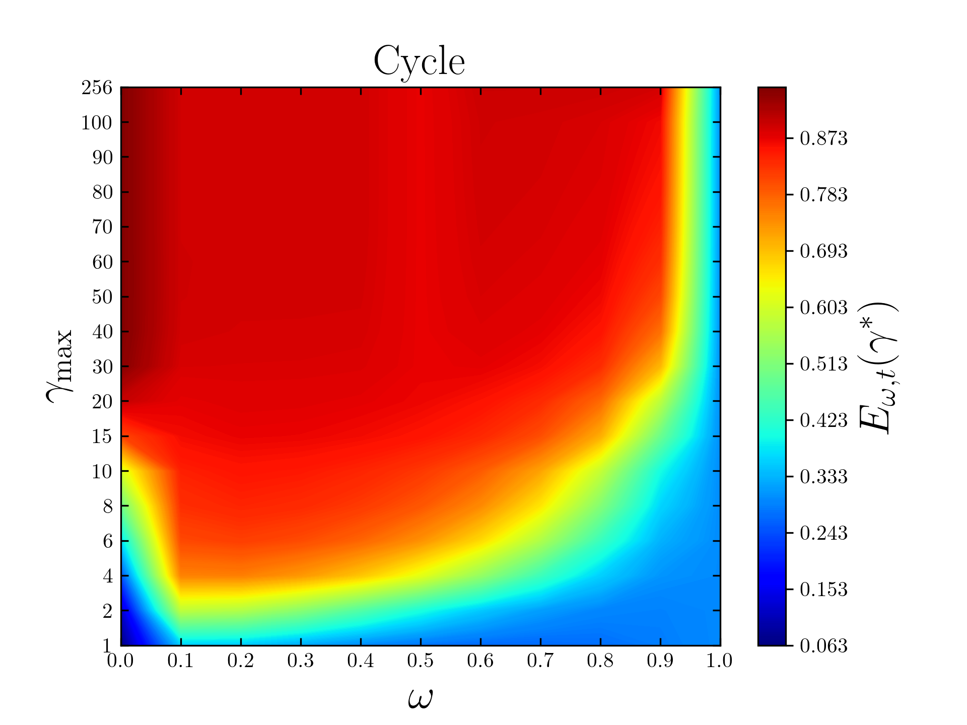
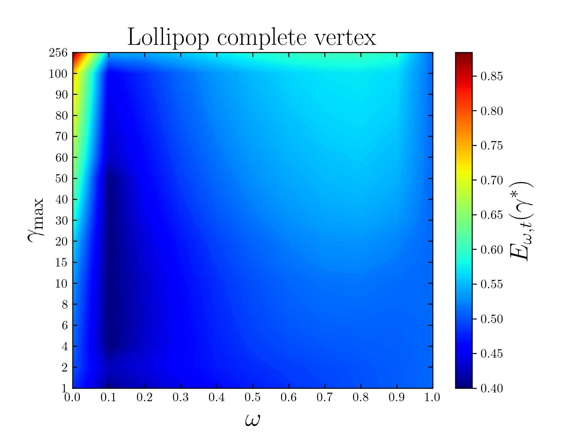
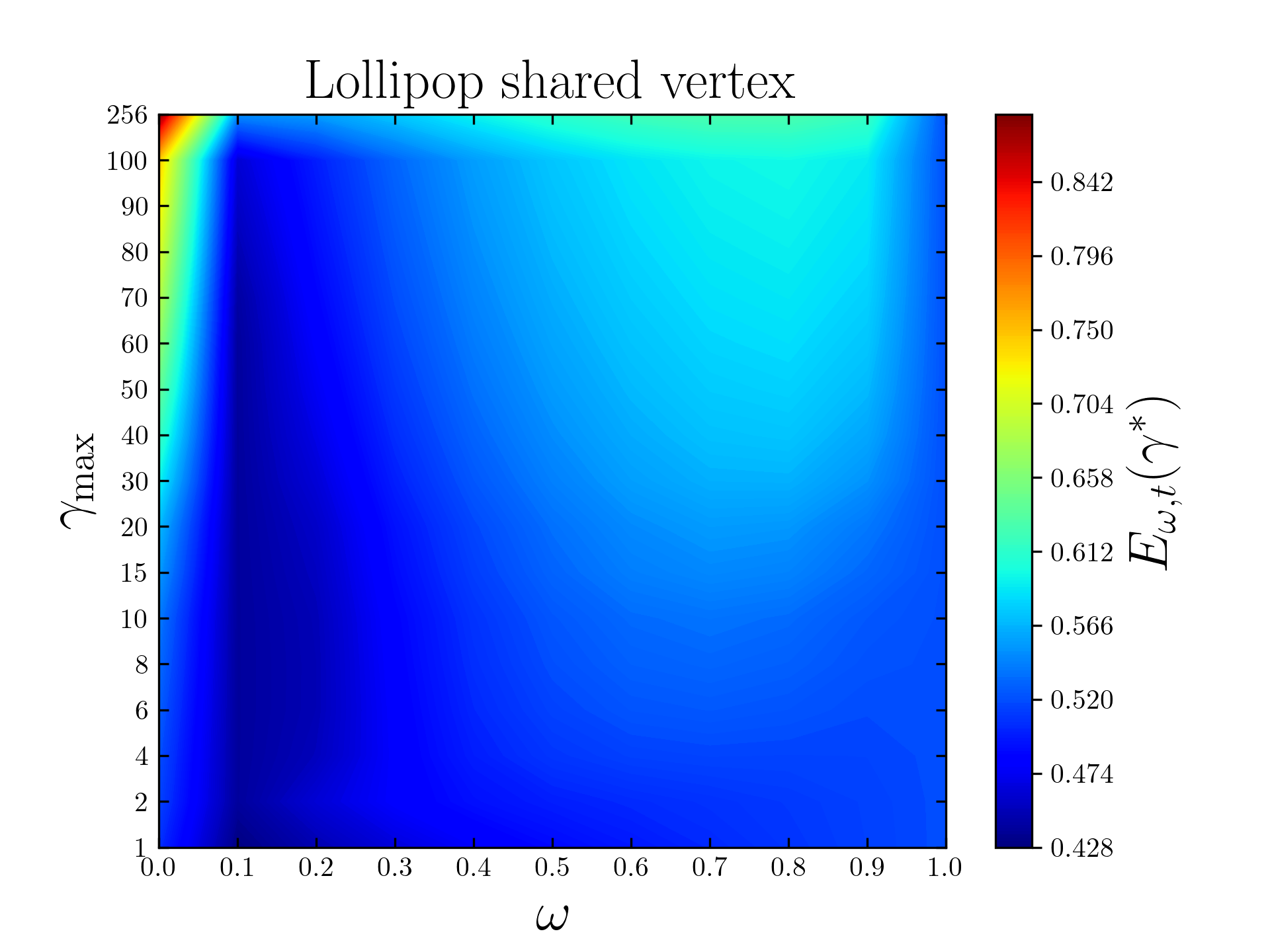
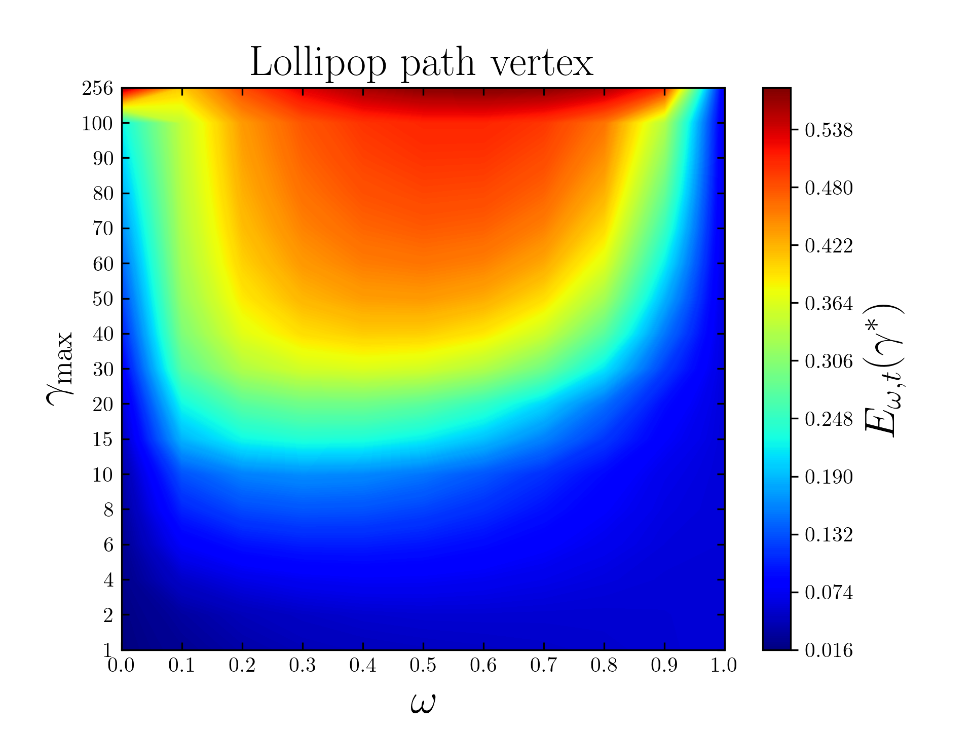
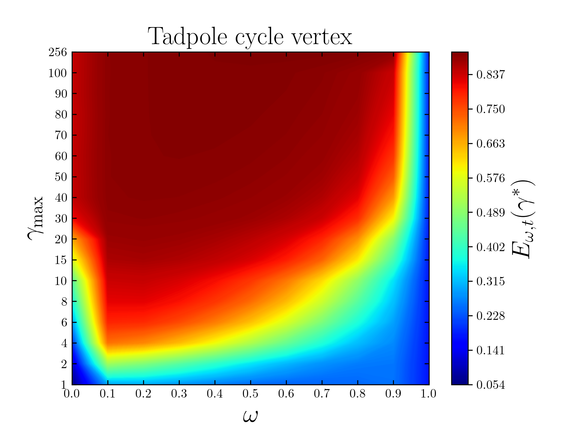
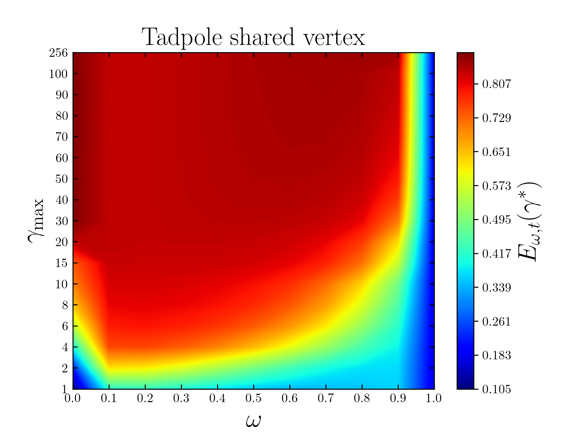
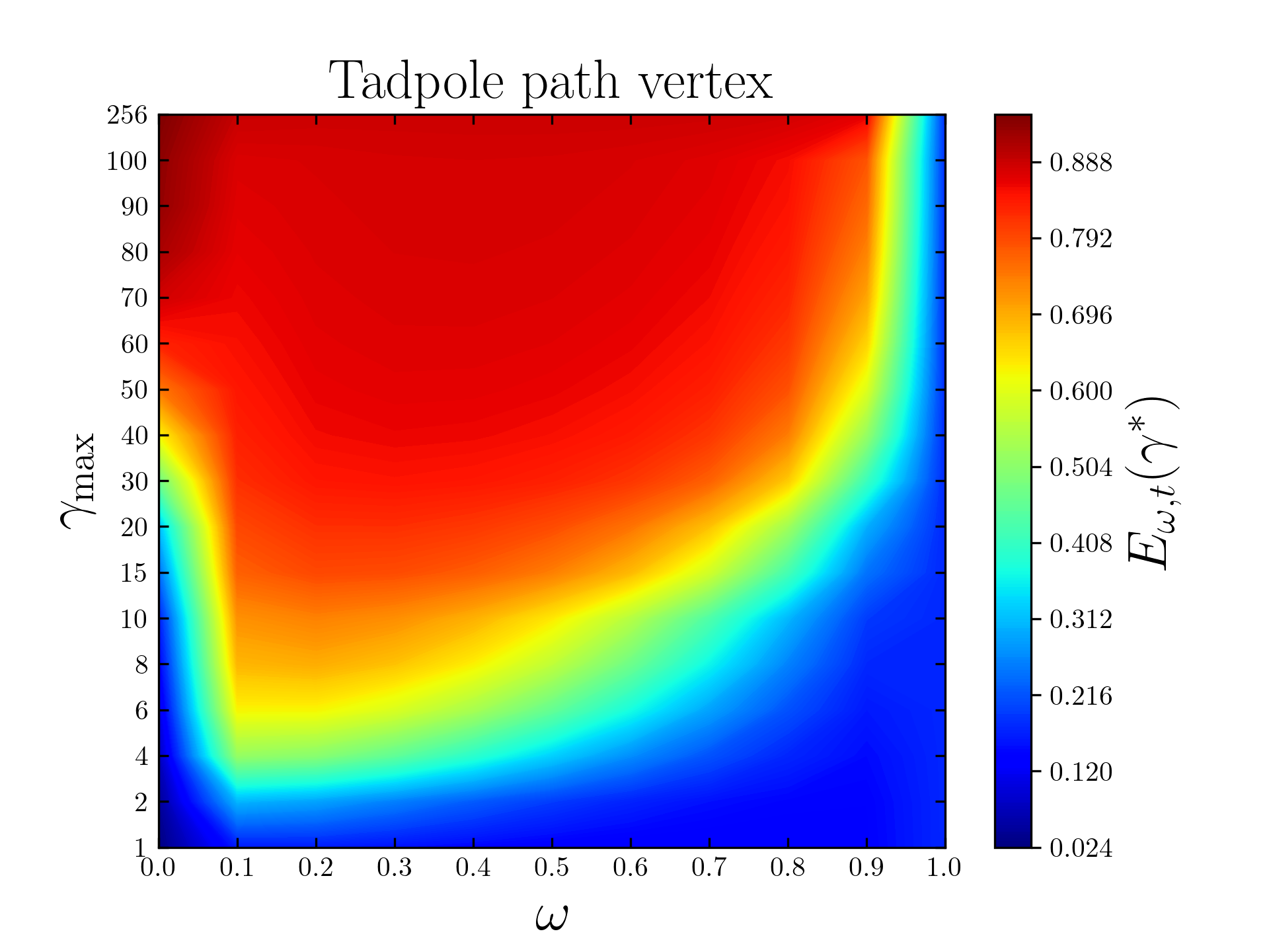
Figure 2: Stochastic Quantum Walk Search (SQWS) performances with restrained value of $\gamma_{\max}\in[1,4N]$ on the complete graph ($K_{64}$), the hypercube ($Q_{6}$), the cycle graph ($C_{64}$), the lollipop graph ($L_{32,32}$) and the tadpole graph ($T_{32,32}$). The quantum walk search is recovered for $\omega=0$, the classical random walk search for $\omega=1$, and a linear combination of the two when $\omega\in]0,1[$.

Unsurprisingly, the purely quantum regime, i.e. $\omega=0$, is the most efficient for the complete graph and the hypercube. However, for both, a hybrid regime containing little noise is less efficient than a noisier hybrid regime, and this feature is more important for the complete graph. We also note that an increase in $\gamma_{\max}$ has no impact on the complete graph, and only a variation in the interpolation parameter $\omega$ modifies the transfer efficiency. This phenomenon is not observed for the hypercube, as we can see that an increase in $\gamma_{\max}$ improves performance even if we increase the value of $\omega$, which is tantamount to increasing the importance of incoherent dynamics. The cycle graph gives completely different results: firstly, we observe that when $\gamma_{\max}<20$, certain values of $\omega$ give a more efficient hybrid regime than the quantum regime. For example, there is a difference of over 40% in transfer efficiency between the quantum and the hybrid regime for $\omega\in[0.1,0.4]$ when $\gamma_{\max}=6$. Once $\gamma_{\max}\geq 20$, the purely quantum regime becomes the most efficient, but the hybrid regime, though slightly less efficient, remains equally effective. As the value of $\gamma_{\max}$ reaches 256, we observe an average difference of 6% between the quantum and hybrid regimes, and 65% between the quantum and classical regimes. Thus, we can see that for the cycle graph mainly, and the hypercube as well, an increase in the maximum value attainable by $\gamma$ offsets the increase in $\omega$.

For the lollipop graph, we have run the SQWS on three different vertices that we call complete, shared and path. The complete vertex is an arbitrary vertex of the complete graph and shared is the vertex shared by the complete and path graphs. We also point out that the performance of the SQWS on the path graph is similar to that obtained with the cycle and we present these results in detail in Appendix B. The search results obtained for these two vertices are practically similar, and very different from those for the complete graph seen above. In fact, the introduction of a path graph into the complete graph completely alters performance. Transfer efficiency remains stuck between 40% and 60% for almost all values of $\gamma_{\max}$ and $\omega$. Only the quantum regime achieves an efficiency of over 80%, but only from $\gamma_{\max}=100$. By way of comparison, the usual complete graph reaches an efficiency of 96% from $\gamma_{\max}=1$. The path vertex is located at the extreme end of the path graph, and its search gives different results. Whatever the value of $\gamma_{\max}$, transfer efficiency to the sink does not exceed 55%. Moreover, the hybrid regime is more efficient than the quantum one when $\gamma_{\max}\leq 100$, with a difference of around 30% in efficiency when $\gamma_{\max}\in[40,70]$ between the quantum case and the hybrid for $\omega\in[0.3,0.6]$. This difference diminishes progressively with increasing $\gamma_{\max}$ and disappears almost completely to reach an average of 2% for $\omega\in[0.1,0.9]$ and 5% with the purely classical regime. The greatest difference is 16% and is observed between the quantum $\omega=0$ and the hybrid $\omega=0.1$. Although, for path a variation in the value of $\gamma_{\max}$ leads to an improvement in performance, this is still very poor compared with the search for complete and shared vertices located on the complete graph.

Finally, we ran the SQWS on the tadpole graph on the vertices cycle, shared and path. The vertex cycle is located on the cycle in such a way as to maximize the distance to shared. Unlike the previous case of the lollipop, which was made up of two graphs with very different reactions to the increase in the $\gamma_{\max}$ parameter, the tadpole graph is a fusion of two graphs with the same reaction to it. The SQWS behaves approximatively the same way for all three vertices, although we note that among the three, maximum transfer efficiency is achieved for the path search. Whereas for lollipop, the path search did not exceed 55% transfer efficiency, although a search of the complete graph was very efficient for very low values of $\gamma_{\max}$. By replacing the complete graph with a cycle, the SQWS seems to perform well again. As with the cycle, the hybrid regime requires a lower value of $\gamma_{\max}$ than the quantum regime to reach the 80% efficiency. Once again, there is a real difference in performance: for example, when $\gamma_{\max}=2$ the quantum regime has an efficiency of 7% versus around 48% for $\omega\in[0.1,0.3]$, or 16% versus around 70% on average for $\omega\in[0.1,0.5]$ when $\gamma_{\max}=10$. These significant differences in performance between the purely quantum and hybrid regimes can be observed for all three vertices. However, we note that shared requires the lowest value of $\gamma_{\max}$ to exceed the performance of the hybrid regime, followed by cycle and path.

In this study, we recover the results of Caruso et al. [53, 54] as the value $\omega=0.1$ is critical for graphs where the hybrid regime outperforms the quantum one. In these cases, we observe that the mixing $\omega=0.1$ is the first hybrid regime to outperform quantum dynamics. Moreover, we generalize their result by adding a new parameter $\gamma$ and showing that the topology of the graph plays a major role in the performance of the SQWS. The parameter $\gamma$ plays a fundamental role as it offers a balancing between the strength of the coherent exploration and the marking of the target vertex. However, we see that an increase of $\gamma$ reveals a new spectrum of the hybrid behavior as the increase of $\omega$ can be compensated with an increase of $\gamma$. Generally speaking, the SQWS behaves in a number of interesting ways, depending on the graph topology and the target vertex connectivity.The first behavior is the possibility for a hybrid regime to outperform quantum and classical dynamics for this modified search problem. On all the graphs tested, the quantum regime ends up beating the hybrid regime when $\gamma_{\max}$ reaches a high enough value. We also note that in some cases, a low-noise hybrid regime (low value of $\omega$) is less efficient than a noisier hybrid regime. This phenomenon is clearly observed for the complete graph, and also on the hypercube. Finally, we see that increasing the value of $\gamma_{\max}$ compensates for the increase in the interpolation parameter $\omega$. In other words, increasing the importance of graph exploration for the walker, and thus neglecting the oracle that enables the search, offsets the increase in the importance of incoherent operations in the system.

Intuitively, we can use metrics in an attempt to understand why the SQWS behaves differently on different graphs, and even on different vertices belonging to the same graph. A useful global graph metric is its density, with the densest complete graph serving as a reference with a density of 1. Then, two interesting local metrics for the target vertex are its eccentricity, i.e. the longest of the shortest paths to reach that vertex from any vertex in the graph, and its degree centrality, which indicates how connected the vertex is in the graph. A centrality of 1 means that the vertex is connected to all the others, and 0 to none. Interestingly, density and eccentricity are equal quantities for vertex transitive graphs, i.e. graphs whose structure does not allow vertices to be distinguished from each other. We show all these characteristics for all the graphs on which we have run the SQWS on Table 1. We can see that all the graphs where the hybrid out regime performs the quantum regime for certain values of $\gamma_{\max}$ have a high eccentricity, i.e. which scales in $\mathcal{O}(N)$. Among these graphs (cycle, path, maze, lollipop, tadpole) we also observe that the higher the eccentricity and the lower the centrality of the target vertex, then the purely quantum regime requires a higher value of $\gamma_{\max}$ to outperform the hybrid. Furthermore, we see that the lower the eccentricity and centrality, the lower the value of $\gamma_{\max}$ required for the quantum regime to perform. Finally, it seems that the higher the density and centrality, the less an increase in $\gamma_{\max}$ can compensate for the introduction of incoherent dynamics into the search.

Table 1: Global (density) and local metrics (degree centrality and eccentricity) of the target vertex for the different graphs on which we have run the Stochastic Quantum Walk Search (SQWS).

Graph	Size	Density	Target vertex $m$	Degree centrality	Eccentricity
Complete $K_{N}$	$N=64$	1	$\cdot$	1	$1=\mathcal{O}(1)$
Cycle $C_{N}$	$N=64$	0.0317	$\cdot$	0.0317	$32=\lfloor N/2\rfloor=\mathcal{O}(N)$
$d$-Hypercube $Q_{d}$	$N=2^{d}=64$	0.0952	$\cdot$	0.0952	$6=d=\mathcal{O}(\log N)$
	($d=6$)
Grid $G_{\sqrt{N}\times\sqrt{N}}$	$N=81$	0.0444	center	0.05	$8=\sqrt{N}-1=\mathcal{O}(\sqrt{N})$
			border	0.025	$16=2(\sqrt{N}-1)=\mathcal{O}(\sqrt{N})$
Star $S_{N-1}$	$N=64$	0.0312	center	1	$1=\mathcal{O}(1)$
			border	0.0158	$2=\mathcal{O}(1)$
Wheel $W_{N}$	$N=64$	0.0625	center	1	$1=\mathcal{O}(1)$
			border	0.0476	$2=\mathcal{O}(1)$
Perfect Binary Tree	$N\!=\!2^{d+1}\!-\!1\!=\!63$	0.0317	$d_{m}=0$ (root)	0.0322	$5=d+d_{m}=\mathcal{O}(\log N)$
			$d_{m}=3$	0.0483	$8=d+d_{m}=\mathcal{O}(\log N)$
$PBT_{d}$ of depth $d$	($d=5$)		$d_{m}=5$ (leaf)	0.0161	$10=d+d_{m}=\mathcal{O}(\log N)$
Path $P_{N}$	$N=65$	0.0307	center	0.0312	$32=\lfloor N/2\rfloor=\mathcal{O}(N)$
			border	0.0156	$64=N-1=\mathcal{O}(N)$
Lollipop $L_{M,N}$	$M$+$N\!=\!32$+$32$	0.2619	complete	0.4920	$33=N+1=\mathcal{O}(N)$
			shared	0.5079	$32=N=\mathcal{O}(N)$
			path	0.0158	$33=N+1=\mathcal{O}(N)$
Tadpole $T_{M,N}$	$M$+$N\!=\!32$+$32$	0.0317	cycle	0.0317	$48\!=\!N+\lfloor M/2\rfloor=\mathcal{O}(N$+$M)$
			shared	0.0476	$32\!=\!\max(N,\lfloor M/2\rfloor)\!=\!\mathcal{O}(N$+$M)$​
			path	0.0158	$48\!=\!N+\lfloor M/2\rfloor\!=\!\mathcal{O}(N$+$M)$
Random (Small-World)	$N=66$	0.0867	HC	0.1846	6
			IC	0.0923	6
$SW_{N}$			LC	0.0615	5
Maze $M_{N}$	$N=73$	0.0138	exit	0.0273	34

We explore the behavior of the SQWS on many different families of graphs, and observe how it behaves when a cycle is gradually transformed into a complete graph in Appendix B.

III.2 Relation to entropy

We now relate the optimal interpolation regime $\omega$ to the evolution of the Von Neumann entropy of the system:

$$S(\rho)=-\text{Tr}\left({\rho\ln\rho}\right).$$ (11)

We observe for every run of the SQWS that the entropy first increases up to a maximum, and then decreases until it converges to zero. We also observe that when an increase in the maximum value of $\gamma$ increases the performance of the SQWS, i.e. the transfer to the sink, this translates into a reduction in the time needed to reach the entropy maximum and a faster convergence to zero thereafter. Furthermore, we observe that the optimal interpolation regime $\omega$ is that whose entropy converges to zero the fastest. The presence of the sink vertex $\phi$ introduces dissipation in the system, therefore, as $t\rightarrow\infty$ the walker will end up in the sink with a probability of 1. Thus, the state of the walker converges from $\rho(0)$ to the projector $\ket{\phi}\bra{\phi}$. Although zero entropy indicates a pure state, it does not guarantee that this state is the state towards which the system converges. Therefore, we also compute the $l_{1}$-norm coherence, which is the sum of the off-diagonal elements of $\rho$:

$$C_{l_{1}}(\rho)=\sum_{i\neq j}|\rho_{ij}|.$$ (12)

As the initial state is the uniform superposition over the set of vertices $V$, the initial value is $C_{l_{1}}(\rho(0))=|V|-1$. For all graphs on which we run the SQWS, we observe that this quantity decreases monotonically and it converges to zero. Thus, the convergence of entropy to zero does indicate that the walker state is getting closer and closer to the state $\ket{\phi}\bra{\phi}$, as $\rho$ becomes increasingly diagonal over time. We illustrate the entropy evolution over time in Fig. 4 for the complete graph, the hypercube, the cycle graph and the lollipop graph (for the path vertex). Looking at Fig. 4(a), we note that whatever the value of $\gamma_{\max}$, the evolution of entropy does not change for the complete graph. On the other hand, the evolution of entropy for the other graphs with the value of $\gamma_{\max}$, and this phenomenon is particularly visible for the purely quantum regime, i.e. $\omega=0$). In particular, we see a big change for the hypercube when $\gamma_{\max}$ goes from 1 to 2 in Fig. 4(b). We see, for example, that when $\gamma_{\max}=60$, the most efficient regime is quantum, and among the noisy regimes, the most efficient is $\omega=0.8$ in Fig. 2. We can also see this phenomenon in Fig. 4(b) as the fastest convergence to zero after $\omega=0$ is indeed for $\omega=0.8$. However, when $\gamma_{\max}=100$, we see that $\omega=0.9$ becomes the noisy regime with the fastest convergence, which is also verified in Fig. 2. As for the cycle graph, we see in Fig. 4(c) that as we increase $\gamma_{\max}$, the time $t_{S}$ needed to reach the maximum entropy value for the different $\omega$ values decreases, and convergence to 0 is faster too. For the cycle graph, the purely quantum regime becomes more efficient than the hybrid from $\gamma_{\max}=20$. This behavior can be clearly seen from the fact that, from this value onwards, the entropy that converges to 0 most rapidly is that of the purely quantum regime, i.e. $\omega=0$. The case of lollipop is interesting because, as we can see in Fig. 2, the performance does not exceed 30% efficiency until after reaching $\gamma_{\max}=30$ for the hybrid regime. This sudden change in performance can be seen in Fig. 4(d) as we see that entropy decay towards 0 is faster when $\gamma_{\max}\geq 30$. Moreover, we see that the time $t_{S}$ decreases more and more with increasing parameter $\gamma_{\max}$ for the hybrid regime. For the purely quantum case, we observe a change in efficiency from $\gamma_{\max}=100$, which translates into a shorter time $t_{S}$, as well as a better convergence to 0 of the entropy. However, convergence remains weak for all interpolation values $\omega$, as the maximum efficiency does not exceed 55%. In general, we can clearly see from Fig. 4 that the efficiency of transfer to the sink translates firstly into a reduction in the time $t_{S}$ needed to reach maximum entropy. Then, by a convergence of entropy towards zero as quickly as possible, where the $\omega$-regime maximizing efficiency is the one with the fastest convergence.

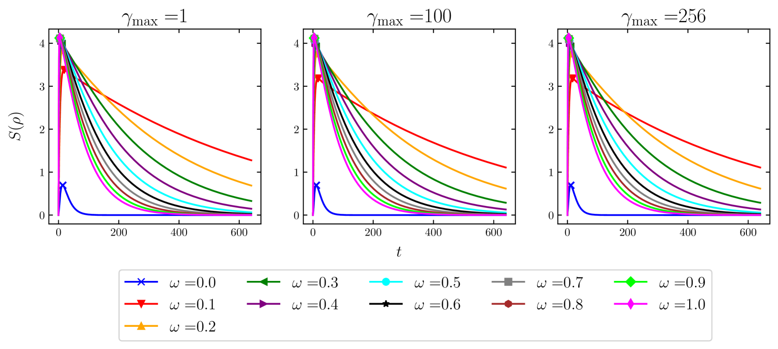
(a) Complete graph

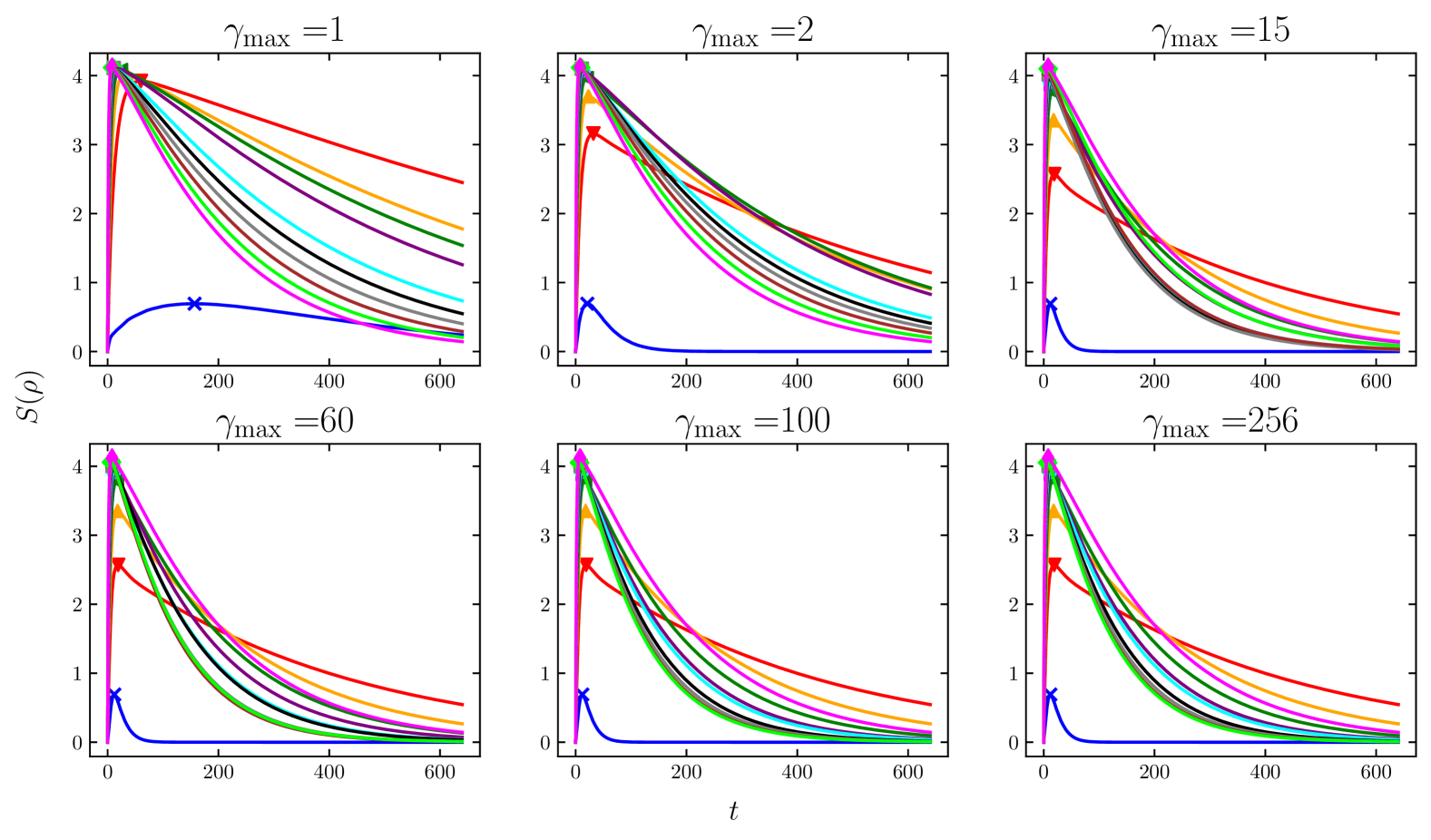
(b) Hypercube

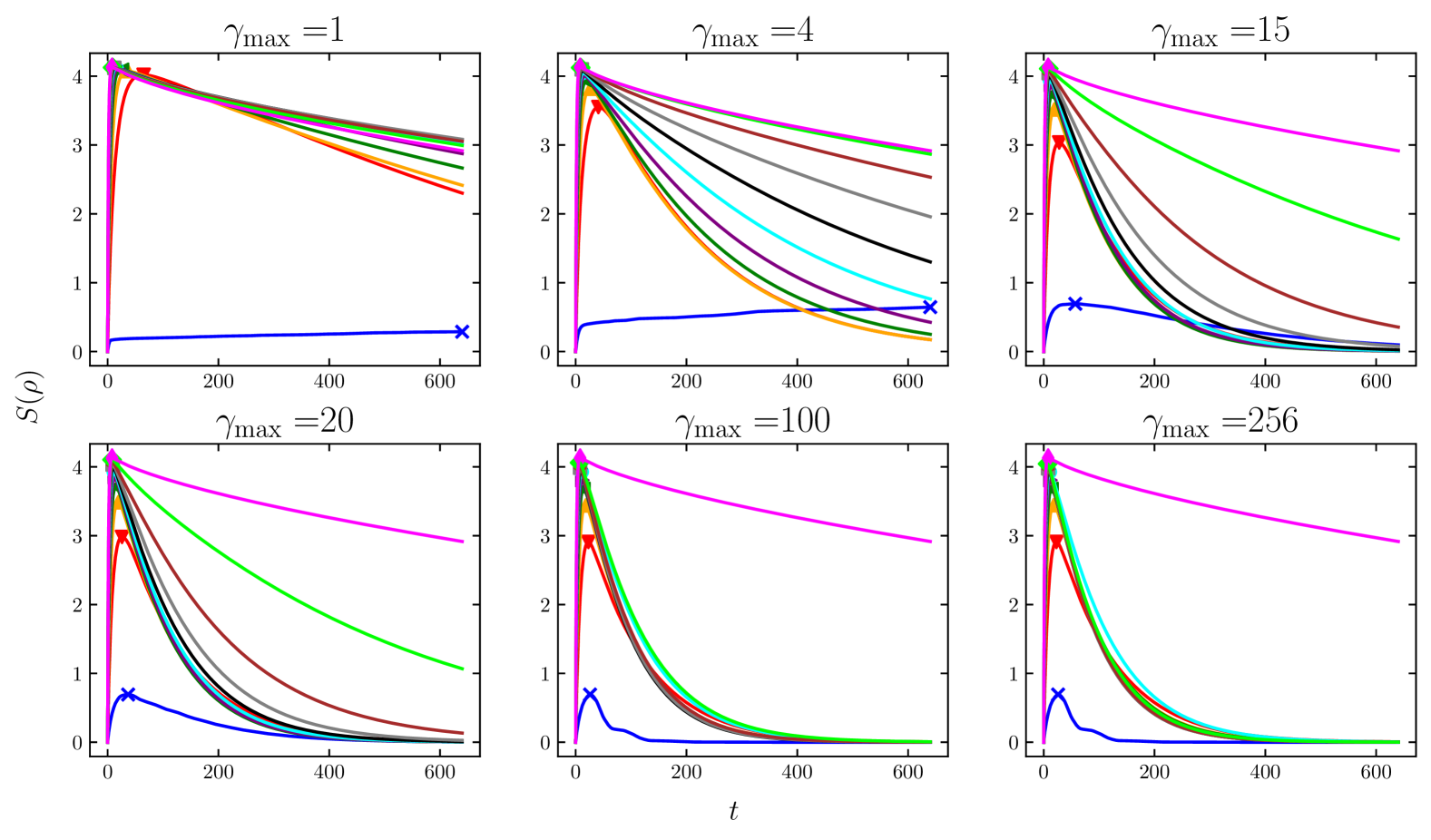
(c) Cycle graph

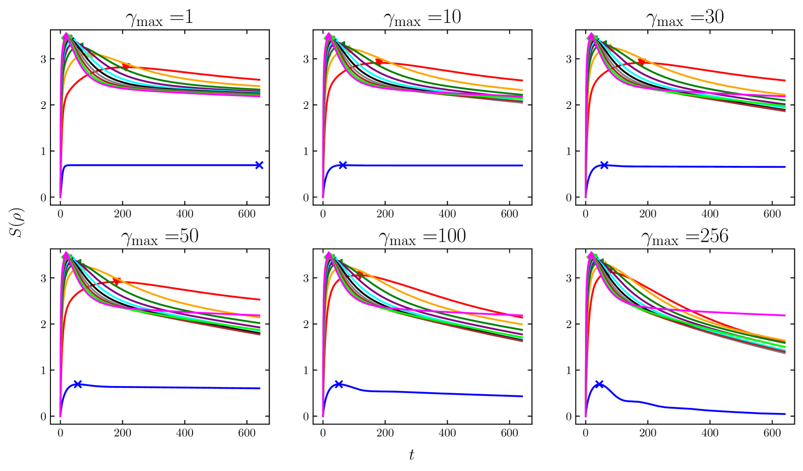
(d) Lollipop graph path vertex

Figure 4: Von Neumann entropy $S(\rho)$ as a function of time $t$ for different values of $\gamma_{\text{max}}$ for the complete graph $K_{64}$, the 6-hypercube $Q_{6}$, the cycle graph $C_{64}$ and the lollipop graph $L_{32,32}$ for the path vertex. The markers indicate the time $t_{S}$ at which the entropy reaches its maximum value before decreasing down to zero.

We also illustrate the reduction of duration $t_{S}$ required to reach the maximum entropy in Fig. 5 for these graphs. For the complete graph, we observe a slight reduction in this time for $\omega\in\{0,0.1\}$ as $\gamma_{\max}$ increases from 1 to 2. Otherwise, the duration $t_{S}$ remains totally unaffected by an increase in $\gamma_{\max}$. We point out that the evolution of $t_{S}$ is constant for the classical case for all graphs, i.e. $\omega=1$, as the parameter $\gamma$ lies in the Hamiltonian. We observe that for the hypercube, this duration decreases significantly with increasing $\gamma_{\max}$. Interestingly, we note that for $\omega\in[0.2,0.4]$, this duration increases slightly, then decreases again for $\omega=0.4$ and remains constant for the others. This means that the value of $\gamma_{\max}$ which maximizes the efficiency of the SQWS for a given value of $\omega$, is not necessarily the one which minimizes the duration $t_{S}$. For these values of $\omega$, the increase does not exceed 7 units of time (for a total evolution of 640 times units). For the cycle and the lollipop graphs, we observe a monotonic decay of $t_{S}$ as $\gamma_{\max}$ increases, and we note that the decay for the quantum regime of the lollipop begins only from $\gamma_{\max}=100$ and then a little more significantly at $\gamma_{\max}=256$, since it is from these values that the efficiency begins to increase. Therefore, given a value of $\gamma$, we observe that the optimal interpolation regime $\omega$ in our framework is the one that leads to the fastest convergence to zero entropy. Furthermore, an increase in the value of $\gamma$ can improve the SQWS performance if it results in a significant reduction in the time needed to reach maximum entropy.

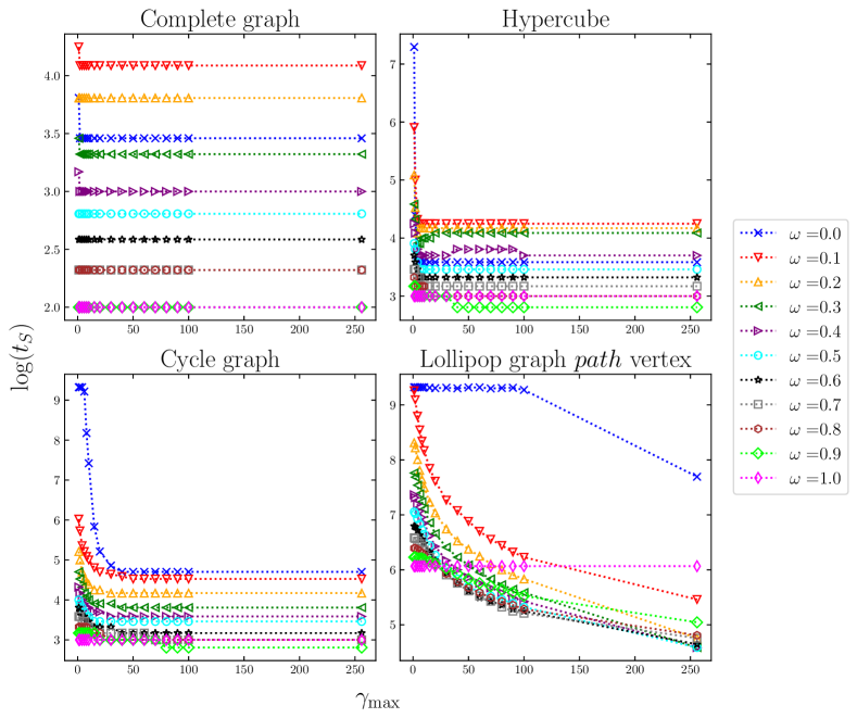
Figure 5: Evolution of the duration $t_{S}$ needed to reach maximum entropy as a function of $\gamma_{\text{max}}$ for the complete graph $K_{64}$, the 6-hypercube $Q_{6}$, the cycle graph $C_{64}$ and the lollipop graph $L_{32,32}$ (with path vertex) for different values of interpolation $\omega\in[0,1]$.

IV Conclusion

In summary, we have studied a continuous-time search problem in which the walker explores a graph according to a searching dynamics driven to a specific target vertex. We also connected a trapping sink vertex to the target with an irreversible transition. We extended the result of Caruso et al. [53, 54] to a Stochastic Quantum Walk Search (SQWS) and we numerically showed that a tunable mixing of unitary and non-unitary dynamics can outperform a non-hybrid evolution for this problem depending on (i) the graph topology, (ii) the target vertex connectivity and (iii) a parametrized Hamiltonian. In particular, the Hamiltonian parameter controls the balance between the coherent exploration and the importance of the oracle used to mark the target vertex. We have also related the optimal tunable mixing of unitary and non-unitary operations to the system entropy decay rate. Moreover, we have shown that the hybrid regime can beat the purely quantum dynamics only in the presence of a trapping sink. For numerous graphs, mostly sparse, quantum evolution requires to increase the Hamiltonian parameter to achieve the same performance. Therefore, by considering the value of this parameter as a computational resource, the hybrid evolution may require fewer resources than the quantum to perform. More importantly, at a fixed parameters configuration, we can still play with the interaction graph to fit the optimal transfer performance. This can pave the way to a technological leap where noise can be seen as a useful physical resource, in a hardware setting where one can change the connectivity of the architecture for reliable quantum computing. In conclusion, future work could also focus to provide a natively circuit based model for the above results, introducing quantum noise as close as possible to real physical devices’.

V Data availability

Simulations were carried out with the Python library QuTip [63] and the graphs were generated with NetworkX [64]. The code is available at: SQWS.

VI Acknowledgements

We thank Ravi Kunjwal, Joachim Tomasi, Julien Zylberman and Sunheang Ty for their usefull feedback on the form and content of this manuscript. This work is supported by the PEPR EPiQ ANR-22-PETQ-0007, by the ANR JCJC DisQC ANR-22-CE47-0002-01.

Appendix A SQWS with no sink

In this section, we briefly discuss the performances of the SQWS with no use of an extra sink vertex connected to the target vertex. We set $\Gamma=0$ in Eq. (9). This setting corresponds to the usual quantum search problem when $\omega=0$ as the success probability is now related to the presence of the walker in the target vertex $m$ instead of the sink. Therefore, the cost function to maximize is the usual spatial search success probability:

$$P_{\omega,t}(\gamma)=\text{Tr}\left({\mathcal{E}[\rho(t)]\ket{m}\bra{m}}\right).$$ (13)

Childs and Goldstone search provides a quadratic speedup for the complete graph and the hypercube [42], meaning that the evolved state $\mathcal{E}[\rho(t)]$ reaches a large overlap with the target $\ket{m}\bra{m}$ in a timeframe that scales as $t=\mathcal{O}(\sqrt{|V|})$, which is not the case for the cycle graph [60]. Therefore, we run the SQWS on instances of the complete graph, the hypercube and the cycle graph and show the results in Fig. 6. Unsurprisingly, the introduction of non-unitary operations, i.e. increasing the value of $\omega$, drastically reduces search performance. For the complete graph and the hypercube, we still observe a peak reached in a time scaling quadratically with their size when $\omega\leq 0.4$. However, the maximum amplitude reached is much lower than that obtained for the purely unitary evolution, i.e. $\omega=0$. Furthermore, for the complete graph and the hypercube, once $\omega>0.4$, we observe a change in behavior. As there is no longer any oscillatory behavior and we get that $\gamma^{*}=0$, the success probability suddenly converges to 1. However, the time taken to approach 1 no longer scales quadratically with the size of the graph. As for the cycle graph, it is clear that the search does not work even for the quantum case. There is a slight oscillation as long as $\omega\leq 0.3$, then a jump in performance from $\omega=0.4$. However, when $\omega\in[0.4,1]$, although the maximum amplitude reached continues to increase, it follows a very slow growth rate, not exceeding 0.3 when those of the complete graph and the hypercube are very close to 1.

Therefore, we can see that simply removing the sink term completely changes the reaction of the SQWS to the introduction of non-unitary operations. In the presence of a sink, the transfer to the sink can be much more efficient in a noisy regime than in a purely quantum one, based on the graph topology, the target vertex connectivity, and the value of $\gamma_{\max}$. Hence, the addition of non-unitary operations is not usefull if the graph does not have an extra trapping site.

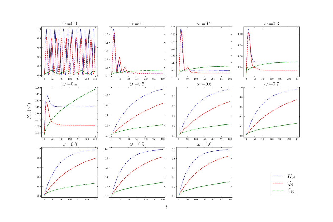
Figure 6: Success probability $P_{\omega,t}(\gamma)$ as a function of time $t$ of finding the target vertex using the Stochastic Quantum Walk Search (SQWS) with no sink vertex connected to the target vertex, i.e. $\Gamma=0$ in Eq. (9), on the complete graph ($K_{64}$), the 6-dimensional hypercube ($Q_{6}$) and the cycle graph ($C_{64}$). The usual quantum walk search is recovered for $\omega=0$, the classical random walk search for $\omega=1$, and a linear combination of the two when $\omega\in]0,1[$.

Appendix B SQWS with sink

In this section, we take the numerical study of the SQWS a step further by running it on numerous instances of different graph families.

B.1 Additional graphs

We now run the SQWS exclusively on non-vertex transitive graphs, i.e. graphs with a structure that distinguishes their vertices. We select the path graph ($P_{N}$), the star graph ($S_{N-1}$), the wheel graph ($W_{N}$), the 2D-grid ($G_{\sqrt{N}\times\sqrt{N}}$), the perfect binary tree of depth $d$ ($PBT_{d}$), a maze graph ($M_{N}$) and a random graph ($SW_{N}$) constructed by gluing together three small-world graphs of 22 vertices each with different average connectivity and rewiring probabilities [65]. We show the graph $SW_{66}$ in Fig. 8 and the results of the SQWS on these graphs in Fig. 7. For the maze we mark the exit vertex and for the path, the center and one of the two end vertices, which we call border. The behavior of the maze and path graphs is similar to that of the cycle observed in Fig. 2. The hybrid regime outperforms the quantum one up to a certain value of $\gamma_{\max}$. Moreover, we note that this critical value, where quantum outperforms hybrid, is highest when searching for a vertex located at the path extremity. We also note that this vertex has the highest eccentricity of all the vertices on which we have run the SQWS (see Table 1). For these two graphs, an increase in $\gamma_{\max}$ compensates for the increase in $\omega$, as the hybrid regime performs almost as well as the quantum one for high values of $\gamma_{\max}$. For the star and wheel graphs, unsurprisingly, we obtain very different behavior depending on the marked vertex. When the search concerns the central vertex connected to the whole network, the results are similar to those for the complete graph, i.e. the quantum regime is the most efficient from $\gamma_{\max}=1$. However, unlike the complete graph, performance decreases with increasing $\omega$. This behavior was not observed for the complete graph, where strangely enough, a low-noise regime was less efficient than a high-noise regime. We also note that the star graph is less sensitive to the introduction of noise than the wheel, as performance decreases less rapidly with increasing $\omega$. However, if we do not search for the central vertex, the behavior of the SQWS changes completely. This time, a much higher value of $\gamma_{\max}$ is required to achieve an efficiency of around 80%. Moreover, the hybrid regime is more efficient than the quantum one when $\gamma_{\max}<8$, but transfer efficiency remains under 40%. Above a certain value of $\gamma_{\max}$, 30 for the star and 15 for the wheel, the quantum regime outperforms the hybrid. We also observe that it is more difficult to stabilize hybrid performance with the increase of $\omega$ for the star than for the wheel graph. Finally, the behavior of the SQWS on the remaining graphs, i.e. the 2D-grid, the perfect binary tree and the random graph composed of three small-world graphs, are quite similar. In each case, the quantum regime becomes more efficient than the hybrid for low values of $\gamma_{\max}$. We note, however, that the grid is the graph for which the hybrid best compensates for the increase in non-unitary dynamics by the increase in $\gamma_{\max}$, especially when the marked vertex is at one of the extremities. This compensation is least present for the binary tree when searching for the vertex located at depth 5, i.e. the leaf. In this case, the hybrid regime struggles to catch up with the performance of the quantum one once it has passed it. Furthermore, it is for the search of this vertex that the quantum regime requires the highest value of $\gamma_{\max}=15$ to exceed 80% efficiency among these last three graphs. For the binary tree, the most efficient search in general for the hybrid regime is for the vertex located at depth 3 (note that 0 corresponds to the root). From $\gamma_{\max}=40$ the hybrid scheme has a uniform efficiency of around 80% for $\omega\in[0.1,0.9]$. This is not the case for the root search, where we observe one of the same phenomenon as for the complete graph, i.e. that a low-noise regime is less efficient than a noisier one. Finally, the search on the random graph gives rather equivalent results for the three vertices searched. The quantum regime exceeds 80% efficiency for very low values of $\gamma_{\max}$, then increasing this same parameter compensates for the increase in $\omega$. As in the case of the binary tree, we can see that the higher the connectivity of the vertex we are looking for, the more efficient the high-noise regime is compared to the low-noise one, although the difference is very small compared to what we observed for the complete graph.

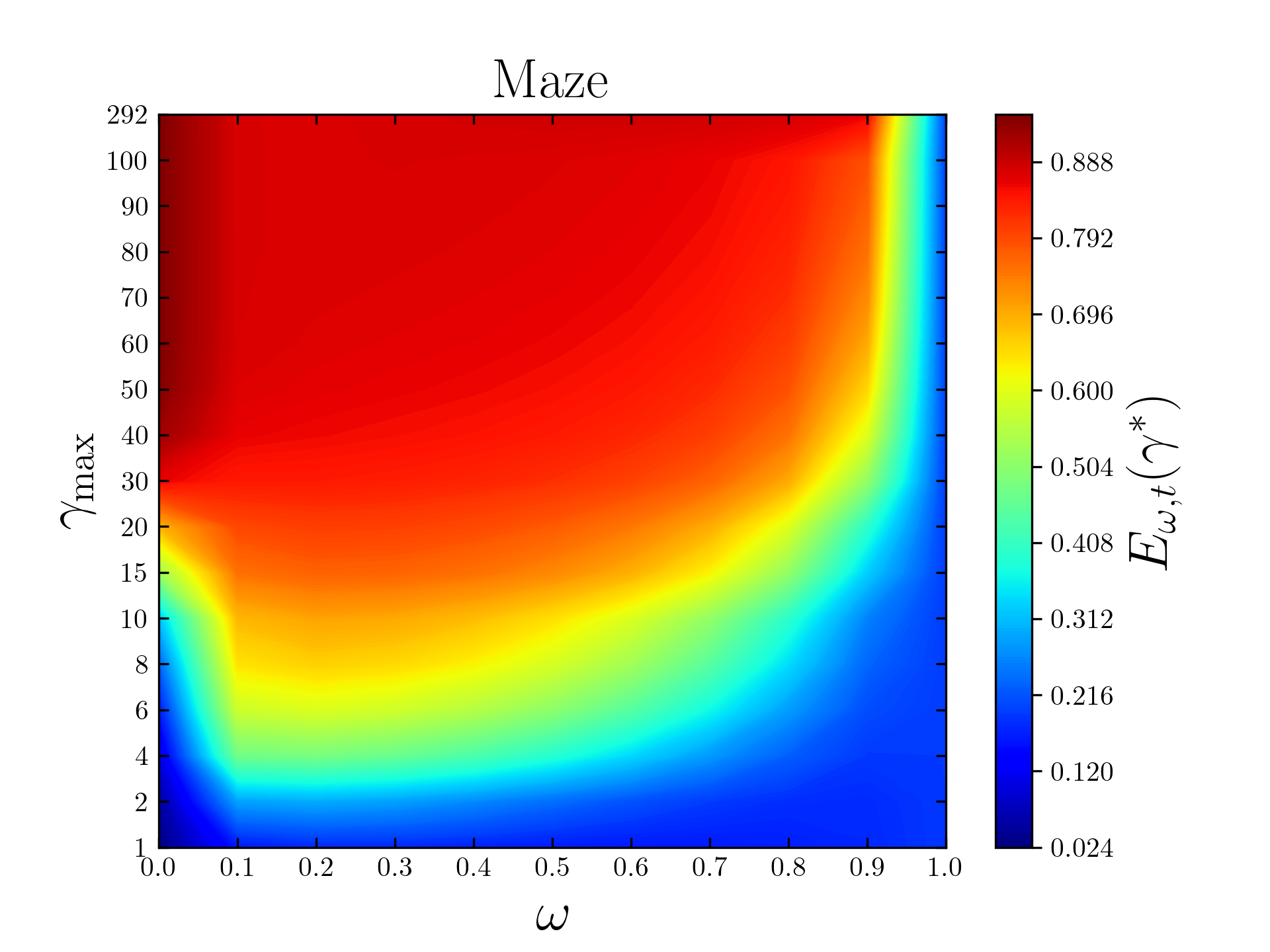
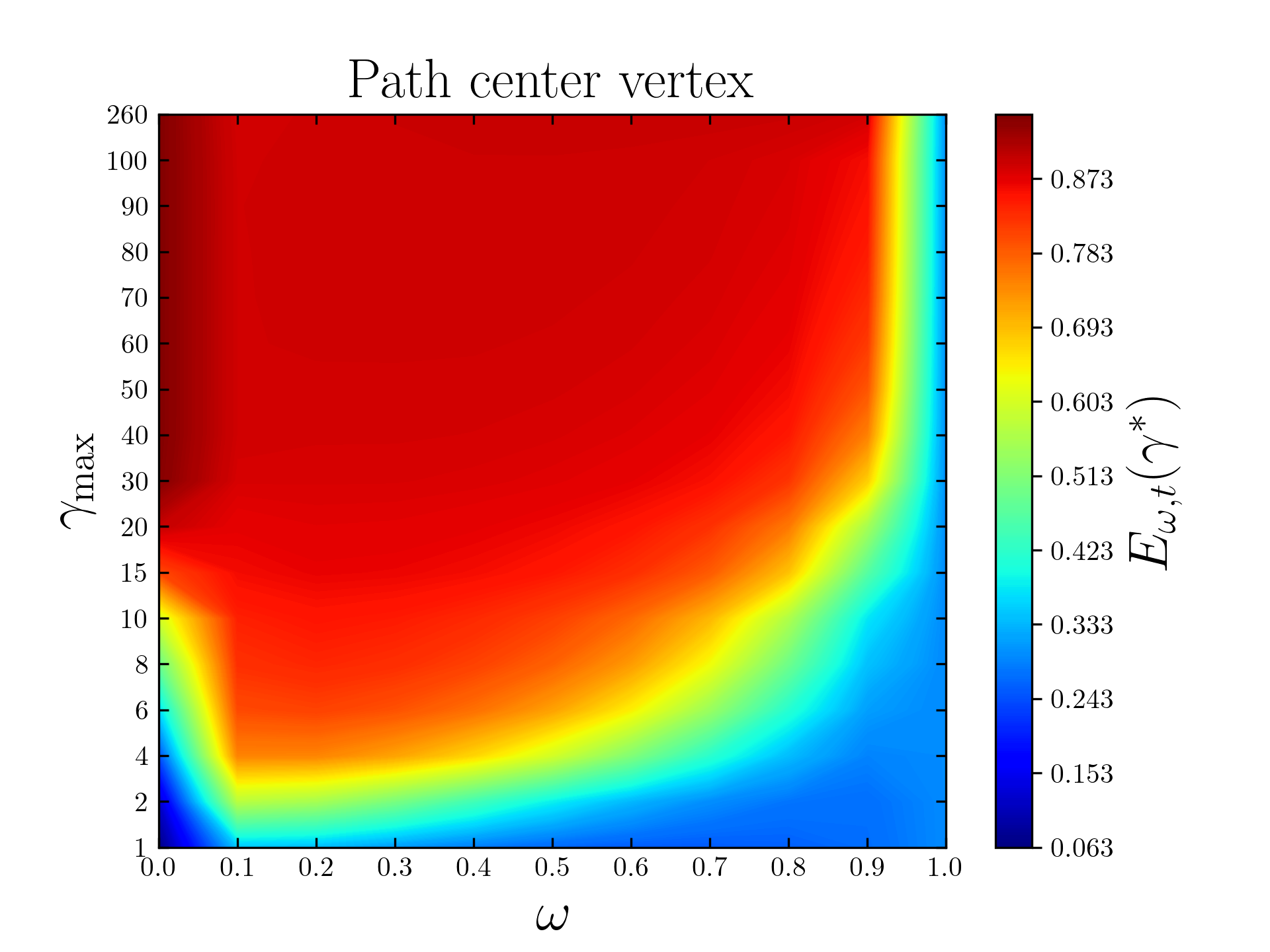
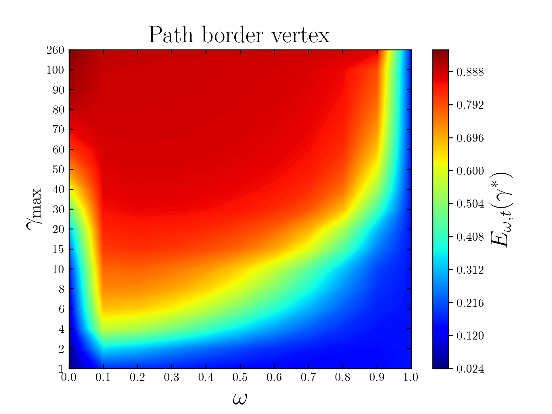
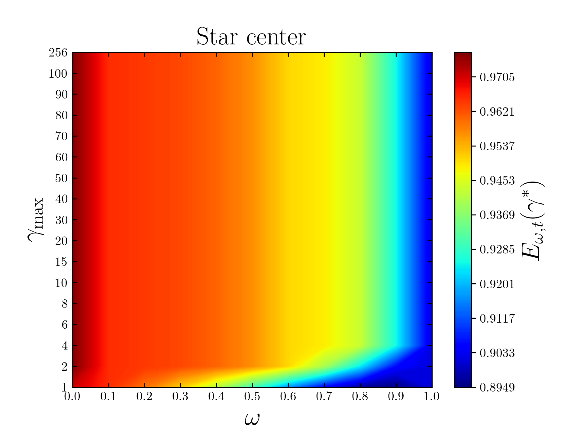
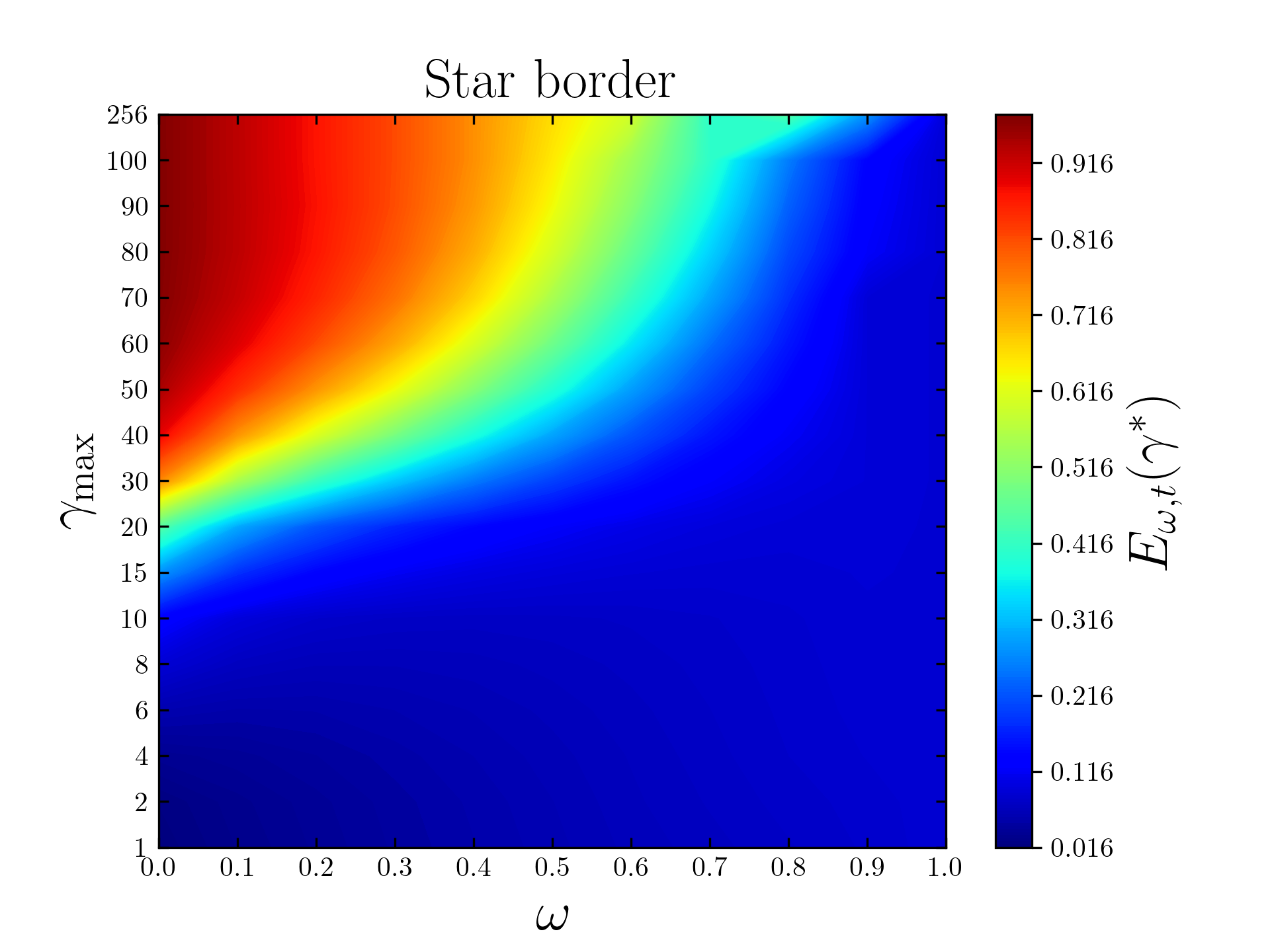
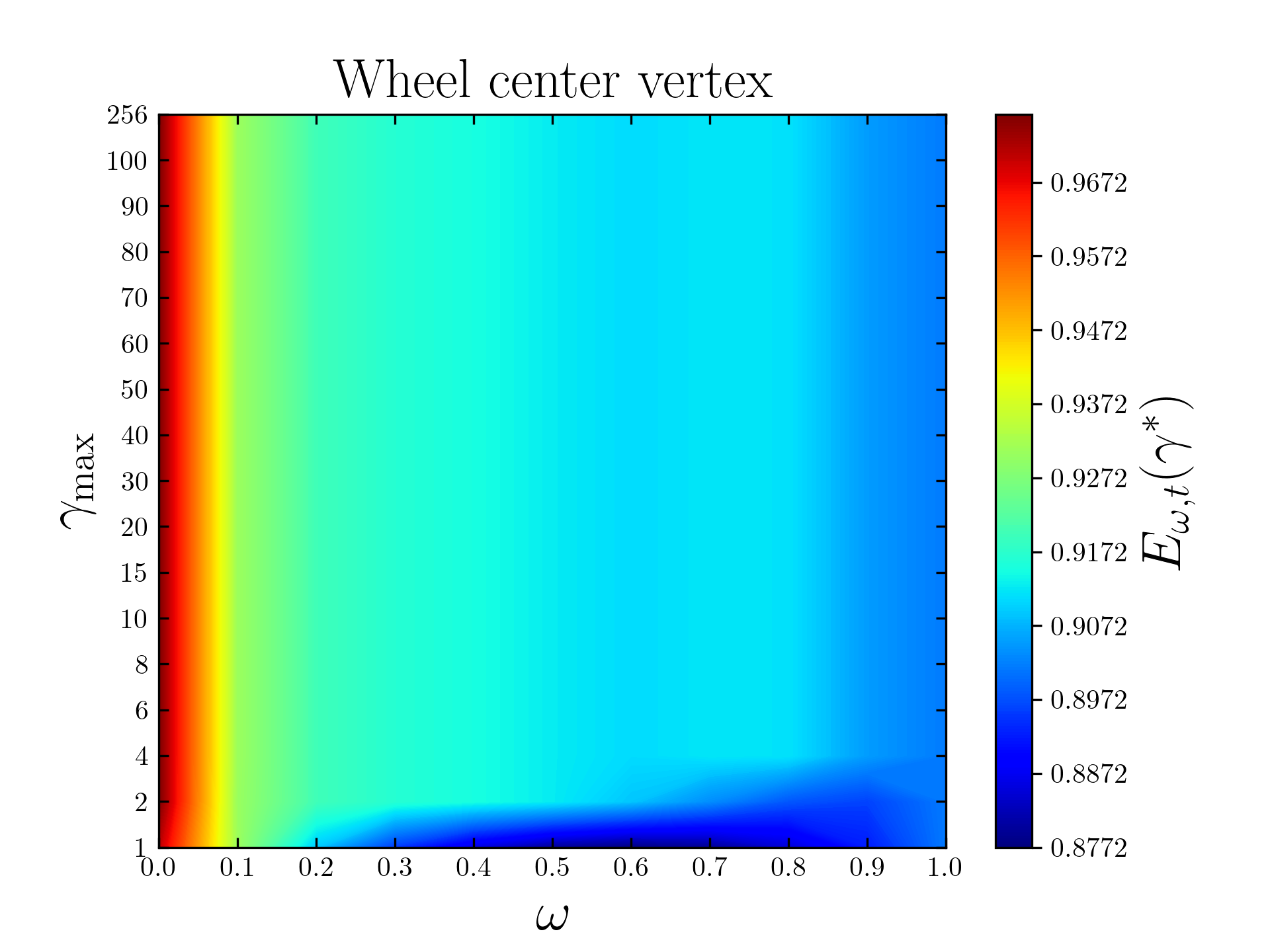
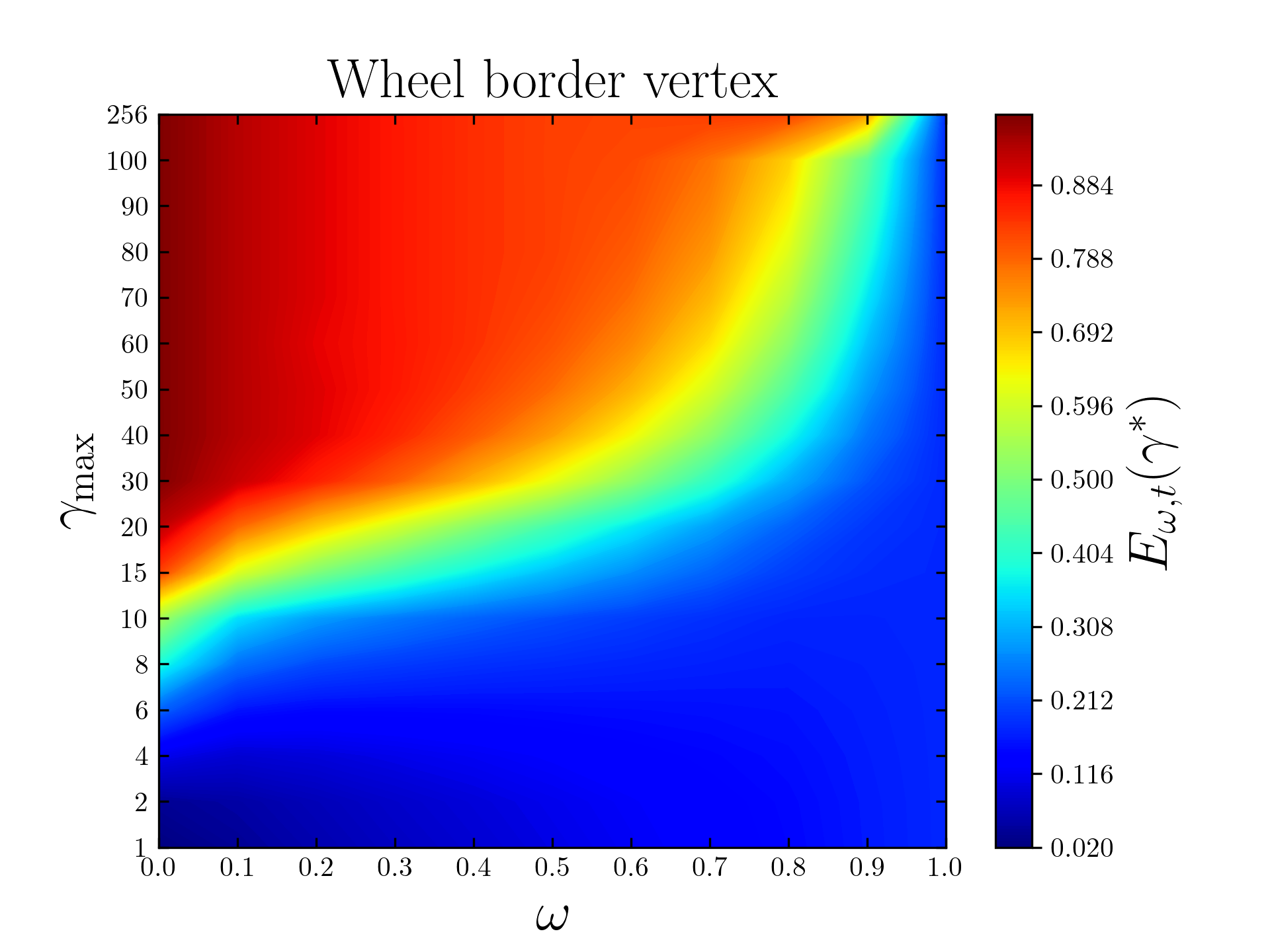
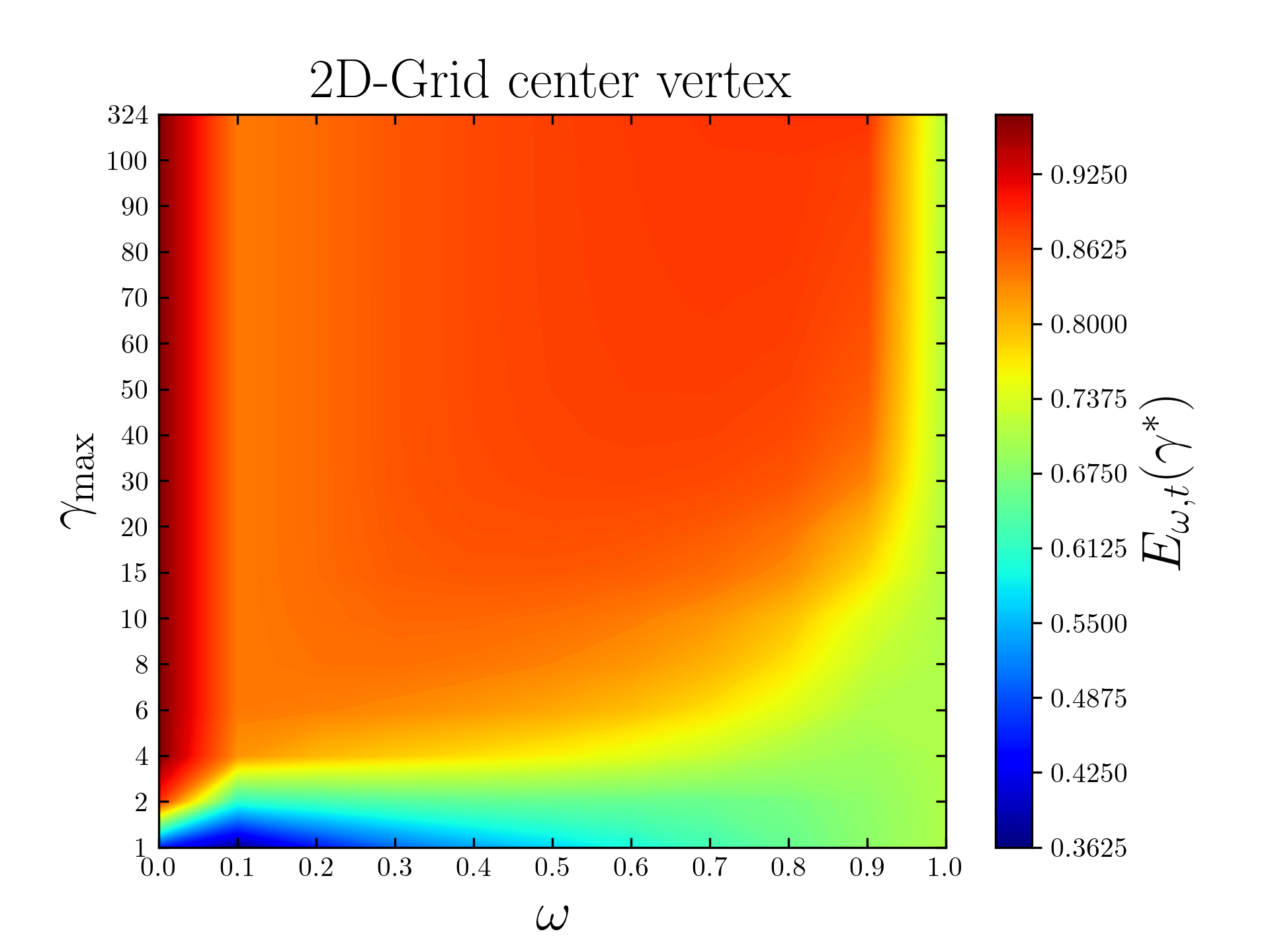
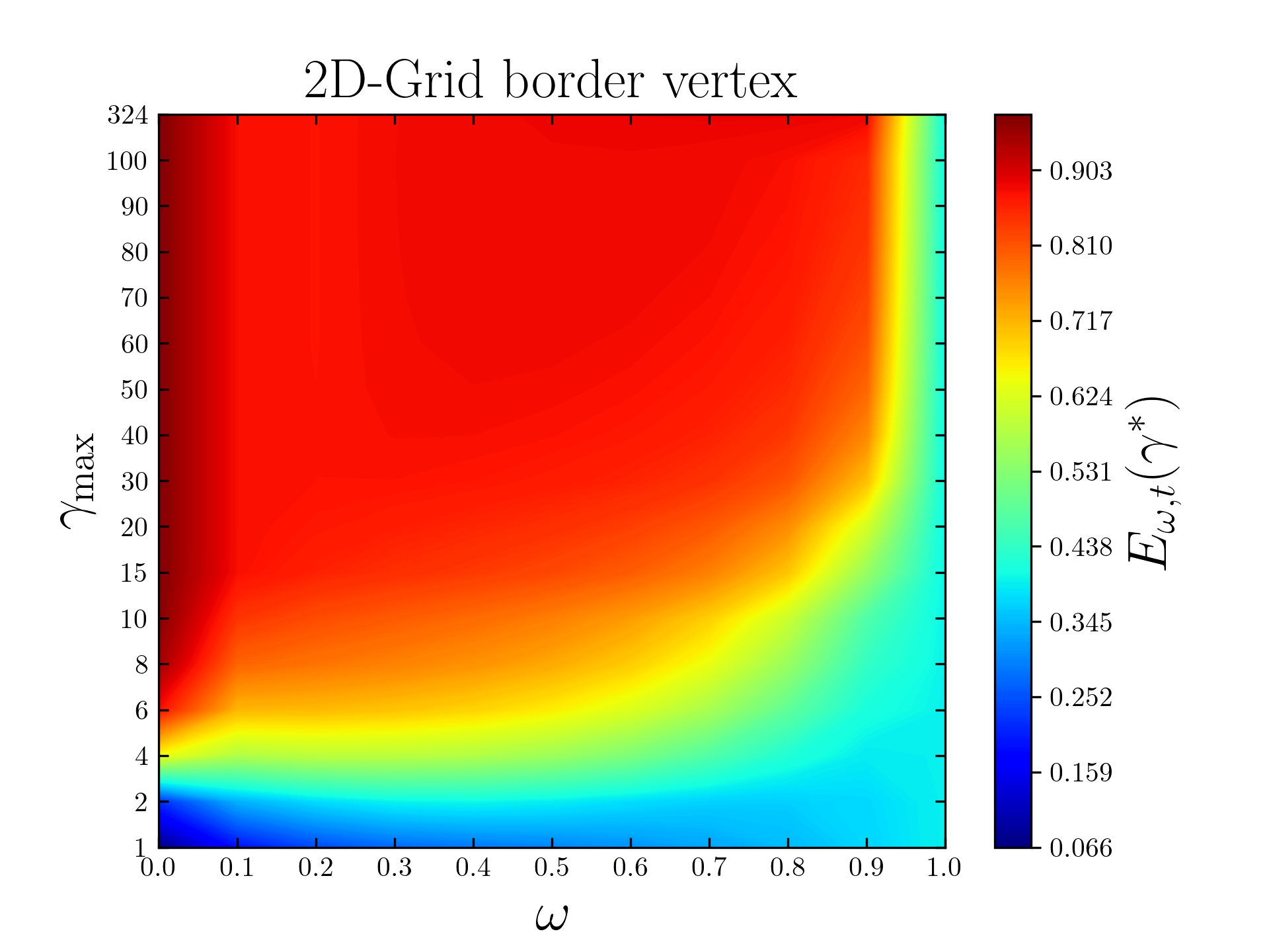
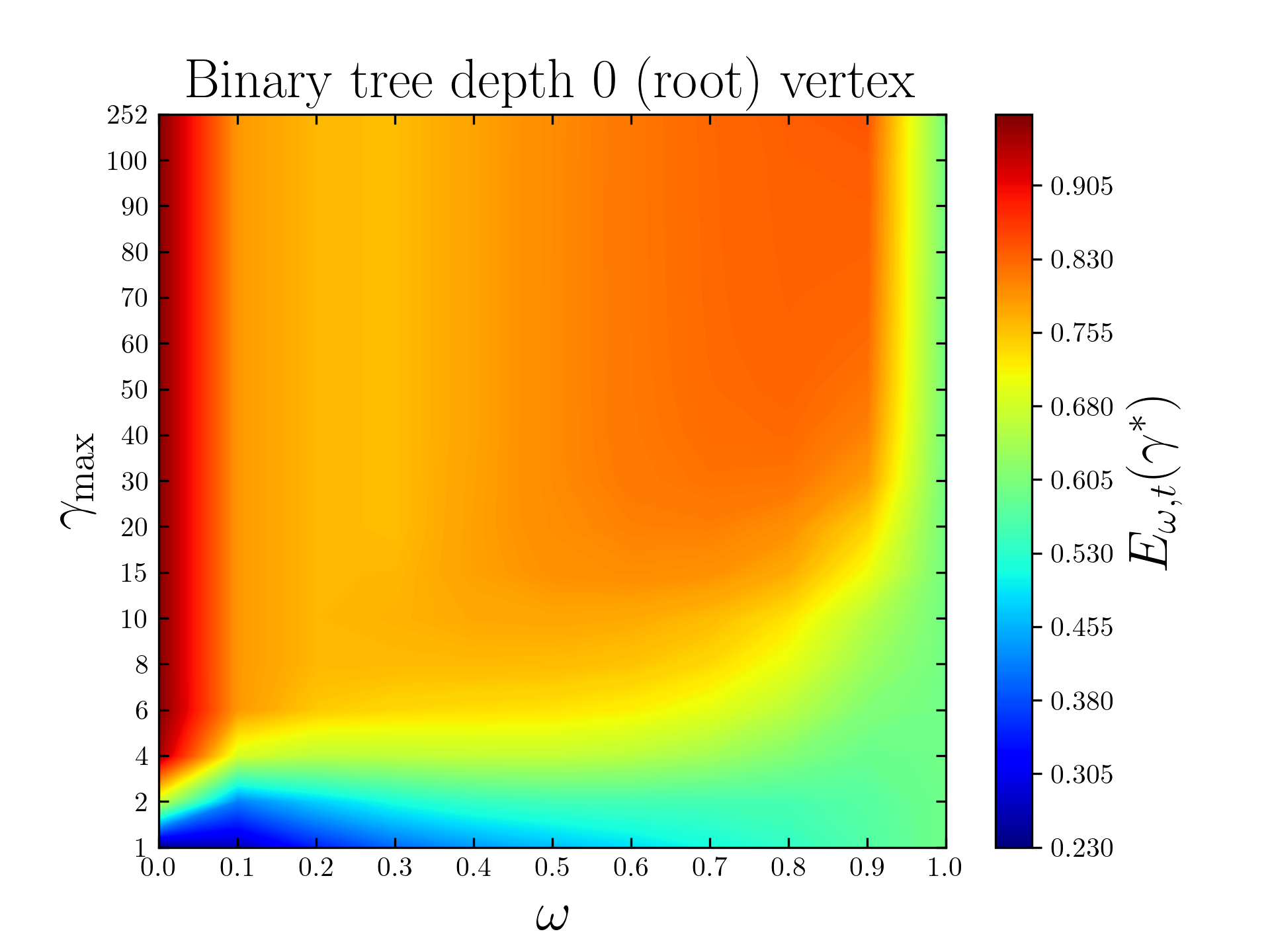
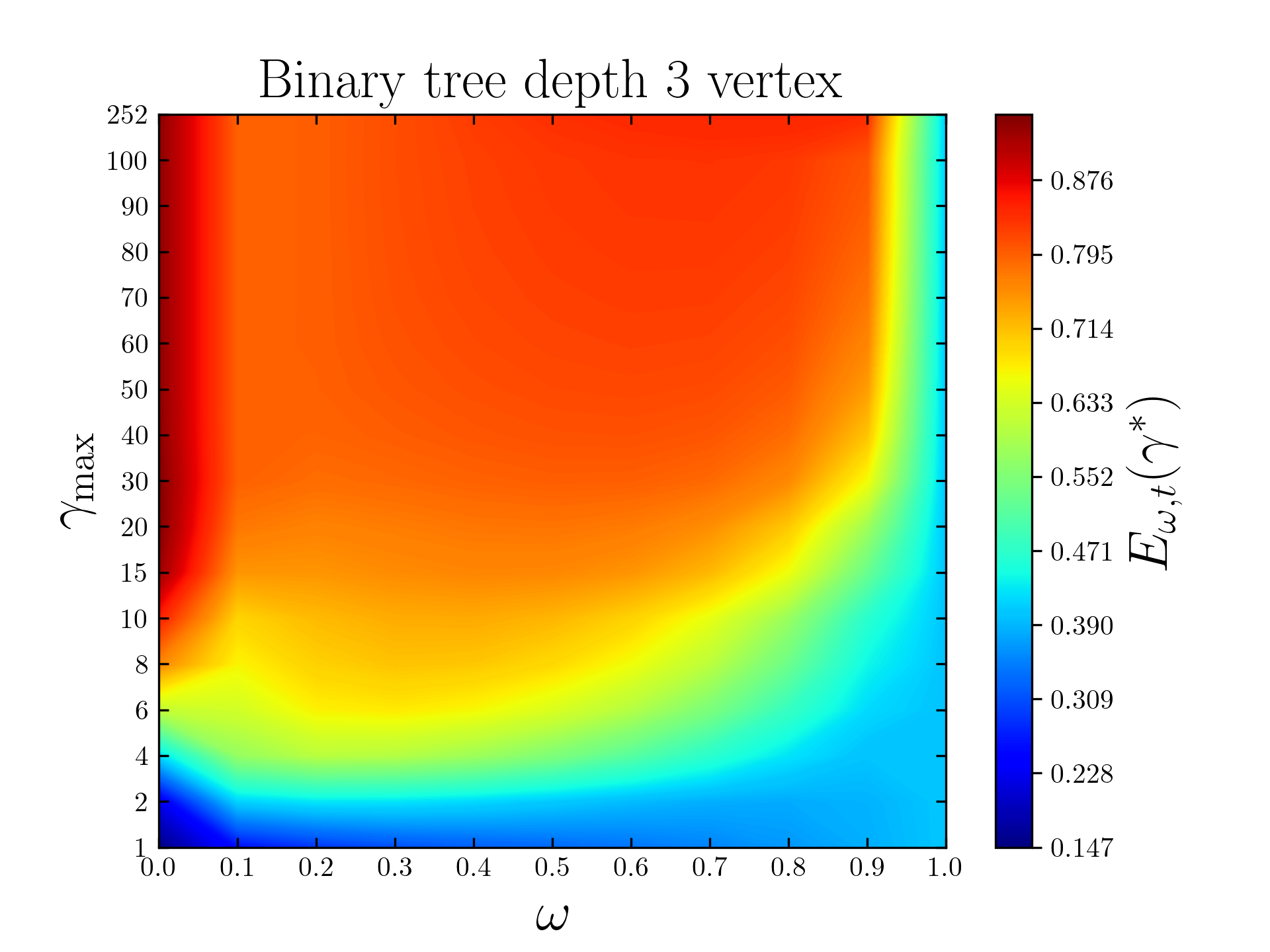
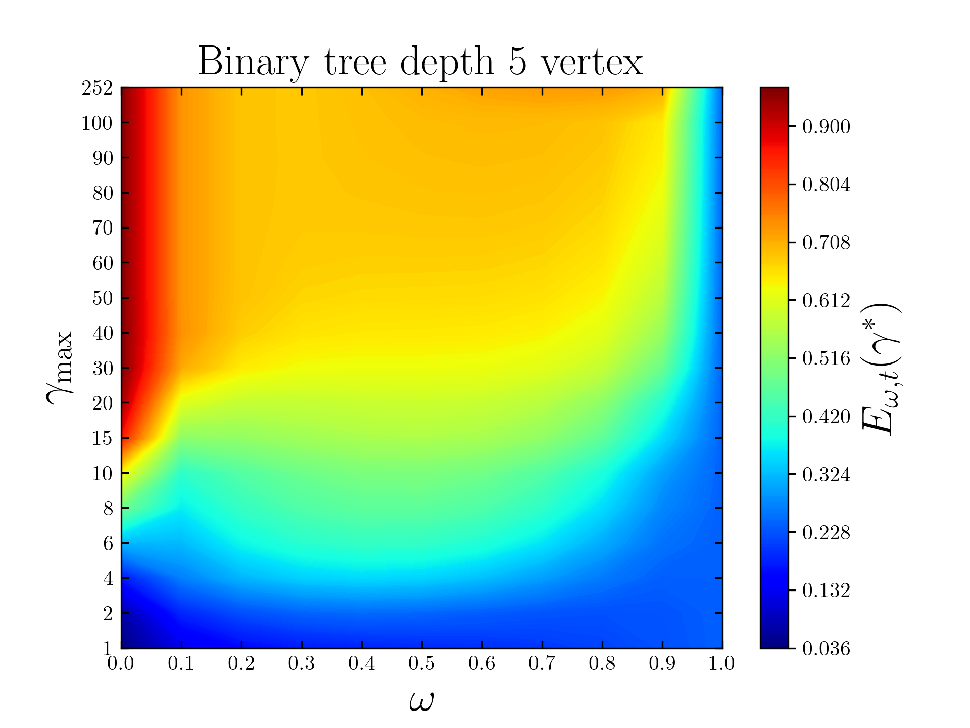
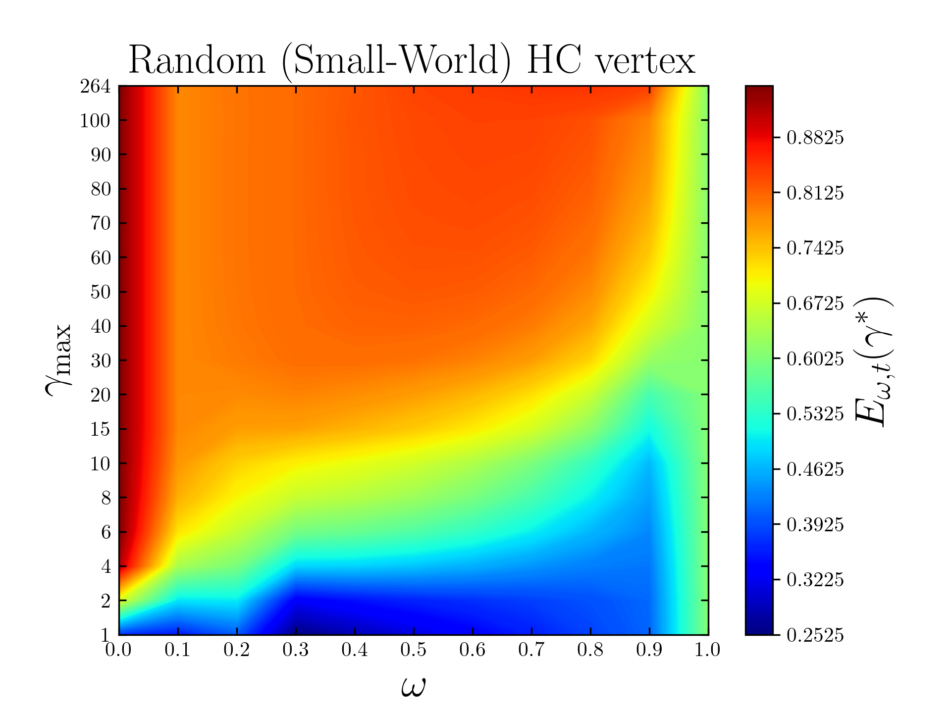
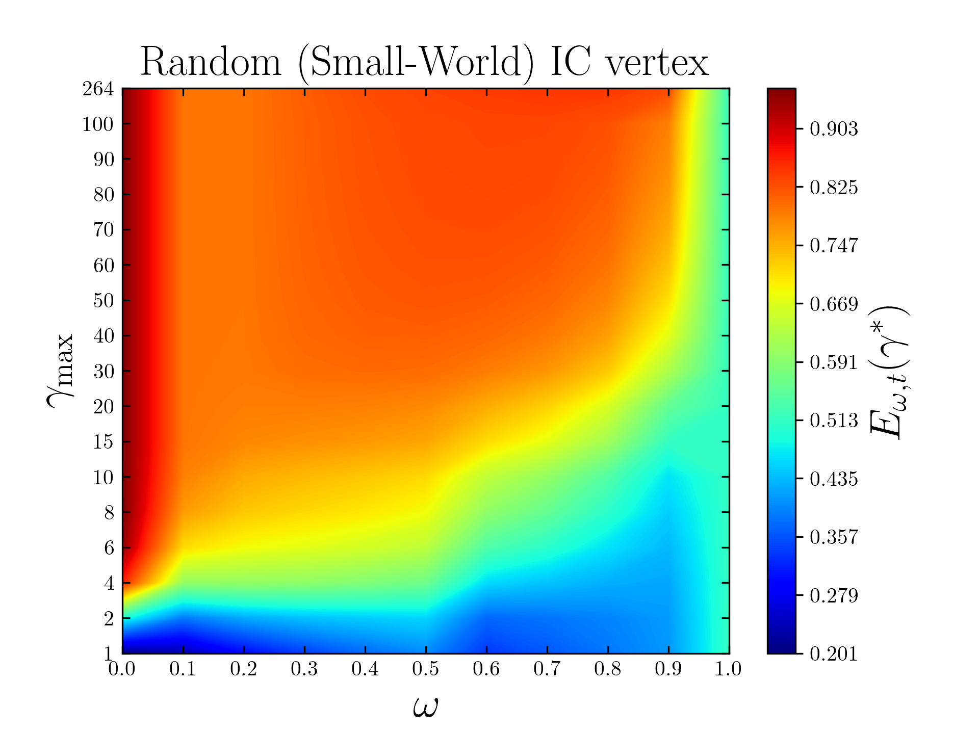
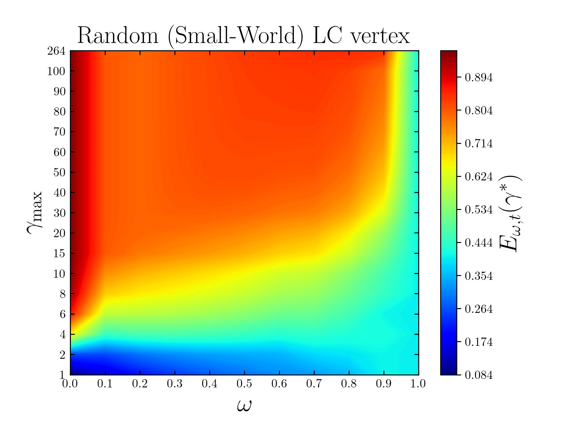
Figure 7: Stochastic Quantum Walk Search (SQWS) performances with restrained value of $\gamma_{\max}\in[1,4N]$ on a maze graph ($M_{73}$), the path graph ($P_{65}$), the star graph ($S_{63}$), the wheel graph ($W_{64}$), the 2D-grid ($G_{9\times 9}$), the perfect binary tree of depth 5 ($PBT_{5}$) and a random graph ($SW_{66}$) which was constructed by gluing together three small-world graphs of size $N=22$ each with different average connectivity and rewiring probabilities. The quantum walk search is recovered for $\omega=0$, the classical random walk search for $\omega=1$, and a linear combination of the two when $\omega\in]0,1[$.

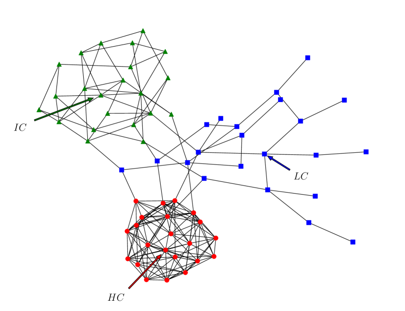
Figure 8: Random graph $SW_{66}$ constructed by gluing together three small-world graphs of size $N=22$ each with different average connectivity and rewiring probabilities. The target vertices are named HC, IC and LC, respectively for high, intermediate and low connectivity. Their average connectivy are respectively 10, 4 and 3. Their respective rewiring probabilities are 0.1, 0.5 and 0.8.

B.2 Ring-lattice transition

As the results on the cycle and the complete graphs are completely different, we use the Ring-lattice graph model to progressively transform a cycle into a complete graph. A ring-lattice graph also known as a $k$-cycle is the basis of Watts and Strogatz model widely known as small-world networks [65]. It consists of a cycle graph where each vertex is connected to its $k$ nearest neighbors. Therefore when $k=2$ we recover a cycle graph and the maximum value of $k$ generates a complete graph. As an illustration we show the transition from the cycle to the complete graph of size $N=8$ in Fig. 9. We run the SQWS on the Ring-lattice graph of size $N=32$ for 16 differents values of $k$, the cycle graph is obtained for $k=2$ and the complete graph for $k=32$. We present the results in Fig. 11. As $k$ increases, the eccentricity of the marked vertex decreases as the graph’s connections increase, leading to an increase in its centrality as shown in Fig. 10. We observe that the hybrid regime outperforms the purely quantum one only for the cycle graph, i.e. $k=2$. A slight increase in connectivity allows the quantum regime to gain the upper hand over the hybrid, as we can see that from $k=4$ the hybrid regime is no more efficient than the purely quantum one for low values of $\gamma_{\max}$. We then note that as the value of $k$ increases, the low-noise hybrid regime, i.e. low value of $\omega$, is less efficient than a noisier hybrid. This feature was clearly visible for the complete $K_{64}$ graph in Fig. 2.

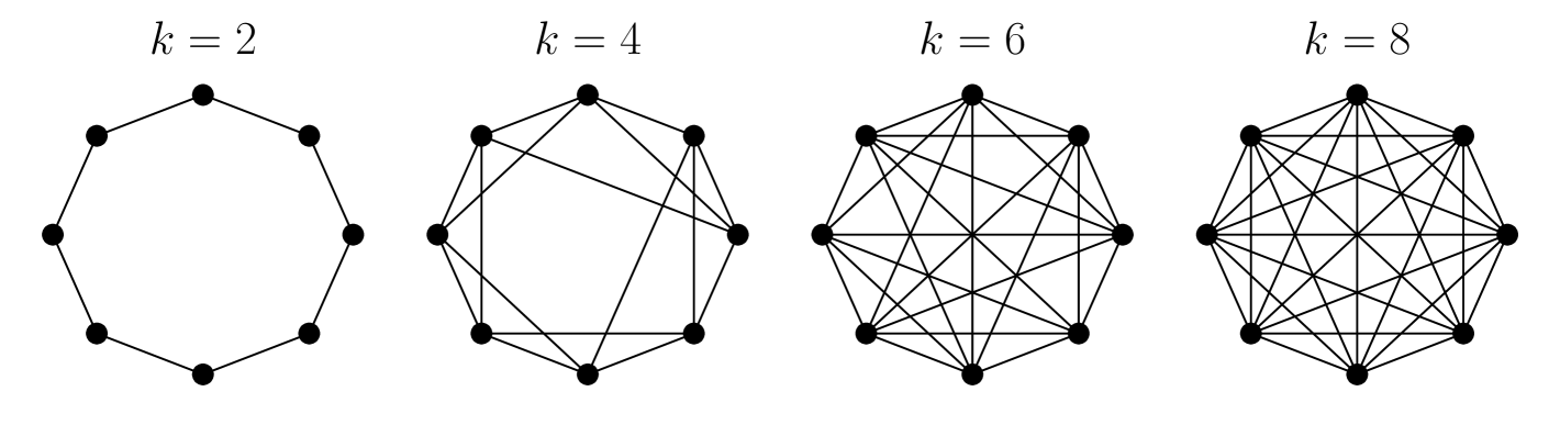
Figure 9: Transition from the cycle graph to the complete graph of size $N=8$ with the Ring-lattice model. As far as possible, each vertex is connected to its $k$-nearest neighbors.

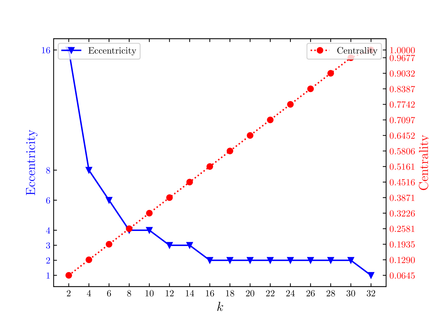
Figure 10: Eccentricity and centrality of the target vertex as a function of $k$ for Ring-lattice graphs of size $N=32$.

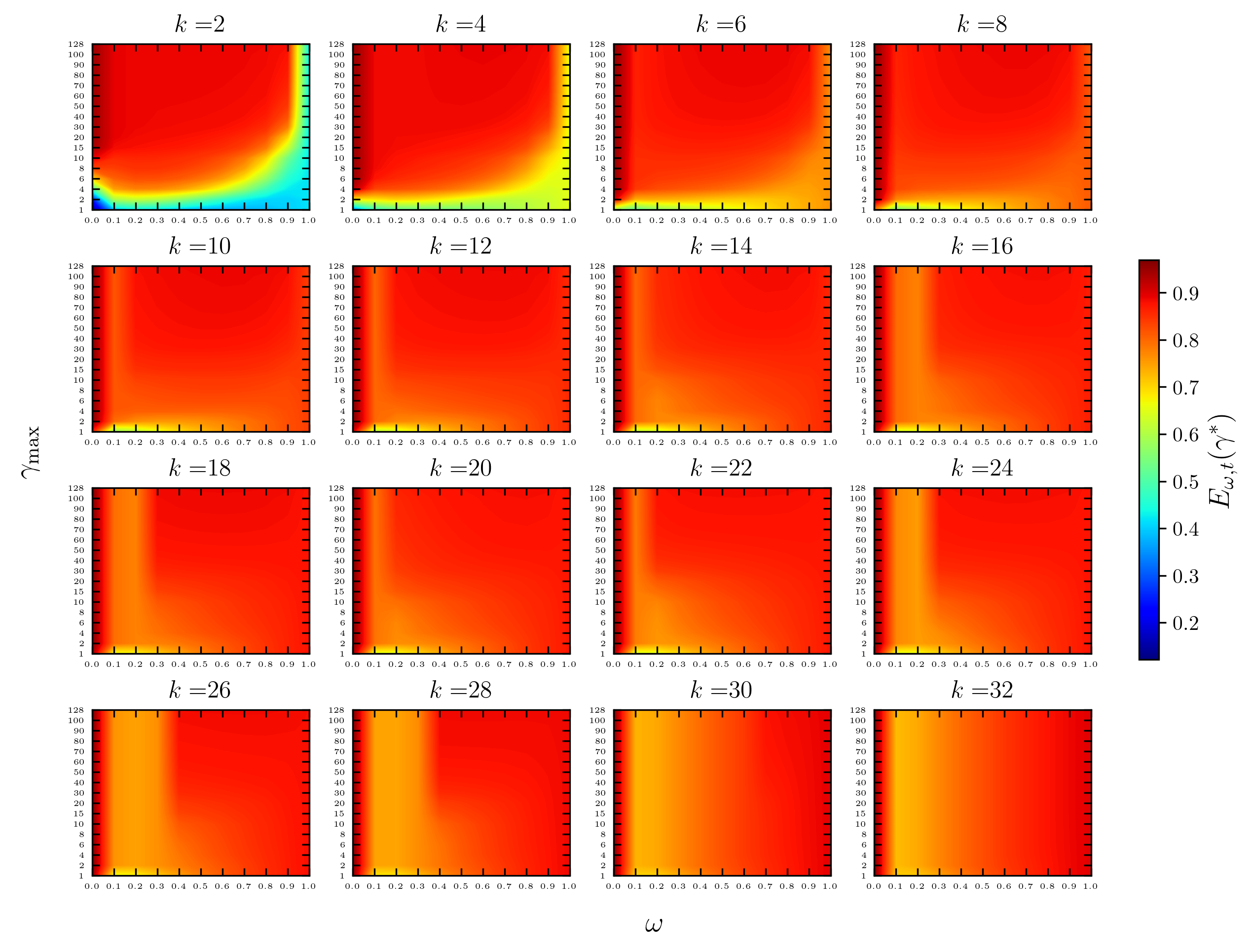
Figure 11: Stochastic Quantum Walk Search (SQWS) performances with restrained value of $\gamma_{\max}\in[1,4N]$ on Ring-lattice graphs of size $N=32$. The cycle graph graph is recovered for $k=2$ and the complete graph for $k=32$. An increase in the value of $k$ corresponds to increasing the average connection of each vertex with its $k$-nearest neighbors. The quantum walk search is recovered for $\omega=0$, the classical random walk search for $\omega=1$, and a linear combination of the two when $\omega\in]0,1[$.

References

- Lovett et al. [2010] N. B. Lovett, S. Cooper, M. Everitt, M. Trevers, and V. Kendon, Physical Review A 81, 042330 (2010).
- Childs [2009] A. M. Childs, Physical Review Letters 102 (2009), ISSN 1079-7114, URL http://dx.doi.org/10.1103/PhysRevLett.102.180501.
- Farhi and Gutmann [1998] E. Farhi and S. Gutmann, Phys. Rev. A 58, 915 (1998), URL https://link.aps.org/doi/10.1103/PhysRevA.58.915.
- Aharonov et al. [1993] Y. Aharonov, L. Davidovich, and N. Zagury, Physical Review A 48, 1687 (1993).
- Bepari et al. [2022] K. Bepari, S. Malik, M. Spannowsky, and S. Williams, Physical Review D 106, 056002 (2022).
- Arnault and Debbasch [2016] P. Arnault and F. Debbasch, Physical Review A 93, 052301 (2016).
- De Nicola et al. [2014] F. De Nicola, L. Sansoni, A. Crespi, R. Ramponi, R. Osellame, V. Giovannetti, R. Fazio, P. Mataloni, and F. Sciarrino, Physical Review A 89, 032322 (2014).
- Di Molfetta et al. [2014] G. Di Molfetta, M. Brachet, and F. Debbasch, Physica A: Statistical Mechanics and its Applications 397, 157 (2014).
- Zylberman et al. [2022] J. Zylberman, G. Di Molfetta, M. Brachet, N. F. Loureiro, and F. Debbasch, Physical Review A 106, 032408 (2022).
- di2 [2016] New Journal of Physics 18, 103038 (2016).
- Eon et al. [2023] N. Eon, G. Di Molfetta, G. Magnifico, and P. Arrighi, Quantum 7, 1179 (2023).
- Sellapillay et al. [2022] K. Sellapillay, P. Arrighi, and G. Di Molfetta, Scientific Reports 12, 2198 (2022).
- Kadian et al. [2021] K. Kadian, S. Garhwal, and A. Kumar, Computer Science Review 41, 100419 (2021).
- Roget and Di Molfetta [2024] M. Roget and G. Di Molfetta, in Asian Symposium on Cellular Automata Technology (Springer, 2024), pp. 72–83.
- Schulz et al. [2024] S. Schulz, D. Willsch, and K. Michielsen, Physical Review Research 6, 013312 (2024).
- Marsh and Wang [2020] S. Marsh and J. B. Wang, Phys. Rev. Res. 2, 023302 (2020), URL https://link.aps.org/doi/10.1103/PhysRevResearch.2.023302.
- Bennett et al. [2021] T. Bennett, E. Matwiejew, S. Marsh, and J. B. Wang, Quantum walk-based vehicle routing optimisation (2021), eprint 2109.14907.
- Slate et al. [2021] N. Slate, E. Matwiejew, S. Marsh, and J. B. Wang, Quantum 5, 513 (2021), ISSN 2521-327X, URL http://dx.doi.org/10.22331/q-2021-07-28-513.
- Campos et al. [2021] E. Campos, S. E. Venegas-Andraca, and M. Lanzagorta, Scientific Reports 11, 16845 (2021).
- Qu et al. [2024] D. Qu, E. Matwiejew, K. Wang, J. Wang, and P. Xue, Quantum Science and Technology 9, 025014 (2024).
- Chang et al. [2023] Y.-J. Chang, W.-T. Wang, H.-Y. Chen, S.-W. Liao, and C.-R. Chang, Preparing random state for quantum financing with quantum walks (2023), eprint 2302.12500, URL https://arxiv.org/abs/2302.12500.
- Choudhury et al. [2024] B. S. Choudhury, M. K. Mandal, and S. Samanta, International Journal of Theoretical Physics 63, 71 (2024).
- Gonzales et al. [2024] A. Gonzales, R. Herrman, C. Campbell, I. Gaidai, J. Liu, T. Tomesh, and Z. H. Saleem, arXiv preprint arXiv:2405.20273 (2024).
- Shi et al. [2024] W.-M. Shi, Q.-T. Zhuang, Y.-H. Zhou, and Y.-G. Yang, Multimedia Tools and Applications 83, 34979 (2024).
- Dernbach et al. [2019] S. Dernbach, A. Mohseni-Kabir, S. Pal, and D. Towsley, in Complex Networks and Their Applications VII: Volume 2 Proceedings The 7th International Conference on Complex Networks and Their Applications COMPLEX NETWORKS 2018 7 (Springer, 2019), pp. 182–193.
- de Souza et al. [2019] L. S. de Souza, J. H. de Carvalho, and T. A. Ferreira, in 2019 8th Brazilian Conference on Intelligent Systems (BRACIS) (IEEE, 2019), URL http://dx.doi.org/10.1109/BRACIS.2019.00149.
- Roget et al. [2022] M. Roget, G. Di Molfetta, and H. Kadri, in Uncertainty in artificial intelligence (PMLR, 2022), pp. 1697–1706.
- Childs et al. [2003] A. M. Childs, R. Cleve, E. Deotto, E. Farhi, S. Gutmann, and D. A. Spielman, in Proceedings of the thirty-fifth annual ACM symposium on Theory of computing (2003), pp. 59–68.
- Chawla et al. [2020] P. Chawla, R. Mangal, and C. M. Chandrashekar, Quantum Information Processing 19, 1 (2020).
- Benedetti and Gianani [2023] C. Benedetti and I. Gianani, AVS Quantum Science 6 (2023).
- Arrighi et al. [2014] P. Arrighi, V. Nesme, and M. Forets, Journal of Physics A: Mathematical and Theoretical 47, 465302 (2014), URL https://dx.doi.org/10.1088/1751-8113/47/46/465302.
- Di Molfetta and Debbasch [2012] G. Di Molfetta and F. Debbasch, Journal of Mathematical Physics 53 (2012).
- Strauch [2006] F. W. Strauch, Physical Review A—Atomic, Molecular, and Optical Physics 73, 054302 (2006).
- Nzongani et al. [2024] U. Nzongani, N. Eon, I. Márquez-Martín, A. Pérez, G. Di Molfetta, and P. Arrighi, Physical Review A 110, 042418 (2024).
- Di Molfetta [2024] G. Di Molfetta, Quantum Walks, Limits, and Transport Equations (IOP Publishing, 2024).
- Jolly and Di Molfetta [2023] N. Jolly and G. Di Molfetta, The European Physical Journal D 77, 80 (2023).
- Grover [1996] L. K. Grover, in Proceedings of the twenty-eighth annual ACM symposium on Theory of computing (1996), pp. 212–219.
- Zalka [1999] C. Zalka, Physical Review A 60, 2746 (1999).
- Roget et al. [2020] M. Roget, S. Guillet, P. Arrighi, and G. Di Molfetta, Physical Review Letters 124, 180501 (2020).
- Stoudenmire and Waintal [2024] E. M. Stoudenmire and X. Waintal, Phys. Rev. X 14, 041029 (2024), URL https://link.aps.org/doi/10.1103/PhysRevX.14.041029.
- Shenvi et al. [2003] N. Shenvi, J. Kempe, and K. B. Whaley, Physical Review A 67, 052307 (2003).
- Childs and Goldstone [2004] A. M. Childs and J. Goldstone, Physical Review A 70, 022314 (2004).
- Ambainis et al. [2020] A. Ambainis, A. Gilyén, S. Jeffery, and M. Kokainis, in Proceedings of the 52nd Annual ACM SIGACT Symposium on Theory of Computing (2020), pp. 412–424.
- Apers et al. [2022] S. Apers, S. Chakraborty, L. Novo, and J. Roland, Physical review letters 129, 160502 (2022).
- Whitfield et al. [2010] J. D. Whitfield, C. A. Rodríguez-Rosario, and A. Aspuru-Guzik, Physical Review A 81 (2010), ISSN 1094-1622, URL http://dx.doi.org/10.1103/PhysRevA.81.022323.
- Benjamin and Dudhe [2024] C. Benjamin and N. Dudhe, Journal of Statistical Mechanics: Theory and Experiment 2024, 013402 (2024).
- Mart´ınez-Mart´ınez and Sánchez-Burillo [2016] I. Martínez-Martínez and E. Sánchez-Burillo, Scientific reports 6, 23812 (2016).
- Dalla Pozza and Caruso [2020] N. Dalla Pozza and F. Caruso, Physics Letters A 384, 126195 (2020), ISSN 0375-9601, URL http://dx.doi.org/10.1016/j.physleta.2019.126195.
- Wang et al. [2022] L.-J. Wang, J.-Y. Lin, and S. Wu, Physical Review Research 4, 023058 (2022).
- Schuhmacher et al. [2021] P. K. Schuhmacher, L. C. Govia, B. G. Taketani, and F. K. Wilhelm, Europhysics Letters 133, 50003 (2021).
- Tang et al. [2019] H. Tang, Z. Feng, Y.-H. Wang, P.-C. Lai, C.-Y. Wang, Z.-Y. Ye, C.-K. Wang, Z.-Y. Shi, T.-Y. Wang, Y. Chen, et al., Physical Review Applied 11, 024020 (2019).
- Ding et al. [2024] Z. Ding, X. Li, and L. Lin, PRX Quantum 5, 020332 (2024).
- Caruso [2014] F. Caruso, New Journal of Physics 16, 055015 (2014), ISSN 1367-2630, URL http://dx.doi.org/10.1088/1367-2630/16/5/055015.
- Caruso et al. [2016] F. Caruso, A. Crespi, A. G. Ciriolo, F. Sciarrino, and R. Osellame, Nature Communications 7 (2016), ISSN 2041-1723, URL http://dx.doi.org/10.1038/ncomms11682.
- Pozza et al. [2021] N. D. Pozza, L. Buffoni, S. Martina, and F. Caruso, Quantum reinforcement learning: the maze problem (2021), eprint 2108.04490.
- Matsuoka et al. [2024] L. Matsuoka, H. Ohno, and E. Segawa, arXiv preprint arXiv:2411.12191 (2024).
- Mülken and Blumen [2011] O. Mülken and A. Blumen, Physics Reports 502, 37 (2011).
- Wong [2022] T. G. Wong, Quantum Information and Computation 22, 53–85 (2022), ISSN 1533-7146, URL http://dx.doi.org/10.26421/QIC22.1-2-4.
- Chakraborty et al. [2016] S. Chakraborty, L. Novo, A. Ambainis, and Y. Omar, Physical review letters 116, 100501 (2016).
- Chakraborty et al. [2020] S. Chakraborty, L. Novo, and J. Roland, Physical Review A 102, 032214 (2020).
- Malmi et al. [2022] J. Malmi, M. A. Rossi, G. García-Pérez, and S. Maniscalco, Physical review research 4, 043185 (2022).
- Delahaye et al. [2019] D. Delahaye, S. Chaimatanan, and M. Mongeau, Handbook of metaheuristics pp. 1–35 (2019).
- Johansson et al. [2012] J. Johansson, P. Nation, and F. Nori, Computer Physics Communications 183, 1760–1772 (2012), ISSN 0010-4655, URL http://dx.doi.org/10.1016/j.cpc.2012.02.021.
- Hagberg et al. [2008] A. Hagberg, P. J. Swart, and D. A. Schult, Tech. Rep., Los Alamos National Laboratory (LANL), Los Alamos, NM (United States) (2008).
- Watts and Strogatz [1998] D. J. Watts and S. H. Strogatz, nature 393, 440 (1998).