A mesh-free hybrid Chebyshev-Tucker tensor format with applications to multi-particle modelling
Abstract
In this paper, we introduce a mesh-free two-level hybrid Tucker tensor format for approximation of multivariate functions, which combines the product Chebyshev interpolation with the ALS-based Tucker decomposition of the tensor of Chebyshev coefficients. It allows to avoid the expenses of the rank-structured approximation of function-related tensors defined on large spacial grids, while benefiting from the Tucker decomposition of the rather small core tensor of Chebyshev coefficients. This leads to nearly optimal Tucker rank parameters which are close to the results for well established Tucker-ALS algorithm applied to the large grid-based tensors. These rank parameters inherited from the Tucker-ALS decomposition of the coefficient tensor can be much less than the polynomial degrees of the initial Chebyshev interpolant via function independent basis set. Furthermore, the tensor product Chebyshev polynomials discretized on a tensor grid leads to a low-rank two-level orthogonal algebraic Tucker tensor that approximates the initial function with controllable accuracy. It is shown that our techniques could be gainfully applied to the long-range part of the electrostatic potential of multi-particle systems approximated in the range-separated tensor format. Error and complexity estimates of the proposed methods are presented. We demonstrate the efficiency of the suggested method numerically on examples of the long-range components of multi-particle interaction potentials generated by 3D Newton kernel for large bio-molecule systems and lattice-type compounds.
Key words: Tensor numerical methods, Chebyshev interpolation, multilinear algebra, multi-particle electrostatic potentials, Tucker and canonical tensor formats.
AMS Subject Classification: 65F30, 65F50, 65N35, 65F10
1 Introduction
Tensor numerical methods (TNM) intrinsically reduce the numerical solution of multidimensional problems to one-dimensional calculations. In recent years, TNM are proven to be a powerful tool for solving numerically intensive multi-dimensional problems in scientific computing arising in computational quantum chemistry [33, 26], multi-dimensional dynamical problems, data science, stochastic simulations, optimal control problems, etc., see, e.g., [30]. The benefits of the TNM for -dimensional problems are due to the reduction of both computational and storage complexity to merely linear scaling in . Other approaches for optimizing numerical algorithms can be based on the concept of model reduction, see, e.g., [3, 6] and references therein.
Tensor numerical methods provide the bridging of approximation theory for multi-dimensional functions and operators from one side and the modern multilinear algebra techniques from the other side. The construction of efficient TNM is guided by the trade-off between approximation accuracy and computational complexity of the chosen nonlinear rank-structured approximation algorithms, while taking into account the compatibility of the resultant tensor representations with available multilinear algebra. The total numerical complexity of tensor approximations is a sum of the high computational cost for (a) the algebraic operations of nonlinear low-rank approximation of multidimensional functions and operators in the traditional canonical (CP) [23], Tucker [49], tensor train (TT) [39], quantized tensor train (QTT) [29] or range-separated (RS) [4] tensor formats, and (b) the cost of function evaluations required for implementation of the tensor algorithms. Thereafter, the overall approximation accuracy can be controlled by tensor rank parameters as well as the precision of the chosen functional approximations (given the storage budget, accuracy is limited by the data regularity). A number of recent developments confirm efficiency of TNM in different research fields [47, 41, 35, 34, 44, 1, 43, 50].
TNM are usually applied to grid-based rank-structured tensor approximation of target functions and operators, discretized on large spacial grids in with , for the numerical solution of large scale scientific computing problems, see [30, 26, 5]. Alternatively, classical mesh-free approximation methods for functions are based on their representation in problem-independent sets of functions, such as trigonometric functions (Fourier basis), (piecewise) polynomials, Sinc functions or Gaussians, [45, 48, 10, 38, 35, 18], as well as fast multipole methods [19].
This paper is motivated by recent advances in low-rank tensor techniques for tensor product Chebyshev interpolation [2, 16, 17, 22, 46]. Chebyshev polynomials [12] are among the most commonly used set of interpolating functions due to many beneficial features [8, 7, 38]. Error analysis for tensor product interpolation by Chebyshev polynomials was presented for example in [20]. MATLAB implementations of the Chebyshev interpolation method in 1D and 3D (chebfun and chebfun3) are available [48, 17, 22].
The basic version of chebfun3 applies to the input functions presented in the form of canonical tensor format, thus using chebfun for 1D polynomial interpolation. Approximation of the target function in a separable form in 3D [22] is performed via a variant of the heuristic method adaptive cross approximation (ACA) [2] that combines ACA for the 2D slices with agglomeration of slices along the third spacial direction. Hence, the number of functional calls in such an approach is a multiple of polynomial degrees , the CP rank of ACA approximation on each slice, , and the number of slices, . This procedure may reduce the number of functional calls under the condition . In turn, the direct tensor-product Chebyshev interpolant requires functional calls. The modification of Chebfun3 algorithm that reduces the number of functional calls was presented in [16].
In general, for functions of continuous arguments, one can apply mesh-free interpolation-type approximations in the form of a weighted sum of a given problem independent set of functions (not necessary orthogonal), where the corresponding weights require the values of the target function only at a few predefined interpolation points in a computational domain. This usually leads to asymptotically quasi-optimal accuracy for each particular input function having good smoothness characteristics. However, for functions with low regularity, satisfactory accuracy may require a rather large set of interpolating functions, say, with in the range of many hundreds if not thousands, which makes further use of such interpolants in scientific computing non-tractable. That is the main bottleneck for interpolation of multivariate functions by Chebyshev polynomials.
In this paper, we introduce and analyze a novel method for approximating multivariate functions by using Chebyshev polynomial interpolation in with , which combines the tensor product Chebyshev polynomial interpolation in the global computational domain with the ALS-based Tucker decomposition of the rather small tensor of Chebyshev coefficients111Using the non-orthogonal interpolating functions leads to small modification of the computational scheme.. This leads to the construction of mesh-free two-level Tucker tensor format for approximation of multivariate functions, either given explicitly or only available on a regular grid. It allows to avoid the expenses of the rank-structured approximation of function-related tensors defined on large spacial grids, while benefiting from the Tucker decomposition of the rather small core tensor of Chebyshev coefficients, which leads to nearly optimal rank parameters as for the well established grid-based methods. The ranks inherited from the Tucker-ALS decomposition are almost optimal and can be much less than the polynomial degree of the initial Chebyshev interpolant which is chosen independent of the grid sizes in grid-based methods. Thus, we compute the nearly optimal Tucker decomposition of the 3D function without discretizing the function on the full grid in the computational domain, but only using its values at Chebyshev nodes. Finally, we can represent the function in Tucker format with the optimal -rank on an arbitrarily large 3D tensor grid in the whole computational domain by discretizing the Chebyshev polynomials on that grid. Note that in the case of functions with multiple cusps (or even stronger singularities), our method applies to the long-range component of the target function approximated in the range-separated (RS) tensor format [4].
We underline that, given accuracy , our main goal in this paper is to construct numerical methods that allow to compute the mesh-free Tucker tensor approximation of the target function with almost optimal tensor rank which is usually much smaller than the Chebyshev polynomials degree that guarantees the accuracy . In turn, the parameter should be much smaller than the grid size that is required for -accurate grid-based discretizations with the mesh-size ,
| (1.1) |
The Tucker rank of the output tensor is the most important parameter for the complexity characteristics of subsequent multilinear tensor calculus in respective applications.
We present numerical experiments demonstrating the efficiency of the proposed techniques on nontrivial examples, including the computation of multi-particle electrostatic potentials arising in bio-molecular modelling and lattice type structure calculations in material science. In particular, it is gainfully applied to the long-range part of the many-particle electrostatic potentials in , obtained by the RS tensor format [4]. Numerical results indicate that the low-rank tensor representations can be computed with controllable accuracy such that the numerical cost depends weakly on the size of the many-particle system [4]. On the other hand, our numerics reproduce the earlier results obtained by the grid-based tensor numerical methods [31, 25]. In summary, we state the main benefits of the proposed method as follows:
-
•
Fast and accurate quasi-optimal mesh-free Tucker tensor decomposition of regular functions with rather small number of Chebyshev polynomials.
-
•
Efficient quasi-optimal mesh-free Tucker decomposition of the long-range part of the multi-particle electrostatic potential, i.e., the large weighted sum of Newton kernels.
-
•
In case of input function presented in the canonical (CP) tensor format our method needs only a small number of 1D-Chebyshev interpolation of canonical skeleton vectors.
The remainder of the paper is organized as follows. In Section 2, we describe the definition and construction of our mesh-free hybrid Chebychev-Tucker tensor representation. We discuss here transforming of the hybrid representation to the standard low-rank Tucker format. Section 3 presents the numerical schemes for the hybrid Chebyshev-Tucker approximation of trivariate functions, either given explicitly or only available on a regular grid. The corresponding theorems on error and complexity bounds of the Chebyshev-Tucker approximation conclude this section. Section 4 first outlines the techniques for grid-based low-rank tensor representations of multi-particle interaction potentials. We then discuss in details the Chebyshev-Tucker approximation of trivariate functions with singularities (the Newton kernel). We show efficiency of our methods for approximating the long-range part of the multi-particle electrostatic potentials of bio-molecular systems of different size, and present various numerical tests illustrating the performance of the proposed approach. Numerical results for application of the new method to lattice-type compounds are also presented in this section. Finally, Section 5 concludes the paper and outlines the future research directions.
2 The mesh-free hybrid Chebychev-Tucker tensor format
In this section, we review the basics of tensors and introduce the hybrid Chebyshev-Tucker tensor format for the approximation of multivariate functions.
2.1 Definition of hybrid tensor format
Recall that a tensor of order is defined as a real multidimensional array over a -tuple index set
| (2.1) |
with multi-index notation , . It is considered as an element of the Euclidean vector space . To get rid of the exponential scaling in storage size and the consequent drawbacks, one can apply the rank-structured formatted separable approximations of multidimensional tensors.
The -term canonical (CP) tensor format is defined by a finite sum of rank-1 tensors
| (2.2) |
where are normalized vectors, and is the canonical rank. We also call the vectors the canonical vectors.
Recall that the rank-, , orthogonal Tucker format is specified as the set of tensors parametrized as follows,
| (2.3) |
where is the set of orthonormal vectors for . Here denotes the contraction product along the mode with the orthogonal matrices . The Tucker core tensor is denoted by .
Next, we define the functional analog of the Tucker format, which we call the functional Tucker format.
Definition 2.1 (Functional Tucker format).
We say that the real-valued function defined on is represented in the functional rank- Tucker format if it allows the factorization
| (2.4) |
where is the core tensor and is the Tucker factor function defined as a vector-valued function with functional entries, i.e., for , , .
In the following definition we distinguish the discrete and functional two-level hybrid tensor formats formulated for the three-dimensional case, .
Definition 2.2 (Two-level hybrid Tucker formats).
(A) (Functional case) If the core tensor in Eq. 2.4 is in turn a rank- Tucker tensor,
| (2.5) |
then we call is represented in the two-level hybrid functional rank- Tucker format.
(B) (Algebraic case). We say that tensor is parametrized in the two-level hybrid rank- Tucker-Tucker algebraic format if it admits the representation
| (2.6) |
where the core coefficient is given by the rank- Tucker tensor with the small Tucker ranks .
Furthermore, if the functional entries of in Eq. 2.4 are specified by the Chebyshev polynomials, we say that the function is represented in the (two-level hybrid) Chebychev-Tucker format, shortly ChebTuck format. See Definition 2.3 below.
Definition 2.3 (ChebTuck format).
Let denote the -th Chebyshev polynomial of the first kind on , which forms a sequence of orthogonal polynomials on with respect to the weight . Let denote the vector-valued function of the first Chebyshev polynomials. We say that the real-valued function defined on is represented in the ChebTuck- format if it allows the factorization
| (2.7) |
where is a rank- Tucker tensor given by
| (2.8) |
For the practical application of the presented hybrid Tucker-type tensor representation in scientific computing, one requires the implementation of the standard multilinear algebra operations within arising tensor calculus. This means that tensors in hybrid format might be easily transformed to the standard Tucker-type format when required. This issue will be considered in the following Section 2.2.
2.2 Transforming hybrid representation to the standard low-rank Tucker format
The following Proposition 2.4 proves that any tensor parametrized as the two-level orthogonal Tucker format with ranks can be converted to the standard Tucker tensor with the reduced (quasi-optimal) rank parameters . This allows the traditional multilinear algebra operations with the tensors in the hybrid format. Moreover, the resultant Tucker tensor can be transformed to a canonical format with small rank.
Proposition 2.4.
Let the two-level third order orthogonal Tucker tensor be given in the form Eq. 2.3, where the core coefficient is parametrized by the rank orthogonal Tucker tensor
| (2.9) |
with the core tensor . Then the initial tensor takes the form of a rank orthogonal Tucker representation
| (2.10) |
with the core tensor and the orthogonal Tucker factor matrices .
Proof.
Notice that if Eq. 2.9 represents a non-orthogonal Tucker tensor, then appear to be the non-orthogonal matrices, also that the resultant conventional Tucker tensor (2.10) can be easily transformed to the canonical tensor format by using the so-called Tuck-to-can transform, see [31, Def. 2.3, (2.6)], [28, Rem. 2.7], and [26]. This Tuck-to-can algorithm will be applied to the core tensor in Eq. 2.9.
The following statement is important in further use of the hybrid functional representation in multilinear algebra, see also (3.9).
Proposition 2.5.
The representation Eq. 2.7 can be converted to the standard functional Tucker format as in Definition 2.1, i.e., Eq. 2.7 can be equivalently written as
| (2.12) |
where the Tucker factor functions are given by , i.e., each entry of is a linear combination of the Chebyshev polynomials. If Eq. 2.9 present the orthogonal Tucker tensor, then appear to be the set of orthogonal polynomials.
The proof of this proposition is in essence the same as the proof of Proposition 2.4, i.e., follows directly from the definition of contracted product operations . However, here we provide a detailed proof to write out several useful equivalent representations of the ChebTuck format explicitly.
Proof.
From Eq. 2.7 we have
| (2.13) | ||||
where for . The desired result then follows. The orthogonality property is based on the argument analogues to the algebraic case but reformulated for polynomial arrays and note that the inner product should be properly weighted. ∎
Remark 2.6.
From the equivalent representations Eq. 2.13 of the ChebTuck format, we can see that it is a degree polynomial in Chebyshev basis, where the coefficients are given as a Tucker tensor. For this reason, we sometimes also write a subscript to denote the ChebTuck format of certain degrees, e.g., .
3 Numerical schemes for hybrid Chebyshev-Tucker approximation of trivariate functions
In what follows, we introduce the numerical schemes for rank-structured approximation of trivariate functions in the novel ChebTuck tensor format introduced in Definition 2.3. The basic idea is to first compute the Chebyshev coefficient tensor , either in full tensor format or in some low-rank format, and then convert to the desired Tucker format with quasi-optimal -rank. Our techniques can be applied directly to multivariate functions with moderate regularity for which the Chebyshev tensor product interpolation demonstrates satisfactory convergence rates. Furthermore, we extend the presented approach beyond the class of regular functions and successfully apply it to functions with multiple singularities by using the range-separated tensor decomposition.
3.1 Classical multivariate Chebyshev interpolant
3.1.1 Functional case
Given a function , we consider its approximation by the tensor product of Chebyshev polynomials in the form (c.f. Eq. 2.7)
| (3.1) |
where is the -th Chebyshev polynomial of the first kind, is the Chebyshev coefficient tensor and is the degree of the Chebyshev polynomials in each mode.
There are mainly two ways to view the approximant which leads to two different methods to compute the Chebyshev coefficient tensor . The first way is to view as a truncation of the tensor product Chebyshev series expansion of and compute the coefficients by projection and integration. The analytic expressions for the Chebyshev coefficients in this case are straightforward to derive. In fact, each coefficient is a -weighted inner product of and the corresponding Chebyshev basis, i.e.,
| (3.2) |
see e.g., [36, 37], but the computation is troublesome since one needs to evaluate those 3-dimensional integrals. The second way is to view as an interpolation of at Chebyshev nodes, namely, satisfies the following interpolation property
| (3.3) |
where are the Chebyshev nodes of the second kind on each mode given by
| (3.4) |
The derivation of the Chebyshev coefficient tensor in this case is more involved while it turns out that the computation can be done efficiently by the discrete cosine transform (DCT). The accuracy of these two approaches is normally similar [36] and we will therefore focus on the interpolation approach in this paper. See also [46, 16, 22].
For this purpose, we first define the function evaluation tensor of at Chebyshev nodes as
| (3.5) |
and the DCT matrix as
| (3.6) |
then somewhat surprisingly, by [38, Equations 6.27-6.28], the Chebyshev coefficient tensor can be computed by the DCT of the function evaluation tensor as
| (3.7) |
Given an error tolerance , we can approximate the coefficient tensor by a Tucker tensor with almost optimal rank parameter using Tucker-ALS algorithm denoted by
| (3.8) |
with and , . See Remark 3.1 for the discussions on Tucker-ALS and other Tucker decomposition algorithms. Substituting in Eq. 3.1 by its Tucker format Eq. 3.8 gives the ChebTuck approximation of , denoted by . In view of Proposition 2.5, the ChebTuck approximation of can be written as
| (3.9) |
where for , .
In summary, this leads to the following straightforward Algorithm 1 for constructing the Chebyshev-Tucker approximation of a function .
Remark 3.1.
It is important to note that tuck_als in 4 of Algorithm 1 can be any Tucker decomposition algorithm that can approximate a tensor in Tucker format with almost optimal rank parameters. Tucker-ALS [14, 15] is the classical algorithm for this purpose and is widely used in practice. It enjoys strong theoretical guarantees such that for any given , it can approximate the original tensor in the sense of relative error with almost optimal rank parameters, where is the Frobenius norm of a tensor. However, it is computational expensive since it requires the access to all entries of the tensor , amounting to space complexity and successive SVDs of the unfolding matrices, amounting to algebraic operations. Alternatives to the classical Tucker-ALS are, e.g., the multigrid algorithm [31], cross-based algorithms [40, 16, 42, 22], or randomized algorithms [11, 32]. In case of the relatively small rank of the input tensor, those algorithms are more efficient in terms of computational cost and memory usage, but they may contain several heuristics, especially the cross-based algorithms with no theoretical accuracy guarantees for given . The discussions on the difference and choice of Tucker decomposition algorithms are beyond the scope of this paper. We use the classical Tucker-ALS algorithm in our theoretical analysis and numerical experiments demonstrated reliable efficiency for low-rank approximation of the coefficients tensor .
3.1.2 Algebraic case with full tensor input
In many applications, see [30, 26, 5] among others, including ours on multi-particle modelling which will be discussed in Section 4, the function may not be given explicitly in the full domain , but only the data on equi-spaced grid are available. Specifically, we only have access to the function values at the uniform grid points collected in a tensor
| (3.10) |
where is the grid point and is the grid size.
In this case, to obtain the function values at Chebyshev nodes, we first construct a multivariate cubic spline interpolation of the data on the uniform grid, i.e., , and then evaluate at Chebyshev nodes, as shown in Algorithm 2. The rest of the algorithm remains the same as Algorithm 1. Note that here and forehand, we assume naturally to ensure the existence of the cubic spline.
3.1.3 Algebraic case with CP tensor input
In fact, the multivariate cubic spline interpolation, see e.g. [13, Chapter 17], is expensive in terms of computational cost. However, in many applications of interest, e.g., quantum chemistry [26], multi-particle modelling [30] and the discretization of certain differential operators [24], the target input tensor has some inherent low-rank structure and thus can be cheaply represented in some low-rank tensor format. In such cases, the computation of the evaluation tensor can be done more efficiently. In particular, we consider here the case where is given in the CP format, i.e.,
| (3.11) |
where are normalized canonical vectors of each mode. In this case, we only need to construct univariate cubic spline interpolations of the canonical vectors in each mode and make tensor products and summations of them. Specifically, let be the cubic spline of the data on the uniform grid , i.e., and then construct the sum of the tensor product of the univariate splines as
| (3.12) |
Finally, the function evaluation tensor can be obtained by evaluating at Chebyshev nodes. The rest of the algorithm remains the same as Algorithm 1. This procedure is summarized in Algorithm 3.
In the case of CP tensor input, one can do better than the above Algorithm 3 by avoiding the construction of the function evaluation tensor then computing the Chebyshev coefficients directly by Eq. 3.7, which requires storage where we assume . In fact, the function evaluations in Algorithm 3 also admits a CP representation given by
| (3.13) |
where contains the function evaluations of the univariate spline at , i.e., . Therefore, the Chebyshev coefficient tensor can be computed directly by Eq. 3.7 as
| (3.14) |
where for . From here, we can leverage the reduced HOSVD (RHOSVD) [31] method instead of full tuck_als to compress directly from canonical to Tucker format, without forming the full tensor . The rest of the algorithm remains the same as Algorithm 1. This procedure is summarized in Algorithm 4.
Remark 3.2.
(Mesh-free method) Our Algorithms outline the computational schemes for low-rank tensor approximation of the function in both the functional and algebraic (discrete) cases. We underline that in both cases our Algorithms are implemented as mesh-free computational schemes in the sense that one needs only access to the functional values on the Chebyshev interpolation grid in 3D (in general, approximate values), but does not require storage of the discretized function on the fine 3D-grid and further computing the Tucker approximation of arising large 3D tensor array by using the Tucker-ALS scheme or by other means (as for the traditional grid based tensor approximation methods). Instead, we suggest to compute the only Tucker-ALS approximation of rather small Chebyshev coefficients tensor (CCT) whose size has no relations with the grid size, required for accurate discretization of the function . In case of CP canonical input we perform only RHOSVD approximation of the CCT instead of Tucker-ALS of full format CCT.
Remark 3.3.
We note here that the Chebyshev coefficient tensor in Algorithm 3 that is the input for tuck_als is mathematically equal to the tensor in Algorithm 4 treated by algorithm RHOSVD while the latter leverages the CP structure of and the memory and computational cost are both . Therefore, Algorithm 4 is always preferred in case of CP tensor input. See also Section 4.2.1 for the numerical comparison of the two algorithms.
3.2 Error bounds for the Chebyshev-Tucker approximation
3.2.1 Functional case
We first consider the ChebTuck approximation of a function obtained by Algorithm 1, i.e. the functional case. It is well know that multivariate Chebyshev interpolation converges exponentially fast to the function in the uniform norm over with respect to the degree of the Chebyshev polynomials , provided that has sufficient regularity. Our ChebTuck format introduces an additional error due to the Tucker approximation of the Chebyshev coefficient tensor , which is controlled by the Tucker-ALS truncation error . In the following proposition, we show that the ChebTuck approximation is almost as accurate as the full Chebyshev interpolation provided that the Tucker approximation error is sufficiently small.
Proposition 3.4.
Given notations developed above, we have
| (3.15) |
where is the uniform norm over .
Proof.
By triangle inequality, it suffices to prove
| (3.16) |
Indeed, by the definition of the ChebTuck format Eq. 3.9 and the fact that Chebyshev polynomials are bounded by 1, we have
| (3.17) | ||||
where we also used the Cauchy-Schwarz inequality and the relative truncation error of the Tucker approximation in the last line. ∎
3.2.2 Algebraic case
Now, we consider the ChebTuck approximation in the algebraic case, i.e., given a tensor discretizing a black-box function on the uniform grid. In this case, the metric for the error of the approximation is the difference between the ChebTuck approximation evaluated at the uniform grid and the tensor
| (3.18) |
In other words, we hope to recover the original input tensor when we evaluate the ChebTuck format at the uniform grid. Since we know nothing about the function except for the values on the grid, for Algorithm 2, we can say nothing about the error of the Chebyshev interpolation of the multivariate cubic spline , thus neither the ChebTuck approximation . For example, imagine that is a tensor of random numbers, then we would not expect the Chebyshev interpolation thus also the ChebTuck approximation to be accurate.
Fortunately, in the case of CP tensor input, we can provide a bound for the error of the ChebTuck approximation depending on the errors of the univariate Chebyshev interpolations of the canonical vectors in each mode. Note that the canonical vectors of the Chebyshev coefficient tensor are nothing but the univariate Chebyshev coefficients of the splines . In other words, let , then is the Chebyshev interpolation of . Let be the RHOSVD truncation of , then the ChebTuck approximation error is given by
| (3.19) |
where is the Chebyshev interpolant Eq. 3.1 with coefficients given in Eq. 3.14, i.e., before RHOSVD truncation. is thus given by
| (3.20) |
Then, we have the following error bound for the first term in the right-hand side of Eq. 3.19.
Lemma 3.5.
Let be of the form Eq. 3.1 with coefficients given by Algorithm 4 before RHOSVD truncation, i.e., takes the form Eq. 3.20. Then we have
| (3.21) |
where is the error of the univariate Chebyshev interpolation of . In particular, let , then
| (3.22) |
where is the norm of the normalization constants.
Remark 3.6.
The above result in fact holds for any dimension . Therefore, we will prove the lemma in the general -dimensional case as follows.
Proof.
Recall that by construction, interpolates the data on the uniform grid and the Chebyshev interpolants have uniform error . Therefore, for each , and , we have
| (3.23) |
and in particular,
| (3.24) |
where we have used the fact that the canonical vectors are normalized. Therefore, for any , we have
| (3.25) | ||||
This completes the proof of the first inequality. The second inequality follows from
| (3.26) |
∎
The bound Eq. 3.22 shows that the error of the functional canonical tensor format is controlled by the error of the univariate Chebyshev interpolants and goes to zero as but is amplified exponentially. However, by assuming , which can be satisfied for functions with reasonable regularity, the error of the functional canonical tensor format only grows linearly with the dimension .
Corollary 3.7.
If , we have
| (3.27) |
If , we have
| (3.28) |
Proof.
For , we have
| (3.29) |
Then the second inequality follows from the following elementary inequalities for the exponential function for :
| (3.30) |
For the first inequality, let , then for and follows from standard calculus arguments. ∎
Now, we consider the error introduced by the RHOSVD truncation [31] in Algorithm 4, namely, the second term in the right-hand side of Eq. 3.19.
Lemma 3.8.
With the above notations, we have
| (3.31) |
where is the norm of the normalization constants.
Proof.
By the same arguments as in the proof of Proposition 3.4, we have
| (3.32) |
The desired result then follows from the standard error analysis of the RHOSVD truncation [31, Theorem 2.5]. See also [27] for a more recent presentation. ∎
Combining Lemmas 3.5 and 3.8 and the triangle inequality Eq. 3.19, we arrive at the following theorem immediately, which provides a bound for the error of the ChebTuck approximation in the algebraic case of CP tensor input.
Theorem 3.9.
| (3.33) | ||||
Remark 3.10.
From the above theorem, one can design an adaptive algorithm that constructs the ChebTuck approximation of a CP tensor with a given error by choosing the smallest possible in each mode such that the error bound is less than . This is because all the terms in the bound are computable, for example, will be anyway computed when we construct the univariate Chebyshev interpolants, and the singular values are available after the SVD decomposition of the side matrices in the CP format.
3.3 Complexity bounds for the Algorithms 1 - 4
In this section, we briefly discuss the complexity of the proposed algorithms for the ChebTuck approximation of a function in both the functional and algebraic cases.
Proposition 3.11.
For the functional case Algorithm 1, let be the cost of one functional call. For the algebraic cases Algorithms 2, 3 and 4, let be the maximum grid size. For the algebraic cases with CP tensor input Algorithms 3 and 4, let be the rank of the CP tensor. Let be the maximum Chebyshev degree and be the Tucker-ALS or RHOSVD tolerance. Then the complexity of the algorithms is estimated by
Algorithm 1: .
Algorithm 2: .
Algorithm 3: .
Algorithm 4: .
Proof.
For the functional case Algorithm 1, the number of functional calls is and therefore the cost of 3 is . The cost of 4 is by the FFT-based Chebyshev coefficient computation. The cost of Tucker-ALS is by the standard results on its complexity, see e.g. [30, Chapter 3.4.3], where the Tucker rank is assumed. This assumption is true for a wide range of functions including Newton kernel in our numerical experiments [28]. This completes the proof for the functional case.
For the algebraic cases, we first claim that the cost of evaluating a cubic spline interpolation at points given data on uniform -point grid is . Indeed, the computation of the spline coefficients requires solving a tri-diagonal system of size , which costs , and the evaluation of the spline at points costs in case the -point grid is uniform. Similarly, the cost of trivariate cubic spline interpolation which is required in Algorithm 2 is . This then completes the proof for the complexity of Algorithm 2.
For the complexity of Algorithm 3, the computation of the function evaluation tensor requires operations, explaining the third term in the estimate. Finally, for the complexity of Algorithm 4, the computation of the canonical vectors requires operations by using FFT. The complexity of the RHOSVD truncation is the sum of the costs of the truncated SVD of the side matrices, amounting to , and the cost of reconstruction of the Tucker core tensor , which is , see [27] for more details. ∎
We remark that the main benefits of the proposed tensor techniques are due to the following features.
-
A
The mesh-free tensor approximation of a function in that requires evaluation of the function of interest only at a minimal number of interpolation points.
-
B
Calculation and storage of the discrete approximation for the multivariate function in over huge grid is not required, as well as subsequent numerical Tucker-ALS approximation of the resultant 3D tensor in having rather complicated landscape.
-
C
Cheap and fast Tucker-ALS rank optimization for the small coefficient tensor with .
-
D
In case of functional hybrid approximation one obtains the low-rank Tucker/CP tensors that approximate the initial function by discretizing the product Chebyshev polynomials on a given fine tensor grid, thus avoiding the storage and tensor decomposition of the tensor in , serving for the full grid-based representation of a function .
We recall that our main goals in this paper is to construct the method that allows to compute the mesh-less Tucker tensor approximation of the target function with the almost optimal tensor rank which is usually much smaller than the Chebyshev polynomials degree . The computed ChebTuck format can be used for further multilinear algebra calculations within the considered computational tasks, in particular, in tensor numerical methods for solving various PDEs arising in large-scale scientific computing. The Tucker rank of the output tensor is the most important parameter for the complexity characteristics of the subsequent multilinear tensor calculus in the respective applications.
However, we notice that there is the traditional trade-off between the accuracy and computational complexity of the numerical algorithms. In this concern, we comment that given , the polynomial degree depends on the regularity of input function and may increase dramatically for non-regular functions having, for example, multiple local singularities or cusps.
This is the case for interaction potentials of many-particle systems typically arising in quantum computational chemistry and bio-molecular modeling. For such challenging problems, the successful application of our method is based on the use of range-separated (RS) tensor formats. The efficiency of such an approach will be demonstrated in what follows.
4 Applications to multi-particle modelling
In this section, we consider the calculation of a weighted sum of interaction potential in a -particle system in :
| (4.1) |
where is the position of the particle and is the corresponding weight and is a generating kernel that is radial symmetric, slowly decaying and singular at the origin . Examples of such kernels include the Newton (Coulomb) , Slater , and Yukawa potentials for , as well as Mathrn covariance functions arising in various applications. Notice that most of practically interesting kernel functions may have the local singularities or cusps at the particle centers, and at the same time it provides the non-local behavior that is responsible for the global interaction between all the particles in the system. Due to this short-long range behavior of the total collective potential it does not allow the low-rank tensor approximation in traditional tensor formats with satisfactory accuracy. This difficulty can be resolved by applying the range-separated tensor format [4].
In what follows, we consider the case of Newton generating kernel for , arising in electronic structure calculations and in bio-molecular modeling. We first recall the results on a Sinc-quadrature based constructive CP tensor representation of a single Newton kernel discretized on a 3D Cartesian grid [21, 9], thereby providing the CP tensor input for our mesh-free ChebTuck approximation Algorithm 4. We then introduce the idea of range-separation for efficient numerical treatment of the single Newton kernel [4]. Finally, we discuss how the total potential Eq. 4.1 can be constructed from the CP tensor representation of the single Newton kernel, for both bio-molecular modeling and lattice-structured compounds with vacancies, for which cases our ChebTuck approximation can be gainfully applied.
4.1 ChebTuck approximation for Newton kernel
4.1.1 A low-rank CP tensor representation of the Newton kernel
We recall the results on a constructive low-rank representation of the Newton kernel developed in [21, 9] based on sinc-quadrature. Let be the projection-collocation tensor of the Newton kernel discretized on a 3D uniform Cartesian grid in , where the entries of are defined by
| (4.2) |
with the multi-index , where is the grid points in each dimension and is the grid size. The basis function is a product of piecewise constant functions in each dimension, i.e.,
| (4.3) |
where is the piecewise constant function that is on the interval and elsewhere. To ease the notations, we assume that in the following and therefore we use and to denote the grid size and grid points in all dimensions respectively.
We refer to [21, 9] for the detailed construction of tensor , its sinc-based CP approximation and the corresponding error analysis. A numerically optimized procedure for rank minimization of the sinc-based CP approximation of is then applied [9], leading to the final rank- CP decomposition of the collocation tensor
| (4.4) |
where are canonical vectors. We remark here that the canonical vectors in each dimension are the same due to the radial symmetry of the Newton kernel, i.e., . Note that here the rank parameter is adapted to the chosen approximation error and to the corresponding grid size , and it scales only logarithmically in both parameters. Similarly CP tensor decomposition can be constructed for a wide class of analytic kernels, for example, for the discretized Slater potential, , .
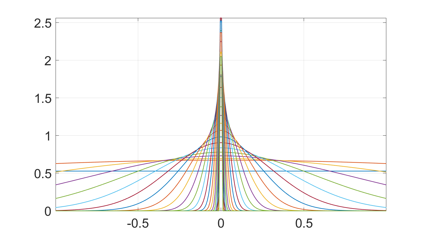
In Fig. 4.1, we illustrate the CP approximation of the collocation tensor on the example of the Newton kernel discretized on a 3D Cartesian grid for , presented for example in [30, 26]. In this case, gives a relative error . We plot the canonical vectors for along the -axis. We can see that there are canonical vectors localized around the singularity at the origin as well as slowly decaying ones, which clearly corresponds to the long-range and short-range behavior of the Newton kernel. We remark here that the number of vectors depends logarithmically on the size of 3D Cartesian grid and the parameter controlling the accuracy of sinc-approximation. For increasing grid size the number of vectors with localized support around the singularity at the origin becomes larger. Choosing smaller -parameter also affects the slow logarithmic increase of the number of required canonical vectors for the tensor representation of the given kernel.
This low-rank CP tensor representation of the Newton kernel has been successfully used by two of coauthors in high accuracy electronic structure calculations [31, 26]. In particular, it was applied for tensor based computation of the Hartree potential (3D convolution of the electron density with the Newton kernel), the nuclear potential operators, and the two-electron integrals tensor, see [26] and references therein. All computations have been performed using huge 3D Cartesian grids with of the order of , providing accuracy close to the results from the analytically based quantum chemical program packages.
4.1.2 Why the Chebyshev polynomial interpolation fails to approximate without range-separation
In this subsection, we consider the ChebTuck approximation Algorithm 4 applied to the CP tensor of the singular Newton kernel and discuss why it may fail to give satisfactory results, which necessitates the use of the range-separated (RS) tensor format [4].
First, we compute the ChebTuck approximation relative error of the CP tensor at the middle slice for different grid size and Chebyshev degree , i.e.,
| (4.5) |
as shown in Table 4.1. We can see that in this case, only when the ChebTuck approximation can give satisfactory results, which is not practical and does not reduce the storage cost.
| 129 | 257 | 513 | 1025 | 2049 | 4097 | 8193 | 16385 | |
|---|---|---|---|---|---|---|---|---|
| 256 | 0.41 | 0.07 | ||||||
| 512 | 0.71 | 0.41 | 0.07 | |||||
| 1024 | 0.92 | 0.71 | 0.41 | 0.07 | ||||
| 2048 | 1.06 | 0.92 | 0.71 | 0.41 | 0.07 | |||
| 4096 | 1.16 | 1.06 | 0.92 | 0.71 | 0.41 | 0.07 |
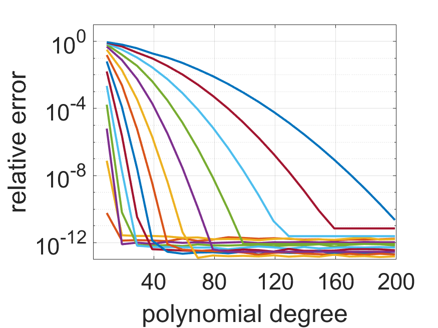
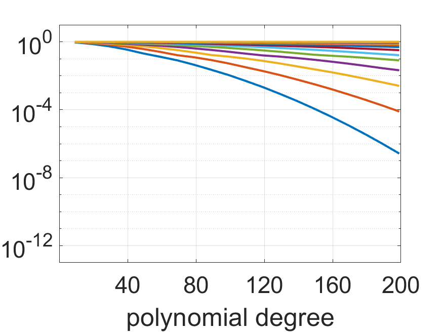
To have a closer look at the behavior, we take the collocation tensor of a single Newton kernel with grid size as an example. In this case, we get a rank CP approximation with relative error . We compute univariate Chebyshev interpolants of all canonical vectors as described in Section 3.2.2 of degree , denoted by . For each canonical vector , we measure the Chebyshev approximation error at the uniform grid points, i.e.,
| (4.6) |
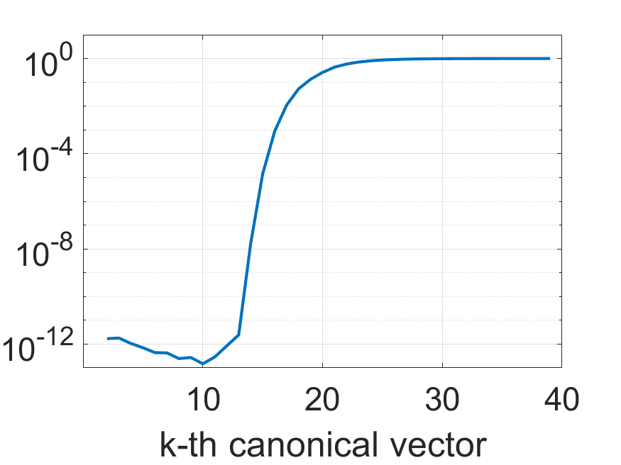
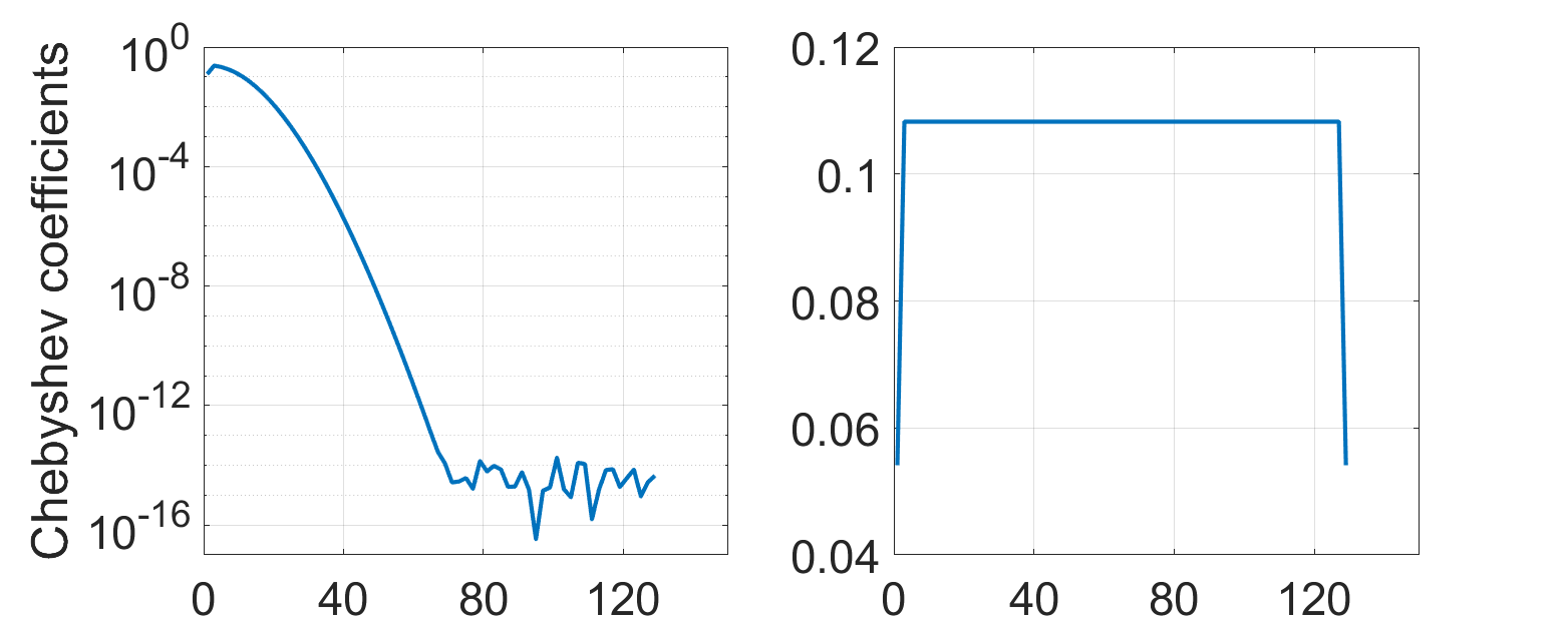
for different Chebyshev degree . The results are shown in Fig. 4.2. We can see that canonical vectors representing the long-range behavior of the Newton kernel, i.e., can be well approximated by low-degree Chebyshev interpolants (left), while for short-range canonical vectors, the convergence is much slower (middle). This is somewhat expected since the short-range canonical vectors have singularities at the origin and require high-degree polynomials to capture the behavior. In Fig. 4.2 right, we plot the Chebyshev approximation error of different canonical vectors for a fixed Chebyshev degree. We can see given this fixed degree , the error of the short-range functions is much larger than the long-range functions with a jump around . The same behavior can also be seen from Fig. 4.3, in which the absolute values of the Chebyshev coefficients of the interpolant of a long-range vector and a short-range vector are shown. We can see that for the long-range vector, the Chebyshev coefficients decay exponentially while for the short-range vector, the coefficients do not decay very much.
This motivates us to perform range-separation of the CP tensor and use the range-separated tensor format [4] first before applying the ChebTuck approximation, which will be discussed in the next subsection.
4.1.3 Range-separation of the CP tensor
For given an appropriately chosen range-separation parameter (see [4] for details of the strategies for choosing ), we further use the range-separated representation of the CP tensor constructed in [4] in the form,
| (4.7) |
where
| (4.8) |
Here Eq. 4.8 represents the sums over the sets of indexes for the long- and short-range canonical vectors in the range-separation splitting of the Newton kernel. Then the short-range part is a highly localized tensor which has very small support and can thus be stored sparsely (see [4] for details), while the ChebTuck approximation can be gainfully applied to the long-range part .
We apply Algorithm 4 to the long-range part and measure the errors of the approximation at the middle slice as in Eq. 4.5 for different grid size and Chebyshev degree , which are shown in Table 4.2. As opposed to the Table 4.1, we can see that the ChebTuck approximation of the long-range part can give satisfactory results already for reasonable Chebyshev degrees . We also show the optimal Tucker ranks, i.e., size of the core tensor of the ChebTuck approximation of the long-range part computed by RHOSVD with relative error for different grid size and Chebyshev degree in Table 4.3. For fixed Chebyshev degree, the Tucker rank of the long-range part only increases logarithmically with the grid size . This indicates that the long-range part can be well approximated by a ChebTuck format with a small number of parameters.
| 129 | 257 | 513 | 1025 | 2049 | 4097 | |
|---|---|---|---|---|---|---|
| 256 | ||||||
| 512 | ||||||
| 1024 | ||||||
| 2048 | ||||||
| 4096 |
| 129 | 257 | 513 | 1025 | 2049 | 4097 | |
|---|---|---|---|---|---|---|
| 256 | 9 | 9 | 9 | 9 | 9 | 9 |
| 512 | 11 | 11 | 11 | 11 | 11 | 11 |
| 1024 | 12 | 12 | 12 | 12 | 12 | 12 |
| 2048 | 13 | 13 | 13 | 13 | 13 | 13 |
| 4096 | 15 | 15 | 15 | 15 | 15 | 15 |
4.2 ChebTuck approximation for multi-particle potentials
In this section, we first recall the construction of the range-separated tensor format [4] for the total potential Eq. 4.1 in a -particle system. Then we consider two practical examples, a bio-molecular system and a lattice-structured compound with vacancies, where we apply the ChebTuck approximation to the long-range part of the total potential.
The total potential of a -particle system in Eq. 4.1 is nothing but a weighted sum of shifted Newton kernels. It was proven in [25] that the tensor representation of the colocation tensor of the total potential can also be obtained by shifting the colocation tensor of the Newton kernel but with a more involved tweak. In fact, it can be obtained with help of shifting and windowing operator applied to the reference potential in Eq. 4.4, see [25],
which applies to every particle located at in an -particle system. Numerically it is obtained by construction of the single generating (reference) potential in a twice larger computational box and shifting it according to coordinates of every particle with further restricting (windowing) it to the original computational domain. Then the total multi-particle potential in Eq. 4.1 is computed as a projected weighted sum of shifted and windowed potentials (see also [26] for more details),
| (4.9) |
It was proven in [4] that tensor representation of type (4.9) in case of a multi-particle system of general type, has almost irreducible large rank, . To overcome this drawback, in [4] a new RS tensor format was introduced based on separation of the long- and short-range skeleton vectors in the generating tensor similar to the single Newton kernel version as in Section 4.1.3 which leads to separable representation for the total sum of potentials,
Thanks to the RS tensor format, the CP-rank of the part of the sum, , containing only the long range components of the canonical vectors of the shifted kernels, scales as , i.e., logarithmically in the number of particles in a molecular system [4]. Such rank compression of the long range part is achieved by applying the RHOSVD method for the canonical to Tucker (C2T) transform, and the subsequent Tucker to canonical (T2C) decomposition [31, 28]. This yields the resulting canonical tensor , with the reduced rank .
One can aggregate the sum of short range tensors (having local supports which do not overlap each other) into the so called “cumulated canonical tensors”, , parametrized only by the coordinates of particle centers and parameters of the localized reference tensor, . Above considerations resulted in the following definition (see [4] for more details).
Definition 4.1.
(RS-canonical tensors [4]). Given a reference tensor supported by a small box such that , the separation parameter , and a set of distinct points , , the RS-canonical tensor format specifies the class of -tensors , which can be represented as a sum of a rank- canonical tensor
| (4.10) |
and a cumulated canonical tensor
| (4.11) |
generated by replication of the reference tensor to the points . Then the RS canonical tensor is represented in the form
| (4.12) |
where in the index size.
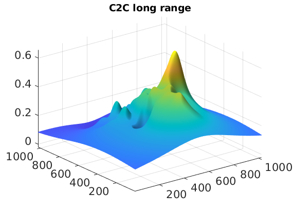
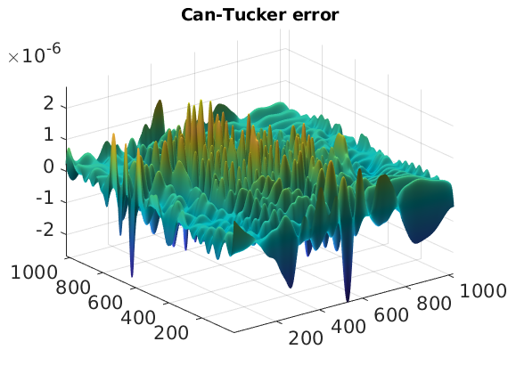
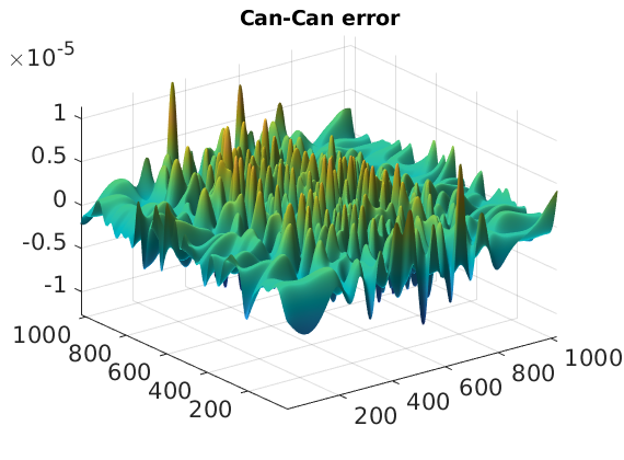
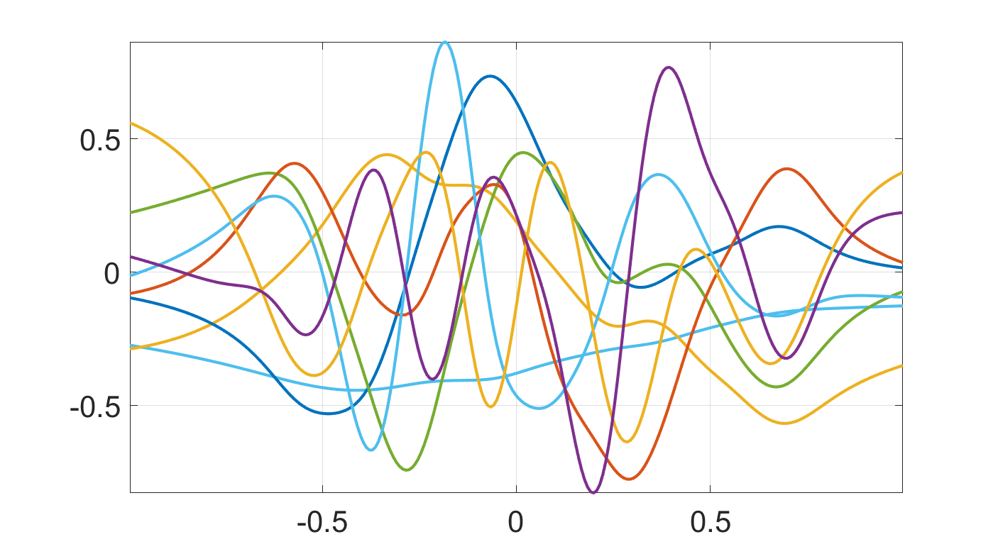
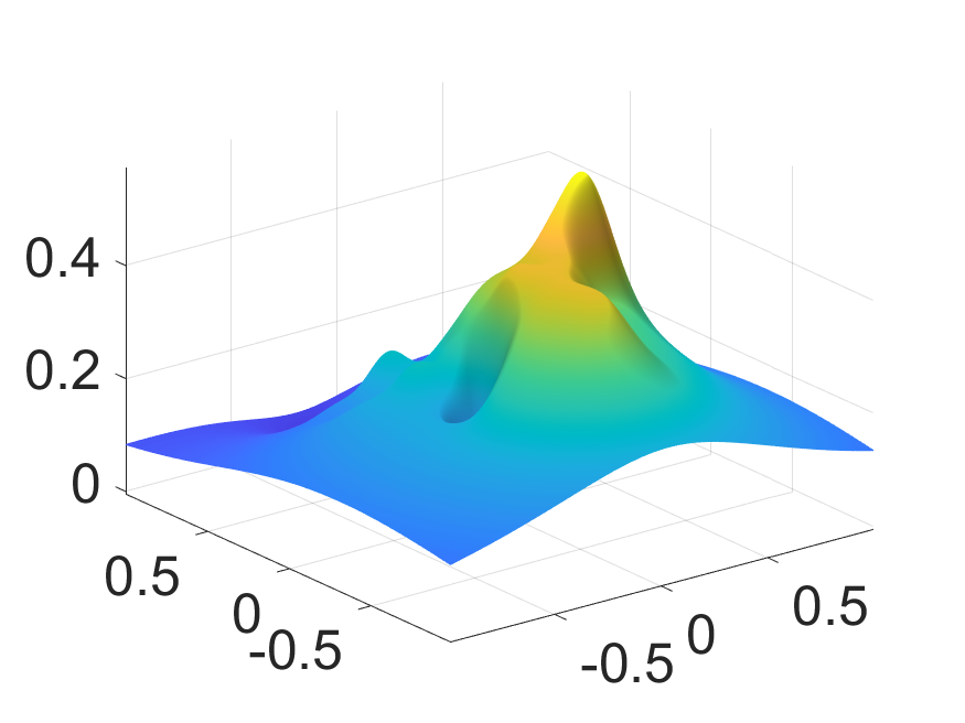
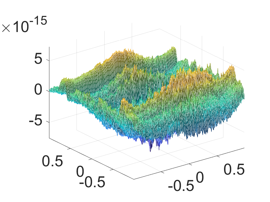
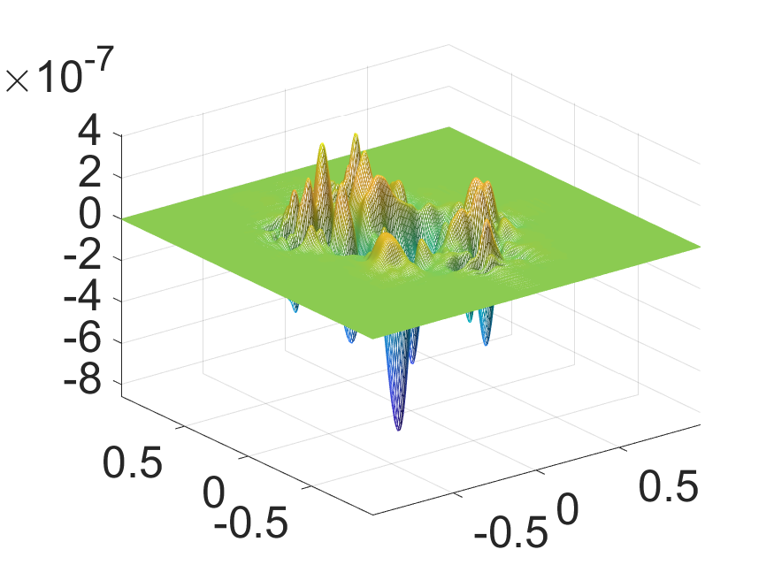
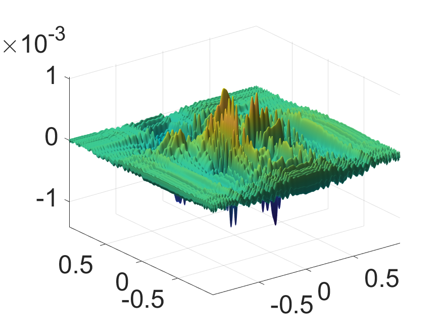
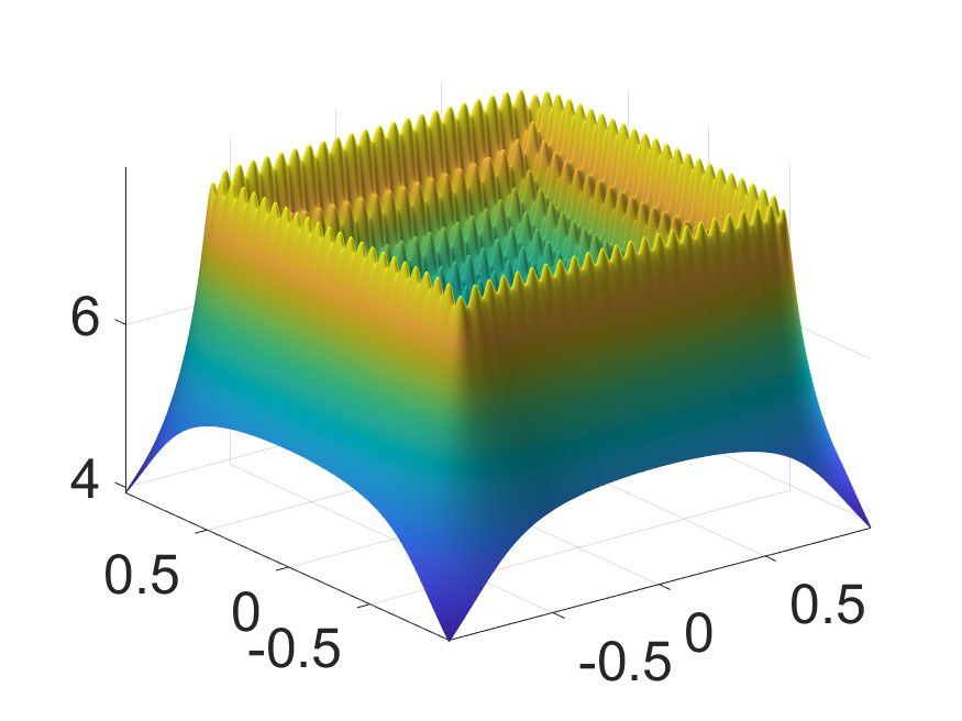
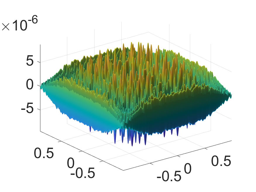
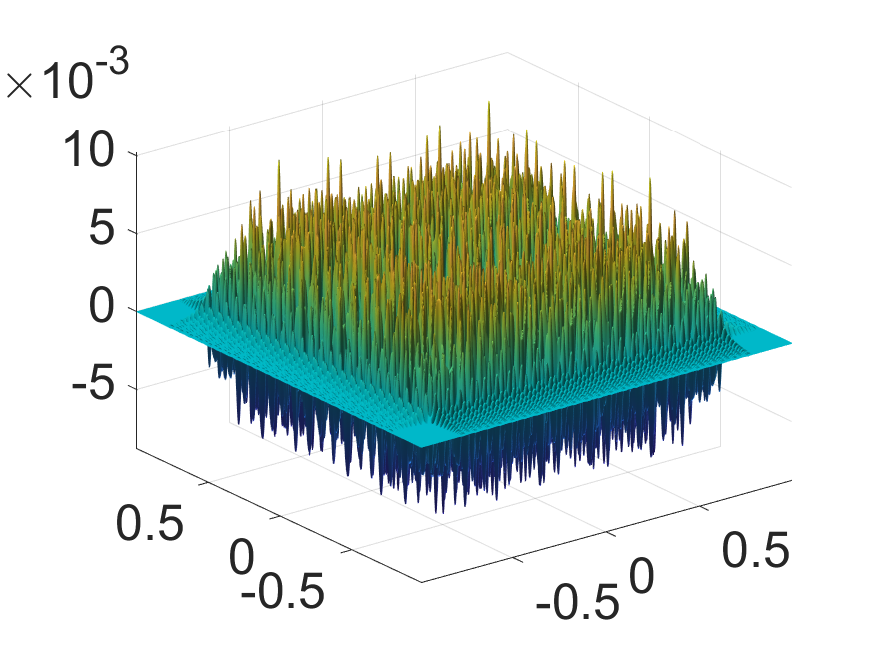
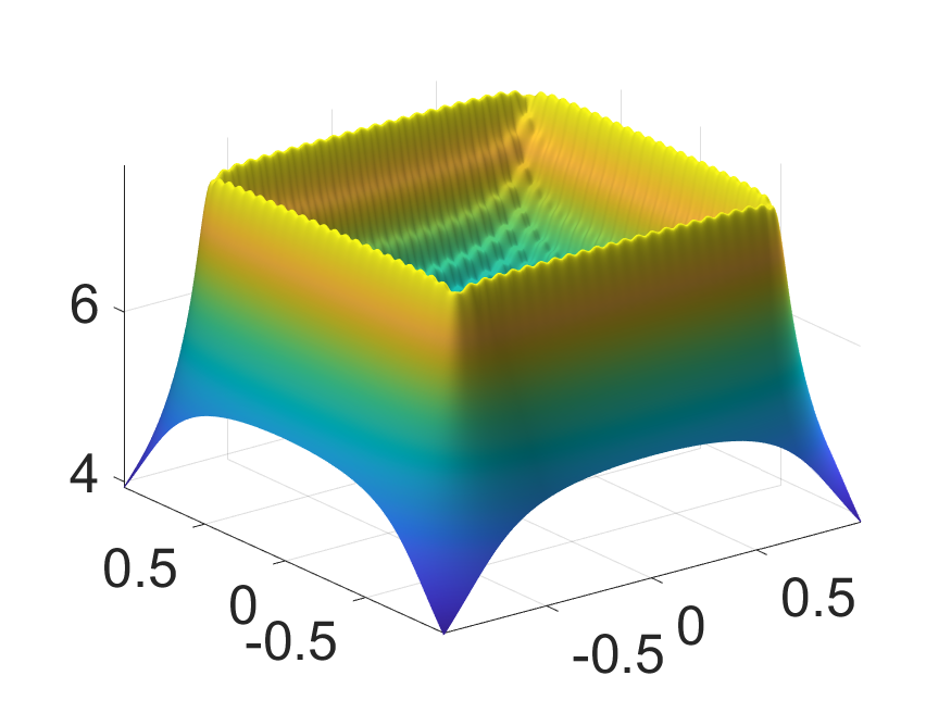
In Fig. 4.4 we visualize the middle slice for the long-range part of the RS tensor, see the left figure, representing the total electrostatic potential of a biomolecule with particles, i.e., of the -particle potential in CP tensor format, with the reduced canonical rank from the original canonical rank computed by RHOSVD-based rank reduction method [31]. We also show the error of the canonical-to-Tucker transform and of the consequent Tucker-to-canonical transform, ultimately canonical-to-canonical transform, in the middle and right figures in Fig. 4.4, respectively. We observe a good approximation error recovering the accuracy of rank truncation in tensor transforms. In Fig. 4.5, we also visualize the several canonical vectors , in the -direction of the long-range part of the same potential as in Fig. 4.4.
In the next sections, we demonstrate the similar accuracy control for the proposed mesh-free two-level tensor approximation applied to the sums of Newton kernels in the case of biomolecules as well as for the lattice type compounds.
4.2.1 A bio-molecule potential with particles
In this section, we consider the ChebTuck approximation to the long range part of a bio-molecule with particles. In this case, the underlining function we want to approximate is given by a 3-dimensional canonical tensor , which can be pre-computed for any given grid size as described in Section 4.2. In this case, Algorithm 1 is not applicable but Algorithms 2, 3 and 4 can be used.
We first consider the runtime and accuracy of Algorithms 2, 3 and 4 for different discretization grid sizes . We set the Chebyshev degrees in each dimension to be and the Tucker-ALS (RHOSVD in case of Algorithm 4) truncation tolerance to be . We record the runtime and error at the middle slice for each case in Tables 4.4 and 4.5. Note that since the trivariate cubic spline in Algorithm 2 is cubic in each spatial direction and for each Chebyshev degree (see Proposition 3.11), we only compute the results for . We observe that the accuracy of the three algorithms is similar. In particular, the Chebyshev interpolants produced by Algorithms 3 and 4 are mathematically equivalent before the Tucker compression, see also Remark 3.3. However, Algorithm 4 is the most efficient which leverages the CP tensor structure of the long-range part as well as the RHOSVD method for Tucker compression. This is consistent with the theoretical estimates in Proposition 3.11. The ChebTuck format also becomes more accurate with increasing grid size which provides more information for the underlying function to be approximated.
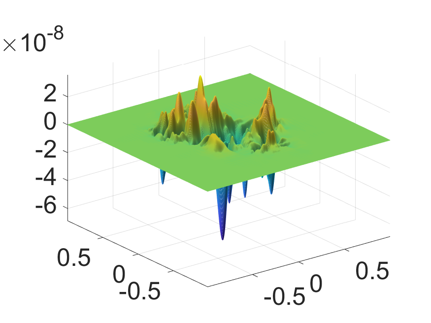
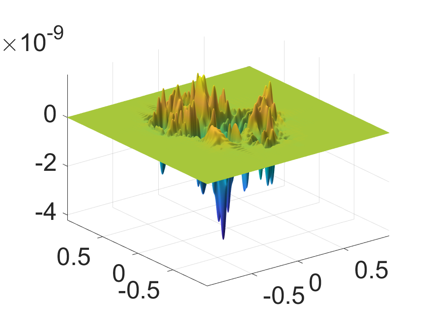
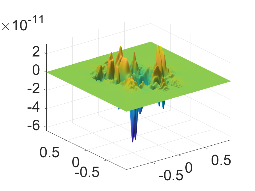
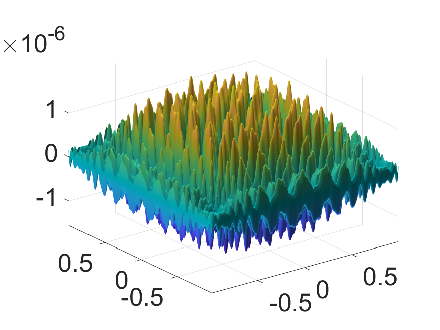
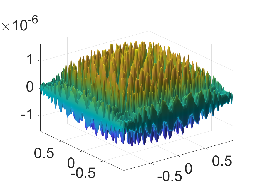
Next, we visualize the ChebTuck approximation error as well as the RHOSVD compression error for the potential with as in Fig. 4.6. In the left figure, we show the middle slice of the approximated potential . Note that here we abuse the notation and use to denote the matrix containing function values of at the uniform grid points in the middle slice, i.e., . In the middle and right figures, we show the error during RHOSVD compressing and the total ChebTuck approximation error, i.e., and , respectively. Note the difference between and as described in Section 3.1. We observe good approximation accuracy of our ChebTuck format. Another notable observation is that the error during RHOSVD compression is much smaller than the prescribed tolerance , which indicates that the singular values decay extremely fast after the first few significant ones. Similar figures are also obtained for larger grid sizes as shown in Fig. 4.7. Our ChebTuck format achieves even higher accuracy for larger grid sizes, consistent with the results in Table 4.5.
| Algorithm 2 | Algorithm 3 | Algorithm 4 | |
|---|---|---|---|
| 13.52 | 0.57 | 0.14 | |
| 0.48 | 0.20 | ||
| 0.50 | 0.28 | ||
| 0.55 | 0.25 |
| Algorithm 2 | Algorithm 3 | Algorithm 4 | |
|---|---|---|---|
We also remark here that the choice of the univariate interpolations in Eq. 3.12 is crucial for the accuracy of the ChebTuck approximation since the convergence rate of the Chebyshev interpolants depends on the smoothness of the univariate interpolations . For example, in Fig. 4.8, we replace the spline interpolation in Eq. 3.12 by piecewise linear (middle) and nearest neighbor (right) interpolation and observe that the ChebTuck format accuracy deteriorates significantly even for a large grid size .
4.2.2 scaling of the Tucker rank of the ChebTuck format
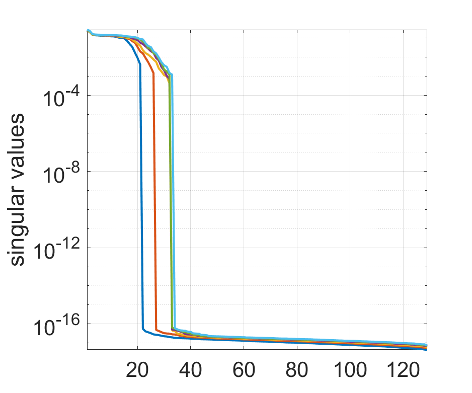
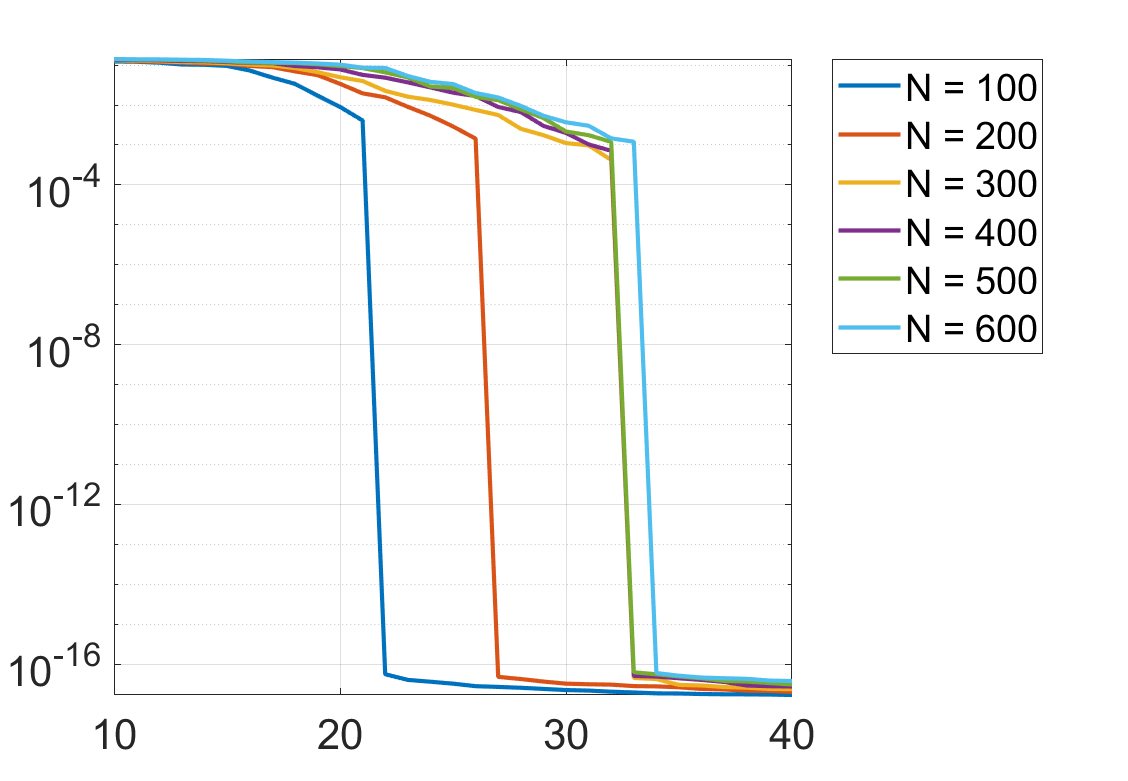
In this section, we demonstrate numerically that the Tucker rank of our mesh-free ChebTuck format of the long-range part of the total potential in a bio-molecular system scales logarithmically with the number of particles , consistent with the result for grid-based range-separated format as in [4, Theorem 3.1]. We consider a bio-molecular system in dimension with particles discretized on Cartesian grid with grid size . For varying particle number and Chebyshev degree , we show the Tucker rank of the ChebTuck format with RHOSVD truncation tolerance in Table 4.6. We can see that the Tucker rank grows only mildly with respect to the number of particles . To have a closer look at the actual behavior, we also plot the singular values of the mode- side matrices of the Chebyshev coefficient tensor (which is in CP format by construction) for in Fig. 4.9. We can see that the singular values drop to the level of machine precision after the first few significant ones, which also explains the behavior of Fig. 4.6, middle figure.
| 9 | 17 | 33 | 65 | 129 | 257 | 513 | 1025 | |
|---|---|---|---|---|---|---|---|---|
| 100 | 9 | 17 | 26 | 26 | 26 | 26 | 26 | 26 |
| 200 | 9 | 17 | 30 | 30 | 30 | 30 | 30 | 30 |
| 300 | 9 | 17 | 31 | 32 | 32 | 32 | 32 | 32 |
| 400 | 9 | 17 | 31 | 32 | 32 | 32 | 32 | 32 |
| 500 | 9 | 17 | 31 | 32 | 32 | 32 | 32 | 32 |
| 600 | 9 | 17 | 31 | 33 | 33 | 33 | 33 | 33 |
4.2.3 A lattice-type compound with vacancies
In this section, we apply our hybrid tensor format ChebTuck to the problem of low-parametric approximation of electrostatic potentials of the large lattice-type structures, see [25]. In this case, the charge centers in Eq. 4.1 are located on a regular grid. For a lattice-type structure of size with particles, the canonical representation of its potential is given by a CP tensor of size with and rank .
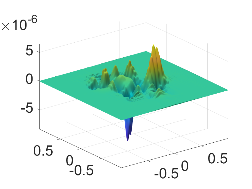
We apply Algorithm 4 to approximate the potential with Chebyshev degrees and Tucker-ALS truncation tolerance . The results are shown in Fig. 4.10. We observe that the error of our method is of the magnitude , which is not as good as the bio-molecule example since we have not separated the long-range and short-range parts. On the other hand, see Fig. 4.11, if we separate the long-range part of the potential by taking out the last canonical vectors, the error is reduced to the magnitude , which is consistent with the prescribed tolerance and previous results on the bio-molecule example.
The numerical results confirm the efficiency of the new mesh-less hybrid tensor decomposition on the example of complicated multi-particle potential arising in quantum chemistry, bio-molecular modeling, etc. Indeed, it demonstrates the same approximation error as for the established grid-based tensor approximation method applied on relatively large grids, required for the good resolution of the complicated multi-particle potentials.
5 Conclusions
We introduce and analyze a mesh-free two-level hybrid Tucker tensor format for approximation of multivariate functions in with both high and reduced regularity, which combines the tensor product Chebyshev polynomial interpolation in the global computational domain with the ALS-based Tucker decomposition of the Chebyshev coefficient tensor.
For functions with multiple cusps (or even stronger singularities) our method applies to the long-range component of the target function represented in low-rank RS tensor format. In case of orthogonal set of interpolating functions like Chebyshev polynomials, the subsequent rank optimization via ALS-type rank-structured decomposition of the coefficient tensor leads to nearly optimal -rank Tucker decomposition of the initial function with merely the same rank parameter as for the alternative grid-based Tucker-ALS approximation.
We present numerous numerical tests demonstrating the efficiency of the proposed techniques on the examples of many-particle electrostatic potentials in bio-molecular systems and in lattice-structured compounds. In particular, we observe from numerical examples the following beneficial features of our method.
-
•
Fast mesh-free Tucker decomposition with quasi-optimal rank parameter in application to rather regular functions.
-
•
Efficient mesh-free Tucker tensor decomposition of the long-range part for the multi-particle electrostatic potentials in , composed of the large sum of singular Newton kernels.
-
•
The new mesh-free two-level hybrid Tucker tensor format demonstrates the efficiency in application to lattice-structured compounds with monopoles and dipoles like structures.
-
•
In case of input function presented in the canonical (CP) tensor format our method needs only a small number of 1D-Chebyshev interpolations of the 1D-canonical skeleton vectors.
Finally, we notice that the presented techniques can be applied to the Green functions for various elliptic operators and can be extended to higher dimensions. In the latter case, the combination with the TT, QTT or H-Tucker tensor decompositions is necessary to avoid the curse of dimensionality.
References
- [1] M. Bachmayr, R. Schneider, and A. Uschmajew, Tensor networks and hierarchical tensors for the solution of high-dimensional partial differential equations, Foundations of Computational Mathematics, 16 (2016), pp. 1423–1472.
- [2] M. Bebendorf, Adaptive cross approximation of multivariate functions, Constructive Approximation, 34 (2011), pp. 149–179.
- [3] P. Benner and H. Faßbender, Modellreduktion: Eine systemtheoretisch orientierte Einführung, Springer Verlag, Berlin, 2024.
- [4] P. Benner, V. Khoromskaia, and B. N. Khoromskij, Range-separated tensor format for many-particle modeling, SIAM Journal on Scientific Computing, 40 (2018), pp. A1034–A1062.
- [5] P. Benner, V. Khoromskaia, B. N. Khoromskij, and M. Stein, Fast tensor-based electrostatic energy calculations for protein-ligand docking problem, manuscript, (2024).
- [6] P. Benner, V. L. Mehrmann, and D. C. Sorensen, Dimension reduction of large-scale systems, Springer Verlag, 2005.
- [7] J.-P. Berrut, Rational functions for guaranteed and experimentally well-conditioned global interpolation, Computers & Mathematics with Applications, 15 (1988), pp. 1–16.
- [8] J.-P. Berrut and L. N. Trefethen, Barycentric Lagrange interpolation, SIAM Review, 46 (2004), pp. 501–517.
- [9] C. Bertoglio and B. N. Khoromskij, Low-rank quadrature-based tensor approximation of the galerkin projected Newton/Yukawa kernels, Computer Physics Communications, 183 (2012), pp. 904–912.
- [10] D. Braess, Nonlinear approximation theory, Springer-Verlag, Berlin, 1986.
- [11] M. Che and Y. Wei, Randomized algorithms for the approximations of Tucker and the tensor train decompositions, Advances in Computational Mathematics, 45 (2019), pp. 395–428.
- [12] P. L. Chebyshev, Sur les questions de minima qui se rattachent á la representation approximative des fonctions, Mem. Acad. Sci. Pétersb., 7 (1859).
- [13] C. De Boor, A practical guide to splines, Springer New York, 1978.
- [14] L. De Lathauwer, B. De Moor, and J. Vandewalle, A multilinear singular value decomposition, SIAM Journal on Matrix Analysis and Applications, 21 (2000), pp. 1253–1278.
- [15] , On the best Rank-1 and Rank- approximation of higher-order tensors, SIAM Journal on Matrix Analysis and Applications, 21 (2000), pp. 1324–1342.
- [16] S. Dolgov, D. Kressner, and C. Stroessner, Functional Tucker approximation using Chebyshev interpolation, SIAM Journal on Scientific Computing, 43 (2021), pp. A2190–A2210.
- [17] T. A. Driscoll, N. Hale, and L. N. Trefethen, Chebfun guide, 2014.
- [18] Z. Gao, J. Liang, and Z. Xu, A kernel-independent sum-of-exponentials method, Journal of Scientific Computing, 93 (2022), p. 40.
- [19] L. Greengard, S. Jiang, and Y. Zhang, The anisotropic truncated kernel method for convolution with free-space Green’s functions, SIAM Journal on Scientific Computing, 40 (2018), p. A3733–A3754.
- [20] W. Hackbusch and B. N. Khoromskij, Towards H-matrix approximation of linear complexity, In: Operator Theory: Advances and Applications, 121 (2001), pp. 194–220.
- [21] W. Hackbusch and B. N. Khoromskij, Low-rank Kronecker-product approximation to multi-dimensional nonlocal operators. part I. separable approximation of multi-variate functions, Computing, 76 (2006), pp. 177–202.
- [22] B. Hashemi and L. N. Trefethen, Chebfun in three dimensions, SIAM Journal on Scientific Computing, 39 (2017), pp. C341–C363.
- [23] F. L. Hitchcock, The expression of a tensor or a polyadic as a sum of products, Journal of Mathematics and Physics, 6 (1927), pp. 164–189.
- [24] V. Kazeev, O. Reichmann, and C. Schwab, Low-rank tensor structure of linear diffusion operators in the TT and QTT formats, Linear Algebra and its Applications, 438 (2013), pp. 4204–4221.
- [25] V. Khoromskaia and B. N. Khoromskij, Grid-based lattice summation of electrostatic potentials by assembled rank-structured tensor approximation, Computer Physics Communications, 185 (2014), pp. 3162–3174.
- [26] V. Khoromskaia and B. N. Khoromskij, Tensor numerical methods in quantum chemistry, De Gruyter, Berlin, 2018.
- [27] V. Khoromskaia and B. N. Khoromskij, Ubiquitous nature of the reduced higher order SVD in tensor-based scientific computing, Frontiers in Applied Mathematics and Statistics, 8:826988 (2022).
- [28] B. Khoromskij and V. Khoromskaia, Low rank Tucker-type tensor approximation to classical potentials, Open Mathematics, 5 (2007), pp. 523–550.
- [29] B. N. Khoromskij, -Quantics approximation of N-d tensors in high-dimensional numerical modeling, Constructive Approximation, 34 (2011), pp. 257–289.
- [30] B. N. Khoromskij, Tensor numerical methods in scientific computing, De Gruyter, Berlin, 2018.
- [31] B. N. Khoromskij and V. Khoromskaia, Multigrid accelerated tensor approximation of function related multidimensional arrays, SIAM Journal on Scientific Computing, 31 (2009), pp. 3002–3026.
- [32] D. Kressner, B. Vandereycken, and R. Voorhaar, Streaming tensor train approximation, SIAM Journal on Scientific Computing, 45 (2023), pp. A2610–A2631.
- [33] C.-C. Lin, P. Motamarri, and V. Gavini, Tensor-structured algorithm for reduced-order scaling large-scale Kohn-Sham density functional theory calculations, npj Computational Materials, 7 (2021), p. 50.
- [34] L. Ma and E. Solomonik, Fast and accurate randomized algorithms for low-rank tensor decompositions, Advances in neural information processing systems, 34 (2021), pp. 24299–24312.
- [35] C. Marcati, M. Rakhuba, and C. Schwab, Tensor rank bounds for point singularities in , Advances in Computational Mathematics, 48, 18 (2022).
- [36] J. C. Mason, Near-best multivariate approximation by Fourier series, Chebyshev series and Chebyshev interpolation, Journal of Approximation Theory, 28 (1980), pp. 349–358.
- [37] J. C. Mason, Minimal projections and near-best approximations by multivariate polynomial expansion and interpolation, in Multivariate Approximation Theory II: Proceedings of the Conference held at the Mathematical Research Institute at Oberwolfach, Black Forest, February 8–12, 1982, Springer, 1982, pp. 241–254.
- [38] J. C. Mason and D. C. Handscomb, Chebyshev polynomials, Chapman and Hall/CRC, 2002.
- [39] I. V. Oseledets, Tensor-train decomposition., SIAM Journal on Scientific Computing, 33 (2011), pp. 2295–2317.
- [40] I. V. Oseledets, D. Savostianov, and E. E. Tyrtyshnikov, Tucker dimensionality reduction of three-dimensional arrays in linear time, SIAM Journal on Matrix Analysis and Applications, 30 (2008), pp. 939–956.
- [41] M. Rakhuba and I. Oseledets, Calculating vibrational spectra of molecules using tensor train decomposition, The Journal of Chemical Physics, 145, 124101 (2016).
- [42] M. Rakhuba and I. V. Oseledets, Fast multidimensional convolution in low-rank tensor formats via cross approximation, SIAM Journal on Scientific Computing, 37 (2015), pp. A565–A582.
- [43] L. Risthaus and M. Schneider, Solving phase-field models in the tensor train format to generate microstructures of bicontinuous composites, Applied Numerical Mathematics, 178 (2022), pp. 262–279.
- [44] A. K. Saibaba, R. Minster, and M. Kilmer, Efficient randomized tensor-based algorithms for function approximation and low-rank kernel interactions, Advances in Computational Mathematics, 48 (2022), p. 66.
- [45] F. Stenger, Numerical methods based on Sinc and analytic functions, Springer-Verlag, 1993.
- [46] C. Strössner, B. Sun, and D. Kressner, Approximation in the extended functional tensor train format, Advances in Computational Mathematics, 50, 54 (2024).
- [47] V. Subramanian, S. Das, and V. Gavini, Tucker tensor approach for accelerating Fock Exchange computations in a real-space finite-element discretization of generalized Kohn-Sham density functional theory, Journal of Chemical Theory and Computation, 20 (2024), pp. 3566–3579.
- [48] L. N. Trefethen, Approximation theory and approximation practice, extended edition, SIAM, 2019.
- [49] L. R. Tucker, Some mathematical notes on three-mode factor analysis, Psychometrika, 31 (1966), pp. 279–311.
- [50] H. Yserentant, An iterative method for the solution of Lplace-like equations in high and very high space dimensions, Numerische Mathematik, 156 (2024), pp. 777–811.