Correlated study on some $B_{c}\rightarrow\text{ }P$ and $B_{c}\rightarrow\text{ }S$ wave channels in light of new inputs

Abstract

This study investigates the decay modes of the $B_{c}$ meson, focusing on semileptonic and nonleptonic decay into S and P wave charmonia. The primary objective is to extract the shape parameter of the $B_{c}$ meson distribution amplitude through a data-driven approach, utilizing the lattice results on $B_{c}\rightarrow\eta_{c},J/\psi$ semileptonic form factors and yielding an estimate of ${\omega_{B}}_{c}=0.998(34)$ for the same. We use the form factors derived from the modified perturbative QCD framework in the analysis. This result and various other inputs on the radiative decays of the P wave charmonia enable us to estimate the $q^{2}$ shapes of the $B_{c}\rightarrow\chi_{c0},\chi_{c1}$ and $h_{c}$ form factors using pole expansion parametrization. Using these results, we have obtained predictions of LFUV observables $R(\chi_{c0})=0.169(11)$, $R(\chi_{c1})=0.126(2)$ and $R(h_{c})=0.113(3)$. Finally, we have presented predictions for branching ratios of some nonleptonic decay modes of the $B_{c}$ meson into S and P wave charmonia in the same modified perturbative QCD framework.

1 Introduction

The $B_{c}$-meson is a heavy quarkonium with mixed-heavy flavours, which could be useful for studying heavy-quark dynamics. At the same time, it is stable against strong and electromagnetic interactions as it lies below the $B\bar{D}$ threshold and can only decay through weak interactions. It is an ideal system for studying weak decays of both the heavy quarks. This possibility offers a promising opportunity to study various nonleptonic and semileptonic weak decays of heavy mesons. Similar to $B\to D^{(*)}\ell^{-}\bar{\nu}$ (with $\ell=e,\mu,\tau$) decays the semileptonic decays of $B_{c}$ meson to the $S$ and $P$-wave charmoniums will be useful to extract the Cabibbo-Kobayashi-Maskawa (CKM) matrix element $|V_{cb}|$ and in the indirect search of the new interactions beyond the standard model (BSM). The modes with light leptons are less sensitive to BSM physics and, hence, could be used to extract $|V_{cb}|$ while the mode with $\ell=\tau$ is expected to help probe BSM scenarios. We define observables like the ratios of the decay rates

$$R(P(V))=\frac{\Gamma(B_{c}^{-}\to P(V)\tau^{-}\bar{\nu})}{\Gamma(B_{c}^{-}\to P(V)\mu^{-}\bar{\nu})}.$$ (1)

These observables are expected to be potentially sensitive to BSM interactions. At the present level of accuracy, we have observed deviations in the measured values of $R(D^{(*)})$ as compared to the respective SM predictions hflavnew ; HFLAV:2022esi ; Ray:2023xjn . The measurement of the observables in the $B_{c}$ decays will be important to gain complementary phenomenological information. Such studies can help improve our understanding of the nature of the anomalous results seen in B-meson decays. Moreover, any BSM physics altering these modes’ results should be affected and constrained by other $b\to c$ transitions.

The LHCb and CMS collaborations have measured this ratio in $B_{c}^{-}\to J/\psi\ell^{-}\bar{\nu}$ decays which are given as folllows LHCb:2017vlu :

$$R(J/\psi)=\frac{\Gamma(B_{c}^{-}\to J/\psi\tau^{-}\bar{\nu})}{\Gamma(B_{c}^{-}\to J/\psi\mu^{-}\bar{\nu})}=0.71\pm 0.17(stat)\pm 0.18(syst)~~~~~\text{(LHCb),}$$ (2)

$$R(J/\psi)=0.17^{+0.18}_{-0.17}(stat.)^{+0.21}_{-0.22}(syst.)^{+0.19}_{-0.18}(theo)=0.17\pm 0.33~~~\text{( CMS)}.$$ (3)

Both the measured values have significant errors and are marginally consistent with each other at their 1$\sigma$ uncertainties. We must wait for more precise data to look for possible new physics (NP) effects. However, precise predictions of all the related observables in the SM are equally important. A model-independent approach regarding the form factors Cohen:2019zev leads to the SM prediction of $0.25(3)$. The HPQCD lattice collaboration has recently extracted the $B_{c}\to J/\psi$ form-factors over the full kinematically allowed region Harrison:2020gvo . They have predicted $R(J/\psi)=0.2582(38)$ Harrison:2020nrv , which is so far the most precise prediction and in tension with the LHCb result given above but in agreement with the measured value at the CMS. So far, no inputs on the form factors of other $B_{c}\to S$ or $B_{c}\to P$ wave charmoniums from the lattice are available. Neither data on the corresponding semileptonic or non-leptonic rates is available. Several QCD models exist in the literature, and based on the modelling of the form factors, the value of $R(J/\psi)$ lies in the range $[0,0.48]$ Anisimov:1998uk ; Kiselev:2002vz ; Ivanov:2006ni ; Hernandez:2006gt ; Wang:2012lrc ; Rui:2017pre ; Rui:2018kqr ; PhysRevD.97.113001 ; Hu:2019bdf .

The form factors in $B_{c}\to J/\psi$, $B_{c}\to\eta_{c}$, $B_{c}\to\chi_{c0}$, $B_{c}\to\chi_{c1}$ and $B_{c}\to h_{c}$ transitions have been calculated in the perturbative QCD (PQCD) framework Wang:2012lrc ; Rui:2017pre ; Rui:2018kqr ; PhysRevD.97.113001 ; Hu:2019bdf . Apart from the perturbatively calculable hard functions, these form factors depend on the non-perturbative wave functions of $B_{c}$ and other mesons involved in the respective processes. Therefore, estimates of the relevant wave functions should be made to obtain the form factors in the respective decays. In this analysis, we constrain these wave functions using the lattice inputs on $B_{c}\to J/\psi$ form factors Harrison:2020gvo and the available data on the respective radiative decays of the corresponding charmonium states. In addition, we have used the inputs on $B_{c}\to\eta_{c}$ form factors, which we have extracted using the available information on $B_{c}\to J/\psi$ form factors from the lattice in combination with the heavy-quark-spin-symmetry (HQSS), the method is similar to the one used in ref. Biswas:2023bqz . In the earlier perturbative QCD analyses Wang:2012lrc ; Rui:2017pre ; Rui:2018kqr ; PhysRevD.97.113001 ; Hu:2019bdf , model-dependent inputs were used to obtain the respective wave functions.

To obtain the semileptonic rates, we need to know the shape of the respective form factors in the kinematically allowed $q^{2}$ (lepton invariant mass squared) regions. However, calculating the form factors in the PQCD approach is reliable only in the large recoil regions. We obtain the $q^{2}$ shape of the form factors in $B_{c}\to\eta_{c}\ell^{-}\bar{\nu}$ decays using the HQSS symmetry. After predicting the PQCD form factors at $q^{2}=0$, the shape of the form factors in $B_{c}\to\chi_{c0}\ell\nu$, $B_{c}\to\chi_{c1}\ell\nu$ and $B_{c}\to h_{c}\ell\nu$ decays are obtained by using the pole expansion technique which we will discuss later. Finally, using these form factors, we have predicted the $q^{2}$ distribution of the respective rates, the branching fractions, and the ratios $R(\eta_{c})$, $R(\chi_{c0})$, $R(\chi_{c1})$ and $R(h_{c})$. In addition, we have predicted a couple of angular observables in the SM. We take this opportunity to predict the branching fractions of a couple of non-leptonic decay modes of $B_{c}$ meson to charmonium and a light meson.

The paper is structured as follows: In section 2 we describe the analytic expressions of the various physical observables that we intend to predict in this work and briefly discuss about the respective form factors in modified pQCD framework and light cone distribution amplitudes(LCDAs) of the participating mesons. In section 3 we extract the $B_{c}$, $J/\psi$ and $\eta_{c}$ LCDA shape parameters and present our predictions of the corresponding form factors at $q^{2}=0$. In section 4 we obtain information of $B_{c}\rightarrow P$ semileptonic form factors over full physical $q^{2}$ region utilizing suitable extrapolation technique and present predictions of some physical observables. In section 5 we present our predictions of branching ratios of a number of nonleptonic decay of $B_{c}$ meson into $S$ and $P$ wave charmonia. Finally in section 6 we briefly summarize our work.

2 Theoretical background for $B_{c}\rightarrow$ charmonium semileptonic modes

In this section, we will focus primarily on the theoretical aspects of our work. We present the theory expressions of the different observables related to the semileptonic decays in the SM, which we will predict in this work.

2.1 Physical Observables

In the SM, the effective Hamiltonian for $b\rightarrow c\ell^{-}\bar{\nu}$ decay can be written as

$$\mathcal{H}_{eff}=\frac{G_{F}}{\sqrt{2}}V_{cb}^{*}\bar{b}\gamma_{\mu}(1-\gamma_{5})c\otimes\bar{\nu_{l}}\gamma^{\mu}(1-\gamma_{5})l,$$ (4)

where $G_{F}=1.16637\times 10^{-5}\hskip 2.84526ptGeV^{-2}$ is the Fermi coupling constant, and $V_{cb}$ is one of the CKM matrix elements. Using the above effective Hamiltonian, we have the following differential decay widths Tanaka:2010se ; Tanaka:2012nw ; Hu:2019bdf

$$\begin{split}\frac{d\Gamma(B_{c}\rightarrow Pl^{-}\bar{\nu}_{l})}{dq^{2}}=\frac{G_{F}^{2}|V_{cb}|^{2}}{384\pi^{3}m_{B_{c}}^{3}}\sqrt{\lambda(q^{2})}\left(1-\frac{m_{l}^{2}}{q^{2}}\right)^{2}&\Bigg{[}3m_{l}^{2}(H^{s}_{V,t}(q^{2}))^{2}+(m_{l}^{2}+2q^{2})(H_{V,0}(q^{2}))^{2}\Bigg{]},\end{split}$$ (5)

for the decay to a pseudoscalar meson $P$, like $\eta_{c}$ or $\chi_{c0}$, and

$$\begin{split}\frac{d\Gamma(B_{c}\rightarrow Vl^{-}\bar{\nu}_{l})}{dq^{2}}=\frac{G_{F}^{2}|V_{cb}|^{2}}{384\pi^{3}m_{B_{c}}^{3}}\sqrt{\lambda(q^{2})}\left(1-\frac{m_{l}^{2}}{q^{2}}\right)^{2}&\Bigg{[}(m_{l}^{2}+2q^{2})(H_{V,+}^{2}+H_{V,-}^{2}+H_{V,0}^{2})\\ &+3m_{l}^{2}H_{V,t}^{2}\Bigg{]},\end{split}$$ (6)

for a final state vector meson $V$, like $J/\psi$, $\chi_{c1}$, $h_{c}$ etc. In the above equations, the phase space factor is expressed as

$$\lambda(q^{2})=(m_{B_{c}}^{2}+m_{P/V}^{2}-q^{2})^{2}-4m_{B_{c}}^{2}m_{P/V}^{2},$$ (7)

with $m_{l}$, $m_{P/V}$ are the masses of the respective lepton and the final state meson. The total decay width is obtained by integrating $d\Gamma/dq^{2}$ over the physical $q^{2}$ region, which ranges from $m_{l}^{2}$ to $(m_{B_{c}}-m_{P/V})^{2}$.

In the expressions above the rates are written as a functions of the helicity amplitudes $H_{V,0}^{s},H_{V,t}^{s},H_{V,\pm},$ $H_{V,0},H_{V,t}$, which are related to the QCD form factors as given below:

$$\begin{split}H_{V,0}^{s}(q^{2})&=\sqrt{\frac{\lambda(q^{2})}{q^{2}}}F_{+}(q^{2}),\\ H_{V,t}^{s}(q^{2})&=\frac{m_{B_{c}}^{2}-m_{P}^{2}}{\sqrt{q^{2}}}F_{0}(q^{2}),\\ H_{V,\pm}(q^{2})&=(m_{B_{c}}\pm m_{V})A_{1}(q^{2})\mp\frac{\sqrt{\lambda(q^{2})}}{m_{B_{c}}\pm m_{V}}V(q^{2}),\\ H_{V,0}(q^{2})&=-\frac{m_{B_{c}}\pm m_{V}}{2m_{V}\sqrt{q^{2}}}\left[(m_{B_{c}}^{2}-m_{V}^{2}-q^{2})A_{1}(q^{2})-\frac{\lambda(q^{2})}{(m_{B_{c}}\pm m_{V})^{2}}A_{2}(q^{2})\right],\\ H_{V,t}(q^{2})&=-\sqrt{\frac{\lambda(q^{2})}{q^{2}}}A_{0}(q^{2}),\end{split}$$ (8)

where $(m_{B_{c}}+m_{V})$ and $(m_{B_{c}}-m_{V})$ are for $B_{c}\rightarrow S$ and $B_{c}\rightarrow P$ wave channels respectively. The QCD form factors which are obtained as the transition matrix elements of the charged weak quark current are defined above. Depending on the final state charmonium mesons, the corresponding transition matrix elements can be parametrized in terms of the appropriate form factors. In case the final state meson is a pseudoscalar or scalar meson, the transition matrix element can be parametrized in terms of two form factors $F_{+}$ and $F_{0}$,

$$\begin{split}\left\langle P(p_{2})|\bar{c}\gamma^{\mu}b|B_{c}(p_{1})\right\rangle=&\left[(p_{1}+p_{2})^{\mu}-\frac{m_{B_{c}}^{2}-m_{P}^{2}}{q^{2}}q^{\mu}\right]F_{+}(q^{2})+\frac{m_{B_{c}}^{2}-m_{P}^{2}}{q^{2}}q^{\mu}F_{0}(q^{2}),\end{split}$$ (9)

with $q^{\mu}=p_{1}^{\mu}-p_{2}^{\mu}$. In case the final state meson is a vector or axial-vector meson, the transition matrix elements are parametrized in terms of four form factors $A_{0}$, $A_{1}$, $A_{2}$ and $V$,

$$\left\langle V(p_{2})|\bar{c}\gamma^{\mu}b|B_{c}(p_{1})\right\rangle=\frac{2iV_{0}(q^{2})}{m_{B_{c}}\pm m_{V}}\epsilon^{\mu\nu\rho\sigma}\epsilon_{\nu}^{*}p_{2\rho}p_{1\sigma},$$ (10)

and,

$$\begin{split}\left\langle V(p_{2})|\bar{c}\gamma^{\mu}\gamma_{5}b|B_{c}(p_{1})\right\rangle&=2m_{V}A_{0}(q^{2})\frac{\epsilon^{*}\cdot q}{q^{2}}q^{\mu}+(m_{B_{c}}\pm m_{V})A_{1}(q^{2})\left[\epsilon^{*\mu}-\frac{\epsilon^{*}\cdot q}{q^{2}}q^{\mu}\right]\\ &-A_{2}(q^{2})\frac{\epsilon^{*}\cdot q}{m_{B_{c}}\pm m_{V}}\left[(p_{1}+p_{2})^{\mu}-\frac{m_{B_{c}}^{2}-m_{V}^{2}}{q^{2}}q^{\mu}\right].\end{split}$$ (11)

There are relations among these form factors at maximum recoil, i.e., $q^{2}=0$, are as

$$F_{+}(0)=F_{0}(0),$$ (12)

for form factors defined in Eqn.(9), and for those defined in Eqn.(11),

$$\begin{split}\text{For S wave:}\qquad 2rA_{0}(0)=&(1+r)A_{1}(0)-(1-r)A_{2}(0),\\ \text{For P wave:}\qquad 2rA_{0}(0)=&(1-r)A_{1}(0)-(1+r)A_{2}(0),\end{split}$$ (13)

hold. These form factors are the non-perturbative unknowns. To get the $q^{2}$ distributions of the decay rates, we need to know the $q^{2}$ shapes of these form factors which we will discuss in the next subsection.

Integrating the differential decay rates over the kinematically allowed ranges of $q^{2}$ we will get the total decays rates, hence we will obtain the branching fractions by multiplying these decay rates by the lifetime of the $B_{c}$ meson. In addition to branching ratios, there are three additional observables for the considered $B_{c}$ semileptonic decays, that find significance in probing contributions to physics beyond the standard model. These are the longitudinal polarization of the $\tau$ lepton, $P_{\tau}$, vector and axial-vector meson longitudianl polarization fraction, $F_{L}(V)$, and forward backward asymmetry for lepton modes, $A_{FB}(l)$.

• For the first of the three observables, the tau lepton polarization’s definition depends on the frame considered. We follow the framework considered by the authors in Tanaka:2010se , in which the spatial components of the momentum transfer $q^{\mu}=p_{B_{c}}^{\mu}-p_{P/V}^{\mu}$ vanish, $p_{B_{c}}^{\mu}$ and $p_{M}^{\mu}$ being the four-momenta of the initial state $B_{c}$ and the final state mesons respectively. The coordinate system they have considered is such that the direction of momenta of the initial and the final state mesons are along the z- axis, and that for the $\tau$ lepton it lies in the x-z plane. We consider the definition of $P_{\tau}$ from previous works Tanaka:2010se ; Tanaka:2012nw ; Hu:2019bdf , which has the form

  $$P_{\tau}=\frac{\Gamma_{+}-\Gamma_{-}}{\Gamma_{+}+\Gamma_{-}},$$ (14)

  where $\Gamma_{\pm}$ denotes the decay rate of the decay $B_{c}\rightarrow P(V)\tau\nu_{\tau}$ with the $\tau$ lepton helicity $\pm 1/2$. The explicit expressions of $\Gamma_{\pm}$ has been taken from Sakaki:2013bfa . In our present work, however we will only be focussing on the SM contributions, which has the form

  $$\begin{split}\frac{d\Gamma_{+}}{dq^{2}}=&\frac{G_{F}^{2}|V_{cb}|^{2}}{192\pi^{3}m_{B_{c}}^{3}}q^{2}\sqrt{\lambda(q^{2})}\left(1-\frac{m_{\tau}^{2}}{q^{2}}\right)^{2}\frac{m_{\tau}^{2}}{2q^{2}}(H_{V,0}^{s\text{ }2}+3H_{V,t}^{s\text{ }2}),\\ \frac{d\Gamma_{-}}{dq^{2}}=&\frac{G_{F}^{2}|V_{cb}|^{2}}{192\pi^{3}m_{B_{c}}^{3}}q^{2}\sqrt{\lambda(q^{2})}\left(1-\frac{m_{\tau}^{2}}{q^{2}}\right)^{2}(H_{V,0}^{s\text{ }2}),\end{split}$$ (15)

  for $B_{c}\rightarrow P\tau\bar{\nu}_{\tau}$ decays, and

  $$\begin{split}\frac{d\Gamma_{+}}{dq^{2}}&=\frac{G_{F}^{2}|V_{cb}|^{2}}{192\pi^{3}m_{B_{c}}^{3}}q^{2}\sqrt{\lambda(q^{2})}\left(1-\frac{m_{\tau}^{2}}{q^{2}}\right)^{2}\frac{m_{\tau}^{2}}{2q^{2}}(H_{V,+}^{2}+H_{V,-}^{2}+H_{V,0}^{2}+3H_{V,t}^{2}),\\ \frac{d\Gamma_{-}}{dq^{2}}&=\frac{G_{F}^{2}|V_{cb}|^{2}}{192\pi^{3}m_{B_{c}}^{3}}q^{2}\sqrt{\lambda(q^{2})}\left(1-\frac{m_{\tau}^{2}}{q^{2}}\right)^{2}(H_{V,+}^{2}+H_{V,-}^{2}+H_{V,0}^{2}),\end{split}$$ (16)

  for $B_{c}\rightarrow V\tau\bar{\nu}_{\tau}$ decays.

• For the second observable, the $V$ logitudinal polarization fraction, the definition has been taken from Hu:2019bdf , and is defined as

  $$F_{L}(V)=\frac{\Gamma^{0}}{\Gamma^{0}+\Gamma^{+1}+\Gamma^{-1}},$$ (17)

  with the corresponding differential rates having the following forms

  $$\begin{split}\frac{d\Gamma^{\pm 1}}{dq^{2}}&=\frac{G_{F}^{2}|V_{cb}|^{2}}{192\pi^{3}m_{B_{c}}^{3}}q^{2}\sqrt{\lambda(q^{2})}\left(1-\frac{m_{l}^{2}}{q^{2}}\right)^{2}\left(1+\frac{m_{l}^{2}}{2q^{2}}\right)(H_{V,\pm}^{2}),\\ \frac{d\Gamma^{0}}{dq^{2}}&=\frac{G_{F}^{2}|V_{cb}|^{2}}{192\pi^{3}m_{B_{c}}^{3}}q^{2}\sqrt{\lambda(q^{2})}\left(1-\frac{m_{l}^{2}}{q^{2}}\right)^{2}\left[\left(1+\frac{m_{l}^{2}}{2q^{2}}\right)H_{V,0}^{2}+\frac{3}{2}\frac{m_{l}^{2}}{q^{2}}H_{V,t}^{2}\right],\end{split}$$ (18)

  and $V$ signifying that the final state meson is either a vector or an axial-vector meson.

• Finally for the lepton forward backward asymmetry, $A_{FB}(l)$ is defined in the $l\bar{\nu_{l}}$ rest frame. The expression has been taken from Sakaki:2013bfa and has the followiing form

  $$A_{FB}=\frac{\int_{0}^{1}\frac{d\Gamma}{d\cos\theta}d\cos\theta-\int_{-1}^{0}\frac{d\Gamma}{d\cos\theta}d\cos\theta}{\int_{-1}^{1}\frac{d\Gamma}{d\cos\theta}d\cos\theta}=\frac{\int b_{\theta}(q^{2})dq^{2}}{\Gamma_{B_{c}}},$$ (19)

  where $\theta$ is the angle between the three momentum of the lepton and the $B_{c}$ meson in the $l\bar{\nu_{l}}$ rest frame. $b_{\theta}(q^{2})$ represents the angular coefficient, whose explicit expression has already been shown in Sakaki:2013bfa . Here, in this work, we extract out the SM contributions, which has the form

  $$\begin{split}b_{\theta}^{P}(q^{2})&=\frac{G_{F}^{2}|V_{cb}|^{2}}{128\pi^{3}m_{B_{c}}^{3}}q^{2}\sqrt{\lambda(q^{2})}\left(1-\frac{m_{l}^{2}}{q^{2}}\right)^{2}\frac{m_{l}^{2}}{q^{2}}(H_{V,0}^{s}H_{V,t}^{s}),\\ b_{\theta}^{V}(q^{2})&=\frac{G_{F}^{2}|V_{cb}|^{2}}{128\pi^{3}m_{B_{c}}^{3}}q^{2}\sqrt{\lambda(q^{2})}\left(1-\frac{m_{l}^{2}}{q^{2}}\right)^{2}\left[\frac{1}{2}(H_{V,+}^{2}-H_{V,-}^{2})+\frac{m_{l}^{2}}{q^{2}}(H_{V,0}H_{V,t})\right],\end{split}$$ (20)

  for $B_{c}\rightarrow Pl\bar{\nu_{l}}$ and $B_{c}\rightarrow Vl\bar{\nu_{l}}$ decays respectively, P representing $\eta_{c}$ and $\chi_{c0}$, and V representing $J/\psi$, $\chi_{c1}$ and $h_{c}$ as the final state mesons.

2.2 Form Factors

Figure 1: Leading order Feynman diagrams for semileptonic decays of $B_{c}$ meson.

In this subsection, we focus our discussion on the form factors left to be elaborated at the end of the previous subsection. We will consider the analytical expressions of the relevant form factors calculated in the PQCD factorization framework Li:1994iu ; Li:1995jr ; Li:1999hx ; Kurimoto:2001zj ; PhysRevD.67.034001 ; Wang:2012lrc ; Rui:2017pre ; Rui:2018kqr ; PhysRevD.97.113001 ; Hu:2019bdf . For the semileptonic decays of $B_{c}$ meson to S and P-wave charmonium, the leading order factorizable Feynman diagrams are shown in Fig.1. According to the PQCD factorization theorem, we can express the form factors as a convolution of initial and final state meson distribution amplitudes with a hard amplitude. The detailed analytical expressions of these form factors are given in Appendix B. In those definitions, the distribution amplitudes absorb nonperturbative dynamics of the process and are process-independent. These distribution amplitudes are introduced in the definition of the non-local matrix elements of the longitudinally and transversely polarised axial-vector and scalar charmonium mesons. The distribution amplitudes relevant to this work are shown in the next subsection.

The hard amplitude, on the other hand, encodes all the hard sub-processes occurring, such as the exchange of hard gluons between the decaying quark and the spectator quark, and is perturbatively calculable and process-dependent. The higher-order radiative corrections to the diagrams shown in Fig. 1 generate large logarithms, which can be absorbed into the meson wave functions. Also, due to the overlapping of the soft and collinear divergences, one will encounter double logarithmic divergences $\propto\alpha_{s}\ln^{2}(k_{T})$, $k_{T}$ representing the transverse momenta of the quarks. These large double logarithms can be summed to all orders to give a Sudakov exponent factor Nagashima:2002ia . The Sudakov factor thus obtained fixes the infrared divergences in $k_{T}$ space. After absorbing all the soft dynamics, the initial and final state meson wave functions can be treated as nonperturbative inputs, which are not calculable but universal.

As has been explained in Li:1994iu ; Li:1995jr ; Li:1999hx ; Kurimoto:2001zj for $B\rightarrow\pi$ form factor and in Kurimoto:2002sb for $B\rightarrow D^{(*)}$ form factors, radiative corrections to the meson wave functions and hard amplitudes with the processes having kinematics as shown in appendix A also generate double logarithms $\alpha_{s}\ln^{2}(x)$, where $x$ is fraction of the spectator momentum fraction. This term will be divergent at end point regions of $x\to 0$. This double logarithm can be organised into a jet function $S_{t}(x)$ as a consequence of threshold resummation Li:2001ay . The jet function is expressed as

$$S_{t}(x)=\frac{2^{1+2c}\Gamma(\frac{3}{2}+c)}{\sqrt{\pi}\Gamma(1+c)}[x(1-x)]^{c},$$ (21)

with c=0.3. The factorization formulae thus obtained in $k_{T}$ space upon Fourier transform gets translated to the impact parameter space. Details of the derivation for form factors has been shown in Li:1994iu ; Li:1995jr ; Li:1999hx ; Kurimoto:2001zj . Following the same procedure, authors of Rui:2016opu ; Rui:2017pre have derived the form factors for $B_{c}\rightarrow P,V$ channels, which we have adopted in this work.

Analysis of $B_{c}$ meson, being a heavy-heavy system, involves multiple scales and may be studied in formalism for heavy quarkonium decays. Resummation of such systems is much more complicated than for B meson decays. However, taking the limit $m_{b}\rightarrow\infty$ but keeping $m_{c}$ finite, the $B_{c}$ meson can be treated as a heavy-light system and analysis of the decays can be carried out in conventional PQCD approach for B meson decays Kurimoto:2002sb . However, following the details of the formalism mentioned in PhysRevD.97.113001 there will be a modification which we have incorporated in the Sudakov factor arising from $k_{T}$ resummation. Details of the formalism have been shown in PhysRevD.97.113001 . The Sudakov exponent thus derived taking the charm quark mass effect in the impact parameter space has been derived to have the form

$$\begin{split}s_{c}(Q,b)=&s(Q,b)-s(m_{c},b),\\ =&\int_{m_{c}}^{Q}\frac{d\mu}{\mu}\left[\int_{1/b}^{\mu}\frac{d\bar{\mu}}{\bar{\mu}}A(\alpha_{s}(\bar{\mu}))+B(\alpha_{s}(\bar{\mu}))\right],\end{split}$$ (22)

where the expressions for $s(Q,b)$ representing the Sudakov exponent obtained by $k_{T}$ resummation of an energetic light quark, $A(\alpha_{s}(\bar{\mu}))$ and $B(\alpha_{s}(\bar{\mu}))$ has been taken from Li:1999kna . Accordingly, we will obtain the expressions for the total Sudakov exponential factors for $B_{c}$ and other charmonium meson distribution amplitudes PhysRevD.97.113001 .

2.3 Light Cone Distribution Amplitudes

In the last subsection, the form factors were expressed as functions of light cone distribution amplitudes (LCDAs) of the initial and final mesons. The dependence is better presented in the analytic expressions of form factors in appendix B. In this subsection we carry forward our discussion with description about the various LCDAs that has been considered in this work.

$\boldsymbol{B_{c}}$ meson LCDA:

The form of the $B_{c}$ meson distribution amplitude we would be considering here is an approximate Gaussian form that has been taken from PhysRevD.97.113001

$$\begin{split}\phi_{B_{c}}(x,b)=N_{B_{c}}x(1-x)\exp\left[-\frac{(1-x)m_{c}^{2}+xm_{b}^{2}}{8\omega_{B_{c}}^{2}x(1-x)}\right]\exp[-2\hskip 1.42271pt\omega_{B_{c}}^{2}x(1-x)b^{2}],\end{split}$$ (23)

The normalization constant $N_{B_{c}}$ is fixed by the relation

$$\int_{0}^{1}\phi_{B_{c}}(x,b=0)dx=\int_{0}^{1}\phi_{B_{c}}(x)dx=1,$$ (24)

and the parameter b being the impact parameter, which is infact Fourier conjugate to the transverse momentum $k_{T}$, $\omega_{B_{c}}$ being the shape parameter of the $B_{c}$ meson distribution amplitude which is an model dependent parameter and can be treated as an unknown parameter.

LCDA of S-wave charmoniums:

For the LCDA of the $J/\psi$ and $\eta_{c}$ mesons, we consider a potential model, which effectively performs the action of binding the valence quarks, namely the charm quark and the charm anti-quark into a single bound state. But, before bringing forth the potential model, we would consider probing into the structure of the charmonium meson, be it the vector meson or the pseduscalar meson, in a little detail. In the case of a charmonium meson, the $c\bar{c}$ system can be considered analogous to an atom’s nucleus, both the systems having their own spectroscopy. Now, the most realistic potential that can describe the nucleons inside the nucleus is the Wood-Saxon Potential, which despite being realistic, turns out to pose a difficulty when attempts are made to solve the Schr$\ddot{o}$dinger equation analytically. Alternatively, the system can be treated numerically. Further simplification to the computation is achieved when the energy levels and other properties are achieved by approximating the potential model with a three-dimensional harmonic oscillator potential Sun:2008ew . In the ground state, i.e., the 1S state, the radial wavefunction of the corresponding Schr$\ddot{o}$dinger state is expressed as

$$\psi_{n_{r}L}(r)=\psi_{1S}(r)=R_{1S}(0)\exp\left(-\frac{\alpha^{2}r^{2}}{2}\right),$$ (25)

where $R_{1S}(0)$, serving as the normalization constant, represents the wave function at $r=0$, $\alpha^{2}=\frac{m_{c}\omega}{2}$, and $\omega$ represents the frequency of oscillations. The quantum numbers $n_{r}L$ for the $J/\psi$ and $\eta_{c}$ mesons represent the radial quantum number and the orbital angular momentum quantum number respectively.

Next we apply Fourier transform on the above radial wavefunction to obtain the wavefunction in the momentum space,

$$\psi_{1S}(\vec{k})\approx\int d^{3}\vec{r}\hskip 2.84526ptexp(-i\vec{r}\cdot\vec{k})\psi_{1S}(r)\propto\exp\left(-\frac{\vec{k}^{2}}{2\alpha^{2}}\right),$$ (26)

Next we apply the substitutions proposed by authors in their work Brodsky:1982nx

$$\begin{split}\vec{k}_{T}&\rightarrow\vec{k}_{T},\\ k_{z}&\rightarrow(x-\bar{x})\frac{m_{0}}{2},\\ m_{0}^{2}&=\frac{m_{c}^{2}+\vec{k}_{T}^{2}}{x\bar{x}},\end{split}$$ (27)

where $\bar{x}=1-x$, and x are the longitudinal momentum fractions carried away by the valence quarks of the meson. Upon performing the above mentioned substitutions, we obtain the wavefunction as

$$\psi_{1S}(\vec{k})\rightarrow\psi_{1S}(x,\vec{k}_{T})\propto\exp\left(-\frac{(x-\bar{x})^{2}m_{c}^{2}+\vec{k}_{T}^{2}}{8\alpha^{2}x\bar{x}}\right).$$ (28)

In the next step, we again perform Fourier Transform on the above wavefunction, to obtain the wavefunction in terms of the impact parameter b, which is the Fourier conjugate to the transverse momentum $\vec{k_{T}}$. The 1S oscillator wavefunction form comes out to be of the form

$$\begin{split}\psi_{1S}(x,b)&\approx\int d^{2}\vec{k}_{T}\hskip 2.84526pt\exp\left(-i\vec{b}\cdot\vec{k}_{T}\right)\psi_{1S}(x,\vec{k}_{T})\\ &\propto x\bar{x}\hskip 2.84526pt\exp\left[-\frac{m_{c}}{\omega}x\bar{x}\left\{\left(\frac{x-\bar{x}}{2x\bar{x}}\right)^{2}+\omega^{2}b^{2}\right\}\right],\end{split}$$ (29)

with the modified wavefunction can be written as

$$\psi_{X_{c\bar{c}}(1S)}\left(x,b\right)\propto\Phi^{asy}(x)\hskip 2.84526pt\exp\left[-\frac{m_{c}}{\omega}x\bar{x}\left\{\left(\frac{x-\bar{x}}{2x\bar{x}}^{2}+\omega^{2}b^{2}\right)\right\}\right],$$ (30)

with $\Phi^{asy}\left(x\right)$ represents the wavefunction of the corresponding twist for the light meson, when set to the asymptotic limit. Thus, the LCDAs of the $J/\psi$ and the $\eta_{c}$ meson can be expressed as

$$\begin{split}&\psi^{L,T}_{J/\psi}(x,b)=\frac{f_{J/\psi}}{2\sqrt{2N_{c}}}N^{L}_{J/\psi}\hskip 2.84526ptx\bar{x}\times f(x),\\ \vskip 14.22636pt&\psi^{t}_{J/\psi}(x,b)=\frac{f_{J/\psi}}{2\sqrt{2N_{c}}}N^{t}_{J/\psi}\hskip 2.84526pt(x-\bar{x})^{2}\hskip 2.84526pt\times f(x),\\ &\psi^{v}_{\eta_{c}}(x,b)=\frac{f_{\eta_{c}}}{2\sqrt{2N_{c}}}N^{v}_{\eta_{c}}\hskip 2.84526ptx\bar{x}\hskip 2.84526pt\times f(x),\\ &\psi^{s}_{\eta_{c}}(x,b)=\frac{f_{\eta_{c}}}{2\sqrt{2N_{c}}}N^{s}_{\eta_{c}}\hskip 2.84526pt\times f(x),\end{split}$$ (31)

where

$$f(x)=\exp\left[-\frac{m_{c}}{\omega_{J/\psi(\eta_{c})}}x\bar{x}\left\{\left(\frac{x-\bar{x}}{2x\bar{x}}\right)^{2}+\omega_{J/\psi(\eta_{c})}^{2}b^{2}\right\}\right].$$ (32)

In the above equations, $f_{J/\psi}$, $\omega_{J/\psi}$, $f_{\eta_{c}}$ and $\omega_{\eta_{c}}$ are the decay constants and meson distribution amplitude shape parameters of $J/\psi$ and $\eta_{c}$ mesons respectively. The normalization constants $N^{L,t}_{J/\psi}$ and $N^{v,s}_{\eta_{c}}$ can be fixed by the relations

$$\begin{split}&\int_{0}^{1}dx\hskip 2.84526pt\psi^{L,t}_{J/\psi}(x,0)=\frac{f_{J/\psi}}{2\sqrt{2N_{c}}},\\ &\int_{0}^{1}dx\hskip 2.84526pt\psi^{v,s}_{\eta_{c}}(x,0)=\frac{f_{\eta_{c}}}{2\sqrt{2N_{c}}},\end{split}$$ (33)

where $N_{c}$ represents the color number. Using the above normalization conditions we will obtain $N^{L,t}_{J/\psi}$ and $N^{v,s}_{\eta_{c}}$ as functions of the shape parameters $\omega_{J/\psi}$ and $\omega_{\eta_{c}}$, respectively. Therefore, to get information on the meson LCDA, we need inputs on the decay constants and the shape parameters.

LCDA of P-wave charmoniums:

To extract the LCDA defined above, we will need information on the decay constants and the wave function shape parameters. For the P-wave charmonia, relatively less information is available. Minimal inputs are available to extract them simultaneously. Therefore, we will take a different approach to define the LCDA related to P-wave charmonium compared to S-wave charmonium.

For P wave charmonia we consider the LCDAs as taken in ref. Rui:2017pre , where the authors have considered the valence quarks binded by Coulombic potential. For scalar charmonium, $\chi_{c0}$, the leading and next-to-leading twist LCDAs are considered to have the same form as pseudoscalar mesons Cheng:2005nb

$$\begin{split}\psi_{S}^{v}(x)=&\frac{f_{S}}{2\sqrt{2N_{c}}}N_{T}x(1-x)(2x-1)\mathcal{T}(x),\\ \psi_{S}^{s}(x)=&\frac{f_{S}}{2\sqrt{2N_{c}}}N_{S}\mathcal{T}(x),\end{split}$$ (34)

with the normalization condition

$$\int_{0}^{1}\psi_{S}^{v(s)}(x)dx=\frac{f_{S}}{2\sqrt{2N_{c}}},$$ (35)

fixing the constants $N_{S}$ and $N_{T}$. For axial-vector mesons, the leading and next-to-leading twist LCDAs have the form

$$\begin{split}\psi^{L}(x)&=\frac{f_{A}}{2\sqrt{2N_{c}}}N_{L}x(1-x)\mathcal{T}(x),\\ \psi^{T}(x)&=\frac{f_{A}^{\perp}}{2\sqrt{2N_{c}}}N_{T}x(1-x)(2x-1)\mathcal{T}(x),\\ \psi^{t}(x)&=\frac{f_{A}^{\perp}}{2\sqrt{2N_{c}}}\frac{N_{T}}{6}(2x-1)(1-6x+6x^{2})\mathcal{T}(x),\\ \psi^{V}(x)&=\frac{f_{A}}{2\sqrt{2N_{c}}}\frac{N_{L}}{8}[1+(1-2x)^{2}]\mathcal{T}(x),\end{split}$$ (36)

for $\chi_{c1}$ meson, and

$$\begin{split}\psi^{L}(x)&=\frac{f_{A}}{2\sqrt{2N_{c}}}N_{T}x(1-x)(2x-1)\mathcal{T}(x),\\ \psi^{T}(x)&=\frac{f_{A}^{\perp}}{2\sqrt{2N_{c}}}N_{L}x(1-x)\mathcal{T}(x),\\ \psi^{t}(x)&=\frac{f_{A}^{\perp}}{2\sqrt{2N_{c}}}\frac{N_{L}}{2}(1-2x)^{2}\mathcal{T}(x),\\ \psi^{V}(x)&=\frac{f_{A}}{2\sqrt{2N_{c}}}\frac{N_{T}}{12}(2x-1)^{3}\mathcal{T}(x),\end{split}$$ (37)

for $h_{c}$ meson. The constants $N_{L}$ and $N_{T}$ are fixed by normalization conditions

$$\begin{split}&\int_{0}^{1}N_{L}x(1-x)\mathcal{T}(x)dx=1,\\ &\int_{0}^{1}N_{T}x(1-x)(2x-1)^{2}\mathcal{T}(x)dx=1,\end{split}$$ (38)

and $f_{S}$ and $f_{A}$ representing the corresponding decay constants and $\mathcal{T}(x)$ has the formRui:2017pre

$$\mathcal{T}(x)=\left[\frac{\sqrt{x(1-x)(1-4x(1-x))^{3}}}{\{1-4x(1-x)(1-\frac{v^{2}}{4})\}^{2}}\right]^{1-v^{2}},$$ (39)

with $v^{2}=0.3$ representing the square of the relative between the quark pair. We do not have any input from the lattice on the decay constants; only a few measured branching fractions are available, which we will discuss in the coming sections. In this form, the P-wave charmonium DAs are known in the asymptotic limit. Apart from the decay constants, there are no free parameters to be extracted as such.

3 Extraction of LCDA parameters for $B_{c}$ and $S$ wave charmonia

Mass (GeV)	$m_{B_{c}}=6.277$
	$m_{J/\psi}=3.097$	$m_{\eta_{c}}=2.981$
	$m_{\chi_{c0}}=3.415$	$m_{\chi_{c1}}=3.511$	$m_{h_{c}}=3.525$
	$m_{e}=0.511\times 10^{-3}$	$m_{\nu}=0.105$	$m_{\tau}=1.776$
CKM matrix	$V_{cb}=0.0411(12)$
elements	$V_{ud}=0.97370(14)$	$V_{us}=0.2245(8)$
Decay	$f_{B_{c}}=0.427(6)$McNeile:2012qf
Constants	$f_{\eta_{c}}=0.3947(24)$Becirevic:2013bsa	$f_{J/\psi}=0.405(6)$ Donald:2012ga
(GeV)	$f_{\pi}=0.130(38)$	$f_{K}=0.160(25)$

Table 1: Values of input parameters used in this work.

Having discussed the framework and the analytic expressions for the various observables, we next move onto the first step in our analysis, which involves the extraction of the shape parameters of the LCDAs of the participating mesons. We do so by the method of chi-square minimization. The chi-square function is generallly defined as

$$\chi^{2}=\sum_{i}(\mathcal{O}_{i}^{data}-\mathcal{O}_{i}^{theory})^{T}V_{ij}^{-1}(\mathcal{O}_{j}^{data}-\mathcal{O}_{j}^{theory})+\chi^{2}_{nuis},$$ (40)

with $\mathcal{O}_{i}^{data}$ representing the synthetic data values of the corresponding inputs. For this section the inputs are going to be estimates of form factors at $q^{2}=0$. Now, as for the form factors of $B_{c}\rightarrow J/\psi$ channel HPQCD Harrison:2020gvo has supplied with the BCL parameters which let us extrapolate them from high $q^{2}$ region to $q^{2}=0$. As for the form factor of $B_{c}\rightarrow\eta_{c}$ channel, the analysis from the lattice come with an incomplete error treatment rendering it unusable in our current analysis Colquhoun:2016osw . Thus in order to obtain information on $B_{c}\rightarrow\eta_{c}$ form factors, an indirect approach needs to be utilised which would connect the available $B_{c}\rightarrow J/\psi$ form factors to the $B_{c}\rightarrow\eta_{c}$ form factors. One such approach is to utilise the Heavy Quark Spin Symmetry (HQSS) Jenkins:1992nb that exists between the two states through a universal Isgur Wise function. The approach and steps involved to obtain the form factor for the same has been discussed in detail in Biswas:2023bqz . We have redone the steps and independently have arrived at our estimate of the corresponding form factor. These inputs are shown in Table 2. $V_{ij}$ represents the covariance matrix between the inputs.

Decay	Form	Values		Correlation
Channel	Factors	at $\boldsymbol{q^{2}=0}$	$A_{0}(0)$	$A_{1}(0)$	$A_{2}(0)$	$V(0)$
$B_{c}\rightarrow\eta_{c}\hskip 0.28436ptl\nu_{l}$	$F_{+}(0)$	0.521(197)	1.0	0.0	0.0	0.0
	$A_{0}(0)$	0.477(43)		1.0	0.466	0.018
$B_{c}\rightarrow J/\psi\hskip 0.28436ptl\nu_{l}$	$A_{1}(0)$	0.457(28)			1.0	0.029
	$V(0)$	0.725(67)				1.0

Table 2: Form Factor inputs at $q^{2}=0$ for all the channels along-with their correlation.

As for $\mathcal{O}^{theory}$, the analytic expressions for the respective form factors in pQCD at $q^{2}=0$ are taken. These expressions along-with appropriate references has been shown in appendix B. In addition to these, there is $\chi^{2}_{nuis}$ which is the chi-square function formed by the relevant nuisance parameters. In this section, these nuisance parameters involve the decay constants of the participating mesons, estimates of which we have taken from Table 1. In addition to decay constants, we have masses of charm and bottom quarks which has been taken to be average of the masses in pole mass, $\overline{MS}$ and kinetic schemes along-with a 10% and 25% error for $m_{b}$ and $m_{c}$ respectively. This has been done to account for an inclusive and scheme independent approach to the choice of the relevant quark masses. The quark masses has been presented in Table 3.

Scheme	$\boldsymbol{m_{b}}$	$\boldsymbol{m_{c}}$
Pole mass	4.78	1.67
$\overline{MS}$	4.18	1.273
Kinetic	4.56	1.091
Average	4.506(451)	1.345(336)

Table 3: Values of $m_{b}$ and $m_{c}$ in GeV in three different schemes and their average valueParticleDataGroup:2022pth .

Along-with $m_{b}$ and $m_{c}$, the shape parameters $\omega_{J/\psi}$ and $\omega_{\eta_{c}}$ of $J/\psi$ and $\eta_{c}$ LCDAs are also taken into the chi-square function as nuisance parameters. They are fixed by solving the radial wave-functions of the respective charmonium states at the origin with their corresponding numerical estimates. The radial wave function has already been discussed in eq .˜25 in section 2.3. An analytic expression for $R_{1S}(0)$ is extracted by simply following the normalization condition of the wavefunction, giving us

$$R_{1S}(0)=\left[\frac{2}{\pi}(m_{c}\omega)^{3}\right]^{1/4},$$ (41)

following which we extract our preliminary estimates for $\omega_{J/\psi}$ and $\omega_{\eta_{c}}$ by simply equating eq .˜41 to the numerical values of $R_{1S}(0)$ already extracted in Biswas:2023bqz and solving for $\omega_{J/\psi}$ and $\omega_{\eta_{c}}$. The values thus obtained are as

	$\omega_{J/\psi}$	$\omega_{\eta_{c}}$	$m_{c}$
$\omega_{J/\psi}$	1.0	0.938	-0.960
$\omega_{\eta_{c}}$		1.0	-0.977
$m_{c}$			1.0

Table 4: Correlation matrix between $\omega_{J/\psi}$, $\omega_{\eta_{c}}$ and $m_{c}$.

$$\begin{split}\omega_{J/\psi}=0.681(184),\qquad\omega_{\eta_{c}}=0.898(227),\end{split}$$ (42)

with correlation between them and $m_{c}$ as shown in Table 4.

These extracted values of $\omega_{J/\psi}$ and $\omega_{\eta_{c}}$ along with the correlation in Table 4 are fed into $\chi^{2}_{nuis}$. The chi-square function thus constructed is then minimized to extract the required shape parameter of the $B_{c}$ meson LCDA along-with the other nuisance parameters. The results of the chi-square minimization has been presented in Table 5 and the corresponding correlation matrix has been presented in Table 18.

Free Parameters		Nuisance Parameters
Parameters	Fit Results	Parameters	Fit Results
$\omega_{B_{c}}$	0.998(34)	$\omega_{J/\psi}$	0.667(80)
		$\omega_{\eta_{c}}$	0.783(82)
		$f_{B_{c}}$	0.429(4)
		$f_{J/\psi}$	0.405(4)
		$f_{\eta_{c}}$	0.3947(17)
		$\Lambda_{QCD}$	0.2797(4)
		$m_{c}$	1.343(111)
		$m_{b}$	4.506(6)
D.O.F	3
p-Value	8.72%

Table 5: Extracted values of LCDA parameters obtained by fitting pQCD form factors of $B_{c}\rightarrow J/\psi(\eta_{c})$ transition with corresponding lattice input at $q^{2}=0$.

We now discuss the results of Table 5, separating it into two separate parts. First, we discuss our estimates of the nuisance parameters. As for the error estimates of $\omega_{J/\psi}$, $\omega_{\eta_{c}}$, $m_{c}$ and $m_{b}$, we have obtained a significant reduction in error compared to what we had initially fed into $\chi^{2}_{nuis}$. This is mainly due to relatively small errors in the form factors used as inputs as compared to the other inputs used as nuisance parameters. These inputs on the form factors play an essential role in constraining the parameters. Also, it would be interesting to look at the correlation matrices in Tables 4 and 18. For $m_{b}$, a strong correlation is observed in Table 18 with most of the other parameters, inferring its error estimate propagating into the error estimates of the other parameters. Moreover, the pQCD expressions of form factors are highly sensitive on $m_{b}$, because of which it gets tightly constrained during the chi-square optimisation. For $m_{c}$ the reduction in error has a similar reason, that the form factors have a high sensitivity on it, and hence a chi-square optimisation tightly constrains the $1\sigma$ region of $m_{c}$. This reduction in error of both $m_{b}$ and $m_{c}$ in turn reduces the error estimate of $\omega_{J/\psi}$ and $\omega_{\eta_{c}}$ due to the correlation between them.

Second, for the free parameter $\omega_{B_{c}}$, our estimate can be verified by plotting the distribution amplitude of the $B_{c}$ meson for our constrained value of $\omega_{B_{c}}$. Authors of PhysRevD.97.113001 in their work had explained about the kinematic constraints on the shape of the $B_{c}$ meson distribution amplitude and that it would attain a peak at around $x\sim m_{c}/m_{b}$, which with numerical values of $m_{c}$ and $m_{b}$, should be at $x\sim 0.298(19)$. For the shape of $\phi_{B_{c}}(x,0)$ that we have obtained with our extracted value of $\omega_{B_{c}}$, as can be seen in Fig 2, the peak is at $x\sim 0.281$, being consistent with the ratio $m_{c}/m_{b}$ within 1$\sigma$ error range. Thus we can safely accept the extracted value of $\omega_{B_{c}}$ as an acceptable one.

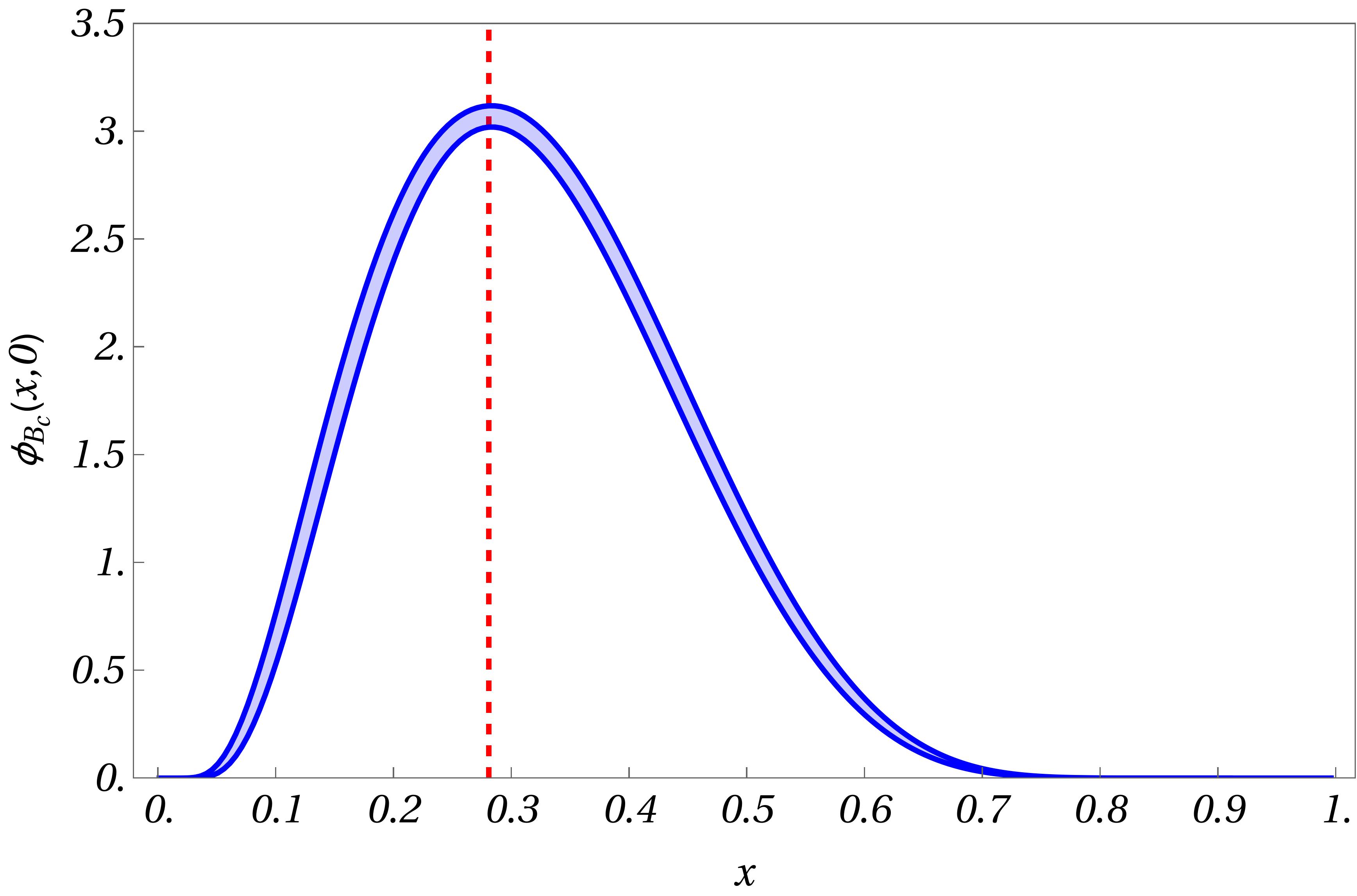
Figure 2: Shape of $B_{c}$ meson distribution amplitude with extracted value of $\omega_{B_{c}}$. The blue curve denotes $\phi_{B_{c}}(x,0)$ obtained using our extracted value of $\omega_{B_{c}}$ and the red dashed line denotes the point $x\sim m_{c}/m_{b}\sim 0.298(19)$.

With the LCDA parameters extracted, we now use them as inputs into the analytic expressions of the form factors showcased in appendix B and obtain our predictions for the form factors at $q^{2}=0$. In calculating the form factors, we set the cut-off of the impact parameter, $b_{c}$ in the form factor expressions at 90% of $1/\Lambda_{QCD}$. This is done to keep our predictions in a region well within maximum value of $b$ upto which pQCD is valid, i.e., $1/\Lambda_{QCD}$. These predictions are presented in Table 6 which are very much consistent with the lattice inputs used in the analysis.

Form Factors	This work	Lattice Input at $\boldsymbol{q^{2}=0}$Harrison:2020gvo
$F_{+}^{B_{c}\rightarrow\eta_{c}}(0)$	0.527(118)	-
$A_{0}^{B_{c}\rightarrow J/\psi}(0)$	0.452(39)	0.477(43)
$A_{1}^{B_{c}\rightarrow J/\psi}(0)$	0.439(32)	0.457(28)
$A_{2}^{B_{c}\rightarrow J/\psi}(0)$	0.411(68)	0.417(87)
$V^{B_{c}\rightarrow J/\psi}(0)$	0.746(57)	0.725(67)

Table 6: Prediction of form factors of $B_{c}\rightarrow J/\psi(\eta_{c})$ transition at $q^{2}=0$ and comparison with lattice values.

Thus to conclude in this section, we have extracted the shape parameters of $B_{c}$, $J/\psi$ and $\eta_{c}$ meson distribution amplitudes to be used during the predictions of form factors concerning $B_{c}\rightarrow\text{ }P$ wave charmonia in later sections.

4 Numerical analysis of some $B_{c}\rightarrow P$ wave semileptonic channels

Now that the analysis involving the decay of $B_{c}\rightarrow\text{ }S$ wave charmonium states is accomplished, in this section we move onto analyzing the $B_{c}\rightarrow P$ wave semileptonic decay channels. For these channels the information on the form factors are not available from lattice. Hence, it would be interesting to obtain the shapes of the form factors for further phenomenological studies. This void in present phenomenological arena motivates us to explore these decay channels and present predictions on some fundamental quantities such as the form factors and some physical observables like semileptonic branching ratios which can be verified in near future when sufficient inputs become available. In this section, our focus is primarily going to be on the scalar $\chi_{c0}$ and the axial-vector $\chi_{c1}$ and $h_{c}$ states. We are going to perform the analysis in three steps separated in three subsections. In the first step in subsection 4.1 we will be extracting the decay constants of the charmonium states. In the second step in subsection 4.2 we will be predicting the relevant form factors first at $q^{2}=0$ and then extrapolate them to full physical $q^{2}$ region utilising suitable extrapolation technique. And in the final step in subsection 4.3 we will be calculating and predicting a number of relevant physical observables utilising the form factor information obtained in the second step.

4.1 Extraction of decay constants of charmonium states

In this subsection, we extract the decay constants of $\chi_{c0}$, $\chi_{c1}$ and $h_{c}$ states, through a rather data driven approach, steering ourselves away from taking the currently available model dependent estimates as inputs. The primary motivation for doing so can be explained by revisiting eqs .˜34, 36 and 37. We can clearly see that unlike the LCDAs of $S$ wave charmonia, these do not have any shape parameters to introduce any degree of flexibility to their shapes. Even if they had such a parameter, extracting them would be difficult owing to the unavailability of sufficient data at present. Therefore, we consider the decay constants as a free parameter in the LCDAs and extract them following the approach discussed in the following text. Revisiting eqs .˜36 and 37 we make an assumption $f_{A}\approx f_{A}^{\perp}$ due to the lack of enough inputs available at present to extract them separately.

1. Extracting $\boldsymbol{f_{\chi_{c0}}}$: As for the theoretical expressions we consider the results presented by Li and Vary in their work Li:2021ejv , where they have presented the two photon decay width of $\chi_{c0}$ in Basis Light-Front Quantization (BLFQ) approach. In their work, they have expressed the transition amplitude for the process by parametrizing it in terms of two transition form factors (TFF)

   $$\begin{split}\mathcal{M}^{\mu\nu}=&\frac{4\pi\alpha}{M_{\chi_{c0}}^{2}}\Biggl{\{}M_{\chi_{c0}}^{2}\left[(q_{1}\cdot q_{2})g^{\mu\nu}-q_{2}^{\mu}q_{1}^{\nu}\right]F_{1}^{S}(q_{1}^{2},q_{2}^{2})+\\ &\left[q_{1}^{2}q_{2}^{2}g^{\mu\nu}+(q_{1}\cdot q_{2})q_{1}^{\mu}q_{2}^{\nu}-q_{1}^{2}q_{2}^{\mu}q_{2}^{\nu}-q_{2}^{2}q_{1}^{\mu}q_{1}^{\nu}\right]F_{2}(q_{1}^{2},q_{2}^{2})\Biggr{\}},\end{split}$$ (43)

   with $\alpha=1/137$. The subsequent two photon decay width can then be expressed as

   $$\Gamma_{S\rightarrow\gamma\gamma}=\frac{\pi\alpha^{2}}{4}M_{\chi_{c0}}^{3}|F_{1}^{S}(0,0)|^{2},$$ (44)

   considering both the photons are on-shell, and $F_{1}^{s}(0,0)$ represents the TFF in that case. In case if one of the photons is considered to be off-shell, the TFF would be a function of the momentum transferred, $Q^{2}$, which as has been expressed in Li:2021ejv will have the form

   $$F_{s\gamma}(Q^{2})=e_{c}^{2}f_{\chi_{c0}}\int_{0}^{1}\frac{(1-2x)\phi_{s}(x,\mu)}{x(1-x)Q^{2}+m_{f}^{2}}dx,$$ (45)

   $f_{\chi_{c0}}$ being the decay constant and $\phi_{s}(x,\mu)$ the leading twist LCDA of the $\chi_{c0}$ meson respectively, the form for which, in our work, has been considered to be the same as taken while calculating the for $B_{c}\rightarrow\chi_{c0}$ form factors. The branching ratio is expressed as

   $$\mathcal{B}(\chi_{c0}\rightarrow\gamma\gamma)=\frac{\Gamma(\chi_{c0}\rightarrow\gamma\gamma)}{\Gamma_{\chi_{c0}}},$$ (46)

   where $\Gamma_{\chi_{c0}}=10.8(6)$ MeV is the total decay width of $\chi_{c0}$ meson. Experimentally the numerical value of the branching ratio of the channel $\chi_{c0}\rightarrow\gamma\gamma$ has been determined to be 2.04(9)$\times 10^{-4}$Belle:2006mzv . With the expressions for the branching ratio and the corresponding experimental input at our hand we extract $f_{\chi_{c0}}$ and finally get

   $$f_{\chi_{c0}}=0.147(20).$$ (47)

2. Extracting $\boldsymbol{f_{\chi_{c1}}}$: Extracting $f_{\chi_{c1}}$ involves a bit more discussion since the process will involve a chi-square minimization taking three radiative decay channels of $\chi_{c1}$ as inputs. First we discuss the three channels used in this analysis in three separate bullet points and then present our final results.

   • Channel 1: $\chi_{c1}\rightarrow J/\psi\gamma$: This transition is an electric dipole (E1) transition, with the P wave charmonium state $\chi_{c1}$ decaying into an S wave charmonium state with the emission of a photon. Being an E1 transition, it involves a change in orbital angular momentum quantum number (L) by 1 while the spin quantum number (S) remains unchanged. The process follows E1 selection rules, allowing a change of $\Delta L=\pm 1$ and $\Delta J=0,\pm 1$ other than $J=0$ to $J=1$. The branching ratio for this process has been calculated using the potential NRQCD (pNRQCD) approach, where the transition amplitude depends on the overlap between the initial $\chi_{c1}$ and final $J/\psi$ state. In this framework, the branching ratio is expressed as MartinezNeira:2017prz

     $$\mathcal{B}(\chi_{c1}\rightarrow J/\psi\gamma)=\frac{1}{\Gamma_{\chi_{c1}}}\cdot\frac{4}{9}e_{c}^{2}\alpha\omega_{\chi_{c1}}^{3}|I_{SP}|^{2}\left(1+\delta^{\prime}\right),$$ (48)

     with $e_{c}$ representing the charge of the charm quark, $\omega_{\chi_{c1}}$ representing the energy of the emitted photon, $\Gamma_{\chi_{c1}}=0.84(4)$ MeV and $I_{SP}$ representing the overlap integral of the radial states of the participating mesons expressed as

     $$I_{SP}=\int_{0}^{\infty}r^{3}R_{S}(r)R_{P}(r)dr,$$ (49)

     where $R_{S}(r)$ and $R_{P}(r)$ represents the normalized radial solution of Schr$\ddot{o}$dinger equation for $J/\psi$ and $\chi_{c1}$ mesons respectively which in this work has been calculated by considering the potential binding the quark and anti-quark to be a Coulombic potential. The normalised radial solutions have the form

     $$\begin{split}R_{S}(r)&=\sqrt{\frac{q_{B_{S}}^{3}}{2}}\exp\left(-\frac{q_{B_{S}}r}{2}\right),\\ R_{P}(r)&=\sqrt{\frac{q_{B_{P}}^{5}}{24}}r\exp\left(-\frac{q_{B_{P}}r}{2}\right),\end{split}$$ (50)

     with $q_{B_{S}}$ and $q_{B_{P}}$ representing the Bohr momenta for S and P wave states respectively. To introduce decay constants into Eqn (48) we are going to express $q_{B_{S}}$ and $q_{B_{P}}$ interms of respective decay constants. The decay constants of $J/\psi$ and $\chi_{c1}$ can be expressed in terms of $R_{S}(0)$ and $R_{P}^{\prime}(0)$ as

     • For $J/\psi$ meson: The decay constant $f_{J/\psi}$ can be expressed in terms of necessary NLO and relativistic corrections by taking the expression for the decay width of $J/\psi\rightarrow e^{+}e^{-}$ channel in Bodwin:2002cfe and expressing the decay width as proportional to the square of the decay constant

       $$\scriptsize f_{J/\psi}=\sqrt{\frac{3}{2m_{c}\pi}}|R_{J/\psi}(0)|\left[1-\frac{8}{3}\frac{\alpha_{s}}{\pi}-\frac{1}{6}\langle v^{2}\rangle_{J/\psi}+\frac{\alpha_{s}}{3\pi}\left\{\frac{8}{9}+\frac{8}{9}\ln\left(\frac{\mu^{2}}{m_{c}^{2}}\right)\right\}\langle v^{2}\rangle_{J/\psi}+\frac{29}{18}\langle v^{4}\rangle_{J/\psi}\right],$$ (51)

       where $\alpha_{s}$ representing the running coupling constant has been calculated at scale $\mu=2m_{c}$. $\langle v^{2}\rangle_{J/\psi}$ represents the average of the square of relative velocity between the quark pair in the charmonium, it’s value being taken to be $\langle v^{2}\rangle_{J/\psi}=0.267$Zhu:2017lqu .

     • and for $\chi_{c1}$ meson: The expression for the decay constant of $\chi_{c1}$ in terms of $|R^{\prime}_{\chi_{c1}}|$ has been taken from Chung:2021efj and is expressed as

       $$f_{\chi_{c1}}=\sqrt{\frac{9N_{c}}{\pi M_{\chi_{c1}}}}\frac{|R_{\chi_{c1}}^{\prime}(0)|}{m_{c}}\left[1+\alpha_{s}c_{a}^{(1)}+\alpha_{s}^{2}c_{a}^{(2)}+\delta_{C}+\alpha_{s}c_{a}^{(1)}\delta_{C}+\delta_{NC}\right],$$ (52)

       where $c_{a}^{(1)}$ and $c_{a}^{(2)}$ represent the short distance coefficinets at order $\alpha_{s}$ and $\alpha_{s}^{2}$ respectively and their explicit expressions have been taken from Chung:2021efj . $\delta_{C}$ and $\delta_{NC}$ represent Coulombic and Non-Coulombic corrections to the binding potential respectively, and $\alpha_{s}$ has been calculated at the same scale as has been done for $J/\psi$. The expression for $f_{\chi_{c1}}$ in Chung:2021efj has two additional correction terms $\delta_{RS^{\prime}}$ and $\delta_{m_{RS^{\prime}}}$ which in this work we have neglected, since our analysis does not consider the charm quark mass to be in any particular renormalization scheme, but an average of the three schemes. Therefore, any correction term introduced which is renormalization scheme dependent has been neglected.

     Setting r=0 in Eqn (50) and putting them in Eqns (51) and (52), we can finally express the respective $q_{B}$ in terms of $f_{J/\psi}$ and $f_{\chi_{c1}}$. We get

     $$\scriptsize q_{B_{J/\psi}}=\left[\frac{4m_{c}\pi}{3}f_{J/\psi}^{2}\left\{1-\frac{8}{3}\frac{\alpha_{s}}{\pi}-\frac{1}{6}\langle v^{2}\rangle_{J/\psi}+\frac{\alpha_{s}}{3\pi}\left(\frac{8}{9}+\frac{8}{9}\ln\left(\frac{\mu^{2}}{m_{c}^{2}}\right)\right)\langle v^{2}\rangle_{J/\psi}+\frac{29}{18}\langle v^{4}\rangle_{J/\psi}\right\}^{-2}\right]^{1/3},$$ (53)

     and

     $$q_{B_{\chi_{c1}}}=\left[\frac{24\pi M_{\chi_{c1}}m_{c}^{2}}{9N_{c}}f_{\chi_{c1}}^{2}\frac{1}{|1+\alpha_{s}c_{a}^{(1)}+\alpha_{s}^{2}c_{a}^{(2)}+\delta_{C}+\alpha_{s}c_{a}^{(1)}\delta_{C}+\delta_{NC}|^{2}}\right]^{1/5}.$$ (54)

     Putting these equations in eqn.(50) we can express the radial solutions in terms of decay constants, using which we can, in turn, express the overlap integral in eqn.(49) and hence branching ratio in terms of the relevant decay constants. Going back to eqn.(48), the $\delta^{\prime}$ term which has been added to represent the relativistic corrections to leading order expression of the branching ratio. This correction term comprises of

     • Correction arising from higher order operators in pNRQCD Lagrangian.

     • Corrections arising due to the interference between the higher order terms to the initial and final quarkonium states.

     Details of the sources of these correction terms have been discussed in MartinezNeira:2017prz .

   • Channel 2: $\chi_{c1}\rightarrow V\gamma$: The $\chi_{c1}\rightarrow V\gamma$ transition, with V representing a light vector meson $\rho$ and $\phi$, is a radiative decay of charmonium involving the emission of a photon and the production of a light meson. These decays are different from E1 transition, the process involving a quark annihilation process, followed by hadronization of gluons into light meson. For the expression of decay width of the respective decay channel, we consider the analysis done by N. Kivel and M. Vanderhaegen in Kivel:2017nrw using QCD factorization approach. The decay width is expressed as

     $$\mathcal{B}(\chi_{c1}\rightarrow V\gamma)=\frac{1}{\Gamma_{\chi_{c1}}}\frac{1}{12\pi}\frac{\omega_{\chi_{c1}}^{5}}{M_{\chi_{c1}}^{4}}\left\{|\mathcal{A}_{1V}^{\parallel}|^{2}+|\mathcal{A}_{1V}^{\perp}|^{2}\right\},$$ (55)

     where $\mathcal{A}_{1V}^{\parallel}$ is the decay amplitude into longitudinal light meson and has the form as

     $$\mathcal{A}_{1V}^{\parallel}=-i\langle\mathcal{O}(\chi_{c1})\rangle\frac{f_{V}M_{\chi_{c1}}^{2}}{m_{c}^{6}}Q_{V}\sqrt{4\pi\alpha}\alpha_{s}^{2}\frac{N_{c}^{2}-1}{2N_{c}^{2}}\int_{0}^{1}dx\phi_{V}^{\parallel}(x)T_{1}(x),$$ (56)

     with the hard kernel

     $$T_{1}(x)=\text{Re }T_{1}(x)+\text{Im }T_{1}(x),$$ (57)

     with the explicit expressions of $\text{Re }T_{1}(x)$ and $\text{Im }T_{1}(x)$ has been taken from Kivel:2017nrw and the twist 2 distribution amplitude of the light vector meson $\phi_{V}^{\parallel}(x)$ has the form

     $$\phi_{V}(x,\mu)=6x(1-x)\left\{1+a_{2}^{V}(\mu)C_{2}^{3/2}(2x-1)\right\},$$ (58)

     with the coefficient $a_{2}^{V}(\mu)$ defined at scale $\mu$. In addition, $A_{1V}^{\perp}$ representing the decay amplitude into tranverse light meson is expressed as

     $$\begin{split}\mathcal{A}_{1V}^{\perp}=i\langle\mathcal{O}(\chi_{c1})\rangle&\frac{f_{V}m_{V}}{m_{c}^{5}}\frac{M_{\chi_{c1}}^{2}}{m_{c}^{2}}\sqrt{4\pi\alpha}\frac{\pi\alpha_{s}}{N_{c}}\int D\alpha_{i}\biggl{\{}\delta_{I0}9e_{Q}\frac{G(\alpha_{i})}{\alpha_{1}\alpha_{2}\alpha_{3}^{2}}\\ &-\frac{Q_{V}}{4}\left(\frac{\alpha_{1}-\alpha_{2}}{\alpha_{1}\alpha_{2}\alpha_{3}^{2}}V(\alpha_{i})+\frac{1-\alpha_{3}}{\alpha_{1}\alpha_{2}\alpha_{3}^{2}}A(\alpha_{i})\right)\biggr{\}},\end{split}$$ (59)

     with

     $$\int D\alpha_{i}f(\alpha_{i})=\int_{0}^{1}d\alpha_{1}\int_{0}^{1}d\alpha_{2}\int_{0}^{1}d\alpha_{3}\delta(1-\alpha_{1}-\alpha_{2}-\alpha_{3})f(\alpha_{1},\alpha_{2},\alpha_{3}),$$ (60)

     and $A(\alpha_{i})$, $V(\alpha_{i})$ and $G(\alpha_{i})$ are twist 3 distribution amplitudes and have the form asKivel:2017nrw

     $$\begin{split}A(\alpha_{i})&=360\zeta_{3}\alpha_{1}\alpha_{2}\alpha_{3}^{2}\left(1+\omega_{3}^{A}\frac{1}{2}(7\alpha_{3}-3)\right),\\ V(\alpha_{i})&=540\zeta_{3}\omega_{3}^{V}\alpha_{1}\alpha_{2}\alpha_{3}^{2}(\alpha_{2}-\alpha_{1}),\\ G(\alpha_{i})&=5040\zeta_{3}\omega_{3}^{G}\alpha_{1}^{2}\alpha_{2}^{2}\alpha_{3}^{2},\end{split}$$ (61)

     with $\zeta_{3}$, $\omega_{3}^{A,V,G}$ being the non-perturbative parameters of the twist 3 DAs with the scale $\mu$ set at $\mu=2m_{c}$ and the evolution of the parameters from $\mu=1.0$ GeV to $2m_{c}$ has been taken from Kivel:2017nrw . In eqns.(56) and (59) $f_{V}$ represent the decay constant of the light meson having the values

     $$f_{\rho}=0.221\text{ }GeV,\qquad f_{\phi}=0.161\text{ }GeV,$$ (62)

     Channel	Values
     $\chi_{c1}\rightarrow J/\psi\gamma$	34.3(1.3)%
     $\chi_{c1}\rightarrow\rho^{0}\gamma$	2.16(17)$\times 10^{-4}$
     $\chi_{c1}\rightarrow\phi\gamma$	2.4(5)$\times 10^{-5}$

     Table 7: Inputs used to extract $f_{\chi_{c1}}$.

     and other parameters include $e_{Q}=2/3$, the charge of the heavy quark, $Q_{V}$ represents an appropriate combination of the quark charges

     $$Q_{\rho^{0}}=\frac{1}{2}(e_{u}-e_{d})=\frac{1}{2},\qquad Q_{\phi}=e_{s}=-\frac{1}{3},$$ (63)

     $m_{V}$ represents the mass of the light vector mesons having values

     $$m_{\rho}=0.775\text{ }GeV,\qquad m_{\phi}=1.019\text{ }GeV,$$ (64)

     and the NRQCD matrix element $\langle\mathcal{O}(\chi_{c1})\rangle$ is related to $R^{\prime}(0)$ as

     $$\langle\mathcal{O}(\chi_{c1})\rangle=\sqrt{2N_{c}}\sqrt{2M_{\chi_{c1}}}\sqrt{\frac{3}{4\pi}}R_{\chi_{c1}}^{\prime}(0),$$ (65)

     where we again substitute $R^{\prime}(0)$ using eqn.(52) to introduce $f_{\chi_{c1}}$ into the expression.

   With the above expressions for the branching ratios and corresponding inputs from Table 7 we construct a chi-square function. As for the nuisance parameters, we take the prior estimates of $f_{J/\psi}$, $m_{c}$ and $\Lambda$ from Table 5, that of Coulombic and Non-Coulombic corrections terms from Chung:2021efj with a 10% error as

   $$\delta_{C}=0.266(27),\qquad\delta_{NC}=0.493(49),$$ (66)

   and that of the coefficints of twist-2 and twist-3 DAs at $\mu=1.0$ GeV asKivel:2017nrw

   $$a_{2\rho}=0.15(7), a_{2\phi}=0.18(8),$$

   $$\zeta_{\rho}=0.03(1), \zeta_{\phi}=0.024(8),$$

   $$\omega_{\rho}^{A}=-3.0(1.4), \omega_{\phi}^{A}=-2.6(1.3),$$

   $$\omega_{\rho}^{V}=5.0(2.4), \omega_{\phi}^{V}=5.3(3.0).$$

   With these inputs, once the chi-square function is constructed, we optimize it to finally extract $f_{\chi_{c1}}$ which we present in Table 8, along-with the corresponding correlation matrix between the extracted parameters in Table 20.

   Free Parameters		Nuisance Parameters
   Parameters	Fit Results	Parameters	Fit Results
   $f_{\chi_{c1}}$	0.169(28)	$f_{J/\psi}$	0.405(3)
   $\delta^{\prime}$	-0.624(22)	$m_{c}$	1.342(31)
   		$\Lambda$	0.2789(8)
   		$\Gamma_{\chi_{c1}}$	0.840(28)
   		$\delta_{C}$	0.266(18)
   		$\delta_{NC}$	0.493(35)
   		$a_{2\rho}(\mu=1.0)$	0.154(49)
   		$a_{2\phi}(\mu=1.0)$	0.172(56)
   		$\zeta_{\rho}(\mu=1.0)$	0.033(6)
   		$\zeta_{\phi}(\mu=1.0)$	0.023(6)
   		$\omega_{\rho}^{A}(\mu=1.0)$	-3.85(89)
   		$\omega_{\rho}^{V}(\mu=1.0)$	2.11(88)
   		$\omega_{\phi}^{A}(\mu=1.0)$	-2.60(99)
   		$\omega_{\phi}^{V}(\mu=1.0)$	5.30(2.12)
   D.O.F	1
   p-Value	15.36%

   Table 8: Extracted value of decay constant of $\chi_{c1}$ meson, along-with estimates of other relevant parameters.

3. Extracting $\boldsymbol{f_{h_{c}}}$: Extracting $f_{h_{c}}$ is comparatively straightforward due to the unavailibity of enough decay channels to be considered as inputs. We take a single decay channel, namely $h_{c}\rightarrow\eta_{c}\gamma$ radiative channel for this purpose. Being an E1 transition, the branching ratio for this channel can also be calculated in pNRQCD framework, the expression being the same as we had previously shown for $\chi_{c1}\rightarrow J/\psi\gamma$. The expression for the branching ratio is as

   $$\mathcal{B}(h_{c}\rightarrow\eta_{c}\gamma)=\frac{1}{\Gamma_{h_{c}}}\cdot\frac{4}{9}e_{c}^{2}\alpha\omega_{h_{c}}^{3}|I_{SP}|^{2}\left(1+\delta^{\prime}\right),$$ (67)

   with $\Gamma_{h_{c}}=0.78(28)\text{ }MeV$ being the total width of $h_{c}$ meson, $e_{c}$, $\alpha$ and $\omega_{h_{c}}$ having the same meaning as has been discussed before. $I_{SP}$ represents the overlap integral between the initial $h_{c}$ state and the final $\eta_{c}$ state wavefunctions. The general expression for the overlap integral, and its expression in terms of the decay constant is the same as we had calculated for $\chi_{c1}\rightarrow J/\psi\gamma$. $f_{h_{c}}$ can be incorporated into the expression for overlap integral same as before utilising eqn. (52) with $\chi_{c1}$ being replaced by $h_{c}$ in this case and the estimates of Coulombic and Non-Coulombic correction terms taken from Table 8. As for $\eta_{c}$ meson, the decay constant can be connected to $R_{\eta_{c}}(0)$, the radial wave function at origin as

   $$\begin{split}f_{\eta_{c}}=\sqrt{\frac{3}{2m_{c}\pi}}R_{\eta_{c}}(0)\biggl{[}&1+\frac{\alpha_{s}(\mu)}{\pi}\frac{\pi^{2}-20}{3}+\langle v^{2}\rangle_{\eta_{c}}\biggl{\{}-\frac{4}{3}+\frac{\alpha_{s}(\mu)}{\pi}\frac{1}{27}(48\ln(\frac{\mu^{2}}{m_{c}^{2}})-96\ln 2\\ &-15\pi^{2}+196)\biggr{\}}+\frac{68}{45}\langle v^{4}\rangle_{\eta_{c}}\biggr{]}^{1/2},\end{split}$$ (68)

   by expressing the decay width of $\eta_{c}\rightarrow\gamma\gamma$ radiative channel derived in Guo:2011tz as proportional to the square of $f_{\eta_{c}}$. Following the same procedure as previously shown in eqns. (50) and (53), we arrive at $q_{B_{\eta_{c}}}$ in terms of $f_{\eta_{c}}$ as

   $$\begin{split}q_{B_{\eta_{c}}}=\biggl{[}\frac{4m_{c}\pi}{3}f_{\eta_{c}}^{2}\biggl{[}&1+\frac{\alpha_{s}(\mu)}{\pi}\frac{\pi^{2}-20}{3}+\langle v^{2}\rangle_{\eta_{c}}\biggl{\{}-\frac{4}{3}+\frac{\alpha_{s}(\mu)}{\pi}\frac{1}{27}(48\ln(\frac{\mu^{2}}{m_{c}^{2}})-96\ln 2\\ &-15\pi^{2}+196)\biggr{\}}+\frac{68}{45}\langle v^{4}\rangle_{\eta_{c}}\biggr{]}^{-1}\biggr{]}^{1/3},\end{split}$$ (69)

   with $\alpha_{s}$ being calculated at $\mu=2m_{c}$, $\Lambda$ taken from Table 8 and $\langle v^{2}\rangle_{\eta_{c}}=0.267$. The correction term $\delta^{\prime}$ has the same meaning as for the former channel and its value has been taken from Table 8 as inputs into eqn.(67). As for the value of $f_{\eta_{c}}$ we take the estimate previously extracted in Table 5 as input. Finally we extract $f_{h_{c}}$ by solving eqn. (67) with experimentally observed value of the branching ratio, i.e., $\mathcal{B}(h_{c}\rightarrow\eta_{c})_{exp}=60(4)\%$ParticleDataGroup:2022pth and arrive at

   $$f_{h_{c}}=0.182(47).$$ (70)

4.2 Prediction of $B_{c}\rightarrow\text{ }P$ wave semileptonic form factors

Following the extraction of $f_{\chi_{c0}}$, $f_{\chi_{c1}}$ and $f_{h_{c}}$, we are now in a position to calculate the $B_{c}\rightarrow P$ wave semileptonic form factors. First we calculate the relevant form factors at $q^{2}=0$ through the modified pQCD approach. Once we have the form factors at $q^{2}=0$, we then extrapolate them to $q_{max}^{2}$ through extrapolation technique discussed in subsequent text in this subsection. After introducing the extrapolation technique, we then actually extract the relevant extrapolation parameters, essentially using the inputs on $B_{c}\rightarrow\text{ }S$ wave form factor, motivation for which has been discussed in the text, and then propagate the thus extracted parameters to predict the $B_{c}\rightarrow\text{ }P$ wave form factors.

Form factors at $\boldsymbol{q^{2}=0}$:

With the estimates of the decay constants extracted in the previous subsection and that of the shape parameter of $B_{c}$ meson, $\omega_{B_{c}}$, and other relevant parameters from Table 5, we take them as inputs in the expressions for the form factors in modified pQCD shown in Appendix B and calculate the numerical values of the relevant form factors at $q^{2}=0$. Similar to what we did while calculating the form factors in Table 6, here too we consider a cut-off in the upper limit of impact parameter used in the pQCD expressions of form factors, $b_{c}$ at 90% of $1/\Lambda_{QCD}$. The predicted values of the form factors at thus calculated are presented in Table 9.

Decay	Form	This	Previous	QCDSR	LFQM	NRQCD
Channel	Factor	work	pQCDPhysRevD.98.033007	(Azizi:2009ny, )	Wang:2009mi	Zhu:2017lwi
$B_{c}\rightarrow\chi_{c0}$	$F_{+}(0)$	0.431(70)	0.41${}^{+0.09}_{-0.08}$	0.673(195)	$0.47^{+0.03}_{-0.06}$	$1.25^{+0.15}_{-0.12}$
	$A_{0}(0)$	0.166(26)	0.18${}^{+0.03}_{-0.03}$	0.03(1)	$0.13^{+0.01}_{-0.01}$	$0.12^{+0.01}_{-0.01}$
	$A_{1}(0)$	0.583(119)	0.86${}^{+0.17}_{-0.16}$	0.30(9)	$0.85^{+0.02}_{-0.04}$	$2.34^{+0.21}_{-0.22}$
$B_{c}\rightarrow\chi_{c1}$	$A_{2}(0)$	0.054(16)	0.11${}^{+0.02}_{-0.01}$	0.06(2)	$0.15^{+0.01}_{-0.01}$	$0.47^{+0.07}_{-0.06}$
	$V(0)$	0.290(48)	0.18${}^{+0.04}_{-0.04}$	0.13(4)	$0.36^{+0.02}_{-0.04}$	$0.99^{+0.19}_{-0.15}$
	$A_{0}(0)$	0.322(61)	0.22${}^{+0.05}_{-0.03}$	0.03(1)	$0.64^{+0.10}_{-0.02}$	$1.63^{+0.25}_{-0.19}$
	$A_{1}(0)$	0.761(188)	0.46${}^{+0.07}_{-0.07}$	0.30(9)	$0.50^{+0.05}_{-0.08}$	$0.46^{+0.07}_{-0.03}$
$B_{c}\rightarrow h_{c}$	$A_{2}(0)$	-0.023(10)	-0.03${}^{+0.0}_{-0.01}$	0.06(2)	$-0.32^{+0.06}_{-0.05}$	$-0.75^{+0.17}_{-0.17}$
	$V(0)$	0.323(77)	0.10${}^{+0.02}_{-0.01}$	0.13(4)	$0.07^{+0.00}_{-0.01}$	$0.07^{+0.00}_{-0.01}$

Table 9: Prediction of form factors of $B_{c}\rightarrow$ P wave transition at $q^{2}=0$.

From Table 9 we see that the error estimates of the form factors range from a minimum of 15.66% for $A_{0}(0)$ of $B_{c}\rightarrow\chi_{c1}$ channel to a maximum of 43.47% for $A_{2}(0)$ of $B_{c}\rightarrow h_{c}$ channel. The reason for the error estimate being comparatively larger than $B_{c}\rightarrow J/\psi(\eta_{c})$ channels is primarily due to the large error estimate of the decay constants, being about 13.60%, 16.56% and 25.82% for $f_{\chi_{c0}}$, $f_{\chi_{c1}}$ and $f_{h_{c}}$ respectively. Availability of information on branching ratios of more radiative decay channels of P wave charmonia or other inputs such as moments of charmonium LCDAs in future might help us better constrain the decay constants, thereby enabling us to predict the form factors to a greater degree of precision.

Extrapolation of form factors over full semileptonic region:

Having extracted the form factor information at $q^{2}=0$, the next course of action is to extrapolate the form factors to full physical $q^{2}$ region. The pCQD framework in itself is more reliable at the lower $q^{2}$ region, specifically in the range of about $0.0$ to $0.2(m_{B_{c}}-m)^{2}$Rui:2016opu . But as we saw in subsection 2.1, prediction of the physical observables require information of the form factors over the full physical $q^{2}$ region. Thus in order to make our predictions of form factors reliable over the full $q^{2}$ region, we need to extrapolate it to the high $q^{2}$ region. There are a number of extrapolation techniques available in literature that has been used previously. We use the two parameter pole expansion parametrization considered in Melikhov:2000yu for our work, which has the form as

$$f_{i}(q^{2})=\frac{f_{i}(0)}{P_{i}(q^{2})\left(1-\alpha_{i}\frac{q^{2}}{M_{i}^{2}}+\beta\frac{q^{4}}{M_{i}^{4}}\right)},$$ (71)

where $\alpha_{i}$ and $\beta$ represent the parameters that we intend to extract and $M_{i}$ represents the masses of the low-lying $B_{c}$ resonances. Their values have been taken from Leljak:2019eyw and has been shown in Table 10. The form factors $f_{i}(q^{2})$ have an additional weight factor $P_{i}(q^{2})$ having the form

$$P_{i}(q^{2})=1-\frac{q^{2}}{M_{i}^{2}},$$ (72)

which accounts for the contributions due to low-lying resonances present below the threshold production of $B_{c}-V$ pairs at $q^{2}=(m_{B_{c}}+m_{V})^{2}$, V representing final charmonium state. The inclusion of $P(q^{2})$ into the parametrization equations for all the form factors is justified as the resonance points for each of the masses presented in Table 10 lies well below the pair production threshold.

Note that the slope of the shapes of the form factors will be highly dependent on the respective masses of the low-lying resonances. The parameter $\alpha_{i}$ being the leading order coefficient in $q^{2}$ is taken to be different for each form factor. In contrast, for simplicity, the parameter $\beta$ being subleading in $q^{2}$ and only exhibiting control over the form factors at the very end of the semileptonic region is considered the same for all the form factors.

Form Factor	$F_{+}$	$F_{0}$	$A_{0}$	$A_{1}$	$A_{2}$	V
$M_{i}$ in GeV	6.34	6.71	6.28	6.75	6.75	6.34

Table 10: Masses of the low lying $B_{c}$ resonances.

The primary objective of this section is to extract the pole expansion parameters introduced in eq .˜71 utilising the $B_{c}\rightarrow J/\psi$ and $B_{c}\rightarrow\eta_{c}$ form factors as inputs, and then use the same extracted parameters to obtain information on $B_{c}\rightarrow\text{ }P$ wave form factors. To do this, a chi-square function is constructed with the form factor inputs at certain discreet $q^{2}$ points shown in Table 17 in Appendix D and then minimized to extract the required pole expansion parameters. The parameters thus extracted are shown in Table 11 and the correlation between the thus extracted parameters has been shown in Table 19.

Parameters	Fit Results
$\alpha_{A_{0}}$	1.600(138)
$\alpha_{A_{1}}$	1.553(121)
$\alpha_{A_{2}}$	1.589(255)
$\alpha_{V}$	1.647(124)
$\alpha_{F_{0}}$	0.916(287)
$\alpha_{F_{+}}$	1.465(197)
$\beta$	1.063(218)
D.O.F	9
p-Value	95.14%

Table 11: Results of extraction of Pole expansion parameters of $B_{c}\rightarrow J/\psi(\eta_{c})$ form factors.

The $q^{2}$ distribution of the form factors can be easily determined with the pole expansion parameters extracted. To check the predictivity of our fit, we have reproduced the $q^{2}$ distributions of the $B_{c}\to\eta_{c}$ and $B_{c}\to J/\psi$ form factors which we have shown in the plots of Fig. 11 (appendix), respectively. The predicted $q^{2}$ shapes comfortably explain all the inputs used in the fits.

As for the $q^{2}$ distribution of $B_{c}\rightarrow\text{ }P$ wave semileptonic form factors, we are going to utilise the same pole expansion parametrisation already discussed in eq .˜71. We have mentioned earlier that the slope of the $q^{2}$ shapes of the form factors is highly dependent on the low-lying resonances. Therefore, as an approximate approach, we have utilised the connection between the total angular momentum of the final meson states, enabling us to connect the slope of the form factors of $P$ wave scalar state, $\chi_{c0}$ with $S$ wave pseudoscalar state, $\eta_{c}$, both having total angular momentum $J=0$, and also the form factors of $P$ wave axial-vector meson states, $\chi_{c1}$ and $h_{c}$ with S wave vector meson state, $J/\psi$, both having total angular momentum $J=1$ Hernandez:2006gt ; Ivanov:2005fd . For simplicity, the parameter $\beta$ stays the same for all the form factors, while we take $\alpha_{F_{+}}$ and $\alpha_{F_{0}}$ given in table 11 as inputs to extrapolate the $B_{c}\rightarrow\chi_{c0}$ form factors. On the other hand, we have used $\alpha_{A_{0,1,2}}$ and $\alpha_{V}$ given in table 11 as inputs to extrapolate the $B_{c}\rightarrow\chi_{c1}(h_{c})$ form factors. The $q^{2}$ distribution of the form factors thus obtained through extrapolation has been shown in Figs. 3, 4 and 5 which can be tested once we have results from lattice.

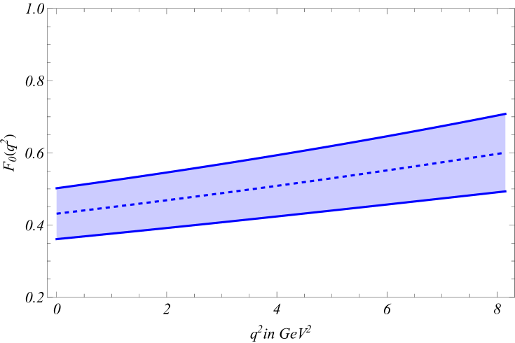
(a)

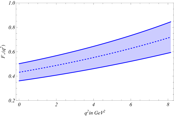
(b)

Figure 3: Plots showing the $q^{2}$ dependence of $B_{c}\rightarrow\chi_{c0}$ semileptonic form factors.

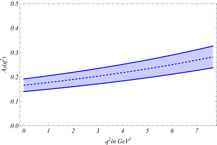
(a)

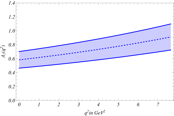
(b)

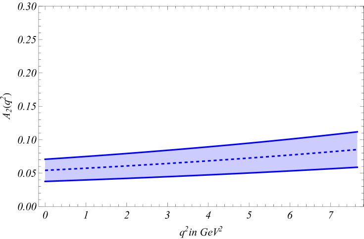
(c)

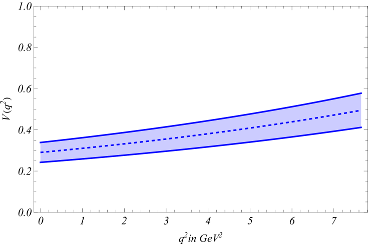
(d)

Figure 4: Plots showing the $q^{2}$ dependence of $B_{c}\rightarrow\chi_{c1}$ semileptonic form factors.

(a)

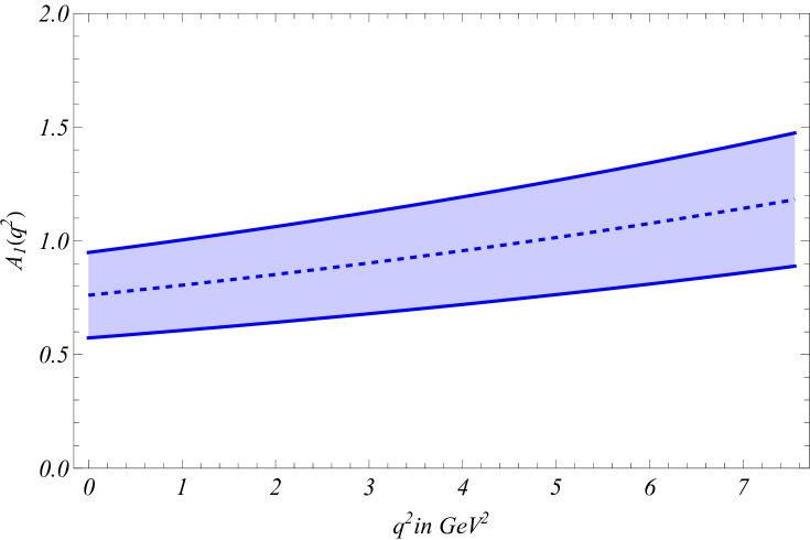
(b)

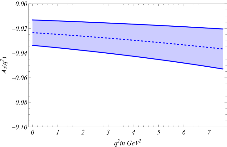
(c)

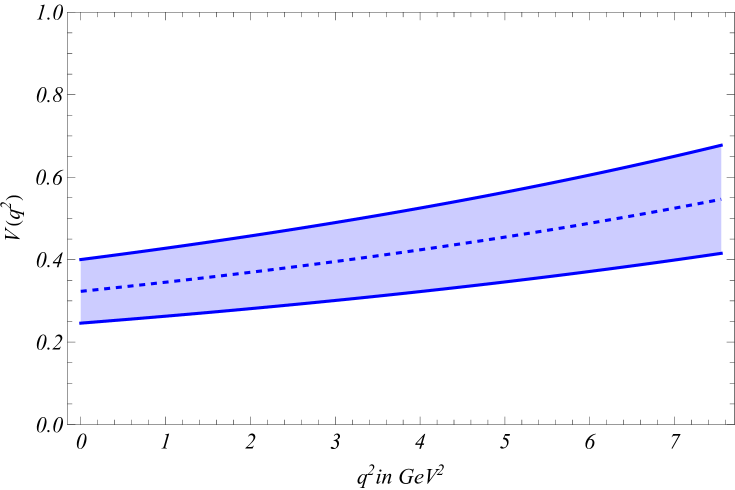
(d)

Figure 5: Plots showing the $q^{2}$ dependence of $B_{c}\rightarrow h_{c}$ semileptonic form factors.

4.3 Prediction of some physical observables

With information of form factors over the entire physical $q^{2}$ obtained, we are now in a position to perform predictions on some of the relevant physical observables. These include the branching ratios of some of the semileptonic transitions involving the emission of both light as well as heavy lepton, ratios of the respective branching ratios, and an angular observables, the forward backward asymmetry. The explicit expressions for the $q^{2}$ distribution of these observables have already been shown in subsection 2.1.

• In Fig 12 we showcase $q^{2}$ distribution of $B_{c}\rightarrow\chi_{c0},\chi_{c1}$ and $h_{c}$ semileptonic decay widths. In Table 12 we present our predictions of the branching ratios, obtained by integrating the differential decay width over the physical $q^{2}$ region, along-with comparison with predictions from other approaches. In the second column the actual error estimates obtained in PhysRevD.98.033007 are added up in quadrature and shown here.

  Decay Channels	This work	Previous pQCDPhysRevD.98.033007	QCDSRAzizi:2009ny	LFQMWang:2009mi
  $\mathcal{B}(B_{c}\rightarrow\chi_{c0}l\nu_{l})$	2.00(65)	2.22${}^{+1.18}_{-0.83}$	1.82(51)	$2.1^{+0.2}_{-0.4}$
  $\mathcal{B}(B_{c}\rightarrow\chi_{c0}\tau\nu_{\tau})$	0.339(114)	0.48${}^{+0.25}_{-0.18}$	0.49(16)	$0.24^{+0.01}_{-0.03}$
  $\mathcal{B}(B_{c}\rightarrow\chi_{c1}l\nu_{l})$	1.39(51)	1.53${}^{+0.69}_{-0.54}$	1.46(42)	$1.4^{+0.0}_{-0.1}$
  $\mathcal{B}(B_{c}\rightarrow\chi_{c1}\tau\nu_{\tau})$	0.170(65)	0.20${}^{+0.09}_{-0.06}$	0.147(44)	$0.15^{+0.01}_{-0.02}$
  $\mathcal{B}(B_{c}\rightarrow h_{c}l\nu_{l})$	2.61(1.16)	1.06${}^{+0.31}_{-0.32}$	1.42(40)	$3.1^{+0.5}_{-0.8}$
  $\mathcal{B}(B_{c}\rightarrow h_{c}\tau\nu_{\tau})$	0.259(115)	0.13${}^{+0.03}_{-0.04}$	0.137(38)	$0.22^{+0.02}_{-0.04}$

  Table 12: Branching ratios ($\times 10^{-3}$) of some $B_{c}\rightarrow P$ wave semileptonic channels predicted in this work along-with comparison with other predictions in existing literature.

  Checking Table 12 we can see that our predictions have attained values that agree well to the existing predictions within the error bars. However a comparison between our predictions to the previous pQCD predictionsPhysRevD.98.033007 shows an improvement of 49.9%, 47.9%, 35.5% and 30.5% for the first four rows respectively. But there is an increase in error estimate in the last two rows. Additionally the error estimates for the last two channels are higher compared to that of the other channels. The reason can be traced back to Table 9 where the error estimates of our $B_{c}\rightarrow h_{c}$ form factors are larger than the corresponding previous pQCD predictions and also to our $B_{c}\rightarrow\chi_{c1}$ form factor predictions. In all the predictions the electron and muon modes have not been differentiated due to both of them having small masses and not coming up with any significant difference in the values of the observables. However comparing the light lepton modes to the heavy tau lepton mode, we can see a significant drop in the values for the later. This is mainly due to a suppression coming from the phase space for the heavy lepton channels. Next we calculate ratios of the branching fraction $R(X)$, where $X$ is the final state charmonium. The general expression for $R(X)$ is as

  $$R(X)=\frac{\mathcal{B}(B_{c}\rightarrow X\tau\nu_{\tau})}{\mathcal{B}(B_{c}\rightarrow Xl\nu_{l})}.$$ (73)

  These ratios are much more cleaner observables compared to the branching ratios due to the reduction of theoretical uncertainties coming from the form factors. Our predictions along-with comparison with predictions from previous pQCD approach are shown in Table 13.

  Ratios	This work	Previous pQCDPhysRevD.98.033007
  $R(\chi_{c0})$	0.169(11)	0.22${}^{+0.0}_{-0.01}$
  $R(\chi_{c1})$	0.126(2)	0.13${}^{+0.01}_{-0.0}$
  $R(h_{c})$	0.113(3)	0.12${}^{+0.01}_{-0.0}$

  Table 13: Predictions for $R(\chi_{c0,1})$ and $R(h_{c})$ and comparison with existing predictions.

  We can see a significant reduction in error estimate in all the three ratios compared to the previous pQCD predictions. The central values typically lie between 0.113 and 0.169 which is significantly smaller than SM predictions of $R(\eta_{c})$ and $R(J/\psi)$. It would be interesting however to see if future measurements could indicate towards any possible anomaly in its values, just like $R(J/\psi)$. If so, it could in future hint towards possible NP effects, opening up a new arena to explore.

• Along-with the predictions of branching fractions, we also present predictions of tau lepton polarization $\langle P_{\tau}\rangle$, $\chi_{c1}(h_{c})$ longitudinal polarization fraction $\langle F_{L}\rangle$ and forward backward asymmetry $\langle A_{FB}(l(\tau))\rangle$, explicit expressions for which has already been discussed in section 2.1, in Table 14 for both light lepton and heavy lepton cases.

  

  (a)

  

  (b)

  

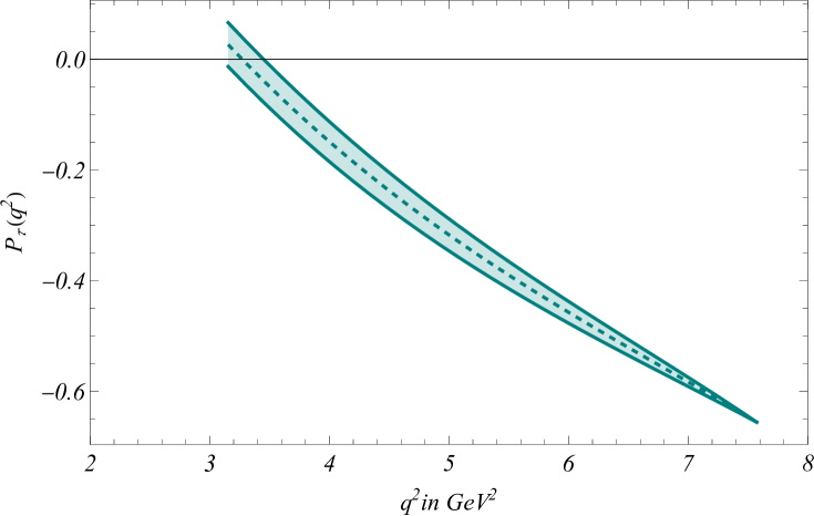
  (c)

  Figure 6: $q^{2}$ distribution of $P_{\tau}(q^{2})$ for (a)$B_{c}\rightarrow\chi_{c0}$, (b) $B_{c}\rightarrow\chi_{c1}$ and (c) $B_{c}\rightarrow h_{c}$ semitauonic channels.

  

  (a)

  

  (b)

  

  (c)

  

  (d)

  Figure 7: $q^{2}$ distribution of $F_{L}(q^{2})$. Plots (a) and (b) are for $B_{c}\rightarrow\chi_{c1}$ and (c) and (d) are for $B_{c}\rightarrow h_{c}$ semileptonic channels. The violet and green plots denote the light lepton and heavy lepton cases respectively.

  

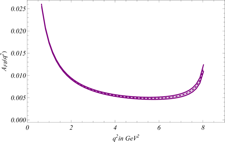
  (a)

  

  (b)

  

  (c)

  

  (d)

  

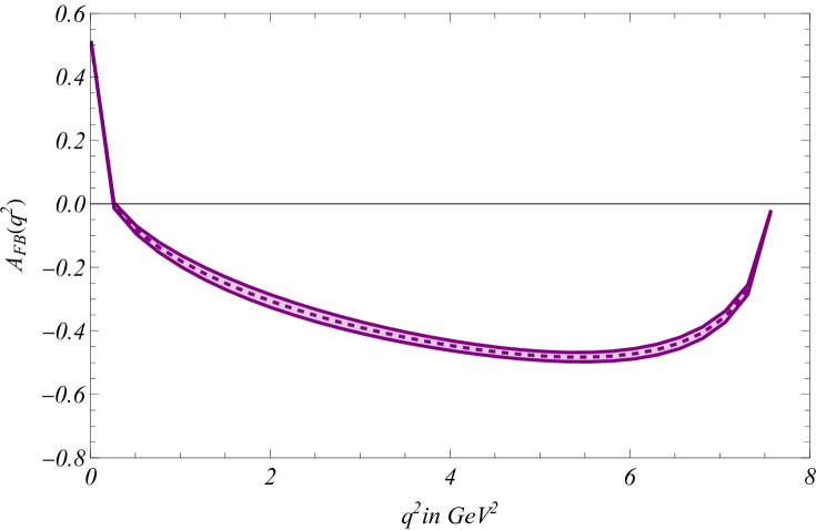
  (e)

  

  (f)

  Figure 8: $q^{2}$ distribution of $A_{FB}(q^{2})$. Plots (a) and (b) are for $B_{c}\rightarrow\chi_{c0}$, (c) and (d) are for $B_{c}\rightarrow\chi_{c1}$ and (e) and (f) are for $B_{c}\rightarrow h_{c}$ semileptonic channels. The violet and green plots denote the light lepton and heavy lepton cases respectively.

  Channel	$\boldsymbol{\langle P_{\tau}\rangle}$	$\boldsymbol{\langle F_{L}(l)\rangle}$	$\boldsymbol{\langle F_{L}(\tau)\rangle}$	$\boldsymbol{\langle A_{FB}(l)\rangle}$	$\boldsymbol{\langle A_{FB}(\tau)\rangle}$
  $B_{c}\rightarrow\chi_{c0}$	0.507(37)	-	-	0.0185(5)	0.374(8)
  $B_{c}\rightarrow\chi_{c1}$	-0.498(19)	0.315(16)	0.307(8)	-0.490(11)	-0.300(11)
  $B_{c}\rightarrow h_{c}$	-0.415(23)	0.490(24)	0.417(23)	-0.362(18)	-0.172(25)

  Table 14: Predictions on $\langle P_{\tau}\rangle$, $\langle F_{L}\rangle$ and $\langle A_{FB}\rangle$ in SM framework for $B_{c}\rightarrow P$ wave channels.

  Checking Table 14, in the second column we can see that $\langle P_{\tau}\rangle$ for $\chi_{c0}$ is positive while that for $\chi_{c1}$ and $h_{c}$ are negative. This is because of the dominance of decay width with tau lepton helicity +1/2 over that with helicity -1/2 for the former case, while for the later case the production of tau lepton with helicity -1/2 is favoured over one with helicity +1/2. In the third and fourth columns comparing the $\langle F_{L}\rangle$, the value for $h_{c}$ is greater than that for $\chi_{c1}$. The reason can be traced back to the helicity amplitudes, mainly $H_{V0}$ which contributes to $\Gamma_{0}$ in the numerator of eq .˜17. $H_{V0}$ inturn depends on $A_{1}$ and $A_{2}$ which for $B_{c}\rightarrow\chi_{c1}$ carry the same sign, hence resulting in a destructive interference between the two, while for $B_{c}\rightarrow h_{c}$ the two form factors carry opposite sign resulting in a constructive interference, thus resulting in a higher value. Also the differences between values for tau and light-lepton channels are small when checked for both $\chi_{c1}$ and $h_{c}$ modes, suggesting that longitudinal polarization fraction still favours lepton flavor universality to some extent. In the fifth and sixth columns $\langle A_{FB}\rangle$ is positive for $\chi_{c0}$ while it is negative for $\chi_{c1}$ and $h_{c}$. This signifies that the lepton-neutrino pair is more preferebly emitted in forward direction relative to the $B_{c}$ meson for $B_{c}\rightarrow\chi_{c0}$ channel, and more preferebly in the backward direction for $B_{c}\rightarrow\chi_{c1}(h_{c})$ channels. As for the error estimtates, similar to Table 15, here too we get a significant reduction in error, ranging from a minimum of about 2% to a maximum of about 14%, the reason primarily being the cancellation of errors coming from all the relevant form factors.

  Coming to the plots, Fig 6 showcases $q^{2}$ distribution of $P_{\tau}$ where in every plot we can see its magnitude increasing as we move from low $q^{2}$ to high $q^{2}$. This happens due to (a) the additional $(m_{l}^{2}/2q^{2})$ term in $d\Gamma_{+}/dq^{2}$ which suppresses it at high $q^{2}$, and (b) the helicity term $3(H_{V,t}^{s})^{2}$ which falls faster with increasing $q^{2}$ compared to $(H_{V,0}^{s})^{2}$, inturn making the denominator in eq .˜14 fall faster with increasing $q^{2}$ compared to the numerator, thereby increasing its value with increasing $q^{2}$.

  Next in Fig 7 we showcase the $q^{2}$ distribution of $F_{L}$ where the curve initially falls as $q^{2}$ increases and then rises slightly near $q_{max}^{2}$. This can be explained from eq .˜17 where as $q^{2}$ initially increases, $\Gamma^{+1}+\Gamma^{-1}$, or rather the transverse polarization component increases at a pace faster than $\Gamma^{0}$, the longitudinal polarization component, thereby resulting in an initial negative slope. The picture however changes as $q^{2}$ approaches $q_{max}^{2}$, where the transverse polarization component starts falling faster than the longitudinal polarization component, thereby resulting in a slight positive slope towards the end of the plot. Additionally comparing plots (a) with (b) and (c) with (d) we can see that the plots effectively overlap over the common kinematic region, thereby reinforcing the idea that this observable effectively follows lepton flavor universality.

  Finally in Fig 8 we showcase the $q^{2}$ distribution of $A_{FB}$. Starting with $B_{c}\rightarrow\chi_{c0}$ in figs (a) and (b) a significant difference in the value can be seen, with the plot for heavy lepton having larger value than that for light lepton, the reason for which can be traced back to eq .˜19, where the $m_{l}^{2}/q^{2}$ term contributes significantly for the heavy lepton case, thereby raising its value. As to why the nature of the plots have opposite curvature, for light lepton case $b_{\theta}(q^{2})$ in the numerator first falls faster compared to $d\Gamma/dq^{2}$ in the denominator at low $q^{2}$, but towards high $q^{2}$ value $d\Gamma/dq^{2}$ falls faster than $b_{\theta}(q^{2})$, thereby causing a rise in the plot. For the heavy lepton case $b_{\theta}(q^{2})$ first rises starting from $q^{2}=m_{l}^{2}$, attains a maximum value at around $q^{2}=5.5\text{ }GeV^{2}$ and then falls steeply until $q_{max}^{2}$. This when combined with the distribution of $d\Gamma/dq^{2}$ explains the nature of the plot. As for the plots (c) and (e) involving the light lepton modes for $B_{c}\rightarrow\chi_{c1}(h_{c})$ decays, at low $q^{2}$, $b_{\theta}(q^{2})$ has a negative slope while $d\Gamma/dq^{2}$ has a positive slope, making $A_{FB}$ fall initially. The negative slope gradually reduces, until at around $q^{2}=4.5\text{ }GeV^{2}$, the slopes of both $b_{\theta}(q^{2})$ and $d\Gamma/dq^{2}$ becomes very small, thereby saturating the plot. After that the slopes change sign, with $b_{\theta}(q^{2})$ rising while $d\Gamma/dq^{2}$ falls, making $A_{FB}$ rise at large $q^{2}$. The same reason works for plots (d) and (f) except that the intial fall in $b_{\theta}(q^{2})$ is steadier resulting in a more curved plot.

  These predictions will be verified once experimental measurements start coming up in future.

5 Study of some non-leptonic channels

Figure 9: Leading order factorizable diagrams for $B_{c}^{+}\rightarrow P(V)\hskip 2.27621pt\pi^{+}(K^{+})$.

Figure 10: Leading order non-factorizable diagrams for $B_{c}^{+}\rightarrow P(V)\hskip 2.27621pt\pi^{+}(K^{+})$.

In addition to semileptonic decays of $B_{c}$ meson, we have also studied some non-leptonic decays of the $B_{c}$ meson. Non-leptonic decays of heavy mesons are particularly interesting as they present an oppurtunity to study the nature of Quantum Chromodynamics. We study the decay of $B_{c}$ meson into S wave and P wave charmonium states and a light pseudo-scalar meson. We perform our analysis in the same modified PQCD framework, whose uniqueness lies in the fact that contrary to other approaches in literature, where only the factorizable diagrams were calculable, in PQCD approach the non-factorizable diagrams are also calculable. The relevant leading order Feynman diagrams are shown in Figs 9 and 10. The branching ratios of a few of the decay channels have been measured in this work.

The effective Hamiltonian for the $b\rightarrow cu\bar{d}$ transition can be expressed asBuchalla:1995vs

$$\mathcal{H}_{eff}=\frac{G_{F}}{\sqrt{2}}V_{cb}V_{ud}^{*}[C_{1}(\mu)\mathcal{O}_{1}(\mu)+C_{2}(\mu)\mathcal{O}_{2}(\mu)],$$ (74)

with $C_{1,2}(\mu)$ representing the Wilson coefficients which encode all the short distance contributions. These are calculated perturbatively at first $m_{W}$ scale, and then evolved down to the renormalization scale using renormalization group equations. The local four quark operators $\mathcal{O}_{1,2}$ are expressed as

$$\begin{split}\mathcal{O}_{1}&=\bar{d}_{\alpha}\gamma_{\mu}(1-\gamma_{5})u_{\beta}\bar{c}_{\beta}\gamma^{\mu}(1-\gamma_{5})b_{\alpha},\\ \mathcal{O}_{2}&=\bar{d}_{\alpha}\gamma_{\mu}(1-\gamma_{5})u_{\alpha}\bar{c}_{\beta}\gamma^{\mu}(1-\gamma_{5})b_{\beta},\end{split}$$ (75)

with $\alpha$ and $\beta$ being the color indices. Considering the decay kinematics as in Appendix A at $q^{2}=0$ and the same PQCD factorization formalism as has been done in subsection 2.2, the decay amplitude can be expressed by asPhysRevD.90.114030

$$\mathcal{A}\propto C(t)\otimes H(x,t)\otimes\Phi(x)\otimes exp\left[-s_{c}(P,b)\right],$$ (76)

where $C(t)$ represents the Wilson coefficients, $H(x,t)$ the hard kernel, $\Phi(x)$ the meson distribution amplitudes and $s_{c}(P,b)$ the Sudakov exponent in modified PQCDPhysRevD.97.113001 . The decay amplitude will have contributions from all the factorizable as well as the non-factorizable diagrams, and can be factorized into two parts, one having contributions from factorizable diagrams shown in fig 9 and the second having contribution from non-factorizable diagrams shown in fig 10, and analytically can be expressed as

$$\mathcal{A}=V_{cb}^{*}V_{ud(s)}\left[f_{\pi(K)}\left(C_{2}(t)+\frac{C_{1}(t)}{3}\right)\mathcal{F}+C_{1}(t)\mathcal{M}\right],$$ (77)

$\mathcal{F}$ and $\mathcal{M}$ representing contributions from factorizable and non-factorizable diagrams respectively, $f_{\pi(K)}$ the decay constants of $\pi(K)$ meson and $C_{1}(t)$ and $C_{2}(t)$ the Wilson coefficients represented as function of the hard scale $t$ Lu:2000em shown in Appendix C. Analytic expressions for $\mathcal{F}$ and $\mathcal{M}$ has been shown in Appendices B. For the LCDAs of the $B_{c}$ and charmonium mesons, we use the same forms as we had shown in subsection 2.3 and for the $\pi$ and $K$ mesons, we consider the parametric form for the leading twist LCDAs from PhysRevD.81.014022

$$\footnotesize\begin{split}\phi_{\pi(K)}^{A}(x)=\frac{f_{\pi(K)}}{2\sqrt{2N_{c}}}6x(1-x)\bigl{[}1+a_{1}^{\pi(K)}C_{1}^{3/2}(2x-1)+a_{2}^{\pi(K)}C_{2}^{3/2}(2x-1)+a_{4}^{\pi(K)}C_{4}^{3/2}(2x-1)\bigr{]},\end{split}$$ (78)

with the Gegenbauer moments being $a_{1}^{\pi}=0$, $a_{2}^{\pi}=0.115\pm 0.115$, $a_{4}^{\pi}=-0.015$, $a_{1}^{K}=0.17\pm 0.17$, $a_{2}^{K}=0.115$ and $a_{4}^{K}=-0.015$. $C_{2,4}^{1/2,3/2}(t)$ are the corresponding Gegenbauer polynomials, and are generically expressed as

$$C_{1}^{3/2}(t)=3t,\qquad C_{2}^{3/2}(t)=\frac{3}{2}(5t^{2}-1),\qquad C_{4}^{3/2}(t)=\frac{15}{8}(1-14t^{2}+21t^{4}).$$ (79)

However, it is not the decay amplitudes, but the branching ratios that are the actual physical observables that we will be predicting, and is expressed asPhysRevD.97.113001

$$\mathcal{B}(B_{c}\rightarrow XP)=\frac{G_{F}^{2}\tau_{B_{c}}}{32\pi m_{B_{c}}}(1-r^{2})|\mathcal{A}|^{2}.$$ (80)

Taking these expressions and parameters previously extracted in Table 5 as inputs we can now calculate the branching ratios of some of the non-leptonic decay channels of $B_{c}$ meson. In this work we present our predictions for the branching ratios of $B_{c}$ decaying into S or P wave charmonium states along with a pseudoscalar meson. The predictions for the branching ratios and some ratios of the branching ratios between different modes so obtained are presented in Tables 15 and 16.

Charmonium	Decay	This	Previous	PDG
state	Channel	work	PQCDPhysRevD.90.114030 ; Rui:2017pre	results
	$\mathcal{B}(B_{c}^{+}\rightarrow\eta_{c}\pi^{+})$	1.448(173)	2.98${}^{+0.84+0.75+0.52}_{-0.79-0.67-0.14}$	-
S wave	$\mathcal{B}(B_{c}^{+}\rightarrow\eta_{c}K^{+})$	0.125(23)	0.24${}^{+0.04+0.07+0.02}_{-0.05-0.06-0.01}$	-
$(\times 10^{-3})$	$\mathcal{B}(B_{c}^{+}\rightarrow J/\psi\pi^{+})$	0.726(150)	2.33${}^{+0.63+0.16+0.48}_{-0.58-0.16-0.12}$	-
	$\mathcal{B}(B_{c}^{+}\rightarrow J/\psi K^{+})$	0.057(8)	0.19${}^{+0.04+0.02+0.02}_{-0.04-0.02-0.01}$	-
	$\mathcal{B}(B_{c}^{+}\rightarrow\chi_{c0}\pi^{+})$	0.267(110)	16.0${}^{+2.0+3.0+0.0}_{-2.0-3.0-1.0}$	0.24${}^{+0.9}_{-0.8}$
	$\mathcal{B}(B_{c}^{+}\rightarrow\chi_{c0}K^{+})$	0.020(4)	1.2${}^{+0.2+0.3+0.0}_{-0.2-0.2-0.1}$	-
P wave	$\mathcal{B}(B_{c}^{+}\rightarrow\chi_{c1}\pi^{+})$	0.121(37)	5.10${}^{+0.3+1.1+0.0}_{-0.4-1.1-0.2}$	-
$(\times 10^{-4})$	$\mathcal{B}(B_{c}^{+}\rightarrow\chi_{c1}K^{+})$	0.919(210)$\times 10^{-2}$	0.38${}^{+0.03+0.09+0.01}_{-0.03-0.08-0.01}$	-
	$\mathcal{B}(B_{c}^{+}\rightarrow h_{c}\pi^{+})$	0.149(55)	5.4${}^{+0.4+1.0+0.4}_{-0.3-1.0-0.3}$	-
	$\mathcal{B}(B_{c}^{+}\rightarrow h_{c}K^{+})$	0.011(4)	0.43${}^{+0.03+0.07+0.03}_{-0.02-0.08-0.02}$	-

Table 15: Predictions on branching ratios of some $B_{c}\rightarrow$ S and P wave non-leptonic decay channels.

In predictions of Table 15, the error analysis has been done by taking the errors of the $B_{c}$ meson distribution amplitude $\omega_{B_{c}}$, $\Lambda_{QCD}$,the respective decay constants of the participating mesons and quark masses, and has been added in quadrature.

Comparing the branching ratios, there are some hierarchical relations between the branching ratios that show up. First we see that the branching ratios of processes involving pions in final states are relatively large compared to those involving kaons in the final state. This is predominantly due to CKM suppression factor $|V_{us}|^{2}/|V_{ud}|^{2}$. Further, the branching ratio of decays involving (pseudo-)scalar charmonium states also seem to be larger than their (axial-)vector counterparts. The reason can easily be checked if we compare the contributions of the twist-2 and twist-3 distribution amplitudes to the branching ratios. For the former the dominant contribution to the branching ratio comes from the twist 3 contribution of the second diagrams in Figs 9 and 10, while the twist 2 contributions are suppressed, while for the later, the dominant contribution still comes from the twist-2 part which already has a small value due to the suppression caused by $r_{c}\pm r^{2}$. This causes the branching ratios of channels involving (pseudo-)scalar mesons to have a larger value than their (axial-)vector counterpart. This explanation has already been presented by authors of Rui:2017pre in their work, and has been checked to hold in this work too.

S wave channels			P wave channels
Observables	This work	PDG results	Observables	This work	PDG results
$\frac{\mathcal{B}(B_{c}^{+}\rightarrow J/\psi\hskip 2.84544pt\pi^{+})}{\mathcal{B}(B_{c}^{+}\rightarrow J/\psi\hskip 2.84544ptl^{+}\nu_{l})}$	0.047(10)	0.0469(28)	$\frac{\mathcal{B}(B_{c}^{+}\rightarrow\chi_{c0}\hskip 2.84544ptK^{+})}{\mathcal{B}(B_{c}^{+}\rightarrow\chi_{c0}\hskip 2.84544pt\pi^{+})}$	0.075(34)	-
$\frac{\mathcal{B}(B_{c}^{+}\rightarrow\eta_{c}K^{+})}{\mathcal{B}(B_{c}^{+}\rightarrow\eta_{c}\pi^{+})}$	0.086(19)	-	$\frac{\mathcal{B}(B_{c}^{+}\rightarrow\chi_{c1}\hskip 2.84544ptK^{+})}{\mathcal{B}(B_{c}^{+}\rightarrow\chi_{c1}\hskip 2.84544pt\pi^{+})}$	0.076(29)	-
$\frac{\mathcal{B}(B_{c}^{+}\rightarrow J/\psi K^{+})}{\mathcal{B}(B_{c}^{+}\rightarrow J/\psi\pi^{+})}$	0.078(19)	0.079(7)	$\frac{\mathcal{B}(B_{c}^{+}\rightarrow h_{c}\hskip 2.84544ptK^{+})}{\mathcal{B}(B_{c}^{+}\rightarrow h_{c}\hskip 2.84544pt\pi^{+})}$	0.073(38)	-

Table 16: Some ratios among the branching fractions of the $B_{c}$ decays.

6 Summary and Conclusions

In this study, our goal is to analyse the semileptonic and non-leptonic decays of the $B_{c}$ meson with charmonium in their final state. In this analysis, we have utilised the form factors derived from the modified perturbative QCD approach. We derive the shape of the $B_{c}$ meson wave function using the inputs (lattice and others) on the $B_{c}\to J/\psi,\eta_{c}$ form factors. In the due process, we have extracted the decay constants of P wave charmonium states, $\chi_{c0}$, $\chi_{c1}$ and $h_{c}$ from their radiative decay modes, yielding a data-driven alternative to existing model dependent values, enabling us to use them as inputs to predict the $B_{c}\rightarrow\text{ }P$(wave) form factors at $q^{2}=0$ within the modified perturbative QCD framework. Subsequently, utilising the shapes of the $B_{c}\rightarrow\eta_{c}$ and $J/\psi$ form factors, we have obtained $q^{2}$ distribution of the $B_{c}\rightarrow\chi_{c0},\chi_{c1}$ and $h_{c}$ form factors using pole expansion parametrisation, after which we obtained predictions of LFUV observables $R(\chi_{c0})=0.169(11)$, $R(\chi_{c1})=0.126(2)$ and $R(h_{c})=0.113(3)$.

Finally, using the results of the form factors for $B_{c}$ to $P$ and $S$ wave charmonium decays, we have studied a few two-body non-leptonic decays of $B_{c}$ meson with one or two $S$ and $P$ wave charmonia in the final states.

7 Acknowledgements

We would like to thank Hsiang-nan Li for helpful discussion in the initial stage of the project.

Appendix A Kinematics:

In this appendix we discuss about the kinematics of the decay channels that we have considered in this work. All the notations relating to the kinematics, that finds relevance in our work has been mentined here. In addition we also, very briefly, have presented a discussion on the kinematic constraints on the shape of distribution amplitudes of the participating mesons.

We consider that the $B_{c}$ meson is initially at rest. The initial and the final momenta are expressed in light cone coordinate systems. Let $P_{1}$ and $P_{2}$ be the $B_{c}$ and $J/\psi$ meson momenta, then they are expressed

$$\begin{split}P_{1}&=\frac{m_{B_{c}}}{\sqrt{2}}(1,1,0_{T}),\\ P_{2}&=\frac{m_{B_{c}}}{\sqrt{2}}(r\eta^{+},r\eta^{-},0_{T}),\end{split}$$ (81)

the ratio $r=\frac{m}{m_{B_{c}}}$ representing the ratio of the masses of the charmonium states and the $B_{c}$ meson, and the factors $\eta^{+}=\eta+\sqrt{\eta^{2}-1}$ and $\eta^{-}=\eta-\sqrt{\eta^{2}-1}$,
and $\eta$ has the form,

$$\eta=\frac{1+r^{2}}{2r}-\frac{q^{2}}{2rm_{B_{c}}^{2}},$$ (82)

with $q=P_{1}-P_{2}$ being the momentum transfer. In case the final state meson is (axial-)vector the associated longitudinal and transverse polarizations can be written asRui:2016opu

$$\epsilon_{L}=\frac{1}{\sqrt{2}}(\eta^{+},-\eta^{-},0_{T}),\qquad\epsilon_{T}=(0,0,1),$$ (83)

and the momenta of the valence quarks are

$$\begin{split}k_{1}=&\left(x_{1}\frac{m_{B_{c}}}{\sqrt{2}},x_{1}\frac{m_{B_{c}}}{\sqrt{2}},\vec{k}_{1T}\right),\\ k_{2}=&\left(\frac{m_{B_{c}}}{\sqrt{2}}x_{2}r\eta^{+},\frac{m_{B_{c}}}{\sqrt{2}}x_{2}r\eta^{-},\vec{k}_{2T}\right),\end{split}$$ (84)

$k_{1T}$ and $k_{2T}$ representing the transverse momenta and $x_{1,2}$ represent the longitudinal momentum fraction of the spectator charm quarks in $B_{c}$ and charmonium respectively. For nonleptonic decays the outgoing pion will carry a momentum

$$P_{3}=\frac{m_{B_{c}}}{\sqrt{2}}(0,1-r^{2},0_{T}),$$ (85)

with the spectator quark having momentum

$$k_{3}=(x_{3}P_{3}^{+},x_{3}P_{3}^{-},\vec{k}_{3T}),$$ (86)

at maximum recoil with $x_{3}$ rpresenting the fraction of the mometum carried by the quark.

Appendix B PQCD form factors for semileptonic and nonleptonic $\boldsymbol{b\rightarrow c}$ decays:

In this appendix we present the analytical expressions of the form factors already discussed in 2.2. Their expressions have been taken from Rui:2016opu ; PhysRevD.98.033007 . For calculations in PQCD it is much more convenient to express the form factors $F_{+}$ and $F_{0}$ in terms of auxillary form factors $f_{1}$ and $f_{2}$, defined as Wang:2012lrc

$$\left\langle\eta_{c}(P_{2})|\bar{c}\gamma^{\mu}b|B_{c}(P_{1})\right\rangle=f_{1}(q^{2})P_{1}^{\mu}+f_{2}(q^{2})P_{2}^{\mu},$$ (87)

and are related to $F_{+}$ and $F_{0}$ as

$$\begin{split}F_{+}(q^{2})=&\frac{1}{2}[f_{1}(q^{2})+f_{2}(q^{2})],\\ F_{0}(q^{2})=&\frac{1}{2}f_{1}(q^{2})\left[1+\frac{q^{2}}{m_{B_{c}}^{2}-m^{2}}\right]+\frac{1}{2}f_{2}(q^{2})\left[1-\frac{q^{2}}{m_{B_{c}}^{2}-m^{2}}\right].\end{split}$$ (88)

• For $B_{c}\rightarrow\eta_{c},\chi_{c0}$ semileptonic decays, the auxillary form factors $f_{1}(q^{2})$ and $f_{2}(q^{2})$ have the form

  $$\begin{split}f_{1}(q^{2})=&4\sqrt{\frac{2}{3}}\pi m_{B_{c}}^{2}f_{B_{c}}C_{f}r\int_{0}^{1}dx_{1}\hskip 2.84526ptdx_{2}\int_{0}^{b_{c}}b_{1}db_{1}b_{2}db_{2}\hskip 2.84526pt\phi_{B_{c}}(x_{1},b_{1})\\ &\biggl{[}\left\{\psi^{v}(x_{2},b_{2})r(x_{2}-1)-\psi^{s}(x_{2},b_{2})(r_{b}-2)\right\}\hskip 2.84526ptE_{ab}(t_{a})h(\alpha_{e},\beta_{a},b_{1},b_{2})S_{t}(x_{2})\\ &-\left\{\psi^{v}(x_{2},b_{2})(r-2\eta x_{1})+\psi^{s}(x_{2},b_{2})2(x_{1}-(\pm r_{c}))\right\}\hskip 2.84526ptE_{ab}(t_{b})h(\alpha_{e},\beta_{b},b_{1},b_{2})S_{t}(x_{1})\biggr{]},\end{split}$$ (89)

  and,

  $$\begin{split}f_{2}(q^{2})=&4\sqrt{\frac{2}{3}}\pi m_{B_{c}}^{2}f_{B_{c}}C_{f}\int_{0}^{1}dx_{1}\hskip 2.84526ptdx_{2}\int_{0}^{b_{c}}b_{1}db_{1}b_{2}db_{2}\hskip 2.84526pt\phi_{B_{c}}(x_{1},b_{1})\\ &\biggl{[}\left\{\psi^{v}(x_{2},b_{2})(2r_{b}-1-2r\eta(x_{2}-1))+\psi^{s}(x_{2},b_{2})2r(x_{2}-1)\right\}E_{ab}(t_{a})h(\alpha_{e},\beta_{a},b_{1},b_{2})S_{t}(x_{2})\\ &-\left\{\psi^{v}(x_{2},b_{2})((\pm r_{c})+x_{1})-\psi^{s}(x_{2},b_{2})2r\right\}E_{ab}(t_{b})h(\alpha_{e},\beta_{b},b_{1},b_{2})S_{t}(x_{1})\biggr{]},\end{split}$$ (90)

• For $B_{c}\rightarrow J/\psi,\chi_{c1},h_{c}$ semileptonic decays the form factors $A_{0,1,2}(q^{2})$ and $V(q^{2})$ have the form

  $$\begin{split}A_{0}(q^{2}&)=-2\sqrt{\frac{2}{3}}\pi m_{B_{c}}^{2}f_{B_{c}}C_{f}\int_{0}^{1}dx_{1}dx_{2}\int_{0}^{b_{c}}b_{1}db_{1}b_{2}db_{2}\phi_{B_{c}}(x_{1},b_{1})\\ &\biggl{[}\left\{\psi^{L}(x_{2},b_{2})(1-2r_{b}-r(x_{2}-1)(r-2\eta))-\psi^{t}(x_{2},b_{2})r(2x_{2}-r_{b})\right\}E_{ab}(t_{a})h(\alpha_{e},\beta_{a},b_{1},b_{2})S_{t}(x_{2})\\ &-\left\{\psi^{L}(x_{2},b_{2})((\pm r_{c})+r^{2}+x_{1}(1-2r\eta))\right\}E_{ab}(t_{b})h(\alpha_{e},\beta_{b},b_{1},b_{2})S_{t}(x_{1})\biggr{]},\end{split}$$ (91)

  $$\begin{split}A_{1}(q^{2}&)=4\sqrt{\frac{2}{3}}\frac{r}{1\pm r}\pi m_{B_{c}}^{2}f_{B_{c}}C_{f}\int_{0}^{1}dx_{1}dx_{2}\int_{0}^{b_{c}}b_{1}db_{1}b_{2}db_{2}\phi_{B_{c}}(x_{1},b_{1})\\ &\biggl{[}\left\{\psi^{V}(x_{2},b_{2})(-2r_{b}+\eta r(x_{2}-1)+1)+\psi^{T}(x_{2},b_{2})(\eta r_{b}-2(\eta+r(x_{2}-1)))\right\}\\ &E_{ab}(t_{a})h(\alpha_{e},\beta_{a},b_{1},b_{2})S_{t}(x_{2})-\left\{\psi^{V}(x_{2},b_{2})((\pm r_{c})-x_{1}+\eta r)\right\}E_{ab}(t_{b})h(\alpha_{e},\beta_{b},b_{1},b_{2})S_{t}(x_{1})\biggr{]},\end{split}$$ (92)

  $$\begin{split}A_{2}(q^{2}&)=-A_{1}(q^{2})\frac{(1\pm r)^{2}(r-\eta)}{2r(\eta^{2}-1)}-2\sqrt{\frac{2}{3}}\pi m_{B_{c}}^{2}f_{B_{c}}C_{f}\frac{1\pm r}{\eta^{2}-1}\int_{0}^{1}dx_{1}dx_{2}\int_{0}^{b_{c}}b_{1}db_{1}b_{2}db_{2}\phi_{B_{c}}(x_{1},b_{1})\\ &\biggl{[}\biggl{\{}\psi^{t}(x_{2},b_{2})(r_{b}(1-\eta r)+2r^{2}(x_{2}-1)-2\eta r(x_{2}-2)-2)\\ &-\psi^{L}(x_{2},b_{2})(2r_{b}(\eta-r)-\eta+r(\eta r(x_{2}-1)-2\eta^{2}(x_{2}-1)+x_{2}))\biggr{\}}\\ &E_{ab}(t_{a})h(\alpha_{e},\beta_{a},b_{1},b_{2})S_{t}(x_{2})+\left\{\psi^{L}(x_{2},b_{2})((\pm r_{c})(r-\eta)+\eta r^{2}+r(-2\eta^{2}x_{1}+x_{1}-1)+\eta x_{1})\right\}\\ &E_{ab}(t_{b})h(\alpha_{e},\beta_{b},b_{1},b_{2})S_{t}(x_{1})\biggr{]},\end{split}$$ (93)

  $$\begin{split}V(q^{2}&)=2\sqrt{\frac{2}{3}}\pi m_{B_{c}}^{2}f_{B_{c}}C_{f}(1\pm r)\int_{0}^{1}dx_{1}dx_{2}\int_{0}^{b_{c}}b_{1}db_{1}b_{2}db_{2}\phi_{B_{c}}(x_{1},b_{1})\\ &\biggl{[}\left\{\psi^{V}(x_{2},b_{2})r(1-x_{2})+\psi^{T}(x_{2},b_{2})(r_{b}-2)\right\}E_{ab}(t_{a})h(\alpha_{e},\beta_{a},b_{1},b_{2})S_{t}(x_{2})\\ &-\left\{\psi^{V}(x_{2},b_{2})r\right\}E_{ab}(t_{b})h(\alpha_{e},\beta_{b},b_{1},b_{2})S_{t}(x_{1})\biggr{]}.\end{split}$$ (94)

  with the $r_{c}$ and $1+r$ are for are for $B_{c}\rightarrow S$ wave modes and $-r_{c}$ and $1-r$ terms are for $B_{c}\rightarrow P$ wave modes.

In addition, we also present the analytical expressions for the contributions from the factorizable and non-factorizable diagrams of non-leptonic decays of $B_{c}$ meson discussed in 5. Their expressions has been taken from PhysRevD.97.113001 ; PhysRevD.90.114030 ; Rui:2017pre .

• For $B_{c}\rightarrow\eta_{c}\pi^{+}$ and $B_{c}\rightarrow\eta_{c}K^{+}$ decays:

  $$\begin{split}\mathcal{F}_{S}=&2\sqrt{\frac{2}{3}}C_{F}f_{B_{c}}f_{P}\pi m_{B_{c}}^{4}\sqrt{1-r^{2}}\int_{0}^{1}dx_{1}\hskip 1.42262ptdx_{2}\int_{0}^{b_{c}}b_{1}\hskip 1.42262ptdb_{1}\hskip 1.42262ptb_{2}db_{2}\hskip 1.42262pt\phi_{B_{c}}(x_{1},b_{1})\\ &\biggl{[}\left\{\psi_{S}^{s}(x_{2},b_{2})(r_{b}-2x_{2})r+\psi_{V}^{v}(x_{2},b_{2})(x_{2}-2r_{b})\right\}h_{a}(\alpha_{e},\beta_{a},b_{1},b_{2})E_{f}(t_{a})S_{t}(x_{2})\\ &-\left\{\psi_{S}^{v}(x_{2},b_{2})(r_{c}+r^{2})-\psi_{S}^{s}(x_{2},b_{2})2r\right\}h_{b}(\alpha_{e},\beta_{b},b_{1},b_{2})E_{f}(t_{b})S_{t}(x_{1})\biggr{]},\end{split}$$ (95)

  and

  $$\begin{split}\mathcal{M}_{S}=&-\frac{8}{3}C_{F}f_{B_{c}}\pi m_{B_{c}}^{4}\sqrt{1-r^{2}}\int_{0}^{1}dx_{1}\hskip 1.42262ptdx_{2}\hskip 1.42262ptdx_{3}\int_{0}^{b_{c}}b_{1}\hskip 1.42262ptdb_{1}b_{3}db_{3}\hskip 1.42262pt\phi_{B_{c}}(x_{1},b_{1})\phi_{\pi(K)}^{A}(x_{3})\\ &\biggl{[}\left\{\psi_{S}^{v}(x_{2},b_{1})((x_{1}+2x_{2}+x_{3}-2)r^{2}+x_{1}-x_{3})-\psi_{S}^{s}(x_{2},b_{1})r(x_{1}+x_{2}-1)\right\}\\ &h_{c}(\alpha_{e},\beta_{c},x_{3},b_{1},b_{3})E_{f}(t_{c})+\bigl{\{}(x_{1}+x_{2}-1)\psi_{S}^{s}(x_{2},b_{1})r+\psi_{S}^{v}(x_{2},b_{1})((x_{3}-x_{2})r^{2}\\ &-2x_{1}-x_{2}-x_{3}+2)\bigr{\}}h_{d}(\alpha_{e},\beta_{d},x_{3},b_{1},b_{3})E_{f}(t_{d})\biggr{]},\end{split}$$ (96)

• For $B_{c}\rightarrow J/\psi\pi^{+}$ and $B_{c}\rightarrow J/\psi K^{+}$ decays:

  $$\begin{split}\mathcal{F}_{A}=&2\sqrt{\frac{2}{3}}C_{F}f_{B_{c}}f_{P}\pi m_{B_{c}}^{4}\sqrt{1-r^{2}}\int_{0}^{1}dx_{1}\hskip 1.42262ptdx_{2}\int_{0}^{b_{c}}b_{1}\hskip 1.42262ptdb_{1}\hskip 1.42262ptb_{2}db_{2}\hskip 1.42262pt\phi_{B_{c}}(x_{1},b_{1})\\ &\biggl{[}\left\{\psi_{A}^{t}(x_{2},b_{2})r(r_{b}-2x_{2})+\psi_{A}^{L}(x_{2},b_{2})(x_{2}-2r_{b})\right\}h_{a}(\alpha_{e},\beta_{a},b_{1},b_{2})E_{f}(t_{a})S_{t}(x_{2})\\ &-\left\{\psi_{A}^{L}(x_{2},b_{2})(r^{2}+r_{c})\right\}h_{b}(\alpha_{e},\beta_{b},b_{1},b_{2})E_{f}(t_{b})S_{t}(x_{1})\biggr{]},\end{split}$$ (97)

  and

  $$\begin{split}\mathcal{M}_{A}=&-\frac{8}{3}C_{F}f_{B_{c}}\pi m_{B_{c}}^{4}\sqrt{1-r^{2}}\int_{0}^{1}dx_{1}\hskip 1.42262ptdx_{2}\hskip 1.42262ptdx_{3}\int_{0}^{b_{c}}b_{1}\hskip 1.42262ptdb_{1}b_{3}db_{3}\hskip 1.42262pt\phi_{B_{c}}(x_{1},b_{1})\phi_{\pi(K)}^{A}(x_{3})\\ &\biggl{[}\left\{\psi_{A}^{L}(x_{2},b_{1})(r^{2}-1)(x_{1}-x_{3})-r(x_{1}+x_{2}-1)\psi_{A}^{t}(x_{2},b_{1})\right\}h_{c}(\alpha_{e},\beta_{c},x_{3},b_{1},b_{3})E_{f}(t_{c})\\ &+\left\{r(x_{1}+x_{2}-1)\psi^{t}(x_{2},b_{1})-\psi_{A}^{L}(x_{2},b_{1})(r^{2}(x_{2}-x_{3})+2x_{1}+x_{2}+x_{3}-2)\right\}\\ &h_{d}(\alpha_{e},\beta_{d},x_{3},b_{1},b_{3})E_{f}(t_{d})\biggr{]},\end{split}$$ (98)

• For $B_{c}\rightarrow\chi_{c0}\pi^{+}$ and $B_{c}\rightarrow\chi_{c0}K^{+}$ decays:

  $$\begin{split}\mathcal{F}_{S}=&2\sqrt{\frac{2}{3}}C_{F}f_{B_{c}}f_{P}\pi m_{B_{c}}^{4}(r^{2}-1)\int_{0}^{1}dx_{1}\hskip 1.42262ptdx_{2}\int_{0}^{b_{c}}b_{1}\hskip 1.42262ptdb_{1}\hskip 1.42262ptb_{2}db_{2}\phi_{B_{c}}(x_{1},b_{1})\\ &\biggl{[}\left\{\psi_{S}^{s}(x_{2},b_{2})r(r_{b}-2x_{2})+\psi_{S}^{v}(x_{2},b_{2})(x_{2}-2r_{b})\right\}h(\alpha_{e},\beta_{a},b_{1},b_{3})\cdot E_{f}(t_{a})\cdot S_{t}(x_{2})\\ &-\left\{\psi_{S}^{v}(x_{2},b_{2})(r_{c}+r^{2}(x_{1}-1))-2r\psi_{S}^{s}(x_{2,b_{2}})(r_{c}+x_{1}-1)\right\}h(\alpha_{e},\beta_{b},b_{1},b_{2})E_{f}(t_{b})S_{t}(x_{1})\biggr{]},\end{split}$$ (99)

  $$\begin{split}\mathcal{M}_{S}=&\frac{8}{3}C_{F}f_{B_{c}}\pi m_{B_{c}}^{4}(r^{2}-1)\int_{0}^{1}dx_{1}dx_{2}dx_{3}\int_{0}^{b_{c}}b_{1}\hskip 1.42262ptdb_{1}b_{3}db_{3}\phi_{B_{c}}(x_{1},b_{1})\phi_{\pi(K)}^{A}(x_{3})\\ &\biggl{[}\left\{\psi_{S}^{v}(x_{2},b_{1})(r^{2}(x_{1}+2x_{2}+x_{3}-2)+x_{1}-x_{3})-r\psi_{S}^{s}(x_{2},b_{1})(x_{1}+x_{2}-1)\right\}\\ &E_{cd}(t_{c})h(\alpha_{e},\beta_{c},b_{1},b_{3})-\bigl{\{}\psi_{S}^{v}(x_{2},b_{1})(r^{2}(x_{2}-x_{3})+2x_{1}+x_{2}+x_{3}-2)\\ &-r\psi_{S}^{s}(x_{2},b_{1})(x_{1}+x_{2}-1)\bigr{\}}E_{cd}(t_{d})h(\alpha_{e},\beta_{d},b_{1},b_{3})\biggr{]},\end{split}$$ (100)

• and for $B_{c}\rightarrow\chi_{c1}(h_{c})\pi^{+}$ and $B_{c}\rightarrow\chi_{c1}(h_{c})K^{+}$ decays:

  $$\begin{split}\mathcal{F}_{A}=&-2\sqrt{\frac{2}{3}}C_{F}f_{B_{c}}f_{P}\pi m_{B_{c}}^{4}(r^{2}-1)\int_{0}^{1}dx_{1}\hskip 1.42262ptdx_{2}\int_{0}^{b_{c}}b_{1}\hskip 1.42262ptdb_{1}\hskip 1.42262ptb_{2}db_{2}\phi_{B_{c}}(x_{1},b_{1})\\ &\biggl{[}\left\{r\cdot\psi_{A}^{t}(x_{2},b_{2})(r_{b}-2x_{2})+\psi_{A}^{L}(x_{2},b_{2})(x_{2}-2r_{b})\right\}h(\alpha_{e},\beta_{a},b_{1},b_{3})\cdot E_{f}(t_{a})\cdot S_{t}(x_{2})\\ &-\left\{\psi_{A}^{L}(x_{2},b_{2})(r_{c}+r^{2}(x_{1}-1))\right\}h(\alpha_{e},\beta_{b},b_{1},b_{2})E_{f}(t_{b})S_{t}(x_{1})\biggr{]},\end{split}$$ (101)

  and

  $$\begin{split}\mathcal{M}_{A}=&\frac{8}{3}C_{F}f_{B_{c}}\pi m_{B_{c}}^{4}(r^{2}-1)\int_{0}^{1}dx_{1}dx_{2}dx_{3}\int_{0}^{b_{c}}b_{1}\hskip 1.42262ptdb_{1}b_{3}db_{3}\phi_{B_{c}}(x_{1},b_{1})\phi_{\pi(K)}^{A}(x_{3})\\ &\biggl{[}\left\{\psi_{A}^{L}(x_{2},b_{1})(r^{2}-1)(x_{1}-x_{3})-r\psi_{A}^{t}(x_{2},b_{1})(x_{1}+x_{2}-1)\right\}E_{cd}(t_{c})h(\alpha_{e},\beta_{c},b_{1},b_{3})\\ &+\left\{\psi_{A}^{L}(x_{2},b_{1})(r^{2}(x_{2}-x_{3})+2x_{1}+x_{2}+x_{3}-2)-r\psi_{A}^{t}(x_{2},b_{1})(x_{1}+x_{2}-1)\right\}\\ &E_{cd}(t_{d})h(\alpha_{e},\beta_{d},b_{1},b_{3})\biggr{]}.\end{split}$$ (102)

In all these expressions $r=m/m_{B_{c}}$ and $r_{c(b)}=m_{c(b)}/m_{B_{c}}$. $h(\alpha_{e},\beta_{i},b_{1},b_{2(3)})$, $E_{f}(t_{i})$, $S_{t}(x)$ and $t_{i}$ represent the hard kernels, evolution function, jet function and the hard scales respectively. Their expressions are shown in the next appendix.

Appendix C Scales and relevant functions in the hard kernel:

In this appendix we present analytic expressions for the hard functions and scales that were introduced in the previous appendix.

The hard kernel $h$ comes from the Fourier transform of virtual quark and gluon propagatorsPhysRevD.90.114030

$$h(\alpha_{e},\beta_{i},b_{1},b_{2})=h_{1}(\alpha_{e},b_{1})\times h_{2}(\beta_{i},b_{1},b_{2}),\\$$ (103)

with

$$\begin{split}h_{1}(\alpha_{e},b_{1})&=\begin{array}[]{cc}\Biggl{\{}\begin{array}[]{cc}K_{0}(\sqrt{\alpha_{e}}b_{1})&\qquad\alpha_{e}>0\\ K_{0}(i\sqrt{-\alpha_{e}}b_{1})&\qquad\alpha_{e}<0\end{array},\end{array}\\ h_{2}(\beta_{i},b_{1},b_{2})&=\begin{array}[]{cc}\Biggl{\{}\begin{array}[]{cc}\theta(b_{1}-b_{2})I_{0}(\sqrt{\beta_{i}}b_{2})K_{0}(\sqrt{\beta_{i}}b_{1})+(b_{1}\xrightarrow{}b_{2})&\qquad\beta_{i}>0\\ \theta(b_{1}-b_{2})J_{0}(\sqrt{-\beta_{i}}b_{2})K_{0}(i\sqrt{-\beta_{i}}b_{1})+(b_{1}\xrightarrow{}b_{2})&\qquad\beta_{i}<0\end{array},\end{array}\end{split}$$ (104)

where $J_{0}$ is the Bessel function and $K_{0}$ and $I_{0}$ are the modified Bessel functions, and

$$\begin{split}\alpha_{e}&=-m_{B_{c}}^{2}[x_{1}+\eta^{+}r(x_{2}-1)][x_{1}+\eta^{-}r(x_{2}-1)],\\ \beta_{a}&=m_{b}^{2}-m_{B_{c}}^{2}[1+\eta^{+}r(x_{2}-1)][1+\eta^{-}r(x_{2}-1)],\\ \beta_{b}&=m_{c}^{2}-m_{B_{c}}^{2}(\eta^{+}r-x_{1})(\eta^{-}r-x_{1}),\end{split}$$ (105)

for Eqns (89)-(94), and

$$\begin{split}\alpha_{e}&=[x_{1}+r^{2}(x_{2}-1)][x_{1}+x_{2}-1+r^{2}(1-x_{2})]m_{B_{c}}^{2},\\ \beta_{a}&=[r_{b}^{2}+\{1+r^{2}(x_{2}-1)\}\{x_{2}-r^{2}(x_{2}-1)\}]m_{B_{c}}^{2},\\ \beta_{b}&=[r_{c}^{2}+(r^{2}-x_{1})(x_{1}-1+r^{2})]m_{B_{c}}^{2},\\ \beta_{c}&=[x_{1}+x_{2}-1+r^{2}(1-x_{2}-x_{3})][x_{3}-x_{1}-r^{2}(x_{2}+x_{3}-1)]m_{B_{c}}^{2},\\ \beta_{d}&=[x_{1}+x_{2}-1-r^{2}(x_{2}-x_{3})][1-x_{3}-x_{1}-r^{2}(x_{2}-x_{3}-1)]m_{B_{c}}^{2},\end{split}$$ (106)

for Eqns (95)-(102). The evolution functions $E_{ij}(t)$ are expressed as

$$E_{ab,cd}(t)=\alpha_{s}(t)S_{ab,cd}(t),$$ (107)

where $S_{ab,cd}(t)$ representing the Sudakov factors in modified PQCD framework has been taken from PhysRevD.97.113001 . The hard scale $t$ is chosen to be the maximum of the virtuality of internal momentum transition in the hard amplitudesPhysRevD.90.114030 ,

$$\begin{split}t_{a}&=max(\alpha_{e},\beta_{a},1/b_{1},1/b_{2}),\qquad t_{b}=max(\alpha_{e},\beta_{b},1/b_{1},1/b_{2}),\\ t_{c}&=max(\alpha_{e},\beta_{c},1/b_{1},1/b_{3}),\qquad t_{d}=max(\alpha_{e},\beta_{d},1/b_{1},1/b_{3}),\end{split}$$ (108)

and the jet function $S_{t}(x)$ has the same form as Eqn 21.

Appendix D Synthetic data of Form Factors:

• In Table 17 we present the synthetic data of $B_{c}\rightarrow J/\psi$ and $B_{c}\rightarrow\eta_{c}$ form factors at $q^{2}=$5.0, 7.5 and 10.0 $GeV^{2}$ and at $q^{2}=$6.0 and 10.0 $GeV^{2}$ respectively used as inputs to extract the parameters in Table 11.

  Form Factors	Value						Correlation
  at $q^{2}$ ($GeV^{2}$)	from HPQCD	$A_{0}(5.0)$	$A_{0}(7.5)$	$A_{0}(10.0)$	$A_{1}(5.0)$	$A_{1}(7.5)$	$A_{1}(10.0)$	$A_{2}(5.0)$	$A_{2}(7.5)$	$A_{2}(10.0)$	$V(5.0)$	$V(7.5)$	$V(10.0)$
  $A_{0}(5.0)$	0.686(83)	1.0	0.994	0.977	0.305	0.147	0.023	-0.764	-0.665	-0.494	-0.026	-0.028	-0.030
  $A_{0}(7.5)$	0.823(89)		1.0	0.994	0.315	0.162	0.042	-0.739	-0.650	-0.491	-0.026	-0.028	-0.030
  $A_{0}(10.0)$	0.988(97)			1.0	0.315	0.166	0.048	-0.711	-0.632	-0.487	-0.026	-0.028	-0.030
  $A_{1}(5.0)$	0.594(22)				1.0	0.921	0.756	0.060	0.024	0.008	-0.025	-0.024	-0.024
  $A_{1}(7.5)$	0.685(24)					1.0	0.948	0.050	0.015	0.0003	-0.011	-0.010	-0.010
  $A_{1}(10.0)$	0.796(27)						1.0	0.035	0.006	-0.006	0.005	0.005	0.005
  $A_{2}(5.0)$	0.551(115)							1.0	0.961	0.837	0.003	0.004	0.005
  $A_{2}(7.5)$	0.636(117)								1.0	0.955	0.002	0.003	0.005
  $A_{2}(10.0)$	0.735(131)									1.0	0.003	0.003	0.003
  $V(5.0)$	1.058(76)										1.0	0.977	0.902
  $V(7.5)$	1.278(76)											1.0	0.973
  $V(10.0)$	1.547(81)												1.0
  Form Factors	Value			Correlation
  at $q^{2}$ ($GeV^{2}$)	from BCL	$F_{+}(6.0)$	$F_{+}(10.0)$	$F_{0}(6.0)$	$F_{0}(10.0)$
  $F_{+}(6.0)$	0.767(208)	1.0	0.998	0.995	0.991
  $F_{+}(10.0)$	1.010(213)		1.0	0.991	0.986
  $F_{0}(6.0)$	0.665(181)			1.0	0.998
  $F_{0}(10.0)$	0.793(167)				1.0

  Table 17: HPQCD data for $B_{c}\rightarrow J/\psi$ and $\eta_{c}$ semileptonic form factors, along-with their correlation.

  In the above table for form factors $F_{+}$ and $F_{0}$ we take them as indepenent inputs and hence uncorrelated to each other.

Appendix E Correlation matrices:

In this appendix, we present the correlation matrices representing the correlation between the parameters that we have extracted in this work.

• In Table 18, the correlation matrix between the $B_{c}$, $J/\psi$ and $\eta_{c}$ LCDA shape parameters obtained after minimizing the chi-square function constructed in section 3 is shown.

  	$\omega_{B_{c}}$	$\omega_{J/\psi}$	$\omega_{\eta_{c}}$	$f_{B_{c}}$	$f_{J/\psi}$	$f_{\eta_{c}}$	$\Lambda_{QCD}$	$m_{c}$	$m_{b}$
  $\omega_{B_{c}}$	1.0	-0.617	-0.557	0.156	0.147	0.007	-0.261	0.607	0.601
  $\omega_{J/\psi}$		1.0	0.810	-0.087	-0.069	-0.009	-0.473	-0.886	-0.829
  $\omega_{\eta_{c}}$			1.0	-0.101	-0.085	-0.009	-0.524	-0.913	-0.863
  $f_{B_{c}}$				1.0	-0.002	0.0007	0.022	0.111	0.097
  $f_{J/\psi}$					1.0	0.001	0.012	0.093	0.079
  $f_{\eta_{c}}$						1.0	0.005	0.010	0.009
  $\Lambda_{QCD}$							1.0	0.575	0.518
  $m_{c}$								1.0	0.944
  $m_{b}$									1.0

  Table 18: Correlation Matrix between extracted LCDA parameters.

• In Table 19, the correlation matrix between the pole expansion parameters obtained in Table 11 is shown.

  	$\beta$	$\alpha_{A_{0}}$	$\alpha_{A_{1}}$	$\alpha_{A_{2}}$	$\alpha_{V}$	$\alpha_{F_{0}}$	$\alpha_{F_{+}}$	$A_{0}(0)$	$A_{1}(0)$	$V(0)$	$F_{+}(0)$
  $\beta$	1.0	0.921	0.813	0.374	0.844	0.217	0.334	-0.374	-0.370	-0.303	-0.042
  $\alpha_{A_{0}}$		1.0	0.831	0.173	0.776	0.200	0.308	-0.560	-0.532	-0.277	-0.039
  $\alpha_{A_{1}}$			1.0	0.019	0.695	0.177	0.272	-0.557	-0.696	-0.238	-0.034
  $\alpha_{A_{2}}$				1.0	0.331	0.081	0.125	0.293	0.418	-0.091	-0.016
  $\alpha_{V}$					1.0	0.184	0.282	-0.317	-0.323	-0.554	-0.036
  $\alpha_{F_{0}}$						1.0	0.946	-0.081	-0.080	-0.066	-0.960
  $\alpha_{F_{+}}$							1.0	-0.125	-0.124	-0.101	-0.928
  $A_{0}(0)$								1.0	0.687	0.114	0.016
  $A_{1}(0)$									1.0	0.111	0.016
  $V(0)$										1.0	0.013
  $F_{+}(0)$											1.0

  Table 19: Correlation Matrix between extracted pole expansion parameters.

• In Table 20, correlation matrix between the parameters extracted in Table 8 in subsection 4.1 is presented.

  	$f_{\chi_{c1}}$	$\delta^{\prime}$	$f_{J/\psi}$	$m_{c}$	$\Lambda$	$\Gamma_{\chi_{c1}}$	$\delta_{C}$	$\delta_{NC}$	$a_{2\rho}(1.0)$	$a_{2\phi}(1.0)$	$\zeta_{\rho}(1.0)$	$\zeta_{\phi}(1.0)$	$\omega_{\rho A}(1.0)$	$\omega_{\rho V}(1.0)$	$\omega_{\phi A}(1.0)$	$\omega_{\phi V}(1.0)$
  $f_{\chi_{c1}}$	1.0	-0.698	-0.009	0.863	0.013	0.109	0.083	0.177	0.006	-0.183	-0.043	-0.136	0.034	0.103	0.0	0.0
  $\delta^{\prime}$		1.0	0.214	-0.634	-0.215	0.433	-0.0008	0.0001	-0.006	0.171	0.043	0.125	-0.033	-0.104	0.0	0.0
  $f_{J/\psi}$			1.0	-0.013	-0.989	0.0	0.018	0.049	-0.004	0.019	0.006	0.015	-0.005	-0.012	0.0	0.0
  $m_{c}$				1.0	0.017	0.007	0.006	0.012	0.003	-0.017	0.012	-0.019	-0.008	-0.039	0.0	0.0
  $\Lambda$					1.0	0.0	-0.019	-0.049	0.004	-0.019	-0.006	-0.015	0.005	0.012	0.0	0.0
  $\Gamma_{\chi_{c1}}$						1.0	0.0007	0.0016	0.0	-0.002	-0.0003	-0.001	0.0003	0.0009	0.0	0.0
  $\delta_{C}$							1.0	0.0021	0.0	-0.001	-0.0002	-0.001	0.0001	0.0004	0.0	0.0
  $\delta_{NC}$								1.0	-0.001	-0.002	-0.0003	-0.001	0.0002	0.0008	0.0	0.0
  $a_{2\rho}(1.0)$									1.0	-0.003	-0.023	-0.002	0.017	0.059	0.0	0.0
  $a_{2\phi}(1.0)$										1.0	0.043	0.006	-0.032	-0.108	0.0	0.0
  $\zeta_{\rho}(1.0)$											1.0	0.030	0.100	0.341	0.0	0.0
  $\zeta_{\phi}(1.0)$												1.0	-0.023	-0.077	0.0	0.0
  $\omega_{\rho A}(1.0)$													1.0	-0.779	0.0	0.0
  $\omega_{\rho V}(1.0)$														1.0	0.0	0.0
  $\omega_{\phi A}(1.0)$															1.0	0.0
  $\omega_{\phi V}(1.0)$																1.0

  Table 20: Correlation Matrix between extracted parameters in Table 8.

Appendix F $q^{2}$ distribution of $B_{c}\rightarrow S$ wave semileptonic form factors:

In this appendix we present $q^{2}$ distribution of the $B_{c}\rightarrow S$ wave semileptonic form factors obtained through pole expansion parametrization. The shape of the respective form factors are shown in Fig. 11 respectively. We can note that shapes obtained within the error bars could correctly accommodate the inputs used in the fit.

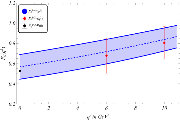
(a)

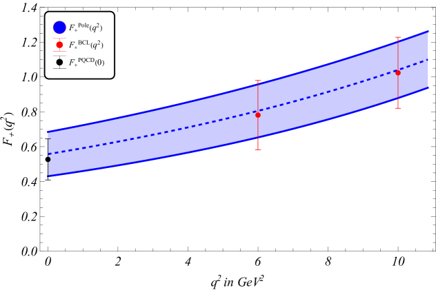
(b)

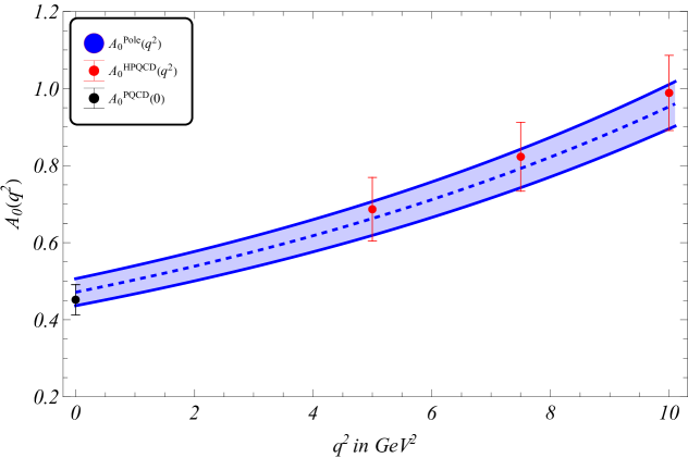
(c)

(d)

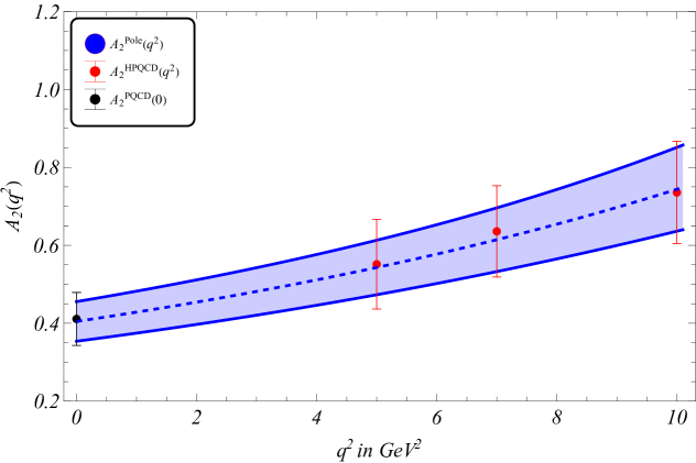
(e)

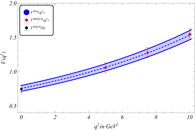
(f)

Figure 11: Plots showing the $q^{2}$ dependence of $B_{c}\rightarrow\eta_{c}$ and $B_{c}\rightarrow J/\psi$ semileptonic form factors. The blue curve denotes the distribution obtained using pole expansion parametrization, the red markers denote the synthetic data points from BCL and HPQCD, and the black marker is the pQCD value predicted in this work at $q^{2}=0.$

Appendix G $q^{2}$ distribution of $B_{c}\rightarrow P$ wave semileptonic decay widths:

In this appendix, we have discussed the $q^{2}$ distributions of the $B_{c}\to J/\psi$ and $B_{c}\to\eta_{c}$ form factors which we have obtained using the results of $q^{2}$ extrapolations parameters obtained in Table 11.

(a)

(b)

(c)

Figure 12: $q^{2}$ distribution of (a) $d\Gamma(B_{c}\rightarrow\chi_{c0})/dq^{2}$, (b) $d\Gamma(B_{c}\rightarrow\chi_{c1})/dq^{2}$ and (c) $d\Gamma(B_{c}\rightarrow h_{c})/dq^{2}$ semileptoic channels. The violet and green plots denote the light lepton and heavy lepton cases respectively.

References

- (1) “Hflav fit results as of moriond 2024.” https://hflav-eos.web.cern.ch/hflav-eos/semi/moriond24/html/RDsDsstar/RDRDs.html.
- (2) HFLAV collaboration, Averages of b-hadron, c-hadron, and -lepton properties as of 2021, Phys. Rev. D 107 (2023) 052008 [2206.07501].
- (3) I. Ray and S. Nandi, Test of new physics effects in decays with heavy and light leptons, JHEP 01 (2024) 022 [2305.11855].
- (4) LHCb collaboration, Measurement of the ratio of branching fractions /, Phys. Rev. Lett. 120 (2018) 121801 [1711.05623].
- (5) T.D. Cohen, H. Lamm and R.F. Lebed, Precision Model-Independent Bounds from Global Analysis of Form Factors, Phys. Rev. D 100 (2019) 094503 [1909.10691].
- (6) HPQCD collaboration, form factors for the full range from lattice QCD, Phys. Rev. D 102 (2020) 094518 [2007.06957].
- (7) LATTICE-HPQCD collaboration, and Lepton Flavor Universality Violating Observables from Lattice QCD, Phys. Rev. Lett. 125 (2020) 222003 [2007.06956].
- (8) A.Y. Anisimov, I.M. Narodetsky, C. Semay and B. Silvestre-Brac, The meson lifetime in the light front constituent quark model, Phys. Lett. B 452 (1999) 129 [hep-ph/9812514].
- (9) V.V. Kiselev, Exclusive decays and lifetime of meson in QCD sum rules, hep-ph/0211021.
- (10) M.A. Ivanov, J.G. Korner and P. Santorelli, Exclusive semileptonic and nonleptonic decays of the meson, Phys. Rev. D 73 (2006) 054024 [hep-ph/0602050].
- (11) E. Hernandez, J. Nieves and J.M. Verde-Velasco, Study of exclusive semileptonic and non-leptonic decays of - in a nonrelativistic quark model, Phys. Rev. D 74 (2006) 074008 [hep-ph/0607150].
- (12) W.-F. Wang, Y.-Y. Fan and Z.-J. Xiao, Semileptonic decays in the perturbative QCD approach, Chin. Phys. C 37 (2013) 093102 [1212.5903].
- (13) Z. Rui, Probing the -wave charmonium decays of meson, Phys. Rev. D 97 (2018) 033001 [1712.08928].
- (14) Z. Rui, J. Zhang and L.-L. Zhang, Semileptonic decays of meson to -wave charmonium states, Phys. Rev. D 98 (2018) 033007 [1806.00796].
- (15) X. Liu, H.-n. Li and Z.-J. Xiao, Improved perturbative qcd formalism for meson decays, Phys. Rev. D 97 (2018) 113001.
- (16) X.-Q. Hu, S.-P. Jin and Z.-J. Xiao, Semileptonic decays in the PQCD approach with the lattice QCD input, Chin. Phys. C 44 (2020) 053102 [1912.03981].
- (17) A. Biswas, S. Nandi and S. Sahoo, Analyzing the semileptonic and nonleptonic Bc → J/, c decays, JHEP 01 (2025) 198 [2311.00758].
- (18) M. Tanaka and R. Watanabe, Tau longitudinal polarization in B - D tau nu and its role in the search for charged Higgs boson, Phys. Rev. D 82 (2010) 034027 [1005.4306].
- (19) M. Tanaka and R. Watanabe, New physics in the weak interaction of , Phys. Rev. D 87 (2013) 034028 [1212.1878].
- (20) Y. Sakaki, M. Tanaka, A. Tayduganov and R. Watanabe, Testing leptoquark models in , Phys. Rev. D 88 (2013) 094012 [1309.0301].
- (21) H.-n. Li and H.-L. Yu, Perturbative QCD analysis of B meson decays, Phys. Rev. D 53 (1996) 2480 [hep-ph/9411308].
- (22) H.-N. Li and H.-L. Yu, PQCD analysis of exclusive charmless B meson decay spectra, Phys. Lett. B 353 (1995) 301.
- (23) H.-n. Li, PQCD analysis of exclusive B meson decays, in American Physical Society (APS) Meeting of the Division of Particles and Fields (DPF 99), 1, 1999 [hep-ph/9903323].
- (24) T. Kurimoto, H.-n. Li and A.I. Sanda, Leading power contributions to B — pi, rho transition form-factors, Phys. Rev. D 65 (2002) 014007 [hep-ph/0105003].
- (25) M. Nagashima and H.-n. Li, factorization of exclusive processes, Phys. Rev. D 67 (2003) 034001.
- (26) M. Nagashima and H.-n. Li, k(T) factorization of exclusive processes, Phys. Rev. D 67 (2003) 034001 [hep-ph/0210173].
- (27) T. Kurimoto, H.-n. Li and A.I. Sanda, B — D(*) form-factors in perturbative QCD, Phys. Rev. D 67 (2003) 054028 [hep-ph/0210289].
- (28) H.-n. Li, Threshold resummation for exclusive B meson decays, Phys. Rev. D 66 (2002) 094010 [hep-ph/0102013].
- (29) Z. Rui, H. Li, G.-x. Wang and Y. Xiao, Semileptonic decays of meson to S-wave charmonium states in the perturbative QCD approach, Eur. Phys. J. C 76 (2016) 564 [1602.08918].
- (30) H.-n. Li and B. Melic, Determination of heavy meson wave functions from B decays, Eur. Phys. J. C 11 (1999) 695 [hep-ph/9902205].
- (31) J.-F. Sun, D.-S. Du and Y.-L. Yang, Study of , decays with perturbative QCD approach, Eur. Phys. J. C 60 (2009) 107 [0808.3619].
- (32) S.J. Brodsky, T. Huang and G.P. Lepage, Hadronic and nuclear interactions in QCD, Springer Tracts Mod. Phys. 100 (1982) 81.
- (33) H.-Y. Cheng, C.-K. Chua and K.-C. Yang, Charmless hadronic B decays involving scalar mesons: Implications to the nature of light scalar mesons, Phys. Rev. D 73 (2006) 014017 [hep-ph/0508104].
- (34) C. McNeile, C.T.H. Davies, E. Follana, K. Hornbostel and G.P. Lepage, Heavy meson masses and decay constants from relativistic heavy quarks in full lattice QCD, Phys. Rev. D 86 (2012) 074503 [1207.0994].
- (35) D. Bečirević, G. Duplančić, B. Klajn, B. Melić and F. Sanfilippo, Lattice QCD and QCD sum rule determination of the decay constants of , J/ and states, Nucl. Phys. B 883 (2014) 306 [1312.2858].
- (36) G.C. Donald, C.T.H. Davies, R.J. Dowdall, E. Follana, K. Hornbostel, J. Koponen et al., Precision tests of the from full lattice QCD: mass, leptonic width and radiative decay rate to , Phys. Rev. D 86 (2012) 094501 [1208.2855].
- (37) HPQCD collaboration, decays from highly improved staggered quarks and NRQCD, PoS LATTICE2016 (2016) 281 [1611.01987].
- (38) E.E. Jenkins, M.E. Luke, A.V. Manohar and M.J. Savage, Semileptonic B(c) decay and heavy quark spin symmetry, Nucl. Phys. B 390 (1993) 463 [hep-ph/9204238].
- (39) Particle Data Group collaboration, Review of Particle Physics, PTEP 2022 (2022) 083C01.
- (40) Y. Li, M. Li and J.P. Vary, Two-photon transitions of charmonia on the light front, Phys. Rev. D 105 (2022) L071901 [2111.14178].
- (41) Belle collaboration, Search for resonant h Decays at Belle, Phys. Lett. B 662 (2008) 323 [hep-ex/0608037].
- (42) H.E. Martínez Neira, Phenomenology of the radiative E1 heavy quarkonium decay, Ph.D. thesis, Munich, Tech. U., 2017.
- (43) G.T. Bodwin and A. Petrelli, Order- corrections to -wave quarkonium decay, Phys. Rev. D 66 (2002) 094011 [hep-ph/0205210].
- (44) R. Zhu, Y. Ma, X.-L. Han and Z.-J. Xiao, Relativistic corrections to the form factors of into -wave Charmonium, Phys. Rev. D 95 (2017) 094012 [1703.03875].
- (45) H.S. Chung, P-wave quarkonium wavefunctions at the origin in the scheme, JHEP 09 (2021) 195 [2106.15514].
- (46) N. Kivel and M. Vanderhaeghen, Radiative decays within the QCD factorization framework, Phys. Rev. D 96 (2017) 054007 [1703.10383].
- (47) H.-K. Guo, Y.-Q. Ma and K.-T. Chao, Corrections to Hadronic and Electromagnetic Decays of Heavy Quarkonium, Phys. Rev. D 83 (2011) 114038 [1104.3138].
- (48) Z. Rui, J. Zhang and L.-l. Zhang, Semileptonic decays of meson to -wave charmonium states, Phys. Rev. D 98 (2018) 033007.
- (49) K. Azizi, H. Sundu and M. Bayar, Semileptonic B(c) to P-Wave Charmonia (X(c0), X(c1), h(c)) Transitions within QCD Sum Rules, Phys. Rev. D 79 (2009) 116001 [0902.1467].
- (50) X.-X. Wang, W. Wang and C.-D. Lu, B(c) to P-Wave Charmonia Transitions in Covariant Light-Front Approach, Phys. Rev. D 79 (2009) 114018 [0901.1934].
- (51) R. Zhu, Relativistic corrections to the form factors of into -wave orbitally excited charmonium, Nucl. Phys. B 931 (2018) 359 [1710.07011].
- (52) D. Melikhov and B. Stech, Weak form-factors for heavy meson decays: An Update, Phys. Rev. D 62 (2000) 014006 [hep-ph/0001113].
- (53) D. Leljak, B. Melic and M. Patra, On lepton flavour universality in semileptonic Bc → c, J/ decays, JHEP 05 (2019) 094 [1901.08368].
- (54) M.A. Ivanov, J.G. Korner and P. Santorelli, Semileptonic decays of mesons into charmonium states in a relativistic quark model, Phys. Rev. D 71 (2005) 094006 [hep-ph/0501051].
- (55) G. Buchalla, A.J. Buras and M.E. Lautenbacher, Weak decays beyond leading logarithms, Rev. Mod. Phys. 68 (1996) 1125 [hep-ph/9512380].
- (56) Z. Rui and Z.-T. Zou, S-wave ground state charmonium decays of mesons in the perturbative qcd approach, Phys. Rev. D 90 (2014) 114030.
- (57) C.-D. Lu, K. Ukai and M.-Z. Yang, Branching ratio and CP violation of B — pi pi decays in perturbative QCD approach, Phys. Rev. D 63 (2001) 074009 [hep-ph/0004213].
- (58) X. Liu, Z.-J. Xiao and C.-D. Lü, Pure annihilation type decays in the perturbative qcd approach, Phys. Rev. D 81 (2010) 014022.