An Efficient Learning Method to Connect Observables

Abstract

Constructing fast and accurate surrogate models is a key ingredient for making robust predictions in many topics. We introduce a new model, the Multiparameter Eigenvalue Problem (MEP) emulator. The new method connects emulators and can make predictions directly from observables to observables. We present that the MEP emulator can be trained with data from Eigenvector Continuation (EC) and Parametric Matrix Model (PMM) emulators. A simple simulation on a one-dimensional lattice confirms the performance of the MEP emulator. Using [28]O as an example, we also demonstrate that the predictive probability distribution of the target observables can be easily obtained through the new emulator.

A major theme in physics is to discover and understand phenomena. The gold standard for theoretical work is to explain experimental measurements and observations while also predicting unseen results. However, complexity in theory sometimes prevents all essential parameters from being uniquely determined. These parameters often appear in important constituents, such as a coupling strength in a Hamiltonian. Due to the variations of the parameters, calibrating the parameters and making a prediction often need to be done separately. These separate procedures work well when the underlying theory is simple enough and has only almost uniquely determined parameters. With the advance of physics, theoretical models tend to become complicated, ranging from cosmology models that have many parameters to be optimized [1, 2] to almost parameter-free theory of the underlying strong forces that is difficult to solve dynamically.

Low-energy nuclear physics lies in the intersection of computationally demanding and multiparametric. Delicate interplays of two- and three-body interactions have been one of the barriers to our theoretical progress, with many parameters called low-energy constants (LECs) appearing in the same order of the underlying effective field theory [3, 4, 5, 6]. These parameters cannot be directly measured, and the determination of LECs is already experiencing difficulties at the two-body level and needs a special strategy [7]. We have to remind ourselves that the non-observable LECs should serve as theoretical tools to simulate and bridge observables. As we know, some observables are strongly correlated, and it is interesting to look for a direct way to leverage the strong correlation, not in the context of LECs.

As a solution for the issue relevant to the universal physics problem, we propose a new explainable learning model named Multiparameter Eigenvalue Problem (MEP) emulator. Based on projection emulators in Refs. [8, 9, 10], the new method allows us to bypass parameter optimization steps and can construct a direct connection between calibrations and predictions. As illustrated in the flow chart Fig. 1, the MEP emulator can replace complicated statistical workflow found, for example, in Ref. [1, 2, 11, 12, 13]. We can directly obtain the conditional probability $P(\mathcal{O}_{\odot}|\{\mathcal{O}\})$ for the target $\mathcal{O}_{\odot}$ under the calibration data $\{\mathcal{O}\}$, once the probability density $P(\{\mathcal{O}\})$ of calibration observables is given, without going through the complicated workflow that is also dependent on the domain of parameters [13]. Our emulator has its root in the Ritz approximation method, enabling possible generalization to all problems that need multiple eigenvalues/parameters.

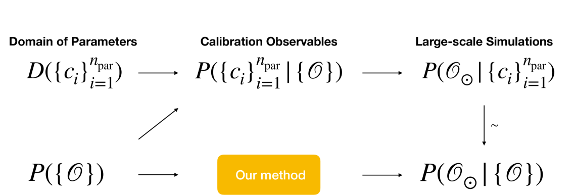
Figure 1: Workflow of our method compared with existing statistical procedures

We first briefly discuss our motivation. In many situations, we usually encounter the following Hamiltonian equation with the affine form:

$$\left(H_{0}+\sum_{i=1}^{n_{\rm par}}c_{i}H_{i}-EN\right)\mathbf{y}=0\,,$$ (1)

with a nontrivial vector $\mathbf{y}$. Here, $H_{0}$ is a parameter-free part of the Hamiltonian, $c_{i}$ is $i$-th parameter, $H_{i}$ is a part of the Hamiltonian depending on $c_{i}$, $E$ is the eigenvalue of the Hamiltonian, and $N$ is the norm kernel. A similar structure can be found in reduced order models such as EC methods [8], where the matrix elements of $H_{0}$, $H_{i}$, and $N$ are computed with the snapshot vectors. It is less discussed, but writing the equation in the above way, $E$ can be regarded as an input, as in scattering problems. Then, for example, $-c_{n_{\rm par}}$ can be regarded as the eigenvalue of the equation after multiplying the inverse $H^{-1}_{n_{\rm par}}$ (assuming it exists):

$$H_{n_{\rm par}}^{-1}\left(H_{0}+\sum_{i=1}^{n_{\rm par}-1}c_{i}H_{i}-EN\right)\mathbf{y}+c_{n_{\rm par}}\mathbf{y}=0\,.$$ (2)

This input-output exchange is a short and simple theoretical idea behind this work: we can make predictions without directly addressing the parameters in the Hamiltonian. We can further predict other quantities using $E$ as the input if only $c_{n_{\rm par}}$ is varied. Unfortunately, this is often not true. For example, in nucleon-nucleon interaction from chiral EFT in nuclear physics [4, 5], we generally expect that 10 - 30 parameters should be varied simultaneously to make meaningful predictions. Therefore, we would need to couple roughly the same number of Eq. (1). This number will continue to grow with our knowledge about three-nucleon interaction [14].

In the following, we consider the $m(>n_{\rm par})$ Hamiltonian equations that take $E^{[1]},\ldots,E^{[n_{\rm par}]}$ as inputs (to trade $n_{\rm par}$ parameters $c_{i}$) and $E^{[n_{\rm par}+1]},\ldots,E^{[m]}$ as outputs:

$$\left(H_{0}^{[j]}+\sum_{i=1}^{n_{\rm par}}c_{i}H_{i}^{[j]}-E^{[j]}N^{[j]}\right)\mathbf{y}^{[j]}=0\,,\leavevmode\nobreak\ \leavevmode\nobreak\ \leavevmode\nobreak\ 1\leq j\leq m\,.$$ (3)

Eq. (3) resembles the multiparameter eigenvalue problem (MEP) [15, 16], i.e.,

$$\left(O_{j}+\sum_{i=1}^{m}\alpha_{i}A_{ij}\right)\mathbf{y}_{j}=0\,,\leavevmode\nobreak\ \leavevmode\nobreak\ \leavevmode\nobreak\ 1\leq j\leq m\,.$$ (4)

Here, $O_{j}$ and $A_{ij}$ are square matrices, and $\alpha_{i}$ is a parameter of the generalized eigenvalue problem, hence it is referred to as a multiparameter eigenvalue. The solution is obtained by solving the generalized eigenvalue problem:

$$(K_{i}-\alpha_{i}K_{0})\mathbf{y}_{\otimes}=0\,,$$ (5)

with the generalized (Kronecker) determinants $K_{i}$ and $K_{0}$.

$$K_{i}=\begin{vmatrix}A_{11}&\cdots&A_{(i-1)1}&O_{1}&A_{{(i+1)1}}&\cdots&A_{m1}\\ \vdots&\vdots&\vdots&\vdots&\vdots&\vdots&\vdots\\ A_{1m}&\cdots&A_{(i-1)m}&O_{m}&A_{{(i+1)m}}&\cdots&A_{mm}\end{vmatrix}_{\otimes},$$ (6)

and

$$K_{0}=\begin{vmatrix}A_{11}&\cdots&A_{m1}\\ \vdots&\ddots&\vdots\\ A_{1m}&\cdots&A_{mm}\end{vmatrix}_{\otimes}.$$ (7)

The determinant is computed by replacing the matrix product with the Kronecker product, defined in Eq. (15) in Appendix . Different interpretations of Eq. (3) into Eq. (4) compose a superset of Hamiltonian multiparameter eigenvalue problems. For example, Eq. (3) can be found with $O_{j}=H_{0}^{[j]}+\sum_{i=1}^{n_{\rm par}}c_{i}H_{i}^{[j]}$, $A_{ij}=\delta_{ij}N^{[j]}$, and $\alpha_{i}=E^{[i]}$. This composes a set of decoupled MEP equations, i.e., $A_{ij}\propto\delta_{ij}$. Solving this system precisely corresponds to computing energy structures from a given parameter set $\{c_{i}\}_{i=1,\ldots,n_{\rm par}}$. On the other hand, when one requires to use $\{E^{[j]}\}_{j=1,\ldots,n_{\rm par}}$ as an input instead of $c_{i}$ to predict $\{E^{[j]}\}_{j=n_{\rm par}+1,\ldots,m}$, the following can be applied:

$$O_{j} =\left\{\begin{array}[]{rr}H_{0}^{[j]}-E^{[j]}N^{[j]}&1\leq j\leq n_{\rm par}\\ H_{0}^{[j]}&n_{\rm par}<j\leq m\end{array}\right.\,,$$ (8)

$$A_{ij} =\left\{\begin{array}[]{rr}H_{i}^{[j]}&1\leq j\leq n_{\rm par}\\ -\delta_{ij}N^{[i]}&n_{\rm par}<j\leq m\end{array}\right.\,,$$

$$\alpha_{i} =\left\{\begin{array}[]{rr}c_{i}&1\leq i\leq n_{\rm par}\\ E^{[i]}&n_{\rm par}<i\leq m\end{array}\right.\,.$$

With this rearrangement, $A_{ij}$ for $i\neq j$ does not vanish anymore, and the problem can be numerically expensive. Assuming that each equation in Eq. (4) has $M\times M$ dimension, the dimension of $K_{1}$ and $K_{i}$ is $M^{m}\times M^{m}$, and thus the size of the whole problem is not small as we have $m=10\sim 30$ in a typical nuclear physics application. The problems with such large dimension are unsolvable even on modern supercomputers. Even worse, we have not found a way to select the desired eigenvalue $E^{[j]}\,(n_{\rm par}<j\leq m)$ from the full set of $M^{m}$ eigenvalues. This point will be emphasized with a simple toy model, and a direct application of the known MEP to our problems is not suitable.

To overcome the issues, we consider a reduction of the problem size based on the idea of the projection emulator method. Suppose we have a set of $n_{\rm{train}}$ training parameters $S_{\rm{train}}=\{\mathbf{c}_{k}|\mathbf{c}_{k}=(c_{1,k},c_{2,k}\ldots,c_{n_{\rm{par}},k}),\;k=1,\ldots,n_{\rm{train}}\}$. Using the $k$-th training parameter set $\mathbf{c}_{k}$, we have an eigenvector $\mathbf{y}_{j,k}$ for the $j$-th equation in Eq. (4). The product of eigenvectors in Eq. (5) is then $\mathbf{y}_{\otimes,k}=\bigotimes_{j=1}^{m}\mathbf{y}_{j,k}$. The Kronecker determinant reduces to the usual matrix determinant after taking the inner product with $k$-th and $l$-th eigenvectors:

$$(\mathbf{y}_{\otimes,k})^{*}\cdot K_{0}\cdot\mathbf{y}_{\otimes,l}=\begin{vmatrix}(A_{11})_{kl}&\cdots&(A_{m1})_{kl}\\ \vdots&\ddots&\vdots\\ (A_{1m})_{kl}&\cdots&(A_{mm})_{kl}\end{vmatrix},$$ (9)

can be applied to any Kronecker determinants. Further details can be found in Appendix B. The object $(A_{ij})_{kl}\equiv(\mathbf{y}_{j,k})^{*}\cdot A_{ij}\cdot\mathbf{y}_{j,l}$, coincides with the $kl$-th element of subspace projected $A_{ij}$, and can be retrieved directly from original Hamiltonians. Once we know how to compute these inner products, we can explicitly write our MEP emulator for Eq. (5) from the subspace projection perspective. This projection works even if the Hamiltonian equations (3) are given by emulators. We denote the reduced order matrices for $K_{0}$ and $K_{i}$ by $\mathcal{K}_{0}$ and $\mathcal{K}_{i}$, with their $kl$-th entry computed from Eq. (9),

$$(\mathcal{K}_{i})_{kl} =(\mathbf{y}_{\otimes,k})^{*}\cdot K_{i}\cdot\mathbf{y}_{\otimes,l},$$ (10)

$$(\mathcal{K}_{0})_{kl} =(\mathbf{y}_{\otimes,k})^{*}\cdot K_{0}\cdot\mathbf{y}_{\otimes,l}.$$ (11)

Solving

$$(\mathcal{K}_{i}-\alpha_{i}\mathcal{K}_{0})\mathbf{y}=0,$$ (12)

will produce the desired eigenvalues/observables $\alpha_{i}$.

Besides the connection with the EC emulators, we notice that our reduced order model Eq. (12) preserves the nice affine form found in the original problem (3). Note that inputs of our MEP problem always enter the $O_{j}$ matrices, and they are on the same column in the determinant Eq. (6). Calculating the inner product Eq. (9) will always carry at maximum the same order of $\{E^{[j]}\}_{j=1,\ldots,n_{\rm par}}$ as it will appear in the original equation. Hence, we can always find

$$(\mathcal{K}_{i}-\alpha_{i}\mathcal{K}_{0})\mathbf{y}=(\mathcal{K}_{i0}+E^{[1]}\mathcal{K}_{i1}+\ldots\\ +E^{[n_{\rm par}]}\mathcal{K}_{in_{\rm par}}-\alpha_{i}\mathcal{K}_{0})\mathbf{y}=0\,.$$ (13)

This observation generalizes our application from EC to affine PMM emulators and can connect affine PMM and EC emulators. We shall focus on a demonstration of the MEP emulator in this work and defer the details of hybrid applications to the future.

(a)

(b)

Figure 2: The eigenvalue of the three-body system $E_{3}$ as a function of that of the two-body system $E_{2}$. The energies are computed with a simple Hamiltonian in the one-dimensional lattice, see text for the details. The training points for the EC emulator are represented by orange squares; blue dots represent validation from the original problem Eq. (3). In panel (a), the energies are computed by solving Eq. (5). The gray dots are obtained from the spectra of the original problem. Panel (b) shows the energies computed from the MEP emulator constructed with the ground-state eigenvectors. The solid (dashed) curve corresponds to ground-state $E_{2}$ and ground-state $E_{3}$ (excited-state $E_{2}$ and ground-state $E_{3}$). The triangles emphasize the corresponding $V_{0}$. The ground-state $E_{2}$ and $E_{3}$ as a function of $V_{0}$ are show in the top inset. The gray curve in the zoomed-in plot on the bottom is from inverting EC emulators according to Eq. (2).

Here, we show a proof-of-principle application of the MEP emulator with a simple one-dimensional lattice toy model based on the modified Generator code [17]. In the model, we set all the quantities as dimensionless and particle masses to be $m=1$, and the Hamiltonian is defined as $H=\sum_{i}^{N}T_{i}+\sum_{i<j}^{N}V_{ij}$ with the particle number $N$, one-body kinetic term $T_{i}$, and two-body interaction $V_{ij}$. The numerical calculations are performed within the space with lattice size $L=30$ and spacing $a_{\rm latt}=0.25$. For $T_{i}$, the $\mathcal{O}(a_{\text{latt}}^{3})$ improved lattice kinetic energy operator [18] is used. Also, the two-body contact interaction smeared with the Gaussian is employed; $V_{ij}=V_{0}\exp(-r_{ij}^{2}/R^{2})$, where $r_{ij}$ is the distance between the particles $i$ and $j$. Throughout this work, we use $R=2$. With this one-dimensional lattice model, we compute the ground states for $N=2$ and $3$ with various $V_{0}$ to investigate the performance of the MEP emulator. To do so, we first construct the EC emulators for two- and three-body systems with the computed snapshots at $V_{0}=0.5$, $-1$, $-2$, $-3$, $-4$, and $-5$.

In Figure 2a, we show the two- and three-body ground-state energies $E_{2}$ and $E_{3}$. Here, $E_{3}$ is obtained by solving the original MEP equation (5) as a function of $E_{2}$ instead of $V_{0}$. As seen in the figure, $M^{m}=36$ possible eigenvalues show complicated level crossings and branch switchings everywhere across the training domain. Moreover, the original lattice MEP equations have roughly $10^{6}$ eigenvalues in total. These crossings prevent a simple and general numerical scheme to extract the desired three-body ground-state energy for our problem. Furthermore, in EC emulators, training vectors usually are highly correlated, consequently, their normal matrices are not well-conditioned [9]. These not well-conditioned matrices hinder the accuracy of numerical operations in solving the MEP equations. We see many isolated dots in Fig. 2a that are obviously numerical artifacts. These two major issues forbid any meaningful interpretation of the results.

We proceed to check our MEP emulator (12) in Fig. 2b. The MEP emulator is constructed with the ground-state wave functions. With the $M\times M=6\times 6$ matrices, we can retrieve all our training data on the same branch (solid curve) that does not suffer from any switching. We also do not notice any numerical artifacts observed in Fig. 2a. With the MEP emulator, it is possible to select the ground-state $E_{3}$ by comparing $V_{0}$ computed from (12). At a fixed $E_{2}$, one can find different $V_{0}$ as shown by the triangles in the figure, and the branches indicated by the dashed curves correspond to excited-state $E_{2}$ obtained with a more attractive interaction. The strength $V_{0}$ can be efficiently retrieved because it shares the same eigenvector with the corresponding $E_{3}$. This scheme can be easily extended to general applications.

We also compare with the inversion Eq. (2), where the simple inversion is possible with a single varied parameter $V_{0}$. From the inset of the figure, we already notice a significant improvement in the scattering region. This is because the boundary condition heavily suppresses the $V_{0}$ dependence of discrete scattering eigenvalues [19]. Inverting this almost flat dependence will significantly amplify any numerical difference in Eq. (2) when emulating the energy levels. Only our new emulator can hold up in this simple toy test. We conclude that our MEP emulator is the only existing solution in some highly non-linear regions.

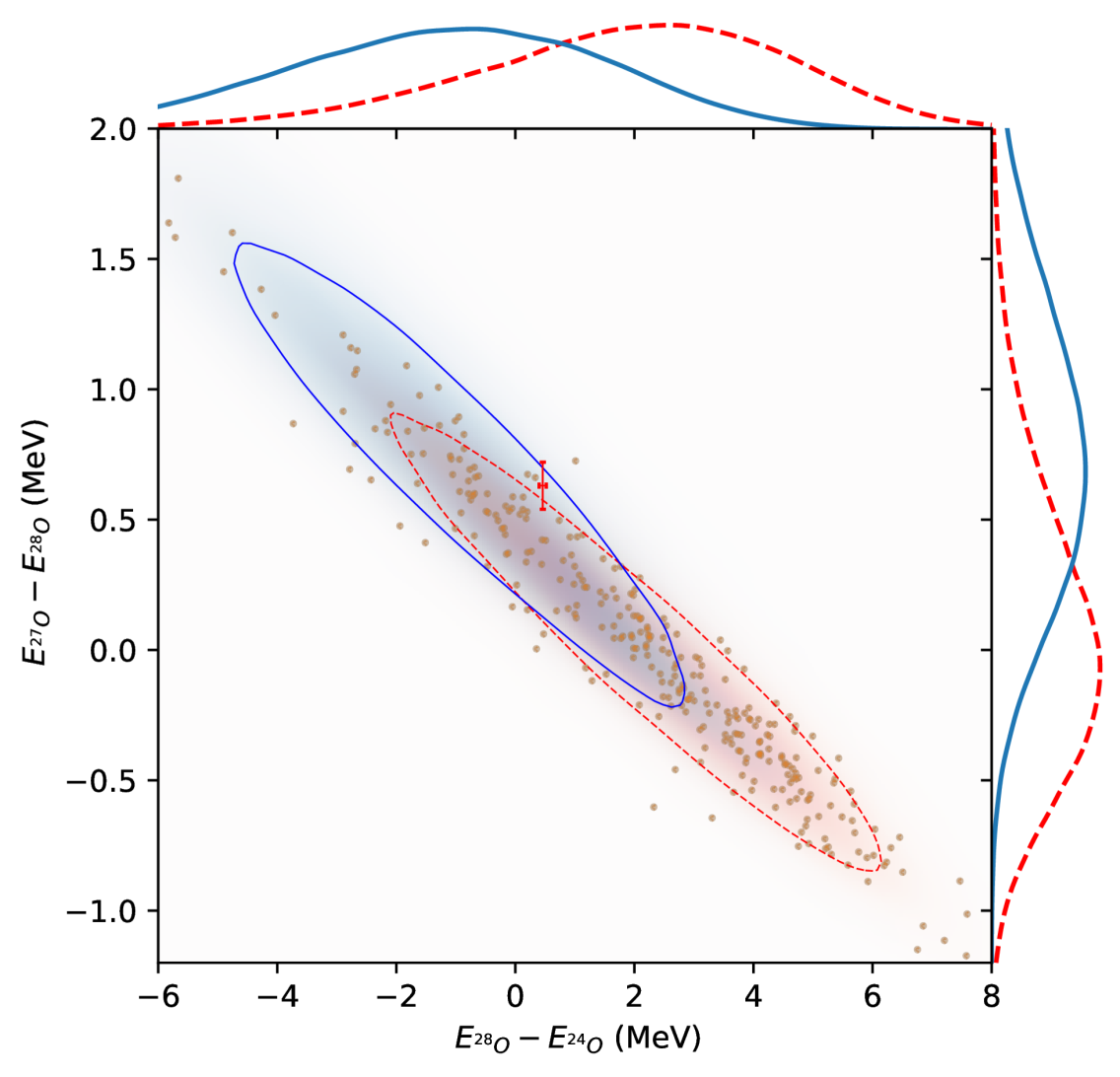
Figure 3: Joint probability density distributions of [28]O energy differences with respect to [27]O and [24]O. The red shade and red dashed lines are our emulator prediction using $10^{5}$ samples from averaging 10 bootstrapping batches with input constructed directly from $A=2-4$ NI measure [13]. The small orange dots are the data points used in constructing the emulators. We do not have any input from LECs. We then calibrate our joint density (blue shades and blue solid lines) with additional constraints on ground states of $A=16,24$ (see text). Circles are $1\sigma$ confident intervals (CIs). Red error bars are experimental values taken from Ref. [20].

For further validation, we consider a realistic problem from a data-driven aspect. In the following, we present the results using the valence-space in-medium similarity renormalization group (VS-IMSRG) [21, 22] to explore the energy of the newly discovered [28]O [20]. To this end, we numerically train the MEP emulator (13) using the PMM approach [10]. This approach allows us to directly find the matrices in Eq. (13) (see Appendix C for more details). We produce the training data using 300 non-implausible (NI) samples [13] of Delta-full chiral EFT interactions at the next-to-next-to-leading order [23] with momentum cutoff at $\Lambda=394$ MeV. The VS-IMSRG calculations are done within the 13 major-shell harmonic-oscillator (HO) space with the frequency parameter of $\hbar\omega=16$ MeV. Another truncation needs to be introduced for the three-nucleon matrix elements and is defined as $E_{\rm 3max}$ with the sum of the three-nucleon HO quanta. In this work, the sufficiently large $E_{\rm 3max}=18$ is used. With some calculations, we expect that the basis truncation error is around $0.2$ MeV for [24]O. We train two MEP emulators with the $12\times 12$ dimension matrices based on Eq. (13) using observable inputs to predict the ground-state energy differences of [27]O, [28]O and [28]O, [24]O. Our inputs include ground-state energies of [2]H, [3]H, [4]He, [6]Li, [16]O and [24]O, as well as proton-neutron scattering phase shifts in the NI samples at lab energies $E=5,50$ MeV. To make our system not overdetermined, we remove one phase shift at $E=50$ MeV in ${}^{3}P_{2}$ channel so that the total number of input observables equals the number of LECs. We do not notice any differences in adding more (highly correlated) phase shifts and making this system overdetermined, while removing ground state energies often leads to failed training. Although the computational cost of the NN scattering phase shift is cheap, in this work, we extract the phase shifts through the PMM emulator, which can be found in Appendix A.

With the constructed emulator, we can explore the energy properties of [28]O based on a probability density of the input observables, as the diagonalization of $12\times 12$ matrices allows us to compute millions of samples in a few minutes. In Fig. 3, the resulting probability distributions are illustrated. We begin with the simple multivariate Gaussian distribution based on the equally weighted 8188 NI sample data from Ref. [13]. Although this simple distribution does not properly include the theoretical uncertainties due to EFT and many-body truncations, etc., the obtained probability distribution (the dashed line in the figure) should somewhat show us an NI range of the target observables. Ref. [20] uses $A=16-24$ observables as calibration observables in their coupled-cluster calculations. To explore the impact of the calibration, we generate our calibrated distribution through the simple conditional Gaussian with marginal distributions centered at the experimental values of $E_{\isotope[16]{O}}=-127\pm 2$ MeV and $E_{\isotope[24]{O}}=-168\pm 3$ MeV. Note that standard deviations are ad hoc estimations based on model uncertainties [20] We generate these conditional samples as our new input. The corresponding probability distribution is given by the solid line in the figure. Compared with the literature [20], the results before the calibration are already consistent with experimental results, with our 68% CI region overlapping with the experimental CI region. After the calibration, it is observed that the predictive probability density moves closer to the experimental value, and the new 68% CI region overlaps with the experimental CI better. Again, the probability distributions discussed here do not include properly estimated uncertainties. However, once the proper uncertainties and input density are given, the same procedure can be easily applied, and one can obtain a more meaningful result. This example shows that our MEP emulator can be used to efficiently explore constraints given by observables and produce consistent predictions.

We introduce a novel deterministic emulator from the theory of the multiparameter eigenvalue problem to connect different model predictions – the MEP emulator. This new emulator is applicable to both model- and data-driven approaches. It is observed that the direct application of the multiparameter eigenvalue problem to a nuclear physics study is impossible without reduced basis methods. From the model-driven perspective, we thoroughly benchmark our MEP emulator and show its advantage in non-linear domains. As an application to a realistic problem, we discuss the probability distribution for the energy properties of the newly discovered [28]O. The MEP emulator allows us to simplify the workflow to understand and predict properties of atomic nuclei and to efficiently explore correlations between observables. Since the proposed procedure is general, one can expect potential adaptions to many different applications, including Multi-fidelity inputs [24], the volume-dependence perspective [19], and exploring time-dependent problems [16].

Appendix A Additoinal comments

For MEP, we note that $E^{[i]}$ in Eq. (3) is not necessarily an energy. A notable example is the phase shift. The most direct approach is to use the PMM. According to Ref. [10], this is always possible because the PMM can be a universal function approximator:

$$(H_{0}+c_{1}H_{1}+c_{2}H_{2}+\ldots+c_{n}H_{n}-\cot\delta_{l}I)\mathbf{y}=0\,.$$ (14)

The procedure has been numerically verified from training several PMM emulators for phase shift using the data from Ref. [13]. Eq. (14) can be added to Eq. (3), allowing us to use the phase shift as an additional input. Since we used the PMM method to numerically determine the affine matrices in Eq. (13), in this work, an explicit phase shift emulator construction is not necessary. We will discuss further details in a forthcoming publication.

Appendix B The inner product formula

Here, we derive the inner product in Eq. (9). Without losing generality, one can compute the inner product of $\mathbf{u}_{\otimes}^{*}\cdot K\cdot\mathbf{v}_{\otimes}$ in Eq. (5). The definition of the Kronecker determinant $K$ is

$$K=\begin{vmatrix}G_{11}&\cdots&G_{m1}\\ \vdots&\ddots&\vdots\\ G_{1m}&\cdots&G_{mm}\end{vmatrix}_{\otimes}\\ =\sum_{\sigma\in{S_{m}}}{\mathrm{sgn}(\sigma)}G_{\sigma(1)1}\otimes G_{\sigma(2)2}\ldots\otimes G_{\sigma(m)m}\\ \equiv\sum_{\sigma\in{S_{m}}}{\mathrm{sgn}(\sigma)}K_{\sigma}\,.$$ (15)

Then, we can write

$$\mathbf{u}_{\otimes}^{*}\cdot K\cdot\mathbf{v}_{\otimes}=\sum_{\sigma\in{S_{m}}}{\mathrm{sgn}(\sigma)}\mathbf{u}_{\otimes}^{*}K_{\sigma}\mathbf{v}_{\otimes}\,.$$ (16)

$\mathbf{u}_{\otimes}$ and $\mathbf{v}_{\otimes}$ are vectors belonging to the vector space of the corresponding linear operator $K$. Therefore, we can write

$$\mathbf{u}_{\otimes}=\mathbf{u}_{1}\otimes\mathbf{u}_{2}\otimes\ldots\otimes\mathbf{u}_{m}\,,\,$$ (17)

and

$$\mathbf{v}_{\otimes}=\mathbf{v}_{1}\otimes\mathbf{v}_{2}\otimes\ldots\otimes\mathbf{v}_{m}\,.$$ (18)

Then, the product can be written as

$$\mathbf{u}_{\otimes}^{*}\cdot K_{\sigma}\cdot\mathbf{v}_{\otimes}=(\mathbf{u}_{1}^{*}\otimes\mathbf{u}_{2}^{*}\otimes\ldots\otimes\mathbf{u}_{m}^{*})\cdot\\ (G_{\sigma(1)1}\otimes G_{\sigma(2)2}\otimes\ldots\otimes G_{\sigma(m)m})\cdot\\ (\mathbf{v}_{1}\otimes\mathbf{v}_{2}\otimes\ldots\otimes\mathbf{v}_{m}).$$ (19)

As the Kronecker product satisfies $(A\otimes B)\cdot(C\otimes D)\cdot(E\otimes F)=[(AC)\otimes(BD)]\cdot(E\otimes F)=(ACE)\otimes(BDF)$, one can find

$$\mathbf{u}_{\otimes}^{*}\cdot K_{\sigma}\cdot\mathbf{v}_{\otimes}=(\mathbf{u}_{1}^{*}G_{\sigma(1)1}\mathbf{v}_{1})\otimes\ldots\otimes(\mathbf{u}_{m}^{*}G_{\sigma(m)m}\mathbf{v}_{m})$$ (20)

The product $\mathbf{u}_{i}^{*}G_{i\sigma(i)}\mathbf{v}_{i}$ becomes a scalar, and thus

$$\mathbf{u}_{\otimes}^{*}\cdot K_{\sigma}\cdot\mathbf{v}_{\otimes}=\\ (\mathbf{u}_{1}^{*}G_{\sigma(1)1}\mathbf{v}_{1})\ldots(\mathbf{u}_{m}^{*}G_{\sigma(m)m}\mathbf{v}_{m})$$ (21)

is also a scalar. Substituting the result for Eq. (15), we obtain

$$\mathbf{u}_{\otimes}^{*}\cdot K\cdot\mathbf{v}_{\otimes}=\sum_{\sigma\in{S_{m}}}{\mathrm{sgn}(\sigma)}\\ \cdot(\mathbf{u}_{1}^{*}G_{\sigma(1)1}\mathbf{v}_{1})\cdot(\mathbf{u}_{2}^{*}G_{\sigma(2)2}\mathbf{v}_{2})\ldots\cdot(\mathbf{u}_{m}^{*}G_{\sigma(m)m}\mathbf{v}_{m}),$$ (22)

which coincides with the definition of the matrix determinant:

$$\mathbf{u}_{\otimes}^{*}\cdot K\cdot\mathbf{v}_{\otimes}=\begin{vmatrix}u_{1}^{*}G_{11}v_{1}&\cdots&u_{1}^{*}G_{m1}v_{1}\\ \vdots&\ddots&\vdots\\ u_{m}^{*}G_{1m}v_{m}&\cdots&u_{m}^{*}G_{mm}v_{m}\end{vmatrix}.$$ (23)

Appendix C PMM for VS-IMSRG

The VS-IMSRG has been one of the very successful many-body techniques in nuclear theory. To make a robust prediction through the VS-IMSRG calculations, one would need to run the million or billion times calculation, which is clearly unrealistic. Therefore, the construction of a fast and accurate VS-IMSRG emulator is an essential task. The widely applied EC method, however, does not allow us to construct the emulator, as access to the VS-IMSRG eigenvector is not straightforward. Parametric Matrix Model (PMM) is a class of newly developed model- and data-driven hybrid emulators [10]. In contrast to the EC method, the PMM needs only the eigenvalues, making the emulator construction feasible. We have observed that the PMM often performed better than more general data-driven models, including the Gaussian Process on smaller datasets [25].

We briefly discuss PMM for the VS-IMSRG and validate its performance. For emulators built directly from LECs input $c_{i}$, we solve the following equation:

$$(H_{0}+c_{1}H_{1}+c_{2}H_{2}+\ldots+c_{n}H_{n}-EI)\mathbf{y}=0\,,$$ (24)

It is almost the replication of Eq. (1), with the choice of norm kernels to be always $I$. The matrix elements of $H_{i}$ are acquired by a machine learning method that minimizes a loss function with the predictions in the following steps: First, we generate random hermitian $H_{i}$. Then we compute the (usually lowest) eigenvalue of Eq. (24) $E_{\rm PMM}$ with a given training set $\{c_{i}\}$. The difference between training target $E$ and $E_{\rm PMM}$ will enter the loss function. Finally, we use (Adam [26]) gradient descent on the $H_{i}$ elements to optimize the loss function, hence the name “Parametric Matrix”. In our case, we choose the simple mean absolute loss function $l_{\rm{MAE}}$ that averages the absolute difference between the PMM and VS-IMSRG results:

$$l_{\rm{MAE}}[\{H_{i}\}_{i=0,\ldots,n}]=\frac{1}{N_{\rm train}}\sum_{k=1}^{N_{\rm train}}|E_{k}-E_{k,{\rm PMM}}|\,.$$ (25)

For the NI samples, we estimate the required number of training samples $N_{\rm train}$ with the [16]O data. We observed that $N_{\rm train}=300-500$ with $12\times 12$ PMM matrix size provides the accurate results for the total 8188 NI samples with the mean absolute error of 0.1 MeV, which is smaller than the other theoretical uncertainties [11, 20]

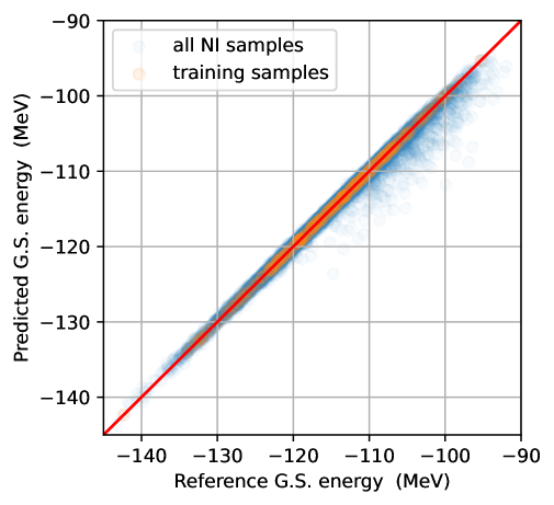
(a) PMM emulator for ¹⁶O

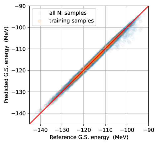
(b) MEP emulator for ¹⁶O

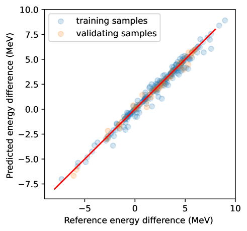
(c) MEP emulator for $E_{\isotope[28]{O}}-E_{\isotope[24]{O}}$

Figure 4: Performance of emulators. Panels (a) and (b) show the performance for the ground-state energy for [16]O, where the emulators take the 17 LECs and observables as inputs, respectively. Panel (c) is for the MEP emulator targeting the ground-state energy difference between [24]O and [28]O. The training and validation data are given with the orange and blue circles, respectively.

With the 8188 NI samples available, we use the ground-state energy of [16]O to test the performance of the PMM and MEP emulators for the VS-IMSRG calculations. As illustrated in Fig. 4a, it is seen that the PMM emulator with the 17 active LECs trained with the randomly selected 300 NI samples works well. Similarly, Fig. 4b demonstrates a good performance of the MEP emulator, trained with the 17 input observables, i.e., the NN scattering phase shifts and ground-state energies of the few-body systems.

As one can easily find that the affine form is preserved for an energy difference in the MEP emulator, we can take $E_{\isotope[24]{O}}-E_{\isotope[28]{O}}$ as our output:

$$\Big{[}\mathcal{K}_{i0}+E^{[1]}\mathcal{K}_{i1}+\ldots+E^{[n-1]}\mathcal{K}_{i(n-1)}+E_{\isotope[24]{O}}(\mathcal{K}_{in}-\mathcal{K}_{0})\\ +(E_{\isotope[24]{O}}-E_{\isotope[28]{O}})\mathcal{K}_{0}\Big{]}\mathbf{y}=0.$$ (26)

Eq. (26) allows us to emulate a differential quantity directly, which incorporates a cancellation of the systematic uncertainty of the theoretical calculations. We then present our final validation in Fig. 4c. This is a pure MEP prediction with training data generated from the VS-IMSRG calculations described in the main text. Starting from the available 300 VS-IMSRG results, we perform a bootstrapping analysis to test the general performance of our method. We randomly choose a subset of 250 data points from the 300 samples. Then, for each bootstrapping batch, we take 240 random resamples from this subset and train a new MEP emulator. The whole training takes roughly 10 minutes for 100 batches on a laptop computer. The averages of these 100 emulators and predictions on the remaining 50 data points are displayed in Fig. 4c. With this validation, we find the mean absolute error from our bootstrapping to be 0.2 MeV. This would be acceptable in the current application because the basis truncation error is larger, i.e., the energy difference between $e_{\rm max}=12$ and $16$ results is about $0.6$ MeV for [28]O. This bias will shift $E_{\isotope[27]{O}}-E_{\isotope[28]{O}}$ by $+0.2$ MeV. Basis truncation errors are closely related to the continuum effect [19]. The previous estimation of the effect on energy differences $E_{\isotope[28]{O}}-E_{\isotope[24]{O}}$ owing to continuum is around 1 MeV [27]. Including these continuum effects and basis truncation errors in the VS-IMSRG is beyond the scope of this work.

References

- Bower et al. [2010] R. G. Bower, M. Goldstein, and I. Vernon, Galaxy formation: a Bayesian uncertainty analysis, Bayesian Analysis 5, 619 (2010).
- Vernon et al. [2014] I. Vernon, M. Goldstein, and R. Bower, Galaxy formation: Bayesian history matching for the observable universe, Statistical science , 81 (2014).
- Weinberg [1979] S. Weinberg, Phenomenological Lagrangians, Physica A 96, 327 (1979).
- Epelbaum et al. [2009] E. Epelbaum, H.-W. Hammer, and U.-G. Meissner, Modern Theory of Nuclear Forces, Rev. Mod. Phys. 81, 1773 (2009), arXiv:0811.1338 [nucl-th] .
- Machleidt and Entem [2011] R. Machleidt and D. R. Entem, Chiral effective field theory and nuclear forces, Phys. Rept. 503, 1 (2011), arXiv:1105.2919 [nucl-th] .
- Hammer et al. [2020] H. W. Hammer, S. König, and U. van Kolck, Nuclear effective field theory: status and perspectives, Rev. Mod. Phys. 92, 025004 (2020), arXiv:1906.12122 [nucl-th] .
- Peng et al. [2024] R. Peng, B. Long, and F.-R. Xu, Contact operators in renormalization of attractive singular potentials, Phys. Rev. C 110, 054001 (2024), arXiv:2407.08342 [nucl-th] .
- Frame et al. [2018] D. Frame, R. He, I. Ipsen, D. Lee, D. Lee, and E. Rrapaj, Eigenvector continuation with subspace learning, Phys. Rev. Lett. 121, 032501 (2018), arXiv:1711.07090 [nucl-th] .
- Duguet et al. [2024] T. Duguet, A. Ekström, R. J. Furnstahl, S. König, and D. Lee, Colloquium: Eigenvector continuation and projection-based emulators, Rev. Mod. Phys. 96, 031002 (2024), arXiv:2310.19419 [nucl-th] .
- Cook et al. [2024] P. Cook, D. Jammooa, M. Hjorth-Jensen, D. D. Lee, and D. Lee, Parametric Matrix Models (2024), arXiv:2401.11694 [cs.LG] .
- Hu et al. [2022] B. Hu et al., Ab initio predictions link the neutron skin of 208Pb to nuclear forces, Nature Phys. 18, 1196 (2022), arXiv:2112.01125 [nucl-th] .
- Elhatisari et al. [2024] S. Elhatisari et al., Wavefunction matching for solving quantum many-body problems, Nature 630, 59 (2024), arXiv:2210.17488 [nucl-th] .
- Jiang et al. [2024] W. G. Jiang, C. Forssén, T. Djärv, and G. Hagen, Emulating ab initio computations of infinite nucleonic matter, Phys. Rev. C 109, 064314 (2024), arXiv:2212.13216 [nucl-th] .
- Epelbaum et al. [2015] E. Epelbaum, A. M. Gasparyan, H. Krebs, and C. Schat, Three-nucleon force at large distances: Insights from chiral effective field theory and the large-Nc expansion, Eur. Phys. J. A 51, 26 (2015), arXiv:1411.3612 [nucl-th] .
- Atkinson [1968] F. V. Atkinson, Multiparameter spectral theory, Bulletin of the American Mathematical Society 74, 1 (1968).
- Atkinson and Mingarelli [2010] F. V. Atkinson and A. B. Mingarelli, Multiparameter eigenvalue problems: Sturm-Liouville theory (CRC Press, 2010).
- König and Lee [2018] S. König and D. Lee, Volume Dependence of N-Body Bound States, Phys. Lett. B 779, 9 (2018), arXiv:1701.00279 [hep-lat] .
- Lähde and Meißner [2019] T. A. Lähde and U.-G. Meißner, Nuclear Lattice Effective Field Theory: An introduction, Vol. 957 (Springer, 2019).
- Luscher [1991] M. Luscher, Two particle states on a torus and their relation to the scattering matrix, Nucl. Phys. B 354, 531 (1991).
- Kondo et al. [2023] Y. Kondo et al., First observation of 28O, Nature 620, 965 (2023), [Erratum: Nature 623, E13 (2023)].
- Stroberg et al. [2019] S. R. Stroberg, S. K. Bogner, H. Hergert, and J. D. Holt, Nonempirical Interactions for the Nuclear Shell Model: An Update, Ann. Rev. Nucl. Part. Sci. 69, 307 (2019), arXiv:1902.06154 [nucl-th] .
- Hergert [2020] H. Hergert, A Guided Tour of Nuclear Many-Body Theory, Front. in Phys. 8, 379 (2020), arXiv:2008.05061 [nucl-th] .
- Ekström et al. [2018] A. Ekström, G. Hagen, T. D. Morris, T. Papenbrock, and P. D. Schwartz, isobars and nuclear saturation, Phys. Rev. C 97, 024332 (2018), arXiv:1707.09028 [nucl-th] .
- Belley et al. [2024] A. Belley et al., Ab initio Uncertainty Quantification of Neutrinoless Double-Beta Decay in Ge76, Phys. Rev. Lett. 132, 182502 (2024), arXiv:2308.15634 [nucl-th] .
- Somasundaram et al. [2024] R. Somasundaram, C. L. Armstrong, P. Giuliani, K. Godbey, S. Gandolfi, and I. Tews, Emulators for scarce and noisy data: application to auxiliary field diffusion Monte Carlo for the deuteron (2024), arXiv:2404.11566 [nucl-th] .
- Kingma and Ba [2017] D. P. Kingma and J. Ba, Adam: A method for stochastic optimization (2017), arXiv:1412.6980 [cs.LG] .
- Hagen et al. [2016] G. Hagen, G. R. Jansen, M. Hjorth-Jensen, and T. Papenbrock, Emergent properties of nuclei from ab initio coupled-cluster calculations, Phys. Scripta 91, 063006 (2016), arXiv:1601.08203 [nucl-th] .