Nonuniform superconducting states caused by odd-frequency Cooper pairs

Abstract

We discuss the origin of a nonuniform superconducting state in which Cooper pairs have a finite center of mass momentum. The instability to such a nonuniform superconducting state is analyzed by a pole of the pair fluctuation propagator for weak coupling superconductors. The results show that odd(even)-frequency Cooper pairs stabilize a nonuniform (uniform) superconducting phase below the transition temperature. We provide a theoretical framework that explains the reasons for appearing the nonuniform superconducting states.

I Introduction

Fulde-Ferrell-Larkin-Ovchinnikov (FFLO) state is a possible superconducting state in a conventional superconductor (SC) under a Zeeman field [1, 2]. A Cooper pair has a finite center of mass momentum because Kramers partners no longer stay in the same energy level. As a result, the pair potential oscillates in real space. Such spatially nonuniform superconducting states are also feasible in the absence of Zeeman fields when electronic structures of a SC break time-reversal symmetry spontaneously [3, 4, 5]. Thus the time-reversal symmetry breaking (TRSB) fields have been considered as a source of the spatially nonuniform superconducting states. However, recent theoretical studies have indicated the possibility of nonuniform superconductivity in time-reversal symmetry preserving SCs such as a noncentrosymmetric SC and a $j=3/2$ SC [6, 7]. For example, the results in a $j=3/2$ SC suggest that interband Cooper pairs stabilize the nonuniform superconducting state. To our knowledge, however, interband Cooper pairs can form the uniform pair potentials in other cases [8]. A clearer and more comprehensive physical picture that explains a mechanism of stabilizing nonuniform superconducting states is desired. We address such an issue in the present paper.

To clarify the problem, we summarize our knowledge on inhomogeneous superconducting states near a vortex core [9], those near a magnetic impurity (cluster) [10, 11, 12, 13], and those at the surface of an anisotropic SC [14, 15]. These theoretical studies showed the existence of odd-frequency Cooper pairs [16, 17, 18, 19, 20, 21] in the inhomogeneous region. Odd-frequency Cooper pairs appear as an induced pairing correlation by these local defects. In bulk region, usual even-frequency Cooper pairs form the pair potentials and stabilize the superconducting states. The odd-frequency pairing correlation functions always constitute a part of the solution of the Eilenberger equation in inhomogeneous SCs [22] and make local superfluid density $n(\bm{r})$ negative due to their paramagnetic property [23, 24]. The spatial variation of the pair potential increase the energy of $\Delta E(\bm{r})\approx n(\bm{r})\,\bm{q}^{2}/m$ locally with $\bm{q}$ and $m$ being the momentum and the effective mass of a Cooper pair, respectively. When odd-frequency pairs reduce the superfluid density $n(\bm{r})$ locally, the energy cost decreases by such amount. Thus, the local deformation of the pair potential around the defect is supported by odd-frequency Cooper pairs appearing there. In what follows, we will show that this is also true for nonuniform superconducting states in the bulk. The existence of odd-frequency Cooper pairs in the bulk was first pointed out in uniform multiband/orbital SCs [25]. Odd-frequency pairs increase the free-energy and then decrease the transition temperature of uniform superconducting states because of their paramagnetic responce [26]. The conclusions in these studies suggest an important role of odd-frequency Cooper pairs in the transition from a uniform superconducting state to a nonuniform one.

The aim of the present paper is to provide a theoretical framework that explains the reasons for appearing the nonuniform superconducting states. To this end, we examine the instability of a normal state in the presence of attractive interaction between two electrons [27] by calculating the pair fluctuation propagator $D_{q}$ within the ladder approximation [28]. We compare two transition temperatures. One is the transition temperature to a uniform superconducting state $T_{\bm{0}}$. The other is the transition temperature to a nonuniform superconducting state $T_{\bm{q}}$ in which Cooper pairs have a finite center of mass momentum $\bm{q}$. The transition temperatures are determined by the pole of the pair fluctuations propagator $D_{q}^{-1}\propto a+Bq^{2}=0$. For $B>0$, $T_{\bm{0}}$ determined by $a=0$ at $q=0$ is always larger than $T_{\bm{q}}$, which indicates the transition to a uniform state. On the other hand, we find $T_{\bm{q}}>T_{\bm{0}}$ is satisfied for $B<0$, which means the appearance of a nonuniform state. We confirm that this theoretical framework successfully describes the appearance of already known nonuniform superconducting state such as FFLO state in a spin-singlet $s$-wave SC in a Zeeman field. Most importantly, we find that the coefficient $B$ is proportional to the Meissner kernel or the superfluid density in a uniform superconducting state. Namely, odd-frequency Cooper pairs decrease the superfluid density to be negative in a uniform superconducting state. This fact explains the reason for the appearance of a nonuniform superconducting state.

We also find stable nonuniform superconducting states in a two-band SC with $s$-wave interband pairing order [29] and in a $j=3/2$ SC with $s$-wave pseudospin-quintet pairing order [30]. The band hybridization (and/or the asymmetry between the two bands) and the spin-orbit interaction generate odd-frequency Cooper pairs in a two-band SC and a $j=3/2$ SC, respectively. By solving $D_{q}^{-1}=0$ numerically, we will show that a nonuniform superconducting state becomes more stable than a uniform one in these time-reversal symmetry preserving SCs. We also find in a single-band SC that any perturbations generating odd-frequency Cooper pairs break time-reversal symmetry. We conclude that odd-frequency Cooper pairs support the transition to the nonuniform superconducting states.

The paper is organized as follows. In Sec. II, we derive the analytic expression of the pair fluctuation propagator for a weak coupling SC. We also discuss the relationship between the frequency symmetry of Cooper pairs in a uniform phase and stability of the nonuniform phase. In Sec. III, we revisit the transition to the FFLO state in a conventional spin-singlet $s$-wave SC under Zeeman fields. We reinterpret the FFLO state in terms of the subdominant odd-frequency pairing correlation. In Sec. IV, we demonstrate the appearance of a nonuniform superconducting phase in time-reversal symmetry preserving SCs such as a two-band SC and a $j=3/2$ SC. The role of symmetry-breaking perturbations such as Zeeman fields and relating phenomena to our results are discussed in Sec. V. The conclusions are given in Sec. VI. Throughout this paper, we use the units of $k_{\mathrm{B}}=c=\hbar=1$ where $k_{\mathrm{B}}$ is the Boltzmann constant and $c$ is the speed of light and $e<0$ is charge of an electron.

II Pair fluctuation propagator

In this paper, we analyze the following Hamiltonian describing the electronic states with effective electron-electron interaction:

$$\mathcal{H} =\mathcal{H}_{0}+\mathcal{H}_{1},$$ (1)

$$\mathcal{H}_{0} =\sum_{\bm{k}\alpha\beta}\xi_{\bm{k}\alpha\beta}c^{{\dagger}}_{\bm{k}\alpha}c_{\bm{k}\beta},\quad\xi_{\bm{k}\alpha\beta}=\epsilon_{\bm{k}\alpha\beta}-\mu\delta_{\alpha\beta},$$ (2)

$$\mathcal{H}_{1} =-g\sum_{\bm{q}}\Phi^{{\dagger}}_{\bm{q}}\Phi_{\bm{q}},$$ (3)

$$\Phi_{\bm{q}} =\frac{1}{\sqrt{2N}}\sum_{\bm{k}^{\prime}\gamma\delta}w^{\ast}_{\gamma\delta}(\bm{k}^{\prime})c_{\bm{k}^{\prime}+\frac{\bm{q}}{2}\gamma}c_{-\bm{k}^{\prime}+\frac{\bm{q}}{2}\delta},$$ (4)

where $\alpha,\beta,\gamma,\delta$ represent the internal degree of freedom of an electron such as spin, band, orbital, and sublattice, etc, $c_{\bm{k}\alpha}$ is the annihilation operator of an electron at $\bm{k}$ with $\alpha$, and $g>0$ represents the strength of the attractive interaction. $\Phi_{\bm{q}}$ is the annihilation operator of a Cooper pair with the center of mass momentum $\bm{q}$, and $N$ is the number of unit cells of the underlying lattice. The attractive interaction is characterized by $w_{\sigma\sigma^{\prime}}(\bm{k})$, which satisfies $w_{\sigma\sigma^{\prime}}(\bm{k})=-w_{\sigma^{\prime}\sigma}(-\bm{k})$ due to the fermion anticommutation relation.

Within the linear response theory [28], the transition from a normal state to a superconducting state is examined by analyzing the pole of the pair fluctuation propagator which is defined by

$$D_{\mathrm{s}}(\bm{q},i\nu_{n}) \coloneqq-\int_{0}^{1/T}d\tau\,\langle T_{\tau}\Phi_{\bm{q}}(\tau)\Phi^{{\dagger}}_{\bm{q}}\rangle\,e^{i\nu_{n}\tau},$$ (5)

where $\nu_{n}=2n\pi T$ is the bosonic Matsubara frequency with $n$ being an integer and $T$ being the temperature, and $\Phi_{\bm{q}}(\tau)=e^{\tau\mathcal{H}}\Phi_{\bm{q}}e^{-\tau\mathcal{H}}$. By summing the ladder diagrams, we obtain

$$D_{\mathrm{s}}(\bm{q},i\nu_{n}) =\frac{-\Pi_{\mathrm{s}0}(\bm{q},i\nu_{n})}{1-g\Pi_{\mathrm{s}0}(\bm{q},i\nu_{n})},$$ (6)

$$\Pi_{\mathrm{s}0}(\bm{q},i\nu_{n}) =-T\sum_{\omega_{\ell}}\frac{1}{N}\sum_{\bm{k}}\mathrm{Tr}\left[\hat{\mathcal{G}}_{0}(\bm{k}+\bm{q}/2,i\omega_{\ell})\hat{w}(\bm{k})\right.$$

$$\left.\hskip 30.00005pt\times\hat{\underline{\mathcal{G}}}_{0}(\bm{k}-\bm{q}/2,i\omega_{\ell}-i\nu_{n})\hat{w}^{{\dagger}}(\bm{k})\right],$$ (7)

where $\hat{\mathcal{G}}_{0}(\bm{k},i\omega_{\ell})=[i\omega_{\ell}-\hat{\xi}_{\bm{k}}]^{-1}$ is the Green’s function in the absence of the attractive interaction, $\underline{X}(\bm{k},i\omega_{\ell})\coloneqq-X^{\ast}(-\bm{k},i\omega_{\ell})$ represents particle-hole conjugation of a function $X(\bm{k},i\omega_{\ell})$ and $\omega_{\ell}=(2\ell+1)\pi T$ is the fermionic Matsubara frequency with $\ell$ being an integer. The second-order transition to a superconducting phase is characterized by the divergence of the retarded propagator $D^{\mathrm{R}}_{\mathrm{s}}(\bm{q},\omega)\coloneqq D_{\mathrm{s}}(\bm{q},i\nu_{n}\rightarrow\omega+i\delta)$. In the following, we put $\omega=0$ as we focus on static superconducting states. To discuss the transition to nonuniform superconducting states, we expand the pair polarization function $\Pi^{\mathrm{R}}_{\mathrm{s}0}(\bm{q},0)\coloneqq\Pi_{\mathrm{s}0}(\bm{q},i\nu_{n}\rightarrow\omega+i\delta=0)$ with respect to $\bm{q}$:

$$\Pi^{\mathrm{R}}_{\mathrm{s}0}(\bm{q},0) =-T\sum_{\omega_{\ell}}\frac{1}{N}\sum_{\bm{k}}\mathrm{Tr}\left[\hat{\mathcal{G}}_{0}\hat{w}\hat{\mathcal{\underline{G}}}_{0}\hat{\underline{w}}\right.$$

$$\left.-\frac{q_{\mu}q_{\nu}}{4}\mathrm{Re}\left[\partial_{k_{\mu}}\partial_{k_{\nu}}\hat{\xi}\hat{\mathcal{G}}_{0}\hat{w}\hat{\mathcal{\underline{G}}}_{0}\hat{\underline{w}}\hat{\mathcal{G}}_{0}+\hat{v}_{\mu}\hat{\mathcal{G}}_{0}\hat{v}_{\nu}\hat{\mathcal{G}}_{0}\hat{w}\hat{\mathcal{\underline{G}}}_{0}\hat{\underline{w}}\hat{\mathcal{G}}_{0}\hat{v}_{\mu}\hat{\mathcal{G}}_{0}\hat{w}\hat{\mathcal{\underline{G}}}_{0}\hat{\underline{w}}\hat{\mathcal{G}}_{0}\hat{v}_{\nu}\hat{\mathcal{G}}_{0}+\hat{v}_{\mu}\hat{\mathcal{G}}_{0}\hat{w}\hat{\mathcal{\underline{G}}}_{0}\hat{\underline{v}}_{\nu}\hat{\mathcal{\underline{G}}}_{0}\hat{\underline{w}}\hat{\mathcal{G}}_{0}\right]+O(q^{4})\right],$$ (8)

where the sum of the repeated indices for $\mu,\nu=x,y,z$ are taken, $\partial_{k_{\mu}}fg=\frac{\partial f}{\partial k_{\mu}}g$, $\hat{v}_{\mu}\coloneqq\partial_{k_{\mu}}\hat{\xi}$ is the velocity operator, and $\hat{\mathcal{G}}_{0}$, $\hat{w}$, $\hat{\underline{w}}$, and $\hat{\underline{v}}_{\mu}$ are the abbreviation of $\hat{\mathcal{G}}_{0}(\bm{k},i\omega_{\ell})$, $\hat{w}(\bm{k})$, $-\hat{w}^{\ast}(-\bm{k})$, and $-\hat{v}^{\ast}_{\mu}(-\bm{k})$, respectively. In Eq. (8), we assumed the odd orders with respect to $\bm{q}$ vanish for simplicity .

We find that the pair fluctuation propagator is expressed by using the Meissner kernel in the uniform superconducting order:

$$\left[D^{\mathrm{R}}_{\mathrm{s}}(\bm{q},0)\right]^{-1} \propto a(T)+B_{\mu\nu}(T)q_{\mu}q_{\nu}+O(q^{4}),$$ (9)

$$a(T) =\frac{1}{g}+T\sum_{\omega_{\ell}}\frac{1}{N}\sum_{\bm{k}}\mathrm{Tr}\left[\hat{\mathcal{G}}_{0}\hat{w}\hat{\mathcal{\underline{G}}}_{0}\hat{\underline{w}}\right],$$ (10)

$$B_{\mu\nu}(T) =\left.\frac{K_{\mu\nu}(\bm{0},0)}{4e^{2}\alpha^{2}|\Delta^{2}|}\right|_{\Delta=0},$$ (11)

where $a(T)$ and $K_{\mu\nu}(\bm{0},0)$ correspond to a quadratic coefficient of the Ginzburg-Landau (GL) free-energy and the Meissner kernel for a uniform superconducting state, respectively. The derivation of the Meissner kernel is presented in Appendix. A. In Eq. (11), constants $\alpha\in\mathbb{R}$ and $\Delta\in\mathbb{C}$ satisfies the relation $\hat{\Delta}(\bm{k})=\alpha\Delta\hat{w}(\bm{k})$, where $\hat{\Delta}(\bm{k})$ is the pair potential entering the Bogoliubov-de Gennes (BdG) Hamiltonian of the uniform state, which is defined in Eq. (92). Without loss of generality, the GL free-energy of a uniform superconducting state can be given by

$$\Omega_{\mathrm{GL}}(\Delta)=a(T)\,|\Delta|^{2}+b(T)\,|\Delta|^{4}+O(\Delta^{6}).$$ (12)

The transition temperature to a uniform superconducting state $T_{\bm{0}}$ is defined by

$$a(T_{\bm{0}})=0,$$ (13)

because $a(T)$ changes the sign at $T=T_{\bm{0}}$. $b>0$ grantees the second order transition (continuous transition) to the superconducting state. On the other hand, $b<0$ indicates that the transition to the uniform superconducting state becomes discontinuous.

Using Eq. (9), the transition temperature to nonuniform superconducting state $T_{\bm{q}}$ is defined by

$$a(T_{\bm{q}})+B_{\mu\nu}(T_{\bm{q}})q_{\mu}\,q_{\nu}=0.$$ (14)

This equation has two solutions:

• $a(T_{\bm{q}})<0$ and $B_{\mu\nu}(T_{\bm{q}})\,q_{\mu}\,q_{\nu}>0$ ,

• $a(T_{\bm{q}})>0$ and $B_{\mu\nu}(T_{\bm{q}})\,q_{\mu}\,q_{\nu}<0$ .

The solution (i) gives $T_{\bm{q}}<T_{\bm{0}}$, which means that the uniform superconducting state is more stable than the nonuniform superconducting state. As a result, the transition to the uniform superconducting state is realized at $T=T_{\bm{0}}$. The solution (ii) gives $T_{\bm{q}}>T_{\bm{0}}$. Therefore, the transition to the nonuniform superconducting state is realized at $T=T_{\bm{q}}$. These conclusions are valid when the higher order terms $O(q^{4})$ in Eq. (9) are negligible. In this way, the stability of the nonuniform superconducting state is determined. Since even(odd)-frequency Cooper pairs make positive (negative) contributions to Meissner kernel in Eq. (11) [26], the frequency symmetry of existing pairing correlations are important to discuss the stability of a superconducing state. We also find that the sign of $b$ and $B_{\mu\nu}$ is identical in many cases. This implies a close relationship between the continuous transition to a nonuniform state and a discontinuous transition to a uniform state, which will be discussed later.

At the end of this section, we briefly explain how the argument above relates to the results in the following sections. In Secs. III and IV, we will demonstrate the appearance of nonuniform superconducting states in several SCs. The calculated results of the response tensor is diagonal for all cases, (i.e., $K_{\mu,\nu}\propto\delta_{\mu,\nu}$). The solution (ii) suggests that $K_{\mu,\mu}(\bm{0},0)<0$ is necessary for stable nonuniform superconducting states. In a uniform superconducting state, the potentials in the normal state Hamiltonian generate Cooper pairs belonging to different symmetry from that of the pair potential. Among them, Cooper pairs belonging to odd-frequency symmetry class decrease the Meissner kernel because they indicate the paramagnetic response to an external magnetic field. While it is widely accepted that TRSB perturbations cause the nonuniform superconducting states, our analysis shows an alternative explanation. We will conclude that perturbations generating subdominant odd-frequency Cooper pairs stabilize a nonuniform superconducting phase. To justify the conclusion, we first discuss a role of odd-frequency pairs in the FFLO state in a conventional SC under Zeeman fields in Sec. III. In Sec. IV, we will show that odd-frequency Cooper pairs also stabilize nonuniform superconducting states preserving time-reversal symmetry. In Sec. V, we will clarify the relation between a symmetry breaking perturbation and frequency symmetry of induced pairing correlations. We will also discuss the relation to discontinuous transition to a uniform state in the section.

III FFLO state in conventional superconductors

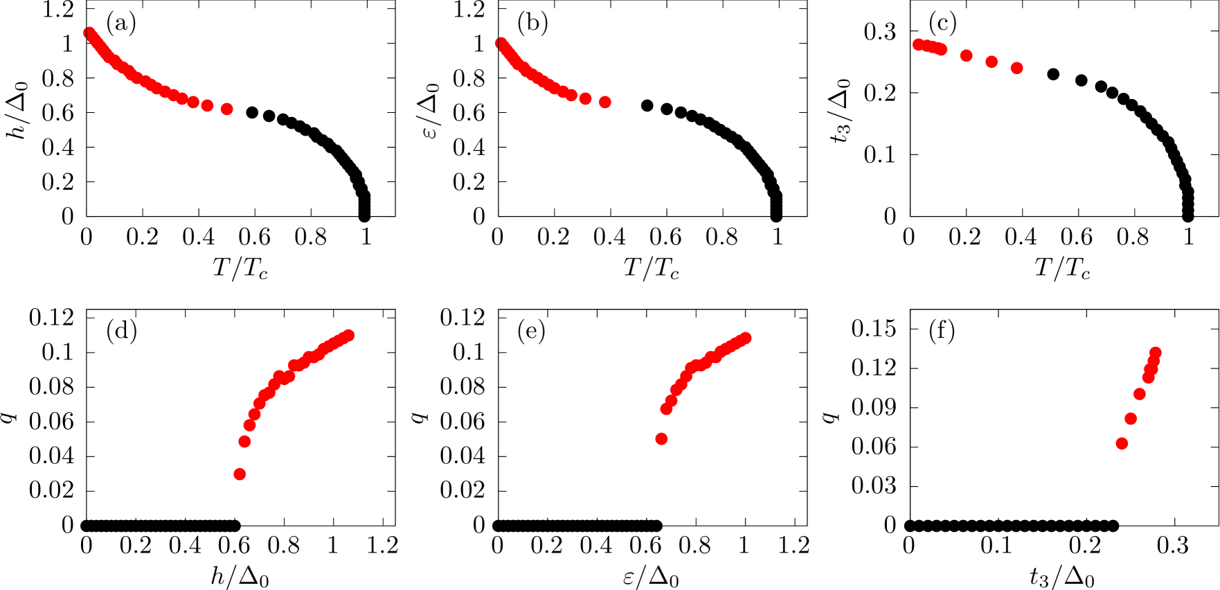
Figure 1: The phase boundary between a normal state and a superconducing state is plotted in (a)-(c), which gives the zeros of the denominator of the pair fluctuation propagator. (a), (b), and (c) represent the results of the conventional SC under Zeeman fields on a square lattice on $h-T$ plane, those of the two-band SC with interband spin-singlet pairing order $(s=-1)$ on a square lattice on $\varepsilon-T$ plane, those of the $j=3/2$ SC on a cubic lattice on $t_{3}-T$ plane, respectively. The transition point to a uniform (nonuniform) state is plotted by the black (red) dot. The magnitude of the center of mass momentum of the Cooper pair $q$ at the transition point is plotted as a function of $h$ for the conventional SC in (d), as a function of $\varepsilon$ for the two-band SC $(s=-1)$ in (e), and as a function of $t_{3}$ for the $j=3/2$ SC in (f), respectively. The dots are colored in the same way as (a)-(c).

To demonstrate the effects of odd-frequency pairs in the transition to a nonuniform superconducting state, we revisit the transition to the FFLO phase in a conventional SC [1, 2]. We consider a spin-singlet superconductivity under Zeeman fields on a square lattice. In Eq. (1), we choose

$$\hat{\xi}_{\bm{k}} =\xi_{\bm{k}}\hat{\sigma}_{0}-\bm{h}\cdot\hat{\bm{\sigma}},\quad\hat{w}(\bm{k})=\frac{1}{\sqrt{2}}(i\hat{\sigma}_{2}),$$ (15)

$$\xi_{\bm{k}} =-2t(\cos k_{x}+\cos k_{y})+4t-\mu,$$ (16)

where $\bm{h}\coloneqq\mu_{\mathrm{B}}\bm{B}$ represents the Zeeman term, $\hat{\sigma}_{\mathrm{i}}$ for $\mathrm{i}=1-3$ are Pauli matrices in the spin space and $\hat{\sigma}_{0}$ is the unit matrix. The pair potential in the BdG Hamiltonian for a uniform phase reads, $\hat{\Delta}(\bm{k})=\Delta(i\hat{\sigma}_{2})$. To proceed with analytic calculations, we consider the continuous limit in this model: $\xi_{\bm{k}}\rightarrow(k_{x}^{2}+k_{y}^{2})/2m-\mu$ with $m=1/2t$ and $\frac{1}{N}\sum_{\bm{k}}\rightarrow\frac{1}{V_{\mathrm{vol}}}\sum_{\bm{k}}$ with $V_{\mathrm{vol}}$ being the volume of the system. By solving the Gor’kov equation in Eq. (95), the anomalous Green’s function is calculated as [8]

$$\hskip 10.00002pt\hat{\mathcal{F}}_{\mathrm{z}}(\bm{k},i\omega_{\ell})=$$

$$\hskip 20.00003pt\frac{-1}{Z_{\mathrm{z}}}\left[\omega_{\ell}^{2}+\xi_{\bm{k}}^{2}+\Delta^{2}-h^{2}+2i\omega_{\ell}\,\bm{h}\cdot\hat{\bm{\sigma}}\right]\Delta(i\hat{\sigma}_{2}),$$ (17)

$$\hskip 10.00002ptZ_{\mathrm{z}}=\xi_{\bm{k}}^{4}+2\,\xi_{\bm{k}}^{2}\,A_{\mathrm{z}}+C_{\mathrm{z}},$$ (18)

$$\hskip 10.00002ptA_{\mathrm{z}}=\omega_{\ell}^{2}-h^{2}+\Delta^{2},\quad C_{\mathrm{z}}=A^{2}_{\mathrm{z}}+4\omega_{\ell}^{2}\,h^{2},$$ (19)

where the last term in Eq. (17) represents the odd-frequency pairing correlation induced by the Zeeman field [32, 33]. The expression of the normal Green’s function $\hat{\mathcal{G}}_{\mathrm{z}}$ is presented in Appendix B. By using the obtained Green’s function, the GL coefficient $a_{\mathrm{z}}(T)$ and the Meissner kernel $K_{{\mathrm{z}},\mu\nu}$ are calculated as

$$a_{\mathrm{z}}(T)=\frac{1}{g}-N_{0}\pi T\sum_{\omega_{\ell}}\frac{\omega_{\ell}^{2}}{|\omega_{\ell}|(\omega_{\ell}^{2}+h^{2})},$$ (20)

$$K_{{\mathrm{z}},\mu\nu}(\bm{0},0)=\delta_{\mu\nu}\frac{2ne^{2}}{m}Q_{\mathrm{z}},$$ (21)

$$Q_{\mathrm{z}}=\sqrt{2}\pi T\sum_{\omega_{\ell}}\frac{\Delta^{2}\left\{A_{\mathrm{z}}^{3}+\sqrt{C_{\mathrm{z}}}(A_{\mathrm{z}}^{2}-2\omega_{\ell}^{2}h^{2})\right\}}{[C_{\mathrm{z}}(A_{\mathrm{z}}+\sqrt{C_{\mathrm{z}}})]^{3/2}}.$$ (22)

where $n=k_{F}^{2}/4\pi$ and $N_{0}=n/\mu$ are the electron density per spin and the density of states per spin, respectively. To obtain Eqs. (20) and (21), the momentum summation is replaced by the integration with respect to $\xi$: $\frac{1}{V_{\mathrm{vol}}}\sum_{\bm{k}}\rightarrow N_{0}\int d\xi$. To derive Eq. (21), we subtracted and added the diamagnetic contribution in the normal state to avoid the formal divergence of the integrand [34].

Eq. (14) becomes

$$a(T_{\bm{q}})+\left.\frac{n\,Q(T_{\bm{q}})}{4m|\Delta|^{2}}\right|_{\Delta=0}q^{2}=0,$$ (23)

with $a=a_{\mathrm{z}}$ and $Q=Q_{\mathrm{z}}$ in the present case. We solve $[D_{\mathrm{s}}^{\mathrm{R}}(\bm{q},0)]^{-1}=0$ numerically on the tight-binding model, which corresponds to Eq. (23) when we consider $q\ll 1$ and then take the continuous limit. We show the solution on $h-T$ plane in Fig. 1(a). The horizontal axis is normalized to $T_{c}$ which is the transition temperature at $h=0$. The vertical axis is normalized to $\Delta_{0}\coloneqq\pi e^{-C}T_{c}=1.76T_{c}$ which is the amplitude of the pair potential at $h=T=0$ with $C=0.577$ being the Euler’s constant [35]. In the numerical simulation, we choose $\mu=t$ and $T_{c}=0.05t$. To obtain Fig. 1(a), we choose $\bm{q}=(q,0)$. The abscissa of the black dot corresponds to the transition temperature $T_{\bm{0}}$ to a uniform superconducting state with $q=0$. Such a transition occurs in weak Zeeman fields. The abscissa of the red dot corresponds to the transition temperature $T_{\bm{q}}$ to a nonuniform superconducting state with $q\neq 0$. The transition temperature $T_{\bm{q}}$ decreases with increasing Zeeman fields and vanishes at $h\sim\Delta_{0}$. The dependence of $q$ on $h$ in (d) shows the monotonic increases of $q$ with increasing $h$. The phase boundary in Fig. 1(a) slightly deviates from those in the circular Fermi surface [36, 37] because the direction of $\bm{q}=(q,0)$ meets a good nesting condition on the anisotropic Fermi surface [38, 39, 40].

The transition to a nonuniform superconducting state is a result of $Q_{\mathrm{z}}<0$ in Eq. (22), where the last term in the numerator is derived from the odd-frequency pairing correlations. Namely, odd-frequency pairs decrease the Meissner kernel with increasing $h$ and change its sign to negative in strong enough Zeeman fields [8]. The appearance of the FFLO state is usually considered as a result of the destruction of Cooper pairs composed of Kramers partners by TRSB perturbations. This interpretation is reasonable and gives a good physical picture of the phenomenon. However, the equations in Eqs. (22) and (23) suggest us an alternative understanding of the FFLO state. Namely, the suppression of the Meissner kernel by induced odd-frequency Cooper pairs stabilizes the FFLO state. If such an interpretation is correct, nonuniform superconducting states would be possible in time-reversal symmetry preserving SCs. In the next section, we will discuss two examples of such SCs. In these cases, the amplitude of odd-frequency Cooper pairs can become large enough to change the sign of the Meissner kernel.

IV Nonuniform superconducting states preserving time-reversal symmetry

In this section, we discuss two examples of nonuniform superconducting states in time-reversal symmetry preserving SCs. One is a two-band SC with interband pair potentials. The other is a $j=3/2$ SC with pseudospin-quintet pair potentials. Odd-frequency Cooper pairs are induced by band-hybridization and/or band-asymmetry in a two-band SC and by spin-orbit interactions in a $j=3/2$ SC.

IV.1 Two-band superconductors with interband pair potentials

We consider a two-band superconductor on a two-dimensional tight-binding square lattice. In Eq. (1), we choose

$$\hat{\xi}_{\bm{k}}=\xi_{\bm{k}}\hat{\rho}_{0}\hat{\sigma}_{0}+\varepsilon\hat{\rho}_{3}\hat{\sigma}_{0}+V\hat{\rho}_{1}\hat{\sigma}_{0},$$ (24)

$$\xi_{\bm{k}}=-2t(\cos k_{x}+\cos k_{y})+4t-\mu,$$ (25)

$$\hat{w}(\bm{k})=\frac{1}{\sqrt{2}}\left[\begin{array}[]{cccc}&&&1\\ &&s&\\ &-s&&\\ -1&&&\end{array}\right]=\begin{cases}\frac{1}{\sqrt{2}}(i\hat{\rho}_{2})\hat{\sigma}_{1}&(s=+1)\\ \frac{1}{\sqrt{2}}\hat{\rho}_{1}(i\hat{\sigma}_{2})&(s=-1)\end{cases},$$ (30)

where $\hat{\rho}_{\mathrm{i}}$ for $\mathrm{i}=1-3$ are Pauli matrices in band space, and $\hat{\rho}_{0}$ is the unit matrix. The asymmetry and the hybridization between the two bands are represented by $\varepsilon$ and $V$, respectively. The pair potential matrix in $s$-wave symmetry reads,

$$\hat{\Delta}=\begin{cases}\Delta(i\hat{\rho}_{2})\hat{\sigma}_{1}&(s=+1)\\ \Delta\hat{\rho}_{1}(i\hat{\sigma}_{2})&(s=-1)\end{cases},$$ (31)

where $s=+1(-1)$ represents the odd-band-parity spin-triplet (even-band-parity spin-singlet) superconducting order. The $8\times 8$ BdG Hamiltonian can be block-diagonalized and the reduced $4\times 4$ Hamiltonian is represented by

$$\check{H}(\bm{k})=\left[\begin{array}[]{cc}\hat{H}_{\mathrm{N}}&\hat{\Delta}\\ \hat{\Delta}^{{\dagger}}&-\hat{H}_{\mathrm{N}}\end{array}\right],$$ (34)

$$\hat{H}_{\mathrm{N}}=\xi_{\bm{k}}\hat{\rho}_{0}+\varepsilon\hat{\rho}_{3}+V\hat{\rho}_{1}.$$ (35)

For odd-band-parity spin-triplet $(s=+1)$ symmetry class, it has been already reported that the transition to a uniform superconducting phase becomes discontinuous for large enough $V$ or large enough $\varepsilon$ [29, 8].

Let us first discuss the results for $s=+1$. The anomalous Green’s function in the reduced subspace in the uniform superconducing state is calculated as [8]

$$\hat{\mathcal{F}}_{+}(\bm{k},i\omega_{\ell})=\frac{-1}{Z_{+}}\left[\omega_{\ell}^{2}+\xi_{\bm{k}}^{2}-\varepsilon^{2}-V^{2}+\Delta^{2}\right.$$

$$\hskip 100.00015pt\left.-2i\omega_{\ell}(\varepsilon\hat{\rho}_{3}+V\hat{\rho}_{1})\right]\Delta(i\hat{\rho}_{2}),$$ (36)

$$Z_{+}=\xi_{\bm{k}}^{4}+2\,\xi_{\bm{k}}^{2}\,A_{+}+C_{+}=Z_{\mathrm{z}}|_{h\rightarrow\sqrt{\varepsilon^{2}+V^{2}}},$$ (37)

$$A_{+}=\omega_{\ell}^{2}-\varepsilon^{2}-V^{2}+\Delta^{2},$$ (38)

$$C_{+}=A^{2}_{+}+4\omega_{\ell}^{2}\,(\varepsilon^{2}+V^{2}).$$ (39)

Both the band hybridization $V$ and the band asymmetry $\varepsilon$ induce the pairing correlations belonging to the odd-frequency symmetry class. The BdG Hamiltonian is totally equivalent to that of a conventional spin-singlet superconductor under Zeeman fields in Sec. III. The GL coefficient and the Meissner kernel have the same structure as those in Eqs. (20), (21) and (22). In the continuous limit, the results are represented as

$$a_{+}(T)=\frac{1}{g}-2N_{0}\pi T\sum_{\omega_{\ell}}\frac{\omega_{\ell}^{2}}{|\omega_{\ell}|(\omega_{\ell}^{2}+\varepsilon^{2}+V^{2})},$$ (40)

$$K_{+,\mu\nu}(\bm{0},0)=\delta_{\mu\nu}\frac{4ne^{2}}{m}Q_{+},$$ (41)

$$Q_{+}=Q_{\mathrm{z}}|_{h\rightarrow\sqrt{\varepsilon^{2}+V^{2}}},$$ (42)

where $Q_{\mathrm{z}}$ is defined in Eq. (22). Therefore, $K_{+,\mu\nu}$ changes the sign to negative for large enough $\sqrt{\varepsilon^{2}+V^{2}}$ [8]. The results in Fig. 1(a) and (d) with replacing $h$ by $\sqrt{\varepsilon^{2}+V^{2}}$ recover the phase boundary and $q$ in the nonuniform states for $s=+1$ with the same parameters in Sec. III: $\mu=t$, $T_{c}=0.05t$, $\Delta_{0}=\pi e^{-C}T_{c}$, and $\bm{q}=(q,0)$.

For $s=-1$, we obtain

$$\hat{\mathcal{F}}_{-}(\bm{k},i\omega_{\ell})=\frac{-1}{Z_{-}}\left[\omega_{\ell}^{2}+\xi_{\bm{k}}^{2}-\varepsilon^{2}+V^{2}+\Delta^{2}\right.$$

$$\hskip 60.00009pt\left.-2(\xi_{\bm{k}}V\hat{\rho}_{1}-i\varepsilon V\hat{\rho}_{2}+i\omega_{\ell}\varepsilon\hat{\rho}_{3})\right]\Delta\hat{\rho}_{1},$$ (43)

$$Z_{-}=\xi_{\bm{k}}^{4}+2\,\xi_{\bm{k}}^{2}\,A_{-}+C_{-},$$ (44)

$$A_{-}=A_{+},$$ (45)

$$C_{-}=A^{2}_{-}+4\left(\omega_{\ell}^{2}\varepsilon^{2}+\omega_{\ell}^{2}V^{2}+V^{2}\Delta^{2}\right).$$ (46)

The band hybridization $V$ induces the subdominant even-frequency pairing correlation, whereas the band asymmetry $\varepsilon$ induces both even-frequency and odd-frequency pairing correlations. The GL coefficient and the Meissner kernel result in

$$a_{-}(T)=\frac{1}{g}-2N_{0}\pi T\sum_{\omega_{\ell}}\frac{\omega_{\ell}^{2}+V^{2}}{|\omega_{\ell}|(\omega_{\ell}^{2}+\varepsilon^{2}+V^{2})},$$ (47)

$$K_{-,\mu\nu}(\bm{0},0)=\delta_{\mu\nu}\frac{4ne^{2}}{m}Q_{-},$$ (48)

$$Q_{-}=\sqrt{2}\pi T\sum_{\omega_{\ell}}\frac{\Delta^{2}}{[C_{-}(A_{-}+\sqrt{C_{-}})]^{3/2}}$$

$$\times\left[A_{-}^{3}+\sqrt{C_{-}}(A_{-}^{2}-2\omega_{\ell}^{2}\varepsilon^{2})\right.$$

$$\hskip 10.00002pt\left.+2V^{2}\left\{C_{-}+2(\omega_{\ell}^{2}+\Delta^{2})(A_{-}+\sqrt{C_{-}})\right\}\right].$$ (49)

While $\varepsilon$ reduces $K_{-,\mu\nu}$ and changes its sign to negative, $V$ increases the Meisner kernel. The results suggest that a nonuniform superconducting state would appear for large enough $\varepsilon$. To confirm the statement, we numerically solve $[D_{\mathrm{s}}^{\mathrm{R}}(\bm{q},0)]^{-1}=0$ on the tight-binding model. The parameters in the numerical simulation are the same as those in Sec. III and $s=+1$: $\mu=t$, $T_{c}=0.05t$, $\Delta_{0}=\pi e^{-C}T_{c}$, and $\bm{q}=(q,0)$. The results for $V=0.3\Delta_{0}$ are shown on $\varepsilon-T$ plane in Fig. 1(b). The amplitude of $q$ at the transition point is also shown as a function of $\varepsilon$ in (e). The transition to nonuniform superconducting states occurs for $\varepsilon\gtrsim 0.6\Delta_{0}$ as indicated by the red dots in (b). The characteristic properties in (b) and (e) are totally the same as those in (a) and (d). The nonuniform superconducting state appears in a time-reversal preserving two-band SC when the amplitude of odd-frequency Cooper pairs is large enough.

IV.2 $j=3/2$ superconductor with a pseudospin-quintet pair potential

Nonuniform states are also stabilized in a $j=3/2$ SC, where an electron has high-pseudospin due to the strong coupling between orbitals with angular momentum $\ell=1$ and spin with $s=1/2$. Here, we consider $s$-wave pseudospin-quintet pairing order on a simple cubic lattice. To describe the electronic structure, we choose

$$\hat{\xi}_{\bm{k}} =\xi_{\bm{k}}1_{4\times 4}+\vec{\epsilon}_{\bm{k}}\cdot\vec{\gamma},\quad\hat{w}(\bm{k})=\frac{1}{\sqrt{2}}\gamma^{4}U_{T},$$ (50)

$$\xi_{\bm{k}} =\left(-2t_{1}-\frac{5}{2}t_{2}\right)\sum_{\nu}\cos{k_{\nu}}+6t_{1}+\frac{15}{2}t_{2}-\mu,$$ (51)

$$\epsilon_{\bm{k},1} =4\sqrt{3}t_{3}\sin{k_{x}}\sin{k_{y}},$$ (52)

$$\epsilon_{\bm{k},2} =4\sqrt{3}t_{3}\sin{k_{y}}\sin{k_{z}},$$ (53)

$$\epsilon_{\bm{k},3} =4\sqrt{3}t_{3}\sin{k_{z}}\sin{k_{x}},$$ (54)

$$\epsilon_{\bm{k},4} =\sqrt{3}t_{2}(-\cos{k_{x}}+\cos{k_{y}}),$$ (55)

$$\epsilon_{\bm{k},5} =t_{2}(-2\cos{k_{z}}+\cos{k_{x}}+\cos{k_{y}}),$$ (56)

$$U_{T} =\gamma^{1}\gamma^{2},$$ (57)

in Eq. (1) [41, 42, 30, 43, 44, 45]. In this Hamiltonian, $\xi_{\bm{k}}$ represents kinetic energy of an electron and the five-component vector $\vec{\epsilon}_{\bm{k}}=(\epsilon_{\bm{k},1},\epsilon_{\bm{k},2},\epsilon_{\bm{k},3},\epsilon_{\bm{k},4},\epsilon_{\bm{k},5})$ determines the dependence of the normal-state dispersions on pseudospins. The definitions of five $4\times 4$ matrices $\gamma^{\mathrm{j}}$ for $\mathrm{j}=1-5$ and important algebras are given in Appendix C for completeness. The corresponding pair potential matrix reads, $\hat{\Delta}(\bm{k})=\Delta\gamma^{4}U_{T}$. For simplicity, we set to $t_{2}=0$. The anomalous Green’s function for a uniform superconducting state is calculated as [8]

$$\hat{\mathcal{F}}_{3/2}(\bm{k},i\omega_{\ell})=-\frac{\Delta}{Z_{3/2}}\left[W-2i\omega_{\ell}\vec{\epsilon}_{\bm{k}}\cdot\vec{\gamma}\right]\gamma^{4}U_{T},$$ (58)

$$Z_{3/2}=W^{2}+4\omega_{\ell}^{2}\vec{\epsilon}_{\bm{k}}^{\,2},\quad W=\omega_{\ell}^{2}+\xi_{\bm{k}}^{2}-\vec{\epsilon}_{\bm{k}}^{\,2}+\Delta^{2}.$$ (59)

The spin-orbit interaction $\vec{\epsilon}_{\bm{k}}$ induces the subdominant odd-frequency pairing correlation represented by the second term in Eq. (58). The GL coefficient and the contribution of the anomalous Green’s function to the Meissner kernel $K^{\mathcal{F}}$ in the lattice model reads [8],

$$a_{3/2}(T)=\frac{1}{g}-2T\sum_{\omega_{\ell}}\frac{1}{N}\sum_{\bm{k}}\frac{1}{Z_{3/2}|_{\Delta=0}}(\omega_{\ell}^{2}+\xi_{\bm{k}}^{2}-\vec{\epsilon}_{\bm{k}}^{\,2}),$$ (60)

$$K^{\mathcal{F}}_{3/2,xx}(\bm{0},0)=$$

$$\hskip 10.00002pt16e^{2}T\sum_{\omega_{\ell}}\frac{1}{N}\sum_{\bm{k}}t^{2}_{1}\sin^{2}k_{x}\frac{\Delta^{2}}{Z_{3/2}^{2}}\left[W^{2}-4\omega_{\ell}^{2}\,\vec{\epsilon}_{\bm{k}}^{\,2}\right],$$ (61)

where we neglect the correction to the velocity operator from the weak spin-orbit interaction $(t_{3}\ll t_{1})$ for simplicity [8]. The second term in Eq. (61) represents the contribution of the subdominant odd-frequency pair and this term reduces the Meissner kernel. Therefore, in $j=3/2$ superconductors, the nonuniform superconducting state can be stabilized by odd-frequency pairs when the spin-orbit interaction is large enough.

To confirm the existence of the stable nonuniform superconducting phase, we plot the solutions of $[D_{\mathrm{s}}^{\mathrm{R}}(\bm{q},0)]^{-1}=0$ on $t_{3}-T$ plane and the amplitude of $q$ in Fig. 1(c) and (f), respectively. In the numerical simulation, we choose $\mu=t_{1}$, $t_{2}=0$, $T_{c}=0.05t_{1}$, $\Delta_{0}=\pi e^{-C}T_{c}$, and $\bm{q}=(q,0,0)$. The characteristic properties found in (c) and (f) are qualitatively the same as those in (a) and (d). The results suggest that odd-frequency Cooper pairs are responsible for the nonuniform phase. It is widely accepted that Eq. (50) describes general electronic structures which have four internal degrees of freedom and preserve both time-reversal symmetry and inversion symmetry [46]. Therefore, the possibility of nonuniform states is a common property among various multiband/orbital SCs.

V Discussion

V.1 Role of symmetry breaking perturbations

TRSB fields have been considered to be essential ingredients for realizing the FFLO (nonuniform) states. In fact, a lot of theoretical and experimental studies have been devoted to the search for superconductivity that survives in strong magnetic fields near the Pauli limit [47, 48, 36]. Here we will examine another physical point of view on an importance of TRSB fields. As we have discussed in the previous sections, odd-frequency Cooper pairs play a key role in the following argument. When an attractive interaction works between the Kramers partners, the pair potential matrix in the BdG Hamiltonian can be expressed by $\hat{\Delta}(\bm{k})=\Delta(\bm{k})\hat{U}_{T}$ with $\Delta(\bm{k})$ being an even function of $\bm{k}$. The matrix $\hat{U}_{T}$ is the unitary part of the time-reversal operator $\mathcal{T}=\hat{U}_{T}\,\mathcal{C}$, where $\mathcal{C}$ means taking the complex conjugation and applying the transformation $\bm{k}\to-\bm{k}$. Generally speaking, the BdG Hamiltonian for uniform superconducting states has a form

$$H_{\mathrm{BdG}}(\bm{k})=\left[\begin{array}[]{cc}\hat{\xi}_{\bm{k}}&\hat{\Delta}(\bm{k})\\ -\hat{\Delta}^{\ast}(-\bm{k})&-\hat{\xi}_{-\bm{k}}^{\ast}\end{array}\right].$$ (64)

The anomalous Green’s function as a solution of the Gor’kov equation is formally expressed by

$$\hat{\mathcal{F}}(\bm{k},i\omega_{\ell}) =\left[\hat{\Delta}(\bm{k})\hat{\Delta}^{\ast}(-\bm{k})-\omega_{\ell}^{2}-\hat{\Delta}(\bm{k})\hat{\xi}^{\ast}_{-\bm{k}}\hat{\Delta}^{-1}(\bm{k})\hat{\xi}_{\bm{k}}\right.$$

$$\hskip 10.00002pt\left.-i\omega_{\ell}\hat{P}_{\mathrm{O}}(\bm{k})\hat{\Delta}^{-1}(\bm{k})\right]^{-1}\hat{\Delta}(\bm{k}),$$ (65)

$$\hat{P}_{\mathrm{O}}(\bm{k}) \coloneqq\hat{\xi}_{\bm{k}}\hat{\Delta}(\bm{k})-\hat{\Delta}(\bm{k})\hat{\xi}^{\ast}_{-\bm{k}},$$ (66)

where $\hat{P}_{\mathrm{O}}(\bm{k})$ represents the existence of odd-frequency Cooper pairs [20, 49, 50]. In this case, the equation

$$\hat{P}_{\mathrm{O}}(\bm{k}) =\left[\hat{\xi}_{\bm{k}}-\hat{U}_{T}\hat{\xi}^{\ast}_{-\bm{k}}\hat{U}_{T}^{-1}\right]\hat{\Delta}(\bm{k}),$$

$$=\left[\hat{\xi}_{\bm{k}}-\mathcal{T}\,\hat{\xi}_{\bm{k}}\,\mathcal{T}^{-1}\right]\hat{\Delta}(\bm{k}),$$ (67)

holds true. Therefore, the condition for the appearance of odd-frequency pairs in this case is identical to that for the presence of TRSB perturbations in the normal state Hamiltonian. However, the condition for the appearance of odd-frequency pairs is broader than that for the presence of TRSB perturbations. Indeed, as we discussed in Sec. IV.1, a band asymmetry induces odd-frequency pairs and stabilizes the nonuniform states in a two-band SC with an $s$-wave spin-singlet pair potential.

TRSB fields have been considered as a necessary item for a nonuniform superconducting state. Here we discuss the validity of the statement. We first discuss superconducting states in spin $s=1/2$ electron system. The normal state Hamiltonian includes two types of spin active potentials:

$$\hat{\xi}_{\bm{k}} =\xi_{\bm{k}}+\bm{h}_{\bm{k}}\cdot\hat{\bm{\sigma}}+\bm{\lambda}_{\bm{k}}\cdot\hat{\bm{\sigma}},$$ (68)

where $\bm{h}_{\bm{k}}=\bm{h}_{-\bm{k}}$ is a TRSB field such as a Zeeman field, ferromagnetic exchange field [47, 48, 51, 52, 32] and an altermagnetic exchange field [53, 54, 55, 56, 57, 58, 59, 60], and $\bm{\lambda}_{\bm{k}}=-\bm{\lambda}_{-\bm{k}}$ represents antisymmetric spin-orbit interactions [61, 62, 63]. The pair potential is represented by

$$\hat{\Delta}(\bm{k}) =(\Delta_{\bm{k}}+\bm{d}_{\bm{k}}\cdot\hat{\bm{\sigma}})i\hat{\sigma}_{2},$$ (69)

where $\Delta_{\bm{k}}=\Delta_{-\bm{k}}$ and $\bm{d}_{\bm{k}}=-\bm{d}_{-\bm{k}}$ represent an even-parity spin-singlet pair potential and an odd-parity spin-triplet pair potential, respectively. The results of induced odd-frequency pairs due to the spin active potentials are listed in Table. 1. For a spin-singlet superconductor, odd-frequency Cooper pairs belonging to spin-triplet even-parity class are generated by the magnetic moment breaking time-reversal symmetry. For a spin-triplet superconductor, two types of odd-frequency Cooper pairs are generated: spin-singlet odd-parity and spin-triplet even-parity. The former is generated by the magnetic moment. But the latter is induced by the spin-orbit interaction preserving time-reversal symmetry. Therefore, TRSB fields are not always necessary to decrease the superfluid density. It is noted that $\bm{\lambda}_{\bm{k}}\times\bm{d}_{\bm{k}}=0$ pointed out in Ref. [62, 63] satisfies the condition to realize a stable superconducting state. Namely, $T_{c}$ for $\bm{\lambda}_{\bm{k}}\times\bm{d}_{\bm{k}}=0$ is higher than that for $\bm{\lambda}_{\bm{k}}\times\bm{d}_{\bm{k}}\neq 0$ [26]. In this sense, it is difficult to stabilize nonuniform superconductivity with time-reversal symmetry when we only consider the case $\bm{\lambda}_{\bm{k}}\times\bm{d}_{\bm{k}}=0$.

The above situation changes when internal degrees of freedom of an electron are enlarged. Examples in Sec. IV suggest that spin, band/orbital, and sublattice are important for nonuniform superconductivity. Our results show that the potentials that hybridize the Hilbert space for each degree of freedom and/or break the symmetry are necessary for appearing a nonuniform superconductivity. To make this point clear, let us consider a two-band superconductor as we did in Sec. IV.1, where Pauli matrices $\hat{\rho}_{\mathrm{i}}$ describe a $2\times 2$ band space in the normal state Hamiltonian. The interband pair potential can be described as $\Delta\,\hat{\rho}_{1}$ and we begin the argument with an even-band-parity pair potential. The normal state Hamiltonian $\hat{\xi}_{\bm{k}}$ includes three types of potentials acting on the band degree of freedom:

$$\hat{\xi}_{\bm{k}} =\xi_{\bm{k}}+V\hat{\rho}_{1}+V^{\prime}\hat{\rho}_{2}+\varepsilon\hat{\rho}_{3},$$ (70)

where $V$ and $V^{\prime}$ represent the band hybridization, and $\varepsilon$ represents the band asymmetry. Eq. (66) becomes $\hat{P}_{\mathrm{O}}=2i\Delta\varepsilon\hat{\rho}_{2}$, which indicates the appearance of odd-frequency odd-band-parity Cooper pairs. In Table. 2, we summarize the matrix structures of the pair potential and those of induced odd-frequency Cooper pairs. For all even-band parity pair potentials, the band hybridization or band asymmetry generates odd-frequency Cooper pairs belonging to odd-band-parity symmetry. When we begin the argument with odd-band-parity pair potential $\Delta\hat{\rho}_{2}$, induced odd-frequency pairs belong to even-band-parity class. Therefore, potentials that hybridize and/or asymmetrize the internal degree of an electron are important for nonuniform superconductivity.

Finally, we point out a trivial potential that generates odd-frequency Cooper pair. In the presence of vector potential, the normal state Hamiltonian is given by

$$\hat{\xi}_{\bm{k}} =\xi_{\bm{k}}+\frac{e^{2}\bm{A}^{2}}{2m}-\frac{e\hbar}{m}\bm{A}\cdot\bm{k}.$$ (71)

As a vector potential acts on charge of an electron, $\hat{\xi}_{\bm{k}}$ is always proportional to identity matrix in any internal space. We find odd-frequency Cooper pairs described by $\hat{P}_{\mathrm{O}}\propto e\bm{A}\cdot\bm{k}$ belonging to the opposite parity to the pair potential. Indeed, a possibility of FFLO states caused by the vector potentials was discussed in Ref. [64].

Table 1: The pair potential and induced odd-frequency Cooper pairs are summarized for the single band $s=1/2$ superconductors. The normal state Hamiltonian is given in Eq. (68).

Pair potential	$\hat{P}_{\mathrm{O}}$
$\Delta_{\bm{k}}\,i\hat{\sigma}_{2}$	$2\Delta_{\bm{k}}\bm{h}_{\bm{k}}\cdot\hat{\bm{\sigma}}i\hat{\sigma}_{2}$
$\bm{d}_{\bm{k}}\cdot\hat{\bm{\sigma}}\,i\hat{\sigma}_{2}$	$2[\bm{d}_{\bm{k}}\cdot\bm{h}_{\bm{k}}+i(\bm{\lambda}_{\bm{k}}\times\bm{d}_{\bm{k}})\cdot\hat{\bm{\sigma}}]i\hat{\sigma}_{2}$

Table 2: The pair potential and induced odd-frequency Cooper pairs are summarized for the two-band superconductors. The normal state Hamiltonian is given in Eq. (70).

Pair potential	$\hat{P}_{\mathrm{O}}$
$\Delta\,\hat{\rho}_{0}$	$2\Delta V^{\prime}\hat{\rho}_{2}$
$\Delta\,\hat{\rho}_{1}$	$2i\Delta\varepsilon\hat{\rho}_{2}$
$\Delta\,\hat{\rho}_{2}$	$2\Delta(V^{\prime}\hat{\rho}_{0}-i\varepsilon\hat{\rho}_{1}+iV\hat{\rho}_{3})$
$\Delta\,\hat{\rho}_{3}$	$-2i\Delta V\hat{\rho}_{2}$

V.2 Relation to discontinuous transition to a uniform state

In a conventional SC under a Zeeman field, the relation between two transition temperatures

$$T^{{\dagger}}=T_{\mathrm{FFLO}},$$ (72)

holds [36]. $T^{{\dagger}}$ is the temperature at which the transition to a uniform superconducting state changes from continuous to discontinuous [51, 52]. $T_{\mathrm{FFLO}}$ is the transition temperature to a nonuniform state. The reason of the coincidence is explained well by the relation between the Meissner kernel and the quartic coefficient in the GL free-energy for a uniform SC in Eq. (12). In the previous study [8], we found that the superfluid density $Q$ and $b$ are related each other by

$$b\approx A\,\left.Q/|\Delta|^{2}\right|_{\Delta\to 0},$$ (73)

in several superconducting states, where $A>0$ is a constant . The pair fluctuation propagator can be expressed by

$$\left[D^{\mathrm{R}}_{\mathrm{s}}(\bm{q},0)\right]^{-1} \propto a(T)+\tilde{A}\,b(T)\,q^{2}+O(q^{4}),$$ (74)

with $\tilde{A}>0$ being a constant. In such cases, the sign change of superfluid density characterizes $T^{{\dagger}}$ and $T_{\mathrm{FFLO}}$ simultaneously, which explains the coincidence. Eq. (72) holds true as long as the relation in Eq. (73) is satisfied and the quartic terms with respect to $q$ in Eq. (74) are negligible .

The relation between the sign of the superfluid density and the stability of the nonuniform superconducting states was pointed out in a previous paper [67]. In addition, we make clear a close relationship also to the discontinuous transition to a uniform superconducting state. We provide a theoretical framework that explains the reasons for appearing the nonuniform superconducting states in terms of the concept of odd-frequency Cooper pairing. Actually, our theory explains the appearance of the nonuniform states in SCs preserving time-reversal symmetry.

VI Conclusion

We have theoretically discussed a mechanism of nonuniform superconductivity including Fulde-Ferrell-Larkin-Ovchinnikov (FFLO) state in a conventional superconductor. The transition temperature to a superconducting state is characterized by the poles of the pair fluctuation propagator. The analytic expression of the propagator tells us a condition for appearing a nonuniform superconductivity. The transition to a uniform superconducting state occurs when the superfluid density in a uniform superconducting state $Q(T)$ is positive at the transition temperature $T_{\bm{0}}$, (i.e., $Q(T_{\bm{0}})>0$). On the other hand for $Q(T_{\bm{0}})<0$, the transition temperature to a nonuniform superconducting state $T_{\bm{q}}$ can be larger than $T_{\bm{0}}$. Namely, a superconducting state becomes spatially nonuniform. This conclusion is valid for most superconductors in the weak coupling limit. We derive the analytic expression of the pair fluctuation propagator for three practical superconductors such as a conventional superconductor under a Zeeman field, a two-band superconductor with interband pair potentials, and a $j=3/2$ superconductor. In all cases, the transition to a nonuniform superconducting state occurs for negative superfluid density. The analytic expression of $Q(T)$ indicates that odd-frequency Cooper pairs decrease the superfluid density. Zeeman fields, band-hybridizations (and/or band-asymmetry), and spin-orbit interactions generate odd-frequency Cooper pair in a conventional superconductor, two-band superconductor, and $j=3/2$ superconductor, respectively. We conclude that odd-frequency Cooper pairing is a useful concept to understand a mechanism of the transition to a nonuniform superconducting state and that of the discontinuous transition to a uniform superconductiviting state. The two phenomena are closely related to each other because the suppression of the superfluid density by odd-frequency Cooper pair is essential in the phenomena. Our theory provides a fundamental viewpoint to stabilize nonuniform superconductivity and would indicate a way to obtain such superconductivity which is overlooked.

Appendix A Meissner kernel up to $\Delta^{2}$

To discuss the linear response of a uniform superconductor described by $\mathcal{H}$ in Eq. (1) to an external magnetic field, we write the noninteracting Hamiltonian in Eq. (2) in real space:

$$\mathcal{H}_{0} =\sum_{\bm{r}\bm{R}\alpha\beta}\left(-t_{\bm{R}}^{\alpha\beta}-\mu\delta_{\bm{R},\bm{0}}\delta_{\alpha\beta}\right)c^{\dagger}_{\bm{r}+\bm{R}\alpha}c_{\bm{r}\beta}.$$ (75)

The matrix element of the noninteracting Hamiltonian in the momentum space is expressed by the hopping: $\epsilon_{\bm{k}\alpha\beta}=\sum_{\bm{R}}-t^{\alpha\beta}_{\bm{R}}e^{-i\bm{k}\cdot\bm{R}}$. The coupling between an electron and an electromagnetic field is considered through the Peierls phase to the hopping $t^{\alpha\beta}_{\bm{R}}$ in $\mathcal{H}_{0}$ [68, 69]:

$$-t^{\alpha\beta}_{\bm{R}} \rightarrow-t^{\alpha\beta}_{\bm{R}}e^{i\varphi_{\bm{R}}(\bm{r})},$$ (76)

$$\varphi_{\bm{R}}(\bm{r}) =e\int_{\bm{r}}^{\bm{r}+\bm{R}}d\bm{r}\cdot\bm{A}(\bm{r})\approx e\bm{A}(\bm{r}+\bm{R}/2)\cdot\bm{R},$$ (77)

where the approximation in Eq. (77) is justified when the spatial variation of the vector potential is much more slowly than the lattice spacing. We also assume that the Peierls phase is independent of the indices of the internal degrees of freedom of the electron and the vector potential does not affect the effective electron-electron interaction Hamiltonian $\mathcal{H}_{1}$. The current density operator is defined from the variation of the Hamiltonian with respect to the vector potential:

$$\delta\mathcal{H}_{\bm{A}} =\mathcal{H}_{\bm{A}+\delta\bm{A}}-\mathcal{H}_{\bm{A}}=-\sum_{\bm{\ell}}\bm{j}_{\bm{\ell}}\cdot\delta\bm{A}_{\bm{\ell}}+O(\delta A^{2}),$$ (78)

where $\mathcal{H}_{\bm{A}}$ is the total Hamiltonian including the Peierls phase. The current density operator is expressed as

$$\bm{j}_{\bm{\ell}}(t)\coloneqq\sum_{\begin{subarray}{c}\bm{r}\bm{R}\\ \alpha\beta\end{subarray}}ie\bm{R}\ t^{\alpha\beta}_{\bm{R}}\ e^{ie\bm{A}_{\bm{\ell}}\cdot\bm{R}}\ c^{{\dagger}}_{\bm{r}+\bm{R}\alpha}c_{\bm{r}\beta}\ \delta_{\bm{\ell},\bm{r}+\bm{R}/2}.$$ (79)

Within the first order of the vector potential, the current density operator can be decomposed into the paramagnetic and diamagnetic terms,

$$j_{\mu\bm{\ell}}(t) =j^{\mathrm{para}}_{\mu\bm{\ell}}+j^{\mathrm{dia}}_{\mu\bm{\ell}}(t)+O(A^{2}),$$ (80)

$$j^{\mathrm{para}}_{\mu\bm{\ell}} \coloneqq ie\sum_{\begin{subarray}{c}\bm{r}\bm{R}\\ \alpha\beta\end{subarray}}R_{\mu}\ t^{\alpha\beta}_{\bm{R}}\ c^{{\dagger}}_{\bm{r}+\bm{R}\alpha}c_{\bm{r}\beta}\ \delta_{\bm{\ell},\bm{r}+\bm{R}/2},$$ (81)

$$j^{\mathrm{dia}}_{\mu\bm{\ell}}(t) \coloneqq-e^{2}\sum_{\begin{subarray}{c}\bm{r}\bm{R}\\ \alpha\beta\end{subarray}}R_{\mu}R_{\nu}\ t^{\alpha\beta}_{\bm{R}}\ c^{{\dagger}}_{\bm{r}+\bm{R}\alpha}c_{\bm{r}\beta}\ A_{\nu\bm{\ell}}(t)\ \delta_{\bm{\ell},\bm{r}+\bm{R}/2}.$$ (82)

The total Hamiltonian in the presence of a vector potential reads,

$$\mathcal{H}_{\bm{A}}=\mathcal{H}-\sum_{\bm{\ell}}\bm{j}^{\mathrm{para}}_{\bm{\ell}}\cdot\bm{A}_{\bm{\ell}}(t)+O(A^{2}).$$ (83)

We only consider the transverse gauge fields (i.e., $\bm{q}\cdot\bm{A}_{\bm{q}}=0$). The expectation value of the current density is calculated from the linear response theory [70, 71, 72]:

$$\langle j_{\mu\bm{q}}\rangle(\omega) =-K_{\mu\nu}(\bm{q},\omega)A_{\nu\bm{q}}(\omega)$$

$$=\langle j_{\mu\bm{q}}(\omega)\rangle+\Lambda^{\mathrm{R}}_{\mu\nu}(\bm{q},\omega)A_{\nu\bm{q}}(\omega),$$ (84)

where $\langle j_{\mu\bm{q}}(\omega)\rangle$ and $\Lambda^{\mathrm{R}}_{\mu\nu}(\bm{q},\omega)$ are the Fourier component of the average of the current density operator and the current-current correlation function, respectively. Within the mean-field approximation, each is calculated as

$$\langle j_{\mu\bm{q}}(\omega)\rangle =-e^{2}T\sum_{\omega_{\ell}}\frac{1}{N}\sum_{\bm{k}}\mathrm{Tr}\left[\partial_{k_{\mu}}\partial_{k_{\nu}}\hat{\epsilon}_{\bm{k}}\hat{\mathcal{G}}(\bm{k},i\omega_{\ell})\right]e^{i\omega_{\ell}\eta}A_{\nu\bm{q}}(\omega),$$ (85)

$$\Lambda^{\mathrm{R}}_{\mu\nu}(\bm{q},\omega) =\Lambda_{\mu\nu}(\bm{q},i\nu_{n}\rightarrow\omega+i\delta),$$ (86)

$$\Lambda_{\mu\nu}(\bm{q},i\nu_{n}) =\int_{0}^{\beta}d\tau\ \frac{1}{N}\langle T_{\tau}j^{\mathrm{para}}_{\mu\bm{q}}(\tau)j^{\mathrm{para}}_{\nu-\bm{q}}\rangle\ e^{i\nu_{n}\tau}$$ (87)

$$=-e^{2}T\sum_{\omega_{\ell}}\frac{1}{N}\sum_{\bm{k}}\mathrm{Tr}\left[\hat{v}_{\mu}(\bm{k}+\bm{q}/2)\hat{\mathcal{G}}(\bm{k}+\bm{q},i\omega_{\ell}+i\nu_{n})\hat{v}_{\nu}(\bm{k}+\bm{q}/2)\hat{\mathcal{G}}(\bm{k},i\omega_{\ell})\right.$$

$$\hskip 90.00014pt\left.+\hat{v}_{\mu}(\bm{k}+\bm{q}/2)\hat{\mathcal{F}}(\bm{k}+\bm{q},i\omega_{\ell}+i\nu_{n})\hat{\underline{v}}_{\nu}(\bm{k}+\bm{q}/2)\hat{\mathcal{\underline{F}}}(\bm{k},i\omega_{\ell})\right],$$ (88)

where we assumed $\langle j^{\mathrm{para}}_{\mu\bm{q}}\rangle=0$, $\eta$ and $\delta$ are small positive real values, and $\mathcal{G}\,(\mathcal{F})$ is normal (anomalous) Green’s function. The mean-field Hamiltonian and the Green’s function reads,

$$\mathcal{H}^{\mathrm{MF}}=\mathcal{H}_{0}+\mathcal{H}^{\mathrm{MF}}_{1}=\frac{1}{2}\sum_{\bm{k}}\vec{\Psi}^{{\dagger}}_{\bm{k}}H(\bm{k})\vec{\Psi}_{\bm{k}}+\mathrm{const.},$$ (89)

$$H(\bm{k})=\left[\begin{array}[]{cc}\hat{\xi}_{\bm{k}}&\hat{\Delta}(\bm{k})\\ -\hat{\Delta}^{\ast}(-\bm{k})&-\hat{\xi}^{\ast}_{-\bm{k}}\end{array}\right],\quad\vec{\Psi}_{\bm{k}}=\left[\vec{\psi}^{\,\mathrm{T}}_{\bm{k}},\vec{\psi}^{\,\mathrm{{\dagger}}}_{-\bm{k}}\right]^{\,\mathrm{T}},\quad\vec{\psi}_{\bm{k}}=\left[c_{\bm{k}1},c_{\bm{k}2},\cdots,c_{\bm{k}M}\right]^{\mathrm{T}},$$ (92)

$$\left[\begin{array}[]{cc}\hat{\mathcal{G}}&\hat{\mathcal{F}}\\ \hat{\underline{\mathcal{F}}}&\hat{\underline{\mathcal{G}}}\end{array}\right]_{(\bm{k},i\omega_{\ell})}=[i\omega_{\ell}-H(\bm{k})]^{-1},$$ (95)

where $M$ is the number of internal degrees of freedom of the electron, $H(\bm{k})$ is a $2M\times 2M$ matrix, and the mean field is defined by

$$\Delta_{\sigma\sigma^{\prime}}(\bm{k}) \coloneqq w_{\sigma\sigma^{\prime}}(\bm{k})\sum_{\gamma\delta}\frac{g}{N}\sum_{\bm{k}^{\prime}}w^{\ast}_{\gamma\delta}(\bm{k}^{\prime})\langle c_{\bm{k}^{\prime}\gamma}c_{-\bm{k}^{\prime}\delta}\rangle.$$ (96)

The response to a static uniform magnetic field is described by $K_{\mu\nu}(\bm{q}\rightarrow\bm{0},\omega=0)$. We obtain

$$K_{\mu\nu}(\bm{0},0) =e^{2}T\sum_{\omega_{\ell}}\frac{1}{N}\sum_{\bm{k}}\mathrm{Tr}\left[\partial_{k_{\mu}}\partial_{k_{\nu}}\hat{\epsilon}_{\bm{k}}\ \hat{\mathcal{G}}(\bm{k},i\omega_{\ell})e^{i\omega_{\ell}\eta}\right.$$

$$\hskip 80.00012pt\left.+\hat{v}_{\mu}(\bm{k})\hat{\mathcal{G}}(\bm{k},i\omega_{\ell})\hat{v}_{\nu}(\bm{k})\hat{\mathcal{G}}(\bm{k},i\omega_{\ell})+\hat{v}_{\mu}(\bm{k})\hat{\mathcal{F}}(\bm{k},i\omega_{\ell})\hat{\underline{v}}_{\nu}(\bm{k})\hat{\mathcal{\underline{F}}}(\bm{k},i\omega_{\ell})\right].$$ (97)

The contribution of the anomalous Green’s function is defined by

$$K^{\mathcal{F}}_{\mu\nu}(\bm{0},0)\coloneqq e^{2}T\sum_{\omega_{\ell}}\frac{1}{N}\sum_{\bm{k}}\mathrm{Tr}\left[\hat{v}_{\mu}(\bm{k})\hat{\mathcal{F}}(\bm{k},i\omega_{\ell})\hat{\underline{v}}_{\nu}(\bm{k})\hat{\mathcal{\underline{F}}}(\bm{k},i\omega_{\ell})\right],$$ (98)

in Eq. (61). Expanding the Green’s function with respect to $\Delta$, we find

$$K_{\mu\nu}(\bm{0},0)=e^{2}T\sum_{\omega_{\ell}}\frac{1}{N}\sum_{\bm{k}}\mathrm{Tr} \left[\partial_{k_{\mu}}\partial_{k_{\nu}}\hat{\epsilon}\ \hat{\mathcal{G}}_{0}\hat{\Delta}\hat{\mathcal{\underline{G}}}_{0}\hat{\underline{\Delta}}\hat{\mathcal{G}}_{0}e^{i\omega_{\ell}\eta}+\hat{v}_{\mu}\hat{\mathcal{G}}_{0}\hat{v}_{\nu}\hat{\mathcal{G}}_{0}\hat{\Delta}\hat{\mathcal{\underline{G}}}_{0}\hat{\underline{\Delta}}\hat{\mathcal{G}}_{0}\right.$$

$$+\left.\hat{v}_{\mu}\hat{\mathcal{G}}_{0}\hat{\Delta}\hat{\mathcal{\underline{G}}}_{0}\hat{\underline{\Delta}}\hat{\mathcal{G}}_{0}\hat{v}_{\nu}\hat{\mathcal{G}}_{0}+\hat{v}_{\mu}\hat{\mathcal{G}}_{0}\hat{\Delta}\hat{\mathcal{\underline{G}}}_{0}\hat{\underline{v}}_{\nu}\hat{\mathcal{\underline{G}}}_{0}\hat{\underline{\Delta}}\hat{\mathcal{G}}_{0}\right]+O(\Delta^{4}),$$ (99)

where we assumed absence of the Meissner effect in the normal state:

$$K^{\mathrm{N}}_{\mu\nu}(\bm{0},0)\coloneqq e^{2}T\sum_{\omega_{\ell}}\frac{1}{N}\sum_{\bm{k}}\mathrm{Tr} \left[\partial_{k_{\mu}}\partial_{k_{\nu}}\hat{\epsilon}\ \hat{\mathcal{G}}_{0}e^{i\omega_{\ell}\eta}+\hat{v}_{\mu}\hat{\mathcal{G}}_{0}\hat{v}_{\nu}\hat{\mathcal{G}}_{0}\right]=0.$$ (100)

Appendix B Normal Green’s function

The normal Green’s function in a uniform superconducting state of the three theoretical models are summarized in this section. The result for a conventional superconductor under Zeeman potentials in Sec. III reads,

$$\hskip 10.00002pt\hat{\mathcal{G}}_{\mathrm{z}}(\bm{k},i\omega_{\ell})=$$

$$\hskip 20.00003pt\frac{-1}{Z_{\mathrm{z}}}\left[(i\omega_{\ell}+\xi_{\bm{k}})(\omega_{\ell}^{2}+\xi_{\bm{k}}^{2}+\Delta^{2})+(i\omega_{\ell}-\xi_{\bm{k}})h^{2}\right.$$

$$\hskip 30.00005pt\left.+\left\{(i\omega_{\ell}+\xi_{\bm{k}})^{2}-h^{2}+\Delta^{2}\right\}\bm{h}\cdot\hat{\bm{\sigma}}\right].$$ (101)

The result for a two-band superconductor in Sec. IV.1 for $s=+1$ is given by

$$\hat{\mathcal{G}}_{+}(\bm{k},i\omega_{\ell})=$$

$$\frac{-1}{Z_{+}}\left[(i\omega_{\ell}+\xi_{\bm{k}})(\omega_{\ell}^{2}+\xi_{\bm{k}}^{2}+\Delta^{2})+(i\omega_{\ell}-\xi_{\bm{k}})(\varepsilon^{2}+V^{2})\right.$$

$$\left.-\left\{(i\omega_{\ell}+\xi_{\bm{k}})^{2}-(\varepsilon^{2}+V^{2})+\Delta^{2}\right\}(\varepsilon\hat{\rho}_{3}+V\hat{\rho}_{1})\right].$$ (102)

For $s=-1$, we obtain

$$\hat{\mathcal{G}}_{-}(\bm{k},i\omega_{\ell})=$$

$$\frac{-1}{Z_{-}}\left[(i\omega_{\ell}+\xi_{\bm{k}})(\omega_{\ell}^{2}+\xi_{\bm{k}}^{2}+\Delta^{2})+(i\omega_{\ell}-\xi_{\bm{k}})(\varepsilon^{2}+V^{2})\right.$$

$$\hskip 20.00003pt-\left\{(i\omega_{\ell}+\xi_{\bm{k}})^{2}-(\varepsilon^{2}+V^{2})+\Delta^{2}\right\}(\varepsilon\hat{\rho}_{3}+V\hat{\rho}_{1})$$

$$\hskip 20.00003pt\left.+2V\Delta^{2}\hat{\rho}_{1}\right].$$ (103)

In a $j=3/2$ superconductor discussed in Sec. IV.2 with $t_{2}=0$, we obtain

$$\hat{\mathcal{G}}_{3/2}(\bm{k},i\omega_{n})=$$

$$\frac{-1}{Z_{3/2}}\left[(i\omega_{n}+\xi_{\bm{k}})(\omega_{n}^{2}+\xi_{\bm{k}}^{2}+\Delta^{2})+(i\omega_{n}-\xi_{\bm{k}})\vec{\epsilon}_{\bm{k}}^{\,2}\right.$$

$$\hskip 20.00003pt\left.-\left\{(i\omega_{n}+\xi_{\bm{k}})^{2}-\vec{\epsilon}_{\bm{k}}^{\,2}+\Delta^{2}\right\}\vec{\epsilon}_{\bm{k}}\cdot\vec{\gamma}\right].$$ (104)

Appendix C Algebras of $\gamma$ matrices

The angular momentum operators of $j=3/2$ electrons are described by,

$$J_{x} =\frac{1}{2}\left[\begin{array}[]{cccc}0&\sqrt{3}&0&0\\ \sqrt{3}&0&2&0\\ 0&2&0&\sqrt{3}\\ 0&0&\sqrt{3}&0\end{array}\right],$$ (109)

$$J_{y} =\frac{1}{2}\left[\begin{array}[]{cccc}0&-i\sqrt{3}&0&0\\ i\sqrt{3}&0&-2i&0\\ 0&2i&0&-i\sqrt{3}\\ 0&0&i\sqrt{3}&0\end{array}\right],$$ (114)

$$J_{z} =\frac{1}{2}\left[\begin{array}[]{cccc}3&0&0&0\\ 0&1&0&0\\ 0&0&-1&0\\ 0&0&0&-3\end{array}\right].$$ (119)

The five Dirac’s $\gamma$-matrices are defined in $4\times 4$ pseudospin space as

$$\gamma^{1}= \frac{1}{\sqrt{3}}(J_{x}J_{y}+J_{y}J_{x}),\;\gamma^{2}=\frac{1}{\sqrt{3}}(J_{y}J_{z}+J_{z}J_{y}),$$ (120)

$$\gamma^{3}= \frac{1}{\sqrt{3}}(J_{z}J_{x}+J_{x}J_{z}),\;\gamma^{4}=\frac{1}{\sqrt{3}}(J_{x}^{2}-J_{y}^{2}),$$ (121)

$$\gamma^{5}= \frac{1}{3}(2J_{z}^{2}-J_{x}^{2}-J_{y}^{2}),$$ (122)

and $1_{4\times 4}$ is the identity matrix. They satisfy the following relations

$$\gamma^{\mathrm{i}}\,\gamma^{\mathrm{j}}+\gamma^{\mathrm{j}}\,\gamma^{\mathrm{i}}=2\times 1_{4\times 4}\delta_{\mathrm{i},\mathrm{j}},$$ (123)

$$\gamma^{1}\,\gamma^{2}\,\gamma^{3}\,\gamma^{4}\,\gamma^{5}=-1_{4\times 4},$$ (124)

$$\{\gamma^{\mathrm{i}}\}^{\ast}=\{\gamma^{\mathrm{i}}\}^{\mathrm{T}}=U_{T}\,\gamma^{\mathrm{i}}\,U_{T}^{-1},\quad U_{T}=\gamma^{1}\,\gamma^{2},$$ (125)

where $U_{T}$ is the unitary part of the time-reversal operation $\mathcal{T}=U_{T}\,\mathcal{K}$ with $\mathcal{K}$ meaning complex conjugation.

References

- Fulde and Ferrell [1964] P. Fulde and R. A. Ferrell, Superconductivity in a Strong Spin-Exchange Field, Phys. Rev. 135, A550 (1964).
- Larkin and Ovchinnikov [1964] A. I. Larkin and Y. N. Ovchinnikov, Nonuniform state of superconductors, Zh. Eksp. Teor. Fiz. 47, 1136 (1964), [Sov. Phys. JETP 20, 762 (1965)].
- Sumita et al. [2023] S. Sumita, M. Naka, and H. Seo, Fulde-Ferrell-Larkin-Ovchinnikov state induced by antiferromagnetic order in -type organic conductors, Phys. Rev. Res. 5, 043171 (2023).
- Zhang et al. [2024] S.-B. Zhang, L.-H. Hu, and T. Neupert, Finite-momentum Cooper pairing in proximitized altermagnets, Nature Communications 15, 1801 (2024).
- Chakraborty and Black-Schaffer [2024] D. Chakraborty and A. M. Black-Schaffer, Zero-field finite-momentum and field-induced superconductivity in altermagnets, Phys. Rev. B 110, L060508 (2024).
- Mineev and Samokhin [2008] V. P. Mineev and K. V. Samokhin, Nonuniform states in noncentrosymmetric superconductors: Derivation of Lifshitz invariants from microscopic theory, Phys. Rev. B 78, 144503 (2008).
- Li and Brydon [2024] G. Li and P. M. R. Brydon, Collective modes in an unconventional superconductor with fermions, Phys. Rev. B 110, 144501 (2024).
- Sato et al. [2024] T. Sato, S. Kobayashi, and Y. Asano, Discontinuous transition to a superconducting phase, Phys. Rev. B 110, 144503 (2024).
- Tanuma et al. [2009] Y. Tanuma, N. Hayashi, Y. Tanaka, and A. A. Golubov, Model for Vortex-Core Tunneling Spectroscopy of Chiral -Wave Superconductors via Odd-Frequency Pairing States, Phys. Rev. Lett. 102, 117003 (2009).
- Kuzmanovski et al. [2020] D. Kuzmanovski, R. S. Souto, and A. V. Balatsky, Odd-frequency superconductivity near a magnetic impurity in a conventional superconductor, Phys. Rev. B 101, 094505 (2020).
- Perrin et al. [2020] V. Perrin, F. L. N. Santos, G. C. Ménard, C. Brun, T. Cren, M. Civelli, and P. Simon, Unveiling Odd-Frequency Pairing around a Magnetic Impurity in a Superconductor, Phys. Rev. Lett. 125, 117003 (2020).
- Suzuki et al. [2022] S.-I. Suzuki, T. Sato, and Y. Asano, Odd-frequency Cooper pair around a magnetic impurity, Phys. Rev. B 106, 104518 (2022).
- Suzuki et al. [2023] S.-I. Suzuki, T. Sato, A. A. Golubov, and Y. Asano, Fulde-Ferrell-Larkin-Ovchinnikov state in a superconducting thin film attached to a ferromagnetic cluster, Phys. Rev. B 108, 064509 (2023).
- Tanaka and Golubov [2007] Y. Tanaka and A. A. Golubov, Theory of the Proximity Effect in Junctions with Unconventional Superconductors, Phys. Rev. Lett. 98, 037003 (2007).
- Asano and Tanaka [2013] Y. Asano and Y. Tanaka, Majorana fermions and odd-frequency Cooper pairs in a normal-metal nanowire proximity-coupled to a topological superconductor, Phys. Rev. B 87, 104513 (2013).
- Berezinskii [1974] V. L. Berezinskii, New model of the anisotropic phase of superfluid , Pis’ma Zh. Eksp. Teor. Fiz. 20, 628 (1974), [JETP Lett. 20, 287 (1974)].
- Bergeret et al. [2005] F. S. Bergeret, A. F. Volkov, and K. B. Efetov, Odd triplet superconductivity and related phenomena in superconductor-ferromagnet structures, Rev. Mod. Phys. 77, 1321 (2005).
- Tanaka et al. [2012] Y. Tanaka, M. Sato, and N. Nagaosa, Symmetry and Topology in Superconductors -Odd-Frequency Pairing and Edge States-, Journal of the Physical Society of Japan 81, 011013 (2012).
- Linder and Balatsky [2019] J. Linder and A. V. Balatsky, Odd-frequency superconductivity, Rev. Mod. Phys. 91, 045005 (2019).
- Triola et al. [2020] C. Triola, J. Cayao, and A. M. Black-Schaffer, The Role of Odd-Frequency Pairing in Multiband Superconductors, Annalen der Physik 532, 1900298 (2020), https://onlinelibrary.wiley.com/doi/pdf/10.1002/andp.201900298 .
- Cayao et al. [2020] J. Cayao, C. Triola, and A. M. Black-Schaffer, Odd-frequency superconducting pairing in one-dimensional systems, The European Physical Journal Special Topics 229, 545 (2020).
- Asano et al. [2014] Y. Asano, Y. V. Fominov, and Y. Tanaka, Consequences of bulk odd-frequency superconducting states for the classification of Cooper pairs, Phys. Rev. B 90, 094512 (2014).
- Asano et al. [2011] Y. Asano, A. A. Golubov, Y. V. Fominov, and Y. Tanaka, Unconventional Surface Impedance of a Normal-Metal Film Covering a Spin-Triplet Superconductor Due to Odd-Frequency Cooper Pairs, Phys. Rev. Lett. 107, 087001 (2011).
- Suzuki and Asano [2014] S.-I. Suzuki and Y. Asano, Paramagnetic instability of small topological superconductors, Phys. Rev. B 89, 184508 (2014).
- Black-Schaffer and Balatsky [2013] A. M. Black-Schaffer and A. V. Balatsky, Odd-frequency superconducting pairing in multiband superconductors, Phys. Rev. B 88, 104514 (2013).
- Asano and Sasaki [2015] Y. Asano and A. Sasaki, Odd-frequency Cooper pairs in two-band superconductors and their magnetic response, Phys. Rev. B 92, 224508 (2015).
- Cooper [1956] L. N. Cooper, Bound Electron Pairs in a Degenerate Fermi Gas, Phys. Rev. 104, 1189 (1956).
- Ambegaokar [1969] V. Ambegaokar, Superconductivity, edited by R. D. Parks, Vol. 1 (Marcel Dekker, 1969) p. 259.
- Gomes da Silva et al. [2014] M. Gomes da Silva, F. Dinóla Neto, I. Padilha, J. Ricardo de Sousa, and M. Continentino, First-order superconducting transition in the inter-band model, Physics Letters A 378, 1396 (2014).
- Brydon et al. [2016] P. M. R. Brydon, L. Wang, M. Weinert, and D. F. Agterberg, Pairing of Fermions in Half-Heusler Superconductors, Phys. Rev. Lett. 116, 177001 (2016).
- Note [1] The odd order terms would play an important role to discuss other exotic phenomena such as superconducting diode effect [73, 74, 75]. The effect of these terms will be discussed elesewhere.
- Bergeret et al. [2001] F. S. Bergeret, A. F. Volkov, and K. B. Efetov, Long-Range Proximity Effects in Superconductor-Ferromagnet Structures, Phys. Rev. Lett. 86, 4096 (2001).
- Chakraborty and Black-Schaffer [2022] D. Chakraborty and A. M. Black-Schaffer, Interplay of finite-energy and finite-momentum superconducting pairing, Phys. Rev. B 106, 024511 (2022).
- Abrikosov et al. [1975] A. A. Abrikosov, L. P. Gor’kov, and I. E. Dzyaloshinski, Methods of Quantum Field Theory in Statistical Physics (Dover Publications, New York, 1975).
- Tinkham [1996] M. Tinkham, Introduction to Superconductivity (McGraw-Hill, New York, 1996).
- Matsuda and Shimahara [2007] Y. Matsuda and H. Shimahara, Fulde-Ferrell-Larkin-Ovchinnikov State in Heavy Fermion Superconductors, Journal of the Physical Society of Japan 76, 051005 (2007), https://doi.org/10.1143/JPSJ.76.051005 .
- Burkhardt and Rainer [1994] H. Burkhardt and D. Rainer, Fulde-Ferrell-Larkin-Ovchinnikov state in layered superconductors, Annalen der Physik 506, 181 (1994).
- Shimahara [1994] H. Shimahara, Fulde-Ferrell state in quasi-two-dimensional superconductors, Phys. Rev. B 50, 12760 (1994).
- Shimahara [1997] H. Shimahara, Fulde-Ferrell-Larkin-Ovchinnikov State in a Quasi-Two-Dimensional Organic Superconductor, Journal of the Physical Society of Japan 66, 541 (1997), https://doi.org/10.1143/JPSJ.66.541 .
- Yokoyama et al. [2008] T. Yokoyama, S. Onari, and Y. Tanaka, Theory of Fulde–Ferrell–Larkin–Ovchinnikov State of Superconductors with and without Inversion Symmetry: Hubbard Model Approach, Journal of the Physical Society of Japan 77, 064711 (2008), https://doi.org/10.1143/JPSJ.77.064711 .
- Luttinger and Kohn [1955] J. M. Luttinger and W. Kohn, Motion of Electrons and Holes in Perturbed Periodic Fields, Phys. Rev. 97, 869 (1955).
- Sigrist and Ueda [1991] M. Sigrist and K. Ueda, Phenomenological theory of unconventional superconductivity, Rev. Mod. Phys. 63, 239 (1991).
- Agterberg et al. [2017] D. F. Agterberg, P. M. R. Brydon, and C. Timm, Bogoliubov Fermi Surfaces in Superconductors with Broken Time-Reversal Symmetry, Phys. Rev. Lett. 118, 127001 (2017).
- Brydon et al. [2018] P. M. R. Brydon, D. F. Agterberg, H. Menke, and C. Timm, Bogoliubov Fermi surfaces: General theory, magnetic order, and topology, Phys. Rev. B 98, 224509 (2018).
- Roy et al. [2019] B. Roy, S. A. A. Ghorashi, M. S. Foster, and A. H. Nevidomskyy, Topological superconductivity of spin- carriers in a three-dimensional doped Luttinger semimetal, Phys. Rev. B 99, 054505 (2019).
- Cavanagh et al. [2023] D. C. Cavanagh, D. F. Agterberg, and P. M. R. Brydon, Pair breaking in superconductors with strong spin-orbit coupling, Phys. Rev. B 107, L060504 (2023).
- Chandrasekhar [1962] B. S. Chandrasekhar, A NOTE ON THE MAXIMUM CRITICAL FIELD OF HIGH‐FIELD SUPERCONDUCTORS, Applied Physics Letters 1, 7 (1962), https://doi.org/10.1063/1.1777362 .
- Clogston [1962] A. M. Clogston, Upper Limit for the Critical Field in Hard Superconductors, Phys. Rev. Lett. 9, 266 (1962).
- Ramires and Sigrist [2016] A. Ramires and M. Sigrist, Identifying detrimental effects for multiorbital superconductivity: Application to , Phys. Rev. B 94, 104501 (2016).
- Ramires et al. [2018] A. Ramires, D. F. Agterberg, and M. Sigrist, Tailoring by symmetry principles: The concept of superconducting fitness, Phys. Rev. B 98, 024501 (2018).
- Sarma [1963] G. Sarma, On the influence of a uniform exchange field acting on the spins of the conduction electrons in a superconductor, Journal of Physics and Chemistry of Solids 24, 1029 (1963).
- Maki and Tsuneto [1964] K. Maki and T. Tsuneto, Pauli Paramagnetism and Superconducting State, Progress of Theoretical Physics 31, 945 (1964), https://academic.oup.com/ptp/article-pdf/31/6/945/5271369/31-6-945.pdf .
- Šmejkal et al. [2020] L. Šmejkal, R. González-Hernández, T. Jungwirth, and J. Sinova, Crystal time-reversal symmetry breaking and spontaneous Hall effect in collinear antiferromagnets, Science Advances 6, eaaz8809 (2020), https://www.science.org/doi/pdf/10.1126/sciadv.aaz8809 .
- Naka et al. [2019] M. Naka, S. Hayami, H. Kusunose, Y. Yanagi, Y. Motome, and H. Seo, Spin current generation in organic antiferromagnets, Nature Communications 10, 4305 (2019).
- Ahn et al. [2019] K.-H. Ahn, A. Hariki, K.-W. Lee, and J. Kuneš, Antiferromagnetism in as -wave Pomeranchuk instability, Phys. Rev. B 99, 184432 (2019).
- Hayami et al. [2020a] S. Hayami, Y. Yanagi, M. Naka, H. Seo, Y. Motome, and H. Kusunose, Multipole Description of Emergent Spin–Orbit Interaction in Organic Antiferromagnet -(BEDT-TTF)2Cu[N(CN)2]Cl, JPS Conf. Proc. 30, 011149 (2020a), https://journals.jps.jp/doi/pdf/10.7566/JPSCP.30.011149 .
- Hayami et al. [2019] S. Hayami, Y. Yanagi, and H. Kusunose, Momentum-Dependent Spin Splitting by Collinear Antiferromagnetic Ordering, Journal of the Physical Society of Japan 88, 123702 (2019), https://doi.org/10.7566/JPSJ.88.123702 .
- Hayami et al. [2020b] S. Hayami, Y. Yanagi, and H. Kusunose, Bottom-up design of spin-split and reshaped electronic band structures in antiferromagnets without spin-orbit coupling: Procedure on the basis of augmented multipoles, Phys. Rev. B 102, 144441 (2020b).
- Šmejkal et al. [2022a] L. Šmejkal, J. Sinova, and T. Jungwirth, Beyond Conventional Ferromagnetism and Antiferromagnetism: A Phase with Nonrelativistic Spin and Crystal Rotation Symmetry, Phys. Rev. X 12, 031042 (2022a).
- Šmejkal et al. [2022b] L. Šmejkal, J. Sinova, and T. Jungwirth, Emerging Research Landscape of Altermagnetism, Phys. Rev. X 12, 040501 (2022b).
- Gor’kov and Rashba [2001] L. P. Gor’kov and E. I. Rashba, Superconducting 2D System with Lifted Spin Degeneracy: Mixed Singlet-Triplet State, Phys. Rev. Lett. 87, 037004 (2001).
- Frigeri et al. [2004a] P. A. Frigeri, D. F. Agterberg, A. Koga, and M. Sigrist, Superconductivity without Inversion Symmetry: MnSi versus , Phys. Rev. Lett. 92, 097001 (2004a).
- Frigeri et al. [2004b] P. A. Frigeri, D. F. Agterberg, and M. Sigrist, Spin susceptibility in superconductors without inversion symmetry, New Journal of Physics 6, 115 (2004b).
- Shimahara et al. [1996] H. Shimahara, S. Matsuo, and K. Nagai, Nonuniform superconductivity due to the orbital magnetic effect in a d-wave superconductor in a magnetic field, Phys. Rev. B 53, 12284 (1996).
- Note [2] If we do not perform the momentum integration analytically, in Eq. (73\@@italiccorr) is replaced by , which represents the contribution from the anomalous Green’s function to the superfluid density.
- Note [3] Of course, this argument is not valid when the electron correlation in the normal state is very strong [37]. However, the relation would hold true in most superconductors when the correlation is weak.
- Taylor et al. [2006] E. Taylor, A. Griffin, N. Fukushima, and Y. Ohashi, Pairing fluctuations and the superfluid density through the BCS-BEC crossover, Phys. Rev. A 74, 063626 (2006).
- Peierls [1933] R. Peierls, Zur Theorie des Diamagnetismus von Leitungselektronen., Z. Physik 80, 763 (1933).
- Luttinger [1951] J. M. Luttinger, The Effect of a Magnetic Field on Electrons in a Periodic Potential, Phys. Rev. 84, 814 (1951).
- Scalapino et al. [1992] D. J. Scalapino, S. R. White, and S. C. Zhang, Superfluid density and the Drude weight of the Hubbard model, Phys. Rev. Lett. 68, 2830 (1992).
- Scalapino et al. [1993] D. J. Scalapino, S. R. White, and S. Zhang, Insulator, metal, or superconductor: The criteria, Phys. Rev. B 47, 7995 (1993).
- Kostyrko et al. [1994] T. Kostyrko, R. Micnas, and K. A. Chao, Gauge-invariant theory of the Meissner effect in the lattice model of a superconductor with local pairing, Phys. Rev. B 49, 6158 (1994).
- Yuan and Fu [2022] N. F. Q. Yuan and L. Fu, Supercurrent diode effect and finite-momentum superconductors, Proceedings of the National Academy of Sciences 119, e2119548119 (2022), https://www.pnas.org/doi/pdf/10.1073/pnas.2119548119 .
- Daido et al. [2022] A. Daido, Y. Ikeda, and Y. Yanase, Intrinsic Superconducting Diode Effect, Phys. Rev. Lett. 128, 037001 (2022).
- He et al. [2022] J. J. He, Y. Tanaka, and N. Nagaosa, A phenomenological theory of superconductor diodes, New Journal of Physics 24, 053014 (2022).