Grasstopes Might not be Positive Geometries (but Might as well be)

1 Introduction, problems and ideas

We begin with recalling the definition of a positive geometry, following [Lam:2022yly]. Let $X$ be a complex $d$-dimensional irreducible algebraic variety defined over $\mathbb{R}$. We equip the real points $X(\mathbb{R})$ with the analytic topology. Let $X_{\geq 0}\subset X(\mathbb{R})$ be a closed semialgebraic subset such that the interior $X_{>0}=\operatorname{Int}(X_{\geq 0})$ is an oriented $d$-manifold, and the closure of $X_{>0}$ recovers $X_{\geq 0}$. Let $\partial X_{\geq 0}$ denote the boundary $X_{\geq 0}\setminus X_{>0}$ and let $\partial X$ denote the Zariski closure of $\partial X_{\geq 0}$. Let $C_{1},C_{2},\ldots,C_{r}$ be the irreducible components of $\partial X$. Let $C_{i,\geq 0}$ denote the closures of the interior of $C_{i}\cap X_{\geq 0}$ in $C_{i}(\mathbb{R})$. The spaces $C_{1,\geq 0},C_{2,\geq 0},\ldots,C_{r,\geq 0}$ are called the boundary components, or facets of $X_{\geq 0}$.

Definition 1.1.

We call $(X,X_{\geq 0})$ a positive geometry if there exists a unique nonzero rational $d$-form $\Omega(X,X_{\geq 0})$, called the canonical form, satisfying the recursive axioms:

1. If $d=0$, then $X=X_{\geq 0}=\mathrm{pt}$ is a point and we define $\Omega(X,X_{\geq 0})=\pm 1$ depending on the orientation.

2. If $d>0$, then we require that $\Omega(X,X_{\geq 0})$ has poles only along the boundary components $C_{i}$, these poles are simple, and for each $i=1,2,\ldots,r$, we have

   $$\operatorname{Res}_{C_{i}}\Omega(X,X_{\geq 0})=\Omega(C_{i},C_{i,\geq 0}).$$

We now recall some more basic definitions. A totally nonnegative Grassmannian $\text{Gr}_{\geq 0}(k,n)$ is the subset of the real Grassmannian $\text{Gr}(k,n)$ consisting of the points whose Plücker coordinates all have the same sign (zeros are allowed). This set is studied extensively in [postnikov] (also see [Williams:2021zph] for a nice introduction). A positroid cell is a subset of $\text{Gr}_{\geq 0}(k,n)$ consisting of all points whose matrix representatives have the same matroid. A Grassmann polytope (Grasstope) is the image in $\text{Gr}(k,l)$ of a positroid cell under a map $\tilde{Z}$ given by $A\mapsto AZ$ for a fixed $n\times l$ matrix $Z$. Here $A$ is any matrix representative of an element of the positroid cell.

Consider a positroid cell $S$ in $\text{Gr}_{\geq 0}(2,8)$ defined by the conditions $1||2,\leavevmode\nobreak\ 3||4,\leavevmode\nobreak\ 5||6,\leavevmode\nobreak\ 7||8$, that is, by the vanishing of Plücker coordinates $q_{12},q_{34},q_{56},q_{78}$. This cell can be parametrized as follows:

$$\begin{pmatrix}1&a&b&bd&e&eg&0&0\\ 0&0&c&cd&f&fg&h&1\end{pmatrix}$$

with $a,b,c,d,e,f,g,h\geq 0$ and $\frac{b}{c}\geq\frac{e}{f}$. Now consider a map $\tilde{Z}:\text{Gr}_{\geq 0}(2,8)\to\text{Gr}(2,6)$ induced by a totally positive matrix

$$Z=\begin{pmatrix}1&0&0&0&0&0\\ 0&1&0&0&0&0\\ 0&0&1&0&0&0\\ 0&0&0&1&0&0\\ 0&0&0&0&0&1\\ -1&1&-1&1&-1&1\\ -6&5&-4&3&-2&1\\ \end{pmatrix}.$$

The map $\tilde{Z}$ sends $A\in\text{Gr}_{\geq 0}(2,8)$ to $AZ\in\text{Gr}(2,6)$ and, due to $Z$ being totally positive, is well-defined. Our hope is to show that the Grasstope $\tilde{Z}(S)$ is not a positive geometry, thus disproving [arkani2017positive, Conjecture 6.3]. The reason behind this hope is that the map $\tilde{Z}$ has degree $2$ on $S$ (see below), while on all other $8$-dimensional positroid cells in $\text{Gr}_{\geq 0}(2,8)$ it has degree one. This leads to interesting phenomena in the boundary of the resulting Grasstope, which might pose an obstacle to it being a positive geometry. One more indication that this Grasstope might not be a positive geometry is the following observation.

An Observation from Thomas Lam. Even if $\tilde{Z}(S)$ is a positive geometry, its canonical form cannot be the pushforward of the canonical form of $S$ under $\tilde{Z}$, since this latter form only has linear and quadratic poles (this still needs to be checked, but this is computable), so the degree $4$ hypersurface coming from folding cannot be its pole.

We will now investigate the codimension one pieces of the algebraic boundary of $\tilde{Z}(S)$.

Consider the line $B(t)$ in $\text{Gr}(2,6)$ parametrized with $t$ as follows:

$$\begin{pmatrix}27+9t&-16+2t&18-17t&-14+16t&5+25t&-41+13t\\ -104+t&88-8t&-71-74t&59-46t&-12+25t&220-93t\end{pmatrix}.$$

It turns out that for $t$ positive and small (smaller than some fixed value $T$, explained below) both preimages of $B(t)$ under $\tilde{Z}$ are in $\text{Gr}(2,8)_{\geq 0}$ (not every line has such property but it is was fairly easy to find one by random search). At $t=T$ those preimages come together and the point $B(T)$ lies in the boundary of the considered Grasstope. When $t>T$, both preimages become complex. The value $T$ is simply the smallest positive root of the discriminant of the map $\tilde{Z}$: $\tilde{Z}^{-}1(B(t))\to B(t)$. For our choice of $Z$ and $B(t)$ the discriminant is

$$166648805672599491349855506325395896571951511100t^{8}\\ +6217434161922048881055044526071844535069084892380t^{7}\\ +49153513082018128573010647303115057132829136130951t^{6}\\ -487155670704940551255036983777308626105816810491060t^{5}\\ -6755896167245274191251182097355531476362007576164258t^{4}\\ -13595172805203377722934518501427197386437852696003224t^{3}\\ 236488165276299762190389201229218411111311468927591t^{2}\\ +11794799570975076908402276506546057930247280736413560t\\ -657724946500490421872107613696541633916129508477584.$$

and $T=0.0000058295\ldots$.

Now, we can use the observation that $B(T)$ is in the boundary of the Grasstope to find an equation of a piece of its algebraic boundary coming from folding. More specifically, we compute the roots $T_{i}$ of the discriminant for many random choices of $B(t)$ and then compute the matrices $B(T_{i})$. Those give points in $\text{Gr}(2,6)$ that are in the boundary of the Grasstope. Once we have sampled sufficiently many points, it is possible to use numerical techniques to obtain an (exact!) equation of a piece of the algebraic boundary that contains all of these points. In our case the equation has degree $4$ in Plücker coordinates (and can be found in the Appendix). It is remarkably sparse: there are just $126$ terms, while the total number of quartic monomials modulo Plücker relations is $1764$.

The positroid cell $S$ has $12$ codimension one boundary pieces. Using numerical computations in Julia, we verify that their images under $\tilde{Z}$ are pieces of the boundary of the Grasstope $\tilde{Z}(S)$. Each of these pieces in the intersection of a hypersurface in $\mathbb{P}^{14}$ with the Grassmannian in its Plücker embedding. We provide the equations of these hypersurfaces here.

1. (2 is a loop) $p_{23}p_{25}-2p_{23}p_{45}+\frac{1}{2}p_{23}p_{26}-\frac{3}{2}p_{23}p_{46}-p_{23}p_{56}+\frac{3}{2}p_{24}p_{25}+2p_{24}p_{35}+p_{24}p_{26}+\frac{3}{2}p_{24}p_{36}-\frac{1}{2}p_{24}p_{56}=0$;

2. (3||4||5||6) $p_{34}+2p_{35}+3p_{45}+p_{36}+2p_{46}+p_{56}=0$;

3. (5 is a loop) $p_{12}p_{35}+2p_{12}p_{45}+3p_{13}p_{45}+4p_{23}p_{45}-3p_{14}p_{35}-4p_{24}p_{35}-2p_{15}p_{35}-p_{15}p_{45}-3p_{25}p_{35}-2p_{25}p_{45}=0$;

4. (4 is a loop) $p_{12}p_{45}+\frac{1}{2}p_{12}p_{46}-2p_{14}p_{45}-\frac{3}{2}p_{14}p_{46}-p_{14}p_{56}-\frac{5}{2}p_{24}p_{45}-2p_{24}p_{46}-\frac{3}{2}p_{24}p_{56}=0$;

5. (5||6||7||8) $p_{56}=0$;

6. (7 is a loop) $p_{12}p_{35}+\frac{4}{3}p_{12}p_{45}+2p_{12}p_{36}+\frac{8}{3}p_{12}p_{46}+\frac{5}{3}p_{13}p_{45}+\frac{10}{3}p_{13}p_{46}+5p_{13}p_{56}+2p_{23}p_{45}+4p_{23}p_{46}+6p_{23}p_{56}-\frac{5}{3}p_{14}p_{35}-\frac{10}{3}p_{14}p_{36}+\frac{20}{3}p_{14}p_{56}-2p_{24}p_{35}-4p_{24}p_{36}+8p_{24}p_{56}=0$;

7. (6 is a loop) $p_{12}p_{36}+\frac{3}{2}p_{12}p_{46}+2p_{13}p_{46}+\frac{5}{2}p_{23}p_{46}-2p_{14}p_{36}-\frac{5}{2}p_{24}p_{36}+p_{16}p_{36}+\frac{1}{2}p_{16}p_{46}+\frac{3}{2}p_{26}p_{36}+p_{26}p_{46}=0$;

8. (1||2||7||8) $p_{12}=0$;

9. (1 is a loop) $p_{13}p_{15}+\frac{5}{2}p_{13}p_{45}+\frac{1}{2}p_{13}p_{16}+2p_{13}p_{46}+\frac{3}{2}p_{13}p_{56}+\frac{3}{2}p_{14}p_{15}-\frac{5}{2}p_{14}p_{35}+p_{14}p_{16}-2p_{14}p_{36}+p_{14}p_{56}=0$;

10. (8 is a loop) $p_{12}p_{35}+p_{12}p_{45}+p_{12}p_{36}+p_{12}p_{46}+p_{13}p_{45}+p_{13}p_{46}+p_{13}p_{56}+p_{23}p_{45}+p_{23}p_{46}+p_{23}p_{56}-p_{14}p_{35}-p_{14}p_{36}+p_{14}p_{56}-p_{24}p_{35}-p_{24}p_{36}+p_{24}p_{56}=0$;

11. (1||2||3||4) $p_{12}+2p_{13}+3p_{23}+p_{14}+2p_{24}+p_{34}=0$;

12. (3 is a loop) $p_{12}p_{35}+\frac{2}{3}p_{12}p_{36}+\frac{4}{3}p_{13}p_{35}+p_{13}p_{36}-\frac{1}{3}p_{13}p_{56}+\frac{5}{3}p_{23}p_{35}+\frac{4}{3}p_{23}p_{36}-\frac{2}{3}p_{23}p_{56}=0.$

Question. Is the branching locus of a 2-to-1 map between two irreducible varieties irreducible? More specifically, is the branching locus of $\tilde{Z}$ on the Zariski closure of $S$ irreducible? It seems like it has a unique irrecuible component of top dimension at least, which is enough for our purposes.

If the answer to the question above is “yes”, then the Grasstope only has the $13$ codimension one algebraic boundary pieces listed above: one coming from folding and 12 coming from the boundaries of $S$.

Arguably the easiest way to show that a semialgebraic set is not a positive geometry is to show that the canonical form cannot be unique, that is, that some part of the algebraic boundary (or the whole ambient variety) has global holomorphic non-constant differential top-forms. None of the $13$ codimension one boundary pieces have such forms. This motivates studying lower-dimensional boundary pieces. Since lower-dimensional boundary pieces arise as intersections of higher-dimensional pieces of the (actual, not algebraic) boundary, the following question arises naturally.

Question What is the semialgebraic description of codimension one boundary pieces, i.e. what are the parts of the hypersurfaces above that are actually in the boundary of the Grasstope?

Overview of the difficulties.

1. Algebraic combinatorics provides a very elegant way to understand codimension one boundary pieces. For instance, using the machinery of affine Stanley symmetric functions, one can predict the possible degrees of boundary hypersurfaces. It is also fairly easy to compute the equations of boundary hypersurfaces arising as images of the boundary of the positroid cell in twistor coordinates. However, when it comes to higher codimension, combinatorics is seemingly powerless. Thus, this has to be done geometrically, from first principles.

2. Even when a semialgebraic description of lower-dimensional boundary pieces is obtained, it is not immediately clear how to define whether their Zariski closures have holomorphic forms. This is not an issure for hypersurfaces, since under reasonable assumptions (that still need to be verified in this case!) the answer is given by the adjunction formula and the canonical bundle of the Grassmannian is well-known. One might try to use the adjunction formula iteratively but it requires an analysis of singularities of the pieces of algebraic boundary.

3. Due to the fact that we are studying a map between two fairly high-dimensional spaces, symbolic computation methods are not helpful (at least when applied naively). One has to use numerical calculations with correctness certificates. Numerical methods can fairly easily tell you which components of the algebraic boundary are for sure in the usual boundary by explicitly sampling points in those components. However, they are seemingly incapable of providing a proof that the remaining pieces are not in the usual boundary.

A possible proof strategy.

1. Obtain a semialgebraic description of the boundary of $\tilde{Z}(S)$. It is currently very unclear to me how to do this but I think this can in principle be done

2. See whether there is a codimension $3$ piece of the boundary that lies in the intersection of two quadratic hypersurfaces and the quartic fold.

3. See whether the adjunction formula is applicable in this case. If so, this piece’s canonical bundle is $\mathcal{O}(2)$, which has holomorhic global sections. We are done since the definition of a positive geometry is recursive.

4. If step $3$ fails, take a look at higher codimension boundaries.

A suggestion from Kristian. Once the semialgebraic description of the boundary is obtained, one can determine the residual arrangement of the Grasstope and compute its adjoint hypersurface. If it has high enough degree (or is not unique?), then chances of the Grasstope not being a positive geometry are very high. Do adjoint hypersurfaces necessarily exist for Grasstopes?

One more approach to proving that something is not a positive geometry is by showing that the form with the required pole structure cannot exist, hence the following suggestion. One more suggestion from Kristian. Intersections of the 12 regular boundary pieces with the quartic fold are singular, and any canonical form candidate will have double poles there. (??)

From a combinatorial point of view it is natural to consider the equations of the boundary pieces of the Grasstope $\tilde{Z}(S)$ in terms of twistor coordinates.

Definition 1.2.

Choose $Z\in\operatorname{Mat}^{>0}_{n,k+m}$ with rows $Z_{1},\ldots,Z_{n}\in\mathbb{R}^{k+m}$. Given a matrix $Y$ with rows $y_{1},\ldots,y_{k}$ representing an element of $\text{Gr}(k,k+m)$, and $\{i_{1},\ldots,i_{m}\}\subset[n]$, we define the twistor coordinate, denoted $\langle YZ_{i_{1}}Z_{i_{2}}\ldots Z_{i_{m}}\rangle$ or $\langle Yi_{1}i_{2}\ldots i_{m}\rangle$, to be the determinant of the matrix with rows $y_{1},\ldots,y_{k},Z_{i_{1}},\ldots,Z_{i_{m}}$.

Note that those are indeed coordinates on $\text{Gr}(2,6)$ in a sense that Plücker coordinates of $Y$ can be reconstructed from its twistor coordinates for any $Z$. In addition, twistor coordinates carry some information about the map $\tilde{Z}$. Moreover, when $Y$ is fixed, twistor coordinates satisfy the Plücker relations for $\text{Gr}(m,n)$.

One interesting question is how to write down the fold in twistor coordinates (and whether there is an equation in twistor coordinates independent of $Z$ at all). This is motivated by the fact that equations of the images of the $12$ boundary cells look much simpler in twistor coordinates, for instance hypersurface 11 from the list above has the equation $\langle Y5678\rangle=0$ and hypersurface 12 is defined by $\langle Y4567\rangle\langle Y1248\rangle-\langle Y4568\rangle\langle Y1247\rangle=0$.

2 Proving non-existence

By definition, the canonical form of a positive geometry has to have simple poles along the boundary pieces. The Grasstope $\tilde{Z}(S)$ has $13$ codimension one boundary pieces: one coming from the ramification locus and $12$ coming from the boundary cells of $S$. Denote the codimension one boundary cells of $S$ by $S_{1},\ldots,S_{12}$. The map $\tilde{Z}$ is $2$-to-$1$ on the positroid variety $\overline{S}$ but is $1$-to-$1$ on each $S_{i}$. This means that the preimage in $\overline{S}$ of $\tilde{Z}(S_{i})$ has two distinct components. Their intersection is singular and maps to singular points of the ramification locus Reference?. Therefore, each $\tilde{Z}(S_{i})$ that intersects the quartic fold is actually tangent to it. This might imply that any rational top-form on $\tilde{Z}(S)$ restricts to a from on $\tilde{Z}(S_{i})$ that has a multiple pole along $\tilde{Z}(S_{i})\cap R$, where $R$ denotes the fold.

A toy example of such situation is the polypol in Figure 1, whose boundary pieces are two line segments tangent to a circle segment. The canonical form of this polypol (up to a factor of $-1$) is

$$f(x,y)=\dfrac{(y-\frac{1}{2})dx\wedge dy}{(x^{2}+y^{2}-1)(2-\sqrt{3}x-y)(2+\sqrt{3}x-y)}.$$

Taking the residue along $2-\sqrt{3}x-y=0$, we arrive at

$$\dfrac{y-\frac{1}{2}}{(2+x\sqrt{3}-y)(x^{2}+y^{2}-1)}\bigg{|}_{y=2-\sqrt{3}x}dx=\dfrac{1}{(2x-\sqrt{3})(\sqrt{3}x+1)}dx,$$

which is a form with simple poles despite the tangency condition. So tangent boundaries seem to not be an obstacle to being a positive geometry.

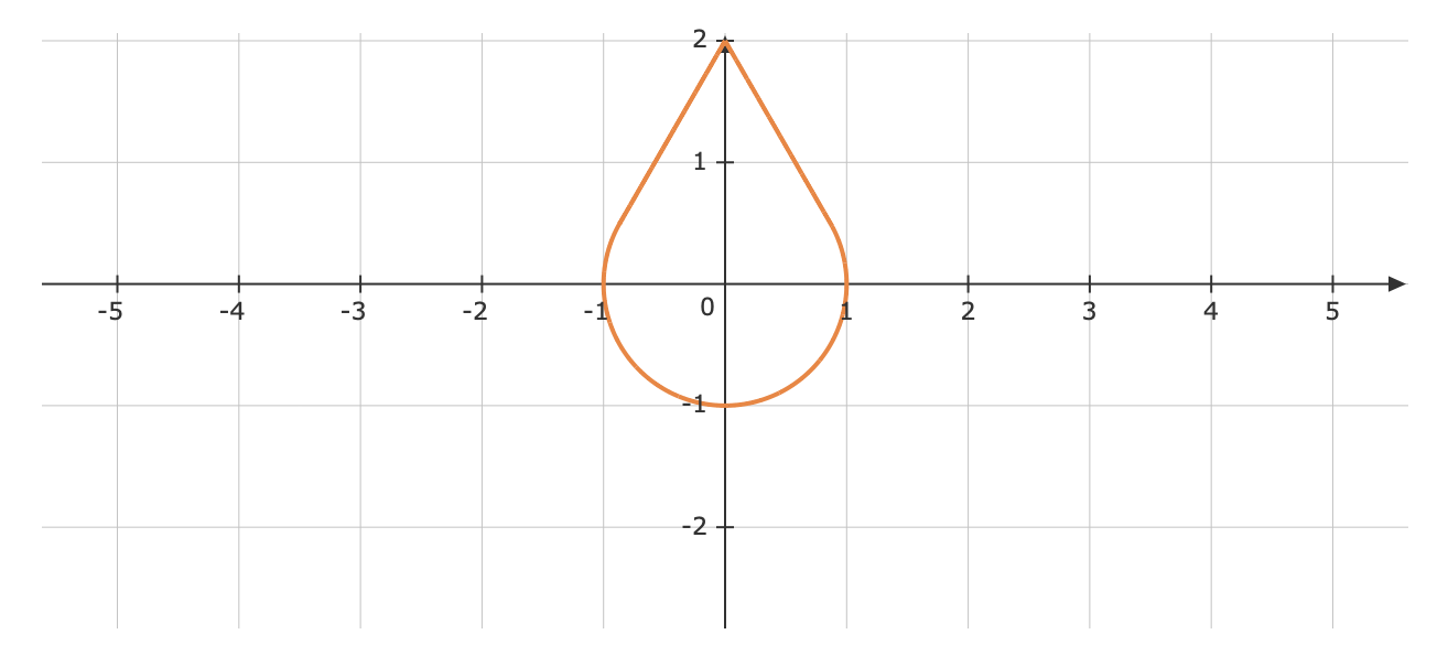
Figure 1:

For each quadratic boundary piece of $\tilde{Z}(S)$ the ideal generated by its equation and the equation of the ramification locus is radical. This computation was not performed modulo the Plücker relations though (but it seems not to be important).

3 Proving non-uniqueness

Due to the pole structure condition, the difference of any two forms satisfying all the properties of the canonical form is a holomorphic form. Covnersely, if $f$ satisfies all the propeties of the canonical form and $g$ is a global holomorphic form on the ambient variety $X$, then $f+g$ also satisfies the properites of the canonical form. Therefore, non-uniqueness of the canonical form is equivalent to existence of non-constant global holomorphic forms on $X$.

The canonical bundle of $\text{Gr}(2,6)$ is $\mathcal{O}(-6)$. By adjunction formula, the canonical bundle of the quartic ramification locus $R$ is $\mathcal{O}(-6+4)=\mathcal{O}(-2)$ (assuming the ramification locus is smooth; in the previous section we saw that this might not be the case). Assuming global sections $H^{0}(\mathbb{P}^{14},\mathcal{O}(-2))$ map surjectively onto $H^{0}(R,\mathcal{O}(-2))$, the bundle $\mathcal{O}(-2)$ still has no nonconstant global sections. However, one could intersect $R$ with quadratic boundary pieces $\tilde{Z}(S_{i})$. Assuming the intersection $R\cap\overline{\tilde{Z}(S_{i})}\cap\overline{\tilde{Z}(S_{j})}$ is smooth (which again seems to not be the case), its canonical bundle is $\mathcal{O}(2)$, which has nonconstant global sections. If this intersection contains a point in $\tilde{Z}(S)$, we are done. However, the singularities of this intersection might change the calculation and still eliminate the existence of global holomorphic forms. This would require intersecting $R$ with more quadratic pieces, reducing the chances that there is a point in $\tilde{Z}(S)$ in this intersection.

The positroid cell $S$ has $12$ codimension one boundary cells and $62$ codimension two boundary cells. All $12$ codimension one cells are mapped to the boundary of the Grasstope $\tilde{Z}(S)$, with $8$ of them having quadratic images and $4$ having linear images. Note that $58$ out of $62$ codimension two boundary cells can be obtained by intersecting two codimension one cells with quadratic images. This is a good indication that some of the images of these $58$ cells intersects the quartic fold. It is, however, still not clear how to prove this.

4 Images of lower-dimensional positroid strata and the ramification locus

Using the Mathematica package Positroids.m [jacob], we analyse the positroid stratification of $S$ and the intersections of images of positroid strata under the map $\tilde{Z}$ with the ramification locus. It turns out that all of one-dimensional positroid subcells of $S$ are entirely mapped to the ramification locus. In dimensions from 2 to 5, we have been able to find subcells that are mapped to the ramification locus and subcells whose images are not contained in the ramification locus but are also not disjoint from it (none of the subcells’ images are disjoint from the ramification locus since images of all the one-dimensional cells are contained in it). We have so far not been able to find a six-dimensional subcell that is mapped to the ramification locus (it seems highly likely that there are no such cells) and it is clear that none of the seven-dimensional subcells are mapped to the ramification locus. The five-dimensional subcell that we know is mapped to the ramification locus is given by the non-vanishing of the following Plücker coordinates: $p_{13},p_{14},p_{15},p_{16},p_{17},p_{18}$. Note that the image of this cell is four-dimensional.

We verify containment in the ramification locus as follows. First, we parametrise the cell in $\text{Gr}(2,8)_{\geq 0}$. The one mentioned above can be parametised as follows:

$$\begin{pmatrix}1&0&0&0&0&0&0&0\\ 0&0&a&b&c&d&e&1\end{pmatrix}$$

for $a,b,c,d,e\geq 0$. We then map the cell to $\text{Gr}(2,6)$ using the matrix $Z$. The image is the following parametrised set:

$$\begin{pmatrix}1&0&0&0&0&0\\ -6-e&5+e&-4+a-e&3+b+e&-2+c-e&1+d+e\end{pmatrix}.$$

The only nonzero Plücker coordinates on this set are $p_{12},p_{13},p_{14},p_{15},p_{16}$. The defining polynomial of the ramification locus does not contain a monomial that only contains these variables, so it has to vanish.

We would now like to show that the image of this cell appears as a face of the algebraic boundary of $\tilde{Z}(S)$. We know that the image of the following 7-subcell is mapped to a boundary divisor:

$$\begin{pmatrix}1&a&b&bd&be&bf&0&0\\ 0&0&c&cd&ce&cf&g&1\end{pmatrix}.$$

The corresponding boundary divisor is the parametrized as follows

$$\begin{pmatrix}1&a&b&bd&be&bf\\ -6-g&5+g&-4+c-g&3+cd+g&-2+ce-g&1+cf+g\end{pmatrix}.$$

The semialgebraic set $A$ inside this divisor which is the image of the positroid 7-cell is recovered by setting all the parameters to be real and non-negative. Setting $b=0$ gives a boundary piece of this set. However, this piece is $5$-dimensional, so it not a facet of the algebraic boundary. Now, it is either a face of codimension 2 (that is a facet of a facet of $A$ or directly a part of a lower-dimensional irreducible component of the algebraic boundary of $A$) or it intersects the interior of some facet of $A$. It is not immediately clear to me which of these two situations happens. Now, futher setting $a=0$, we recover a facet of this $5$-fold, which is contained in the ramification. Checking that this arises as a face of $\tilde{Z}(S)$ is now reduced to checking that the 5-fold is a face of $A$. A possible proof that the $5$-fold is a face might go as follows: all facets of $A$ arise as images of the boundary $6$-cells upstairs, and if the $5$-fold is not a face, it intersects (or even lies almost entirely in) the interior of a facet. Thus, if the 5-fold is not a face, a generic (or maybe not generic but belonging to a large set) point in its "real positive part" will have a preimage in a different $6$-cell (or even its interior). One can see whether this is true numerically but not prove this numerically.

5 Why things are hard

As mentioned in the previous sections, proving that a (sufficiently nice) semialgebraic set along with an ambient variety is not a positive geometry can essentially be done in two ways, by demonstrating either non-uniqueness or non-existence of the canonical form either on the whole set or on one of its faces. We now describe why this is hard.

Demonstrating non-uniquness fails since Zariski closures of each face of the considered Grasstope are rational varieties. As for non-existence, one might use the fact that any rational top-form on $\mathbb{P}^{d}$ has degree $-d-1$. Then if some face of the Grasstope has too few components in the boundary (i.e. their degrees add up to less than $d+1$) or too many components in the residual arrangement (those define the degree of the numerator; the notion of the residual arrangement can be generalized naturally from polytopes to Grasstopes), it cannot be a positive geometry. It is straightforward to see that every face of the Grasstope has sufficiently many faces, so one has to analyze the residual arrangement. This is computationally difficult as it requires calculating primary decompositions of many ideals (often of fairly high degree) in the coordinate ring of $\text{Gr}(2,8)$, which has many variables.

6 Maybe it is a positive geometry after all?

Our research was motivated by the following observation from Thomas Lam: if the map $\tilde{Z}$ is 1-to-1 on a positroid cell, a natural candidate for the canonical form on the corresponding Grasstope is the pushforward of the canonical form on the positroid cell. In our example the map is 2-to-1 for some fibers and, because of the presence of the quartic fold, the pushforward of the form on the positroid cell cannot be the canonical form of the Grasstope: the resulting form would not have a pole along the fold. This absence of a natural candidate for the canonical form of our Grasstope made us wonder if it is a positive geometry at all. And our lack of success in showing that it is not made us think that it might be.

The preimage of the quartic fold is the ramification locus of the map $\tilde{Z}$, which is a (quadratic (?)) hypersurface in $\text{Gr}(2,8)$. This hypersurface splits the 4-mass box cell $S$ into two components. On each of these components $\tilde{Z}$ is generically 1-to-1 and both of them are mapped to the Grasstope $\tilde{Z}(S)$. So if these pieces of the positroid cell are positive geometries, one can hope that the pushforward of the canonical form on any of them gives the canonical form on the Grasstope. It should in principle be simpler to study pieces of positroid cells since it is known that positroid cells themselves are positive geometries. So one has some information about the boundary structure and the residual arrangement for free. It remains to understand how the slicing hypersurface affects both the residual arrangement and the boundary structure. In the following sections we study this question for the case when the slicing hypersurface is a hyperplane.

7 The current question

Question (in highest generality): given a positroid cell $S$ and a hypersurface $H$ in $\text{Gr}(k,n)$, are closures of connected components of $S\setminus H$ positive geometries?

For our particular case of $k=2$, $n=8$ and $H$ being quadratic the explicit computation is again very hard. So we start from considering simpler examples. Namely, we slice the positive Grassmannian $\text{Gr}_{\geq 0}(2,4)$ with special hyperplanes to gain some intuition of what happens.

Example 7.1.

Consider a line in $\mathbb{P}^{3}$ with Plücker coordinates $(q_{12},q_{13},q_{23},q_{14},q_{24},q_{34})$. Then all the lines that meet this line form a hyperplane in $\text{Gr}(2,4)$. This hyperplane is defined by the equation

$$p_{12}q_{34}-p_{13}q_{24}+p_{14}q_{23}+p_{23}q_{14}-p_{24}q_{13}+p_{34}q_{12}=0.$$

We will consider one such hyperplane $H$ coming from a positive line in $\mathbb{P}^{3}$, namely the one defined by the equation

$$4p_{12}-7p_{13}+3p_{14}+10p_{23}-6p_{24}+3p_{34}=0.$$

It splits $\text{Gr}_{\geq 0}(2,4)$ into two connected components.

We analyze how $H$ intersects the positive Grassmannian $\text{Gr}_{\geq 0}(2,4)$. For all codimension $1$ and $2$ postiroid cells the intersection is non-empty and does not contribute to the residual arrangement. In codimension 3, there are 4 lines $l_{1},l_{2},l_{3},l_{4}$ that intersect $H$ strictly outside the positve Grassmannian: they are defined by non-vanishing of the following Plücker coordinates: $\{p_{14},p_{34}\},\{p_{12},p_{14}\},\{p_{23},p_{34}\},\{p_{12},p_{23}\}$. These 4 lines define the residual arrangement for the first connected component of $\text{Gr}(2,4)_{\geq 0}\setminus H$ (we denote this component by $S_{1}$). There is a pencil of hyperplanes interpolating those line. The unique adjoint is then defined by the condition that the residues of the canonical form at the vertices of $S_{1}$ are $\pm 1$ similarly to the case of polypols [kohn2021adjoints]. For our particular example the adjoint is given by the equation $-7p_{13}-6p_{24}=0$ (and, more generally, for a hyperplane defined by the point $(q_{12},\ldots,q_{34})$, it is given by $-q_{24}p_{13}-q_{13}p_{24}=0$ (up to sign).

None of the $6$ vertices of $\text{Gr}_{\geq 0}(2,4)$ are on $H$. 4 of them (defined by non-vanishing of $p_{14}$, $p_{34}$, $p_{12}$, $p_{23}$) are on the lines $l_{1},l_{2},l_{3},l_{4}$. The remaining 2 (defined by non-vanishing of $p_{13}$ and $p_{24}$) contribute to the residual arrangement of the second connected component $S_{2}$ of $\text{Gr}(2,4)_{\geq 0}\setminus H$. This residual arrangement consists of $6$ points: the 2 vertices of $\text{Gr}_{\geq 0}(2,4)$ described above and the $4$ intersection points $l_{i}\cap H$ for $i=1,\ldots,4$. These $6$ points are not in general position, there is a unique hyperplane in $\mathbb{P}^{5}$ that interpolates all of them, namely

$$4p_{12}+3p_{14}+10p_{23}+3p_{34}=0.$$

This (up to scaling) is the adjoint for $S_{2}$, so it looks like $S_{2}$ is a positive geometry.

One can also ask whether $H\cap\text{Gr}_{\geq 0}(2,4)$ is a positive geometry. In this case the adjoint should live inside $H$, have codimension 1 there, and interpolate the 4 intersection points $l_{i}\cap H$ that form the residual arrangement. Again, there seems to be a pencil of such adjoints, and the unique one should be defined by the residue conditions.

Observation: $S_{1}$ and $S_{2}$ are analogues of simple polytopes: each codimension $i$ face is adjacent to at most $i$ faces of codimension $i-1$. This property is desirable when one discusses the adjoint, and is ensured by the fact that $H$ is defined by a totally positive line.

Observation: unlike for polytopes, the residual arrangement of $S_{i}$ does not necessarily have codimension 2. In principle, it might not even be equidimensional.

Next questions: What happens if you slice with more hyperplanes? What happens if you slice with a quadric? How does this generalize to higher-dimensional Grassmannians?

We will now investigate what happens for a general Plücker hyperplane $H_{l}$ defined by a line $l\in\text{Gr}_{>0}(2,4)$. As mentioned above, if $l$ has Plücker coordinates $(q_{12},q_{13},q_{23},q_{14},q_{24},q_{34})$, then $H_{l}$ is given by the equation

$$p_{12}q_{34}-p_{13}q_{24}+p_{14}q_{23}+p_{23}q_{14}-p_{24}q_{13}+p_{34}q_{12}=0.$$

If $l\in\text{Gr}_{>0}(2,4)$, this equation has exactly $4$ positive and $2$ negative terms. We will use the following simple observation in our analysis.

Observation. $H_{l}$ intersects a face $P$ of $\text{Gr}_{>0}(2,4)$ if and only if there are two Plücker coordinates that do not vanish on $P$ and that appear with different signs in the equation of $H_{l}$.

This observation implies three things:

1. Since every dimension $2$ face has at least three non-vanishing Plücker coordinates and just two Plücker coordinates appear with a negative sign in the equation of $H_{l}$, we have that $H_{l}$ intersects every dimension $2$ face.

2. Since every vertex has only one non-vanishing Plücker coordinate, none of the vertices lie on $H_{l}$.

3. Since the conditions $p_{13}\neq 0$ and $p_{24}\neq 0$ (and all other $p_{ij}=0$) do not define a face of $\text{Gr}_{\geq 0}(2,4)$, a one-dimensional face $P$ intersects $H_{l}$ if and only if either $p_{13}$ or $p_{24}$ does not vanish on $P$.

These three things, in turn, characterize the residual arrangements of the two pieces $S_{1}$ and $S_{2}$ into which $\text{Gr}_{>0}(2,4)$ is sliced by $H_{l}$. Firstly, there are $4$ one-dimensional faces of $\text{Gr}_{\geq 0}(2,4)$ that do not intersect $H_{l}$. Each of these must belong to one of the two residual arrangements. Since $H_{l}$ restricted to each of these faces is defined by an equation with positive coefficients, the 4 faces belong to a single residual arrangement. Among the 6 vertices of $\text{Gr}_{\geq 0}(2,4)$, $4$ lie on these lines (and therefore to the same side of $H_{l}$), and the remaining $2$ (one is given by $p_{13}\neq 0$ and the other by $p_{24}\neq 0$, the Plücker coordinates appearing in the equation of $H_{l}$ with a negative sign) are in a different residual arrangement. This second residual arrangement also contains the $4$ intersections points of $H_{l}$ and the $4$ lines from the first residual arrangement. Therefore, the first residual arrangement consists of the 4 lines defined by non-vanishing of the following Plücker coordinates: $\{p_{14},p_{34}\},\{p_{12},p_{14}\},\{p_{23},p_{34}\},\{p_{12},p_{23}\}$. The unique adjoint interpolating this arrangement and satisfying the residue requirements is given by $-q_{24}p_{13}-q_{13}p_{24}=0$. The other arrangement is given by $6$ points: $4$ of them span a $\mathbb{P}^{2}$ and the remaining $2$ span a line disjoint from this $\mathbb{P}^{2}$, so in total the $6$ points span a $\mathbb{P}^{4}$ inside a $\mathbb{P}^{5}$, that is, they define a unique hyperplane, which is the adjoint. The correct normalization of the coeffients of its equation is again given by the residue condition.

Conjecture. Let $H$ be a hyperplane in $\text{Gr}(k,n)$ given by the equation

$$\sum\limits_{I\in\binom{[n]}{k}}c_{I}p_{I}=0,$$

where $c_{I}\neq 0$ for all $I$. Suppose $H\cap\text{Gr}_{>0}(k,n)\neq\varnothing$. Define $\overline{c_{I}}:=\max{(c_{I},0)}$ and $\underline{c_{I}}:=\min{(c_{I},0)}$. Then $H$ cuts the positive Grassmannian $\text{Gr}_{\geq 0}(k,n)$ into two pieces, each of which is a positive geometry, with the numerators of their canonical forms given by the linear forms

$$\sum\limits_{I\in\binom{[n]}{k}}\overline{c_{I}}p_{I}\text{ and }\sum\limits_{I\in\binom{[n]}{k}}\underline{c_{I}}p_{I}.$$

Idea behind the conjecture. Having all $c_{I}\neq 0$ means that $H$ does not contain a vertex of $\text{Gr}_{\geq 0}(k,n)$. Let $S_{1}$ and $S_{2}$ be the pieces into which $\text{Gr}_{\geq 0}(k,n)$ is cut by $H$ ($H$ really cuts the positive Grassmannian by assumption) but I am not sure that there are always just two pieces. Let $V_{i}$ be the set of vertices of $\text{Gr}_{\geq 0}(k,n)$ that are in $S_{i}$. Vertices of $\text{Gr}_{\geq 0}(k,n)$ are indexed by $I\in\binom{[n]}{k}$: $v_{I}=\{p_{I}\neq 0,p_{J}=0\quad\forall J\neq I\}$. We have $v_{I}\in V_{1}$ if $c_{I}<0$ and $v_{I}\in V_{2}$ if $c_{I}>0$. Note that $V_{1}$ is in the residual arrangement of $S_{2}$ and $V_{2}$ is in the residual arrangement of $S_{1}$. Any hyperplane interpolating $V_{1}$ has an equation of the form

$$\sum\limits_{I\in\binom{[n]}{k}}b_{I}p_{I},$$

where $b_{I}=0$ if $v_{I}\in V_{1}$. An analoguous description holds for hyperplanes interpolating $V_{2}$. The non-zero coefficients $b_{I}$ in the equation of the adjoint should be determined to be equal to $c_{I}$ either by the residue conditions or by additional components of the residual arrangement lying on $H$ (but showing this might be tricky for arbitrary $k$ and $n$).

The intersection of the residual arrangement $\mathcal{R}_{1}$ of $S_{1}$ with $H$ should be in the residual arrangement $\mathcal{R}_{2}$ of $S_{2}$. In particular, the intersection of $H$ and the linear space spanned by $\mathcal{R}_{1}$ should be interpolated by the adjoint of $\mathcal{R}_{2}$ and vice versa.

”Proof” We will ”prove” a simplified version of this conjecture.

First simplification. We assume that $H$ cuts all facets of $\text{Gr}(k,n)$. Since each facet is given by the vanishing of a single Plücker coordinate, this should be true when the equation of $H$ has at least two terms of each sign. One still needs to check that the Plücker relations do not affect this. If this is not true, at least one of the resulting pieces will have too few facets to have a canonical form.

Second simplification/assumption. We assume that $H$ really cuts $\text{Gr}_{\geq 0}(k,n)$ into two components, and not more. I currently have no idea how to check this (and even if this is true at all). It is somewhat hard to believe that a hyperplane cutting all the facets will only give two connected components. On second thought, the argument below does not depend on this assumption, one can define a positive part of $\text{Gr}_{\geq 0}(k,n)$ with respect to a hyperplane $H$ and not care about its connectedness as a topological space.

Let $S_{1}$ and $S_{2}$ be the pieces into which $\text{Gr}_{\geq 0}(k,n)$ is cut by $H$. We will now describe the residual arrangements $\mathcal{R}_{1}$ and $\mathcal{R}_{2}$ of $S_{1}$ and $S_{2}$, respectively. By the first assumption, each facet of $\text{Gr}_{\geq 0}(k,n)$ contributes a facet to both $S_{1}$ and $S_{2}$. The residual arrangement $\mathcal{R}_{i}$ consists of two parts. The first one (we denote it $\mathcal{R}^{G}_{i}$) consists of the intersections of facet hyperplanes of $\text{Gr}_{\geq 0}(k,n)$ that do not give a face of $S_{i}$. The second one (we denote in $\mathcal{R}^{H}_{i}$) consists of the intersections of $H$ with some of the facet hyperplanes of $\text{Gr}_{\geq 0}(k,n)$ that do not give a face of $S_{i}$. Since $c_{I}\neq 0$ for all $I$ by assumption, $H$ does not contain any vertex of $\text{Gr}_{\geq 0}(k,n)$. This means that each vertex of $\text{Gr}_{\geq 0}(k,n)$ is either in $\mathcal{R}^{G}_{1}$ or in $\mathcal{R}^{G}_{2}$. More precisely, $v_{I}\in\mathcal{R}^{G}_{1}$ if $c_{I}<0$ and $v_{I}\in\mathcal{R}^{G}_{2}$ if $c_{I}>0$. Note that if for two vertices $v$ and $w$ connected by an edge of $\text{Gr}_{\geq 0}(k,n)$ we have $v\in\mathcal{R}^{G}_{1}$ and $w\in\mathcal{R}^{G}_{2}$, then the edge of $\text{Gr}_{\geq 0}(k,n)$ between them contributes an edge to both $S_{1}$ and $S_{2}$, and is in none of the residual arrangements. This means that the span of $\mathcal{R}^{G}_{i}$ is equal to the span of vertices of $\text{Gr}_{\geq 0}(k,n)$ in $\mathcal{R}^{G}_{i}$.

We now turn to characterizing $\mathcal{R}^{H}_{i}$. If $F$ is a face of $\text{Gr}_{\geq 0}(k,n)$ that contributes a face to both $S_{1}$ and $S_{2}$, then it has to intersect $H$ inside $\text{Gr}_{\geq 0}(k,n)$, and therefore $F\cap H$ does not contribute to either of the residual arrangements. If $F$ only contributes a face to $S_{1}$, then it is in $\mathcal{R}^{G}_{2}$ and the hyperplane spanned by $F$ intersects $H$ outside of $\text{Gr}_{\geq 0}(k,n)$. This intersection is therefore in $\mathcal{R}^{H}_{1}$. If $F$ only contributes a face to $S_{2}$, then it already is in $\mathcal{R}^{G}_{1}$ and only contributes a lower-dimensional piece to $\mathcal{R}^{H}_{1}$. Thus, one can see that $\mathrm{span}(\mathcal{R}^{H}_{1})=\mathrm{span}(H\cap\mathcal{R}^{G}_{2})$ and, symmetrically, $\mathrm{span}(\mathcal{R}^{H}_{2})=\mathrm{span}(H\cap\mathcal{R}^{G}_{1})$. Since $\mathcal{R}_{i}=\mathcal{R}_{i}^{G}\cup\mathcal{R}_{i}^{H}$, we now can describe the span of $\mathcal{R}_{i}$, which is a projective space.

Any hyperplane interpolating $\mathcal{R}_{1}$ has an equation of the form

$$\sum\limits_{I\in\binom{[n]}{k}}b_{I}p_{I},$$

where $b_{I}=0$ if $v_{I}\in\mathcal{R}_{1}$. The residue conditions at the vertices $v_{I}\in S_{1}$ for the adjoint imply $b_{I}=c_{I}$ if $v_{I}\in S_{1}$, which defines a unique hyperplane $A$. The span of $H\cap\mathcal{R}^{G}_{2}$ is contained in $H\cap\mathrm{span}(\{v_{I}|c_{I}<0\})$. The ideal of this latter intersection contains the defining polynomial $\sum c_{I}p_{I}$ of $H$ as well as any linear form

$$\sum\limits_{I\in\binom{[n]}{k}}b_{I}p_{I},$$

where $b_{I}=0$ if $v_{I}\in S_{1}$. In particular, by setting $b_{I}=c_{I}$ for $v_{I}\in\mathcal{R}_{1}$ and subtracting the resulting form from $\sum c_{I}p_{I}$, we get the defining equation of $A$. Thus, $A$ interpolates $\mathcal{R}^{H}_{1}$. It therefore interpolates the whole residual arrangement $\mathcal{R}_{1}$ and is the adjoint of $S_{1}$. The canonical form of $S_{1}$ is then given by

$$\Omega(S_{1})=\dfrac{A}{p_{1\ldots k}p_{2\ldots k+1}\ldots p_{n1\ldots k-1}H}.$$

The proof for $S_{2}$ is analogous.

We now investigate the situation in which our first simplifying assumption does not hold, namely when there is a facet $F$ of $\text{Gr}_{\geq 0}(k,n)$ that is disjoint from $H$. Arguably the simplest example is given by the hyperplane $H$ defined by

$$-p_{12}+p_{13}+p_{14}+p_{23}+p_{24}+p_{34}=0$$

in $\text{Gr}_{\geq 0}(2,4)$. The facet of $\text{Gr}_{\geq 0}(2,4)$ given by $p_{12}=0$ is then disjoint from $H$. This means that $H$ cuts $\text{Gr}_{\geq 0}(2,4)$ into two (again: really two?) parts. One of them (say, $S_{1}$) has $5$ facets (the $4$ facets of the positive Grassmannian and $H$), while the other one (say, $S_{2}$) only has $4$ facets (the 3 facets of $\text{Gr}_{\geq 0}(2,4)$ intersected by $H$ and $H$ itself). The latter piece $S_{2}$ is then a simplex-like positive geometry, there is no adjoint. The former piece $S_{1}$ has the canonical form with the adjoint given by $p_{12}=0$. So in this case the conjecture only works partially: if there is an adjoint, one can recover it by using the conjecture, but it cannot predict if there is no adjoint at all.

Question: for larger $k$ and $n$, can $H$ cut ”too few” facets? Looking only at the linear equations, it looks like it is impossible, either $H$ cuts no facets (if all the coefficients of $H$ have the same sign), or it avoids at most one of them (this happens if there is just one negative coefficient). But do the Plücker relations really not change this?

8 Two hyperplanes

In this section we consider a piece of $\text{Gr}_{\geq 0}(2,4)$ bounded by two hyperplanes $H_{1}$ and $H_{2}$ and show that this is in general not a positive geometry.

We condsider the hyperplanes $H_{1}$ and $H_{2}$ defined by the linear forms

$$h_{1}(p)=p_{12}-p_{13}+p_{23}-p_{14}+p_{24}-p_{34}$$

and

$$h_{2}(p)=p_{12}+2p_{13}-p_{23}-2p_{14}+2p_{24}+p_{34}$$

respectively. We consider a subset $S$ of $\text{Gr}_{\geq 0}(2,4)$ ”defined” by the conditions $h_{1}(p)\geq 0$ and $h_{2}(p)\geq 0$. More precisely, we consider the region where $h_{1}$, $h_{2}$ and the linear forms $p_{12},p_{14},p_{23},p_{34}$ defining the facets of $\text{Gr}_{\geq 0}(2,4)$ have the same sign. The residual arrangement $\mathcal{R}$ of $S$ in $\text{Gr}(2,4)$ consists of the following subspaces:

$$p_{12}=p_{23}=p_{24}=0,$$

$$p_{14}=p_{23}=p_{13}+p_{34}=p_{12}+p_{24}=0,$$

$$p_{34}=p_{23}+p_{24}=p_{13}+p_{14}=p_{12}=0,$$

$$p_{14}=p_{23}=p_{12}+2p_{13}+2p_{24}+p_{34}=p_{13}p_{24}+2p_{13}p_{34}+2p_{24}p_{34}+p_{34}^{2}=0,$$

$$p_{13}=p_{14}=p_{34}=h_{1}(p)=0,$$

$$p_{13}=p_{23}=p_{24}=p_{34}=h_{1}(p)=0,$$

$$p_{12}=p_{13}=p_{14}=p_{24}=p_{34}=0.$$

Since we are dealing with an arrangement of 6 hyperplanes in $\text{Gr}(2,4)$, the adjoint interpolating the residual arrangement should be a quadric. There is indeed a two-dimensional family of quadrics interpolating $\mathcal{R}$. These are of the form

$$\alpha p_{13}p_{23}+\alpha p_{14}p_{23}+\beta p_{13}p_{24}-\beta p_{12}p_{34}+\gamma p_{23}p_{24}=0.$$

If $S$ is a positive geometry, the canonical form is of the form

$$f(p)=\dfrac{(\alpha p_{13}p_{23}+\alpha p_{14}p_{23}+\beta p_{13}p_{24}-\beta p_{12}p_{34}+\gamma p_{23}p_{24})dp_{12}\wedge dp_{23}\wedge dp_{34}\wedge dp_{14}}{p_{12}p_{23}p_{34}p_{14}(p_{12}-p_{13}+p_{23}-p_{14}+p_{24}-p_{34})(p_{12}+2p_{13}-p_{23}-2p_{14}+2p_{24}+p_{34})}.$$

Now iteratively taking residues at $p_{12}=0$, $p_{23}=0\And p_{13}=0$, $p_{34}=0$, we get the form

$$\dfrac{\beta p_{24}^{2}dp_{14}}{2(p_{24}-p_{14})^{2}},$$

which has a double pole at the point $p_{14}=p_{24}\neq 0$ and $p_{12}=p_{13}=p_{23}=p_{34}=0$. This point is a vertex of $S$, and therefore $S$ cannot be a positive geometry.

This double pole is a consequence of non-genericity of $H_{1}$ and $H_{2}$. A genericity assumption that is supposed to ensure that there are no double poles is that the $2\times 6$ matrix of coefficients of the linear forms $h_{1}$ and $h_{2}$ does not have a zero maximal minor.

The next natural question to ask is what happens when $H_{1}$ and $H_{2}$ are generic enough. Is there still a piece of the positive Grassmannian that sees all $6$ hyperplanes as facets? If so, is it a positive geometry?

We turn to the case of two somewhat more generic hyperplanes. These are defined by equations

$$l_{1}(p)=5p_{12}-p_{13}+2p_{23}+4p_{14}-3p_{24}+2p_{34}=0$$

and

$$l_{2}(p)=4p_{12}+3p_{13}+p_{23}-p_{14}+5p_{24}-2p_{34}=0.$$

The residual arrangement consists of the following components (5 points, 3 lines and one codimension two component):

$$p_{12}=p_{13}=p_{23}=p_{24}=0,$$

$$p_{12}=p_{13}=p_{14}=p_{23}=p_{34}=0,$$

$$p_{12}=p_{14}=p_{23}=p_{24}=p_{34}=0,$$

$$p_{13}=p_{14}=p_{34}=h_{2}(p)=0,$$

$$p_{14}=p_{24}=p_{34}=h_{2}(p)=0,$$

$$p_{13}=p_{23}=p_{24}=p_{34}=h_{1}(p)=0,$$

$$p_{12}=p_{13}=p_{14}=p_{24}=h_{1}(p)=0,$$

$$p_{13}=p_{14}=p_{24}=p_{34}=h_{1}(p)=0,$$

$$h_{1}(p)=h_{2}(p)=0.$$

There is a unique (up to scaling) quadric vanishing on this arrangement. This gives a unique candidate for the canonical form of this geometry.

$4p_{12}+3p_{13}+p_{23}+5p_{24}=0$ contains the three lines.

Let us try to see the unique quadric (modulo the Grassmannian) theoretically. Then we first record the incidences between the different components of this residual arrangement and their spans. Of the three lines $L_{1},L_{2},L_{3}$ in the residual arrangement $L_{2}$ and $L_{3}$ meet in a point. All three together span a $\mathbb{P}^{4}$. The quadric surface $S$ intersects the two lines $L_{2}$ and $L_{3}$. The five points span a $\mathbb{P}^{4}$, and are in linear general position with all the other components.

Let $\Gamma$ be the whole residual arrangement, and $\Gamma_{0}=S\cup L_{2}\cup L_{3}.$ Then $\Gamma_{0}$ is contained in a hyperplane $H_{0}$ that intersects $L_{1}$ in a point. Let $\Gamma_{1}=\Gamma\setminus\Gamma_{0}$, it is the union of the five isolated points and the line $L_{1}$, and it is not contained in a hyperplane. Consider now short exact sequence of ideal sheaves

$$0\to I_{\Gamma_{1}}(1)\to I_{\Gamma}(2)\to I_{\Gamma\cap H_{0},H_{0}}(2)\to 0,$$

where the second map is multiplication by $H_{0}$. Taking cohomology, the first sheaf has $h^{0}=0,h^{1}=1$ as can be seen from the cohomology of ideal sequence

$$0\to I_{\Gamma_{1}}(1)\to{\mathcal{O}}_{\bf{P}^{5}}(1)\to{\mathcal{O}}_{\Gamma_{1}}(1)\to 0),$$

when noticing that there is no global section in the left ideal sheaf, since $\Gamma_{1}$ is not contained in a hyperplane. On the right hand side, $h^{0}(I_{\Gamma\cap H_{0},H_{0}}(2))=2$; there is a pencil of quadrics in $H_{0}$ that contain $\Gamma\cap H_{0}=\Gamma_{0}\cup(L_{1}\cap H_{0}),$ since $S\cup L_{2}\cup L_{3}$ in $3$ quadrics inside $H_{0}$, while $L_{1}\cap H_{0}$ is contained in $2$ of them. We conclude that the residual arrangement is contained in (at least) $1$ quadric and at most $2$ quadrics (one modulo the Grassmann quadric). The $2$ would be a closed condition (that seems always to be the case…)

Example 8.1.

One sees that the residual arrangement depends greatly on the signs of the coefficients of the defining equations of the two additional hyperplanes. For instance, consider the hyperplanes defined by

$$h_{1}(p)=-p_{12}+3p_{13}+2p_{23}+2p_{14}+p_{24}-5p_{34}=0,$$

$$h_{2}(p)=p_{12}+p_{13}-p_{23}-3p_{14}+2p_{24}+2p_{34}=0.$$

The residual arrangement now consists of 3 lines, 2 conics and 2 points:

$$p_{14}=p_{23}=h_{2}(p)=p_{12}p_{34}-p_{13}p_{24}=0,$$

$$p_{12}=p_{34}=h_{1}(p)=p_{14}p_{23}-p_{13}p_{24}=0,$$

$$p_{13}=p_{14}=p_{34}=h_{1}(p)=h_{2}(p)=0,$$

$$p_{14}=p_{24}=p_{34}=h_{1}(p)=h_{2}(p)=0,$$

$$p_{12}=p_{13}=p_{23}=p_{24}=0,$$

$$p_{13}=p_{23}=p_{24}=p_{34}=0,$$

$$p_{12}=p_{13}=p_{14}=p_{24}=0.$$

There still is a unique adjoint.

Let us try to see this theoretically. Then we first record the incidences between the different components of this residual arrangement and their spans. The three lines $L_{1},L_{2},L_{3}$ in the residual arrangement have two points of pairwise intersections, and together span a $\mathbb{P}^{3}$. The two conics $C_{1}$ and $C_{2}$ are disjoint from the lines and from each other, and each conic spans a $\mathbb{P}^{2}$. Finally, the two points $Q_{1},Q_{2}$ span a line that is disjoint from all other components of the arrangement.

Let $\Gamma$ be the whole residual arrangement, and $\Gamma_{0}$ the part consisting of one of the isolated points, say $Q_{1}$ and the three lines. Then $\Gamma_{0}$ is contained in a hyperplane $H_{0}$ that intersects each of the conics $C_{1}$ and $C_{2}$ in two points. Let $\Gamma_{1}=\Gamma\setminus\Gamma_{0}$, it is $C_{1}\cup C_{2}\cup Q_{2}$ and is not contained in a hyperplane. Consider now short exact sequence of ideal sheaves

$$0\to I_{\Gamma_{1}}(1)\to I_{\Gamma}(2)\to I_{\Gamma\cap H_{0},H_{0}}(2)\to 0,$$

where the second map is multiplication by $H_{0}$. Taking cohomology, the first sheaf has $h^{0}=0,h^{1}=1$ as can be seen from the cohomology of ideal sequence

$$0\to I_{\Gamma_{1}}(1)\to{\mathcal{O}}_{\bf{P}^{5}}(1)\to{\mathcal{O}}_{\Gamma_{1}}(1)\to 0),$$

when noticing that there is no global section in the left ideal sheaf, since $\Gamma_{1}$ is not contained in a hyperplane. On the right hand side, $h^{0}(I_{\Gamma\cap H_{0},H_{0}}(2))=3$; there is a pencil of quadrics that contain $\Gamma\cap H_{0}=\Gamma_{0}\cup(C_{1}\cup C_{2})\cap H_{0},$ since the three lines lie in $8$ quadrics inside $H_{0}$, while $Q_{1}$ and $(C_{1}\cup C_{2})\cap H_{0},$ are contained in $3$ of them. (exactly three as long as these last points impose independent conditions). We conclude that the residual arrangement is contained in (at least) $2$ quadrics (one modulo the Grassmann quadric) and at most $3$ quadrics. The $2$ would be an open condition (possibly empty).

Example 8.2.

Now, consider two hyperplanes

$$h_{1}(p)=p_{12}-3p_{13}-2p_{23}+2p_{14}+p_{24}+5p_{34}=0,$$

$$h_{2}(p)=p_{12}+p_{13}-p_{23}+3p_{14}-2p_{24}+2p_{34}=0.$$

Along with the 4 positroid hyperplanes, these form a simple hyperplane arrangement. The residual arrangement is given by 8 lines and 1 conic.

$$p_{23}=h_{1}(p)=h_{2}(p)=p_{12}p_{34}-p_{13}p_{24}=0,$$

$$p_{12}=p_{13}=p_{23}=h_{1}(p)=0,$$

$$p_{12}=p_{23}=p_{24}=h_{2}(p)=0,$$

$$p_{23}=p_{24}=p_{34}=h_{2}(p)=0,$$

$$p_{13}=p_{23}=p_{34}=h_{1}(p)=0,$$

$$p_{12}=p_{13}=p_{14}=h_{1}(p)=0,$$

$$p_{14}=p_{24}=p_{34}=h_{2}(p)=0,$$

$$p_{12}=p_{14}=p_{24}=p_{34}=0,$$

$$p_{12}=p_{13}=p_{14}=p_{34}=0.$$

Now, unlike in the previous examples, the adjoint is not unique. Modulo the Plücker relation, there is a pencil of quadrics interpolating the residual arrangement. The pencil is spanned by $p_{14}p_{23}$ and $p_{12}^{2}+p_{12}p_{13}+5p_{12}p_{14}+2p_{13}p_{14}+6p_{14}^{2}-p_{12}p_{23}+p_{12}p_{24}+3p_{14}p_{24}+2p_{12}p_{34}+5p_{13}p_{34}+19p_{14}p_{34}-4p_{23}p_{34}+2p_{24}p_{34}+10p_{34}^{2}$.

The 1-skeleton of the boundary of the region $\text{Gr}_{\geq 0}(2,4)\cap\{h_{1}\geq 0\}\cap\{h_{2}\geq 0\}$ is connected. It contains 27 one-dimensional irreducible components: 7 conics and 20 lines. Out of the 20 lines, 4 are only contained in 2 facet hyperplanes, while the remaining 16 are contained in 3 facet hyperplanes and come in pairs, one pair per triplet of hyperplanes whose intersection with the Grassmannian is not an irreducible conic. Each one-dimensional component contains 2 vertices of the region, and in total the region has 14 vertices. Each linear one-dimensional boundary component should contain 2 vertices from the residual arrangement, and each conic component should contain 4 residual vertices (CHECK).

We now address Question 8.8 for this example. The two Schubert hyperplanes contained in the pencil spanned by $h_{1}$ and $h_{2}$ are

$$s_{1}(p)=(5-2\sqrt{3})p_{12}+(1-2\sqrt{3})p_{13}-(6-2\sqrt{3})p_{23}+(14-6\sqrt{3})p_{14}-(5-4\sqrt{3})p_{24}+(13-4\sqrt{3})p_{34}=0,$$

$$s_{2}(p)=(5+2\sqrt{3})p_{12}+(1+2\sqrt{3})p_{13}-(6+2\sqrt{3})p_{23}+(14+6\sqrt{3})p_{14}-(5+4\sqrt{3})p_{24}+(13+4\sqrt{3})p_{34}=0.$$

The residual arrangement of $\text{Gr}_{\geq 0}(2,4)\cap\{s_{1}=0\}\cap\{s_{2}=0\}$ has the same structure as that of $\text{Gr}_{\geq 0}(2,4)\cap\{h_{1}=0\}\cap\{h_{2}=0\}$: there is the same number of components of each degree and dimension. Moreover, the equations for these components are the same up to replacing $h_{i}$ with $s_{i}$. The family of adjoints should therefore also be two-dimensional (since these hyperplanes are not defined over $\mathbb{Q}$, I could not compute this family explicitly). Note that the signs of coefficients of $s_{1}$ and $s_{2}$ are the same as those of $h_{1}$ and $h_{2}$.

Example 8.3.

We now consider two Schubert hyperplanes defined over $\mathbb{Q}$. The coefficient vectors of these hyperplanes have the same sign patterns as in the previous example. The hyperplanes are

$$h_{1}=p_{12}-3p_{13}-p_{23}+8p_{14}+2p_{24}+2p_{34}=0.$$

$$h_{2}=2p_{12}+p_{13}-5p_{23}+p_{14}-3p_{24}+p_{34}=0,$$

The residual arrangement is still given by 8 lines and 1 conic. These components, however, come from slightly different positroid cells than in the previous examples. Namely, the equations for the components of the residual arrangement are

$$p_{23}=h_{1}(p)=h_{2}(p)=p_{12}p_{34}-p_{13}p_{24}=0,$$

$$p_{12}=p_{13}=p_{23}=h_{1}(p)=0,$$

$$p_{12}=p_{23}=p_{24}=h_{2}(p)=0,$$

$$p_{23}=p_{24}=p_{34}=h_{2}(p)=0,$$

$$p_{13}=p_{23}=p_{34}=h_{1}(p)=0,$$

$$p_{12}=p_{13}=p_{14}=h_{1}(p)=0,$$

$$p_{13}=p_{14}=p_{34}=h_{1}(p)=0,$$

$$p_{12}=p_{14}=p_{24}=p_{34}=0,$$

$$p_{12}=p_{13}=p_{14}=p_{34}=0.$$

The sixth and the seventh equations are different from those in the previous example. The family of adjoints is again two-dimensional, and is spanned by $p_{13}p_{24}$ and $2p_{12}^{2}+p_{12}p_{13}+17p_{12}p_{14}+8p_{13}p_{14}+8p_{14}^{2}-2p_{12}p_{23}+4p_{12}p_{24}+2p_{14}p_{24}-2p_{12}p_{34}+2p_{13}p_{34}+10p_{14}p_{34}-p_{23}p_{34}+2p_{24}p_{34}+2p_{34}^{2}$. The monomial support of these generators is the same as of those in the previous example.

Example 8.4.

Let the hyperplanes $h_{1}$ and $h_{2}$ be as in the previous example. The region we are interested now is, however, given by $h_{1}\leq 0,h_{2}\geq 0$ inside $\text{Gr}_{\geq 0}(2,4)$. The residual arrangement in this case is not a curve, it has codimension (and dimension) 2 (but there is one one-dimensional component as well), and there are 6 components: four planes, one quadric surface, and one point. The equations are

$$h_{2}(p)=p_{23}=p_{12}p_{34}-p_{13}p_{24}=0,$$

$$p_{12}=p_{13}=p_{23}=0,$$

$$p_{13}=p_{23}=p_{34}=0,$$

$$p_{12}=p_{13}=p_{14}=0,$$

$$p_{13}=p_{14}=p_{34}=0,$$

$$p_{12}=p_{14}=p_{24}=p_{34}=h_{1}(p)=0.$$

There is a pencil of adjoints spanned by $p_{13}p_{24}$ and $6p_{12}p_{13}+3p_{13}^{2}+3p_{13}p_{14}+p_{13}p_{23}-9p_{12}p_{34}+3p_{13}p_{34}$.

Now suppose we look at $h_{1}\geq 0,h_{2}\leq 0$. The residual arrangement consists of a quadric surface, two planes, one line, and three points:

$$h_{1}(p)=p_{23}=p_{12}p_{34}-p_{13}p_{24}=0,$$

$$p_{12}=p_{13}=p_{23}=0,$$

$$p_{23}=p_{24}=p_{34}=0,$$

$$p_{12}=p_{14}=p_{24}=p_{34}=0,$$

$$h_{1}(p)=h_{2}(p)=p_{12}=p_{13}=p_{14},$$

$$h_{1}(p)=h_{2}(p)=p_{12}=p_{14}=p_{24}=p_{34},$$

$$p_{12}=p_{13}=p_{14}=p_{34}=h_{2}(p)=0.$$

There is a pencil of adjoints. It is spanned by $p_{13}p_{24}$ and $3p_{12}p_{23}+3p_{12}p_{24}+24p_{14}p_{24}+10p_{23}p_{24}+6p_{24}^{2}-9p_{12}p_{34}+9p_{23}p_{34}+6p_{24}p_{34}$.

Finally, consider $h_{1}\leq 0$ and $h_{2}\leq 0$. The hyperplane $p_{23}=0$ now does not make a facet of this region. There is just five facets. The residual arrangement consists of two lines and a point:

$$h_{2}(p)=p_{12}=p_{13}=p_{14}=0,$$

$$h_{2}(p)=p_{13}=p_{14}=p_{34}=0,$$

$$h_{1}(p)=p_{12}=p_{14}=p_{24}=p_{34}=0.$$

The family of adjoints is two-dimensional, and the adjoints are now linear. It is spanned by the defining polynomial of a facet hyperplane $p_{14}$ and the linear form $2p_{12}-15p_{13}-5p_{23}-3p_{24}+p_{34}$.

Observation. In the above example the “extra” adjoint is a term $p_{13}p_{24}$ in the Plücker relation. This might mean this is, in a certain sense, a non-generic situation.

The examples above lead us to the following set of questions and conjectures.

Conjecture 8.5.

As long as the hyperplane arrangement given by the positroid hyerplanes and the two additional hyperplanes is simple, the dimension of the family of adjoints of the positive region of this arrangement inside $\text{Gr}(2,4)$ (and maybe even the monomial support of the adjoints) depends only on the vectors of signs of coefficients of $h_{1}$ and $h_{2}$, that is, on oriented matroid strata of $h_{1}$ and $h_{2}$ inside $\text{Gr}(4,5)\cong\mathbb{P}^{5}$ (the coefficients are assumed to be generic though). This probably is true for arbitrary $k$ and $n$ in $\text{Gr}(k,n)$ but should certainly first be understood for $\text{Gr}(2,4)$. A complete classification of "good" strata for arbitrary Grassmannians is obviously completely out of reach. On second thought, when it comes to the actual residual arrangement, it might be more complicated, absolute values of the coefficients might also play a role in determining the number of its components.

Question 8.6.

Which matroid strata give a unique adjoint? Is a classification feasible at least in the $\text{Gr}(2,4)$ case?

Question 8.7.

If the adjoint is not unique, do the residue conditions on the vertices of the region still give a unique canonical form? If so, what are the conditions for this to be true? How many "independent" residue conditions does one get? Is it equal to the number of connected (strongly connected) components of the region/of the 1-skeleton of the boundary?

ToDo: in the last example, there are 14 vertices. One should compute the residue at each of them in order to see explicitly how many independent conditions on the adjoint there are.

Question 8.8.

The two additional hyperplanes $h_{1}$ and $h_{2}$ span a pencil containing exactly two Schubert hyperplanes. What happens if one replaces $h_{1}$ and $h_{2}$ by these Schubert hyperplanes? It is simpler but still instructive?

8.1 Sign patterns and oriented matroids

We are studying the instersection of $\text{Gr}_{\geq 0}(2,4)$ with two half-spaces defined by $h_{1}(p)\geq 0$ and $h_{2}(p)\geq 0$. This positive region is bounded by six hyperplanes. The same six hyperplanes cut bound a positive region in $\mathbb{P}^{5}$, which is a polyhedron, and this polyhedron contains the original region. The residual arrangement of this polyhedron has pure codimension two. The six facet hyperplanes of the polyhedron are oriented (in a sense that a positive half-space is chosen for each of them), and define an oriented matroid. Each region of the hyperplane arrangement corresponds to a covector of this matroid, and is labeled by a sequence of six signs $-$, $+$ and $0$, depending on whether it lies in the positive/negative half-space w.r.t. $h_{i}$ or on $h_{i}$. The residual arrangement then consists of the regions with labels containing at least two zeros and at least one minus. The residual arrangement of the original region inside $\text{Gr}(2,4)$ is then obtained as the intersection of the residual arrangement of the polyhedron with $\text{Gr}(2,4)$. The matroid is essentially defined by the signs of the maximal minors of the matrix of coefficient vectors, so these are the signs that matter.

9 The associated polytope

Consider two hyperplanes in the Plücker space $\mathbb{P}^{5}$ given by the equations $h_{1}(p)=0$ and $h_{2}(p)=0$. We are interested in the region $S\subseteq\text{Gr}_{\geq 0}(2,4)$ defined by the inequalities $p_{ij}\geq 0$ for any Plücker coordinate $p_{ij}$ and $h_{1}(p)\geq 0$, $h_{2}(p)\geq 0$ and a single equation $p_{12}p_{34}-p_{13}p_{24}+p_{14}p_{23}=0$ defining $\text{Gr}(2,4)$. The linear inequalities should be projectively interpreted as follows: the product of any two linear forms is non-negative, that is, all linear forms have the same sign. If we drop the equation of $\text{Gr}(2,4)$, the remaining inequalities define a polytope in $\mathbb{P}^{5}$. We call it the associated polytope of $S$ and denote in by $\mathcal{P}_{S}$. We denote the residual arrangement of $S$ by $\mathcal{R}(S)$ and the residual arrangement of $\mathcal{P}_{S}$ by $\mathcal{R}(\mathcal{P}_{S})$.

Proposition 9.1.

Let $V$ be the variety in $\mathbb{P}^{5}$ defined by the vanishing of the Plücker monomials: $p_{12}p_{34}=p_{13}p_{24}=p_{14}p_{23}=0$. Assume that the facets of $S$ are given by $h_{1}=0$, $h_{2}=0$ and the positroid hyperplanes. Then $V\cap\mathcal{R}(S)=V\cap\mathcal{R}(\mathcal{P}_{S})$.

Proof 9.2.

The variety $V$ consists of the $8$ positroid planes in $\text{Gr}(2,4)$. In particular, each point of $V$ is contained in at least two positroid hyperplanes. Let $X$ be a component of $\mathcal{R}(\mathcal{P}_{S})$. Then, due to the observation above, $X\cap V$ is contained in the intersection of at least two facet hyperplanes of $S$. Moreover, we have $X\cap V\subseteq V\subseteq\text{Gr}(2,4)$. Therefore, since $X\cap V$ is equal to the intersection of a subset of the facet hyperplanes of $\mathcal{P}_{S}$, $X\cap V$ either is in $S$ or in $\mathcal{R}(S)$. Since, due to convexity, $X$ is disjoint from $\mathcal{P}_{S}$ and $S=\mathcal{P}_{S}\cap\text{Gr}(2,4)$, we conclude that $X\cap V$ is disjoint from $S$ and is therefore in $\mathcal{R}(S)$. Thus, $V\cap\mathcal{R}(\mathcal{P}_{S})\subseteq V\cap\mathcal{R}(S)$.

Conversely, let $Y$ be a component of $\mathcal{R}(S)$. Then $Y\cap V$ is contained in the intersection of facet hyperplanes of $S$. Each facet hyperplane of $S$ is also a facet hyperplane of $\mathcal{P}_{S}$, so $Y\cap V$ is either in $\mathcal{P}_{S}$ or in $\mathcal{R}(\mathcal{P}_{S})$. Since $S=\mathcal{P}_{S}\cap\text{Gr}(2,4)$ and $Y\cap V\subseteq V\subseteq\text{Gr}(2,4)$, $Y\cap V\not\subset S$, we conclude $Y\cap V\not\subset\mathcal{P}_{S}$ and thus $Y\cap V\subseteq\mathcal{R}(\mathcal{P}_{S})$. Thus, $V\cap\mathcal{R}(\mathcal{S})\subseteq V\cap\mathcal{R}(\mathcal{P}_{S})$.

Proposition 9.1 implies that modulo the ideal of $V$ any adjoint of $S$ is the same as the adjoint of $\mathcal{P}_{S}$. It remains to show that modulo this ideal there is just one adjoint of $S$. This would follow from showing that there is a unique quadric (modulo $I(V)$) interpolating $\mathcal{R}(S)\cap V=\mathcal{R}(\mathcal{P}_{S})\cap V$. This can be shown as follows, I think. If $\mathcal{P}_{S}$ is a simple polytope, there is a unique quadric interpolating it by [kohn2020projective]. Then there are the three quadrics generating $I(V)$. $I(V\cap\mathcal{R}(\mathcal{P}_{S}))=I(V)+I(\mathcal{R}(\mathcal{P}_{S}))$ and therefore has (at most?) $4$ quadrics. Now, $\mathcal{R}(S)$ contains $V\cap\mathcal{R}(\mathcal{P}_{S})$ and therefore any quadric interpolating $\mathcal{R}(S)$ interpolates $V\cap\mathcal{R}(\mathcal{P}_{S})$, and therefore is in the family generated by the four quadrics. Modulo $I(V)$ there is therefore at most one. The remaining question is why one always exists…

And here is an argument why one always exists under a mild genericity assumption (that is true for essentially the same reasons). Suppose the adjoint polynomial $\alpha_{\mathcal{P}}$ of $\mathcal{P}_{S}$ is not in the ideal $I(V)=\langle p_{12}p_{34},p_{13}p_{24},p_{14}p_{23}\rangle$. We have $I(\mathcal{P}_{S})=I(\mathcal{S})\ \mathrm{mod}\ I(V)$, so there has to be a quadric in $I(\mathcal{S})$ that is not in $I(V)$ if there is a quadric in $I(\mathcal{P}_{S})$ that is not in $I(V)$. It remains to verify the assumption that the unique adjoint polynomial $\alpha_{\mathcal{P}}$ of $\mathcal{P}_{S}$ does not vanish on $V$. Consider any pair of hyperplanes in the boundary of $\mathcal{P}_{S}$. Their common intersection is a $3$-space and the restriction of the polytope $\mathcal{P}_{S}$ to this $3$-space is a $3$-dimensional polytope with at most six facets. Since $\mathcal{P}_{S}$ is simple, so is this restriction. Therefore it has at least four facets. Its residual arrangement is contained in the residual arrangement of $\mathcal{P}_{S}$. In addition, if it has four or five facets, the residual arrangement of $\mathcal{P}_{S}$ contains two or one plane respectively, the restriction of the hyperplanes of $\mathcal{P}_{S}$ that do not contain any of the facets. The residual arrangement of the restricted polytope is otherwise empty when it has four facets, and a line and a point, if it has five facets. If it has six facets, the residual arrangement consists of three skew lines or the union of three lines that form a simple chain and two points whose span does not intersect any of the three lines (cf [kohn2020projective]. Now, if the adjoint $\alpha_{\mathcal{P}}$ already contains $V$, we argue that it cannot contain the residual arrangements in all the $3$-spaces of pairs of hyperplanes..

Discussion on August 16. To show that the adjoint hyperpsurface cannot contain $V$, we want to show that there is a line inside $h_{1}=h_{2}=0$ that is in the residual arrangement. This would mean that there is too many things in the res. arr. to be interpolated by a quadric, which we know is impossible. This is obviously true if at least one of the $h_{1}$ and $h_{2}$ has at most two coefficients that are negative. If both $h_{1}$ and $h_{2}$ have at least three negative coefficients, this is trickier. Bat maybe one will be able to actually find a counterexample with such a configuration…

10 Seven somewhat educational examples

In this section we revisit Example 8.3 and consider seven variations thereof. The idea is to change the signs of the coeffitients of $h_{1}$ and $h_{2}$ and see how this affects the residual arrangement and the dimension of the space of adjoints.

Example 10.1.

We first revisit Example 8.3. The additional two hyperplanes are given by

$$h_{1}=p_{12}-3p_{13}-p_{23}+8p_{14}+2p_{24}+2p_{34}=0,$$

$$h_{2}=2p_{12}+p_{13}-5p_{23}+p_{14}-3p_{24}+p_{34}=0,$$

The sign vectors of the coefficients are therefore $+--+++$ and $++-+-+$ (it is somewhat instructive to write one of them above the other). The residual arrangement is 8 lines and 1 conic, and there is a pencil of adjoints (or rather a one-parameter family, since we are in the projective case…). One adjoint is $p_{13}p_{24}$ and the other once looks quite generic.

The associated polytope in $\mathbb{P}^{5}$ has the residual arrangement containing a $\mathbb{P}^{3}$ and two $\mathbb{P}^{2}$’s:

$$R_{1}:p_{13}=h_{1}(p)=0,$$

$$P_{1}:p_{12}=p_{14}=p_{34}=0,$$

$$P_{2}:p_{23}=p_{24}=h_{2}(p)=0.$$

It has a unique adjoint given by $2p_{12}^{2}+p_{12}p_{13}+17p_{12}p_{14}+8p_{13}p_{14}+8p_{14}^{2}-2p_{12}p_{23}-p_{14}p_{23}+4p_{12}p_{24}+2p_{14}p_{24}+5p_{12}p_{34}+2p_{13}p_{34}+10p_{14}p_{34}-p_{23}p_{34}+2p_{24}p_{34}+2p_{34}^{2}$. Modulo the ideal of adjoints of our region in $\text{Gr}(2,4)$, this is the monomial $p_{12}p_{34}$.

Note that there is no containment of residual arrangements: the conic from Example 8.3 is not contained in the residual arrangement of the associated polytope, in contrast to the 8 lines.

Each of the two $\mathbb{P}^{2}$’s in the residual arrangement of the associated polytope intersects the Grassmannian in a pair of crossing lines. These two pairs of lines appear in the residual arrangement of the corresponding region. The remaining four lines of this residual arrangement are contained in the $\mathbb{P}^{3}$ given by $p_{13}=h_{1}(p)=0$. The two-dimensional intersection of this $\mathbb{P}^{3}$ with the Grassmannian cannot appear in the residual arrangement of the region, since it is contained entirely in the “redundant” hyperplane $p_{13}=0$, which does not give a facet of our region. However, the four remaining lines obtained by further intersecting with either $p_{12}=0$ or $p_{34}=0$ (we get a pair of crossing lines for each of the two intersections). Now, the remaining conic does not come from the residual arrangement of the associated polytope. The $\mathbb{P}^{2}$ given by $h_{1}(p)=h_{2}(p)=p_{23}=0$ contains an actual face of the polytope. However, this face is disjoint from $\text{Gr}_{\mathbb{R}}(2,4)$. So the intersection of this $\mathbb{P}^{2}$ with $\text{Gr}(2,4)$ is entirely in the residual arrangement. This is precisely the conic $h_{1}(p)=h_{2}(p)=p_{23}=p_{12}p_{34}-p_{13}p_{24}=0$.

We now analyze how components of the residual arrangement intersect each other. For this we label them as follows:

$$Q:p_{23}=h_{1}(p)=h_{2}(p)=p_{12}p_{34}-p_{13}p_{24}=0$$

$$L_{1}:p_{12}=p_{23}=p_{24}=h_{2}(p)=0,$$

$$L_{2}:p_{23}=p_{24}=p_{34}=h_{2}(p)=0,$$

$$L_{3}:p_{13}=p_{23}=p_{34}=h_{1}(p)=0,$$

$$L_{4}:p_{13}=p_{14}=p_{34}=h_{1}(p)=0,$$

$$L_{5}:p_{12}=p_{13}=p_{23}=h_{1}(p)=0,$$

$$L_{6}:p_{12}=p_{13}=p_{14}=h_{1}(p)=0,$$

$$L_{7}:p_{12}=p_{14}=p_{24}=p_{34}=0,$$

$$L_{8}:p_{12}=p_{13}=p_{14}=p_{34}=0.$$

Note that $L_{1}\cup L_{2}=P_{2}\cap\text{Gr}(2,4)$ and $L_{7}\cup L_{8}=P_{1}\cap\text{Gr}(2,4)$. Morevoer, $L_{3}\cup L_{4}=\{p_{34}=0\}\cap R_{1}\cap\text{Gr}(2,4)$ and $L_{5}\cup L_{6}=\{p_{12}=0\}\cap R_{1}\cap\text{Gr}(2,4)$. One sees that the following pairs of lines intersect: $L_{1}\cap L_{2}=\mathrm{pt}$, $L_{3}\cap L_{4}=\mathrm{pt}$, $L_{5}\cap L_{6}=\mathrm{pt}$, $L_{7}\cap L_{8}=\mathrm{pt}$, $L_{6}\cap L_{8}=\mathrm{pt}$, $L_{4}\cap L_{6}=\mathrm{pt}$, $L_{3}\cap L_{5}=\mathrm{pt}$. The quadric $Q$ intersects each of the lines $L_{1},L_{2},L_{3},L_{5}$ in one point, and does not intersect the remaining four lines. The whole residual arrangement is connected.

Example 10.2.

We now change the signs of the coefficients of $h_{1},h_{2}$ while retaining their absolute values (our hyperplanes are of course no longer Schubert after such a transformation):

$$h_{1}=p_{12}-3p_{13}-p_{23}+8p_{14}+2p_{24}+2p_{34}=0,$$

$$h_{2}=2p_{12}+p_{13}+5p_{23}-p_{14}-3p_{24}+p_{34}=0,$$

so the sign vectors are $+--+++$ and $+++--+$. The residual arrangement is now given by $6$ lines and a quadric surface:

$$p_{12}p_{34}-p_{13}p_{24}+p_{14}p_{23}=h_{1}(p)=h_{2}(p)=0,$$

$$p_{12}=p_{13}=p_{23}=h_{1}(p)=0,$$

$$p_{13}=p_{23}=p_{34}=h_{1}(p)=0,$$

$$p_{12}=p_{14}=p_{24}=h_{2}(p)=0,$$

$$p_{14}=p_{24}=p_{34}=h_{2}(p)=0,$$

$$p_{12}=p_{13}=p_{23}=p_{34}=0,$$

$$p_{12}=p_{14}=p_{24}=p_{34}=0.$$

There is now a unique adjoint given by the equation $2p_{12}^{2}+p_{12}p_{13}+16p_{12}p_{14}+5p_{13}p_{14}+5p_{12}p_{23}+4p_{12}p_{24}+32p_{13}p_{24}+7p_{23}p_{24}-34p_{12}p_{34}+2p_{13}p_{34}+8p_{14}p_{34}+10p_{23}p_{34}+2p_{24}p_{34}+2p_{34}^{2}$.

The associated polytope in $\mathbb{P}^{5}$ has the residual arrangement consisting of two $\mathbb{P}^{2}$’s and eleven lines:

$$p_{14}=p_{24}=h_{2}(p)=0,$$

$$p_{24}=h_{1}(p)=h_{2}(p)=0,$$

$$p_{12}=p_{13}=p_{23}=p_{34}=0,$$

$$p_{12}=p_{13}=p_{23}=h_{1}(p)=0,$$

$$p_{12}=p_{13}=h_{1}(p)=h_{2}(p)=0,$$

$$p_{12}=p_{14}=p_{23}=p_{34}=0,$$

$$p_{12}=p_{14}=p_{24}=p_{34}=0,$$

$$p_{13}=p_{14}=p_{23}=h_{1}(p)=0,$$

$$p_{13}=p_{14}=h_{1}(p)=h_{2}(p)=0,$$

$$p_{13}=p_{23}=p_{24}=h_{1}(p)=0,$$

$$p_{13}=p_{23}=p_{34}=h_{1}(p)=0,$$

$$p_{13}=p_{23}=h_{1}(p)=h_{2}(p)=0,$$

$$p_{13}=p_{34}=h_{1}(p)=h_{2}(p)=0.$$

Its unique adjoint is given by $2p_{12}^{2}+p_{12}p_{13}+16p_{12}p_{14}+5p_{13}p_{14}+5p_{12}p_{23}+39p_{14}p_{23}+4p_{12}p_{24}+7p_{23}p_{24}+5p_{12}p_{34}+2p_{13}p_{34}+8p_{14}p_{34}+10p_{23}p_{34}+2p_{24}p_{34}+2p_{34}^{2}$. Modulo the ideal of adjoints of the region in $\text{Gr}(2,4)$ this is the monomial $p_{13}p_{24}$. This residual arrangement contains all the line of the residual arrangement of the region in $\text{Gr}(2,4)$ but does not contain the quadric surface.

Example 10.3.

In this example our hyperplanes are given by

$$h_{1}=p_{12}+3p_{13}-p_{23}-8p_{14}+2p_{24}+2p_{34}=0,$$

$$h_{2}=-2p_{12}+p_{13}+5p_{23}+p_{14}+3p_{24}-p_{34}=0,$$

and the sign vectors are $++--++$ and $-++++-$. The redisual arrangement is given by $3$ conics, $2$ lines and $1$ point:

$$p_{12}p_{34}-p_{13}p_{24}=p_{14}=p_{23}=h_{1}(p)=0,$$

$$p_{14}p_{23}-p_{13}p_{24}=p_{12}=p_{34}=h_{2}(p)=0,$$

$$p_{14}=h_{1}(p)=h_{2}(p)=p_{12}p_{34}-p_{13}p_{24}+p_{14}p_{23}=0,$$

$$p_{12}=p_{13}=p_{23}=p_{24}=0,$$

$$p_{13}=p_{23}=p_{24}=p_{34}=0,$$

$$p_{12}=p_{13}=p_{14}=p_{24}=p_{34}=0.$$

There is a unique adjoint $p_{12}p_{13}+3p_{13}^{2}+3p_{13}p_{14}+3p_{12}p_{23}+15p_{13}p_{23}+3p_{12}p_{24}+11p_{13}p_{24}+2p_{14}p_{24}+10p_{23}p_{24}+6p_{24}^{2}+2p_{13}p_{34}+9p_{23}p_{34}+6p_{24}p_{34}$.

Example 10.4.

The hyperplanes now are

$$h_{1}=p_{12}+3p_{13}-p_{23}-8p_{14}+2p_{24}+2p_{34}=0,$$

$$h_{2}=-2p_{12}+p_{13}-5p_{23}+p_{14}+3p_{24}+p_{34}=0,$$

and the sign vectors are $++--++$ and $-+-+++$. The residual arrangement consists of a quadric surface and 4 lines:

$$p_{12}p_{34}-p_{13}p_{24}=p_{14}=h_{1}(p)=0,$$

$$p_{12}=p_{13}=p_{23}=h_{2}(p)=0,$$

$$p_{12}=p_{23}=p_{24}=h_{2}(p)=0,$$

$$p_{13}=p_{23}=p_{24}=p_{34}=0,$$

$$p_{13}=p_{14}=p_{24}=p_{34}=0.$$

There are two linearly independent adjoints: $p_{14}p_{23}$ and $p_{12}p_{13}+3p_{13}^{2}+3p_{13}p_{14}-p_{13}p_{23}+3p_{12}p_{24}+2p_{14}p_{24}-3p_{23}p_{24}+6p_{24}^{2}+12p_{12}p_{34}+5p_{13}p_{34}+2p_{14}p_{34}-p_{23}p_{34}+8p_{24}p_{34}+2p_{34}^{2}.$ Is there always a unique canonical adjoint with a fixed monomial support??

Example 10.5.

In this example we take the hyperplanes to be

$$h_{1}=p_{12}-3p_{13}+p_{23}-8p_{14}+2p_{24}+2p_{34}=0,$$

$$h_{2}=2p_{12}+p_{13}-5p_{23}+p_{14}+3p_{24}-p_{34}=0,$$

so the sign vectors are $+-+-++$ and $++-++-$. The residual arrangement is given by two planes and 4 lines:

$$p_{12}=p_{23}=p_{24}=0,$$

$$p_{12}=p_{14}=p_{24}=0,$$

$$p_{23}=p_{24}=p_{34}=h_{2}(p)=0,$$

$$p_{13}=p_{23}=p_{34}=h_{2}(p)=0,$$

$$p_{12}=p_{13}=p_{14}=h_{1}(p)=0,$$

$$p_{13}=p_{14}=p_{34}=h_{1}(p)=0.$$

There is now a three-dimensional family of adjoints! Each term of the Plücker quadric interpolates this arrangement, and there is an additional “generic” adjoint: $p_{12}p_{34}$, $p_{13}p_{24}$ and $2p_{12}^{2}+p_{12}p_{13}+p_{12}p_{14}+2p_{12}p_{23}+7p_{12}p_{24}+2p_{14}p_{24}+3p_{23}p_{24}+6p_{24}^{2}+6p_{24}p_{34}$.

The residual arrangement of the associated polytope in $\mathbb{P}^{5}$ consists of a $\mathbb{P}^{3}$ and two $\mathbb{P}^{2}$’s:

$$p_{12}=p_{24}=0,$$

$$p_{13}=p_{14}=h_{1}(p)=0,$$

$$p_{23}=p_{34}=h_{2}(p)=0.$$

It has a unique adjoint $2p_{12}^{2}+p_{12}p_{13}+p_{12}p_{14}+2p_{12}p_{23}+7p_{12}p_{24}+2p_{13}p_{24}+2p_{14}p_{24}+3p_{23}p_{24}+6p_{24}^{2}+4p_{12}p_{34}+6p_{24}p_{34}$.

The residual arrangement of the region in $\text{Gr}(2,4)$ is precisely the intersection of the residual arrangement of the associated polytope with the Grassmannian. The adjoint of the associated polytope also interpolates the original residual arrangement.

Example 10.6.

Here we consider the sign patterns $+--+++$ and $++-++-$. This is given by the hyperplanes

$$h_{1}=p_{12}-3p_{13}-p_{23}+8p_{14}+2p_{24}+2p_{34}=0,$$

$$h_{2}=2p_{12}+p_{13}-5p_{23}+p_{14}+3p_{24}-p_{34}=0.$$

The residual arrangement consists of $6$ lines and a plane:

$$p_{12}=p_{14}=p_{24}=0,$$

$$p_{12}=p_{13}=p_{23}=h_{1}(p)=0,$$

$$p_{23}=p_{24}=p_{34}=h_{2}(p)=0,$$

$$p_{13}=p_{23}=p_{34}=h_{1}(p)=0,$$

$$p_{13}=p_{23}=p_{34}=h_{2}(p)=0,$$

$$p_{12}=p_{13}=p_{14}=h_{1}(p)=0,$$

$$p_{13}=p_{14}=p_{34}=h_{1}(p)=0.$$

There is again a three-dimensional family of adjoints, spanned by $p_{12}p_{34}$, $p_{13}p_{24}$ and $2p_{12}^{2}+p_{12}p_{13}+17p_{12}p_{14}+8p_{13}p_{14}+8p_{14}^{2}-2p_{12}p_{23}+7p_{12}p_{24}+26p_{14}p_{24}-3p_{23}p_{24}+6p_{24}^{2}+2p_{14}p_{34}+6p_{24}p_{34}$.

Example 10.7.

In the final example of this series we consider the sign vectors $+--+++$ and $+-+-++$. They are realized by the hyperplanes

$$h_{1}=p_{12}-3p_{13}-p_{23}+8p_{14}+2p_{24}+2p_{34}=0,$$

$$h_{2}=2p_{12}-p_{13}+5p_{23}-p_{14}+3p_{24}+p_{34}=0.$$

The residual arrangement consists of a quadric surface and 4 lines:

$$p_{12}p_{34}-p_{13}p_{24}=p_{14}=h_{2}(p)=0,$$

$$p_{12}=p_{13}=p_{23}=h_{1}(p)=0,$$

$$p_{12}=p_{23}=p_{34}=h_{1}(p)=0,$$

$$p_{12}=p_{23}=p_{24}=p_{34}=0,$$

$$p_{12}=p_{14}=p_{24}=p_{34}=0.$$

There family of adjoints is two-dimensional, it is spanned by $p_{14}p_{23}$ and $2p_{12}^{2}-p_{12}p_{13}+16p_{12}p_{14}+5p_{12}p_{23}+7p_{12}p_{24}+24p_{14}p_{24}+10p_{23}p_{24}+6p_{24}^{2}+3p_{12}p_{34}-2p_{13}p_{34}+8p_{14}p_{34}+10p_{23}p_{34}+8p_{24}p_{34}+2p_{34}^{2}$.

11 Interpolation of residual arrangements

Let us take a step away from semialgebraic sets and consider a problem that can hopefully be tackled by means of classical algebraic geometry.

Let $H_{1},\ldots,H_{6}$ be 6 generic Schubert hyperplanes in $\mathbb{P}^{5}$ given by $6$ skew lines in $\mathbb{P}^{3}$. We are interested in the intersections of these hyperplanes with the Grassmannian $\mathrm{Gr}(2,4)$. Due to the genericity of the hyperplanes each such intersection has degree $2$. More precisely, there are $\binom{6}{2}$ quadratic surfaces, $\binom{6}{3}$ conics and $2\cdot\binom{6}{4}$ points that come in pairs. A general question we are interested in is which combinations of these objects can appear as residual arrangements of the intersection of some region of the hyperplane arrangement $\mathcal{H}=\{H_{1},\ldots,H_{6}\}$ with $\mathrm{Gr}(2,4)$. Moreover, we are interested which configurations are interpolated by a unique quadric (these can serve as residual arrangements of potential positive geometries).

Insert examples of allowed and non-allowed configurations here

Consider an arrangement of three quadric surfaces in $\mathbb{P}^{5}$ given by intersecting three pairs of hyperplanes with the Grassmannian $\mathrm{Gr}(2,4)$. That is, $S_{1}=H_{1}\cap H_{2}\cap\mathrm{Gr}(2,4)$, $S_{2}=H_{3}\cap H_{4}\cap\mathrm{Gr}(2,4)$ and $S_{3}=H_{5}\cap H_{6}\cap\mathrm{Gr}(2,4)$. We are interested in the dimension of the family of quadrics interpolating the union $S_{1}\cup S_{2}\cup S_{3}$.

We will now present an outline of the argument that could be useful when considering more general arrangements. First, we will show that the family of quadrics is at most one-dimensional modulo the Grassmannian. Suppose modulo the Plücker relation there are at least two quadrics $Q_{1}$ and $Q_{2}$ interpolating $S_{1}\cap S_{2}\cap S_{3}$. Then either $Q_{1}\cap Q_{2}\cap\mathrm{Gr}(2,4)$ is a complete intersection, a surface of degree 8, or it defines a variety of (not necessarily pure) codimension $1$ in $\mathrm{Gr}(2,4)$. In the latter case $Q_{1}$ and $Q_{2}$ have to have a common linear factor, and the intersection $Q_{1}\cap Q_{2}\cap\mathrm{Gr}(2,4)$ is the union of a $\mathbb{P}^{3}$-section of $\mathrm{Gr}(2,4)$ and a hyperplane section. We can exclude this case, since then at least two of the surfaces $S_{1},S_{2},S_{3}$ have to be contained in the hyperplane section. However, any intersection $S_{i}\cap S_{j}$ consists only of two points, and two quadratic surfaces intersecting in two points span a $\mathbb{P}^{5}$, so they cannot be contained in any hyperplane. Now consider the former case, in which $Q_{1}\cap Q_{2}\cap\mathrm{Gr}(2,4)$ is a surface of degree $8$. Then $S_{1},S_{2}$ and $S_{3}$ are its components of degree $2$ each. The remaining degree $2$ component can be either an irreducible quadric surface or a pair of planes. If it is a quadric surface, it should necessarily go through the six points coming from pairwise intersections of the $S_{i}$’s (otherwise $Q_{1}\cap Q_{2}\cap\mathrm{Gr}(2,4)$ is “too singular” for a complete intersection). However, these six points span a $\mathbb{P}^{5}$, and the quadric surface only spans a $\mathbb{P}^{3}$, so this cannot be the case. Therefore the remaining component of the degree $8$ surface can only be a pair of planes. Then each plane contains three of the six intersection points. The two planes have to span a $\mathbb{P}^{5}$, as so do the six points. Therefore, the two planes have to be disjoint. These planes also have to “repair singularities” of $S_{1}\cup S_{2}\cup S_{3}$, so that $Q_{1}\cap Q_{2}\cap\mathrm{Gr}(2,4)$ has singularities allowable for a complete intersection. This means that each plane has to intersect each of the quadric surfaces in a curve. If the curve coming from one of the $S_{i}$ in a conic section, then it sits in $\mathbb{P}^{4}$, and can only intersect another $S_{j}$ in a point, not a curve. Thus, the planes have to intersect the quadrics in lines. And this seems to be non-generic. Thus, the family of quadrics interpolating $S_{1}\cup S_{2}\cup S_{3}$ is at most one-dimensional.

We will now see whether there exists a quadric hypersurface in $\mathbb{P}^{5}$ other than the Grassmannian $S_{1}\cup S_{2}\cup S_{3}$. The family of quadrics in $\mathbb{P}^{5}$ is $21$-dimensional. When restricted to $S_{1}$, this family becomes $9$-dimensional. Thus, the restriction map has a $12$-dimensional kernel. One of the quadrics in the kernel is the Grassmannian itself, so modulo the Plücker relation, the kernel is $11$-dimensional. Now, the family of quadrics on $S_{2}$ going through the two intersection points of $S_{1}$ and $S_{2}$ is $7$-dimensional. The kernel of the map from the $11$-dimensional famility to the $7$-dimensional family is $4$-dimensional. We can easily indicate a basis of this kernel: these are the four quadrics that arise as pairwise products of linear forms $h_{1},h_{2}$ and $h_{3},h_{4}$. There is no reason why any linear combination of these would also interpolate $S_{3}$, so we expect there to be no quadrics interpolating the union $S_{1}\cup S_{2}\cup S_{3}$.

We now revisit Example 8.1. The three lines in the residual arrangement have two points of pairwise intersections, and together span a $\mathbb{P}^{3}$. The two conics are disjoint from the lines and from each other, and each conic spans a $\mathbb{P}^{2}$. Finally, the two points span a line that is disjoint from all other components of the arrangement. There is a unique quadric interpolating this arrangement, and throwing out any of the components of the arrangement increases the dimension of the family of quadrics interpolating it. But how to see that there is just one-dimensional family in the end “theoretically”?

Let $\Gamma$ be the whole residual arrangement, and $\Gamma_{0}$ the part consisting of one of the isolated points and the three lines. Then $\Gamma_{0}$ is contained in a hyperplane $H_{0}$, that intersects the conics $C_{a}$ and $C_{b}$ in two points. Let $\Gamma_{1}=\Gamma\setminus\Gamma_{0}$, it is $C_{a}\cup C_{b}$ and one of the isolated points, and is not contained in a hyperplane. Consider now short exact sequence of ideal sheaves

$$0\to I_{\Gamma_{1}}(1)\to I_{\Gamma}(2)\to I_{\Gamma\cap H_{0},H_{0}}(2)\to 0,$$

where the second map is multiplication by $H_{0}$. Taking cohomology, the first sheaf has $h^{1}=1$. There is no global section in the left ideal sheaf, since $\Gamma_{1}$ is not contained in a hyperplane.

So there is two in the middle if and only if there is one at the right. Now we divide $\Gamma\cap H_{0}$ into $G_{0}$ that consists of the conic $C_{a}$ and one of the two points in $C_{b}$, and $G_{1}$ that consists of three lines and the other point in $C_{b}$. Then $G_{0}$ and $G_{2}$ are contained in hyperplanes in $H_{0}$, say $h_{0}$ and $h_{1}$. And there is an exact sequence of ideal sheaves

$$0\to I_{G_{0}}(1)\to I_{\Gamma\cap H_{0}}(2)\to I_{\Gamma\cap H_{0}\cap h_{1},H_{0}\cap h_{1}}(2)\to 0,$$

where the second map is multiplication by $h_{1}$.

12 Residual arrangements in lower dimensions

Consider a region $A$ of the hyperplane arrangement $\mathcal{H}$ given by $H_{i}\geq 0$ for $i=1,\ldots,6$. We are interested in the residual arrangement of $A\cap\mathrm{Gr}(2,4)$. We claim that it is contained in the residual arrangement of the full-dimensional region in $\mathbb{P}^{5}$ given by $A\cap\{p_{12}p_{34}-p_{13}p_{24}+p_{14}p_{23}\geq 0\}$ if the latter has $7$ facets: 6 coming from hyperplanes and one coming from the Grassmannian. Insert sketch of proof here The question we are interested in in this section is how the adjoints of these two residual arrangements are connected. Does every adjoint of the lower-dimensional one come for an adjoint of a higher-dimensional one? How do the dimensions of the two families of adjoints related? Can one be bigger than the other?

Appendix

Equation of the quartic hypersurface cutting out a fold inside the Grassmannian $\text{Gr}(2,6)$.

$$p_{12}^{2}p_{34}p_{56}-\frac{2}{5}p_{12}^{2}p_{35}^{2}-\frac{6}{5}p_{12}^{2}p_{35}p_{45}-\frac{2}{5}p_{12}^{2}p_{35}p_{36}-\frac{7}{5}p_{12}^{2}p_{35}p_{46}-\frac{9}{10}p_{12}^{2}p_{45}^{2}-\frac{6}{5}p_{12}^{2}p_{45}p_{46}-\frac{1}{10}p_{12}^{2}p_{36}^{2}\\ -\frac{2}{5}p_{12}^{2}p_{36}p_{46}-\frac{2}{5}p_{12}^{2}p_{46}^{2}+\frac{8}{5}p_{12}p_{13}p_{34}p_{56}-\frac{8}{5}p_{12}p_{13}p_{35}p_{45}-2p_{12}p_{13}p_{35}p_{46}+\frac{4}{5}p_{12}p_{13}p_{35}p_{56}\\ -\frac{12}{5}p_{12}p_{13}p_{45}^{2}-\frac{17}{5}p_{12}p_{13}p_{45}p_{46}-\frac{2}{5}p_{12}p_{13}p_{45}p_{56}-\frac{3}{5}p_{12}p_{13}p_{36}p_{46}+\frac{2}{5}p_{12}p_{13}p_{36}p_{56}-\frac{6}{5}p_{12}p_{13}p_{46}^{2}\\ -\frac{2}{5}p_{12}p_{13}p_{46}p_{56}+\frac{11}{5}p_{12}p_{23}p_{34}p_{56}-2p_{12}p_{23}p_{35}p_{45}-\frac{13}{5}p_{12}p_{23}p_{35}p_{46}+\frac{6}{5}p_{12}p_{23}p_{35}p_{56}-3p_{12}p_{23}p_{45}^{2}\\ -\frac{22}{5}p_{12}p_{23}p_{45}p_{46}-\frac{1}{5}p_{12}p_{23}p_{45}p_{56}-\frac{4}{5}p_{12}p_{23}p_{36}p_{46}+\frac{3}{5}p_{12}p_{23}p_{36}p_{56}-\frac{8}{5}p_{12}p_{23}p_{46}^{2}-\frac{2}{5}p_{12}p_{23}p_{46}p_{56}\\ -\frac{7}{5}p_{12}p_{14}p_{34}p_{56}+\frac{8}{5}p_{12}p_{14}p_{35}^{2}+\frac{12}{5}p_{12}p_{14}p_{35}p_{45}+2p_{12}p_{14}p_{35}p_{36}+\frac{17}{5}p_{12}p_{14}p_{35}p_{46}+2p_{12}p_{14}p_{35}p_{56}\\ +\frac{3}{5}p_{12}p_{14}p_{45}p_{56}+\frac{3}{5}p_{12}p_{14}p_{36}^{2}+\frac{6}{5}p_{12}p_{14}p_{36}p_{46}+\frac{7}{5}p_{12}p_{14}p_{36}p_{56}+\frac{2}{5}p_{12}p_{14}p_{46}p_{56}-\frac{8}{5}p_{12}p_{24}p_{34}p_{56}\\ +2p_{12}p_{24}p_{35}^{2}+3p_{12}p_{24}p_{35}p_{45}+\frac{13}{5}p_{12}p_{24}p_{35}p_{36}+\frac{22}{5}p_{12}p_{24}p_{35}p_{46}+\frac{14}{5}p_{12}p_{24}p_{35}p_{56}+\frac{6}{5}p_{12}p_{24}p_{45}p_{56}\\ +\frac{4}{5}p_{12}p_{24}p_{36}^{2}+\frac{8}{5}p_{12}p_{24}p_{36}p_{46}+2p_{12}p_{24}p_{36}p_{56}+\frac{4}{5}p_{12}p_{24}p_{46}p_{56}+\frac{17}{5}p_{12}p_{34}^{2}p_{56}-4p_{12}p_{34}p_{35}p_{45}\\ -\frac{31}{5}p_{12}p_{34}p_{35}p_{46}-\frac{8}{5}p_{12}p_{34}p_{35}p_{56}+\frac{11}{5}p_{12}p_{34}p_{45}p_{56}-\frac{12}{5}p_{12}p_{34}p_{36}p_{46}-\frac{7}{5}p_{12}p_{34}p_{36}p_{56}+\frac{8}{5}p_{12}p_{34}p_{46}p_{56}\\ +p_{12}p_{34}p_{56}^{2}-\frac{8}{5}p_{13}^{2}p_{45}^{2}-\frac{12}{5}p_{13}^{2}p_{45}p_{46}-\frac{8}{5}p_{13}^{2}p_{45}p_{56}-\frac{9}{10}p_{13}^{2}p_{46}^{2}-\frac{6}{5}p_{13}^{2}p_{46}p_{56}-\frac{2}{5}p_{13}^{2}p_{56}^{2}-4p_{13}p_{23}p_{45}^{2}\\ -\frac{31}{5}p_{13}p_{23}p_{45}p_{46}-\frac{22}{5}p_{13}p_{23}p_{45}p_{56}-\frac{12}{5}p_{13}p_{23}p_{46}^{2}-\frac{17}{5}p_{13}p_{23}p_{46}p_{56}-\frac{6}{5}p_{13}p_{23}p_{56}^{2}-\frac{12}{5}p_{13}p_{14}p_{34}p_{56}\\ +\frac{16}{5}p_{13}p_{14}p_{35}p_{45}+\frac{24}{5}p_{13}p_{14}p_{35}p_{46}+\frac{8}{5}p_{13}p_{14}p_{35}p_{56}-\frac{4}{5}p_{13}p_{14}p_{45}p_{56}+\frac{9}{5}p_{13}p_{14}p_{36}p_{46}+\frac{6}{5}p_{13}p_{14}p_{36}p_{56}\\ -\frac{3}{5}p_{13}p_{14}p_{46}p_{56}-\frac{2}{5}p_{13}p_{14}p_{56}^{2}-\frac{31}{5}p_{13}p_{24}p_{34}p_{56}+8p_{13}p_{24}p_{35}p_{45}+\frac{62}{5}p_{13}p_{24}p_{35}p_{46}+\frac{22}{5}p_{13}p_{24}p_{35}p_{56}\\ -\frac{13}{5}p_{13}p_{24}p_{45}p_{56}+\frac{24}{5}p_{13}p_{24}p_{36}p_{46}+\frac{17}{5}p_{13}p_{24}p_{36}p_{56}-2p_{13}p_{24}p_{46}p_{56}-\frac{7}{5}p_{13}p_{24}p_{56}^{2}-\frac{5}{2}p_{23}^{2}p_{45}^{2}\\ -4p_{23}^{2}p_{45}p_{46}-3p_{23}^{2}p_{45}p_{56}-\frac{8}{5}p_{23}^{2}p_{46}^{2}-\frac{12}{5}p_{23}^{2}p_{46}p_{56}-\frac{9}{10}p_{23}^{2}p_{56}^{2}-4p_{23}p_{24}p_{34}p_{56}+5p_{23}p_{24}p_{35}p_{45}\\ +8p_{23}p_{24}p_{35}p_{46}+3p_{23}p_{24}p_{35}p_{56}-2p_{23}p_{24}p_{45}p_{56}+\frac{16}{5}p_{23}p_{24}p_{36}p_{46}+\frac{12}{5}p_{23}p_{24}p_{36}p_{56}-\frac{8}{5}p_{23}p_{24}p_{46}p_{56}\\ -\frac{6}{5}p_{23}p_{24}p_{56}^{2}-\frac{8}{5}p_{14}^{2}p_{35}^{2}-\frac{12}{5}p_{14}^{2}p_{35}p_{36}+\frac{4}{5}p_{14}^{2}p_{35}p_{56}-\frac{9}{10}p_{14}^{2}p_{36}^{2}+\frac{3}{5}p_{14}^{2}p_{36}p_{56}-\frac{1}{10}p_{14}^{2}p_{56}^{2}-4p_{14}p_{24}p_{35}^{2}\\ -\frac{31}{5}p_{14}p_{24}p_{35}p_{36}+\frac{13}{5}p_{14}p_{24}p_{35}p_{56}-\frac{12}{5}p_{14}p_{24}p_{36}^{2}+2p_{14}p_{24}p_{36}p_{56}-\frac{2}{5}p_{14}p_{24}p_{56}^{2}-\frac{5}{2}p_{24}^{2}p_{35}^{2}\\ -4p_{24}^{2}p_{35}p_{36}+2p_{24}^{2}p_{35}p_{56}-\frac{8}{5}p_{24}^{2}p_{36}^{2}+\frac{8}{5}p_{24}^{2}p_{36}p_{56}-\frac{2}{5}p_{24}^{2}p_{56}^{2}=0.$$