A New Traders’ Game? —
Response Functions in a Historical Perspective

Abstract

Traders on financial markets generate non–Markovian effects in various ways, particularly through their competition with one another which can be interpreted as a game between different (types of) traders. To quantify the market mechanisms, we analyze self–response functions for pairs of different stocks and the corresponding trade sign correlators. While the non–Markovian dynamics in the self–responses is liquidity–driven, it is expectation–driven in the cross–responses which is related to the emergence of correlations. We study the non–stationarity of theses responses over time. In our previous analysis, we only investigated the crisis year 2008. We now considerably extend this by also analyzing the years 2007, 2014 and 2021. To improve statistics, we also work out averaged response functions for the different years. We find significant variations over time revealing changes in the traders’ game.

1 Introduction

Understanding price formation is a key issue in economics and finance [1, 2, 3]. Prices are influenced by news or information on trades, orders and cancellations that is available to all traders in the order book [4, 5, 6]. The main dynamics of the price formation takes place at the best buy or sell orders.

There are two closely related empirical observations for individual assets that are essential to understand price formation. First, there are long–term memory effects in the order flow known as trade sign self–correlations or autocorrelations in the order flow [7, 8, 9, 10, 11, 12, 13]. They can be traced back to splitting of metaorders, also referred to as hidden orders. Second, there are self–responses that quantify the accumulated temporal influence of an incoming order and the subsequent price change of individual assets.

These empirical findings can also be interpreted as a competition of two types of traders, liquidity takers and liquidity providers [1, 2, 3, 8, 9]. Liquidity takers split larger orders to not attract the attention by other traders with the intention to keep price levels around the midpoint constant. Their actions cause time–lagged correlations and thus trade sign self–correlations. Liquidity providers try to anticipate the liquidity takers’ trading behavior and take advantage of differences in the bid–ask spread by placing their orders at more expensive price levels. Liquidity takers are often willing to pay for the additional risk compensation. Due to non–stationarity in the traders‘ liquidity game the shape of self–responses are concave or increase for larger time lags [14]. However, the intraday price returns show a diffusive behavior if a certain balance between a sub– and superdiffusive dynamics exists for many stocks because traders exploit (statistical) arbitrage opportunities. Thus market efficiency is violated on shorter intraday time scales and restored on longer ones [8, 15].

Similar empirical observations are also found when looking at different asset pairs for the same asset class. Empirical studies focus on the cross–response and the trade sign cross–correlations, respectively. Self– and cross–responses and trade sign correlators together dynamically reveal the non–Markovian effects that the market has on itself [16, 17, 18, 19, 20, 21, 22, 23]. These quantities are also closely related to the concept of cross–impact  [3, 19, 24, 25, 26, 27]. The cross–impact contains information on a significant fraction of return covariances [19]. Cross-response, trade sign cross–correlations and the cross–impact reflect the emergence of correlations which arise due to different traders’ market expectations and are thus expectation or information driven. The self–responses, trade sign self–correlations and self–impact are liquidity, i.e. supply and demand, driven [16, 17, 18, 19, 20, 21, 22, 23]. Correlations in the order flows of different stocks are caused by multi–asset trading such as portfolio rebalancing strategies and or pair trading [28]. The cross–impact is not directly needed for modeling correlations between returns and order flows of different stocks, but the cross–responses also contain important information on the traders’ actions, and thus on the non–stationarity in the trading.

Here, we extend the analysis of Refs. [16, 17, 18] for the year 2008 by studying the years 2007, 2014 and 2021. There were two intriguing observations for the crisis year 2008. First, the whole market restored partially its efficiency in the course of a trading day, i.e. the cross–response for the market reached a maximum after some minutes, followed by a slowed decrease [16, 17]. Second, the memory in the order flow is long–term [18]. Here we show that the global crisis of 2008 had a major and lasting effect on self– and cross–responses. Our goal is to study this non–stationarity of the trading mechanism and to answer the question whether or not the traders’ game changed.

After briefly introducing our data set in Sec. 2, we define self– and cross–responses and trade sign self– and cross–correlators in Sec. 3. The results of our study are presented in Sec. 4. We conclude with Sec. 5 by discussing in depth empirical evidence for a different traders’ behavior.

2 Data set

We use the Daily TAQ (Trade and Quote) of the New York stock exchange (NYSE) [29] for the years 2007, 2008, 2014 and 2021. This data set records the trading activity of most stocks on the US stock markets, i.e. the prices are listed in the trade file and best bid and ask prices in the quote file. The time period used for each trading day is set at 9:40 to 15:50 (local time of the stock market) in order to reduce opening, closing and overnight effects.

We also analyze the stocks as in Refs. [16, 17, 18] from the NASDAQ stock exchange for 2008, i.e. ten stocks with high liquidity from each of the ten economic sectors according to the Global Industry Classification Standard (GICS) see Tab. 1.

Table 1: Global Industry Classification Standard (GICS).

Industrials

Health Care

Consumer Discretionary

Information Technology

Utilities

Financials

Materials

Energy

Consumer Staples

Telecommunication Services

In the case of the telecommunications sector, the number of available stocks is limited to nine. As criterion for liquidity the trading value, which is the price multiplied by the corresponding volume [30], was used in Ref. [16, 17, 18]. To compare different years, our focus is on selecting the same 99 stocks as in 2008 for all years. However, stocks may be delisted from the stock market due to liquidations, bankruptcy, mergers or acquisitions for the other three years. We replace the stocks delisted in a respective economic sector by high–liquid stocks from the same economic sector, i.e by stocks with a high trading value. Compared to 2008, the years of 2007, 2014 and 2021 still have 85, 89 and 71 stocks in common, respectively. For 2007, we selected eleven stocks from the materials sector and nine stocks from the health care sector. For all four years, we group the stocks according to the GICS, see the details in App. A.

3 Response Functions and Trade Sign Correlators

We work on the physical time scale in discrete time steps of one second. For 2007 and 2008, one second is the finest available time grid resolution possible [16, 17, 18]. For the years 2014 and 2021 considerably higher temporal resolutions up to nanoseconds for 2021 are available, but anticipating later findings, we point out that the non–Markovian effects are relevant on time scales much larger than one second. We use the midpoint price

$$m_{i}(t)=\frac{a_{i}(t)+b_{i}(t)}{2}$$

as average of the best as $a_{i}(t)$ and best bid $b_{i}(t)$ for stock $i$ in the order book where $t$ runs in one–second steps. We calculate all the midpoint prices, but use only the last one for each second in the further calculations. We introduce the arithmetic returns in the midpoint prices

$$r_{i}(t,\tau)=\frac{m_{i}(t+\tau)-m_{i}(t)}{m_{i}(t)}$$ (1)

with a time lag $\tau$. Here, we use the midpoint prices instead of the trade prices as we are also interested in the dynamics of the order book near the midpoint between consecutive trades. As in Ref. [16, 17, 18], we define the trading sign $\varepsilon_{i}(t;n)$ of a single trade $n$ by the sign of the difference between the trade price $S_{i}(t;n)$ and the previous trade price $S_{i}(t;n-1)$

$$\varepsilon_{i}(t;n)=\begin{cases}\mathrm{sgn}\bigl{(}S_{i}(t;n)-S_{i}(t;n-1)\bigr{)},&\text{if $S_{i}(t;n)\neq S_{i}(t;n-1)$}\\ \varepsilon_{i}(t;n-1),&\text{otherwise}\end{cases}\,,$$ (2)

where $n$ counts the trades within the given time window $t$ of length one second.

If the price rises between two trades, the trading sign is $\varepsilon_{i}(t;n)=+1$. An increase in the price can result from a sellout of the entire volume at the best ask $a_{i}(t;n-1)$. Hence a trade sign $\varepsilon(t;n)=+1$ indicates that a trade was triggered by a buy order placed at time $(t;n-1)$. Similarly, a trade sign $\varepsilon(t;n)=-1$ means that a trade was triggered by a sell order at the time $(t;n-1)$. To obtain a trade sign for whole interval $t$, we sum up all $N(t)$ trade signs within a second

$$\varepsilon_{i}(t)=\left\{\begin{array}[]{lll}\mathrm{Sgn}\left(\sum\limits_{n=1}^{N(t)}\varepsilon_{i}(t;n)\right)&\ ,&\mbox{if}\quad N(t)>0\\ 0&\ ,&\mbox{if}\quad N(t)=0\end{array}\,.\right.$$ (5)

with

$$\mathrm{Sgn}(x)=\left\{\begin{array}[]{lll}+1&\ ,&\quad x>0\\ \hskip 7.68236pt0&\ ,&\quad x=0\\ -1&\ ,&\quad x<0\\ \end{array}\,.\right.$$ (9)

A value of zero for $\varepsilon_{i}(t)$ either indicates that the same quantity of market orders to buy or sell cancel each other out for $N(t)>0$, i. e. there is a balance of buy and sell market orders, or no trading has taken place during a second for $N(t)=0$. We emphasize that no trading or delays in trading can also be part of a trading strategy. Excluding the trade sign zero makes the analysis more similar to studying markets on a trading time scale. The accuracy of Eq. (5) was validated in Ref. [17].

We measure the response of a trade in stock $j$ at time $t$ on the stock $i$ at a later time $t+\tau$ by the response functions

$$R_{ij}(\tau)=\langle r_{i}(t,\tau)\varepsilon_{j}(t)\rangle_{t}-\langle r_{i}(t,\tau)\rangle_{t}\langle\varepsilon_{j}(t)\rangle_{t}\,.$$ (10)

For $i=j$, we obtain the self–response function and for $i\neq j$ the cross–response function. From a strict mathematics viewpoint, we deal with time–lagged covariances of two time series. However, as the two time series are of different kind, an indicator function $\varepsilon_{j}(t)$ and an ordinary time series $r_{i}(t,\tau)$, we refer to (10) as response functions. Since the average of the trade sign self–correlator $\langle\varepsilon_{j}(t)\rangle_{t}$ is close to zero for financial markets, definitions of response function without the second term are also common. The trade sign correlator

$$\Theta_{ij}(\tau)=\langle\varepsilon_{i}(t+\tau)\varepsilon_{j}(t)\rangle_{t}-\langle\varepsilon_{i}(t+\tau)\rangle_{t}\langle\varepsilon_{j}(t)\rangle_{t}$$ (11)

quantifies time–lagged covariances in the trade sign time series. We obtain the trade sign self–correlator for $i=j$ and the trade sign cross–correlator for $i\neq j$. Only when zero trade signs are not included, Eq. (11) is a time–lagged correlation as the time series of trade signs then have unit variance. Analogous to the response function, the cross–correlator $\Theta_{ij}(\tau)$ is often written without the second term. Finally, we average the cross–response functions and cross–correlators over all trading days for a stock or a stock pair $i,j$ and a given time lag $\tau$.

4 Results

In Secs. 4.1 and 4.3, we work out the responses and trade sign correlations for the whole market by averaging across all individual stocks and stock pairs, respectively. In Sec. 4.2, we decompose the cross–response functions into intra– and intersectoral responses. We visualize the responses for the market as a whole in Sec. 4.4. Finally, we introduce and compare active and passive responses for the different years in Sec. 4.5.

4.1 Market Response Functions

We obtain a better statistical significance for the estimation of market self– and cross–impact by averaging across all self–responses

$$\overline{R}^{\,s}(\tau)\ =\ \langle\langle R_{ii}(\tau)\rangle_{i}\rangle_{i}$$ (12)

and across all cross-responses

$$\overline{R}^{\,c}(\tau)\ =\ \langle\langle R_{ij}(\tau)\rangle_{j}\rangle_{i}\;,\quad\text{for $i\neq j$}$$ (13)

for a given time lag $\tau$. Averaging either over the elements for $i=j$ or for $i\neq j$ in Eq. (13) yields the self–response or the cross–response for the market to which we refer as market self–response or market cross–response, respectively. Figure 1 depicts market self–responses for 2007, 2008, 2014 and 2021. The market self–responses are always positive. Response values including trade sign zero are smaller than responses excluding trade sign zero, but the trend of the market cross–response functions is not affected. For small time lags $\tau$, all curves increase up to a time lag of around 100 seconds. The error bars indicate the standard deviations after averaging over all 99 individual response functions for a given time lag $\tau$. We note that the error bars do not contain the information on the deviations in the individual responses for a whole trading year. Rather, the error bars show that the average of the individual self–responses do not differ much from each other. Most strikingly, the market self–responses are not decreasing for large $\tau$ in 2014 and 2021, they even increase for very large time lags $\tau$. The larger responses in 2008 might be explained by a higher risk–aversion of the traders due to the financial crisis of 2008/2009. Put differently, liquidity providers demanded a higher risk compensation or risk premium for a potential trade. For 2014 and 2021, the market self–responses excluding trade sign zero stay on a high level, i.e. the results indicate that the crisis had a lasting influence on the traders’ risk aversion.

Figure 2 shows the market cross-responses for 2007, 2008, 2014 and 2021.

\begin{overpic}[width=433.62pt]{Images/self_response_function_market_2007.pdf} \put(19.0,61.0){\noindent\framebox{\parbox{22.76228pt}{2007}}} \end{overpic}

(a)

\begin{overpic}[width=433.62pt]{Images/self_response_function_market_2008.pdf} \put(19.0,31.0){\noindent\framebox{\parbox{22.76228pt}{2008}}} \end{overpic}

(b)

\begin{overpic}[width=433.62pt]{Images/self_response_function_market_2014.pdf} \put(19.0,61.0){\noindent\framebox{\parbox{22.76228pt}{2014}}} \end{overpic}

(c)

\begin{overpic}[width=433.62pt]{Images/self_response_function_market_2021.pdf} \put(19.0,61.0){\noindent\framebox{\parbox{22.76228pt}{2021}}} \end{overpic}

(d)

Figure 1: Market self–responses for 2007, 2008, 2014 and 2021 versus time lag $\tau$. Trade signs $\varepsilon_{i}(t)=0$ are excluded/included in the red/blue curves. For better comparison, the response functions including $\varepsilon_{j}(t)=0$ are multiplied by a factor of 6. The error bars indicate deviations for all stocks for a given time lag $\tau$ and are not multiplied by a factor.

\begin{overpic}[width=390.25534pt]{Images/cross_response_function_market_2007.pdf} \put(19.0,61.0){\noindent\framebox{\parbox{22.76228pt}{2007}}} \end{overpic}

(a)

\begin{overpic}[width=390.25534pt]{Images/cross_response_function_market_2008.pdf} \put(19.0,31.0){\noindent\framebox{\parbox{22.76228pt}{2008}}} \end{overpic}

(b)

\begin{overpic}[width=390.25534pt]{Images/cross_response_function_market_2014.pdf} \put(19.0,61.0){\noindent\framebox{\parbox{22.76228pt}{2014}}} \end{overpic}

(c)

\begin{overpic}[width=390.25534pt]{Images/cross_response_function_market_2021.pdf} \put(19.0,61.0){\noindent\framebox{\parbox{22.76228pt}{2021}}} \end{overpic}

(d)

Figure 2: Market cross–responses for 2007, 2008, 2014 and 2021 versus time lag $\tau$. Trade signs $\varepsilon_{i}(t)=0$ are excluded/included in the red/blue curves. For better comparison, the response functions including $\varepsilon_{j}(t)=0$ are multiplied by a factor of 6. The error bars indicate deviations for all stock pairs for a given time lag $\tau$ and are not multiplied by a factor. Results for 2008 are replicated from Ref. [17].

The market self–responses are always larger than the market cross–response function in Fig. 3. Differences between the years are clearly discernable. The market cross–responses decrease for 2007 and 2008 for larger time lags $\tau$, while this is not the case in 2014 and 2021 for larger time lags $\tau$. The largest values for the market response are measured in the crisis year 2008. In contrast to the market self–responses for 2014 and 2021, the cross–responses return to similar values as in 2007. As observed in Ref. [17], responses including trade sign zero are smaller than responses excluding trade sign zero, but the trend of the market cross-response functions is not affected.

4.2 Inter- and Intrasectoral Cross–Response

We study common trends of cross–responses for all stock pairs within and between all ten industrial sectors, see Sec. 2. We work out their averages to which we refer as intersectoral and intrasectoral cross–response, respectively, shown in Fig. 3. The intrasectoral cross–responses are usually larger than the intersectoral ones. This presumably reflects the strong intrasectoral and the weaker intersectoral correlations which are visible in the striking block structure of the Pearson correlation matrix. The observations in Sec. 4.1 also apply to inter– and intrasectoral cross–responses.

\begin{overpic}[width=390.25534pt]{Images/cross_response_function_sectors_2007.pdf} \put(19.0,61.0){\noindent\framebox{\parbox{22.76228pt}{2007}}} \end{overpic}

(a)

\begin{overpic}[width=390.25534pt]{Images/cross_response_function_sectors_2008.pdf} \put(19.0,27.0){\noindent\framebox{\parbox{22.76228pt}{2008}}} \end{overpic}

(b)

\begin{overpic}[width=390.25534pt]{Images/cross_response_function_sectors_2014.pdf} \put(19.0,61.0){\noindent\framebox{\parbox{22.76228pt}{2014}}} \end{overpic}

(c)

\begin{overpic}[width=390.25534pt]{Images/cross_response_function_sectors_2021.pdf} \put(19.0,61.0){\noindent\framebox{\parbox{22.76228pt}{2021}}} \end{overpic}

(d)

Figure 3: Market cross–responses for 2007, 2008, 2014 and 2021 versus time lag $\tau$. Trade signs $\varepsilon_{i}(t)=0$ are excluded/included in the red/blue curves. For better comparison, the response functions including $\varepsilon_{j}(t)=0$ are multiplied by a factor of 6. The error bars indicate deviations for all stock pairs for a given time lag $\tau$ and are not multiplied by a factor.

4.3 Trade Sign Correlators

Analogously to the market response function in Eq. (13) we study the trade sign self–correlator

$$\overline{\Theta}^{\,s}(\tau)\ =\ \langle\langle\Theta_{ii}(\tau)\rangle_{i}\rangle_{i}$$ (14)

by averaging over all elements for $i=j$ and the trade sign cross–correlator

$$\overline{\Theta}^{\,c}(\tau)\ =\ \langle\langle\Theta_{ij}(\tau)\rangle_{j}\rangle_{i}\;,\quad\text{for $i\neq j$}\ ,$$ (15)

as displayed in Figs. 4 and 5. As the inclusion of the trade sign zero contributes to negative values of the trade sign, the values decrease accordingly, see Ref. [17].

\begin{overpic}[width=433.62pt]{Images/ts_self_correlation_2007.pdf} \put(76.0,61.0){\noindent\framebox{\parbox{22.76228pt}{2007}}} \end{overpic}

(a)

\begin{overpic}[width=433.62pt]{Images/ts_self_correlation_2008.pdf} \put(76.0,61.0){\noindent\framebox{\parbox{22.76228pt}{2008}}} \end{overpic}

(b)

\begin{overpic}[width=433.62pt]{Images/ts_self_correlation_2014.pdf} \put(76.0,61.0){\noindent\framebox{\parbox{22.76228pt}{2014}}} \end{overpic}

(c)

\begin{overpic}[width=433.62pt]{Images/ts_self_correlation_2021.pdf} \put(76.0,61.0){\noindent\framebox{\parbox{22.76228pt}{2021}}} \end{overpic}

(d)

Figure 4: Market trade sign self–correlator for 2007, 2008, 2014 and 2021 versus time lag $\tau$, shown together with power law fits. Trade signs $\varepsilon_{i}(t)=0$ are excluded/included in the red/blue curves. The error bars indicate deviations for all stocks for a given time lag $\tau$.

\begin{overpic}[width=433.62pt]{Images/ts_cross_correlation_2007.pdf} \put(76.0,61.0){\noindent\framebox{\parbox{22.76228pt}{2007}}} \end{overpic}

(a)

\begin{overpic}[width=433.62pt]{Images/ts_cross_correlation_2008.pdf} \put(76.0,61.0){\noindent\framebox{\parbox{22.76228pt}{2008}}} \end{overpic}

(b)

\begin{overpic}[width=433.62pt]{Images/ts_cross_correlation_2014.pdf} \put(76.0,61.0){\noindent\framebox{\parbox{22.76228pt}{2014}}} \end{overpic}

(c)

\begin{overpic}[width=433.62pt]{Images/ts_cross_correlation_2021.pdf} \put(76.0,61.0){\noindent\framebox{\parbox{22.76228pt}{2021}}} \end{overpic}

(d)

Figure 5: Market trade sign cross–correlator for 2007, 2008, 2014 and 2021 versus time lag $\tau$, shown together with power law fits. Trade signs $\varepsilon_{i}(t)=0$ are excluded/included in the red/blue curves. The error bars indicate deviations for all stock pairs for a given time lag $\tau$.

The power law trend is fitted very well by the function

$$\overline{\Theta}^{\,{\kappa}}(\tau)=\frac{\overline{\vartheta}^{\,{\kappa}}}{\left(1+(\tau/\overline{\tau}^{\,{\kappa}})^{2}\right)^{\overline{\gamma}^{\,\kappa}/2}}\ ,\quad\kappa=s,c\,.$$ (16)

We list the fit parameters $\overline{\vartheta}^{\,{\kappa}}$, $\overline{\tau}^{\,{\kappa}}$ and $\overline{\gamma}^{\,{\kappa}}$, $\kappa=s,c$, in Tab. 2. The two–fold averaging improves the statistics especially for larger values of time lag $\tau$. The results for $\overline{\gamma}^{\,{s}}$ and $\overline{\gamma}^{\,{c}}$ are interesting as values above one indicate short–term memory and values smaller than one long–term memory [31]. For 2007, we notice values smaller than 0.8, for the other years they are larger except for the year 2014 when excluding trade sign zero. For 2021, the values $\overline{\gamma}^{\,s}$ and $\overline{\gamma}^{\,c}$ even take larger values than one apart from the case when excluding zero.

Furthermore, we notice for the trade sign self–correlator a change in the power law between 100 s and 1000 s, i.e. we find that a second, distinct regime emerges for larger time lags $\tau$. This change in the power law is particularly evident for the year 2021 and indicates that the different traders’ behavior changes for larger time lags $\tau$ with a smaller parameter $\overline{\gamma}^{\,{s}}(\tau)$. For 2021, we see similar changes in the power law for the cross-correlator.

Table 2: Fit parameters and normalized $\chi^{2}$ [17] for the average trade sign cross–correlators.

market sign correlator	year	$\overline{\vartheta}^{\,{s}},\overline{\vartheta}^{\,{c}}$		$\overline{\tau}^{\,{s}}[s],\overline{\tau}^{\,{c}}[s]$		$\overline{\gamma}^{\,{s}},\overline{\gamma}^{\,{c}}$		$\chi^{2}(\times 10^{-7})$
		incl. 0	excl. 0	incl. 0	excl. 0	incl. 0	excl. 0	incl. 0	excl. 0
$\overline{\Theta}^{\,s}(\tau)$	2007	0.029	0.298	0.594	0.367	0.795	0.778	0.088	4.544
	2008	4.496	30.425	0.002	-0.001	0.878	0.862	0.154	7.447
	2014	0.010	0.108	1.130	1.031	0.821	0.744	0.064	10.067
	2021	0.022	0.128	0.725	0.742	1.050	0.930	0.088	4.330
$\overline{\Theta}^{\,c}(\tau)$	2007	0.003	0.027	1.611	1.530	0.875	0.853	0.004	0.406
	2008	0.007	0.051	0.743	0.754	0.929	0.923	0.020	1.032
	2014	0.001	0.020	1.517	1.478	0.916	0.901	0.004	0.805
	2021	0.003	0.020	1.183	1.240	1.188	1.139	0.003	0.326

4.4 Visualization of Responses for the Market as a Whole

We want to inspect the matrix structure of all self– and cross–responses more closely. For a better visualization, we define the normalized response functions,

$$\rho_{ij}(\tau)\ =\ \frac{R_{ij}(\tau)}{\textrm{max\,}(|R_{ij}(\tau)|)}\,,$$ (17)

which defines an asymmetric matrix $\rho$. On its diagonal are the normalized self–responses.

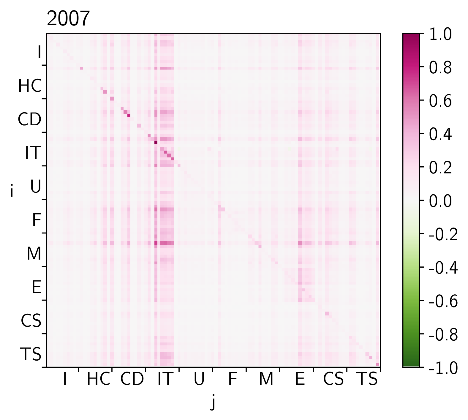
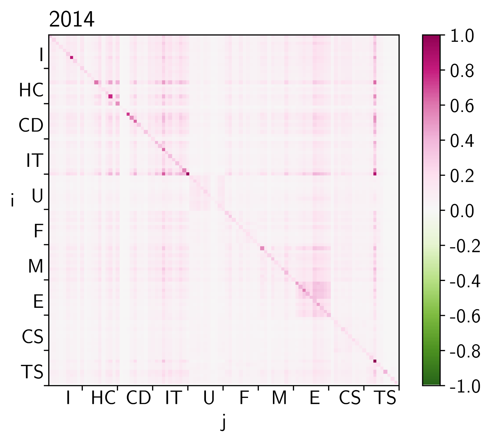
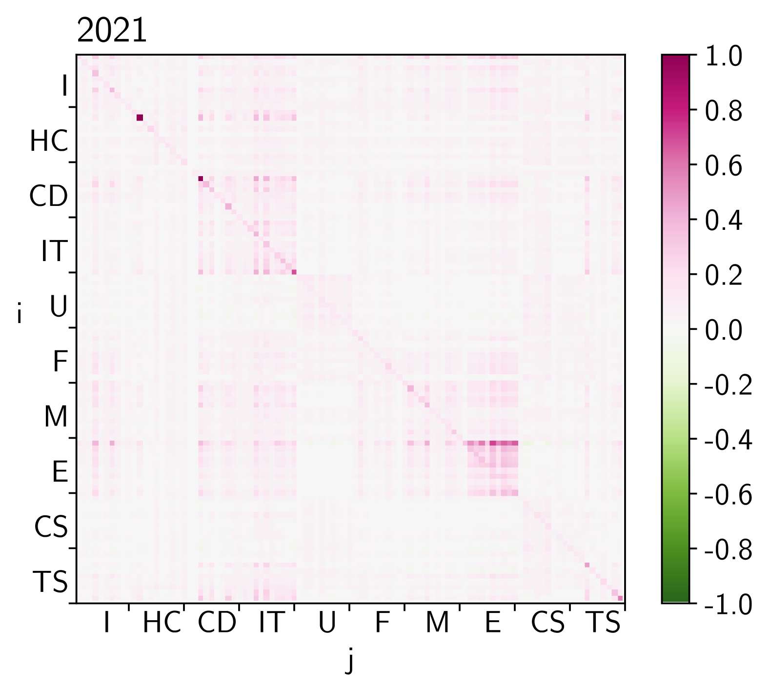
Figure 6: Matrices for the normalized responses including $\varepsilon_{i}(t)=0$ with entries $\rho_{ij}(\tau)$ for $i,j=1,\ldots,99$ at the time lag $\tau=30$ s in 2007, 2008, 2014 and 2021. The stocks pairs $(i,j)$ correspond to the sectors industrials (I), health care (HC), consumer discretionary (CD), information technology (IT), utilities (U), financials (F), materials (M), energy (E), consumer staples (CS), and telecommunications services (TS).

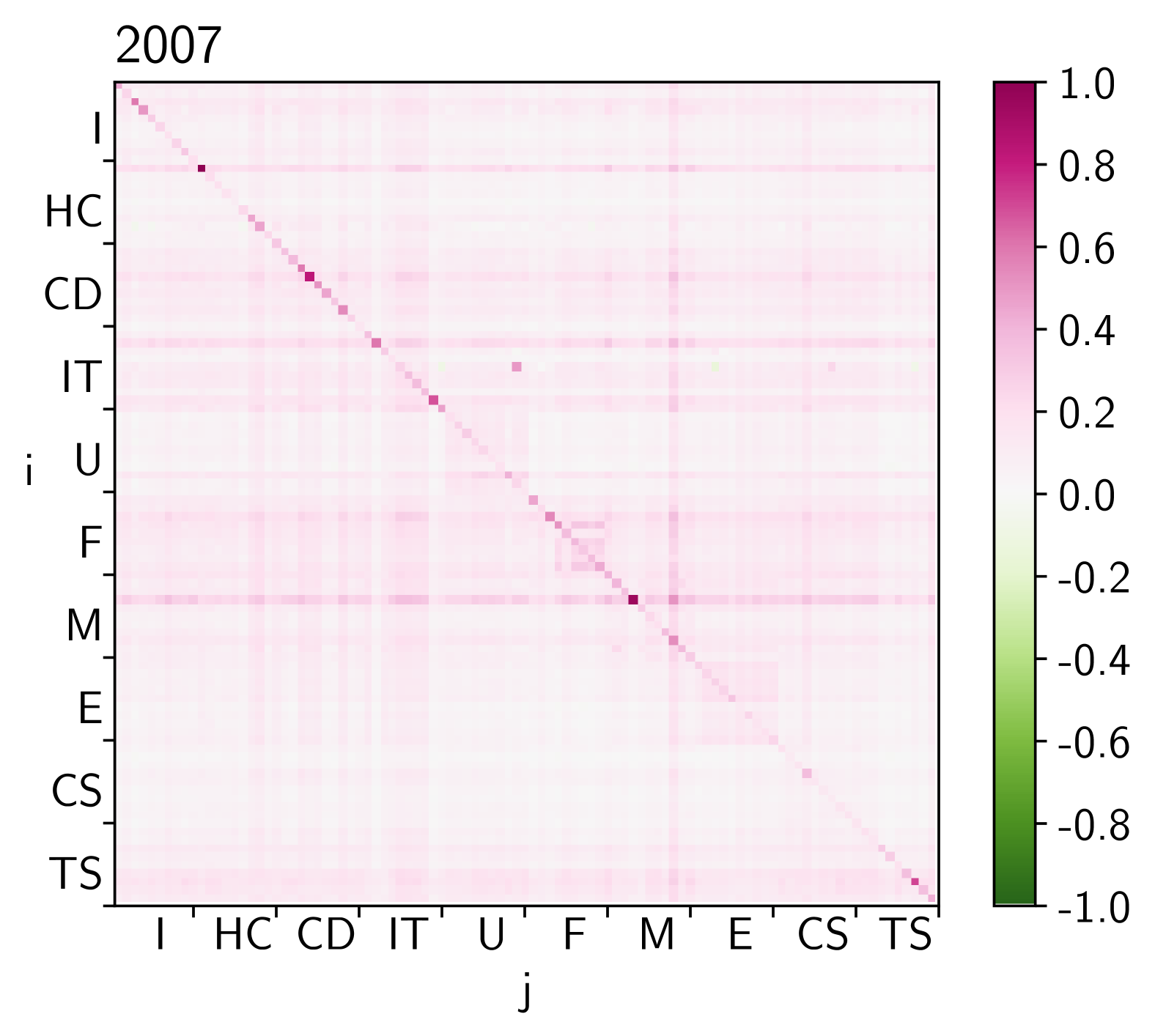
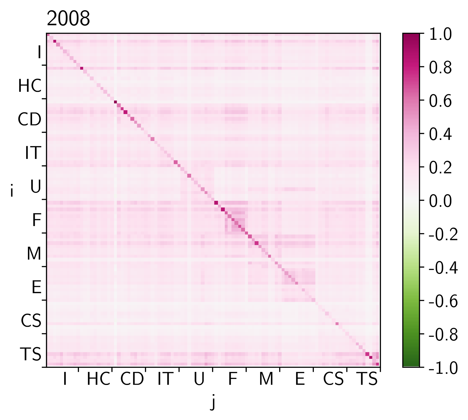
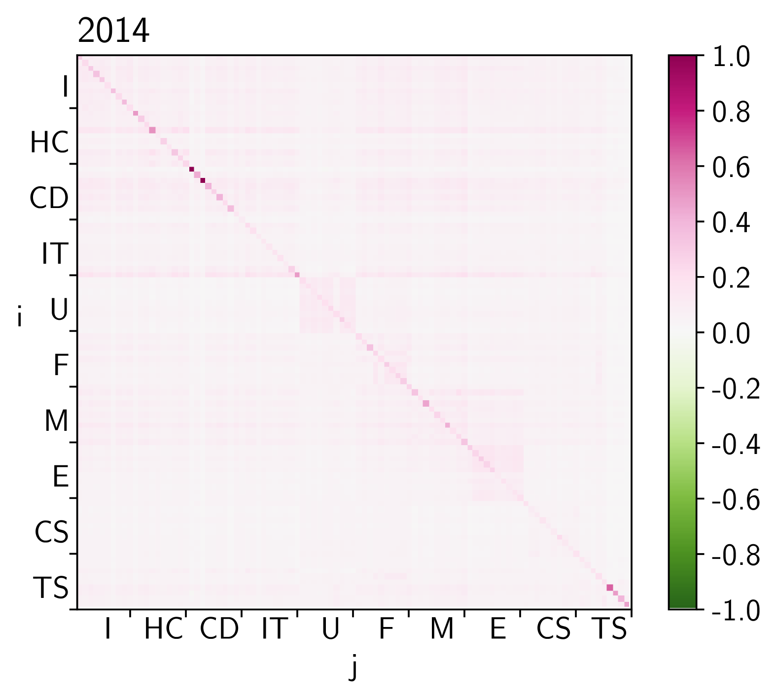
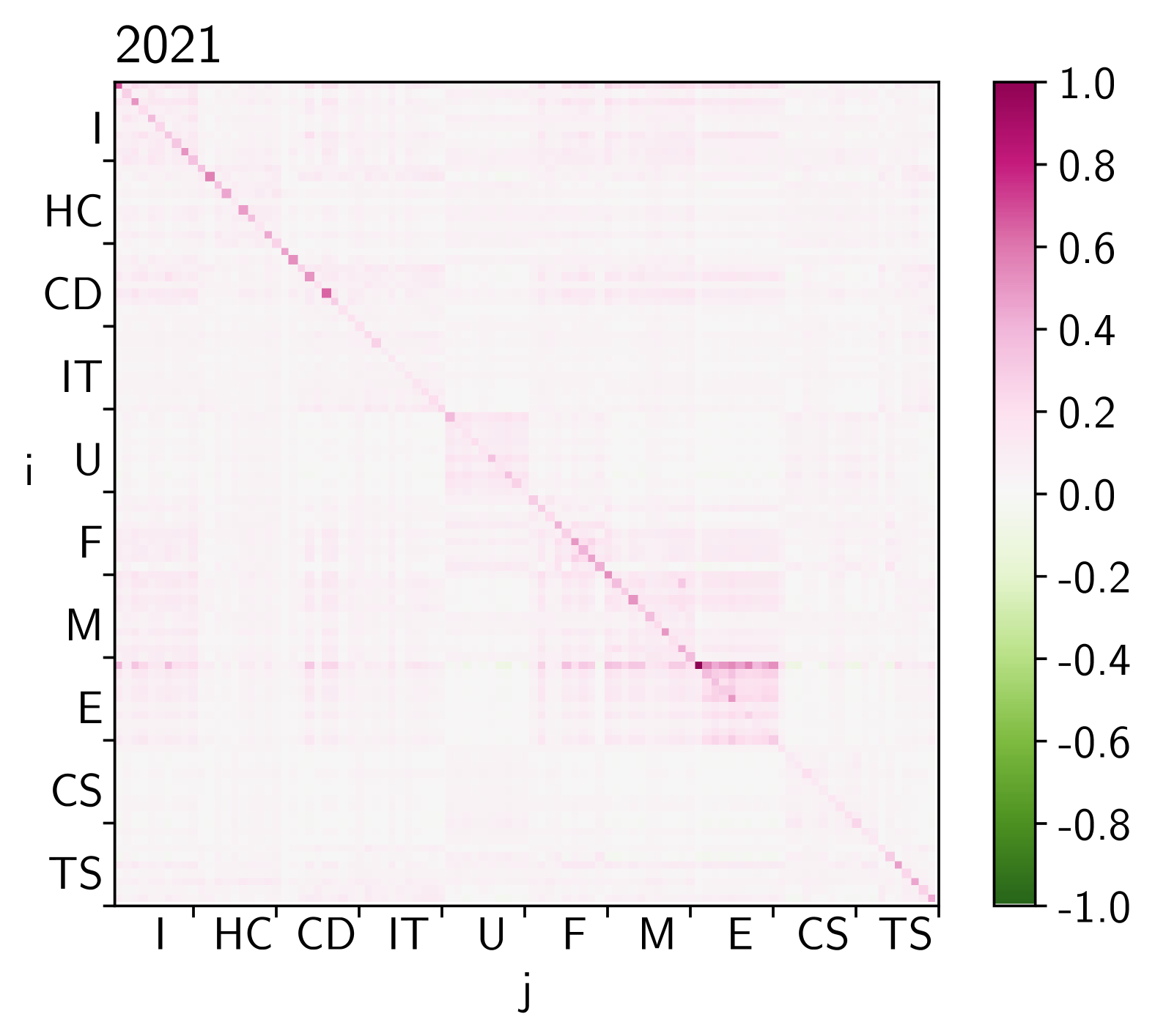
Figure 7: Matrices for the normalized responses excluding $\varepsilon_{i}(t)=0$ with entries $\rho_{ij}(\tau)$ for $i,j=1,\ldots,99$ at the time lag $\tau=30$ s in 2007, 2008, 2014 and 2021. The stocks pairs $(i,j)$ correspond to the sectors industrials (I), health care (HC), consumer discretionary (CD), information technology (IT), utilities (U), financials (F), materials (M), energy (E), consumer staples (CS), and telecommunications services (TS).

For all four years and a time lag of $\tau=30\,$s, the corresponding matrices in Figs. 6 and 7 show two kinds of gross patterns. First, as known from (symmetric) Pearson correlation matrices in financial markets [32, 33, 34], there are blocks along the main diagonal corresponding to industrial sectors which are uncovered after sorting those matrices according to the ten industrial sectors, see Sec. 2. Second, there are vertical and horizontal stripes that sometimes extend across all industrial sectors. For 2008, when we exclude $\varepsilon_{j}(t)=0$, the financial sector (F) has a more prominent block structure, while in 2021 the Energy sector (E) shows stronger responses when we include and exclude $\varepsilon_{j}(t)=0$. The vertical stripes emerge in 2007, 2008 and 2014 and almost not noticeable in 2021 when we include $\varepsilon_{i}(t)=0$. Excluding the case $\varepsilon_{i}(t)=0$, those stripes are replaced by broader, horizontal stripes in 2008.

4.5 Active and Passive Responses

To examine the structures of the market cross–responses more closely, we average for a fixed $i$ over all (pairwise) cross–responses

$$R_{i}^{(p)}(\tau)=\left\langle R_{ij}(\tau)\right\rangle_{j}\;,\quad\text{with $j\neq i$}$$ (18)

and for a fixed $j$ over all (pairwise) cross–responses

$$R_{j}^{(a)}(\tau)=\left\langle R_{ij}(\tau)\right\rangle_{i}\;,\quad\text{with $i\neq j$}\,.$$ (19)

The former is referred to as passive response function, the latter as active response function [18, 20]. The passive response function $R_{i}^{(p)}(\tau)$ quantifies the influence of all trade signs in the market on the return of stock $i$ with time lag $\tau$, the active response function $R_{j}^{(a)}(\tau)$ measures the influence of a trade or trades in stock $j$ on the returns of all other stocks with time lag $\tau$. In other words, index $i$ in $R_{i}^{(p)}(\tau)$ labels an influenced or impacted stock and index $j$ in $R_{j}^{(a)}(\tau)$ labels an influencing or impacting stock. Of course, every stock is influenced and is influencing at the same time.

Remarkably, Figs. 8 and 9 show a qualitative different behavior for active and passive responses.

\begin{overpic}[width=433.62pt]{Images/passive_response_function_2007_AAPL_GS_XOM.pdf} \put(61.0,22.0){\noindent\framebox{\parbox{22.76228pt}{2007}}} \end{overpic}

(a)

\begin{overpic}[width=433.62pt]{Images/active_response_function_2007_AAPL_GS_XOM.pdf} \put(71.0,22.0){\noindent\framebox{\parbox{22.76228pt}{2007}}} \end{overpic}

(b)

\begin{overpic}[width=433.62pt]{Images/passive_response_function_2008_AAPL_GS_XOM.pdf} \put(25.0,25.0){\noindent\framebox{\parbox{22.76228pt}{2008}}} \end{overpic}

(c)

\begin{overpic}[width=433.62pt]{Images/active_response_function_2008_AAPL_GS_XOM.pdf} \put(25.0,25.0){\noindent\framebox{\parbox{22.76228pt}{2008}}} \end{overpic}

(d)

Figure 8: Passive and active cross-response functions $R_{i}^{(p)}(\tau)$ and $R_{j}^{(a)}(\tau)$ for $i,j=\textrm{AAPL},\textrm{GS},\textrm{XOM}$ in the years 2007 and 2008 versus time lag $\tau$. Negative values for passive and active cross–responses are removed.

\begin{overpic}[width=433.62pt]{Images/passive_response_function_2014_AAPL_GS_XOM.pdf} \put(70.0,25.0){\noindent\framebox{\parbox{22.76228pt}{2014}}} \end{overpic}

(a)

\begin{overpic}[width=433.62pt]{Images/active_response_function_2014_AAPL_GS_XOM.pdf} \put(70.0,25.0){\noindent\framebox{\parbox{22.76228pt}{2014}}} \end{overpic}

(b)

\begin{overpic}[width=433.62pt]{Images/passive_response_function_2021_AAPL_GS_XOM.pdf} \put(25.0,25.0){\noindent\framebox{\parbox{22.76228pt}{2021}}} \end{overpic}

(c)

\begin{overpic}[width=433.62pt]{Images/active_response_function_2021_AAPL_GS_XOM.pdf} \put(25.0,25.0){\noindent\framebox{\parbox{22.76228pt}{2021}}} \end{overpic}

(d)

Figure 9: Passive and active cross-response functions $R_{i}^{(p)}(\tau)$ and $R_{j}^{(a)}(\tau)$ for $i,j=\textrm{AAPL},\textrm{GS},\textrm{XOM}$ in the years 2014 and 2021 versus time lag $\tau$. Negative values for passive and active cross–responses are removed.

In Refs. [16, 18], all stocks of the S&P 500 index in the respective year were averaged. Here, we exclusively use the stocks sorted according to the GICS, see Sec. 2. The results are qualitatively similar. In 2007 and 2008, the passive responses for AAPL and XOM begin to decrease after a much smaller time lag of length between $1000$ and $10000$ seconds. For 2014 and 2021, there is no separation of two different time scales between passive and active response. As seen for the market self– and cross–responses in Sec. 4.1, neither shows a systemic downward trend except for the active cross–response in 2021 for AAPL. The passive and active responses including $\varepsilon_{i}(t)=0$ are always smaller than those excluding $\varepsilon_{i}(t)=0$.

5 Conclusions

We considerably extended the studies of Refs. [16, 17, 18] to investigate the non–stationarity of non–Markovian effects. We found in the dynamics of the trading sizeable changes in the dynamics which reveals severe modifications in the traders’ actions. The market self– and cross–responses and the market trade sign self– and cross–correlators facilitate, at least their averaged versions, rather general observations and statements. How do the different results fit together? To what extent is the crisis year 2008 special?

There are two trends to be recognized over the years. First, the responses for the crisis year of 2008 are larger than for the other years. The self–responses for 2014 and 2021 remain on a higher level compared to 2007. Second, both market self–responses and cross–responses are strikingly less concave. The self–responses of 2014 and 2021 indicate that self–responses increasing for larger time lags are quite stable over time. Larger response values in times of crises and responses increasing for larger time lags may have different causes.

Around and during the financial crisis of 2008/2009 [35, 36, 37], algorithmic trading also increased dramatically [38]. Over the time period covered by our study, algorithmic trading has almost completely replaced traditional trading. Thus, trading may have been affected by both phenomena, the financial crisis itself as well as the surge in algorithmic trading. It is important to note that algorithmic trading does not only include high–frequency trades on very short time scales.

The increase in the response function may be related to the traders’ reaction to the financial crisis itself, as it increases from 2007 to 2008 within a relatively short period of time. In the liquidity game, liquidity providers are more alert placing their orders at more expensive price levels for the liquidity takers, i.e. liquidity providers demand a larger risk premium for compensation. The higher values in the self–responses for 2014 and 2021 compared to 2007 indicate that the crisis has had a lasting influence on the trader’s actions. Nevertheless, the cross–responses drop back to magnitudes similar to 2007. The shape of the self– and cross–responses is no longer concave for 2014 and 2021 hinting at different causes, i.e. the algorithmic trading might have changed the responses. One of the most notable changes in the traders’ behavior around 2008 is the change in passive and active cross–responses and might also be related to the change in algorithmic trading. The time scales of the passive and active response functions are different for 2007 and 2008, while we do not observe such behavior for 2014 and 2021.

Another interpretation is also possible if we assume that the change in response functions and the emergence of algorithmic trading coincide by chance. We know that the market operates in a new mode in terms of self–responses increasing for larger time lags. Even in a trading environment with exclusively human or algorithmic traders the market could have made a transition into a new stable state of trading due to a crisis that destabilized the subtle balance of the traders’ decisions.

The market trade sign correlators provide an indication of a major change from 2007 to 2008, moving towards a shorter memory between different stocks. A shorter memory in the liquidity game means that liquidity takers try to carry out their trading strategies more quickly. For 2014, the memory for the trade sign correlators becomes more similar to those of 2007. For 2021, the memory decreases again which might be explained by faster algorithmic trading. It is worth noting that the trade sign self–correlators are clearly different in 2021, with a second regime emerging. This regime is less noticeable for the other years. The second regime hints at a longer memory in the traders’ actions for larger time lags which might be related to a different traders’ strategy. The diffusive behavior of the returns resulting from a balance between sub– and superdiffusive dynamics behavior strongly depends on the time lag $\tau$.

In short, trading changed its phenomenology. The reasons cannot be fully disentangled, but important factors for the change in the traders’ interactions may be increased risk aversion due to the financial crisis of 2008/2009 and the rise of algorithmic trading. Our results indicate that the market mechanisms as borne out in the details of the order book are remarkably non–stationary. While the rules of the game do not change, it is now played in a different way. Close monitoring and careful data analysis over the years to come seems called for.

Appendix A Industrial Sectors and Stocks

Table 3: 99 stocks from ten economic sectors for 2008.

Industrials (I)			Financials (F)
Symbol	Company		Symbol	Company
FLR	Fluor Corp. (New)		CME	CME Group Inc.
LMT	Lockheed Martin Corp.		GS	Goldman Sachs Group
FLS	Flowserve Corporation		ICE	Intercontinental Exchange Inc.
PCP	Precision Castparts		AVB	AvalonBay Communities
LLL	L-3 Communications Holdings		BEN	Franklin Resources
UNP	Union Pacific		BXP	Boston Properties
BNI	Burlington Northern Santa Fe C		SPG	Simon Property Group Inc
FDX	FedEx Corporation		VNO	Vornado Realty Trust
GWW	Grainger (W.W.) Inc.		PSA	Public Storage
GD	General Dynamics		MTB	M$\&$T Bank Corp.
Health Care (HC)			Materials (M)
Symbol	Company		Symbol	Company
ISRG	Intuitive Surgical Inc.		X	United States Steel Corp.
BCR	Bard (C.R.) Inc.		MON	Monsanto Co.
BDX	Becton Dickinson		CF	CF Industries Holdings Inc
GENZ	Genzyme Corp.		FCX	Freeport-McMoran Cp $\&$ Gld
JNJ	Johnson $\&$ Johnson		APD	Air Products $\&$ Chemicals
LH	Laboratory Corp. of America Holding		PX	Praxair Inc.
ESRX	Express Scripts		VMC	Vulcan Materials
CELG	Celgene Corp.		ROH	Rohm $\&$ Haas
ZMH	Zimmer Holdings		NUE	Nucor Corp.
AMGN	Amgen		PPG	PPG Industries
Consumer Discretionary (CD)			Energy (E)
Symbol	Company		Symbol	Company
WPO	Washington Post		RIG	Transocean Inc. (New)
AZO	AutoZone Inc.		APA	Apache Corp.
SHLD	Sears Holdings Corporation		EOG	EOG Resources
WYNN	Wynn Resorts Ltd.		DVN	Devon Energy Corp.
AMZN	Amazon Corp.		HES	Hess Corporation
WHR	Whirlpool Corp.		XOM	Exxon Mobil Corp.
VFC	V.F. Corp.		SLB	Schlumberger Ltd.
APOL	Apollo Group		CVX	Chevron Corp.
NKE	NIKE Inc.		COP	ConocoPhillips
MCD	McDonald’s Corp.		OXY	Occidental Petroleum
Information Technology (IT)			Consumer Staples (CS)
Symbol	Company		Symbol	Company
GOOG	Google Inc.		BUD	Anheuser-Busch
MA	Mastercard Inc.		PG	Procter $\&$ Gamble
AAPL	Apple Inc.		CL	Colgate-Palmolive
IBM	International Bus. Machines		COST	Costco Co.
MSFT	Microsoft Corp.		WMT	Wal-Mart Stores
CSCO	Cisco Systems		PEP	PepsiCo Inc.
INTC	Intel Corp.		LO	Lorillard Inc.
QCOM	QUALCOMM Inc.		UST	UST Inc.
CRM	Salesforce Com Inc.		GIS	General Mills
WFR	MEMC Electronic Materials		KMB	Kimberly-Clark
Utilities (U)			Telecommunications Services (TS)
Symbol	Company		Symbol	Company
ETR	Entergy Corp.		T	AT$\&$T Inc.
EXC	Exelon Corp.		VZ	Verizon Communications
CEG	Constellation Energy Group		EQ	Embarq Corporation
FE	FirstEnergy Corp.		AMT	American Tower Corp.
FPL	FPL Group		CTL	Century Telephone
SRE	Sempra Energy		S	Sprint Nextel Corp.
STR	Questar Corp.		Q	Qwest Communications Int
TEG	Integrys Energy Group Inc.		WIN	Windstream Corporation
EIX	Edison Int’l		FTR	Frontier Communications
AYE	Allegheny Energy

Table 4: 99 stocks from ten economic sectors for 2007. Stocks in bold represent new stocks compared to 2008.

Industrials (I)			Financials (F)
Symbol	Company		Symbol	Company
FLR	Fluor Corp. (New)		CME	CME Group Inc.
LMT	Lockheed Martin Corp.		GS	Goldman Sachs Group
FLS	Flowserve Corporation		ICE	Intercontinental Exchange Inc.
PCP	Precision Castparts		AVB	AvalonBay Communities
LLL	L-3 Communications Holdings		BEN	Franklin Resources
UNP	Union Pacific		BXP	Boston Properties
MMM	3M Company		SPG	Simon Property Group Inc
FDX	FedEx Corporation		VNO	Vornado Realty Trust
GWW	Grainger (W.W.) Inc.		PSA	Public Storage
GD	General Dynamics		MTB	M$\&$T Bank Corp.
Health Care (HC)			Materials (M)
Symbol	Company		Symbol	Company
ISRG	Intuitive Surgical Inc.		X	United States Steel Corp.
BCR	Bard (C.R.) Inc.		MON	Monsanto Co.
BDX	Becton Dickinson		CF	CF Industries Holdings Inc
ABT	Abbott Laboratories		FCX	Freeport-McMoran Cp $\&$ Gld
JNJ	Johnson $\&$ Johnson		APD	Air Products $\&$ Chemicals
LH	Laboratory Corp. of America Holding		PX	Praxair Inc.
ESRX	Express Scripts		VMC	Vulcan Materials
CELG	Celgene Corp.		SIAL	Sigma Aldrich Corp.
ZMH	Zimmer Holdings		NUE	Nucor Corp.
AMGN	Amgen		PPG	PPG Industries
			SHW	Sherwin–Williams Company
Consumer Discretionary (CD)			Energy (E)
Symbol	Company		Symbol	Company
AZO	AutoZone Inc.		NBL	Noble Energy Inc.
SHLD	Sears Holdings Corporation		APA	Apache Corp.
WYNN	Wynn Resorts Ltd.		EOG	EOG Resources
AMZN	Amazon Corp.		DVN	Devon Energy Corp.
WHR	Whirlpool Corp.		HES	Hess Corporation
VFC	V.F. Corp.		XOM	Exxon Mobil Corp.
APOL	Apollo Group		SLB	Schlumberger Ltd.
NKE	NIKE Inc.		CVX	Chevron Corp.
MCD	McDonald’s Corp.		COP	ConocoPhillips
			OXY	Occidental Petroleum
Information Technology (IT)			Consumer Staples (CS)
Symbol	Company		Symbol	Company
GOOG	Google Inc.		CLX	The Colrox Company
MA	Mastercard Inc.		PG	Procter $\&$ Gamble
AAPL	Apple Inc.		CL	Colgate-Palmolive
IBM	International Bus. Machines		COST	Costco Co.
MSFT	Microsoft Corp.		WMT	Wal-Mart Stores
CSCO	Cisco Systems		PEP	PepsiCo Inc.
INTC	Intel Corp.		KO	The Coca-Cola Company
QCOM	QUALCOMM Inc.		K	Kellogg Company
CRM	Salesforce Com Inc.		GIS	General Mills
WFR	MEMC Electronic Materials		KMB	Kimberly-Clark
Utilities (U)			Telecommunications Services (TS)
Symbol	Company		Symbol	Company
ETR	Entergy Corp.		T	AT$\&$T Inc.
EXC	Exelon Corp.		VZ	Verizon Communications
CEG	Constellation Energy Group		DTV	DirecTV Group Inc.
FE	FirstEnergy Corp.		AMT	American Tower Corp.
PCG	PG$\&E$ Corp		CTL	Century Telephone
SRE	Sempra Energy		S	Sprint Nextel Corp.
D	Dominion Energy Inc.		TLAB	Tellabs Inc.
TEG	Integrys Energy Group Inc.		WIN	Windstream Corporation
EIX	Edison Int’l		CMCSA	Comcast Corp.
SO	The Southern Company

Table 5: 99 stocks from ten economic sectors for 2014. Stocks in bold represent new stocks compared to 2008.

Industrials (I)			Financials (F)
Symbol	Company		Symbol	Company
FLR	Fluor Corp. (New)		CME	CME Group Inc.
LMT	Lockheed Martin Corp.		GS	Goldman Sachs Group
FLS	Flowserve Corporation		ICE	Intercontinental Exchange Inc.
PCP	Precision Castparts		AVB	AvalonBay Communities
LLL	L-3 Communications Holdings		BEN	Franklin Resources
UNP	Union Pacific		BXP	Boston Properties
AAL	American Airlines Group Inc.		SPG	Simon Property Group Inc
FDX	FedEx Corporation		VNO	Vornado Realty Trust
GWW	Grainger (W.W.) Inc.		PSA	Public Storage
GD	General Dynamics		MTB	M$\&$T Bank Corp.
Health Care (HC)			Materials (M)
Symbol	Company		Symbol	Company
ISRG	Intuitive Surgical Inc.		X	United States Steel Corp.
BCR	Bard (C.R.) Inc.		MON	Monsanto Co.
BDX	Becton Dickinson		CF	CF Industries Holdings Inc
BIIB	Biogen Idec Inc..		FCX	Freeport-McMoran Cp $\&$ Gld
JNJ	Johnson $\&$ Johnson		APD	Air Products $\&$ Chemicals
LH	Laboratory Corp. of America Holding		PX	Praxair Inc.
ESRX	Express Scripts		VMC	Vulcan Materials
CELG	Celgene Corp.		DOW	DOW Chemicals Co. Com.
ZMH	Zimmer Holdings		NUE	Nucor Corp.
AMGN	Amgen		PPG	PPG Industries
Consumer Discretionary (CD)			Energy (E)
Symbol	Company		Symbol	Company
GHC	Graham Holdings		RIG	Transocean Inc. (New)
AZO	AutoZone Inc.		APA	Apache Corp.
SHLD	Sears Holdings Corporation		EOG	EOG Resources
WYNN	Wynn Resorts Ltd.		DVN	Devon Energy Corp.
AMZN	Amazon Corp.		HES	Hess Corporation
WHR	Whirlpool Corp.		XOM	Exxon Mobil Corp.
VFC	V.F. Corp.		SLB	Schlumberger Ltd.
APOL	Apollo Group		CVX	Chevron Corp.
NKE	NIKE Inc.		COP	ConocoPhillips
MCD	McDonald’s Corp.		OXY	Occidental Petroleum
Information Technology (IT)			Consumer Staples (CS)
Symbol	Company		Symbol	Company
GOOG	Google Inc.		BUD	Anheuser-Busch
MA	Mastercard Inc.		PG	Procter $\&$ Gamble
AAPL	Apple Inc.		CL	Colgate-Palmolive
IBM	International Bus. Machines		COST	Costco Co.
MSFT	Microsoft Corp.		WMT	Wal-Mart Stores
CSCO	Cisco Systems		PEP	PepsiCo Inc.
INTC	Intel Corp.		LO	Lorillard Inc.
QCOM	QUALCOMM Inc.		MO	Altria Group Inc.
CRM	Salesforce Com Inc.		GIS	General Mills
SUNE	Sunedison Inc. Com.		KMB	Kimberly-Clark
Utilities (U)			Telecommunications Services (TS)
Symbol	Company		Symbol	Company
ETR	Entergy Corp.		T	AT$\&$T Inc.
EXC	Exelon Corp.		VZ	Verizon Communications
DUK	Duke Energy Corp. Com.		FB	Facebook Inc. Com.
FE	FirstEnergy Corp.		AMT	American Tower Corp.
NEE	NextEra Energy Inc. Com.		CTL	Century Telephone
SRE	Sempra Energy		S	Sprint Nextel Corp.
STR	Questar Corp.		Q	Qwest Communications Int
TEG	Integrys Energy Group Inc.		WIN	Windstream Corporation
EIX	Edison Int’l		FTR	Frontier Communications
SO	Southern Com.

Table 6: 99 stocks from ten economic sectors for 2021. Stocks in bold represent new stocks compared to 2014. Stocks in italicized represent new stocks compared to 2008.

Industrials (I)			Financials (F)
Symbol	Company		Symbol	Company
FLR	Fluor Corp. (New)		CME	CME Group Inc.
LMT	Lockheed Martin Corp.		GS	Goldman Sachs Group
FLS	Flowserve Corporation		ICE	Intercontinental Exchange Inc.
BA	The Boeing Company		AVB	AvalonBay Communities
LHX	L3 Harris Technologies		BEN	Franklin Resources
UNP	Union Pacific		BXP	Boston Properties
AAL	American Airlines Group Inc.		SPG	Simon Property Group Inc
FDX	FedEx Corporation		VNO	Vornado Realty Trust
GWW	Grainger (W.W.) Inc.		PSA	Public Storage
GD	General Dynamics		MTB	M$\&$T Bank Corp.
Health Care (HC)			Materials (M)
Symbol	Company		Symbol	Company
ISRG	Intuitive Surgical Inc.		X	United States Steel Corp.
MRNA	Moderna Inc.		VALE	Vale S.A.
BDX	Becton Dickinson		CF	CF Industries Holdings Inc
BIIB	Biogen Idec Inc..		FCX	Freeport-McMoran Cp $\&$ Gld
JNJ	Johnson $\&$ Johnson		APD	Air Products $\&$ Chemicals
LH	Laboratory Corp. of America Holding		LIN	Linde plc.
CI	Cigna Corp		VMC	Vulcan Materials
BMY	Bristol-Meyers Squibb		DOW	DOW Chemicals Co. Com.
ZBH	Zimmer Biomet Holdings Inc.		NUE	Nucor Corp.
AMGN	Amgen		PPG	PPG Industries
Consumer Discretionary (CD)			Energy (E)
Symbol	Company		Symbol	Company
GHC	Graham Holdings		RIG	Transocean Inc. (New)
AZO	AutoZone Inc.		APA	Apache Corp.
TSLA	Tesla Inc		EOG	EOG Resources
WYNN	Wynn Resorts Ltd.		DVN	Devon Energy Corp.
AMZN	Amazon Corp.		HES	Hess Corporation
WHR	Whirlpool Corp.		XOM	Exxon Mobil Corp.
VFC	V.F. Corp.		SLB	Schlumberger Ltd.
BABA	Alibaba		CVX	Chevron Corp.
NKE	NIKE Inc.		COP	ConocoPhillips
MCD	McDonald’s Corp.		OXY	Occidental Petroleum
Information Technology (IT)			Consumer Staples (CS)
Symbol	Company		Symbol	Company
GOOG	Google Inc.		BUD	Anheuser-Busch
MA	Mastercard Inc.		PG	Procter $\&$ Gamble
AAPL	Apple Inc.		CL	Colgate-Palmolive
IBM	International Bus. Machines		COST	Costco Co.
MSFT	Microsoft Corp.		WMT	Wal-Mart Stores
CSCO	Cisco Systems		PEP	PepsiCo Inc.
INTC	Intel Corp.		BTI	British American Tobacco
QCOM	QUALCOMM Inc.		MO	Altria Group Inc.
CRM	Salesforce Com Inc.		GIS	General Mills
NVDA	Nvidia Corp.		KMB	Kimberly-Clark
Utilities (U)			Telecommunications Services (TS)
Symbol	Company		Symbol	Company
ETR	Entergy Corp.		T	AT$\&$T Inc.
EXC	Exelon Corp.		VZ	Verizon Communications
DUK	Duke Energy Corp. Com.		FB	Facebook Inc. Com.
FE	FirstEnergy Corp.		AMT	American Tower Corp.
NEE	NextEra Energy Inc. Com.		LUMN	Lumen Technologies
SRE	Sempra Energy		TMUS	T-Mobile US Inc.
D	Dominion Energy Inc.		IQV	IQVIA Holdings Inc.
WEC	WEC Energy Group		NFLX	Netflix Inc.
EIX	Edison Int’l		BIDU	Baidu Inc.
SO	Southern Com.

References

- [1] J.-P. Bouchaud, J. D. Farmer, F. Lillo, CHAPTER 2 - How Markets Slowly Digest Changes in Supply and Demand, in: T. Hens, K. R. Schenk-Hoppé (Eds.), Handbook of Financial Markets: Dynamics and Evolution, Handbooks in Finance, North-Holland, San Diego, 2009, pp. 57–160. doi:https://doi.org/10.1016/B978-012374258-2.50006-3.
- [2] J.-P. Bouchaud, Price Impact: Information Revelation or Self-Fulfilling Prophecies?, Cambridge University Press, 2023, p. 101–106. doi:https://doi.org/10.1016/B978-012374258-2.50006-3.
- [3] F. Lillo, Order flow and price formation, Cambridge University Press, 2023, p. 107–129. doi:https://doi.org/10.1016/B978-012374258-2.50006-3.
- [4] D. M. Cutler, J. M. Poterba, L. H. Summers, What Moves Stock Prices?, Princeton University Press, Princeton, 1989, pp. 56–64. doi:https://doi.org/10.1515/9781400829408-008.
- [5] R. Fair, Events That Shook the Market, The Journal of Business 75 (4) (2002) 713–731, full publication date: October 2002. doi:https://doi.org/10.1086/341640.
- [6] A. Joulin, A. Lefevre, D. Grunberg, J. P. Bouchaud, Stock price jumps: news and volume play a minor role, Wilmott Magazine (2008) 1–7.
- [7] J. Hasbrouk, Measuring the information content of stock trades, The Journal of Finance 46 (1) (1991) 179–207. doi:https://doi.org/10.1111/j.1540-6261.1991.tb03749.x.
-
[8]
J.-P. Bouchaud, Y. Gefen, M. Potters, M. Wyart,
Fluctuations and
response in financial markets: the subtle nature of ‘random’ price changes,
Quantitative Finance 4 (2) (2003) 176.
doi:10.1088/1469-7688/4/2/007.
URL https://dx.doi.org/10.1088/1469-7688/4/2/007 - [9] F. Lillo, J. D. Farmer, The Long Memory of the Efficient Market, Studies in Nonlinear Dynamics & Econometrics 8 (3) (2004) 20123001. doi:https://doi.org/doi:10.2202/1558-3708.1226.
- [10] F. Lillo, S. Mike, J. D. Farmer, Theory for long memory in supply and demand, Phys. Rev. E 71 (2005) 066122. doi:https://doi.org/10.1103/PhysRevE.71.066122.
- [11] A. Gerig, A theory for market impact: How order flow affects stock price (2008). arXiv:0804.3818.
-
[12]
B. Tóth, I. Palit, F. Lillo, J. D. Farmer,
Why
is equity order flow so persistent?, Journal of Economic Dynamics and
Control 51 (2015) 218–239.
doi:https://doi.org/10.1016/j.jedc.2014.10.007.
URL https://www.sciencedirect.com/science/article/pii/S0165188914002826 -
[13]
J.-P. Bouchaud,
Chapter
7 - agent-based models for market impact and volatility, in: C. Hommes,
B. LeBaron (Eds.), Handbook of Computational Economics, Vol. 4 of Handbook of
Computational Economics, Elsevier, 2018, pp. 393–436.
doi:https://doi.org/10.1016/bs.hescom.2018.02.002.
URL https://www.sciencedirect.com/science/article/pii/S1574002118300029 - [14] J.-P. Bouchaud, J. Kockelkoren, M. Potters, Random walks, liquidity molasses and critical response in financial markets, Quantitative Finance 6 (2) (2006) 115–123. doi:10.1080/14697680500397623.
- [15] E. F. Fama, Efficient capital markets: A review of theory and empirical work*, The Journal of Finance 25 (2) (1970) 383–417.
- [16] S. Wang, R. Schäfer, T. Guhr, Price response in correlated financial markets: empirical results, arXiv:1510.03205 (2016).
- [17] S. Wang, R. Schäfer, T. Guhr, Cross-response in correlated financial markets: individual stocks, The European Physical Journal B 89 (4) (2016) 105, arXiv:1603.01580. doi:https://doi.org/10.1140/epjb/e2016-60818-y.
- [18] S. Wang, R. Schäfer, T. Guhr, Average cross-responses in correlated financial markets, The European Physical Journal B 89 (9) (2016) 207, arXiv:1603.01586. doi:https://doi.org/10.1140/epjb/e2016-70137-0.
-
[19]
M. Benzaquen, I. Mastromatteo, Z. Eisler, J.-P. Bouchaud,
Dissecting cross-impact on
stock markets: an empirical analysis, Journal of Statistical Mechanics:
Theory and Experiment 2017 (2) (2017) 023406.
doi:10.1088/1742-5468/aa53f7.
URL https://dx.doi.org/10.1088/1742-5468/aa53f7 -
[20]
S. Wang, T. Guhr, Microscopic
understanding of cross-responses between stocks: A two-component price impact
model, Market Microstructure and Liquidity 03 (03n04) (2017) 1850009.
arXiv:https://doi.org/10.1142/S2382626618500090, doi:10.1142/S2382626618500090.
URL https://doi.org/10.1142/S2382626618500090 -
[21]
S. Grimm, T. Guhr, How spread
changes affect the order book: comparing the price responses of order
deletions and placements to trades, The European Physical Journal B 92 (6)
(2019) 133.
doi:10.1140/epjb/e2019-90744-3.
URL https://doi.org/10.1140/epjb/e2019-90744-3 - [22] J. C. Henao-Londono, S. M. Krause, T. Guhr, Price response functions and spread impact in correlated financial markets, The European Physical Journal B 94 (4) (2021) 78. doi:https://doi.org/10.1140/epjb/s10051-021-00077-z.
- [23] J. C. Henao-Londono, T. Guhr, Foreign exchange markets: Price response and spread impact, Physica A: Statistical Mechanics and its Applications 589 (2022) 126587. doi:https://doi.org/10.1016/j.physa.2021.126587.
-
[24]
J. Hasbrouck, D. J. Seppi,
Common
factors in prices, order flows, and liquidity, Journal of Financial
Economics 59 (3) (2001) 383–411.
doi:https://doi.org/10.1016/S0304-405X(00)00091-X.
URL https://www.sciencedirect.com/science/article/pii/S0304405X0000091X - [25] M. Schneider, F. Lillo, Cross-impact and no-dynamic-arbitrage, Quantitative Finance 19 (1) (2019) 137–154. arXiv:https://doi.org/10.1080/14697688.2018.1467033, doi:10.1080/14697688.2018.1467033.
- [26] R. Cont, M. Cucuringu, C. Zhang, Cross–impact of order flow imbalance in equity markets, Quantitative Finance 23 (10) (2023) 1373–1393. doi:10.1080/14697688.2023.2236159.
- [27] V. L. Coz, I. Mastromatteo, D. Challet, M. Benzaquen, When is cross impact relevant?, Quantitative Finance 24 (2) (2024) 265–279. doi:10.1080/14697688.2024.2302827.
- [28] F. Capponi, R. Cont, Multi-asset market impact and order flow commonality, Available at SSRN 3706390 (2020).
- [29] New York stock exchange, Daily TAQ (Trade and Quote), https://www.nyse.com/market-data/academics (2014).
-
[30]
S. M. Duarte Queirós,
Trading
volume in financial markets: An introductory review, Chaos, Solitons &
Fractals 88 (2016) 24–37, complexity in Quantitative Finance and Economics.
doi:https://doi.org/10.1016/j.chaos.2015.12.024.
URL https://www.sciencedirect.com/science/article/pii/S0960077916000023 - [31] J. Beran, Statistics for Long-Memory Processes, Chapman and Hall/CRC, Boca Raton, London, New York, Washington, D .C ., 1994.
-
[32]
L. Laloux, P. Cizeau, J.-P. Bouchaud, M. Potters,
Noise Dressing
of Financial Correlation Matrices, Phys. Rev. Lett. 83 (1999) 1467–1470.
doi:10.1103/PhysRevLett.83.1467.
URL https://link.aps.org/doi/10.1103/PhysRevLett.83.1467 -
[33]
V. Plerou, P. Gopikrishnan, B. Rosenow, L. A. N. Amaral, T. Guhr, H. E.
Stanley, Random
matrix approach to cross correlations in financial data, Phys. Rev. E 65
(2002) 066126.
doi:10.1103/PhysRevE.65.066126.
URL https://link.aps.org/doi/10.1103/PhysRevE.65.066126 -
[34]
T. Guhr, B. Kälber, A
new method to estimate the noise in financial correlation matrices, Journal
of Physics A: Mathematical and General 36 (12) (2003) 3009.
doi:10.1088/0305-4470/36/12/310.
URL https://dx.doi.org/10.1088/0305-4470/36/12/310 -
[35]
A. J. Heckens, S. M. Krause, T. Guhr,
Uncovering the dynamics
of correlation structures relative to the collective market motion, Journal
of Statistical Mechanics: Theory and Experiment 2020 (10) (2020) 103402.
doi:10.1088/1742-5468/abb6e2.
URL https://doi.org/10.1088%2F1742-5468%2Fabb6e2 -
[36]
A. J. Heckens, T. Guhr, A new
attempt to identify long-term precursors for endogenous financial crises in
the market correlation structures, Journal of Statistical Mechanics: Theory
and Experiment 2022 (4) (2022) 043401.
doi:10.1088/1742-5468/ac59ab.
URL https://doi.org/10.1088/1742-5468/ac59ab -
[37]
A. J. Heckens, T. Guhr,
New
collectivity measures for financial covariances and correlations, Physica A:
Statistical Mechanics and its Applications 604 (2022) 127704.
doi:https://doi.org/10.1016/j.physa.2022.127704.
URL https://www.sciencedirect.com/science/article/pii/S0378437122004666 - [38] R. Kissell, Algorithmic trading methods: Applications using advanced statistics, optimization, and machine learning techniques, Academic Press, London, San Diego, Cambridge, Oxford, 2020.