Boosting MCSat Modulo Nonlinear Integer Arithmetic via Local Search

Abstract

The Model Constructing Satisfiability (MCSat) approach to the SMT problem extends the ideas of CDCL from the SAT level to the theory level. Like SAT, its search is driven by incrementally constructing a model by assigning concrete values to theory variables and performing theory-level reasoning to learn lemmas when conflicts arise. Therefore, the selection of values can significantly impact the search process and the solver’s performance. In this work, we propose guiding the MCSat search by utilizing assignment values discovered through local search. First, we present a theory-agnostic framework to seamlessly integrate local search techniques within the MCSat framework. Then, we highlight how to use the framework to design a search procedure for (quantifier-free) Nonlinear Integer Arithmetic ($\mathcal{NIA}$), utilizing accelerated hill-climbing and a new operation called feasible-sets jumping. We implement the proposed approach in the MCSat engine of the Yices2 solver, and empirically evaluate its performance over the $\mathcal{NIA}$ benchmarks of SMT-LIB.

1 Introduction

smt is the problem of deciding the satisfiability of a first-order formula with respect to defined background theories. satisfiability modulo theory (SMT) solvers are the core backbone of a vast range of verification and synthesis tools that require reasoning about expressive logical theories such as real/integer arithmetic [3, 16]. One of the major state-of-the-art approaches to SMT is the Model Constructing Satisfiability calculus (MCSat) [28, 15], which generalizes the ideas of Conflict-Driven Clause Learning (CDCL) to the theory level, and which has been shown to perform particularly well on complex theories such as nonlinear arithmetic. In the MCSat approach, the solver progressively constructs a theory model, similarly to how SAT solvers construct Boolean models. Theory reasoning is used to assess the consistency of partial models, provide explanations of infeasibility, decide theory variables, and propagate theory constraints.

When extending the partial model with a new assignment to a theory variable, picking a good value is critical for the overall performance of the solver. Heuristics used by state-of-the-art solvers pick values on the basis of compatibility with the current search state and of computational cheapness. This has a major drawback: these heuristics only consider knowledge of the current search state, neglecting information on how likely a particular assignment is to lead to a satisfying model eventually.

In this work, we address the problem of choosing good values for variable decisions by augmenting the current search state knowledge with insights provided by local search techniques. Following the logic-to-optimization approach [19, 36], we associate to the logical formula a cost function that represents the distance from a model, and use local search to find assignments that have a small cost. These assignments are then used to guide future MCSat decisions.

Although local search has already been used in the context of SMT, either as a standalone solver [44, 34, 6] or as a CDCL(T) theory solver [46], our work is the first to propose a tight integration of local search within the MCSat framework, creating a powerful synergy between the reasoning capabilities of MCSat and the intuition provided by local search which boosts performance for both satisfiable and unsatisfiable instances. Our novel approach is flexible enough to allow calls to local search at any point during the MCSat search, seamlessly fitting with the current state. As MCSat progresses through decisions, propagations, and conflicts, the local search problem is instantiated accordingly: (i) the cost function is built upon the simplification of the original formula under current state assumptions, (ii) initial local search assignments are based on the current search state represented by the trail and on the value cache, and (iii) local search moves are enhanced by information on the feasibility sets.

While our approach can be applied to any theory supported by MCSat, in this work we showcase its application to the theory of nonlinear integer arithmetic ($\mathcal{NIA}$). In particular, we design a procedure based on a new operation called feasible-sets jumping, which allows to move between feasible intervals, and on accelerated hill-climbing [25], to move inside feasible intervals.

Contributions.

In this work we (i) design a theory-agnostic framework to tightly integrate local search techniques within the MCSat approach in order to guide variable decisions, (ii) use the framework to define a local search procedure for the theory of nonlinear integer arithmetic, that makes use of feasible-sets jumping and accelerated hill-climbing, and (iii) show the practical applicability of our method using our implementation in the MCSat engine of Yices2 [17] on the quantifier-free $\mathcal{NIA}$ benchmark set of SMT-LIB [2].

Structure.

In Section 2, we provide the necessary background. Section 3 describes a deep integration of local search techniques within the MCSat framework from a general point of view, which is applied in Section 4 to define a local search approach for non-linear integer arithmetic. In Section 5, we show and discuss the results of our experiments before presenting related work in Section 6 and concluding in Section 7.

2 Preliminaries

We assume basic knowledge on the standard first-order quantifier-free logical setting and standard notions of theory, satisfiability, and logical consequence. We write logical variables with $x,y,\ldots$, and concrete values with $\alpha,\beta,\ldots$ (the domain of concrete values is theory specific, e.g. $\mathbb{Z}$ for integer arithmetic, $\mathbb{R}$ for real arithmetic). An assignment $\mu$ is a map from variables to values of matching type. If $\phi$ is a formula, we denote with $\mathit{Vars}({\phi})$ the set of its (free) variables. We use $C$ to denote clauses, and $L$ to denote literals. We use $p,q$ to denote logic symbols representing polynomials. Nonlinear Integer Arithmetic ($\mathcal{NIA}$) is the theory consisting of arbitrary Boolean combinations of Boolean variables and arithmetic atoms of the form of polynomial equalities and polynomial inequalities over integer variables. It is undecidable by Matiyasevich’s theorem [38].

2.1 SMT & MCSat

SMT [3] is the problem of deciding the satisfiability of a first-order formula with respect to some theory or combination of theories. Two of the major approaches for SMT solving are the with theory support (CDCL(T)) [40, 3] and the MCSat approach. In the former, theory solvers augment a propositional SAT engine with theory reasoning procedures which are capable of deciding a conjunction of literals (i.e. atomic formulas and their negations) in a particular theory. A propositional model (of the Boolean abstraction of the formula) found by the SAT solver is then checked by all theory engines for theory consistency.

The latter, MCSat, applies CDCL-like mechanisms to perform theory reasoning directly. It can be used either as a theory solver for a specific theory (e.g. in Z3 [14] for non-linear arithmetic over the reals and the integers [4]), or as a fully-fledged stand-alone engine able to handle multiple theories (e.g. in Yices2 for non-linear arithmetic over the reals [29] and over the integers [27], bit-vectors [21], arrays [26], and finite fields [24, 23]; as well as in SMT-RAT [13] for non-linear real arithmetic [32]). The MCSat architecture consists of a core solver, an assignment trail, and plugins for theory reasoning. Figure 1 illustrates the high level flow of the MCSat framework.

The core solver incrementally constructs a partial model consisting of Boolean and theory assignments (stored in a trail), ensuring its consistency with the constraints. The trail contains three kinds of elements: propagated literals (literals implied to be true by the current state), decided literals (literals that we assume to be true), and model assignments (assignments of first-order variables to concrete values). Propagations, conflict analysis, lemmas generation, and variable decisions are all handled by theory plugins (including a Boolean plugin that is responsible for propositional reasoning). In general, plugins also keep a feasibility set for each variable of their competence, containing the values that are consistent with the current trail and are, thus, candidates to be picked for deciding the variable.

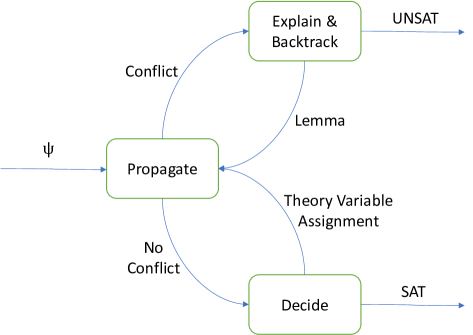
Figure 1: The MCSat framework consists of the following steps: 1) Propagate the trail. 2) If a conflict is found during propagation, check if there is any decision to backtrack over. If not, return UNSAT. Otherwise, explain the conflict using a lemma, backtrack the trail, and repeat step 1. 3) If no conflict is found during propagation, decide on a variable that is not on the trail. If there is nothing left to decide, return SAT. Otherwise, add the decided variable to the trail and repeat step 1.

When the core solver selects a variable for decision, the choice of the value to assign to the variable is competence of the theory plugin responsible for its type. Some solvers (e.g. Yices2) implements a heuristic called value caching (a generalization of SAT phase saving [41]), that keeps track of the last value assigned to a variable when the assignment is undone. Then, when a decision has to be made for the variable, the cached value will be used, provided that it is still in the feasible set (otherwise, it will simply be ignored).

In the following, we will denote with $M$ the trail, with $v[M](x)$ the value of the variable $x$ in the trail (which may be equal to $\mathtt{undef}$ if the variable is not assigned in the trail), and with $v[M](L)$ the truth value of the literal $L$ in the trail (which may be true ($\top$), false ($\bot$), or $\mathtt{undef}$). We denote with $\mathit{feasible}(x)$ the feasibility set of $x$, i.e. all values that can be chosen for $x$ in the current search state. For arithmetical theories, we have that $\mathit{feasible}(x)\subseteq\mathbb{R}$, and, in particular, that $\mathit{feasible}(x)$ is the union of a finite set of feasible intervals, i.e. $\mathit{feasible}(x)=\bigcup_{i\in[0:m]}I_{i}$. We assume that theory plugins provide a function $\mathit{pick\_value}(x)$, that returns a feasible value for a variable $x$.

Example 1

Assume a search problem in $\mathbb{Z}$ with variables $x$, $y$, and $z$ given by the input formula $\phi$.

$$\phi\;=\;(\lnot(x\geq 1)\lor(xy=1))\;\land\;(\lnot(xy=1)\lor(x+2yz>0))\;\land\;(z^{2}>1)$$

A possible trail at some point during the search is

$$M=[{\color[rgb]{.25,.25,.25}(z^{2}>1)\mapsto\top},{\color[rgb]{0,0,0}x\mapsto 1},{\color[rgb]{.25,.25,.25}(x\geq 1)\mapsto\top},{\color[rgb]{.25,.25,.25}(xy=1)\mapsto\top}]$$

On $M$ elements are either decided or propagated. With $M$ we have $\mathit{feasible}(z)=(-\infty,-1)\cup(1,\infty)$ and since $\mathit{feasible}(y)=\{1\}$, we could propagate the assignment $y\mapsto 1$ on $M$. We further have $v[M]((x+2yz>0))=\mathtt{undef}$ and $v[M](x)=1$.

2.2 Local Search

We define a local search problem as a triple $(\mu_{0},f_{c},moves)$, where:

• $\mu_{0}$ is a an initial assignment for a set of variables $\mathit{Vars}$,

• $f_{c}$ is a cost function from the set of assignments to $\mathbb{R}_{\geq 0}$,

• $moves$ is a neighbor relation between assignments.

A local search algorithm starts from the initial assignment $\mu_{0}$ and iteratively explores neighboring assignments according to the $moves$ relation. We say that $\mu^{\prime}$ is a move from $\mu$ if $(\mu,\mu^{\prime})\in moves$. A move $\mu^{\prime}$ is accepted if $f_{c}(\mu^{\prime})<f_{c}(\mu)$. When a move is accepted, the new assignment becomes the current assignment and the search continues until either: a zero-cost assignment is found, there are no more possible moves (meaning that the current assignment represents a local minimum), or a given stopping criterion is reached (e.g. number of moves).

The problem of finding a solution for an SMT formula $\phi$ can be encoded as a local search problem, e.g., by following the logic-to-optimization approach [19, 36], in which a formula $\phi$ is mapped to a term $\mathcal{L}2\mathcal{O}(\phi)$ that represents the distance from a solution.

In principle, the $\mathcal{L}2\mathcal{O}$ operator can be defined for any theory for which the concept of distance between terms makes sense. Here, we limit ourselves to arithmetic theories. We introduce an arithmetic function symbol $d$ of arity 2 and we assume a fixed interpretation $\mathrm{d}$ that satisfies the properties of metric distance, i.e. symmetry, positivity, reflexivity, and triangle inequality. We also assume the existence of a fixed constant term $\epsilon$, such that $\epsilon>0$. The specific choice of $\mathrm{d}$ and $\epsilon$ is theory-dependent.

We recursively define $\mathcal{L}2\mathcal{O}$ as follows:

$$\begin{array}[]{lll}\mathcal{L}2\mathcal{O}(b)&\stackrel{{\scriptstyle\text{\tiny def}}}{{=}}&ITE(b,0,1)\\ \mathcal{L}2\mathcal{O}(\neg b)&\stackrel{{\scriptstyle\text{\tiny def}}}{{=}}&ITE(b,1,0)\\ \mathcal{L}2\mathcal{O}(t_{1}=t_{2})&\stackrel{{\scriptstyle\text{\tiny def}}}{{=}}&d({t_{1}},{t_{2}})\\ \mathcal{L}2\mathcal{O}(t_{1}\leq t_{2})&\stackrel{{\scriptstyle\text{\tiny def}}}{{=}}&ITE(t_{1}\leq t_{2},\ 0,\ d({t_{1}},{t_{2}}))\\ \mathcal{L}2\mathcal{O}(t_{1}<t_{2})&\stackrel{{\scriptstyle\text{\tiny def}}}{{=}}&ITE(t_{1}<t_{2},\ 0,\ d({t_{1}},{t_{2}})+\epsilon)\\ \mathcal{L}2\mathcal{O}(t_{1}\neq t_{2})&\stackrel{{\scriptstyle\text{\tiny def}}}{{=}}&ITE(t_{1}\neq t_{2},\ 0,\ 1)\\ \mathcal{L}2\mathcal{O}(\phi_{1}\land\phi_{2})&\stackrel{{\scriptstyle\text{\tiny def}}}{{=}}&\mathcal{L}2\mathcal{O}(\phi_{1})+\mathcal{L}2\mathcal{O}(\phi_{2})\\ \mathcal{L}2\mathcal{O}(\phi_{1}\lor\phi_{2})&\stackrel{{\scriptstyle\text{\tiny def}}}{{=}}&\mathcal{L}2\mathcal{O}(\phi_{1})\cdot\mathcal{L}2\mathcal{O}(\phi_{2})\\ \mathcal{L}2\mathcal{O}(ITE(\phi_{c},\phi_{1},\phi_{2})&\stackrel{{\scriptstyle\text{\tiny def}}}{{=}}&ITE(\phi_{c},\ \mathcal{L}2\mathcal{O}(\phi_{1}),\ \mathcal{L}2\mathcal{O}(\phi_{2}))\\ \mathcal{L}2\mathcal{O}(\neg ITE(\phi_{c},\phi_{1},\phi_{2}))&\stackrel{{\scriptstyle\text{\tiny def}}}{{=}}&ITE(\phi_{c},\ \mathcal{L}2\mathcal{O}(\neg\phi_{1}),\ \mathcal{L}2\mathcal{O}(\neg\phi_{2}))\\ \end{array}$$

It is easy to check that a complete assignment $\mu$ satisfies $\phi$ if and only if $\mathcal{L}2\mathcal{O}(\phi)$ evaluates to $0$ under $\mu$.

In the following, with a slight abuse of notation, we denote with $\mathcal{L}2\mathcal{O}(\phi)$ also the corresponding arithmetic function determined by the interpretation $\mathrm{d}$ and the constant $\epsilon$, and we define the cost function associated to $\phi$ as $f_{c}\stackrel{{\scriptstyle\text{\tiny def}}}{{=}}\mathcal{L}2\mathcal{O}(\phi)$.

Example 2

Let $\phi\stackrel{{\scriptstyle\text{\tiny def}}}{{=}}b\ \land\ x=y^{2}$, and $\mathrm{d}(t_{1},t_{2})\stackrel{{\scriptstyle\text{\tiny def}}}{{=}}|t_{1}-t_{2}|$. Then, the cost function associated to $\phi$ is ${f_{c}\stackrel{{\scriptstyle\text{\tiny def}}}{{=}}\mathcal{L}2\mathcal{O}(\phi)=ITE(b,0,1)+|x-y^{2}|}$. Now, let $\mu_{0}\stackrel{{\scriptstyle\text{\tiny def}}}{{=}}\{b\mapsto\bot\ ;\ x\mapsto 4\ ;\ y\mapsto 1\}$ be a starting assignment. We have that $f_{c}(\mu_{0})=ITE(\bot,0,1)+|4-1^{2}|=1+3=4$. If we consider the move $\mu_{1}\stackrel{{\scriptstyle\text{\tiny def}}}{{=}}\{b\mapsto\top\ ;\ x\mapsto 4\ ;\ y\mapsto 1\}$ that flips $b$, then $f_{c}(\mu_{1})=ITE(\top,0,1)+|4-1^{2}|=0+3=3$, hence the move is improving and is accepted. Then, if we consider the move $\mu_{2}\stackrel{{\scriptstyle\text{\tiny def}}}{{=}}\{b\mapsto\top\ ;\ x\mapsto 4\ ;\ y\mapsto 2\}$ that increases the value of $y$ by $1$, we have $f_{c}(\mu_{1})=ITE(\top,0,1)+|4-2^{2}|=0+0=0$. Hence we have found a zero for $f_{c}$, i.e. a satisfying assignment for $\phi$.

In general, local search is not guaranteed to find a solution of $\phi$, if there is any. Nevertheless, it returns a local minimum/best-effort value of the cost function in the neighborhood of the initial assignment.

3 Deep combination of Local Search and MCSat

We propose a deep combination of MCSat and local search where: (i) the current state of MCSat is used to instantiate a local search problem and (ii) the results of the local search help guiding future MCSat decisions. Assuming we have a local search procedure LS, we discuss how to instantiate LS (Section 3.1), as well as how to use the result of LS within MCSat (Section 3.2).

3.1 Instantiating the Local Search problem

For the instantiation of LS, we determine the initial assignment and the formula upon which the cost function is constructed. Both choices are of fundamental importance. A good initial assignment is essential to find a good local minimum of the cost function. A good local minimum is a local minimum that meets two conditions: (i) it has a smaller cost compared to the cost of the initial assignment and (ii) its assignment values are likely to be accepted by MCSat, i.e., they are consistent with the current trail. Passing a simplified formula that takes the truth value of propagated and decided literals into account is also essential to tailor the search to the current MCSat state and to avoid unnecessary computations.

Algorithm 1 Initial assignment for LS

1:a set $\mathit{Vars}({\phi})$, a trail $M$, a value cache $cache$, a feasibility map $\mathit{feasible}$

2:an initial assignment $\mu_{0}$. a set of fixed variables $\mathit{VarsFixed}\subseteq\mathit{Vars}({\phi})$

3:$\mathit{VarsFixed}\leftarrow\emptyset$

4:for $x\in\mathit{Vars}({\phi})$ do

5:  if  $v[M](x)\neq\mathtt{undef}$  then $\triangleright$ check if $x$ has a value in the trail

6:   $\mu_{0}(x)\leftarrow v[M](x)$ $\triangleright$ assign trail value

7:   $\mathit{VarsFixed}$.add($x$)

8:  else if $cache(x)\neq\mathtt{undef}$ $\and cache(x)\in\mathit{feasible}(x)$ then

9:   $\mu_{0}(x)\leftarrow cache(x)$ $\triangleright$ assign feasible cached value

10:  else

11:   $\mu_{0}(x)\leftarrow\mathit{pick\_value}(\mathit{feasible}(x))$ $\triangleright$ assign any feasible value   

Initial assignment.

For every model assignment $x\mapsto\alpha$ in $M$, the assigned variable is treated as a constant that takes its respective assigned value (i.e., $x$ is treated as the constant $\alpha$) and is not allowed to be changed in LS. This reduces the dimension of the LS search space, and avoids moves inconsistent with the current trail. For initial assignment of variables that are unassigned in $M$, a reasonable choice is to use cached values of previous search states, if present in the value cache. However, cached values are not guaranteed to be in the feasibility set, as they might be the result of a previous decision that eventually led to a conflict. Hence, we first check if the cached value is feasible. If it is not, or there is no cached value, we pick any value from the feasibility set by asking the appropriate theory plugin. The procedure for choosing the initial assignment is shown in Algorithm 1. Note that, for all the variables, the feasibility set cannot be empty. An empty feasible set indicates an inconsistent trail which is resolved using conflict resolution before starting LS. MCSat maintains the invariant that, for a consistent trail, the feasibility set of all variables is non-empty.

Algorithm 2 Formula for LS

1:a formula $\phi$, a trail $M$

2:a subformula $\phi_{LS}$ of $\phi$

3:$\phi_{LS}\leftarrow\top$ $\triangleright$ formula to be passed to LS

4:$\phi_{M}\leftarrow\top$ $\triangleright$ formula to store literals assigned in the trail

5:for $C\in\phi$ do

6:  $C_{LS}\leftarrow\bot$

7:  for $L\in C$ do

8:   if $v[M](L)=\top$ then $\triangleright$ if literal is assigned to true in trail

9:     $C_{LS}\leftarrow\top$ $\triangleright$ substitute the clause with true

10:     $\phi_{M}\leftarrow\phi_{M}\land L$ $\triangleright$ store of literal

11:     break

12:   else if $v[M](L)=\bot$ then $\triangleright$ if literal is assigned to false in trail

13:     $\phi_{M}\leftarrow\phi_{M}\land\neg L$$\triangleright$ store literal (with correct polarity)

14:     continue$\triangleright$ ignore literal in the clause

15:   else

16:     $C_{LS}\leftarrow C_{LS}\lor L$ $\triangleright$ keep literal in the clause      

17:  $\phi_{LS}\leftarrow\phi_{LS}\land C_{LS}$

18:$\phi_{LS}\leftarrow\phi_{LS}\land\phi_{M}$ $\triangleright$ add used trail literals to formula

Formula for LS.

Every Boolean assignment $L\mapsto\{\top,\bot\}$ in $M$ represents the truth value of the literal $L$ that is assumed to hold at the current search state (either because of a propagation or a decision). We can use this information to simplify the original formula before passing it to LS. For a given clause $C\stackrel{{\scriptstyle\text{\tiny def}}}{{=}}L\lor L_{1}\lor\dots$, if $v[M](L)=\top$, then, for LS, it suffices to find an assignment that satisfies $L$, since such assignment would satisfy $C$ as well. Hence, in this case, we shall pass to LS just $L$ instead of $C$. On the other hand, if $v[M](L)=\bot$, then there is no incentive for LS to try to find an assignment that makes $L$ true, as any such assignment would be inconsistent with the trail and will be discarded by MCSat immediately. Thus, $L$ is removed from the clause that is passed to LS. Note that, by just removing $L$ from the clause, we still may end up with an assignment that evaluates $L$ to $\top$. Therefore, for literals that are assigned to $\bot$ in the trail, we add, just once, $\neg L$ to the formula that we pass to LS. This procedure is shown in Algorithm 2.

3.2 Guiding MCSat decisions

During the search, we periodically call LS to suggest values for MCSat to chose in subsequent decisions. As an heuristic to decide when to call LS, we are utilizing a conflict threshold (initially 50 conflicts) that is polynomially increasing after each call. A similar heuristic is used by SAT solvers to decide when to perform certain cache clearing operations. Once the threshold is reached, we wait until the last conflict has been resolved and all consequences of that conflict are propagated. Then we start LS to guide any further decisions.

The return of LS consists of a complete assignment that contains suggested values for future variable decisions. These suggested values are put in the MCSat value cache – recall that the values in the cache are picked first during variable decisions, provided that they are feasible. Note that, during the choice of the initial assignment to pass to LS, we had relied on (feasible) cached values as well. If a cached value was feasible and LS changed its value, it means that such change led to a smaller cost, hence got us closer to a solution. Therefore, replacing the old cached value with the newly found suggestion improves the cache quality. On the other hand, if the cached value was not feasible, then any change to a feasible value improves the cache quality.

Furthermore, LS keeps track of the activity of each variable during its execution. The most active variables have contributed most to the decrease of the cost during LS. We suggest those variables to MCSat as good choices for subsequent decisions. This way, variables that were more active during the local search phase, will have a higher impact on the MCSat search.

4 Local Search for Nonlinear Integer Arithmetic

As explained in Section 3.1, LS receives an initial assignment $\mu_{0}$ and a formula $\phi$ from MCSat. The formula $\phi$ is used to construct the cost function $f_{c}$ using the logic-to-optimization approach (Section 2.2), i.e. $f_{c}\stackrel{{\scriptstyle\text{\tiny def}}}{{=}}\mathcal{L}2\mathcal{O}(\phi)$. To apply that, we must first define the distance function $\mathrm{d}$ and the strict inequality constant $\epsilon$ for Integers. For $\mathrm{d}$, we choose a consistent and computationally cheap definition $\mathrm{d}(t_{1},t_{2})\stackrel{{\scriptstyle\text{\tiny def}}}{{=}}|t_{1}-t_{2}|$. For $\epsilon$, our choice is $\epsilon\stackrel{{\scriptstyle\text{\tiny def}}}{{=}}1$, since $t<0$ is interchangeable with $t+1\leq 0$ for Integers.

The building blocks of local search are moves. We contemplate three types of moves (or modes): one for Boolean variables, and two for Integer variables. Given an assignment $\mu$, we have the following types of moves:

• Boolean flips: For a Boolean variable $b$, the assignment ${\mu_{\neg b}\stackrel{{\scriptstyle\text{\tiny def}}}{{=}}\mu[b\mapsto\neg\mu(b)]}$ obtained by changing the value of $b$ to the negation of its value assigned by $\mu$ is a flip move from $\mu$.

• Hill-climbing moves: In the basic version of hill-climbing, for an integer variable $x$, the assignments ${\mu_{x+1}\stackrel{{\scriptstyle\text{\tiny def}}}{{=}}\mu[x\mapsto\mu(x)+1]}$ and ${\mu_{x-1}\stackrel{{\scriptstyle\text{\tiny def}}}{{=}}\mu[x\mapsto\mu(x)-1]}$ obtained by mapping $x$ to the successor and predecessor of its value assigned by $\mu$ are moves from $\mu$.

• Feasible-set-jumps: For an integer variable $x$, with feasible set $\mathit{feasible}(x)=\bigcup_{i\in[0:m]}I_{i}$, and $x\in I_{j}$ (for a given $j\in[0:m]$), the assignments $\mu_{\text{left}}\stackrel{{\scriptstyle\text{\tiny def}}}{{=}}\mu[x\mapsto\mathit{pick\_value}(I_{j-1})]$, and $\mu_{\text{right}}\stackrel{{\scriptstyle\text{\tiny def}}}{{=}}\mu[x\mapsto\mathit{pick\_value}(I_{j+1})]$ obtained by picking a value from the left and right feasible intervals of $I_{j}$ (provided they exists, i.e., respectively, that $j-1\in[0:m]$, and $j+1\in[0:m]$) are moves from $\mu$.

Algorithm 3 LS main algorithm

1:a list $\mathit{vars}$, a feasibility map $\mathit{feasible}$, an initial assign. $\mu_{0}$, a cost function $f_{c}$

2:a final assignment $\mu^{*}$ with $f_{c}(\mu^{*})\leq f_{c}(\mu_{0})$

3:$\mathit{n\_vars}\leftarrow 0$ $\triangleright$ no. of vars visited since last improvement

4:$\mu^{*}\leftarrow\mu_{0}$ $\triangleright$ best assignment

5:$\mathit{cost^{*}}\leftarrow f_{c}(\mu_{0})$ $\triangleright$ best cost

6:for $mode\in\{\text{bool-flips},\text{fs-jumps},\text{hill-climb}\}$ do

7:  while $\mathit{n\_vars}<\mathrm{len}(\mathit{vars})\and\mathit{cost^{*}}\neq 0$ do

8:   $\mathit{x}\leftarrow\mathit{vars}[\mathit{n\_vars}]$ $\triangleright$ pick next variable

9:   $\mathit{\alpha}\leftarrow\mu^{*}(\mathit{x})$ $\triangleright$ value assigned to $\mathit{x}$

10:   while $\mathit{\alpha_{new}}\leftarrow\textsc{Move}.\text{choose}(\mathit{x},\mathit{\alpha},\mathit{feasible},mode)$ do

11:     $\mu_{new}\leftarrow\mu^{*}[\mathit{x}\mapsto\mathit{\alpha_{new}}]$ $\triangleright$ create new assignment

12:     $\mathit{cost_{new}}\leftarrow f_{c}(\mu_{new})$

13:     $\mathit{success}\leftarrow\mathit{cost_{new}}<\mathit{cost^{*}}$ $\triangleright$ check if the move has improved

14:     if $\mathit{success}$ then

15:      $\mu^{*}\leftarrow\mu_{new}$ $\triangleright$ update best assignment

16:      $\mathit{cost^{*}}\leftarrow\mathit{cost_{new}}$ $\triangleright$ update best cost

17:      $\mathit{n\_vars}\leftarrow 0$ $\triangleright$ reset no. of vars visited

18:      $\mathit{vars}.\mathrm{to\_front}(\mathit{x})$ $\triangleright$ move $\mathit{x}$ to the front of the list      

19:     $\textsc{Move}.\text{notify}(\mathit{x},\mathit{\alpha},\mathit{\alpha_{new}},\mathit{feasible},mode,\mathit{success})$    

20:   $\mathit{n\_vars}\leftarrow\mathit{n\_vars}+1$ $\triangleright$ increas no. of vars visited   

Our specific strategy of the local search algorithm is outlined in Algorithm 3. The algorithm starts with a list of variables $\mathit{vars}$ (and an associated $\mathit{feasible}$ map), an initial assignment $\mu_{0}$, and a cost function $f_{c}$. The goal of the procedure is to return an assignment $\mu^{*}$ that improves over the initial assignment $\mu_{0}$ w.r.t. the cost function, i.e. ${f_{c}(\mu^{*})<f_{c}(\mu_{0})}$.

At the beginning, the best assignment coincides with the initial assignment (4). First, we cycle over modes (6). Then, we enter in a loop over the variables (7). The loop breaks only in two cases: if all the variables have already been visited since the last improvements (in which case, it means we have reached a local minimum w.r.t. the current mode moves), or if the current cost is equal to $0$ (in which case it means we have found a solution). At each loop iteration, we pick the next variable (8). Here, for simplicity, we assume that there are no fixed variables (in practice, these variables are just ignored and treated as constants). Then, for the current variable $\mathit{x}$, we enter in a second loop (10), in which we select new values for $\mathit{x}$. These values are determined by a move selection module, which we discuss below. The loop breaks only when there are no more moves available. For each value, a new assignment is built by re-assigning $\mathit{x}$ to the new value (11), and the cost of the new assignment is computed (12). We then check whether the current cost is lower than the previous cost (13). If so, then the new assignment becomes the best assignment (15), and $\mathit{x}$ is moved to the front of the list (18). If not, then we try other moves for $\mathit{x}$, if there are any. In both cases, we notify the move selection module whether the suggested move has led to a success or not (19). The move selection module works as following.

Boolean flips mode. Here, the logic is rather straightforward, as there is only one move possible per variable. Regardless of whether the move has success or not, the cycle over moves terminates, and the algorithm proceeds with the cycles over variables or over modes.

Accelerated hill-climbing mode. The simple hill-climbing moves presented earlier, in which we add or subtract $1$ to the current value, can be quite slow in converging toward a local minimum when the search space is huge. For this reason, we accelerate hill-climbing, by keeping, for each variable, an adaptive $\mathit{step\_size}$, which is incremented or decremented according to a fixed acceleration parameter $\mathit{acc}$ (we use $\mathit{acc}=1.2$), and based on the success of previous moves. At the beginning, $\mathit{step\_size}$ is set to $1$ (i.e., we start with simple hill-climbing moves). At each step, we try four moves, adding, to the current value, four possible steps, corresponding to $\mathit{step\_size}$ multiplied by, respectively: $\mathit{acc},\frac{1}{\mathit{acc}},\frac{-1}{\mathit{acc}},-\mathit{acc}$. Since we are working with integers, every step value is rounded to the nearest integer. If one of the moves has success, then we set $\mathit{step\_size}$ to be equal to the best successful step (thus keeping the best velocity). If none of the moves has success, then we stop the moves cycle, and we set $\mathit{step\_size}$ to $\frac{\mathit{step\_size}}{\mathit{acc}}$ (thus decelerating over this variable for future moves).

Feasible-set-jumping mode. There are two possible versions of fs-jumping: global and local. In global fs-jumping, given a fixed variable, we try all possible jumps over the feasibility set, i.e. we try one jump per feasible interval. While this may give a wide-ranging view over the feasibility set, it can also be very costly, hence we limit global fs-jumping to one time per variable (per LS call). Local fs-jumping, on the contrary, only explores the left and the right feasible intervals w.r.t. to the interval that contains the current value. If one fs-jump is successful, e.g. the one to the left interval, then we continue on that direction and explore the interval further left. As soon as we find that both left and right fs-jumps do not improve, then we stop, hence avoiding to span over all feasible intervals like in the global fs-jumping.

5 Experiments

	Total (sat) (unsat)	VeryMax	calypto	ezsmt	LassoRank	Dartagnan	LCTES	MathProbl	leipgiz	UltAut23	mcm	sqrtmodinv	UltAut	AProVE	UltLasso
cvc5	10457 (7011) (3446)	7799 (5465) (2334)	171 (79) (92)	8 (8) (0)	97 (4) (93)	320 (11) (309)	1 (0) (1)	107 (100) (7)	72 (70) (2)	16 (8) (8)	9 (9) (0)	2 (0) (2)	7 (0) (7)	1816 (1251) (565)	32 (6) (26)
HybridSMT	16764 (12404) (4360)	13555 (10427) (3128)	174 (78) (96)	8 (8) (0)	105 (4) (101)	354 (10) (344)	1 (0) (1)	93 (86) (7)	151 (150) (1)	10 (7) (3)	56 (56) (0)	7 (0) (7)	7 (0) (7)	2212 (1572) (640)	31 (6) (25)
MathSAT5	14241 (9536) (4705)	11233 (7615) (3618)	168 (79) (89)	8 (8) (0)	105 (4) (101)	327 (12) (315)	1 (0) (1)	141 (134) (7)	114 (112) (2)	17 (7) (10)	3 (3) (0)	0 (0) (0)	7 (0) (7)	2085 (1556) (529)	32 (6) (26)
$\textsc{Yices2}_{base}$	16714 (11403) (5311)	13695 (9461) (4234)	174 (79) (95)	8 (8) (0)	91 (4) (87)	142 (1) (141)	0 (0) (0)	122 (115) (7)	102 (101) (1)	7 (7) (0)	6 (6) (0)	0 (0) (0)	7 (0) (7)	2328 (1615) (713)	32 (6) (26)
$\textsc{Yices2}_{LS}$	17456 (12177) (5279)	14269 (10019) (4250)	174 (79) (95)	8 (8) (0)	96 (4) (92)	87 (0) (87)	0 (0) (0)	303 (296) (7)	111 (110) (1)	7 (7) (0)	6 (6) (0)	0 (0) (0)	7 (0) (7)	2356 (1642) (714)	32 (6) (26)
Z3	17225 (11561) (5664)	13975 (9599) (4376)	176 (80) (96)	8 (8) (0)	104 (4) (100)	352 (9) (343)	1 (0) (1)	118 (111) (7)	120 (119) (1)	21 (8) (13)	5 (5) (0)	17 (0) (17)	7 (0) (7)	2289 (1612) (677)	32 (6) (26)
Portfolio (Z3 +$\textsc{Yices2}_{LS}$)	18359 (12459) (5900)	14848 (10271) (4577)	176 (80) (96)	8 (8) (0)	102 (4) (98)	344 (9) (335)	1 (0) (1)	300 (293) (7)	119 (118) (1)	20 (8) (12)	5 (5) (0)	17 (0) (17)	7 (0) (7)	2380 (1657) (723)	32 (6) (26)
Portfolio (HybridSMT +$\textsc{Yices2}_{LS}$)	18988 (13359) (5629)	15428 (11105) (4323)	176 (80) (96)	8 (8) (0)	104 (4) (100)	347 (9) (338)	1 (0) (1)	305 (298) (7)	148 (147) (1)	9 (7) (2)	46 (46) (0)	6 (0) (6)	7 (0) (7)	2371 (1649) (722)	32 (6) (26)

Table 1: Summary of results for $\mathcal{NIA}$ benchmarks with a timeout of 24s.

	Total (sat) (unsat)	VeryMax	calypto	ezsmt	LassoRank	Dartagnan	LCTES	MathProbl	leipgiz	UltAut23	mcm	sqrtmodinv	UltAut	AProVE	UltLasso
cvc5	13398 (8848) (4550)	10489 (7122) (3367)	173 (79) (94)	8 (8) (0)	98 (4) (94)	350 (17) (333)	1 (0) (1)	177 (170) (7)	89 (87) (2)	16 (8) (0)	17 (17) (0)	2 (0) (2)	7 (0) (7)	1939 (1330) (609)	32 (6) (26)
HybridSMT	20435 (14174) (6261)	17060 (12093) (4967)	175 (78) (97)	8 (8) (0)	106 (4) (102)	369 (14) (355)	2 (0) (2)	107 (100) (7)	156 (155) (1)	10 (7) (3)	69 (69) (0)	10 (0) (10)	7 (0) (7)	2352 (1640) (685)	31 (6) (25)
MathSAT5	16836 (11563) (5273)	13651 (9509) (4142)	169 (79) (90)	8 (8) (0)	105 (4) (101)	347 (18) (329)	1 (0) (1)	183 (176) (7)	126 (124) (2)	17 (7) (10)	10 (10) (0)	0 (0) (0)	7 (0) (7)	2180 (1622) (558)	32 (6) (26)
$\textsc{Yices2}_{base}$	17755 (12125) (5630)	14549 (10164) (4385)	174 (79) (95)	8 (8) (0)	93 (4) (89)	311 (7) (304)	0 (0) (0)	124 (117) (7)	104 (103) (1)	7 (7) (0)	9 (9) (0)	0 (0) (0)	7 (0) (7)	2337 (1621) (716)	32 (6) (26)
$\textsc{Yices2}_{LS}$	18572 (12896) (5676)	15160 (10719) (4441)	175 (79) (96)	8 (8) (0)	97 (4) (93)	288 (3) (285)	0 (0) (0)	311 (304) (7)	111 (110) (1)	7 (7) (0)	9 (9) (0)	0 (0) (0)	7 (0) (7)	2367 (1647) (720)	32 (6) (26)
Z3	19644 (13059) (6585)	16304 (11044) (5260)	177 (80) (97)	8 (8) (0)	106 (4) (102)	368 (14) (354)	2 (0) (2)	118 (111) (7)	135 (134) (1)	21 (8) (13)	10 (10) (0)	17 (0) (17)	7 (0) (7)	2339 (1640) (699)	32 (6) (26)
Portfolio (Z3 +$\textsc{Yices2}_{LS}$)	20281 (13597) (6684)	16698 (11366) (5332)	177 (80) (97)	8 (8) (0)	104 (4) (100)	363 (13) (350)	1 (0) (1)	314 (307) (7)	134 (133) (1)	21 (8) (13)	11 (11) (0)	17 (0) (17)	7 (0) (7)	2394 (1661) (733)	32 (6) (26)
Portfolio (HybridSMT +$\textsc{Yices2}_{LS}$)	20950 (14467) (6483)	17303 (12156) (5147)	177 (80) (97)	8 (8) (0)	105 (4) (101)	367 (13) (354)	1 (0) (1)	327 (320) (7)	154 (153) (1)	10 (7) (3)	64 (64) (0)	8 (0) (8)	7 (0) (7)	2387 (1656) (731)	32 (6) (26)

Table 2: Summary of results for $\mathcal{NIA}$ benchmarks with a timeout of 300s.

Implementation.

We have implemented our method in the MCSat engine of the Yices2 SMT solver, adding a module for the interaction with LS. We will denote the version of Yices2 that makes use of LS as $\textsc{Yices2}_{LS}$ and the baseline version (without any local search) as $\textsc{Yices2}_{base}$.

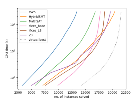
Figure 2: Plots showing the number of instances solved (x axis) within given time in seconds (y axis) in log scale.

Setup.

We have run our experiments on a cluster equipped with AMD EPYC 7502 CPUs running at 2.5GHz, using a timeout of 300 seconds, and a memory limit of 8GB. We have compared the base version of Yices2 with the LS-boosted version $\textsc{Yices2}_{LS}$ as well as with the state-of-the-art SMT solvers cvc5 [1] (version 1.2.0), MathSAT5 [11] (version 5.6.11), and Z3 [14] (version 4.13.3). We have also included in the comparison HybridSMT [7], which runs a portfolio composed by the LS solver LocalSMT [6] (used as a standalone tool) and a LocalSMT-boosted version of Z3’s CDCL(T) – see also related work (Section 6).

Benchmarks.

We have considered all the SMT-LIB [2] (Version 2024 [42]) benchmarks from the QF_NIA category. This is a class of 25443 benchmarks, among which 14990 and 5183 come with a known status of “sat” and “unsat”, respectively. Another 5270 have an “unknown” satisfiability status.

Results.

In the presentation of the results, we consider both a short time limit and a long time limit. We set the short time limit to 24s, as in the respective SMT-COMP track [45], and the long time limit to 300s, due to resource constraints. The results are shown in Table 1 and Table 2, respectively. In the columns, we separate per benchmark family; on the rows, for each solver, we report the amount of overall benchmarks solved, and, in parenthesis, the amount of benchmarks solved restricted to sat and unsat instances, respectively. We also include two portfolios between Z3 (resp., HybridSMT) and $\textsc{Yices2}_{LS}$, that work as follows: we run Z3 (resp., HybridSMT) for half of the time limit (i.e., 12s/150s), then, if it has not terminated, we run $\textsc{Yices2}_{LS}$ for the remaining time.

Discussion.

First, we observe that, with both time limits, $\textsc{Yices2}_{LS}$ solves a significant number of benchmarks more than $\textsc{Yices2}_{base}$. In particular, on both satisfiable and unsatisfiable instances, it improves (or matches) $\textsc{Yices2}_{base}$ results over all families, except one. Improving on unsatisfiable benchmarks is noteworthy: indeed, while, in general, local search is geared toward proving satisfiability, integrating it within MCSat enables to generate better lemmas. This is witnessed not only by the higher amount of benchmarks solved overall, but also by the lower amount of conflicts occurred: on unsatisfiable benchmarks solved by both tools, on average (resp. median), $\textsc{Yices2}_{LS}$ encountered 225 (resp. 4) conflicts less than $\textsc{Yices2}_{base}$. Note that, on average (resp. median), $\textsc{Yices2}_{base}$ encountered 1669 (resp. 458) conflicts. These numbers show that there is a considerable amount of benchmarks for which the number of conflicts is significantly lower (note that such a lower median w.r.t. average implies a pronounced right-skewness).

Overall, we see that, in the 24s track, $\textsc{Yices2}_{LS}$ solves more benchmarks than any other solver, while, in the 300s track, it comes third, after HybridSMT and Z3. The complementarity of $\textsc{Yices2}_{LS}$ w.r.t. both tools can be witnessed by the scatter plots in Figure 3, and by the results of the portfolios in Tables 1 and 2. Note that Z3 internally utilizes portfolio tactics that combine multiple solving techniques sequentially (clearly observable in Figures 2 and 3). HybridSMT runs a higher-level portfolio that combines the LS-based LocalSMT and Z3. The results of the portfolios that include $\textsc{Yices2}_{LS}$ show that our approach brings significant diversity to the strategies already used in state-of-the-art portfolio approaches. Since HybridSMT is the only other solver that – to the best of our knowledge – leverages local search techniques for $\mathcal{NIA}$, it is interesting to compare the improvements it brings to Z3 with the improvements that $\textsc{Yices2}_{LS}$ brings over $\textsc{Yices2}_{base}$. We can see that, with a 300s time limit, the improvements are comparable, as both tools solve around 800 benchmarks more than their base solvers. With a 24s time limit, however, we see that $\textsc{Yices2}_{LS}$ is able to solve around 700 benchmarks more than $\textsc{Yices2}_{base}$, while, on the contrary, HybridSMT loses around 450 benchmarks compared to Z3. Figure 2 shows that the point at which using local search pays off is much earlier for $\textsc{Yices2}_{LS}$ ($<10s$) than for HybridSMT (just below $100s$).

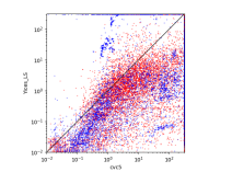
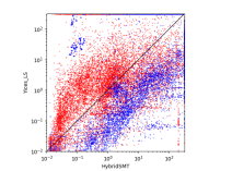
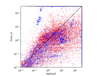
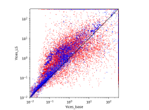
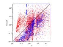
Figure 3: Scatter plots comparing $\textsc{Yices2}_{LS}$ to cvc5, HybridSMT, MathSAT5, $\textsc{Yices2}_{base}$, and Z3, respectively; on satisfiable (red) and unsat. (blue) instances.

6 Related work

In propositional SAT solving, local search techniques have been successfully used to solve difficult satisfiable problems [30] as well as unsatisfiable instances [43]. Recently, their tight integration in the propositional CDCL framework has been shown to improve performance [7, 8] and are now considered a key component of state-of-the-art SAT solvers. In the context of SMT, on the other hand, the adoption of LS is a lot less widespread.

In [22], the LS-based SAT solver WalkSAT has been used in combination with a theory solver as an alternative to the classic CDCL(T) approach; however, the use of local search remained limited to the Boolean level. For the theory of bit-vectors, the idea of Boolean flips in SAT solving has been transposed to the bit level by introducing bit-flips moves [18], possibly augmented with propagations [39].

The adoption of LS for arithmetic theories is more recent. For the theories of Linear Integer Arithmetic ($\mathcal{LIA}$) [5] and Multi-linear Real Arithmetic [33] a critical move operation is used to change the value of a variable that appears in a literal violated by the current assignment in order to make the literal satisfied. To deal with the nonlinear arithmetic constraints, the cell-jumping technique is used, which first isolates the roots of a falsified polynomial w.r.t. to a variable (by fixing the value of the other variables), thus decomposing the real space into finitely many intervals (cells, in the CAD [12] terminology), and then tries to satisfy the polynomial by changing the value of the variable by jumping around these cells. This technique has been implemented in LocalSMT for $\mathcal{NIA}$ [6], and as a tool in Maple [34] and on top of Z3 [44] for $\mathcal{NRA}$.

Local search has also been used as a sub-routine for global search techniques, as in the case of floating points  [19], and of $\mathcal{NRA}$ possibly augmented with transcendental functions ($\mathcal{N\mkern-1.0muT\mkern-4.0muA}$) [36, 37, 35]. In these works, numerical optimization algorithms, e.g. the gradient-descent, are used to find local minima, while stochastic jumping is used to move away from a local minimum in order to explore other regions in search for a global minimum.

All the methods discussed so far for arithmetic theories are only able to prove satisfiability; if they fail, then all the knowledge that has been acquired by the search is lost. HybridSMT [46] addresses this issue, for the case of $\mathcal{NIA}$, by integrating LocalSMT within Z3’s CDCL(T). In particular, LocalSMT takes as input a subformula corresponding to a Boolean skeleton solution, and, if it does not find an integer solution for the subformula, it returns the best assignment found and the conflict frequency for atoms. This information is used to improve phase selection (i.e. Boolean assignments) and variable ordering. Although both HybridSMT and our method share the idea of integrating LS within a reasoning calculus (CDCL(T) and MCSat, respectively), there are some substantial difference. First, in HybridSMT, LS takes into account complete Boolean variable assignments. In our framework, LS can take as input both Boolean and theory variable assignments, either partial or complete. Additionally, while in HybridSMT LS can only suggest assignments for (and ordering of) Boolean literals, we extend that to theory variables as well. Moreover, there is a theory-specific difference in our approach. LocalSMT relies on cell-jumps, which require to perform potentially very expensive root isolation sub-routines at every step. In contrast, our method uses fs-jumps that rely on feasibility intervals already maintained by the theory plugin in the MCSat framework. This eliminates the need for additional computation and can be viewed as a lazy version of cells, progressively refined on-demand. Furthermore, we pair fs-jumps with hill-climbing to move inside feasible intervals.

Most state-of-the-art solvers do not use local search for $\mathcal{NIA}$ problems. Bit-blasting [20] aims at proving satisfiability by iteratively imposing bounds on the variables and then encoding the obtained sub-formula into an equi-satisfiable Boolean formula, which is then handled by a SAT solver. In the branch-and-bound approach [31, 27] the integer domain is relaxed by allowing variables to range over real numbers. Incremental Linearization [9, 10] leverages decision procedures for $\mathcal{LIA}$ by abstracting non-linear multiplications with uninterpreted functions and then incrementally axiomatize them.

7 Conclusion

In this work, we have presented a theory-independent framework to integrate local search into the MCSat calculus, combining local search intuition with MCSat reasoning capabilities. In particular, we tackled the theory of nonlinear integer arithmetic by proposing a local search procedure based on feasibility-set jumping and hill-climbing. We implemented our approach in the Yices2 SMT solver, and empirically demonstrated its improvements for both satisfiable and unsatisfiable instances. Our results show that the new Yices2 solver with local search compares favorably and often outperforms other SMT solvers; in particular, it manages to solve a significant amount of benchmarks not solved by other state-of-the-art tools. In the future, we plan to extend our approach to other theories, particularly finite fields and bit-vectors, and conduct a more extensive experimental evaluation.

7.0.1 Acknowledgements

This material is based upon work supported in part by NSF grant 2016597. Any opinions, findings and conclusions or recommendations expressed in this material are those of the author(s) and do not necessarily reflect the views of the US Government or NSF.

7.0.2

The authors have no competing interests to declare that are relevant to the content of this article.

References

- [1] Haniel Barbosa, Clark W. Barrett, Martin Brain, Gereon Kremer, Hanna Lachnitt, Makai Mann, Abdalrhman Mohamed, Mudathir Mohamed, Aina Niemetz, Andres Nötzli, Alex Ozdemir, Mathias Preiner, Andrew Reynolds, Ying Sheng, Cesare Tinelli, and Yoni Zohar. cvc5: A versatile and industrial-strength SMT solver. In Dana Fisman and Grigore Rosu, editors, Tools and Algorithms for the Construction and Analysis of Systems - 28th International Conference, TACAS 2022, Held as Part of the European Joint Conferences on Theory and Practice of Software, ETAPS 2022, Munich, Germany, April 2-7, 2022, Proceedings, Part I, volume 13243 of Lecture Notes in Computer Science, pages 415–442. Springer, 2022.
- [2] Clark Barrett, Pascal Fontaine, and Cesare Tinelli. The Satisfiability Modulo Theories Library (SMT-LIB). www.SMT-LIB.org, 2016.
- [3] Clark W. Barrett, Roberto Sebastiani, Sanjit A. Seshia, and Cesare Tinelli. Satisfiability modulo theories. In Armin Biere, Marijn Heule, Hans van Maaren, and Toby Walsh, editors, Handbook of Satisfiability - Second Edition, volume 336 of Frontiers in Artificial Intelligence and Applications, pages 1267–1329. IOS Press, 2021.
- [4] Nikolaj Bjørner and Lev Nachmanson. Arithmetic solving in z3. In Arie Gurfinkel and Vijay Ganesh, editors, Computer Aided Verification, pages 26–41, Cham, 2024. Springer Nature Switzerland.
- [5] Shaowei Cai, Bohan Li, and Xindi Zhang. Local search for smt on linear integer arithmetic. In Sharon Shoham and Yakir Vizel, editors, Computer Aided Verification, pages 227–248, Cham, 2022. Springer International Publishing.
- [6] Shaowei Cai, Bohan Li, and Xindi Zhang. Local search for satisfiability modulo integer arithmetic theories. ACM Trans. Comput. Logic, 24(4), July 2023.
- [7] Shaowei Cai and Xindi Zhang. Deep cooperation of cdcl and local search for sat. In Chu-Min Li and Felip Manyà, editors, Theory and Applications of Satisfiability Testing – SAT 2021, pages 64–81, Cham, 2021. Springer International Publishing.
- [8] Shaowei Cai, Xindi Zhang, Mathias Fleury, and Armin Biere. Better decision heuristics in cdcl through local search and target phases. J. Artif. Int. Res., 74, September 2022.
- [9] Alessandro Cimatti, Alberto Griggio, Ahmed Irfan, Marco Roveri, and Roberto Sebastiani. Experimenting on solving nonlinear integer arithmetic with incremental linearization. In Olaf Beyersdorff and Christoph M. Wintersteiger, editors, Theory and Applications of Satisfiability Testing – SAT 2018, pages 383–398, Cham, 2018. Springer International Publishing.
- [10] Alessandro Cimatti, Alberto Griggio, Ahmed Irfan, Marco Roveri, and Roberto Sebastiani. Incremental linearization for satisfiability and verification modulo nonlinear arithmetic and transcendental functions. ACM Trans. Comput. Logic, 19(3), aug 2018.
- [11] Alessandro Cimatti, Alberto Griggio, Bastiaan Schaafsma, and Roberto Sebastiani. The MathSAT5 SMT Solver. In Nir Piterman and Scott Smolka, editors, Proceedings of TACAS, volume 7795 of LNCS. Springer, 2013.
- [12] George E. Collins. Quantifier elimination for real closed fields by cylindrical algebraic decompostion. In H. Brakhage, editor, Automata Theory and Formal Languages, pages 134–183, Berlin, Heidelberg, 1975. Springer Berlin Heidelberg.
- [13] Florian Corzilius, Gereon Kremer, Sebastian Junges, Stefan Schupp, and Erika Ábrahám. SMT-RAT: An open source C++ toolbox for strategic and parallel SMT solving. In SAT, 09 2015.
- [14] Leonardo De Moura and Nikolaj Bjørner. Z3: An efficient SMT solver. In Proceedings of the Theory and Practice of Software, 14th International Conference on Tools and Algorithms for the Construction and Analysis of Systems, TACAS’08/ETAPS’08, page 337–340, Berlin, Heidelberg, 2008. Springer-Verlag.
- [15] Leonardo de Moura and Dejan Jovanovic. A model-constructing satisfiability calculus. In Roberto Giacobazzi, Josh Berdine, and Isabella Mastroeni, editors, Intl. Conference on Verification, Model Checking, and Abstract Interpretation (VMCAI), volume 7737 of LNCS, pages 1–12. Springer, 2013.
- [16] Leonardo Mendonça de Moura and Nikolaj S. Bjørner. Satisfiability modulo theories: introduction and applications. Commun. ACM, 54(9):69–77, 2011.
- [17] Bruno Dutertre. Yices 2.2. In Armin Biere and Roderick Bloem, editors, Computer-Aided Verification (CAV’2014), volume 8559 of Lecture Notes in Computer Science, pages 737–744. Springer, July 2014.
- [18] Andreas Fröhlich, Armin Biere, Christoph Wintersteiger, and Youssef Hamadi. Stochastic local search for satisfiability modulo theories. Proceedings of the AAAI Conference on Artificial Intelligence, 29(1), Feb. 2015.
- [19] Zhoulai Fu and Zhendong Su. Xsat: A fast floating-point satisfiability solver. In CAV, volume 9780 of Lecture Notes in Computer Science, pages 187–209. Springer, 2016.
- [20] Carsten Fuhs, Jürgen Giesl, Aart Middeldorp, Peter Schneider-Kamp, René Thiemann, and Harald Zankl. Sat solving for termination analysis with polynomial interpretations. In João Marques-Silva and Karem A. Sakallah, editors, Theory and Applications of Satisfiability Testing – SAT 2007, pages 340–354, Berlin, Heidelberg, 2007. Springer Berlin Heidelberg.
- [21] Stéphane Graham-Lengrand, Dejan Jovanovic, and Bruno Dutertre. Solving bitvectors with MCSAT: explanations from bits and pieces. In Nicolas Peltier and Viorica Sofronie-Stokkermans, editors, Intl. Joint Conf. on Automated Reasoning (IJCAR), Part I, volume 12166 of LNCS, pages 103–121. Springer, 2020.
- [22] Alberto Griggio, Quoc-Sang Phan, Roberto Sebastiani, and Silvia Tomasi. Stochastic local search for smt: Combining theory solvers with walksat. In Cesare Tinelli and Viorica Sofronie-Stokkermans, editors, Frontiers of Combining Systems, pages 163–178, Berlin, Heidelberg, 2011. Springer Berlin Heidelberg.
- [23] Thomas Hader, Daniela Kaufmann, Ahmed Irfan, Stéphane Graham-Lengrand, and Laura Kovács. MCSat-based finite field reasoning in the yices2 SMT solver (short paper). In IJCAR (1), volume 14739 of Lecture Notes in Computer Science, pages 386–395. Springer, 2024.
- [24] Thomas Hader, Daniela Kaufmann, and Laura Kovács. SMT solving over finite field arithmetic. In LPAR, volume 94 of EPiC Series in Computing, pages 238–256. EasyChair, 2023.
- [25] Leticia Hernando, Alexander Mendiburu, and Jose Lozano. Hill-climbing algorithm: Let’s go for a walk before finding the optimum. pages 1–7, 07 2018.
- [26] Ahmed Irfan and Stéphane Graham-Lengrand. Arrays reasoning in MCSat. In SMT@CAV, volume 3725 of CEUR Workshop Proceedings, pages 24–35. CEUR-WS.org, 2024.
- [27] Dejan Jovanović. Solving nonlinear integer arithmetic with mcsat. In Ahmed Bouajjani and David Monniaux, editors, Verification, Model Checking, and Abstract Interpretation, pages 330–346, Cham, 2017. Springer International Publishing.
- [28] Dejan Jovanovic, Clark Barrett, and Leonardo de Moura. The design and implementation of the model constructing satisfiability calculus. In Intl. Conf on Formal Methods in Computer-Aided Design (FMCAD), pages 173–180. IEEE, 2013.
- [29] Dejan Jovanović and Leonardo de Moura. Solving non-linear arithmetic. ACM Commun. Comput. Algebra, 46(3/4):104–105, jan 2013.
- [30] Henry A. Kautz, Ashish Sabharwal, and Bart Selman. Incomplete algorithms. In Armin Biere, Marijn Heule, Hans van Maaren, and Toby Walsh, editors, Handbook of Satisfiability - Second Edition, volume 336 of Frontiers in Artificial Intelligence and Applications, pages 213–232. IOS Press, 2021.
- [31] Gereon Kremer, Florian Corzilius, and Erika Ábrahám. A generalised branch-and-bound approach and its application in SAT modulo nonlinear integer arithmetic. In Vladimir P. Gerdt, Wolfram Koepf, Werner M. Seiler, and Evgenii V. Vorozhtsov, editors, Computer Algebra in Scientific Computing - 18th International Workshop, CASC 2016, Bucharest, Romania, September 19-23, 2016, Proceedings, volume 9890 of Lecture Notes in Computer Science, pages 315–335. Springer, 2016.
- [32] Gereon Kremer and Erika Ábrahám. Modular strategic smt solving with smt-rat. Acta Universitatis Sapientiae, Informatica, 10(1):5–25, 2018.
- [33] Bohan Li and Shaowei Cai. Local search for smt on linear and multi-linear real arithmetic. In 2023 Formal Methods in Computer-Aided Design (FMCAD), pages 1–10, 2023.
- [34] Haokun Li, Bican Xia, and Tianqi Zhao. Local search for solving satisfiability of polynomial formulas. In Constantin Enea and Akash Lal, editors, Computer Aided Verification, pages 87–109, Cham, 2023. Springer Nature Switzerland.
- [35] Enrico Lipparini. Satisfiability modulo Nonlinear Arithmetic and Transcendental Functions via Numerical and Topological methods. PhD thesis, 2024.
- [36] Enrico Lipparini, Alessandro Cimatti, Alberto Griggio, and Roberto Sebastiani. Handling polynomial and transcendental functions in SMT via unconstrained optimisation and topological degree test. In Ahmed Bouajjani, Lukáš Holík, and Zhilin Wu, editors, Automated Technology for Verification and Analysis, pages 137–153, Cham, 2022. Springer International Publishing.
- [37] Enrico Lipparini and Stefan Ratschan. Satisfiability of non-linear transcendental arithmetic as a certificate search problem. J. Autom. Reason., 69(1), January 2025.
- [38] Yuri V. Matiyasevich. Hilbert’s tenth problem. MIT Press, Cambridge, MA, USA, 1993.
- [39] Aina Niemetz, Mathias Preiner, and Armin Biere. Propagation based local search for bit-precise reasoning. Formal Methods in System Design, 51(3):608–636, Dec 2017.
- [40] Robert Nieuwenhuis, Albert Oliveras, and Cesare Tinelli. Solving sat and sat modulo theories: From an abstract davis–putnam–logemann–loveland procedure to dpll(t). J. ACM, 53(6):937–977, November 2006.
- [41] Knot Pipatsrisawat and Adnan Darwiche. A lightweight component caching scheme for satisfiability solvers. In Theory and Applications of Satisfiability Testing–SAT 2007: 10th International Conference, Lisbon, Portugal, May 28-31, 2007. Proceedings 10, pages 294–299. Springer, 2007.
- [42] Mathias Preiner, Hans-Jörg Schurr, Clark Barrett, Pascal Fontaine, Aina Niemetz, and Cesare Tinelli. SMT-LIB release 2024 (non-incremental benchmarks), April 2024.
- [43] Steven Prestwich and Inês Lynce. Local search for unsatisfiability. In Armin Biere and Carla P. Gomes, editors, Theory and Applications of Satisfiability Testing - SAT 2006, pages 283–296, Berlin, Heidelberg, 2006. Springer Berlin Heidelberg.
- [44] Zhonghan Wang, Bohua Zhan, Bohan Li, and Shaowei Cai. Efficient local search for nonlinear real arithmetic. In Rayna Dimitrova, Ori Lahav, and Sebastian Wolff, editors, Verification, Model Checking, and Abstract Interpretation, pages 326–349, Cham, 2024. Springer Nature Switzerland.
- [45] Tjark Weber, Sylvain Conchon, David Déharbe, Matthias Heizmann, Aina Niemetz, and Giles Reger. The SMT competition 2015-2018. J. Satisf. Boolean Model. Comput., 11(1):221–259, 2019.
- [46] Xindi Zhang, Bohan Li, and Shaowei Cai. Deep combination of cdcl(t) and local search for satisfiability modulo non-linear integer arithmetic theory. In Proceedings of the IEEE/ACM 46th International Conference on Software Engineering, ICSE ’24, New York, NY, USA, 2024. Association for Computing Machinery.