Cosmological phase-space analysis of $f(G)$-theories of gravity

Abstract

The impact of topological terms that modify the Hilbert-Einstein action is here explored by virtue of a further $f(G)$ contribution. In particular, we investigate the phase-space stability and critical points of an equivalent scalar field representation that makes use of a massive field, whose potential is function of the topological correction. To do so, we introduce to the gravitational Action Integral a Lagrange multiplier and model the modified Friedmann equations by virtue of new non-dimensional variables. We single out dimensionless variables that permit a priori the Hubble rate change of sign, enabling regions in which the Hubble parameter either vanishes or becomes negative. In this respect, we thus analyze the various possibilities associated with a universe characterized by such topological contributions and find the attractors, saddle points and regions of stability, in general. The overall analysis is carried out considering the exponential potential first and then shifting to more complicated cases, where the underlying variables do not simplify. We compute the eigenvalues of our coupled differential equations and, accordingly, the stability of the system, in both a spatially-flat and non-flat universe. Quite remarkably, regardless of the spatial curvature, we show that a stable de Sitter-like phase that can model current time appears only a small fraction of the entire phase-space, suggesting that the model under exam is unlikely in describing the whole universe dynamics, i.e., the topological terms appear disfavored in framing the entire evolution of the universe.

I Introduction

Challenging General Relativity has acquired much more attention in view of the most recent cosmological observations that certify the existence of a dark sector 2006IJMPD..15.1753C ; Gruber:2013wua ; delaCruz-Dombriz:2016bqh ; Sahni:2006pa ; Dunsby:2016lkw , fully-unknown, albeit necessary for both clustering and accelerating the universe Bamba:2012cp ; 2001IJMPD..10..213C ; 2003PhRvL..90i1301L . Accordingly, conceptual limitations or experimental drawbacks are becoming gradually more explored Simon2005 , especially in strong gravitational fields 2020A&A…641A.174L ; 2021MNRAS.503.4581L , where gravity breaks down Kiefer:2023bld or a non-trivial mechanism of vacuum energy production is expected Martin:2012bt leading to the cosmological constant problem Luongo:2018lgy ; Belfiglio:2022qai ; Luongo:2023aaq and so on.

The advantage of extending the Hilbert-Einstein’s action lies on the fact that Einstein’s theory is not renormalizable 2003PhR…380..235P ; 1992ARA&A..30..499C and, in turn, cannot be conventionally quantized. The cosmological constant problem, for example, remains an open challenge of our current understanding weinberg1989cosmological ; Luongo:2018lgy ; Capozziello:2025bsm and limits the possibility to characterize the cosmological constant today, as experimentally found 2024A&A…690A..40L ; Khadka:2021vqa ; Luongo:2021nqh ; Dunsby:2015ers ; Vilardi:2024cwq ; Bamba:2012cp ; Capozziello:2021xjw .

To face this problem the renormalization at one loop requires the Einstein-Hilbert action to be supplemented with additional higher-order curvature terms that, however, turn out to be generally not unitary. Analogously, when quantum corrections, for example under the form of string modifications, are included, the effective low-energy gravitational action naturally incorporates higher-order curvature invariants, leading to experimental signature in extremely strong gravity regimes such as cosmological Planck scale, black hole singularities, etc.

However, signatures of this picture may be found even at the level of infrared scales, providing evidences in favor of modifying Einstein’s gravity at all scales.

A natural extension of Einstein’s gravity may lead to $f(R)$ theories of gravity Sotiriou:2008rp ; Nojiri:2008nk ; Nojiri:2008nt , constructed as analytic functions of Ricci scalar $R$, whose prototype is offered by a second order term, $\propto R^{2}$, named scalaron Starobinsky:1980te . Viable $f(R)$ models, fulfilling both cosmological and local gravity constraints, have not really been found so far, and, in general, the matter sector is mainly coupled with such theories, limiting the consistency with observations.

Going through these paradigms, in view of the large number of proposals, one can find theories with a Lagrangian density being a combination of terms Barrow:1988xh ; Barrow:1991hg ; Bueno:2016dol ; Lovelock:1971yv $R_{\mu\nu}R^{\mu\nu}$ and $R^{\mu\nu\rho\sigma}R_{\mu\nu\rho\sigma}$, namely superpositions of the Ricci and Riemann tensors, respectively, that however are jeopardized by unphysical spin-2 ghost instabilities. Analogously, for the sake of completeness, other approaches such as torsion Nesseris:2013jea ; Geng:2011aj ; Paliathanasis:2016vsw ; Duchaniya:2023aeu ; DAgostino:2018ngy or non-metricity Heisenberg:2023lru ; Koussour:2023rly ; Solanki:2022ccf ; Anagnostopoulos:2021ydo can, as well, provide hints on how to heal the aforementioned issue, see e.g. BeltranJimenez:2019esp .

In this respect and quite remarkably, we here single out the study of Gauss-Bonnet (GB) terms Padmanabhan:2013xyr ; Dotti:2007az ; Charmousis:2002rc ; Pozdeeva:2019agu , defined as, $G\equiv R^{2}-4R^{\mu\nu}R_{\mu\nu}+R_{\mu\nu\alpha\beta}R^{\mu\nu\alpha\beta}$, that can significantly improve the above picture.

Over the past decades, various studies have explored this topic, generally revealing that satisfying local gravity constraints remains challenging when the GB term is responsible for dark energy. However, this appears feasible for certain plausible $f(G)$ Lagrangians Nojiri:2005jg that yield a cosmological constant Li:2007jm ; Nojiri:2021mxf ; Nojiri:2024nlx ; Myrzakulov:2024sne ; Lohakare:2024ize ; Bamba:2017cjr ; Nojiri:2010wj; Nojiri:2017ncd; Nojiri:2018ouv.

Although a definitive conclusion on the validity of extended gravity, and specifically $f(G)$ models, has yet to be reached, investigating their stability and properties remains crucial for assessing their potential role in cosmology.

Motivated by the above considerations, we here focus on $f(G)$ theories of gravity and analyze the corresponding stability and phase-space dynamics. To do so, we limit our study to a FLRW background, reconsidering $f(G)$ theories as scalar field-equivalent representation, modifying the corresponding Lagrangian by including a Lagrangian multiplier. After computing the modified Friedmann equations, we formulate the cosmological dynamics by virtue of appropriate dynamical variables, rewritten in order to account for all possible behaviors of the universe, namely enabling the Hubble parameter to change sign, as a consequence of the dynamical prescription. The corresponding autonomous system of dynamical equations has been obtained and the computation of eigenvalues has been found. Analyzing then the phase-space we obtain the existence of attractors and explore the stability of each point under exam. Analogously the stability at asymptotic regime has been found. To do so, we employ a particular version of power-law potential and compare our findings with previous literature. As a matter of fact, we emphasize that the so-constructed model converges to a de Sitter phase

The paper is organized as follows. In Sect. II, we introduce the concepts related to $f(G)$ cosmology. The equivalent scalar field description is also reported in detail. The dynamical consequences, adopting the modified Friedmann equations, are reported in Sect. III. There, we also baptize our dynamical variables and set the system of differential equations, used throughout our work. The consequences on our observable universe are summarized in Sect. IV. There, we report the cases of spatially-flat and non-flat universe and the overall analysis. Finally, the scalar field potentials and their impact under the form of power-law contribution is explored in Sect. V, whereas our final outlooks and perspectives are summarized in Sect. VI.

II $f\left(G\right)$-Cosmology

At large scales, the maximally symmetric spacetime describing the universe is the four-dimensional isotropic and homogeneous Friedmann-Lemaitre-Robertson-Walker geometry,

$$ds^{2}=-N^{2}\left(t\right)dt^{2}+a^{2}\left(t\right)\left[\frac{dr^{2}}{1-kr^{2}}+r^{2}\left(d\theta^{2}+\sin^{2}\theta d\varphi^{2}\right)\right],$$ (1)

with $a\left(t\right)$ representing the cosmic scale factor, $N\left(t\right)$ the lapse function and $k$ denotes the spatial curvature of the associated three-dimensional hypersurface.

The latter indicates the universe topology, namely for $k=0$, the universe is spatially flat, while for $k=-1$, the hypersurface has negative curvature, turning out to be hyperbolic and, finally, $k=1$ leads to an hypersurface represented by a closed sphere.

For the gravitational theory, we assume the modified four-dimensional Gauss-Bonnet theory with the action, $S[R,G]=\int d^{4}x\sqrt{-g}\,\mathcal{L}[R,G]$, given by Li:2007jm

$$S[R,G]=\int d^{4}x\sqrt{-g}\left(R+f\left(G\right)\right),$$ (2)

where $f\left(G\right)$ is an arbitrary function of the Gauss-Bonnet scalar, $G$, and $R$ is the Ricci scalar, providing standard Einstein’s gravity.

As stated in the introduction, in a four-dimensional manifold, the Gauss-Bonnet scalar is a topological invariant, i.e., $G$ represents a boundary term, while considering any linear $f\left(G\right)$ function, de facto lets Eq. (2) turn into the equivalent Hilbert-Einstein action.

Accordingly, we hereafter focus on non-linear $f\left(G\right)$ contributions, with the aim of exploring its effects over the cosmic expansion history.

II.1 Scalar field equivalent description

Remarkably, introducing a Lagrange multiplier would easily provide an equivalent description in terms of scalar fields. Accordingly, we can show that the geometrodynamical degrees of freedom provided by the nonlinear function $f\left(G\right)$ can be mimicked with a scalar field.

Specifically, the gravitational model in Eq. (2) is equivalent to the Einstein-Gauss-Bonnet-Scalar field theory, where the scalar field is coupled to $G$.

Motivated by this recipe, we employ the Lagrange multiplier, $\lambda$, and write the Eq. (2) as

$$S_{f\left(G\right)}=\int d^{4}x\sqrt{-g}\left(R+f\left(G\right)-\lambda\left(G-\mathcal{G}\right)\right),$$ (3)

where, solving the equations of motion, leads to the constraint $G=\mathcal{G}$, that will be essential for our computation later on.

By varying the Lagrangian with respect to the Gauss-Bonnet term gives

$$\lambda=f_{,G}\left(G\right),$$ (4)

that permits to reformulate the Lagrangian by

$$\mathcal{L}=R+\left(f\left(G\right)-Gf_{,G}\left(G\right)\right)+f_{,G}\left(G\right)\mathcal{G}.$$ (5)

Conveniently, ensuring that $f(G)$ and $f_{,G}(G)$ are distinct variables, we can introduce the scalar field representation by

$$\phi=f_{,G}\left(G\right),$$ (6a)

$$V\left(\phi\right)=\left(f\left(G\right)-Gf_{,G}\left(G\right)\right),$$ (6b)

ending up with the equivalent Einstein-Gauss-Bonnet scalar field picture shown as

$$S_{f\left(G\right)}=\int d^{4}x\sqrt{-g}\left(\frac{R}{2}+\phi G+V\left(\phi\right)\right).$$ (7)

This is the Action Integral for the Einstein-Gauss-Bonnet Scalar field gravitational model Fomin:2018typ ; Odintsov:2020xji ; Paliathanasis:2024gwp ; Millano:2024vju ; TerenteDiaz:2023iqk ; Nojiri:2023jtf ; Hussain:2024yee without a kinetic term.

Afterwards, from the line element in Eq. (3), the Ricci, $R$, and the Gauss-Bonnet, $G$, scalars are

$$R=6\left(\frac{1}{N}\dot{H}+2H^{2}+\frac{k}{a^{2}}\right),$$ (8a)

$$G=24\left(\frac{1}{N}\dot{H}+H^{2}\right)\left(H^{2}+\frac{k}{a^{2}}\right),$$ (8b)

where we baptize the Hubble function, $H\equiv\frac{1}{N}\frac{\dot{a}}{a}$.

Hence, plugging the Ricci and Gauss-Bonnet scalars into Eq. (7) and, thus, integrating by parts, we obtain the following point-like Lagrangian,

$$\mathcal{L}\left(N,a,\dot{a},\phi,\dot{\phi}\right)=\frac{3}{N}a\dot{a}^{2}-\frac{8}{N^{3}}\dot{a}^{3}\dot{\phi}+3ka\left(N-\frac{8}{N}\frac{\dot{a}}{a}\dot{\phi}\right)+Na^{3}V\left(\phi\right),$$ (9)

from which it appears quite natural to compute the cosmological field equations with respect to the dynamical variables $\left\{N,a,\phi\right\}$. Specifically, the variation with respect to the lapse function, $N$, gives the constraint equation.

$$3H^{2}-24H^{3}\frac{\dot{\phi}}{N}-\frac{3k}{a^{2}}\left(1+8H\frac{\dot{\phi}}{N}\right)-V\left(\phi\right)=0,$$ (10)

while varying with respect to the scale factor, $a$, and to the scalar field, $\phi$, provides the following second-order (for $a(t)$ and $\phi$) differential equations,

$$\frac{1}{N}\dot{H}+H^{2}+\frac{V_{,\phi}}{24\left(H^{2}+\frac{k}{a^{2}}\right)}=0,$$ (11a)

$$\frac{12\ddot{\phi}}{N^{2}}\left(\frac{k}{a^{2}}+H^{2}\right)^{2}-3\left(\frac{k}{a^{2}}\right)^{2}+\left(3H^{4}+\frac{V_{,\phi}}{8}\right)-12\left(\frac{k}{a^{2}}+H^{2}\right)^{2}\left(\frac{3}{N}H+\frac{\dot{N}}{N^{3}}\right)-\frac{1}{8}\frac{\dot{\phi}}{N}HV_{,\phi}=0.$$ (11b)

Bearing these results in mind, we can accordingly compute the cosmological dynamics.

III Cosmological dynamics

We here work out a detailed phase-space analysis based on Eqs. (10), (11a) and (11b).

Enabling the Hubble rate to space over positive and negative regions, we can introduce the dimensionless variables Paliathanasis:2024gwp ; Millano:2024vju

$$x=8\frac{\dot{\phi}}{1+H^{2}},$$ (12a)

$$y^{2}=\frac{V\left(\phi\right)}{1+H^{2}},$$ (12b)

$$\eta=\frac{H}{\sqrt{\left(1+H^{2}\right)}},$$ (12c)

$$\omega_{k}=\frac{k}{a^{2}\left(1+H^{2}\right)},$$ (12d)

$$\lambda=\frac{V_{,\phi}}{V},$$ (12e)

$$\tau=\ln a,$$ (12f)

which differ from the $H$-normalization approach Copeland:2006wr since the assumption made through these parameters allows us to pass through $H=0$, i.e., to let $H$ change sign, as stated above.

Selecting $\tau$ as the new independent variable, the field equations turn into

$$\left(\eta^{4}+\left(1-\eta^{2}\right)\omega_{k}\right)^{2}\frac{dx}{d\tau} =-\frac{y\eta^{2}}{24}\left(1-\eta^{2}\right)\left(\eta^{2}\left(2\lambda-\eta\left(2\left(\lambda-12\right)\eta+\lambda x\left(2+\eta^{2}\right)\right)\right)\right)$$

$$-\frac{y\eta^{2}}{24}\left(1-\eta^{2}\right)^{2}\left(\lambda x\eta-24\right)\omega_{k}^{2}+\omega_{k}^{4}\left(1-\eta^{2}\right)^{2}\left(\eta^{2}\left(\eta x-1\right)-1\right)$$

$$+\left(\eta^{7}\left(\eta\left(1+\eta^{2}\left(\eta x-1\right)\right)-2x\left(1-\eta^{2}\right)\omega_{k}^{2}\right)\right),$$ (13)

$$\frac{dy}{d\tau}=-\frac{1}{48}y\sqrt{1-\eta^{2}}\left(3\lambda x+2\eta^{3}\left(24+\frac{\lambda y\left(1-\eta^{2}\right)}{\eta^{4}-\left(1-\eta^{2}\right)\omega_{k}}\right)\right),$$ (14)

$$\frac{d\eta}{d\tau}=\frac{y}{24\eta}\left(3\lambda x\eta+48\eta^{4}+2\lambda y\left(1-\eta^{2}\right)\right),$$ (15)

$$\frac{d\omega_{k}}{d\tau}=\frac{\left(1-\eta_{k}\right)^{2}}{12\eta}\omega_{k}^{2}\left(24+\frac{\lambda y\left(1-\eta^{2}\right)}{\eta^{4}-\left(1-\eta^{2}\right)\omega_{k}}\right),$$ (16)

and

$$\frac{d\lambda}{d\tau}=\frac{\lambda}{8}x\left(\Gamma\left(\lambda\right)-1\right),$$ (17)

where $\Gamma\left(\lambda\right)=\frac{V_{,\phi\phi}V}{\left(V_{,\phi}\right)^{2}}$.

Further, from Eq. (10) the algebraic constraint follows

$$\frac{1}{3}y+\omega_{k}-\eta^{2}+\frac{\eta}{1-\eta^{2}}x\left(\eta^{2}+\omega_{k}\right)=0.$$ (18)

By construction, $\eta$ is limited as $\eta^{2}\leq 1$, although the other variables are not compactified. Indeed, for $\eta^{2}=1$, the solution describes a scaling universe, while for $\eta^{2}<1$, the solution describes a de Sitter solution. Nevertheless, when $\eta>0$ the dynamical system describes an expanding universe $\left(H>0\right)$, while for $\eta<0$, the dynamical system describes a collapsing universe $\left(H<0\right)$.

In terms of the dimensionless variables the deceleration parameter $q=-1-\frac{\dot{H}}{H^{2}}$ 2016IJGMM..1330002D ; 2012PhRvD..86l3516A ; 2014PhRvD..90d3531A ; 2017PDU….17…25A ; 2024A&A…690A..40L ; 2020A&A…641A.174L is expressed as

$$q\left(x,y,\eta,\omega_{k}\right)=\frac{\lambda}{24}\frac{1-\eta^{2}}{\eta^{2}}\frac{y}{\eta^{2}+\omega_{k}}.$$ (19)

Immediately we remark that,

• The field equations form a five-dimensional dynamical system of first-order differential equations. By using the constraint provided in Eq. (18), the dimension of the dynamical system is reduced by one.

• Moreover, for the exponential potential $V\left(\phi\right)=V_{0}e^{\lambda_{0}\phi}$, it follows that $\Gamma\left(\lambda\right)-1=0$, thus, parameter $\lambda$ is always a constant, i.e. $\lambda=\lambda_{0}.$

• Hence, in order to reduce further the dimension of the dynamical system we consider the exponential potential.

  Indeed, for the exponential potential $V\left(\phi\right)$, the corresponding $f\left(G\right)$ function is derived

  $$f\left(G\right)=\frac{G}{\lambda_{0}}\left[\ln\left(-\frac{G}{\lambda_{0}V_{0}}\right)-1\right].$$ (20)

IV Consequences on the observable Universe

We can now wonder whether our scenario can be matched with the observable universe. This would be important in order to check the goodness of our approach and to infer limits about the initial Lagrangian, proposed in Eq. (3). To do so, we focus below on spatially-flat and non-flat universe and find the possible attractors and stability at infinity.

IV.1 Spatially-flat universe

Consider now a spatially flat FLRW universe, $k=0$, rewriting $y$ from Eq. (18), the two-dimensional system yields, $\left\{x,\eta\right\}$, that is,

$$\frac{dx}{d\tau}=1-\eta^{2}\left(1-x\eta\right)-\frac{\left(\eta\left(x+\eta\right)-1\right)\left(\lambda x\eta\left(2+\eta^{2}\right)-2\lambda+2\eta^{2}\left(\lambda-12\right)\right)}{8\eta^{2}},$$ (21)

$$\frac{d\eta}{d\tau}=-\frac{1}{24}\eta^{2}\left(1-\eta^{2}\right)\left(24+\frac{\lambda\eta^{2}\left(1-\eta^{2}\right)\left(1-x\eta+\eta^{2}\right)}{1-\eta^{2}}\right).$$ (22)

The stationary/equilibrium points $A=\left(x\left(A\right),\eta\left(A\right)\right)$ of the latter two-dimensional system are

$$A_{1} =\left(0,1\right),~A_{2}=\left(0,-1\right),~$$

$$A_{3} =\left(\frac{32}{3}\frac{1}{\lambda},1\right)~,~A_{4}=\left(-\frac{32}{3}\frac{1}{\lambda},-1\right),$$

$$A_{5} =\left(0,\sqrt{\frac{\lambda}{\lambda-8}}\right),~A_{6}=\left(0,-\sqrt{\frac{\lambda}{\lambda-8}}\right).$$

The equilibrium points with odd numbers describe expanding universes, while the equilibrium points with even numbers describe collapse. Points $A_{5}$, $A_{5}$ describe de Sitter solutions, while the remaining points describe scaling exact solutions.

In particular, the equilibrium points $A_{1}$, $A_{2}$ describe asymptotic solutions with deceleration parameters $q\left(A_{1}\right)=0,~$ $q\left(A_{2}\right)=0$. The Gauss-Bonnet term contributes in the cosmic fluid, and $y\left(A_{1}\right)=3,~y\left(A_{2}\right)=3$. As far as the stability of the points is concerned, we determine that the eigenvalues of the linearized system around point $A_{1}$ are $\left\{4,2\right\}$, and for point $A_{2}$ they are $\left\{-4,-2\right\}$. Thus point $A_{1}$ is always a source and point $A_{2}$ is always an attractor.

Equilibrium points $A_{3}$ and $A_{4}$ describe scaling solutions which can describe cosmic acceleration, that is, $q\left(A_{3}\right)=-\frac{4}{3}$ and $q\left(A_{4}\right)=-\frac{4}{3}$. At these points parameter $y$ reaches infinity. The eigenvalues for point $A_{3}$ are $\left\{-4,-\frac{2}{3}\right\}$, while for point $A_{4}$ are derived $\left\{4,\frac{2}{3}\right\}$. Therefore, point $A_{3}$ is always an attractor and point $A_{4}$ is always a source point.

Furthermore, equilibrium points $A_{5}$ and $A_{6}$ describe de Sitter solutions with $q\left(A_{5}\right)=-1$, and $q\left(A_{6}\right)=-1$. The points are real for $\lambda<0.$ At these points there is a nonzero contribution of the scalar field potential, that is, $y=\frac{3\lambda}{\lambda-8}$. The eigenvalues of the linearized systems around these points are $\left\{-\frac{3+\sqrt{17}}{2}\sqrt{\frac{\lambda}{\lambda-8}},-\frac{3-\sqrt{17}}{2}\sqrt{\frac{\lambda}{\lambda-8}}\right\}$, from where we conclude that the equilibrium points are always saddle points.

IV.1.1 Analysis at infinity

Above, we computed the equilibrium points for the dynamical system, reported in Eqs. (21) and (22), in the finite regime.

Nevertheless, clarifying the asymptotic regime appears quite interesting, as the variable $x$ can acquire values at infinity.

Accordingly, we thus introduce the new compactified variable, $X$, so that $x=\frac{X}{\sqrt{1-X^{2}}}$ and study the existence of equilibrium points at infinity, where $X^{2}=1$.

Indeed, there are four points, $\hat{A}=\left(X\left(\hat{A}\right),\eta\left(\hat{A}\right)\right),$ with coordinates

$$\hat{A}_{1}^{\pm}=\left(\pm 1,1\right)~,~\hat{A}_{2}^{\pm}=\left(\pm 1,-1\right).$$

At these points we calculate the deceleration parameter $q\left(\hat{A}_{1}^{\pm}\right)=-sign\left(\lambda X\left(\hat{A}_{1}^{\pm}\right)\right)\infty$ and $q\left(\hat{A}_{2}^{\pm}\right)=sign\left(\lambda X\left(\hat{A}_{2}^{\pm}\right)\right)\infty$. Points $\hat{A}_{1}^{\pm}$ describe an expanding universes, but for $sign\left(\lambda X\left(\hat{A}_{1}^{\pm}\right)\right)<0,$ we derive that $q\left(\hat{A}_{1}^{\pm}\right)>0$, that means these stationary points correspond to asymptotic solutions, asymptotically reaching the Minkowski space.

The same holds for the points exhibiting $sign\left(\lambda X\left(\hat{A}_{2}^{\pm}\right)\right)<0$.

Consequently, the existence of these stationary points is essential in order the cosmological evolution to cross from expansion to collapse and vice versa. Recall that $\eta=0$, gives a singularity at the dynamical system, so the transition is happening through the points at infinity.

This prescription is explicitly reported in Fig. 1. Last but not least, the stationary points at infinity always correspond to unstable solutions.

From the phase-space portraits displayed in Fig. 1, it appears clear that the most of underlying initial conditions leads to a collapsed universe, whereas only a small fraction of the entire phase-space, less than one quarter, corresponds to trajectories with initial conditions leading to a future attractor and, then, describing cosmic acceleration.

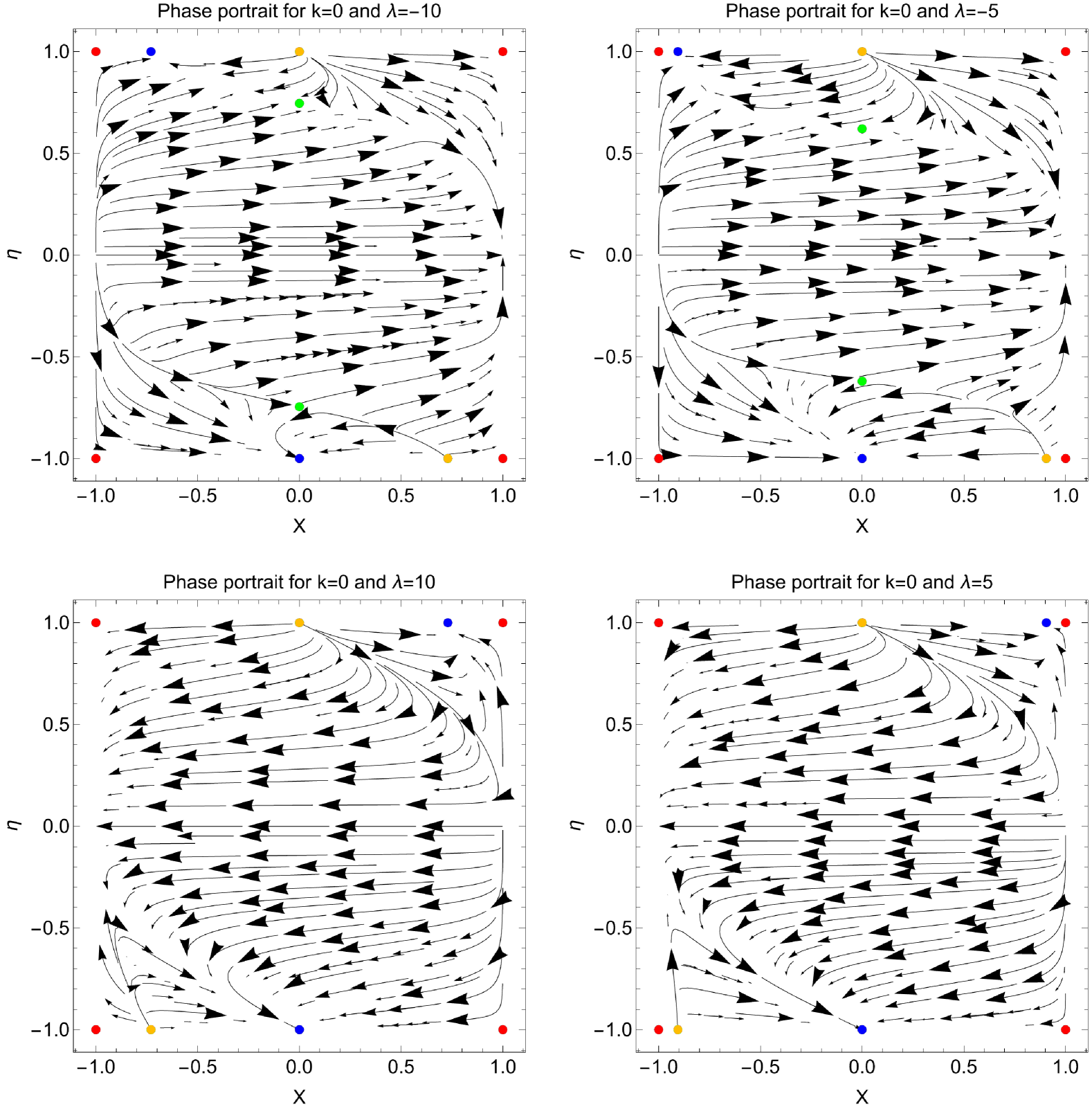
Figure 1: Phase-space portrait for the dynamical system (21), (22) in the compactified variables $X$ and $\eta$. Equilibrium points at the infinity are marked with red, the source points $A_{1}$ and $A_{4}$ are marked with orange, the saddle points $A_{5}$ and $A_{6}$ with green, and the attractors $A_{2}$ and $A_{5}$ are marked with blue. We observe that the main of the initial conditions lead to a collapsed universe, while there exist only a small area, less than then one quarter, of the phase-space, where the trajectories lead to a future attractor which describes cosmic acceleration.

A summary of the above outcomes is summarized in Table 1.

Table 1: Equilibrium Points for the spatially flat FLRW universe and exponential potential.

Point	$\left(\mathbf{x,\eta}\right)$	Existence	$q$	Stable?
$A_{1}$	$\left(0,1\right)$	Always	$0$	False
$A_{2}$	$\left(0,-1\right)$	Always	$0$	Attractor
$A_{3}$	$\left(\frac{32}{3}\frac{1}{\lambda},1\right)$	$\lambda\neq 0$	$-\frac{4}{3}$	Attractor
$A_{4}$	$\left(-\frac{32}{3}\frac{1}{\lambda},-1\right)$	$\lambda\neq 0$	$-\frac{4}{3}$	False
$A_{5}$	$\left(0,\sqrt{\frac{\lambda}{\lambda-8}}\right)$	$\lambda<0$	$-1$	False
$A_{6}$	$\left(0,-\sqrt{\frac{\lambda}{\lambda-8}}\right)$	$\lambda<0$	$-1$	False
$\hat{A}_{1}^{\pm}$	$\left(\pm\infty,1\right)$	Always	$\mp sign\left(\lambda\right)\infty$	False
$\hat{A}_{2}^{\pm}$	$\left(\pm\infty,-1\right)$	Always	$\pm sign\left(\lambda\right)\infty$	False

IV.2 Non-zero spatial curvature

Let us now assume now that the spatial curvature does not vanish. Accordingly, the variable $\omega_{k}$ furnishes a non-trivial dynamics.

We determine the equilibrium points $B=\left(x\left(B\right),\eta\left(B\right),\omega_{k}\left(B\right)\right)$ for the dynamical system in Eqs. (13), (15) and (16), reading

$$B_{1} =\left(0,1,\omega_{k}\right),~B_{2}=\left(0,-1,\omega_{k}\right),$$

$$B_{3} =\left(\frac{8}{3\lambda}\frac{4+3\omega_{k}}{1+3\omega_{k}},1,\omega_{k}\right),$$

$$B_{4} =\left(-\frac{8}{3\lambda}\frac{4+3\omega_{k}}{1+3\omega_{k}},-1,\omega_{k}\right),$$

$$B_{5} =\left(0,\sqrt{\frac{\lambda}{\lambda-8}},0\right),~B_{6}=\left(0,-\sqrt{\frac{\lambda}{\lambda-8}},0\right),$$

where at points $B_{1},~B_{2},~B_{3}$ and $B_{4}$, $\omega_{k}$ is undefined since these do not represent just points, but surfaces defined on the parametric space with varying $\omega_{k}$. Hence, the solution trajectories lie on these surfaces and move along $\omega_{k}$.

The equilibrium points $B_{1},~B_{2}$ describe cosmic expansion and collapse respectively. The corresponding deceleration parameters are $q\left(B_{1}\right)=0$ and $q\left(B_{2}\right)=0$. The eigenvalues, computed near $B_{1}$, are $\left\{2,4+3\omega_{k},0\right\}$, while near $B_{2}$, they are $\left\{-2,-4-3\omega_{k},0\right\}$. The equilibrium point $B_{1}$ is always unstable, differently from $B_{2}$, for which there can be a stable submanifold.

To check this, we expand up to the second-order approximation, seeking the $\omega_{k}$ perturbations, and find the exact solution for the evolution of the perturbations $\delta x\simeq e^{-2t}+\alpha_{0}e^{-\left(4+3\omega_{k}\right)t}$, $\delta\eta\simeq e^{-2t}$ and $\delta\omega_{k}\simeq e^{-4t}+\alpha_{1}e^{-3\left(2+\omega_{k}\right)t}$ from which we conclude that $B_{2}$ turns out to be stable.

Furthermore, the equilibrium points $B_{3}$ and $B_{4}$ are defined for $\omega_{k}\neq-\frac{1}{3}$ and appear the generalizations of $A_{3}$ and $A_{4}$, respectively. The deceleration parameters are $q\left(B_{3}\right)=-1-\frac{1}{3\left(1+\omega_{k}\right)}$ and $q\left(B_{4}\right)=-1-\frac{1}{3\left(1+\omega_{k}\right)}$. Thus, here the cosmic acceleration is recovered either for $\omega_{k}<-\frac{4}{3}$ or $\omega_{k}>-1$.

The eigenvalues of the linearized system around the point $B_{3}$ are $\left\{-4-3\omega_{k},-\frac{2}{3}\left(1+3\omega_{k}\right),0\right\},$ while at the point $B_{4}$ we find $\left\{4+3\omega_{k},\frac{2}{3}\left(1+3\omega_{k}\right),0\right\}$.

In analogy to what found before, we study the evolution of the perturbations up to the second-order and it follows that $B_{3}$ appears as an attractor for $\omega_{k}>-\frac{1}{3}$, while $B_{4}$ is an attractor with $\omega_{k}<-\frac{4}{3}$.

Finally, the stationary points $B_{5},$ $B_{6}$ describe a de Sitter solution of the spatially flat universe of the points $A_{5}$ and $A_{6}$.

Last but not least we found that $B_{5}$, $B_{6}$ share the two eigenvalues with points $A_{5}$ and $A_{6}$, from which we infer that they are always saddle points.

IV.2.1 Analysis at infinity

We employ the same compactified variable $X$ as before, and we find that the stationary points at the infinity are

$$\hat{B}_{1}^{\pm}=\left(\pm 1,1,\omega_{k}\right)~,~\hat{B}_{2}^{\pm}=\left(\pm 1,-1,\omega_{k}\right).$$

They provide the same physical properties as in the flat case, while remarkably the stationary points always describe unstable solutions.

If we consider that $\left|\omega_{k}\right|$ is small, then the future attractors are the points $B_{2}$ and $B_{3}$.

These points may exhibit nonzero curvature. However, since the phase-space trajectories pass through a de Sitter expansion, in which $\eta^{2}<1$, then the parameter $\left|\omega_{k}\right|$ tends to decrease, when the attractor is point $B_{3}$. This may be reinterpreted as a solution of the flatness problem. In order to demonstrate this, consider that we start from initial conditions of a nonzero curvature FLRW space. Then the trajectories will move along the surfaces we described before. Parameter $0<\eta<1$, gives necessary a de Sitter expansion, since for $\eta_{0}$, $H=\frac{\eta_{0}}{\sqrt{1-\eta_{0}^{2}}}$. Then $\left|\omega_{k}\right|=\left|\frac{k}{a^{2}\left(1+H^{2}\right)}\right|$, $\downarrow$, because $a\uparrow$, then $\omega_{k}\rightarrow 0$, asymptotically. .

Otherwise in the collapse, i.e., as the point $B_{2}$ is the attractor parameter, then $\left|\omega_{k}\right|$ tends to increase. However, information toward the original sign of curvature of the dynamical system remains unaltered at the attractors.

The phase-space behavior is thus analogous to that displayed in Fig. 1, where it turns out that the most initial conditions result into a gravitational collapse.

V Fixing the scalar field potential

The use of exponential scalar field, as above reported, is quite usual in the literature Paliathanasis:2024gwp ; Millano:2024vju ; Copeland:2006wr ; Carloni:2023egi . The advantage of using such a potential is to reduce the complexity of variables under exam. However, more appropriate scalar field potentials may be even associated with dark energy scenarios, see e.g. 2024arXiv241010935C ; Lazkoz:2007mx ; Paliathanasis:2024jxo ; Papagiannopoulos:2016dqw and, then, turn out to be relevant to check the validity of our background theory. Below, we employ a class of power law potentials, with unfixed exponents, to explore the impact in our stability treatment.

V.1 The role of power-law potential

All our treatment made use of the exponential potential, for which Eq. (17) turns out to be trivially satisfied, yielding a constant $\lambda$.

For completeness, it appears essential to explore alternative potentials, in order to evaluate the impact to dynamical variables, within the usual context of a spatially flat FLRW geometry.

The simplest approach is based on ensuring the validity of a power-law potential,

$$V\left(\phi\right)=V_{0}\phi^{n},$$ (23)

from where it follows $\lambda=\frac{n}{\phi}$ and $\Gamma\left(\lambda\right)=1-\frac{1}{n}$, obtained by definition, since $\Gamma\left(\phi\right)=\frac{n\left(n-1\right)\phi^{n-2}\phi^{n}}{n^{2}\left(\phi^{n-1}\right)^{2}}=\frac{n-1}{n}$.

In view of Eq. (23), Eq. (17) furnishes

$$\frac{d\lambda}{d\tau}=\frac{1}{8n}\lambda x.$$ (24)

Remarkably, for this potential we calculate the power-law $f\left(G\right)$ model, that approximately reads $f\left(G\right)\simeq G^{\frac{n}{n-1}}$.

The equilibrium points $C=\left(x\left(C\right),\eta\left(C\right),\lambda\left(C\right)\right)$ of the dynamical system, namely Eqs. (21), (22) and (24), are

$$C_{1} =\left(A_{1},\lambda\right),~C_{2}=\left(A_{2},\lambda\right),~$$

$$C_{3} =\left(A_{5},\lambda\right),~C_{4}=\left(C_{6},\lambda\right),$$

where the parameter $\lambda$ above, for all these points, appears arbitrary. Phrasing it differently, the points actually describe a family of solutions for different values of $\lambda$. In the stationary points $\lambda$ is varying without affective the solution trajectories, in a similar way as before for the $\omega_{k}$. When $\phi\rightarrow\infty$, for $n>0$, or $\phi\rightarrow 0$, for $n<0$, the potential term dominates, and there is not any contribution from the potential term, i.e. $x=0$, that exactly is happening here. The value of the parameter $\lambda$ is defined by the initial conditions.

We remark that all the equilibrium points have $x=0$.

The physical properties of the asymptotic solutions are described by the corresponding four points for the exponential potential. It is clear that the scaling solutions described by points $A_{3}$, $A_{4}$ do not exist in this consideration.

Point $C_{1}$ is found to always be a source, while point $C_{2}$ is an attractor.

For the equilibrium point $C_{4}$ we calculate the eigenvalues,

$$\left\{0,\frac{3\sqrt{n\lambda}-\sqrt{17n\lambda+8}}{2\sqrt{n\left(\lambda-8\right)}},\frac{3\sqrt{n\lambda}+\sqrt{17n\lambda+8}}{2\sqrt{n\left(\lambda-8\right)}}\right\},$$ (25)

from where conclude that the point describe an unstable solution. Specifically it is a saddle point for $n>-\frac{1}{\lambda}$, provided that the existence condition requires $\lambda<0$.

Finally, point $C_{3}$ describes a de Sitter expanding universe and the corresponding eigenvalues are

$$\left\{0,\frac{-3\sqrt{n\lambda}-\sqrt{17n\lambda+8}}{2\sqrt{n\left(\lambda-8\right)}},\frac{-3\sqrt{n\lambda}+\sqrt{17n\lambda+8}}{2\sqrt{n\left(\lambda-8\right)}}\right\}.$$ (26)

Thus, the two eigenvalues are negative when $\lambda<0$ and $0<n<-\frac{8}{17\lambda},$ or$~-\frac{8}{17\lambda}<n<-\frac{1}{\lambda}$. From the analysis of the second-order expansion within the linearized system, we conclude that the point has a stable submanifold. Specifically, it was found that for initial conditions where $\lambda<0$, and $n>0$, the surface of points $C_{3}$ describes stable de Sitter solutions.

V.2 Asymptotic analysis

Equilibrium points at infinity exist only as $\lambda=0$ and their physical properties are those described by $\hat{A}^{\pm}$.

We end up that none of the equilibrium point at infinity is an attractor.

In Fig.2, we present three-dimensional phase-portraits for two values of parameter $n$ and remark that, for $n>0,$ there exists a region where the trajectories reach on the stable surface of de Sitter expanding solutions, described by the family of points $C_{3}$.

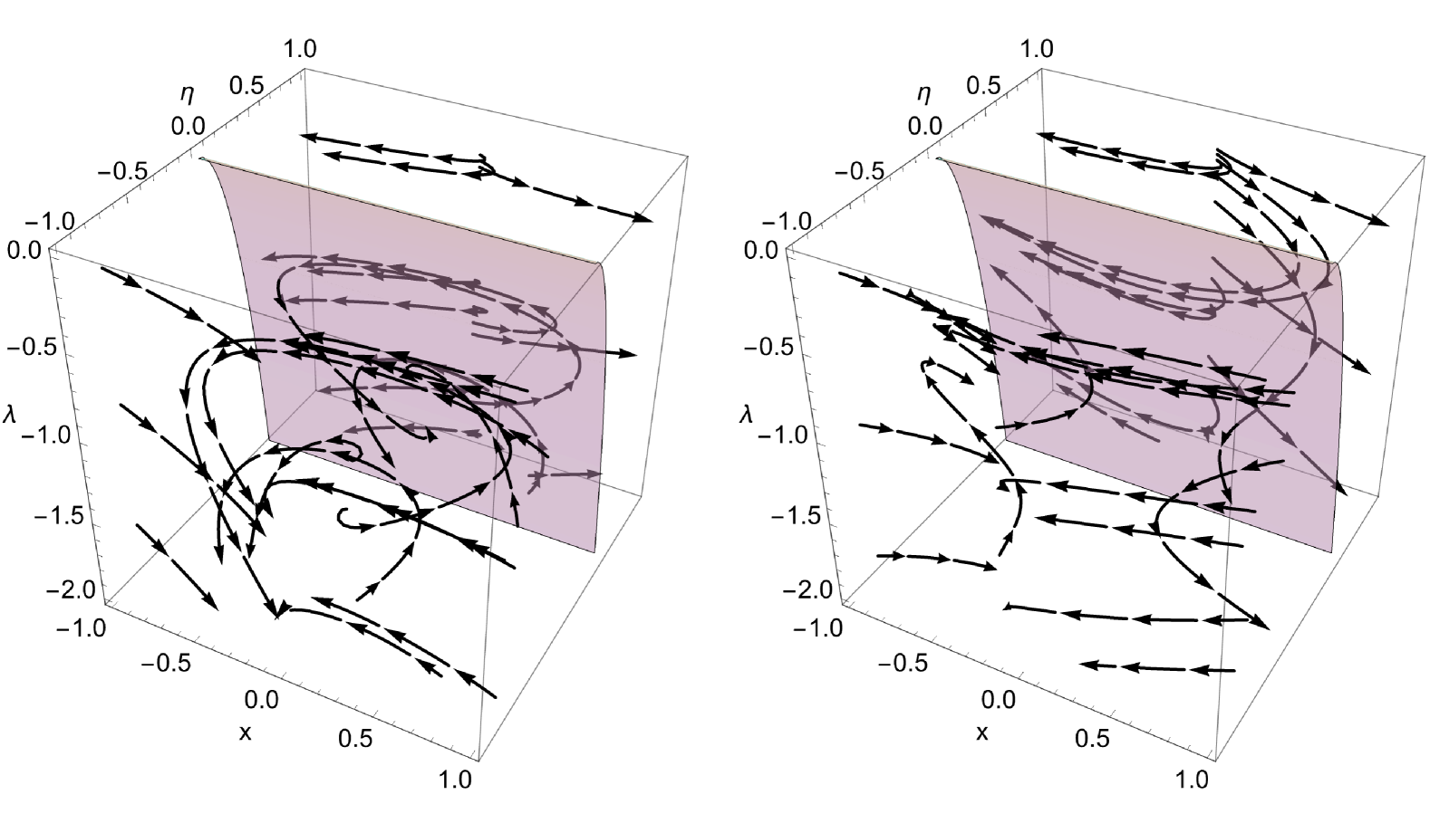
Figure 2: Phase-space portrait for the dynamical system (21), (22) and (24) in the variables $x,\eta~$and $\lambda$ where the family of points $C_{3}$ is marked. Left Fig. is for $n=\frac{1}{5}$ and right Fig. for  $n=-\frac{1}{5}$ . It is easy to see that for $n=\frac{1}{5}$, the trajectories lie on the stable surface $C_{3}$, and the de Sitter solution is an attractor.

VI Final remarks

In this work, we explored a field-equivalent representation of $f(G)$-theories of gravity, with the aim of investigating the phase-space dynamics and the corresponding stability. To do so, we specifically considered a FLRW universe with flat topology and introduced a Lagrange multiplier within the modified Lagrangian density, de facto reformulating the action of $f(G)$-gravity into an equivalent form of Einstein-Gauss-Bonnet scalar field cosmology, that does not exhibit an explicit scalar field kinetic term.

Accordingly, the scalar field potential is directly related to the function $f(G)$ and its derivatives. Further, within this scalar field formulation, we computed the cosmological field equations and introduced a set of dimensionless variables, quite different from those used in standard approach, i.e., carrying out a global dynamical analysis by enabling the Hubble rate to change its sign.

In view of the fact that the field equations constituted a complicated constrained dynamical system, by utilizing the constraint equation, we reduced the system’s dimensionality by one, reducing to four. In addition, we showed that, using an exponential potential, the dynamical system is further reduced by another dimensionality. Afterwards, we identified the equilibrium points and found two attractors, both independent from the spatial curvature.

Within our analysis, one equilibrium point described an expanding, accelerating universe, not behaving as a de Sitter solution, while another one corresponded to a collapsing spacetime.

More precisely, even though a de Sitter solution exists, it manifests as a saddle point. Nevertheless, the phase-space analysis indicated that most initial conditions lead to a collapsed universe, pointing out that our scenario is likely unphysical.

Indeed, in the power-law $f(G)$-theory, the scaling solution appears absent, and the de Sitter solution is not a future attractor for positive values of the power parameter.

Hence, we considered a generic function $\Gamma(\lambda)$ and, then, we employed the equilibrium points of the dynamical system, described by the exponential potential for each root of the algebraic equation $\Gamma(\lambda_{0})-1=0$. Additionally, they corresponded to the points described by the power-law potential with $x=0$ and an arbitrary $\lambda$. We demonstrated that the form of $\Gamma(\lambda)$ determines the number of distinct roots $\lambda_{0}$ and influences the stability properties of the stationary points.

Future works will try to extend our treatment to more physical contexts in which the topological terms may imply more stable regions, whose physical sense can be more defined. In particular, by adding further external fields, such as sources to the energy momentum-tensor or trying to include additional constraints. The impact of perturbations will be also investigated, in order to fix more carefully the free parameters of the theory, as well as possible additional potentials, based on precise physical meanings, related to dark energy sources 2024arXiv241010935C or inflationary domains.

- [1] Edmund J. Copeland, M. Sami, and Shinji Tsujikawa. Dynamics of Dark Energy. International Journal of Modern Physics D, 15(11):1753–1935, January 2006.
- [2] Christine Gruber and Orlando Luongo. Cosmographic analysis of the equation of state of the universe through Padé approximations. Phys. Rev. D, 89(10):103506, 2014.
- [3] Álvaro de la Cruz-Dombriz, Peter K. S. Dunsby, Orlando Luongo, and Lorenzo Reverberi. Model-independent limits and constraints on extended theories of gravity from cosmic reconstruction techniques. JCAP, 12:042, 2016.
- [4] Varun Sahni and Alexei Starobinsky. Reconstructing Dark Energy. Int. J. Mod. Phys. D, 15:2105–2132, 2006.
- [5] Peter K. S. Dunsby, Orlando Luongo, and Lorenzo Reverberi. Dark Energy and Dark Matter from an additional adiabatic fluid. Phys. Rev. D, 94(8):083525, 2016.
- [6] Kazuharu Bamba, Salvatore Capozziello, Shin’ichi Nojiri, and Sergei D. Odintsov. Dark energy cosmology: the equivalent description via different theoretical models and cosmography tests. Astrophys. Space Sci., 342:155–228, 2012.
- [7] Michel Chevallier and David Polarski. Accelerating Universes with Scaling Dark Matter. International Journal of Modern Physics D, 10(2):213–223, January 2001.
- [8] Eric V. Linder. Exploring the Expansion History of the Universe. Phys. Rev. Lett., 90(9):091301, March 2003.
- [9] Joan Simon, Licia Verde, and Raul Jimenez. Constraints on the redshift dependence of the dark energy potential. Phys. Rev. D, 71(12):123001, June 2005.
- [10] Orlando Luongo and Marco Muccino. Kinematic constraints beyond z 0 using calibrated GRB correlations. A&A, 641:A174, September 2020.
- [11] Orlando Luongo and Marco Muccino. Model-independent calibrations of gamma-ray bursts using machine learning. MNRAS, 503(3):4581–4600, May 2021.
- [12] Claus Kiefer. Quantum gravity - an unfinished revolution. 2 2023.
- [13] Jerome Martin. Everything You Always Wanted To Know About The Cosmological Constant Problem (But Were Afraid To Ask). Comptes Rendus Physique, 13:566–665, 2012.
- [14] Orlando Luongo and Marco Muccino. Speeding up the universe using dust with pressure. Phys. Rev. D, 98(10):103520, 2018.
- [15] Alessio Belfiglio, Roberto Giambò, and Orlando Luongo. Alleviating the cosmological constant problem from particle production. Class. Quant. Grav., 40(10):105004, 2023.
- [16] Orlando Luongo and Tommaso Mengoni. Quasi-quintessence inflation with non-minimal coupling to curvature in the Jordan and Einstein frames. 9 2023.
- [17] T. Padmanabhan. Cosmological constant-the weight of the vacuum. Phys. Rep., 380(5-6):235–320, July 2003.
- [18] Sean M. Carroll, William H. Press, and Edwin L. Turner. The cosmological constant. Annual Rev. of Astron. Astrophys., 30:499–542, January 1992.
- [19] Steven Weinberg. The cosmological constant problem. Reviews of modern physics, 61(1):1, 1989.
- [20] Salvatore Capozziello, Anupam Mazumdar, and Giuseppe Meluccio. The Weinberg no-go theorem for cosmological constant and nonlocal gravity. 2 2025.
- [21] Orlando Luongo and Marco Muccino. Model-independent cosmographic constraints from DESI 2024. A&A, 690:A40, October 2024.
- [22] Narayan Khadka, Orlando Luongo, Marco Muccino, and Bharat Ratra. Do gamma-ray burst measurements provide a useful test of cosmological models? JCAP, 09:042, 2021.
- [23] Orlando Luongo, Marco Muccino, Eoin Ó. Colgáin, M. M. Sheikh-Jabbari, and Lu Yin. Larger H0 values in the CMB dipole direction. Phys. Rev. D, 105(10):103510, 2022.
- [24] Peter K. S. Dunsby and Orlando Luongo. On the theory and applications of modern cosmography. Int. J. Geom. Meth. Mod. Phys., 13(03):1630002, 2016.
- [25] Simone Vilardi, Salvatore Capozziello, and Massimo Brescia. Discriminating among cosmological models by data-driven methods. 8 2024.
- [26] Salvatore Capozziello, Peter K. S. Dunsby, and Orlando Luongo. Model-independent reconstruction of cosmological accelerated–decelerated phase. Mon. Not. Roy. Astron. Soc., 509(4):5399–5415, 2021.
- [27] Thomas P. Sotiriou and Valerio Faraoni. f(R) Theories Of Gravity. Rev. Mod. Phys., 82:451–497, 2010.
- [28] Shin’ichi Nojiri and Sergei D. Odintsov. Can F(R)-gravity be a viable model: the universal unification scenario for inflation, dark energy and dark matter. In 17th Workshop on General Relativity and Gravitation in Japan, pages 3–7, 1 2008.
- [29] Shin’ichi Nojiri and Sergei D. Odintsov. Dark energy, inflation and dark matter from modified F(R) gravity. TSPU Bulletin, N8(110):7–19, 2011.
- [30] Alexei A. Starobinsky. A New Type of Isotropic Cosmological Models Without Singularity. Phys. Lett. B, 91:99–102, 1980.
- [31] John D. Barrow and S. Cotsakis. Inflation and the Conformal Structure of Higher Order Gravity Theories. Phys. Lett. B, 214:515–518, 1988.
- [32] John D. Barrow and S. Cotsakis. Selfregenerating inflationary universe in higher order gravity in arbitrary dimension. Phys. Lett. B, 258:299–304, 1991.
- [33] Pablo Bueno, Pablo A. Cano, A. Oscar Lasso, and Pedro F. Ramírez. f(Lovelock) theories of gravity. JHEP, 04:028, 2016.
- [34] D. Lovelock. The Einstein tensor and its generalizations. J. Math. Phys., 12:498–501, 1971.
- [35] S. Nesseris, S. Basilakos, E. N. Saridakis, and L. Perivolaropoulos. Viable models are practically indistinguishable from CDM. Phys. Rev. D, 88:103010, 2013.
- [36] Chao-Qiang Geng, Chung-Chi Lee, Emmanuel N. Saridakis, and Yi-Peng Wu. “Teleparallel” dark energy. Phys. Lett. B, 704:384–387, 2011.
- [37] Andronikos Paliathanasis, John D. Barrow, and P. G. L. Leach. Cosmological Solutions of Gravity. Phys. Rev. D, 94(2):023525, 2016.
- [38] L. K. Duchaniya, Kanika Gandhi, and B. Mishra. Attractor behavior of f(T) modified gravity and the cosmic acceleration. Phys. Dark Univ., 44:101461, 2024.
- [39] Rocco D’Agostino and Orlando Luongo. Growth of matter perturbations in nonminimal teleparallel dark energy. Phys. Rev. D, 98(12):124013, 2018.
- [40] Lavinia Heisenberg. Review on f(Q) gravity. Phys. Rept., 1066:1–78, 2024.
- [41] M. Koussour and Avik De. Observational constraints on two cosmological models of f(Q) theory. Eur. Phys. J. C, 83(5):400, 2023.
- [42] Raja Solanki, Avik De, and P. K. Sahoo. Complete dark energy scenario in f(Q) gravity. Phys. Dark Univ., 36:100996, 2022.
- [43] Fotios K. Anagnostopoulos, Spyros Basilakos, and Emmanuel N. Saridakis. First evidence that non-metricity f(Q) gravity could challenge CDM. Phys. Lett. B, 822:136634, 2021.
- [44] Jose Beltrán Jiménez, Lavinia Heisenberg, and Tomi S. Koivisto. The Geometrical Trinity of Gravity. Universe, 5(7):173, 2019.
- [45] T. Padmanabhan and D. Kothawala. Lanczos-Lovelock models of gravity. Phys. Rept., 531:115–171, 2013.
- [46] Gustavo Dotti, Julio Oliva, and Ricardo Troncoso. Exact solutions for the Einstein-Gauss-Bonnet theory in five dimensions: Black holes, wormholes and spacetime horns. Phys. Rev. D, 76:064038, 2007.
- [47] Christos Charmousis and Jean-Francois Dufaux. General Gauss-Bonnet brane cosmology. Class. Quant. Grav., 19:4671–4682, 2002.
- [48] Ekaterina O. Pozdeeva, Mohammad Sami, Alexey V. Toporensky, and Sergey Yu. Vernov. Stability analysis of de Sitter solutions in models with the Gauss-Bonnet term. Phys. Rev. D, 100(8):083527, 2019.
- [49] Baojiu Li, John D. Barrow, and David F. Mota. The Cosmology of Modified Gauss-Bonnet Gravity. Phys. Rev. D, 76:044027, 2007.
- [50] S. Nojiri, S. D. Odintsov, V. K. Oikonomou, and Arkady A. Popov. Ghost-free gravity. Nucl. Phys. B, 973:115617, 2021.
- [51] Shin’ichi Nojiri and S. D. Odintsov. Black holes, photon sphere, and cosmology in ghost-free f(G) gravity. Phys. Dark Univ., 46:101702, 2024.
- [52] N. Myrzakulov, Anirudh Pradhan, Archana Dixit, and S. H. Shekh. Exploring Phase Space Trajectories in CDM Cosmology with f(G) Gravity Modifications. 9 2024.
- [53] Santosh V. Lohakare, Soumyadip Niyogi, and B. Mishra. Cosmology in modified gravity: a late time cosmic phenomena. Mon. Not. Roy. Astron. Soc., 535:1136, 2024.
- [54] Kazuharu Bamba, M. Ilyas, M. Z. Bhatti, and Z. Yousaf. Energy Conditions in Modified Gravity. Gen. Rel. Grav., 49(8):112, 2017.
- [55] I. V. Fomin. Cosmological Inflation with Einstein–Gauss–Bonnet Gravity. Phys. Part. Nucl., 49(4):525–529, 2018.
- [56] S. D. Odintsov, V. K. Oikonomou, and F. P. Fronimos. Non-minimally coupled Einstein–Gauss–Bonnet inflation phenomenology in view of GW170817. Annals Phys., 420:168250, 2020.
- [57] Andronikos Paliathanasis. 4D Einstein–Gauss–Bonnet cosmology with Chameleon mechanism. Gen. Rel. Grav., 56(7):84, 2024.
- [58] Alfredo D. Millano, Claudio Michea, Genly Leon, and Andronikos Paliathanasis. Dynamics of a higher-dimensional Einstein–Scalar–Gauss–Bonnet cosmology. Phys. Dark Univ., 46:101589, 2024.
- [59] José Jaime Terente Díaz, Konstantinos Dimopoulos, Mindaugas Karčiauskas, and Antonio Racioppi. Gauss-Bonnet Dark Energy and the speed of gravitational waves. JCAP, 10:031, 2023.
- [60] Shin’ichi Nojiri and Sergei. D. Odintsov. Propagation speed of gravitational wave in scalar–Einstein–Gauss-Bonnet gravity. Nucl. Phys. B, 998:116423, 2024.
- [61] Saddam Hussain, Simran Arora, Yamuna Rana, Benjamin Rose, and Anzhong Wang. Interacting models of dark energy and dark matter in Einstein scalar Gauss Bonnet gravity. JCAP, 11:042, 2024.
- [62] Edmund J. Copeland, M. Sami, and Shinji Tsujikawa. Dynamics of dark energy. Int. J. Mod. Phys. D, 15:1753–1936, 2006.
- [63] Peter K. S. Dunsby and Orlando Luongo. On the theory and applications of modern cosmography. International Journal of Geometric Methods in Modern Physics, 13(3):1630002–606, January 2016.
- [64] Alejandro Aviles, Christine Gruber, Orlando Luongo, and Hernando Quevedo. Cosmography and constraints on the equation of state of the Universe in various parametrizations. Phys. Rev. D, 86(12):123516, December 2012.
- [65] Alejandro Aviles, Alessandro Bravetti, Salvatore Capozziello, and Orlando Luongo. Precision cosmology with Padé rational approximations: Theoretical predictions versus observational limits. Phys. Rev. D, 90(4):043531, August 2014.
- [66] Alejandro Aviles, Jaime Klapp, and Orlando Luongo. Toward unbiased estimations of the statefinder parameters. Physics of the Dark Universe, 17:25–37, September 2017.
- [67] Youri Carloni and Orlando Luongo. Phase-space analysis in non-minimal symmetric-teleparallel dark energy. Eur. Phys. J. C, 84(5):519, 2024.
- [68] Youri Carloni and Orlando Luongo. Stability of non-minimally coupled dark energy in the geometrical trinity of gravity. arXiv e-prints, page arXiv:2410.10935, October 2024.
- [69] Ruth Lazkoz, Genly Leon, and Israel Quiros. Quintom cosmologies with arbitrary potentials. Phys. Lett. B, 649:103–110, 2007.
- [70] Andronikos Paliathanasis, Amlan Halder, and Genly Leon. Revise the Dark Matter-Phantom Scalar Field Interaction. arXiv e-prints, 2412.06501, 2024.
- [71] G. Papagiannopoulos, John D. Barrow, S. Basilakos, A. Giacomini, and A. Paliathanasis. Dynamical symmetries in Brans-Dicke cosmology. Phys. Rev. D, 95(2):024021, 2017.