Bayesian optimization of beam injection and storage in the PSI muEDM Experiment

Abstract

The muEDM experiment at the Paul Scherrer Institute aims to measure the electric dipole moment with an unprecedented sensitivity of $6\times 10^{-23}\,\mathrm{e}\cdot\mathrm{cm}$. A key aspect of this experiment is the injection and storage of the muon beam, which traverses a long, narrow superconducting channel before entering a solenoid magnet. The muon is then kicked by a pulsed magnetic field into a stable orbit within the solenoid’s central region, where the electric dipole moment is measured. To study the beam injection and storage process, we developed a G4beamline simulation to model the dynamics of beam injection and storage, incorporating all relevant electric and magnetic fields. We subsequently employed a Bayesian optimization technique to improve the muon storage efficiency for Phase I of the muEDM experiment. The optimization is demonstrated using data simulated by G4beamline. We have observed an enhancement in the beam injection and storage efficiency, which increased to 0.556% through the utilization of Bayesian optimization with Gaussian processes, compared to 0.324% when employing the polynomial chaos expansion. This approach can be applied to adjust actual experimental parameters, aiding in achieving the desired performance for beam injection and storage in the muEDM experiment.

I Introduction

In accelerator and storage ring experiments, beam injection and storage in both simulations and real-world experiments demand significant computational and time resources, making the optimization landscape complex and often non-linear with multiple interacting parameters. This complexity is exacerbated by the presence of operational noise and the resource-intensive nature of beam physics simulations. In precision muon physics experiments, such as the Muon $g-2$ experiment Muong-2:2023cdq ; Muong-2:2024hpx at Fermilab and the muEDM experiment Adelmann:2025nev ; Adelmann:2021udj at Paul Scherrer Institute (PSI), beam injection and storage play a critical role because of the need for high muon decay statistics of these studies. In the Fermilab and PSI experiment, the challenge arises from the mismatch between the beam’s phase space and the storage ring’s or solenoid’s acceptance phase space, compounded by the very narrow superconducting beam injection channel Kim:2017jfd ; Froemming:2019gcn ; muEDM:2024bri . As a result, achieving optimal beam storage efficiency has proven to be a daunting task in these experiments.

Recently, Bayesian Optimization (BO) 7352306 has emerged as a valuable algorithm within the accelerator community. It offers effective solutions for addressing complex optimization challenges under noise and resource constraints during accelerator operation and resource-intensive beam physics simulations Roussel:2023yin . This algorithm employs probabilistic surrogate models along with an acquisition function to balance exploration and exploitation, minimizing the number of evaluations. BO has been successfully applied in storage ring facilities, such as the Karlsruhe Research Accelerator (KARA) Xu:2022ygq and the Synchrotron Light Source DELTA at TU Dortmund University Schirmer:2023vdn . The Cooler Synchrotron storage ring COSY at Forschungszentrum Julich used BO for the optimization of the Injection Beam Line (IBL) to increase the beam intensity inside the storage ring Awal:2023lpt . With the advent of Laser Plasma Accelerators (LPAs), BO has been successfully demonstrated in simulations for concurrently optimizing the localized properties of compact free electron lasers (FELs) driven by laser wakefield accelerators (LWFAs), maximizing energy extraction efficiency and ensuring high-quality electron beams with reduced energy spread and emittance Zhong:2024 ; Jiang:2025 . Additionally, BO has found applications in other domains, such as maximizing the Linac Coherent Light Source (LCLS) x-ray free-electron laser (FEL) pulse energy by controlling groups of quadrupole magnets Duris:2019xwc and optimizing multiple objectives in the MeV-ultrafast electron diffraction experiment at SLAC Ji:2024gfq .

In this paper, we explore the use of BO to maximize storage efficiency in the Muon Electric Dipole Moment (muEDM) experiment at the Paul Scherrer Institute (PSI), focusing on optimizing the beam injection and storage within the storage solenoid of the experiment. The muEDM experiment at PSI aims to search for the muon electric dipole moment (EDM) with an unprecedented sensitivity of $6\times 10^{-23}e\cdot$cm, which is 4 orders of magnitude better than the current limit Muong-2:2008ebm . Detecting a muon EDM larger than the Standard Model (SM) predictions Cabibbo:1963yz ; Kobayashi:1973fv ; Pospelov:2013sca ; Yamaguchi:2020eub would provide an unambiguous hint of physics beyond the SM. Since the EDM violates time-reversal (T) symmetry, it also violates Charge-Parity (CP) symmetry, given that CPT symmetry is conserved. Therefore, the EDM can reveal new sources of CP violation, potentially shedding light on the matter-antimatter asymmetry observed in our universe Sakharov:1967dj ; WMAP:2010qai .

The muEDM experiment consists of two phases: Phase I and Phase II. Phase-I serves as a precursor experiment for the frozen-spin technique, aiming for a sensitivity goal of $3\times 10^{-21}e\cdot$cm. In Phase-I of the muEDM experiment PSImuEDM:2023dsd , the 28 MeV/c surface muon beam at the $\pi$E1 beamline of PSI will be injected into the PSC solenoid with an inner diameter of 0.2 m and a length of 1 m, through a collimation tube with superconducting shield muEDM:2023mtc that are 15 mm in diameter and 800 mm long. The tube selects the appropriate phase space and shields the solenoid’s fringe magnetic field. Inside the solenoid, five other coils generate a magnetic field to store the muons in the central region; these include a pair of correction coils, a weakly focusing coil, and a pulse coil muEDM:2024bri . When the muons exit the collimation tube and enter the 3-T magnetic field, they pass through a muon trigger detector Hu:2024avd ; Wong:2024wol ; Hu:2025tgk , generating a signal that triggers the pulsed magnetic field, converting the longitudinal momentum of the muons into transverse momentum, which allows the muons to be stored in the weakly focused field. This beam injection scheme is motivated by the 3D spiral beam injection strategy Matsushita:2023zho of the J-PARC Muon $g-2$/EDM experiment Abe:2019thb . During storage, muons will circulate at a radius of $r=31$ mm with a cyclotron period of about 2.5 ns until the muon decays into positrons and muon neutrinos. A radial electric field of 3 kV/cm is applied by concentric cylindrical electrodes surrounding the muon orbit at $r=40$ mm (ground) and $r=20$ mm (high voltage) to satisfy the frozen-spin condition for measuring the muon EDM muEDM:2024bri . A schematic view of the experiment is shown in Fig. 1.

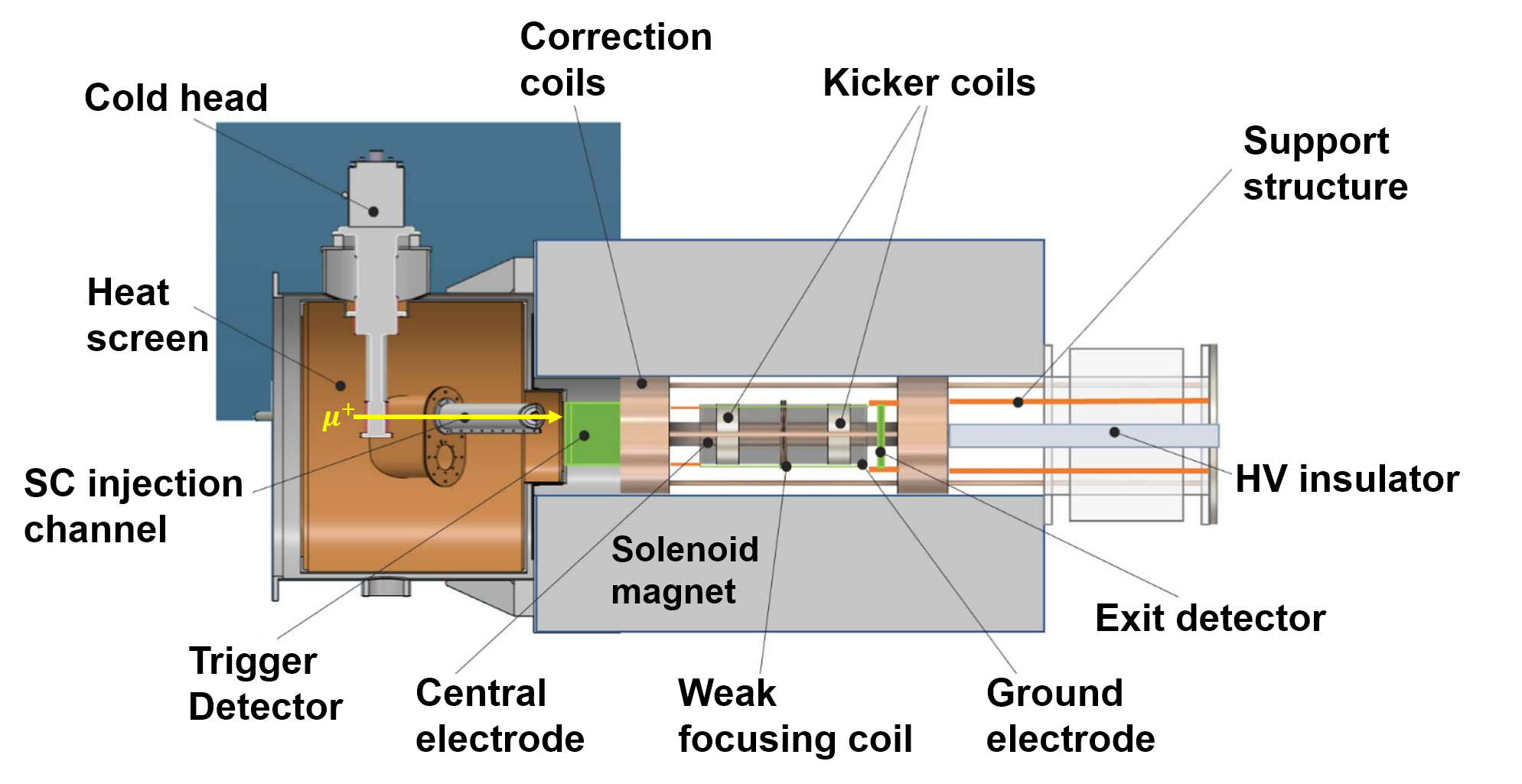
Figure 1: A schematic view of the muEDM experiment at PSI for Phase-I. It encompasses all components integral to the study presented herein, including the superconducting injection channel, the central electrode, kicker coils, and the weak focusing coil.

This paper is organized as follows: In Sec. II, we provide an overview of the beam injection and storage process in the muEDM experiment, along with details about the simulation toolkit used in the optimization process. Section III presents optimization studies focused on identifying a set of injection parameters that optimize the number of stored muons, including a comprehensive analysis of the BO technique. In Sec. IV, the results are discussed, and the implications of our findings are elaborated upon. Finally, this paper is summarized in Sec. V.

II Beam Injection and Storage Simulation

II.1 Beam Injection Phase Space at PSI’s $\pi$E1 Beamline

The $\pi$E1 beamline at PSI provides high-intensity pion and muon beams with momenta ranging from 10 MeV/c to 500 MeV/c and a momentum resolution better than 0.8%. The beam is extracted from a carbon target, passes through dipoles and a Wien filter to select a muon beam with low contamination, and is tuned for the desired spin orientation. Beam transport to the experimental area is accomplished using quadrupole triplets for focusing and steering. Based on the measured transverse phase space of the $\pi$E1 beam Papa:2015lda , the transmission efficiency is manually optimized through simulation using injection tubes with different diameters $d_{\rm{inj}}$, indicating that $d_{\rm{inj}}$ = 15 mm with a length of 800 mm strikes a good balance in the selection and transmission of phase space. The beam profile after passing through the injection tube is shown in Fig. 2.

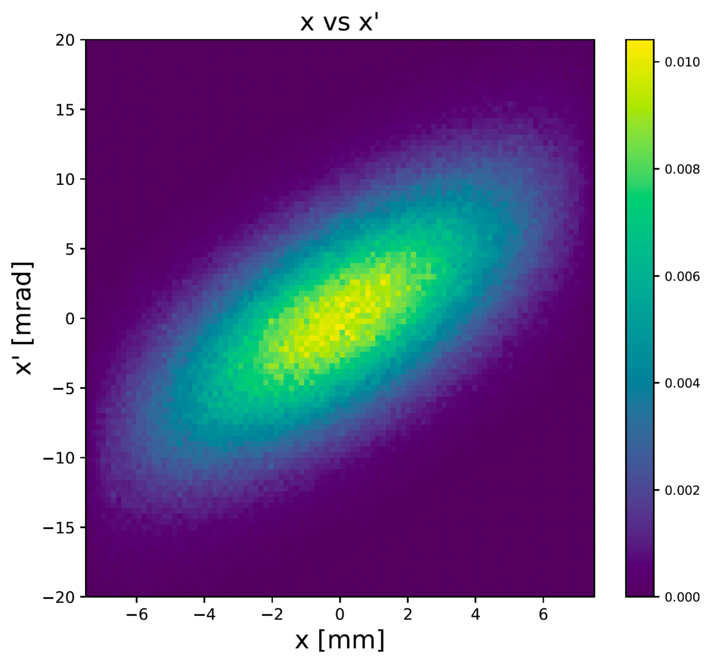
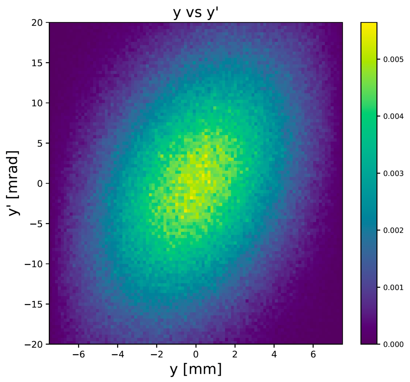
Figure 2: Monte-Carlo generated $x$ (Top) and $y$ (Bottom) phase space after transmission through the injection tube with the total transmission of 3%, with $x$ and $y$ emittance of 14.8 mrad, and 32.0 mrad respectively.

II.2 Simulation Framework and Modeling Tools

The simulated phase space at the end of the injection tube, as depicted in Fig. 2, was utilized to generate $5\times 10^{6}\,\mu^{+}/s$ events for the subsequent simulation phase. G4Beamline Roberts:2007nte serves as a platform for prototyping the beam injection simulation, wherein the muon is introduced via an off-axis injection scheme into the PSC solenoid bore, which possesses dimensions of $x=200$ mm in diameter and $z=1000$ mm in length. The employed 3-T magnetic field is modeled by fitting empirical data to a calculated field, followed by the adjustment of both solenoid coil and split coil pair parameters within an ANSYS simulation Alawadhi:2015 .

A pair of correction coils, with inner and outer radii measuring 90 mm and 99.9 mm respectively, along with a length of 90 mm, is powered by a current of 2.5 A/mm². These coils are simulated at position $z=\pm 250$ mm to enhance the acceptance of the injection phase space between the exit of the injection tube and the storage range. Additionally, a magnetic coil with inner and outer radii of 50 mm and 60 mm, and a length of 10 mm, is positioned 100 mm apart with anti-parallel currents. This coil is simulated at the center to create the pulsed magnetic kicker field. The configuration of the magnetic pulsed kicker, as depicted in Fig. 3, is modeled based on a simulation derived from the circuit design tool LTspice .

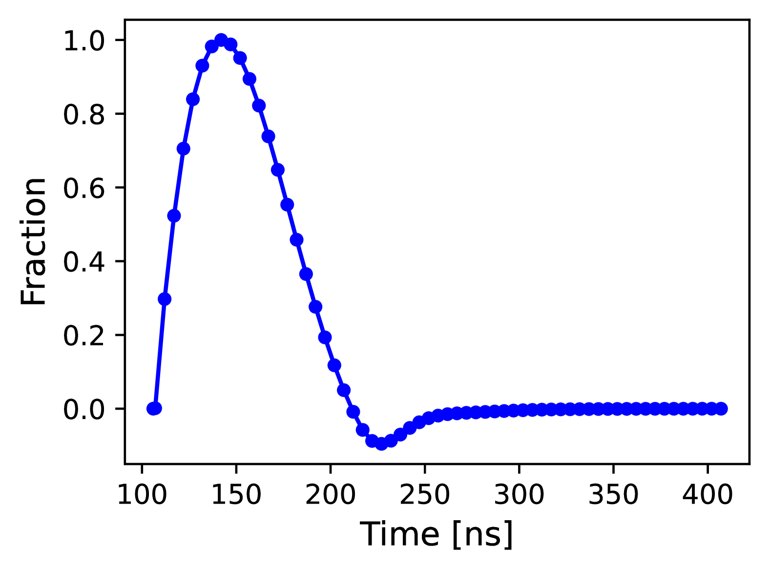
Figure 3: Kicker pulse current profiles simulated using the LTspice circuit model. The simulated time range is from $t=0$ to $t=500$ ns, whereas $t=0$ signifies the beam entrance into the storage solenoid.

The weakly focusing coil, with an inner radius of 50 mm, an outer radius of 60 mm, and a length of 10 mm, is simulated at the center to provide longitudinal confinement for the muon with a current of 1.5 A/mm². The coaxial electrodes, which are 120 mm long and made of carbon and copper, consist of a high-voltage (HV) electrode and a ground electrode. These electrodes are used to create the electric field necessary for maintaining the frozen spin condition. The magnetic fields generated by both the correction coil and the weakly focusing coil are modeled using G4Beamline, while the electric field is modeled using ANSYS.

The simulation models the muon injection process into a storage region, taking into account various injection parameters that influence beam dynamics and efficiency. The injection geometry is defined by the injection angle, $\theta$, and transverse angle, $\phi$, both measured in degrees, which determine the muon’s entry trajectory. The injection angle, $\theta$, is the angle formed by the injection tube with respect to the Z-axis, while the transverse angle, $\phi$, is the angle measured relative to the Y-axis, located at the rear side of the PSC solenoid. The injection radius, $R_{\rm{inj}}$, and the longitudinal injection coordinate, $Z$, both measured in millimeters, specify the spatial entry point. The injection radius, $R_{\rm{inj}}$, is the radial distance from the rear center to the desired injection circumference. Furthermore, the weakly-focusing coil current, $A_{\text{weak}}$, expressed in Amperes per millimeter (A/mm), is vital for shaping the field to confine the muon beam. The kicker field strength, BPI, and the pulsed kicker time offset (KPT), measured in nanoseconds (ns), is relative to the shape of the kicker pulse Fig. 3, regulate beam steering and timing, ensuring optimal injection and subsequent storage conditions. Collectively, these beam injection and storage parameters are summarized in Tab. 1.

Table 1: The list of parameters used in the baseline simulation optimization study.

Parameter symbol	Description
$R_{\rm{inj}}$	Injection radius (mm)
Z	Longitudinal injection coordinate (mm)
$\theta$	Injection angle (degree)
$\phi$	Transverse angle (degrees)
$A_{weak}\times 100$	Weak current $\times$ 100 (A/mm)
BPI	Strength of pulsed kicker (arb. units)
KPT	Time offset of pulsed kicker (ns)

For a specified set of injection parameter inputs, the stored muon efficiency, $\epsilon$, is given by the equation:

$$\epsilon=\frac{N_{\rm{stored}}}{N_{\rm{injected}}}$$ (1)

where the $N_{\rm{stored}}$ is the number of stored muons retained in the central region given by $|z|<40\,\text{mm}$. On top of that, these muons shall remain in this region for a duration more than 300 ns, given that the total elapsed time from their exit from the injection tube to their arrival in the central region is approximately 200 ns. Additionally, $N_{\rm{injected}}$ represents the total number of muons that have been injected. In other words, the number of muons passed through the injection tube. A typical stored muon event, as simulated within the G4beamline framework, is illustrated in Fig. 4.

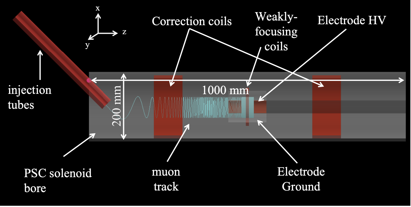
Figure 4: Visualization of a beam injection and storage event into the PSC magnet in the G4Beamline simulation. The image depicts a “pencil” muon beam trajectory inside the solenoid bore. Key components are labeled, including the injection tube, correction coils, weakly focusing coils, and high-voltage electrodes, which play crucial roles in guiding and storing the muon beam within the 1000 mm-long solenoid.

III Optimization Methodology

III.1 Initial Optimization with Polynomial Chaos Expansion

Since the BO routine is very sensitive to the initial parameter choices and bounds, we first employed a surrogate model based on Polynomial Chaos Expansion (PCE) to expedite our process before utilizing BO for optimal beam injection and storage parameters computation.

PCE is a spectral expansion method that expresses the response of a system as a series of orthogonal polynomials of input parameters, providing an efficient surrogate modeling approach for complex physical systems. It has been widely used in uncertainty quantification and parametric sensitivity analysis, serving as an alternative to direct numerical simulations, which can be computationally expensive. The surrogate model PCE encodes the responses to a set of input variables, where their distributions are related through an expansion coefficient. This coefficient is calculated using non-intrusive methods, estimated by regression techniques based on the difference between the output predicted by the model and the true response provided by the simulation results. The regression-based estimation of coefficients depends on the number of samples and the integration points.

An 8-dimensional PCE model muEDM:2023xkb based on the injection parameters from Tab. 1 incorporating the kicker width as an additional variable. Additionally, for this iteration, an initial distribution of $10^{6}$ muons was used. Assuming a binomial distribution for successful injection, this would translate to a variance of $\approx 2.0$% for an injection efficiency of $\approx 0.3$%. Thus, the accuracy in this case was limited by both the small number of training samples and the number of muons in the initial distribution used for injection. A 3rd or 4th-degree polynomial expansion was trained using 1,600 samples generated from G4Beamline simulations. The mean squared error (MSE) for the 3rd- or 4th-degree PCE model was in the range of 10^-6 to 10^-7, for the number of training samples. Utilizing the ChaosPy Python toolbox Jonathan:2015 , the generated PCE expansion is then fitted with the trained samples using the least squares regression method muEDM:2023xkb . The optimal value of storage efficiency, as determined, is 0.324%. Although this approach has the potential for further enhancement through the inclusion of additional samples in the training phase—specifically, exceeding 3,000 samples for the fourth-degree polynomial and over 5,000 for the sixth-order polynomial—we have opted to conclude our efforts at this juncture. This decision is predicated on the consideration that further expansion would incur excessive computational costs, whereas our primary objective was to identify reasonable initial parameters and their respective boundaries for the BO routine.

III.2 Bayesian optimization with Gaussian process

Bayesian Optimization is a robust optimization methodology particularly suited for situations where evaluating the objective function is computationally expensive, noisy, or demands considerable time Brochu:2010lgg . This method acts as a global optimization strategy that leverages a probabilistic model to efficiently search for the optimal solution. The iterative nature of BO is key to its efficiency and effectiveness in optimizing complex systems. At each iteration, BO evaluates the objective function at a chosen point in the parameter space, utilizing the surrogate model to anticipate the function’s behavior. This evaluation yields valuable insights into the landscape of the objective function, which then informs updates to the surrogate model. Based on this updated model, an acquisition function is used to select the next sampling point, balancing exploration of uncertain regions and exploitation of areas likely to produce high values. This cycle continues iteratively, with each new evaluation enhancing the model and improving the search for optimal solutions. The BO algorithm utilized in this paper largely follows the pseudocode outlined in Algo. 1 Brochu:2010lgg .

Data: $t\geq 0$

Result: $D_{t}=[X,Y]_{t}$

$Y\leftarrow f_{obj}(\bf{x_{n}})$;

$\bf{X}\leftarrow\bf{x_{0}}$;

$N\leftarrow 1$;

while $N<t$ do

    $\bf{X}\leftarrow\text{argmax }\alpha(\bf{x_{t-1}}|D_{t-1})$;

    ;

     /*Acquisition function*/

    $Y\leftarrow f_{obj}(\bf{X})$;

    $N\leftarrow N+1$;

   

end while

Algorithm 1 Bayesian optimization algorithm

BO consists of two key components: the construction of a surrogate model, typically a Gaussian process (GP), which is commonly employed, and the use of an acquisition function to guide the search for the next evaluation point Rasmussen:2005 ; Xu:2022ygq . A GP is a non-parametric statistical model that provides a distribution over possible objective functions, a belief that those objective functions are drawn from some prior probability distribution $p(A)$. After an observation is made, the posterior distribution $p(A|f(x))$ is constructed based on the Bayes’ theorem:

$$p(A|f(x))\propto p(f(x)|A)p(A)$$ (2)

The posterior distribution is further used to build an acquisition function, which determines the next point for evaluation. The general GP function for a given input variable, $\bf{x}$ is given by:

$$f(x)\sim\mathcal{GP}(\mu(\bf{x}),k(\bf{x},\bf{x}^{\prime}))$$ (3)

consists of mean function $\mu(\bf{x})$, represents the best estimate of the objective function at a given point based on previous evaluations, and covariance function or kernel function $k(\bf{x},\bf{x}^{\prime})$, encodes our assumptions, $\bf{x}^{\prime}$ about the smoothness and correlation of the objective function, helping to predict where the function is likely to have optimal values. The BO uses the Radial Basis Function (RBF) kernel commonly employed for its smoothness properties MAJDISOVA2017728 :

$$k_{RBF}(\textbf{x},\textbf{x'})=exp\left[-\frac{1}{2}\sum_{i=1}^{d}(\frac{\textbf{x}_{i}-\textbf{x}^{\prime}_{j}}{\ell_{i}})^{2}\right]$$ (4)

in which $l_{i}$ is the length scale for each dimension ($i$th), and $d$ is the dimensionality of the input space. This kernel ensures a smooth interpolation of the objective function and incorporates the effects of scale and variability in the data. The stochastic noise present in the system is emulated by explicitly adding Gaussian distributed noise $\sigma_{noise}$ to the covariance function as diagonal terms. Thus, the kernel function becomes:

$$k(\bf{x},\bf{x}^{\prime})=\sigma^{2}k_{RBF}(\textbf{x},\textbf{x'})+\sigma^{2}_{\text{noise}}\delta_{ij}$$ (5)

The signal variance $\sigma^{2}$, noise $\sigma_{noise}$, and the length scale $\ell$ represent the hyperparameters for the BO model, which determine the behavior of the GP.

BO employs an acquisition function to determine the next evaluation point in the parameter space. The acquisition function is designed to balance exploration, searching areas with high uncertainty, and exploitation, focusing on areas where the function is likely to be optimal. One of the most common acquisition functions is the Upper Confidence Bound (UCB) method,

$$\alpha_{UCB}=\mu(x)+\kappa\sigma(x)$$ (6)

where $\mu(x)$ is the predicted mean and $\sigma(x)$ is the predictive uncertainty of the GP function. High $\kappa$ values emphasize the uncertainty term, promoting exploration; conversely, small $\sigma(x)$ values reduce the impact of $\sigma(x)$, favoring exploitation by sampling near regions with higher posterior mean values given by the observed peaks. This adaptive strategy enables BO to efficiently navigate complex, high-dimensional parameter spaces with minimal evaluations. The $\kappa$ can also increase along with the evaluation steps to ensure that BO converges to the global optimum Brochu:2010lgg ; 6138914 .

IV Optimization Results

Prior to the optimization of BO, it is essential to establish an initial dataset that accurately represents the injection parameters as detailed in Table 1. This is accomplished by identifying a baseline point at which the corresponding storage efficiency is greater than zero. A parameter scan is then performed within estimated parameter ranges while keeping the remaining six parameters fixed at their baseline values. The optimized range of each parameter is defined as the region where the storage efficiency exceeds 60% of the maximum efficiency. An example of a one-dimensional parameter scan is shown in Fig. 5.

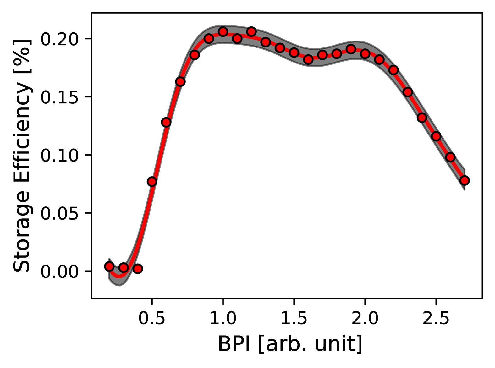
Figure 5: Example of parameter scan for strength of pulse kicker field (BPI), with all other injection parameters kept constant during the scan. The GP hyperparameter ${\ell,\sigma^{2},\sigma_{noise}^{2}}$ are fitted to the scanned points via a log marginal likelihood fit. The solid line red line depicts the GP posterior mean and the shaded region shows the 95% confidence level.

Following this, a total of ten sample points are generated from the seven-dimensional joint parameter space within their respective optimized ranges using the Sobol Sequence SOBOL196786 . Sobol sequences are low-discrepancy sequences known for their superior convergence rates, particularly in lower-dimensional distributions Cheng:2013 . Monte Carlo techniques commonly used to simulate the injection process rely on generating random distributions of input parameters that influence injection and storage efficiency. However, approximations based on Monte Carlo methods inherently have probabilistic error bounds. In contrast, low-discrepancy sequences such as Sobol points provide a deterministic set of sample points that ensure faster convergence and greater accuracy compared to purely random sampling.

Each of these generated sample points is then evaluated using the objective function, with their respective storage efficiencies computed through simulation. These sample points collectively form the initial dataset, denoted as $D_{0}$, providing prior information for the initialization of the BO process.

In the context of the Gaussian Process (GP) function, it is posited that the mean function, represented as $\mu(\mathbf{x})=0$, constitutes a standard selection in situations in which the objective function is not predetermined Xu:2022ygq . The hyperparameters are obtained through one-dimensional parameter scans by fitting GP functions, as detailed in Eq. 5, to the scanned parameter distributions by employing the log marginal likelihood method, as illustrated in Fig. 5. The hyperparameters that correspond to each injection parameter are encapsulated in Tab. 2.

Table 2: Hyperparameters length scale ($\ell$), signal variance ($\sigma^{2}$), and noise ($\sigma_{noise}$), extracted for each parameter.

Parameter	$\ell$	$\sigma^{2}$	$\sigma_{noise}$
$R_{\rm{inj}}$ (mm)	11.3	$0.177$	2.6e-4
Z (mm)	8.22	$0.126$	5.41e-5
$\theta$ (degree)	2.36	$0.123$	1.28e-4
$\phi$ (degree)	12.1	$0.155$	1.79e-4
$A_{weak}\times 100$ ($\rm{A/mm^{2}}$)	50.2	$0.156$	6.89e-6
BPI (arb. unit)	0.38	$0.127$	4.12e-5
KPT (ns)	6.58	$0.112$	2.3e-5

Among the seven injection parameters, the BPI exhibited the smallest length scale in the GP model, indicating that storage efficiency is highly sensitive to variations in BPI. This aligns with expectations, as the BPI directly corresponds to the strength of the pulsed kicker employed to trap muons in the central region of the solenoid. In contrast, geometric parameters such as $R_{\rm{inj}}$ and $\phi$ have larger length scales, suggesting a reduced sensitivity to minor changes in their values. The signal variances for all parameters are relatively similar, implying comparable levels of functional variation among them. The noise levels remain low across all parameters, consistent with well-controlled experimental or simulation conditions setup.

To balance exploration and exploitation during optimization, the acquisition function used a confidence parameter of $\kappa=2$, which corresponds to the 95% confidence interval for Gaussian distributions Xu:2022ygq . For implementing the BO algorithm, the GPy software package gpy2014 was utilized to construct the GP model, while the SciPy Virtanen:2019joe library was employed to maximize the acquisition function. The BO process was performed using 100,000 injection events per iteration and ran for 50 iterations, taking approximately 120 hours to complete. Note that most of the time was spent on running the simulation. The optimization results, along with the parameter evolution across iterations, are shown in Fig. 6. Most parameters exhibit fluctuations early in the optimization process, reflecting exploration during the Bayesian Optimization. As the iterations progress, several parameters, namely $\theta$, $R_{\rm{inj}}$, and $A_{\rm{weak}}$ tend to stabilize, while the others continue to vary, suggesting ongoing exploration of their effects on storage efficiency. The increase in storage efficiency throughout the iterations confirms the optimization process’s success in achieving its goal. A comparison between the optimized results obtained using the PCE method and those from BO is presented in Tab. 3. The BO optimization improved the storage efficiency nearly twofold, from 0.324% (PCE) to 0.556%. The results were cross-validated using the musrSim simulation package Sedlak:2012 , confirming the consistency of the optimized parameter set and the corresponding storage efficiency.

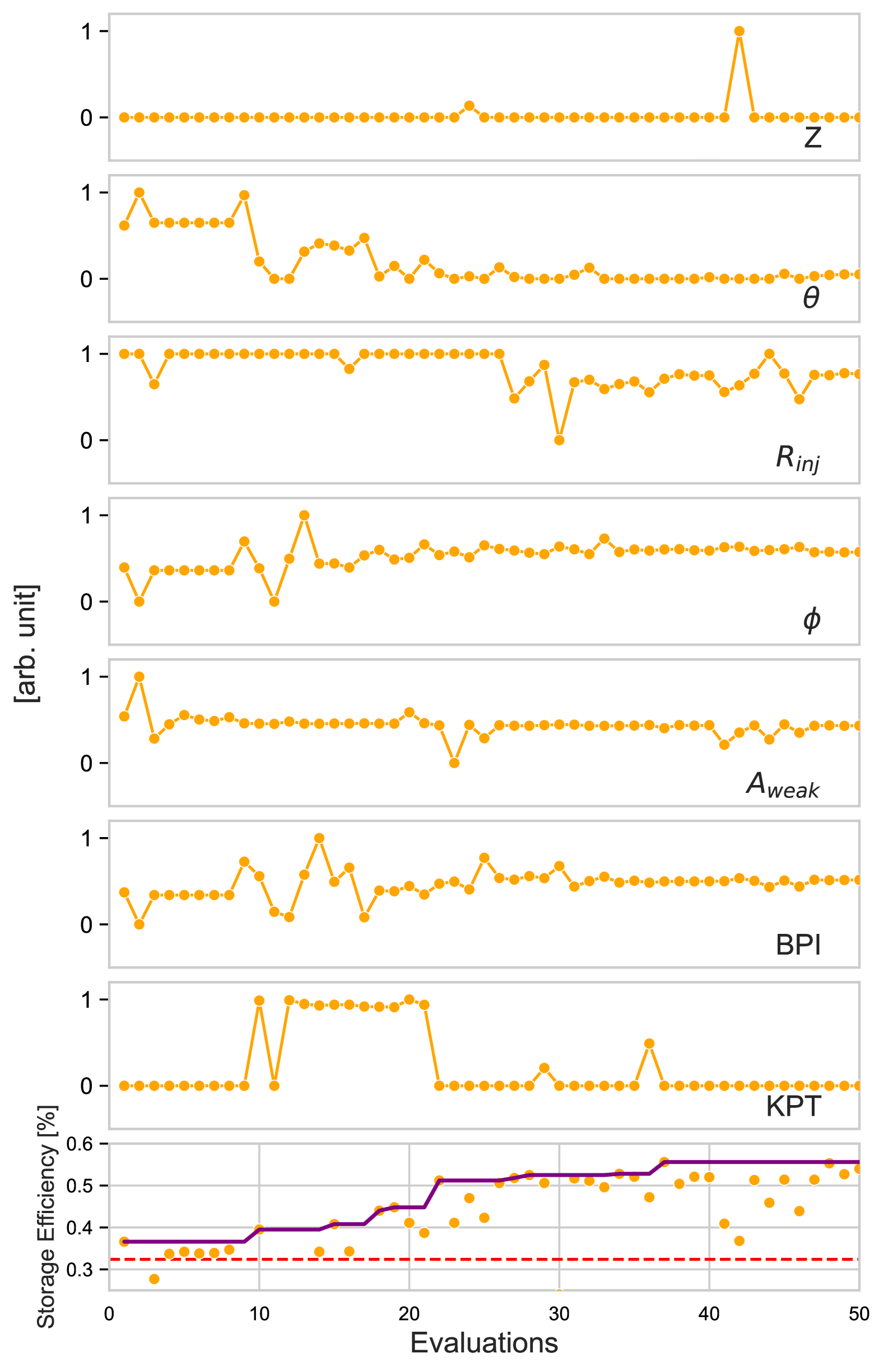
Figure 6: The evolution of the input parameters and the resulting objective function is illustrated across the optimization steps, with the vertical limit representing the total allowed optimization range. The bottom plot displays the muon storage efficiency (orange markers) alongside the cumulative best results (purple line). The red dotted line indicates the muon storage efficiency obtained from the PCE optimization algorithm.

Table 3: Optimized values for the PCE and BO method

Parameter	PCE	BO
$R_{\rm{inj}}$ (mm)	45.56	47.00
Z (mm)	-443.84	-443.69
$\theta$ (degree)	-45.02	-45.00
$\phi$ (degree)	9.24	10.00
$A_{\rm{weak}}\times 100(\rm{A/mm^{2}})$	150.00	202.90
BPI (arb. unit)	1.00	1.50
KPT (ns)	0	-28
Storage efficiency (%)	0.324	0.556

This improvement, however, comes with specific trade-offs. The increase in current for the weakly focusing coil enhances the beam-focusing capabilities, but it also results in higher energy consumption. The increase in kicker field strength improves the stopping of the muons into the storage region, placing additional demands on the kicker system, including greater power requirements and potential wear over extended operational periods. On the other hand, the -28 ns time offset for the pulsed kicker effectively advances the timing of the kicker activation. This earlier activation helps better synchronize the kicker’s operation with the beam injection process, thereby enhancing the efficiency of muon capture. While this adjustment optimizes timing, it may require more precise control and synchronization of the system to maintain consistent performance under varying conditions.

V Summary and Outlook

This study demonstrates the use of Bayesian Optimization to improve beam injection and storage efficiency for the muEDM experiment at the Paul Scherrer Institute (PSI), focused on searching for the muon electric dipole moment. By optimizing a set of defined injection parameters through simulations, the BO framework successfully enhances storage efficiency while minimizing the number of evaluations conducted. This work demonstrates the feasibility of the method and lays the foundation for optimizing beam injection and storage in both Phase I and Phase II of the muEDM experiment, with the current implementation serving as a baseline framework for future development. While the present BO approach may place higher demands on the operational systems of the experiment, incorporating physical safety constraints can limit exploration to safe parameter regions, thereby addressing these challenges. Additionally, extending the single-objective BO framework to a multi-objective optimization approach would enable simultaneous trade-offs between various experimental goals, such as balancing storage efficiency with correction coil geometry and current.

References

- (1) D. P. Aguillard et al. [Muon g-2], “Measurement of the Positive Muon Anomalous Magnetic Moment to 0.20 ppm,” Phys. Rev. Lett. 131, no.16, 161802 (2023) doi:10.1103/PhysRevLett.131.161802 [arXiv:2308.06230 [hep-ex]].
- (2) D. P. Aguillard et al. [Muon g-2], “Detailed report on the measurement of the positive muon anomalous magnetic moment to 0.20 ppm,” Phys. Rev. D 110, no.3, 032009 (2024) doi:10.1103/PhysRevD.110.032009 [arXiv:2402.15410 [hep-ex]].
- (3) A. Adelmann, A. R. Bainbridge, I. Bailey, A. Baldini, S. Basnet, N. Berger, C. Calzolaio, L. Caminada, G. Cavoto and F. Cei, et al. “A compact frozen-spin trap for the search for the electric dipole moment of the muon,” [arXiv:2501.18979 [hep-ex]].
- (4) A. Adelmann, M. Backhaus, C. Chavez Barajas, N. Berger, T. Bowcock, C. Calzolaio, G. Cavoto, R. Chislett, A. Crivellin and M. Daum, et al. “Search for a muon EDM using the frozen-spin technique,” [arXiv:2102.08838 [hep-ex]].
- (5) S. Kim, N. Froemming, D. Rubin and D. Stratakis, “The Muon Injection Simulation Study for the Muon g-2 Experiment at Fermilab,” doi:10.18429/JACoW-NAPAC2016-WEPOA46
- (6) N. S. Froemming, “Optimization of Muon Injection and Storage in the Fermilab -2 Experiment: From Simulation to Reality,” FERMILAB-THESIS-2019-34.
- (7) T. Hume et al. [muEDM], “Implementation of the frozen-spin technique for the search for a muon electric dipole moment,” JINST 19, no.01, P01021 (2024) doi:10.1088/1748-0221/19/01/P01021
- (8) B. Shahriari, K. Swersky, Z. Wang, R. P. Adams and N. de Freitas, “Taking the Human Out of the Loop: A Review of Bayesian Optimization,” in Proceedings of the IEEE, vol. 104, no. 1, pp. 148-175 (2016). doi: 10.1109/JPROC.2015.2494218
- (9) R. Roussel, A. L. Edelen, T. Boltz, D. Kennedy, Z. Zhang, F. Ji, X. Huang, D. Ratner, A. S. Garcia and C. Xu, et al. “Bayesian optimization algorithms for accelerator physics,” Phys. Rev. Accel. Beams 27, no.8, 084801 (2024) doi:10.1103/PhysRevAccelBeams.27.084801 [arXiv:2312.05667 [physics.acc-ph]].
- (10) C. Xu, T. Boltz, A. Mochihashi, A. Santamaria Garcia, M. Schuh and A. S. Müller, “Bayesian optimization of the beam injection process into a storage ring,” Phys. Rev. Accel. Beams 26, no.3, 3 (2023) doi:10.1103/PhysRevAccelBeams.26.034601 [arXiv:2211.09504 [physics.acc-ph]].
- (11) D. Schirmer, A. Althaus, S. Hüser, S. Khan and T. Schüngel, “Machine learning-based optimization of storage ring injection efficiency,” JACoW IPAC2023, WEPA106 (2023) doi:10.1088/1742-6596/2687/6/062033
- (12) A. Awal, J. Hetzel, R. Gebel, V. Kamerdzhiev and J. Pretz, “Optimization of the injection beam line at the Cooler Synchrotron COSY using Bayesian Optimization,” JINST 18, no.04, P04010 (2023) doi:10.1088/1748-0221/18/04/P04010 [arXiv:2302.09133 [physics.acc-ph]].
- (13) Jianhua Zhong, Jiabao Guan, Lanxin Liu, Guoxing Xia, Jike Wang and Yuancun Nie, “Simulation of laser plasma wakefield acceleration with external injection based on Bayesian optimization,” Plasma Science and Technology (2024) doi: 10.1088/2058-6272/ad91e8
- (14) Hai Jiang, Chen Lv, Ke Feng, Kangnan Jiang, Xiaomin Liu, Shixia Luan, Jian Liu, Wentao Wang and Ruxin Li. “Parallel bayesian optimization of free-electron lasers based on laser wakefield accelerators”, Plasma Phys. Control. Fusion 67 025031 (2025) doi:10.1088/1361-6587/adab1d
- (15) J. Duris, D. Kennedy, A. Hanuka, J. Shtalenkova, A. Edelen, P. Baxevanis, A. Egger, T. Cope, M. McIntire and S. Ermon, et al. “Bayesian optimization of a free-electron laser,” Phys. Rev. Lett. 124, no.12, 124801 (2020) doi:10.1103/PhysRevLett.124.124801 [arXiv:1909.05963 [physics.acc-ph]].
- (16) F. Ji, A. Edelen, R. Roussel, X. Shen, S. Miskovich, S. Weathersby, D. Luo, M. Mo, P. Kramer and C. Mayes, et al. “Multi-objective Bayesian active learning for MeV-ultrafast electron diffraction,” Nature Commun. 15, no.1, 4726 (2024) doi:10.1038/s41467-024-48923-9 [arXiv:2404.02268 [physics.acc-ph]].
- (17) G. W. Bennett et al. [Muon (g-2)], “An Improved Limit on the Muon Electric Dipole Moment,” Phys. Rev. D 80, 052008 (2009) doi:10.1103/PhysRevD.80.052008 [arXiv:0811.1207 [hep-ex]].
- (18) N. Cabibbo, “Unitary Symmetry and Leptonic Decays,” Phys. Rev. Lett. 10, 531-533 (1963) doi:10.1103/PhysRevLett.10.531
- (19) M. Kobayashi and T. Maskawa, “CP Violation in the Renormalizable Theory of Weak Interaction,” Prog. Theor. Phys. 49, 652-657 (1973) doi:10.1143/PTP.49.652
- (20) M. Pospelov and A. Ritz, “CKM benchmarks for electron electric dipole moment experiments,” Phys. Rev. D 89, no.5, 056006 (2014) doi:10.1103/PhysRevD.89.056006 [arXiv:1311.5537 [hep-ph]].
- (21) Y. Yamaguchi and N. Yamanaka, “Large long-distance contributions to the electric dipole moments of charged leptons in the standard model,” Phys. Rev. Lett. 125, 241802 (2020) doi:10.1103/PhysRevLett.125.241802 [arXiv:2003.08195 [hep-ph]].
- (22) A. D. Sakharov, “Violation of CP Invariance, C asymmetry, and baryon asymmetry of the universe,” Pisma Zh. Eksp. Teor. Fiz. 5, 32-35 (1967) doi:10.1070/PU1991v034n05ABEH002497
- (23) E. Komatsu et al. [WMAP], “Seven-Year Wilkinson Microwave Anisotropy Probe (WMAP) Observations: Cosmological Interpretation,” Astrophys. J. Suppl. 192, 18 (2011) doi:10.1088/0067-0049/192/2/18 [arXiv:1001.4538 [astro-ph.CO]].
- (24) K. S. Khaw et al. [PSI muEDM], “Status of the muEDM Experiment at PSI †,” Phys. Sci. Forum 8, no.1, 50 (2023) doi:10.3390/psf2023008050 [arXiv:2307.01535 [hep-ex]].
- (25) A. Doinaki et al. [muEDM], “Superconducting shield for the injection channel of the muEDM experiment at PSI,” JINST 18, no.10, C10011 (2023) doi:10.1088/1748-0221/18/10/C10011
- (26) T. Hu, J. K. Ng, G. M. Wong, C. Chen, K. S. Khaw, M. Lyu, A. Papa, P. Schmidt-Wellenburg, D. Staeger and B. Vitali, [arXiv:2501.01546 [physics.ins-det]].
- (27) G. M. Wong et al. [muEDM], Nucl. Part. Phys. Proc. 346, 31 (2024) doi:10.1016/j.nuclphysbps.2024.07.022
- (28) T. Hu, G. M. Wong, S. B. D. Alejandro, C. Dutsov, S. Y. Hoh, K. S. Khaw, P. Schmidt-Wellenburg, Y. Shang and Y. Takeuchi, [arXiv:2502.11186 [physics.ins-det]].
- (29) R. Matsushita, H. Iinuma, K. Oda, S. Ohsawa, H. Nakayama, M. A. Rehman, K. Furukawa, N. Saito, T. Mibe and S. Ogawa, JACoW IPAC2023, MOPA118 (2023) doi:10.1088/1742-6596/2687/2/022035
- (30) M. Abe, S. Bae, G. Beer, G. Bunce, H. Choi, S. Choi, M. Chung, W. Da Silva, S. Eidelman and M. Finger, et al. “A New Approach for Measuring the Muon Anomalous Magnetic Moment and Electric Dipole Moment,” PTEP 2019, no.5, 053C02 (2019) doi:10.1093/ptep/ptz030 [arXiv:1901.03047 [physics.ins-det]].
- (31) A. Papa, F. Barchetti, F. Gray, E. Ripiccini and G. Rutar, “A multi-purposed detector with silicon photomultiplier readout of scintillating fibers,” Nucl. Instrum. Meth. A 787, 130-133 (2015) doi:10.1016/j.nima.2014.11.074
- (32) T. J. Roberts and D. M. Kaplan, “G4Beamline Simulation Program for Matter dominated Beamlines,” Conf. Proc. C 070625, 3468 (2007) doi:10.1109/PAC.2007.4440461
- (33) Alawadhi, E.M., “Finite Element Simulations Using ANSYS(2nd ed.)”, CRC Press (2015). https://doi.org/10.1201/b18949
- (34) R. Chakraborty et al. [muEDM], “Status of the search for a muon EDM using the frozen-spin technique,” JINST 18, no.09, C09003 (2023) doi:10.1088/1748-0221/18/09/C09003
- (35) Jonathan Feinberg and Hans Petter Langtangen, “Chaospy: An open source tool for designing methods of uncertainty quantification”, Journal of Computational Science 11, 46-57 (2015) doi:10.1016/j.jocs.2015.08.008.
- (36) E. Brochu, V. M. Cora and N. de Freitas, “A Tutorial on Bayesian Optimization of Expensive Cost Functions, with Application to Active User Modeling and Hierarchical Reinforcement Learning,” [arXiv:1012.2599 [cs.LG]].
- (37) C. E. Rasmussen and C. K. I. Williams, “Gaussian processes for machine learning”, The MIT Press (2005). doi:10.7551/mitpress/3206.001.0001
- (38) Zuzana Majdisova and Vaclav Skala, “Radial basis function approximations: comparison and applications”. Applied Mathematical Modelling 51:728–743 (2017). doi:10.1016/j.apm.2017.07.033
- (39) Niranjan Srinivas, Andreas Krause, Sham M. Kakade, and Matthias W. Seeger, “Information-Theoretic Regret Bounds for Gaussian Process Optimization in the Bandit Setting”, IEEE Transactions on Information Theory 58(5):3250–3265 (2012). doi:10.1109/TIT.2011.2182033
- (40) I.M Sobol’, “On the distribution of points in a cube and the approximate evaluation of integrals”. USSR Computational Mathematics and Mathematical Physics 7(4), 86–112 (1967). doi:10.1016/0041-5553(67)90144-9
- (41) Jian Cheng and Marek J. Druzdzel, “Computational Investigation of Low-Discrepancy Sequences in Simulation Algorithms for Bayesian Networks”, [arXiv:1301.3841 [cs.AI]].
- (42) University of Sheffield Machine Learning group, “A gaussian process framework in python”, url:https://github.com/SheffieldML/GPy
- (43) P. Virtanen, R. Gommers, T. E. Oliphant, M. Haberland, T. Reddy, D. Cournapeau, E. Burovski, P. Peterson, W. Weckesser and J. Bright, et al. “SciPy 1.0–Fundamental Algorithms for Scientific Computing in Python,” Nature Meth. 17, 261 (2020) doi:10.1038/s41592-019-0686-2 [arXiv:1907.10121 [cs.MS]].
- (44) K. Sedlak, R. Scheuermann, T. Shiroka, A. Stoykov, A. R. Raselli, and A. Amato. “Musrsim and musrsimana - simulation tools for sr instruments”, Physics Procedia, 30:61–64 (2012) doi:10.1016/j.phpro.2012.04.040