A Deep Learning Framework for Medium-Term Covariance Forecasting in Multi-Asset Portfolios

Abstract

Accurate covariance forecasting is central to portfolio allocation, risk management, and asset pricing, yet many existing methods struggle at medium-term horizons, where shifting market regimes and slower dynamics predominate. We propose a deep learning framework that combines three-dimensional convolutional neural networks, bidirectional long short-term memory layers, and multi-head attention to capture complex spatio-temporal dependencies. Using daily data on 14 exchange-traded funds from 2017 through 2023, we find that our model reduces Euclidean and Frobenius distance metrics by up to 20% relative to classical benchmarks (e.g., shrinkage and GARCH approaches) and remains robust across distinct market regimes. Our portfolio experiments demonstrate significant economic value through lower volatility and moderate turnover. These findings highlight the potential of advanced deep learning architectures to improve medium-term covariance forecasts, offering practical benefits for institutional investors and risk managers.

Keywords: Covariance Matrix Forecasting, Deep Learning, Portfolio Optimisation, Medium-Term Horizons, Financial Markets.
JEL codes: C45, G11, G17.

1 Introduction

Covariance matrix estimation is central in modern finance. It influences portfolio construction, risk management, and asset pricing models. Markowitz, (1952) introduced mean-variance optimisation, highlighting how correlation among assets shapes the risk-return trade-off. Beyond portfolio choice, covariance estimation underpins factor-based models, hedging strategies, and even debates on market efficiency, where accurate correlation forecasts can drive risk control and potential outperformance.

Early studies found that even simple correlation structures could improve capital allocation. For instance, Elton and Gruber, (1973) suggested using constant-correlation estimates over historical windows for a decade. Their work showed that stable or slowly changing correlation patterns can help avoid distortions caused by transient market fluctuations.

Over time, multiple research strands have focused on short-horizon covariance forecasts. High-frequency datasets, such as intraday prices, enable detailed volatility analyses, often using generalised autoregressive conditional heteroskedasticity (GARCH) based models. Constant (Bollerslev,, 1990) and dynamic conditional correlation (Engle,, 2002) specifications remain common benchmarks, although Symitsi et al., (2018) argue that little fundamental progress has been made recently. Extensions include applying the heterogeneous autoregressive model (Corsi,, 2009) in a multivariate setting through Cholesky decomposition (Chiriac and Voev,, 2011). However, the Cholesky decomposition models outperform DRD-based (Bollerslev et al.,, 2018).

However, GARCH-type approaches struggle with large cross-sections, falling prey to the curse of dimensionality (Robert F. Engle and Wolf,, 2019). Tools like principal component analysis and random matrix theory (Ledoit and Wolf,, 2003; Laloux et al.,, 2000) have been effective for large datasets. Recent advances, such as dynamic conditional correlation with nonlinear shrinkage (Robert F. Engle and Wolf,, 2019), perform well overall, as per De Nard et al., (2024). Still, most of these methods focus on very short-term horizons, often just one step ahead or one day ahead, and rely on high-frequency data.

Long-horizon forecasts matter for institutional investors like pension funds and endowments, which rebalance portfolios over weeks or months. Moreover, high-frequency data are not always public or cost-effective, making the short-horizon focus less relevant for these institutions. Furthermore, slow-moving trends, such as equity–bond correlation shifts, can be overlooked if one relies solely on high-frequency econometric models. Sandoval and Franca, (2012) highlights how regime shifts or significant structural changes often go undetected in classical specifications, raising the risk of large drawdowns and poor capital allocation.

For longer-term horizons, naive, shrinkage, and factor models are more common (Ledoit and Wolf,, 2004; De Nard et al.,, 2022). Naive approaches assume that recent covariance estimates strongly predict future covariances as they follow a Markov process. At the same time, shrinkage techniques blend the sample covariance matrix with structured targets to reduce noise, particularly when the cross-section of assets is large (Ledoit and Wolf,, 2022). Factor models can provide more insight but may not generalise well across diverse portfolios, especially when markets are affected by many different factors. These methods are typically stable but can underperform when major shifts occur.

In recent years, there has been a surge in machine learning methods that can handle non-linearities and high dimensionality. Gu et al., (2020) and Kim et al., (2023) use techniques like random forests, support vector machines, and generative adversarial networks, while Zhang et al., (2024) applies graph neural networks to capture volatility spillovers for covariance matrix forecast. However, most of these solutions still emphasise short-term horizons.

Attention mechanisms (Vaswani et al.,, 2017) offer a promising direction by weighting key observations more heavily. Some studies apply these techniques in finance but still focus on short-horizon tasks (Nazareth and Ramana Reddy,, 2023; Olorunnimbe and Viktor,, 2023). In principle, attention-based models could capture the slow-moving, cyclical factors and abrupt shifts that define medium- and long-horizon covariance forecasts, realising this potential. However, it requires integrating sophisticated data-driven architectures with the economic logic of excess returns.

Recent efforts to extend these approaches to multi-asset portfolios have been limited. While many studies handle large cross-sections of stocks or focus on single-asset classes such as equities (Reis et al.,, 2024), fewer examine the combined dynamics across multiple asset classes in an integrated framework. However, institutional investors routinely diversify across equities, bonds, alternatives, and derivatives, underscoring the need for robust, multi-asset covariance forecasting models. In particular, capturing time-varying cross-asset correlations over medium-term horizons is a non-trivial challenge that remains under-explored in much of the existing literature.

Two key research gaps remain. First, most existing studies focus on short- or long-term horizons, leaving a relative void in medium-term covariance forecasting. This gap is particularly salient for multi-asset portfolios, where cross-asset correlations over multi-week or multi-month windows can significantly influence asset allocation and risk management (De Nard et al.,, 2021). Second, there is limited empirical evidence on whether using raw returns versus excess returns leads to systematically different covariance forecasts, especially over these medium-term horizons. Economic theory suggests that risk premiums and the underlying drivers of asset co-movements could be more accurately captured through excess returns. However, most machine learning and econometric approaches mostly default to raw returns.

Our study addresses these gaps by focusing on medium-term covariance forecasts in a multi-asset setting. Specifically, we propose a novel deep learning (DL) model that captures spatio-temporal correlations while remaining robust to structural changes. We benchmark against classical methods (naive, shrinkage, GARCH, and dimensional reduction) and demonstrate consistent gains in forecast accuracy under diverse market environments from 2017 to 2023. Our main contributions are as follows:

• We present an integrated 3D-convolution neural network (CNN) and bidirectional long-short-term memory (LSTM) architecture with multi-head attention that improves medium-term forecasting accuracy.

• We compare different return-processing specifications (including the treatment or omission of risk-free rates) and show that the proposed approach preserves its predictive edge.

• We evaluate the economic value of our forecasts in a global minimum-variance (GMV) portfolio, demonstrating significant variance reduction and stable turnover.

The rest of the paper is structured as follows. Section 2 introduces the benchmark methods and our DL model. Section 3 presents the main empirical findings. Section 4 reports robustness checks. Section 5 explores implications for portfolio management. Finally, Section 6 concludes.

2 Methodology

Let $\mathbf{r}_{t}$ denote the $N$-dimensional row vector of excess daily returns for $N$ assets at time $t$. Assuming time-varying mean excess returns, $\mathbf{r}_{t}$ can be expressed as follows:

$$\mathbf{r}_{t}=\bm{\mu}_{t}+\mathbf{e}_{t}$$ (1)

where $\bm{\mu}_{t}$ is the $N$-dimensional vector of rolling means of the excess daily returns, and $\mathbf{e}_{t}$ is the i.i.d. error terms with a normal distribution within each rolling window:

$$\mathbf{e}_{t}\sim N\left(\mathbf{0},\bm{\Sigma}_{t}\right)$$ (2)

Although empirical evidence suggests financial returns often exhibit heavy tails and non-zero skewness (Cont,, 2001), we adopt the normality assumption because it is standard in many benchmark models (e.g., GARCH-based correlation models and Ledoit–Wolf shrinkage). However, we acknowledge that alternative distributions (e.g., Student-$t$ innovations, mixture models, or those explicitly modelling tail dependence) may better capture extreme events and skewness in practice (Hansen,, 1994; Harvey,, 1997).

The rolling mean $\bm{\mu}_{t}$ and rolling standard deviation $\bm{\sigma}_{t}$ at time $t$ are calculated using a window of size $F$ as follows:

$$\bm{\mu}_{t}=\frac{1}{F}\sum_{k=t-F+1}^{t}\mathbf{r}_{k}$$ (3)

$$\bm{\sigma}_{t}^{2}=\frac{1}{F-1}\sum_{k=t-F+1}^{t}\left(\mathbf{r}_{k}-\bm{\mu}_{t}\right)\odot\left(\mathbf{r}_{k}-\bm{\mu}_{t}\right)$$ (4)

where $\mathbf{\odot}$ denotes the element-wise product. Therefore, the realised covariance matrix ($\bm{\Sigma}_{t}$) is an $N\times N$ matrix with each element calculated as:

$$Cov_{t}\left(\mathbf{r}_{i},\mathbf{r}_{j}\right)=\frac{1}{F-1}\sum_{k=t-F+1}^{t}\left(r_{i,k}-\mu_{i,\,t}\right)\left(r_{j,k}-\mu_{j,\,t}\right)$$ (5)

Our goal is to estimate the conditional covariance matrix of the asset returns for the next $F$ days based on the information available at time $t$:

$${\widehat{\mathbf{\Sigma}}}_{t+1:t+F}=Cov\left(\mathbf{r}_{t+1},\mathbf{r}_{t+2},\ldots,\mathbf{r}_{t+F}\middle|\mathcal{F}_{t}\right)$$ (6)

where $\mathcal{F}_{t}$ is the sigma-algebra representing all the information available at time $t$.

To estimate ${\widehat{\mathbf{\Sigma}}}_{t+1:t+F}$, we compare naive and other benchmark models found in the literature alongside our proposed model. A description of each model is shown below.

2.1 Naïve ($NA$)

A naive covariance forecasting approach is based on the lagged realised covariance. This model assumes that covariance is a Markov process, so the covariance matrix of the previous period is highly informative about the future covariance matrix. Under this model:

$${\widehat{\mathbf{\Sigma}}}_{t+1:t+F}=\mathbf{\Sigma}_{t-F:t}$$ (7)

This forecasting method is as simple as possible as it requires no optimisation.

2.2 Naïve full sample($NA^{F}$)

Another naïve technique is to use the full sample instead of the rolling covariance matrix as our estimator.

$${\widehat{\mathbf{\Sigma}}}_{t+1:t+F}=\mathbf{\Sigma}$$ (8)

where $\mathbf{\Sigma}$ is the covariance matrix of our sample up until $t$.

2.3 Exponential Weighted Moving Average ($EWMA$)

The EWMA employs exponentially decaying weights for the covariance matrix. The covariance matrix in the EWMA model is recursively computed as follows:

$${\widehat{\mathbf{\Sigma}}}_{t+1:t+F}=(1-\eta)\mathbf{e}_{t}\mathbf{e}_{t}^{{}^{\prime}}+\eta\mathbf{\Sigma}_{t-F:t}$$ (9)

where $\mathbf{e}_{t}$ is the N-dimensional vector of the error terms of all assets from Eq. (1), at time $t$, and $\eta$ acts as a decay factor, confined within the range [0,1], dictating the rate at which the weights on past observations decrease. This factor has been approximated to be around 0.94 (J.P.Morgan,, 1996).

2.4 Ledoit and Wolf ($LW$)

The LW shrinkage (Ledoit and Wolf,, 2004) is a robust statistical model that combines the sample covariance matrix with a structured target matrix, improving estimation accuracy by reducing the impact of estimation error due to high dimensionality and limited sample size. The LW shrinkage estimator is given by:

$${\widehat{\mathbf{\Sigma}}}_{t+1:t+F}=\rho\mathbf{T}+(1-\rho)\mathbf{\Sigma}_{t-F:t}$$ (10)

where $\mathbf{T}=\frac{\text{Tr}(\mathbf{\Sigma}_{t-F:t})}{N}\times\mathbf{I}$ is the target matrix, with $\mathbf{I}$ being the identity matrix and $\text{Tr}(\mathbf{\Sigma}_{t-F:t})$ representing the sum of the diagonal elements of the sample covariance matrix. The shrinkage coefficient $\rho$ is optimally determined to minimise the mean squared error between the estimated and true covariance matrices:

$$\rho=\frac{\sum_{i\neq j}\operatorname{Var}(\sigma_{i,j})}{\sum_{i\neq j}(\sigma_{i,j}-t_{i,j})}$$ (11)

where $\sigma_{i,j}$ are the elements of the sample covariance matrix and $t_{i,j}$ are the elements of the target matrix $\mathbf{T}$.

2.5 Ledoit and Wolf full sample ($LW^{F}$)

Similarly to the $NA^{F}$ model, we employed a full sample of Ledoit and Wolf, (2004) as a shrinkage model.

$${\widehat{\mathbf{\Sigma}}}_{t+1:t+F}=\rho\mathbf{T}+(1-\rho)\mathbf{\Sigma}$$ (12)

2.6 Constant Conditional Correlations ($CCC$)

The $CCC$ model, introduced by Bollerslev, (1990), assumes that asset correlations remain constant over time while variances evolve dynamically according to a GARCH process based on a one-step forecast. However, since investment funds and risk managers typically rebalance portfolios over extended horizons, such as monthly or quarterly, a one-step forecast is insufficient for practical decision-making (De Nard et al.,, 2022).

To extend the model to a multi-step forecasting framework, we follow the methodology of Baillie and Bollerslev, (1992), defining the $F$-step ahead conditional covariance forecast as:

$$\widehat{\mathbf{\Sigma}}_{t+1:t+F}=\frac{1}{F}\sum_{f=1}^{F}\mathbf{D}_{t+f}\mathbf{R}\mathbf{D}_{t+f},$$ (13)

where $\mathbf{D}_{t+f}=\text{diag}\left(\sqrt{h_{11,t+f}},\sqrt{h_{22,t+f}},\dots,\sqrt{h_{NN,t+f}}\right)$ is the diagonal matrix of forecasted conditional volatilities for horizon $f$ and $R$ the conditional correlation matrix. The multi-step averaging approach used in Eq. (13) was introduced by De Nard et al., (2021) to provide a more stable covariance forecast over the rebalancing period. The $h_{ii,t}$ series is modelled using univariate GARCH(1,1) processes:

$$h_{ii,t+f}=\sum_{j=0}^{f-1}\omega_{i}(\alpha_{i}+\beta_{i})^{j}+(\alpha_{i}+\beta_{i})^{f}h_{ii,t},$$ (14)

where $\omega_{i},\alpha_{i},\beta_{i}$ are the estimated GARCH parameters.

The conditional correlation matrix $\mathbf{R}$ is assumed to be constant over time calculated through the standardised residuals, which are defined as:

$$z_{i,t}=\frac{e_{i,t}}{\sqrt{h_{ii,t}}},$$ (15)

where $e_{i,t}$ are the residuals of the return series, which are used to estimate the conditional correlation matrix.

2.7 Dynamic Conditional Correlations ($DCC$)

The $DCC$ model of Engle, (2002) extends the $CCC$ model by allowing correlations to vary over time while retaining the GARCH framework for variances. This is achieved by replacing the constant correlation matrix in Eq. (13) with a dynamic correlation matrix $\mathbf{R}_{t}$.

To accommodate multi-step forecasting for practical portfolio management, we follow the methodology of Engle and Sheppard, (2001). The $F$-step ahead conditional covariance forecast is:

$$\widehat{\mathbf{\Sigma}}_{t+1:t+F}=\frac{1}{F}\sum_{f=1}^{F}\mathbf{D}_{t+f}\mathbf{R}_{t+f}\mathbf{D}_{t+f},$$ (16)

where $\mathbf{D}_{t+f}$ is defined as in Eq. (13), and $\mathbf{R}_{t+f}$ is the $f$-step ahead forecast of the dynamic conditional correlation matrix. The multi-step forecast for the correlation matrix is computed as follows:

$$\mathbf{R}_{t+f}=\sum_{j=0}^{f-1}(1-\alpha-\beta)\overline{\mathbf{Q}}(\alpha+\beta)^{j}+(\alpha+\beta)^{f}\mathbf{R}_{t},$$ (17)

where $\overline{\mathbf{Q}}$ is the unconditional correlation matrix, and $\alpha+\beta<1$ ensures stationarity. The parameters $\alpha$ and $\beta$ control the persistence of the dynamic correlations.

The conditional correlation matrix $\mathbf{R}_{t}$ evolves over time according to:

$$\mathbf{R}_{t}=\mathbf{V}_{t}^{-1}\mathbf{Q}_{t}\mathbf{V}_{t}^{-1}$$ (18)

$$\mathbf{Q}_{t}=(1-\alpha-\beta)\overline{\mathbf{Q}}+\alpha\mathbf{z}_{t-1}\mathbf{z}_{t-1}^{\prime}+\beta\mathbf{Q}_{t-1},$$ (19)

where $\mathbf{V}_{t}=\text{diag}\{\sqrt{q_{11,t}},\sqrt{q_{22,t}},\dots,\sqrt{q_{NN,t}}\}$ ensures that $\mathbf{R}_{t}$ remains a proper correlation matrix. The standardised residuals $\mathbf{z}_{t}$ are defined as in Eq. (15), and $\overline{\mathbf{Q}}$ is estimated from historical standardised residuals.

2.8 Nonlinear Shrinkage Dynamic Conditional Correlations ($DCC^{NL}$)

One recent extension is the $DCC^{NL}$ model from De Nard et al., (2022). The covariance forecast in the $DCC^{NL}$ model follows the same structure as in Eq. (16), but now with a shrinkage-improved correlation matrix ($\overline{\mathbf{Q}}$). They apply the nonlinear shrinkage method of Ledoit and Wolf, (2020), which optimally shrinks the eigenvalues of the sample covariance matrix towards a better-conditioned target matrix. This procedure ensures that the estimated correlation matrix remains positive, definite, and well-conditioned, even in high-dimensional settings.

Given a sample correlation matrix $\mathbf{\Upsilon}$, the optimal nonlinear shrinkage estimator adjusts its eigenvalues as follows. Let $\mathbf{\Upsilon}$ have the eigendecomposition:

$$\mathbf{\Upsilon}=\mathbf{U}\mathbf{\Lambda}\mathbf{U}^{\top},$$ (20)

where $\mathbf{U}$ is the matrix of eigenvectors and $\mathbf{\Lambda}=\text{diag}(\lambda_{1},\lambda_{2},...,\lambda_{N})$ is the diagonal matrix of eigenvalues. The nonlinear shrinkage transformation replaces $\mathbf{\Lambda}$ with a shrinkage-transformed version $\mathbf{\Lambda}^{*}$:

$$\mathbf{\Upsilon}^{*}=\mathbf{U}\mathbf{\Lambda}^{*}\mathbf{U}^{\top}$$ (21)

where the optimally shrunk eigenvalues $\lambda_{i}^{*}$ are computed using the oracle nonlinear shrinkage function:

$$\lambda_{i}^{*}=\lambda_{i}\frac{1}{\left(\pi c\lambda_{i}f(\lambda_{i})\right)^{2}+\left(1-c-\pi c\lambda_{i}H_{f}(\lambda_{i})\right)^{2}}$$ (22)

where $f(\lambda_{i})$ is the sample spectral density estimator, $H_{f}(\lambda_{i})$ is the Hilbert transform of the spectral density, and $c=\frac{N}{T}$ is the limiting concentration ratio of the covariance matrix.

The sample spectral density function $f(x)$ is estimated using a kernel-based density estimator, ensuring uniform consistency. The Hilbert transform $H_{f}(x)$ is computed using the principal value integral, which corrects for eigenvalue bias induced by sampling variability.

The shrunk correlation matrix ($\mathbf{\Upsilon}^{*}$) is then used as the input for the $DCC$ process in Eq. (18).

2.9 Principal Component Analysis ($PCA$)

As noted by Ledoit and Wolf, (2003), empirical results show the usefulness of PCA in covariance matrix estimation. The PCA is computed as follows:

$${\widehat{\mathbf{\Sigma}}}_{t+1:t+F}=\mathbf{U\Lambda}\mathbf{U}^{\top}$$ (23)

To ensure we capture most of the information, we retain only the first $k$ principal components that account for at least 95% of the total variance. This is mathematically expressed as:

$$\sum_{i=1}^{k}\lambda_{i}\geq 0.95\sum_{i=1}^{N}\lambda_{i}$$ (24)

The final forecasted covariance matrix is then approximated as:

$${\widehat{\mathbf{\Sigma}}}_{t+1:t+F}\approx\mathbf{U}_{k}\mathbf{\Lambda}_{k}\mathbf{U}_{k}^{\top}$$ (25)

2.10 Random Matrix Theory ($RMT$)

$RMT$ (Laloux et al.,, 2000) is built upon the $PCA$ where the upper ($\varsigma_{+}$) and lower ($\varsigma_{-}$) bound of the eigenvalues are calculated using the Marchenko-Pastur distribution. These bounds are calculated as:

$$\lambda_{+}=\left(1+\frac{1}{\sqrt{q}}\right)^{2},\quad\lambda_{-}=\left(1-\frac{1}{\sqrt{q}}\right)^{2}$$ (26)

where $q=T/N$ is the ratio of the window size to the number of assets. Eigenvalues within these bounds are dominated by noise, while eigenvalues outside the bounds represent meaningful information.

$$\lambda_{i}^{\text{filtered}}=\begin{cases}\lambda_{i}&\text{if }\lambda_{i}>\lambda_{+}\text{ or }\lambda_{i}<\lambda_{-}\\ \frac{\lambda_{+}+\lambda_{-}}{2}&\text{otherwise}\end{cases}$$ (27)

This filtering process removes noise and retains only the significant components of the covariance matrix. The cleaned covariance matrix is reconstructed by multiplying the filtered eigenvalues with their corresponding eigenvectors:

$${\widehat{\mathbf{\Sigma}}}_{t+1:t+F}=\mathbf{U}\mathbf{\Lambda}^{\text{filtered}}\mathbf{U}^{\top}$$ (28)

2.11 CNN with A-BiLSTM ($CAB$)

In our proposed model, each batch of input data is processed sequentially through all six stages, as described below.

2.11.1 Data Preprocessing

Let $\mathbf{B}=[\mathbf{D}_{1},\mathbf{D}_{2},\dots,\mathbf{D}_{T}]^{\top}$ be the time series data, where each $\mathbf{D}_{t}\in\mathbb{R}^{N\times N}$ represents the rolling covariance matrix, normalised, of $N$ assets at time $t$).

It is essential to standardise the input features to facilitate efficient training and convergence of the $CAB$ model. This transformation ensures that each feature has zero mean and unit variance, which is crucial for stabilising the training dynamics of neural networks.

We transform the data into overlapping sequences using a rolling window approach to capture temporal dependencies. Specifically, for a given lookback period $L$, the sequence creation process, at time $t$, can be expressed as:

$$\mathbf{S}_{t}=[\mathbf{D}_{t-L},\mathbf{D}_{t-L+1},\dots,\mathbf{D}_{t}]^{\top}\in\mathbb{R}^{L\times N\times N}$$ (29)

The input to the $CAB$ model consists of sequences of scaled covariance matrices. Formally, let $\mathbf{S}_{i}\in\mathbb{R}^{L\times N\times N}$ denote the $i$-th sequence.

2.11.2 3D Convolutional Layer

Next, each sequence of covariance matrices is processed through a three-dimensional layer (Lecun et al.,, 1998). We use a 3D CNN to capture local spatio-temporal features, given that each rolling covariance matrix is an ($N\times N$) grid, and the temporal dimension arises from stacking these grids over time. The 3D CNN filters can identify how subsets of assets interact and evolve over multiple past windows, offering a more flexible approach than linear assumptions.

By applying a convolution operation with a kernel size of ($ks\times ks\times ks$), the same padding, and a stride equal to one, the CNN layer captures patterns within the data across different time steps and different dimensions of the covariance matrices. The transformation performed by the 3D convolutional layer on the input sequence of covariance matrices can be expressed as:

$$\mathbf{X}_{\text{conv}}(t,i,j)=\sum_{u=-\lfloor ks/2\rfloor}^{\lfloor ks/2\rfloor}\sum_{v=-\lfloor k_{s}/2\rfloor}^{\lfloor ks/2\rfloor}\sum_{w=-\lfloor ks/2\rfloor}^{\lfloor ks/2\rfloor}\mathbf{W}(u,v,w)\cdot\mathbf{X}_{\text{rs}}(t+u,i+v,j+w)+b$$ (30)

where $ks$ is the kernel size of the 3D Convolution, determining the dimensions of the receptive field across the temporal and spatial axes. $\mathbf{W}(u,v,w)$ represents the kernel weights, a learnable parameter of size $C_{\text{out}}\times C_{\text{in}}\times k_{s}\times k_{s}\times k_{s}$, where $C_{\text{in}}$ is the number of input channels, and $C_{\text{out}}$ is the number of output channels. The input covariance matrices are reshaped to include a single channel, so $C_{\text{in}}=1$. Additionally, the model outputs a single channel, meaning $C_{\text{out}}=1$. Consequently, the weight tensor simplifies to $\mathbf{W}\in\mathbb{R}^{1\times 1\times ks\times ks\times ks}$. $\mathbf{X}_{\text{rs}}(t+u,i+v,j+w)$ is the input sequence of covariance matrices reshaped to dimensions $1\times L\times N\times N$. The term $b$ denotes the bias added to the convolution result, which, with $C_{\text{out}}=1$, is a single scalar, i.e., $b\in\mathbb{R}^{1}$. The indices $u$, $v$, and $w$ iterate over all whole integers within the range $[-(k_{s}/2),(k_{s}/2)]$, centered around $(t,i,j)$, to compute local features. Finally, zero-padding is applied to ensure that the output dimensions match the input dimensions, preserving the temporal and spatial resolution of the covariance matrices.

Subsequently, the convolutional output is flattened ($\mathbf{X}_{\text{flattened}}\in\mathbb{R}^{L\times N^{2}}$) to transition from spatial to feature dimensions suitable for the LSTM layer. This reshaping consolidates the $N\times N$ covariance matrices into $N^{2}$-dimensional feature vectors for each time step within the sequence.

2.11.3 Bidirectional LSTM (BiLSTM) Layer

Following the CNN, the flattened transformed sequences are fed into a layer configured with $u$ layers and $h_{d}$ hidden dimension. To understand the BiLSTM, it is essential first to grasp the fundamentals of a standard LSTM network (Hochreiter,, 1997). Appendix A.1 provides more detailed information on how each LSTM cell works.

The BiLSTM enhances the standard LSTM by adding another layer that processes the input sequence in the reverse order. This bidirectional approach allows the model to have both forward and backward information about the sequence, making it more effective in capturing the context from past and future data points. Each sequence goes through $u$ layers, i.e. the output of layer one serves as input for layer 2.

In our model, the BiLSTM first transforms the input sequence $\mathbf{X}_{\text{flattened}}$ of dimension $L\times N^{2}$ into an output sequence of dimension $L\times 2h_{d}$. The BiLSTM uses learnable parameters to map the $N^{2}$ features at each time step into a lower-dimensional hidden representation of size $h_{d}$. This transformation is achieved through linear transformations, where weights and biases are optimised during training. Then, the hidden states from both forward and backward pass across all layers, and time steps are concatenated to form a comprehensive hidden state matrix. This matrix captures information from all directions and spans the entire sequence of inputs. Each BiLSTM layer can be expressed as:

$$\mathbf{H}^{o}=\begin{bmatrix}\mathbf{H}^{(1)},\mathbf{H}^{(2)},\dots,\mathbf{H}^{(h_{d})}\\ \end{bmatrix}\in\mathbb{R}^{L\times 2h_{d}}$$ (31)

where $o$ represents the BiLSTM layer, for $o=1,\dots,u$, and each $\mathbf{H}^{(l)}$ for $l=1,2,\ldots,h_{d}$ is defined as:

$$\mathbf{H}^{(l)}=\begin{bmatrix}\overrightarrow{\mathbf{h}}^{(l)}_{t-L}&\overleftarrow{\mathbf{h}}^{(l)}_{t-L}\\ \overrightarrow{\mathbf{h}}^{(l)}_{t-L+1}&\overleftarrow{\mathbf{h}}^{(l)}_{t-L+1}\\ \vdots&\vdots\\ \overrightarrow{\mathbf{h}}^{(l)}_{t}&\overleftarrow{\mathbf{h}}^{(l)}_{t}\\ \end{bmatrix}\in\mathbb{R}^{L\times 2}$$ (32)

The hidden dimension for each LSTM direction, denoted as $h_{d}$, results in a concatenated hidden state dimension of $2h_{d}$ at each time step.

The traditional BiLSTM outputs the last time step of the last layer. However, in our model, we use a similar approach to Liu and Guo, (2019) methodology, meaning all time steps from the last layer ($\mathbf{H}^{u}$) are used as an input to our following steps. To mitigate overfitting and enhance the model’s generalisation capabilities, a Dropout Layer is applied to the BiLSTM output. This operation randomly zeroes a fraction of the elements in $\mathbf{H}^{u}$ with a probability of 20%, effectively regularising the model by preventing reliance on specific neurons during training. During our testing phase, this feature will be skipped.

2.11.4 Multi-Head Self-Attention Layer

Our next step is to apply a multi-head attention mechanism (Vaswani et al.,, 2017) to each hidden state of the last layer. The multi-head attention mechanism to refine the temporal dependencies captured in the sequence. For $h_{e}$ attention heads, the input $\mathbf{H}^{u}$ is used to compute the queries ($\mathbf{Q}$), keys ($\mathbf{K}$), and values ($\mathbf{V}$): $\mathbf{Q}=\mathbf{H}^{u}\textbf{W}_{q}$, $\mathbf{K}=\mathbf{H}^{u}\textbf{W}_{k}$, and $\mathbf{V}=\mathbf{H}^{u}\textbf{W}_{v}$, where $\textbf{W}_{q},\textbf{W}_{k},\textbf{W}_{v}\in\mathbb{R}^{2h_{d}\times 2h_{d}}$ are learnable parameters. The attention weights for each head are computed as follows:

$$\textbf{Attention}(\mathbf{Q}_{\text{head}},\mathbf{K}_{\text{head}},\mathbf{V}_{\text{head}})=\text{softmax}\left(\frac{\mathbf{Q}_{\text{head}}\mathbf{K}_{\text{head}}^{\top}}{\sqrt{d_{k}}}\right)\mathbf{V}_{\text{head}}\in\mathbb{R}^{L\times d_{k}}$$ (33)

where $d_{k}=\frac{2h_{d}}{h_{e}}$ scales the dot product to stabilise gradients and splits the features. Each head processes its respective portion of the features, which are concatenated to produce $\mathbf{A}_{concat}\in\mathbb{R}^{L\times 2h_{d}}$. The concatenated output is projected back to $\mathbf{A}=\mathbf{A}_{concat}\textbf{W}_{c}\in\mathbb{R}^{L\times 2h_{d}}$ using a linear transformation.

The attention output is mean-pooled along the sequence dimension to condense the temporal information into a fixed-length representation:

$$\mathbf{a}_{\text{mean}}=\frac{1}{L}\sum_{t=1}^{L}\mathbf{A}_{t}\quad\in\mathbb{R}^{1\times 2h_{d}}$$ (34)

where $\mathbf{A}_{t}$ is the $t$-th row of $\mathbf{A}$. This averaged context vector $\mathbf{a}_{\text{mean}}$ encapsulates the overall information from the entire sequence. We then pass $\mathbf{a}_{\text{mean}}$ through a fully connected layer to map it back to the covariance matrix space:

This averaged context vector $\mathbf{a}_{\text{mean}}$ encapsulates the overall information from the entire sequence. We then pass $\mathbf{a}_{\text{mean}}$ through a fully connected layer to map it back to the covariance matrix space:

$$\mathbf{y}=\mathbf{a}_{\text{mean}}\mathbf{W}_{\text{fc}}+\mathbf{b}_{\text{fc}}\quad\in\mathbb{R}^{1\times N^{2}}$$ (35)

where $\mathbf{W}_{\text{fc}}$ and $\mathbf{b}_{\text{fc}}$ are receptively the weight matrix and bias vector of the fully connected layer.

Because our pipeline stacks 3D Convolution, BiLSTM, and attention in succession, the final latent representation becomes highly abstract, making interpretability at each layer difficult. Consequently, we do not attempt to interpret the hidden states or attention weights in a domain sense.

2.11.5 Enforcing Symmetry and Positive Semi-Definiteness

The output vector $\mathbf{y}$ is reshaped into a square matrix ($\mathbf{Y}_{\text{reshaped}}\in\mathbb{R}^{N\times N}$) to form the predicted covariance matrix.

The output matrix $\mathbf{Y}_{\text{reshaped}}$ may not necessarily be symmetric, a key property of covariance matrices. To enforce symmetry, we average the matrix with its transpose:

$$\mathbf{Y}_{\text{sym}}=\frac{\mathbf{Y}_{\text{reshaped}}+\mathbf{Y}_{\text{reshaped}}^{\top}}{2}$$ (36)

Then, we rescale the normalised output back to the original scale of the data, using the reverse process of Section 2.11.1 resulting in $\mathbf{Y}_{\text{sym}}^{unscaled}$.

Symmetry alone does not guarantee that $\mathbf{Y}_{\text{sym}}^{unscaled}$ is positive semi-definite, which is another requisite property of covariance matrices. To ensure positive semi-definiteness, we perform eigenvalue decomposition:

$$\mathbf{Y}_{\text{sym}}^{unscaled}=\mathbf{U}\mathbf{\Lambda}\mathbf{U}^{\top}$$ (37)

We then modify $\mathbf{\Lambda}$ by setting all negative eigenvalues to zero:

$$\mathbf{\Lambda}^{\prime}=\text{diag}\left(\max(\lambda_{i},0)\right)$$ (38)

The positive semi-definite matrix is reconstructed as:

$$\mathbf{Y}_{\text{psd}}=\mathbf{U}\mathbf{\Lambda}^{\prime}\mathbf{U}^{\top}$$ (39)

2.11.6 Shrinkage

While DL-based forecasts can learn intricate patterns, historical covariance may still convey valuable stability and continuity, particularly when the model is tested on data different from training. Therefore, our model’s final step is incorporating a linear shrinkage from historical values in our predictions.

$$\textbf{CAB}=\mathbf{Y}_{\text{psd}}\dot{\phi}+\mathbf{\Sigma}_{t-F:t}\dot{(}1-\phi)$$ (40)

where CAB is the final $N\times N$ matrix output, and $\phi$ is the shrinkage factor.

2.12 Evaluation metrics

We will use performance metrics consistent with previous literature (Symitsi et al.,, 2018; Bollerslev et al.,, 2018; Zhang et al.,, 2024) to check the models’ performance. We consider the following loss functions to measure the average distance between predicted covariances and realised covariances matrices for the model comparisons:

$$\mathcal{L}_{t}^{E}=\sqrt{\operatorname{vec}_{Tri}(\mathbf{\Sigma}_{t}-\hat{\mathbf{\Sigma}}_{t})^{\top}\operatorname{vec}_{Tri}\left(\mathbf{\Sigma}_{t}-\mathbf{\hat{\Sigma}}_{t}\right)}$$ (41)

$$\mathcal{L}_{t}^{F}=\sqrt{\operatorname{Tr}\left[\left(\bm{\Sigma}_{t}-\bm{\hat{\Sigma}}_{t}\right)^{\top}\left(\bm{\Sigma}_{t}-\bm{\hat{\Sigma}}_{t}\right)\right]}$$ (42)

where $\mathcal{L}_{t}^{E}$ represents the Euclidean distance between the $N(N+1)/2$ dimensional vectorised version of the upper triangular of forecast covariances and ex-post realised covariances. $\mathcal{L}_{t}^{F}$ is the Frobenius distance between the two matrices, and $\operatorname{Tr}$ is the trace of a square matrix. All these functions measure losses. Therefore, lower values are preferred.

3 Empirical Results

We obtain our sample data from the Refinitiv Database, covering daily adjusted closing prices of 14 major ETFs that reflect equity and bond markets across diverse global sectors. These ETFs were selected to construct a multi-asset environment that includes equity sectors (e.g. technology, financials, industrials, consumer staples) and fixed-income exposures. Table 1 details the ETF’s information. To compute excess returns, we also retrieve from the Federal Reserve Economic Data the 1-month U.S. Treasury yield, treating it as a daily risk-free rate. Our sample runs from 1 January 2017 to 31 December 2023, totalling 1,760 trading days.

Table 1: List of ETFs included in our research.

Name	Ticker	ISIN	Asset Class
iShares Global Tech ETF	IXN	US4642872919	Equity
iShares Global Financials ETF	IXG	US4642873339	Equity
iShares Global Consumer Discretionary ETF	RXI	US4642887453	Equity
iShares Global Industrials ETF	EXI	US4642887297	Equity
iShares Global Healthcare ETF	IXJ	US4642873255	Equity
iShares Global Consumer Staples ETF	KXI	US4642887370	Equity
iShares U.S. Real Estate ETF	IYR	US4642877397	Real Estate
iShares International Developed Real Estate ETF	IFGL	US4642884898	Real Estate
iShares Global Materials ETF	MXI	US4642886950	Equity
iShares Global Energy ETF	IXC	US4642873412	Equity
iShares Global Comm Services ETF	IXP	US4642872752	Equity
iShares Global Utilities ETF	JXI	US4642887115	Equity
iShares Core U.S. Aggregate Bond ETF	AGG	US4642872265	Fixed Income
iShares Core International Aggregate Bond ETF	IAGG	US46435G6724	Fixed Income

We split our dataset into a training period from 1 January 2017 to 31 December 2020 and a testing period covering 1 January 2021 to 31 December 2023. The testing sample thus comprises 753 trading days, encompassing a wide range of economic and market conditions. We identify three distinct market regimes within this testing window to examine whether our model responds robustly to varying interest-rate and equity-market environments. We designate the interval between 1 January 2021 and 2 January 2022 as the First Bull Period (Bull-1), typified by low yields on the risk-free asset and a generally stable equity market. We label the interval from 3 January 2022 to 12 June 2022 as the Bear Period (Bear), characterised by a steady rise in the risk-free rate and a drop of 20% or more in the S&P 500 from its last peak. Lastly, we classify the interval from 13 June 2022 to 31 December 2023 as the Second Bull Period (Bull-2), featuring persistently high interest rates but a renewed upswing in equity prices. This subdivision ensures that our out-of-sample evaluations capture both low- and high-rate market phases and a bear-market regime, offering a comprehensive test of the model’s ability to adapt to evolving financial landscapes.

During the training period, we minimise the Frobenius distance (Eq. 42) to select hyperparameters. We use Optuna (Akiba et al.,, 2019) for hyperparameter selection. Appendix A.2 shows the grid search table. Specifically, we split the training dataset into a model-fitting subset (80%) and a validation subset (20%) to identify optimal settings under a forecast horizon ($F$) of 20 days. We adopt the Adam optimiser over 100 epochs, using a batch size of 128 and a learning rate of $10^{-4}$. For the neural-network-based $CAB$ model, we use a lookback window ($L$) of 100 days. We set the 3D convolution kernel size ($ks$) to five; the BiLSTM has 128 hidden dimensions ($hd$) across seven stacked layers ($u$), and the multi-head attention uses 16 heads ($he$). Finally, we apply a shrinkage factor of 0.8 ($\phi$) when combining the DL output with the most recent historical covariance.

We conduct a rolling estimation procedure to simulate live conditions. Each new trading day $t$ in the test set triggers an online update of our DL model, incorporating all data up through day $t$. This design ensures that the forecasts mimic a real-world trading environment, where only up-to-date historical data is available at each decision point.

Table 2 reports the average Euclidean ($\mathcal{L}^{E}$) and Frobenius ($\mathcal{L}^{F}$) distances between forecasted and realised covariance matrices for all models over the entire testing period (2021–2023). GARCH models ($CCC$ and $DCC$) and $EWMA$ perform relatively well as they adapt faster to structural changes in the covariance matrices. However, our model ($CAB$) yields the lowest errors in both metrics, outperforming classical benchmarks. Dimensional reduction models perform inadequately as we only use 14 assets.

Table 2: Average Euclidean ($\mathcal{L}^{E}$) and Frobenius ($\mathcal{L}^{F}$) distances ($\times 10^{5}$) for whole the testing period (1 January 2021 to 31 December 2023).

	$\mathcal{L}^{E}$	$\mathcal{L}^{F}$
$NA$	53.526	82.020
$NA^{F}$	52.713	80.987
$EWMA$	49.111	75.349
$LW$	49.772	76.514
$LW^{F}$	68.136	103.363
$CCC$	48.568	75.198
$DCC$	48.268	74.716
$DCC^{NL}$	51.621	79.079
$PCA$	54.348	83.154
$RMT$	54.145	82.915
$CAB$	38.312	58.923

To solidify our findings, we analysed the 10 models with 753 paired samples for the Euclidean and Frobenius distances following Demsar, (2006) frequentist methodology. The significance level is $\alpha=0.050$ for all tests here forward. We rejected the null hypothesis that the population is normal for all the populations ($p<0.01$ for all models in both distances). Therefore, we assume that not all populations are normal.

Because we have more than two populations and the populations are not normal, we use the non-parametric Friedman test as an omnibus test to determine if there are any significant differences between the median values of the populations. We use the post-hoc Nemenyi test to infer which differences are significant. Differences between populations are significant if the difference in the mean rank is greater than the critical distance CD=0.494 of the Nemenyi test.

We reject the Friedman test’s null hypothesis, which states that there is no difference in the central tendency of the populations. Therefore, we assume that there is a statistically significant difference between the central tendencies of the populations. Figure 1 shows the post-hoc Nemenyi test critical distance between groups. Our model reports statistically better results than the benchmark models.

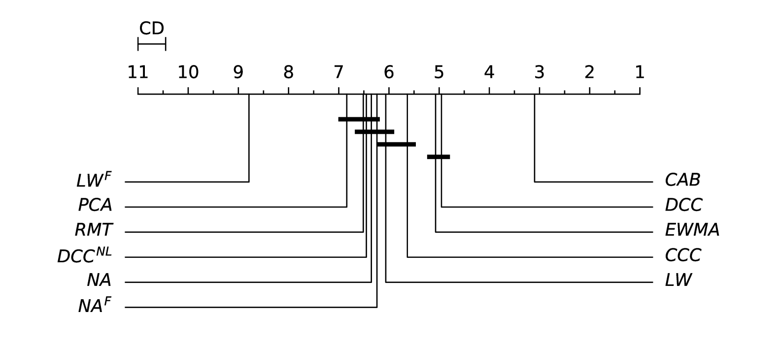
(a) Upper Triangular Euclidean distance

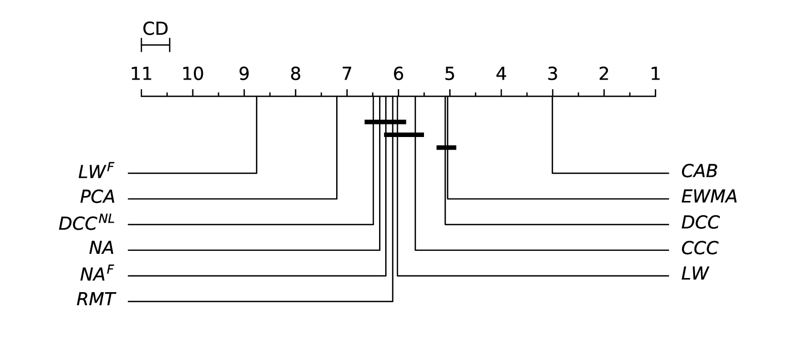
(b) Frobenius distance

Figure 1: Critical distance diagrams for the post-hoc Nemenyi test.

Table 3 presents the average distance metrics for the testing period across three market regimes: Bull-1, Bear, and Bull-2. Overall, the $CAB$ model consistently outperforms all benchmarks.

Table 3: Average Euclidean ($\mathcal{L}^{E}$) and Frobenius ($\mathcal{L}^{F}$) distances ($\times 10^{5}$) for different testing periods: Bull-1 (1 January 2021 to 2 January 2022), Bear (3 January 2022 to 12 June 2022), and Bull-2 (13 June 2022 to 31 December 2023).

	Bull-1			Bear			Bull-2
	$\mathcal{L}^{E}$	$\mathcal{L}^{F}$		$\mathcal{L}^{E}$	$\mathcal{L}^{F}$		$\mathcal{L}^{E}$	$\mathcal{L}^{F}$
$NA$	36.937	56.621		89.891	137.868		53.709	82.252
$NA^{F}$	35.680	54.992		98.002	150.780		50.586	77.545
$EWMA$	31.754	48.973		82.799	126.614		50.574	77.549
$LW$	34.126	52.599		90.441	138.173		48.089	74.088
$LW^{F}$	63.288	94.759		93.189	143.636		63.989	97.222
$CCC$	31.688	49.784		88.106	134.902		48.017	74.316
$DCC$	33.516	52.166		84.745	130.345		47.227	73.161
$DCC^{NL}$	36.779	56.449		87.650	134.167		50.767	77.734
$PCA$	37.424	57.281		90.720	139.116		54.747	83.660
$RMT$	37.246	57.083		90.638	138.821		54.493	83.411
$CAB$	24.276	37.643		66.381	102.252		39.253	60.126

While all models experience a decrease in accuracy during the turbulent Bear regime, the $CAB$ approach exhibits notable robustness. In particular, during the Bull-2 period, characterised by elevated interest rates and dynamic shifts in cross-asset relationships, integrating DL techniques with classical shrinkage enables $CAB$ to adapt effectively to changing market conditions, thereby maintaining lower distance metrics.

Supplementary Nemenyi post-hoc tests confirm that the performance improvements observed with $CAB$ are statistically significant. These tests provide further evidence that the model’s superior performance is not merely a result of sample-specific idiosyncrasies but reflects a robust ability to handle varying market regimes.

Moreover, these findings contribute to the literature on hybrid forecasting methods by demonstrating that blending modern DL with traditional econometric techniques can offer substantial gains in predictive accuracy, especially in periods of market stress. This robust performance under diverse macroeconomic conditions highlights the practical relevance of the $CAB$ approach for risk management and strategic asset allocation.

4 Robustness analysis

4.1 Impact of Using Raw Returns vs. Excess Returns

One potential criticism of our model is that it may be overly tailored to excess returns, even though some classic optimisation frameworks (Markowitz,, 1952) often use raw returns. We re-estimate our model without subtracting the risk-free rate to address this concern. All other model parameters remain identical to those described in Section 2, with the sole difference being that $\mathbf{r}_{t}$ now represents the $N$-dimensional row vector of raw daily returns for $N$ assets at time $t$.

Table 4 reports the performance of the various models under these raw returns assumptions. Our approach ($CAB$) continues outperforming all benchmarks across the entire sample and within individual market regimes, with statistically significant results based on the same post-hoc Nemenyi criteria used earlier. This finding directly informs our second research question about whether raw vs. excess returns lead to materially different covariance forecasts. When comparing Table 4 (raw returns) to Tables 2 and 3 (excess returns), the numerical magnitudes change slightly, but the rank order remains the same: $CAB$ still produces the most accurate forecasts overall.

Our findings indicate that the advantage of our framework is not contingent on the choice between excess or raw returns, reaffirming its robustness to the presence or absence of the risk-free rate. Moreover, this consistency suggests that subtracting the risk-free rate over the medium-term horizon does not significantly alter the core structure of asset co-movements. Hence, even though economic theory posits that excess returns better capture risk premiums, our empirical results show that the forecasting edge of $CAB$ holds across both raw and excess return specifications. In other words, our method retains its superior performance even when modelling raw returns, suggesting that its effectiveness does not hinge on subtracting the risk-free rate.

Table 4: Average Euclidean ($\mathcal{L}^{E}$) and Frobenius ($\mathcal{L}^{F}$) distances ($\times 10^{5}$) using raw returns for different testing periods: Overall (1 January 2021 to 31 December 2023), Bull-1 (1 January 2021 to 2 January 2022), Bear (3 January 2022 to 12 June 2022), and Bull-2 (13 June 2022 to 31 December 2023).

	Overall			Bull-1			Bear			Bull-2
	$\mathcal{L}^{E}$	$\mathcal{L}^{F}$		$\mathcal{L}^{E}$	$\mathcal{L}^{F}$		$\mathcal{L}^{E}$	$\mathcal{L}^{F}$		$\mathcal{L}^{E}$	$\mathcal{L}^{F}$
$NA$	53.525	82.020		36.936	56.620		89.895	137.875		53.707	82.249
$NA^{F}$	52.486	80.668		34.913	53.883		98.623	151.717		50.462	77.372
$EWMA$	49.174	75.441		31.753	48.972		82.798	126.613		50.697	77.730
$LW$	49.771	76.512		34.125	52.598		90.442	138.174		48.087	74.085
$LW^{F}$	68.130	103.353		63.273	94.736		93.190	143.636		63.985	97.217
$CCC$	48.508	75.106		31.599	49.634		88.139	135.038		47.948	74.196
$DCC$	48.232	74.661		33.445	52.045		84.884	130.630		47.161	73.050
$DCC^{NL}$	51.604	79.051		36.691	56.305		87.856	134.535		50.731	77.664
$PCA$	54.348	83.153		37.423	57.280		90.724	139.123		54.745	83.657
$RMT$	54.144	82.914		37.245	57.081		90.643	138.829		54.491	83.408
$CAB$	36.663	56.518		22.807	35.673		62.036	96.406		38.273	58.441

4.2 Varying Forecast Horizons

We also examine our model’s behaviour as the forecast horizon ($F$) varies. In the baseline analysis, $F=20$ days are medium-term, but many institutional investors face different time horizons for risk management or asset allocation decisions. In line with our first research question regarding underexplored medium-term horizons, we extend $F$ from 10 to 250 days, thus covering short, medium, and long horizons. To explore model performance across this range of settings, we evaluate both excess (Table LABEL:tab:diffhorizonsexc) and raw returns (Table LABEL:tab:diffhorizonsraw).

Table LABEL:tab:diffhorizonsexc shows that our model consistently achieves the lowest average distance metrics across most forecast horizons. $CAB$ remains among the top performers for shorter horizons ($F=10$). However, it does not outperform GARCH-based models ($CCC$ and $DCC$) and $EWMA$. These differences are not statistically different in the overall period, Bull-1 and Bull-2. During Bull-2, our model outperformed the benchmarks, and the results were statistically significant based on the post-hoc Nemenyi test.

For mid-term forecasting ($F=40,60,90,120,180$) for both distances, the differences are statistically significant in all periods. Thus, our model consistently outperforms the benchmarks. Please note that GARCH models tend to underperform as the forecast horizon increases, while full data models ($NA^{F}$ and $LW^{F}$) tend to diminish forecasting errors. Please note, while the $DCC^{NL}$ was more recently designed for high dimensional matrices, it provides more stable forecasts based on eigenvalues than the classical $DCC$.

At the longest horizon ($F=250$), $CAB$ again excels in most periods. Besides showing a large difference between distances during the Bear period and Bull-1, the post-hoc Nemenyi test shows no statistical difference between our model and $NA^{F}$ and $LW^{F}$, respectively. These results suggest that more complex models capture slower-moving cross-asset dynamics effectively, while classical estimators remain competitive in certain regime-specific conditions. As anticipated, naive and shrinkage methods perform relatively well at the longer horizon. These patterns reinforce our first research question’s premise that medium-term horizons can benefit from sophisticated models and highlight instances where simpler approaches hold their own.

Turning to Table LABEL:tab:diffhorizonsraw, we link our findings to the second research question: whether using raw or excess returns makes a systematic difference. Results show that the top-performing models remain consistent across all forecast horizons.

Once again, $CAB$ tends to yield the strongest overall performance. Although it does not dominate at shorter horizons, it consistently ranks near the top, showing no statistical difference between our model and the top performers. All other differences are statistically significant. These results mirror the trends seen under excess returns, indicating that the performance edge of $CAB$ does not hinge on subtracting the risk-free rate. Therefore, our DL approach remains robust even if practitioners opt for raw returns, common in certain classical optimisation frameworks. Our model performs better than the benchmarks for longer horizons ($F=250$). However, the results are not statistically different from the second-performing models ($NA^{F}$ and $LW^{F}$) for the Bull-1 and Bear periods, respectively.

These findings indicate that DL-based models can adapt effectively across different forecast windows. Across both dimensions, $CAB$ shows a stable advantage, with only minor variations in extreme horizons.

5 Economic Value in Portfolio Management

Next, we investigate the economic importance of accurate covariance forecasts in a practical asset allocation framework. Specifically, we consider an investor allocating wealth among the ETFs specified in section 3, subject to a no-short-selling constraint. Such a constraint is common among regulated institutional investors (e.g., pension funds, mutual funds) that may face limits on leverage or short positions. We adopt daily, weekly, and monthly rebalancing intervals (Symitsi et al.,, 2018).

At each rebalancing date, the investor solves the GMV problem:

$$\min_{\bm{w}_{t}}\quad\mathbf{w}_{t}^{\top}\,\widehat{\mathbf{\Sigma}}_{t}\,\mathbf{w}_{t}\quad\text{subject to}\quad\mathbf{1}^{\top}\mathbf{w}_{t}=1,\quad w_{i,t}\geq 0,$$ (43)

where $\mathbf{w}_{t}$ is an $N\times 1$ vector of GMV portfolio weights, $\widehat{\mathbf{\Sigma}}_{t}$ is the $N\times N$ forecast covariance from each model, and $\mathbf{1}$ is an $N\times 1$ vector of ones. Excluding expected returns from the optimisation allows us to isolate the impact of covariance forecasts (DeMiguel et al.,, 2009; Kourtis et al.,, 2012).

Using a rolling estimation window, we generate 11 portfolio strategies (one for each forecast model) plus an equally weighted (1/$N$) benchmark. After estimating $\widehat{\mathbf{\Sigma}}_{t}$, we compute the GMV weights and hold them until the next rebalancing date. We then record the ex-post average portfolio return for each model ($m$) as:

$$\mathbf{r}^{(m)}_{t+1}=\frac{1}{P}\sum_{t=1}^{P}\mathbf{w}^{(m)}_{t}{}^{\top}\,\mathbf{r}_{t+1},$$ (44)

where $\mathbf{r}_{t}$ is an $N\times 1$ vector of realised asset returns, $P$ is the total out-of-sample length, and $\mathbf{w}^{(m)}_{t}$ are the portfolio weights at the start of period $t$ for model $m$.

We focus on two main metrics to compare forecast models: out-of-sample portfolio variance and turnover. The variance of daily returns by a portfolio constructed by model $m$ is:

$$\sigma_{m}^{2}=\frac{1}{P}\sum_{t=1}^{P}\bigl{(}r^{(m)}_{t}-\bar{r}^{(m)}\bigr{)}^{2}$$ (45)

where $r^{(m)}_{t}$ is the ex-post return of model $m$ in period $t$, $\bar{r}^{(m)}$ and $P$ is its mean and number of observations over the out-of-sample window. Meanwhile, the average turnover reflects how often the portfolio adjusts its weights:

$$\text{TO}_{m}=\frac{1}{P-1}\sum_{t=1}^{P-1}\bigl{\lVert}\mathbf{w}_{t+1}^{(m)}-\mathbf{w}_{t+}^{(m)}\bigr{\rVert}_{1},$$ (46)

where $\mathbf{w}_{t+}^{(m)}$ are the portfolio weights of model $m$ immediately before rebalancing at $t+1$, and $\lVert\cdot\rVert_{1}$ is the 1-norm. A higher turnover implies more frequent portfolio adjustments, potentially incurring greater trading costs (Kourtis,, 2014).

We also include an equally weighted (1/$N$) portfolio, often cited for its simplicity and historically strong performance (DeMiguel et al.,, 2009). Although $1/N$ avoids estimation risk and typically maintains low turnover, it cannot adapt to shifting market correlations.

From Table 5, it is evident that the covariance forecasts provided by the $CAB$ model strike a competitive balance between risk reduction and turnover across all rebalancing horizons. Across daily, weekly, and monthly rebalancing horizons, $CAB$ slightly trails the top daily performer, approaches the leading weekly method, and matches or surpasses most other approaches monthly, thus consistently ranking among the best-performing models. This robust performance does not come at the cost of excessive turnover, as CAB’s turnover measures remain moderate compared to methods that may obtain marginally lower variances only at the expense of frequent portfolio rebalancing (e.g., $NA$, $DCC$, $DCC^{NL}$).

Table 5: performance of the global minimum variance portfolios constructed using the covariance forecasts from the 11 models under consideration plus the equal-weighted portfolio. The portfolios are compared based on their annualised out-of-sample standard deviation ($\sigma_{m}$) and average out-of-sample turnover ($\text{TO}_{m}$), respectively. Results for three different rebalancing frequencies are presented.

	Daily			Weekly			Monthly
	$\sigma_{m}^{2}$	$TO_{m}$		$\sigma_{m}^{2}$	$TO_{m}$		$\sigma_{m}^{2}$	$TO_{m}$
$1/N$	0.018132	0.005733		0.018115	0.002567		0.018060	0.001282
$NA$	0.001991	0.125568		0.002527	0.055395		0.002631	0.025707
$NA^{F}$	0.002451	0.001445		0.002453	0.000653		0.002461	0.000369
$EWMA$	0.002475	0.079388		0.002482	0.037928		0.002554	0.016088
$LW$	0.002655	0.098020		0.003373	0.047089		0.003598	0.022957
$LW^{F}$	0.002774	0.001816		0.002777	0.000956		0.002784	0.000620
$CCC$	0.002281	0.126519		0.002580	0.049839		0.002713	0.014816
$DCC$	0.002075	0.116446		0.002388	0.051710		0.002524	0.017159
$DCC^{NL}$	0.002048	0.129453		0.002448	0.056173		0.002618	0.023470
$PCA$	0.002680	0.197322		0.002722	0.072903		0.002657	0.023108
$RMT$	0.002647	0.125512		0.002689	0.055954		0.002733	0.024767
$CAB$	0.002293	0.078799		0.002428	0.048383		0.002579	0.023807

When compared to the $1/N$ benchmark, please note that all models present a statistically significant lower annual variance, based on the one-side F-Test of equalities of variance.

Examining the same metrics across distinct market regimes (Table LABEL:tab:portfoliovariancesmr) reveals that $CAB$ remains a robust contender under varying conditions: in Bull-1, it consistently competes for the lowest variance, even attaining the best performance in weekly and monthly rebalancing; in the Bear regime, $CAB$ ranks near the top in daily and weekly horizons, balancing lower turnover against marginally higher volatility than a few dynamic methods; and while Bull-2 sees other estimators occasionally surpass $CAB$, it still demonstrates stable risk control with moderate trading activity, indicating that its effectiveness persists across both tranquil and turbulent market environments.

Comparisons to the $1/N$ benchmark further highlight the importance of adaptivity. While $1/N$ offers minimal turnover, it endures noticeably higher variance in all market conditions, reflecting its inability to exploit up-to-date correlation information. Indeed, the difference in annualised variances between $CAB$ and $1/N$ can reach 80-90 basis points in certain scenarios, a gap that can substantially affect risk-adjusted returns and capital preservation.

Overall, $CAB$ tends to exhibit moderate turnover, balancing the need to adjust to changing correlations without incurring unnecessary trades. This stability benefits investors who must limit transaction costs or adhere to regulatory constraints on turnover. These results underscore that advanced covariance estimation can yield economically meaningful improvements in risk control, particularly over the medium-term horizons favoured by many institutional investors. The $CAB$ model stands out by combining strong variance reduction with stable rebalancing behaviour, balancing responsiveness to market changes and turnover efficiency.

6 Conclusion

We propose a novel DL framework for medium-term covariance forecasting in multi-asset portfolios, combining 3D convolutions, bidirectional LSTMs, and multi-head attention. Empirical tests on various ETFs from 2017 to 2023 reveal that this model, enhanced by a final shrinkage step, consistently outperforms classical benchmarks across different forecast horizons and market regimes.

Notably, its performance advantage remains robust whether one subtracts a risk-free rate from returns, suggesting broad applicability in diverse portfolio management practices.

In portfolio experiments, the proposed method enables global minimum-variance (GMV) strategies to achieve lower out-of-sample volatility with moderate turnover, underlining the tangible economic value of improved covariance estimation. By bridging cutting-edge DL techniques with established financial principles, our work highlights the promise of sophisticated spatiotemporal modelling for risk management and allocation decisions, especially at horizons where structural shifts and evolving correlations pose unique forecasting challenges.

Still, several research avenues warrant further exploration. First, extending the network architecture to accommodate skewed or heavy-tailed distributions could better capture tail risk in times of market stress. Second, explicitly incorporating transaction costs or liquidity constraints within the optimisation process might yield more realistic and implementable trading strategies. Finally, evaluating the model in larger cross-sectional settings or applied to alternative asset classes (e.g., commodities, crypto assets) would illuminate its scalability and robustness.

We hope these findings encourage the finance community to explore and adapt advanced neural architectures for medium-term and long-horizon applications, strengthening the link between machine learning innovation and effective real-world asset allocation.

Appendix A Appendix

A.1 LSTM cell detailed explanation

An LSTM (Hochreiter,, 1997) cell consists of three main gates: the forget gate ($\textbf{{f}}_{t}$), the input gate ($\textbf{{i}}_{t}$), and the output gate ($\textbf{{o}}_{t}$). They are respectively calculated as:

$$\textbf{{f}}_{t}=\sigma(\mathbf{W}_{f}.[\mathbf{h}_{(t-1)},\mathbf{x}_{t}\ ]+\mathbf{b}_{f})$$ (A.1)

$$\textbf{{i}}_{t}=\sigma(\mathbf{W}_{i}.[\mathbf{h}_{(t-1)},\mathbf{x}_{t}\ ]+\mathbf{b}_{i})$$ (A.2)

$$\textbf{{o}}_{t}=\sigma(\mathbf{W}_{o}.[\mathbf{h}_{(t-1)},\mathbf{x}_{t}\ ]+\mathbf{b}_{o})$$ (A.3)

where $\mathbf{x}_{t}$ is the vector input at time $t$, $\mathbf{h}_{(t-1)}$ is the hidden vector state, $\mathbf{W}_{f}$, $\mathbf{W}_{i}$ and $\mathbf{W}_{c}$ are weight matrices, and $\mathbf{b}_{f}$, $\mathbf{b}_{i}$ and $\mathbf{b}_{o}$ are bias vectors. The sigmoid function $\sigma$ ensures that the output values are between 0 and 1, representing how much each component should be forgotten.

The forget gate decides what information should be discarded from the cell state. Next, the input gate determines what new information should be added to the cell state. This process involves two steps: calculating the input gate Eq. (A.2) and creating new candidate values:

$$\mathbf{\widetilde{C}}_{t}=\tanh\left(\mathbf{W}_{c}\cdot\left[\mathbf{h}_{t-1},\mathbf{x}_{t}\right]+\mathbf{b}_{c}\right)$$ (A.4)

where $\mathbf{W}_{c}$ is the weight matrix, and $\mathbf{b}_{c}$ is a bias vector. The input gate modulates the extent to which new information is added to the cell state. The cell state update combines the forget gate and input gate operations to update the cell state:

$$\mathbf{C}_{t}=\textbf{{f}}_{t}\odot\mathbf{C}_{(}t-1)+\textbf{{i}}_{t}\odot\mathbf{\widetilde{C}}_{t}$$ (A.5)

This equation ensures that the cell state retains essential information over long periods.

Finally, the output gate controls what information should be outputted from the cell. This involves two steps: calculating the output gate Eq. (A.3) and determining the hidden state:

$$\mathbf{h}_{t}=\textbf{{o}}_{t}\odot\tanh{\left(\mathbf{C}_{t}\right)}$$ (A.6)

A.2 Hyperparameter Grid Search

Table A1: Hyperparameter Grid Search table.

Hyperparameter	Range
Optimiser	Adam, SGD
Batch size	32, 64, 128, 256
Learning rate	$10^{-3}$, $10^{-4}$, $10^{-5}$
Lookback window ($L$)	20, 40, 60, 80, 100, 120, 250
3D convolution kernel size ($ks$)	3, 5, 7
BiLSTM hidden dimensions ($hd$)	32, 64, 128, 256
BiLSTM stacked layers ($u$)	3, 4, 5, 6, 7
Number of heads ($he$)a	2, 4, 6, 8, 16, 32
Shrinkage factor ($\phi$)	0.00, 0.20, 0.40, 0.60, 0.80, 1.00

A.3 Extended Data Tables

Table A2: Average Euclidean ($\mathcal{L}^{E}$) and Frobenius ($\mathcal{L}^{F}$) distances ($\times 10^{5}$) using excess returns with different horizons ($F$) for different testing periods: Overall (1 January 2021 to 31 December 2023), Bull-1 (1 January 2021 to 2 January 2022), Bear (3 January 2022 to 12 June 2022), and Bull-2 (13 June 2022 to 31 December 2023).

		Overall			Bull-1			Bear			Bull-2
		$\mathcal{L}^{E}$	$\mathcal{L}^{F}$		$\mathcal{L}^{E}$	$\mathcal{L}^{F}$		$\mathcal{L}^{E}$	$\mathcal{L}^{F}$		$\mathcal{L}^{E}$	$\mathcal{L}^{F}$
$F=10$	$NA$	70.309	107.739		54.194	82.600		107.447	165.092		69.960	107.363
	$NA^{F}$	62.260	95.586		46.956	71.921		106.652	163.471		59.271	91.185
	$EWMA$	58.851	90.253		42.125	64.612		94.704	145.253		59.272	90.889
	$LW$	63.548	97.681		47.376	72.757		104.804	160.926		62.036	95.449
	$LW^{F}$	75.861	115.370		69.194	104.027		105.832	162.356		71.461	109.054
	$CCC$	58.111	89.824		42.451	65.818		95.819	147.003		57.301	88.763
	$DCC$	62.210	95.018		48.557	73.797		96.913	147.989		60.972	93.374
	$DCC^{NL}$	65.361	99.154		51.461	77.640		100.48	152.649		64.160	97.548
	$PCA$	71.266	109.164		54.984	83.752		110.811	170.301		70.323	107.864
	$RMT$	71.064	108.951		54.819	83.588		110.623	170.011		70.094	107.641
	$CAB$	56.954	87.317		44.134	67.401		94.689	145.287		54.291	83.369
$F=40$	$NA$	45.872	70.272		24.755	38.850		72.135	108.838		51.939	79.449
	$NA^{F}$	47.436	72.906		31.056	47.811		90.540	139.813		45.522	69.719
	$EWMA$	44.734	68.528		26.175	40.546		74.009	112.405		48.262	73.923
	$LW$	43.441	66.728		23.834	37.275		76.162	114.702		46.645	71.886
	$LW^{F}$	63.848	96.730		62.374	93.125		78.628	122.264		60.501	91.635
	$CCC$	43.434	67.183		27.608	43.493		75.190	114.891		44.465	68.675
	$DCC$	42.622	66.124		27.194	42.996		73.983	113.348		43.509	67.391
	$DCC^{NL}$	43.764	67.604		28.135	44.201		75.173	114.919		44.767	69.024
	$PCA$	46.390	71.007		24.934	39.238		72.294	109.567		52.781	80.410
	$RMT$	46.177	70.771		24.796	39.028		72.411	109.269		52.424	80.176
	$CAB$	22.851	35.411		13.091	20.268		42.372	65.754		23.505	36.408
$F=60$	$NA$	44.053	68.114		26.115	42.593		72.110	109.681		47.531	72.584
	$NA^{F}$	45.519	69.961		30.907	47.659		83.084	128.667		44.068	67.348
	$EWMA$	44.704	68.490		26.626	41.728		74.557	112.995		47.751	72.910
	$LW$	42.035	65.084		24.836	40.385		75.018	113.948		43.600	66.895
	$LW^{F}$	62.001	93.989		62.649	93.590		69.286	108.383		59.458	90.055
	$CCC$	42.647	66.037		29.089	45.917		68.525	105.242		43.916	67.686
	$DCC$	40.986	63.934		26.426	42.585		69.459	106.517		42.150	65.398
	$DCC^{NL}$	42.268	65.595		27.106	43.443		71.582	109.283		43.579	67.259
	$PCA$	44.550	68.801		26.466	43.142		72.705	111.010		48.096	73.173
	$RMT$	44.334	68.575		26.291	42.936		72.803	110.768		47.761	72.940
	$CAB$	22.305	34.990		12.842	20.226		39.166	62.879		23.540	36.458
$F=90$	$NA$	43.972	68.530		30.179	49.646		76.424	117.032		43.479	66.670
	$NA^{F}$	43.572	67.004		30.527	47.207		83.143	128.419		40.520	61.975
	$EWMA$	44.720	68.781		28.925	45.742		73.402	111.890		46.624	71.190
	$LW$	42.446	66.204		28.694	47.283		79.704	121.665		40.527	62.340
	$LW^{F}$	60.006	91.073		61.704	92.289		64.055	100.713		57.724	87.477
	$CCC$	43.390	67.342		32.735	51.757		68.495	105.076		42.999	66.475
$F=90$	$DCC$	40.234	63.342		29.961	48.303		65.688	101.473		39.492	62.005
	$DCC^{NL}$	42.615	66.462		29.762	48.148		71.380	108.855		42.584	66.011
	$PCA$	44.464	69.171		30.520	50.091		76.867	118.267		44.085	67.265
	$RMT$	44.239	68.951		30.343	49.925		77.105	118.060		43.693	67.005
	$CAB$	13.977	21.752		10.080	16.184		20.742	32.133		14.538	22.346
$F=120$	$NA$	48.590	75.398		36.397	59.019		84.342	128.425		46.097	70.593
	$NA^{F}$	41.909	64.465		31.713	49.127		84.615	129.958		36.093	55.352
	$EWMA$	45.330	69.861		33.556	53.195		71.953	109.497		45.222	69.142
	$LW$	47.098	73.175		34.956	56.786		87.296	132.635		43.277	66.502
	$LW^{F}$	58.216	88.420		60.114	90.286		64.569	100.736		55.133	83.621
	$CCC$	44.163	68.631		36.440	57.692		71.518	108.718		41.212	64.060
	$DCC$	40.946	64.563		33.741	54.358		68.094	104.261		37.719	59.629
	$DCC^{NL}$	44.082	68.671		34.120	54.937		74.174	112.239		41.789	64.902
	$PCA$	49.115	76.015		36.715	59.374		84.740	129.651		46.794	71.202
	$RMT$	48.867	75.827		36.519	59.220		85.041	129.486		46.352	70.985
	$CAB$	12.635	19.816		10.718	17.319		18.659	29.190		12.125	18.707
$F=180$	$NA$	57.475	88.882		50.083	79.438		92.682	140.191		52.022	80.073
	$NA^{F}$	38.460	59.180		32.171	49.910		82.117	124.805		29.829	46.088
	$EWMA$	50.035	77.019		43.437	68.307		76.903	116.122		46.487	71.288
	$LW$	56.137	86.937		49.005	77.757		94.604	142.932		49.567	76.591
	$LW^{F}$	54.308	82.570		54.261	81.972		45.646	95.111		52.187	79.306
	$CCC$	44.949	70.232		40.531	64.242		72.901	110.150		39.678	62.498
	$DCC$	46.528	72.381		41.217	65.244		75.945	114.305		41.410	64.807
	$DCC^{NL}$	46.532	72.386		41.220	65.248		75.950	114.312		41.414	64.812
	$PCA$	58.026	89.446		50.494	79.976		92.884	141.079		52.765	80.559
	$RMT$	57.744	89.294		50.351	79.843		93.189	140.964		52.223	80.384
	$CAB$	12.356	19.146		11.116	17.602		18.159	27.468		11.472	17.726
$F=250$	$NA$	76.850	117.44		107.237	163.541		79.505	120.16		56.341	86.706
	$NA^{F}$	34.002	52.367		33.076	51.123		64.126	97.309		25.830	40.087
	$EWMA$	53.737	82.720		53.030	82.554		72.648	109.762		48.689	74.953
	$LW$	74.903	114.697		103.984	158.986		80.825	122.029		54.291	83.797
	$LW^{F}$	49.653	75.499		47.293	71.542		45.646	70.522		52.353	79.519
	$CCC$	43.487	68.479		42.628	67.459		58.966	89.895		39.537	62.904
	$DCC$	40.299	64.494		38.892	62.869		53.375	82.622		37.405	60.269
	$DCC^{NL}$	40.223	66.604		49.514	77.717		81.610	120.697		22.135	43.633
	$PCA$	77.628	118.284		108.476	165.211		79.544	120.791		57.035	87.075
	$RMT$	77.315	118.139		108.26	165.074		79.841	120.668		56.481	86.919
	$CAB$	16.116	24.758		22.511	34.543		16.201	24.572		11.938	18.457

Table A3: Average Euclidean ($\mathcal{L}^{E}$) and Frobenius ($\mathcal{L}^{F}$) distances ($\times 10^{5}$) using raw returns with different horizons ($F$) for different testing periods: Overall (1 January 2021 to 31 December 2023), Bull-1 (1 January 2021 to 2 January 2022), Bear (3 January 2022 to 12 June 2022), and Bull-2 (13 June 2022 to 31 December 2023).

		Overall			Bull-1			Bear			Bull-2
		$\mathcal{L}^{E}$	$\mathcal{L}^{F}$		$\mathcal{L}^{E}$	$\mathcal{L}^{F}$		$\mathcal{L}^{E}$	$\mathcal{L}^{F}$		$\mathcal{L}^{E}$	$\mathcal{L}^{F}$
$F=10$	$NA$	70.309	107.739		54.193	82.599		107.449	165.094		69.959	107.362
	$NA^{F}$	62.057	95.297		46.340	71.028		107.068	164.102		59.155	91.020
	$EWMA$	58.908	90.338		42.125	64.612		94.704	145.253		59.384	91.053
	$LW$	63.547	97.680		47.376	72.755		104.804	160.927		62.035	95.448
	$LW^{F}$	75.854	115.361		69.181	104.007		105.831	162.355		71.457	109.048
	$CCC$	58.092	89.783		42.384	65.733		95.843	147.035		57.300	88.730
	$DCC$	62.186	94.973		48.470	73.686		96.894	147.968		60.986	93.364
	$DCC^{NL}$	65.338	99.111		51.367	77.516		100.447	152.608		64.186	97.557
	$PCA$	71.265	109.164		54.983	83.750		110.813	170.304		70.322	107.863
	$RMT$	71.064	108.951		54.818	83.587		110.625	170.014		70.093	107.640
	$CAB$	58.272	89.475		43.967	67.109		94.554	145.032		56.996	87.822
$F=40$	$NA$	45.876	70.278		24.754	38.850		72.131	108.833		51.948	79.462
	$NA^{F}$	47.200	72.577		30.161	46.526		91.426	141.121		45.386	69.534
	$EWMA$	44.796	68.618		26.174	40.545		74.005	112.399		48.383	74.100
	$LW$	43.444	66.733		23.834	37.275		76.161	114.700		46.652	71.896
	$LW^{F}$	63.845	96.725		62.359	93.102		78.638	122.279		60.502	91.636
	$CCC$	43.321	67.023		27.469	43.276		75.123	114.858		44.354	68.515
	$DCC$	42.585	66.060		27.081	42.811		74.082	113.527		43.481	67.335
	$DCC^{NL}$	43.739	67.556		28.016	44.008		75.278	115.106		44.766	69.003
	$PCA$	46.394	71.012		24.934	39.237		72.291	109.562		52.789	80.423
	$RMT$	46.181	70.777		24.796	39.027		72.408	109.265		52.432	80.188
	$CAB$	26.619	41.417		13.427	20.765		45.197	69.510		29.777	46.649
$F=60$	$NA$	44.060	68.125		26.115	42.593		72.109	109.679		47.545	72.605
	$NA^{F}$	45.268	69.612		30.016	46.385		84.049	130.081		43.879	67.086
	$EWMA$	44.759	68.570		26.625	41.727		74.548	112.981		47.861	73.069
	$LW$	42.043	65.095		24.836	40.385		75.020	113.951		43.615	66.916
	$LW^{F}$	62.000	93.988		62.634	93.568		69.301	108.405		59.462	90.061
	$CCC$	42.543	65.895		28.943	45.693		68.234	104.807		43.895	67.683
	$DCC$	39.404	61.909		26.764	42.978		64.589	100.135		40.279	63.072
	$DCC^{NL}$	42.240	65.544		27.015	43.295		71.326	108.855		43.658	67.380
	$PCA$	44.557	68.811		26.466	43.142		72.705	111.009		48.109	73.194
	$RMT$	44.341	68.586		26.291	42.935		72.803	110.767		47.775	72.961
	$CAB$	24.079	37.328		13.698	21.649		43.977	68.513		25.026	38.428
$F=90$	$NA$	43.982	68.545		30.179	49.646		76.435	117.049		43.496	66.694
	$NA^{F}$	43.314	66.645		29.713	46.043		84.231	130.003		40.232	61.574
	$EWMA$	44.761	68.841		28.925	45.742		73.405	111.893		46.704	71.306
	$LW$	42.457	66.219		28.694	47.283		79.715	121.682		40.544	62.365
	$LW^{F}$	60.007	91.075		61.690	92.268		64.073	100.740		57.731	87.486
	$CCC$	43.276	67.199		32.551	51.513		68.021	104.421		43.036	66.546
	$DCC$	40.134	63.219		29.870	48.186		65.191	100.793		39.503	62.039
	$DCC^{NL}$	42.532	66.357		29.680	48.045		70.880	108.147		42.622	66.080
	$PCA$	44.474	69.186		30.520	50.092		76.878	118.284		44.100	67.288
	$RMT$	44.249	68.966		30.343	49.925		77.116	118.077		43.709	67.029
	$CAB$	14.661	23.076		10.115	16.203		22.040	34.086		15.465	24.333
$F=120$	$NA$	48.604	75.417		36.397	59.018		84.366	128.460		46.116	70.620
	$NA^{F}$	41.664	64.124		31.048	48.181		85.754	131.620		35.717	54.821
	$EWMA$	45.361	69.908		33.555	53.194		71.959	109.504		45.282	69.232
	$LW$	47.111	73.194		34.955	56.785		87.320	132.670		43.296	66.530
	$LW^{F}$	58.219	88.425		60.101	90.267		64.599	100.781		55.138	83.629
	$CCC$	44.126	68.610		36.335	57.587		71.120	108.182		41.325	64.245
$F=120$	$DCC$	43.988	68.569		34.032	54.862		73.636	111.512		41.819	64.965
	$DCC^{NL}$	44.025	68.619		34.051	54.887		73.690	111.582		41.864	65.025
	$PCA$	49.129	76.034		36.715	59.373		84.764	129.686		46.813	71.230
	$RMT$	48.881	75.846		36.519	59.219		85.065	129.521		46.371	71.013
	$CAB$	12.118	18.831		9.496	15.248		17.864	27.435		12.147	18.653
$F=180$	$NA$	57.494	88.910		50.085	79.441		92.730	140.261		52.044	80.105
	$NA^{F}$	38.294	58.953		31.839	49.444		83.328	126.577		29.370	45.434
	$EWMA$	50.062	77.060		43.438	68.309		76.943	116.140		46.536	71.363
	$LW$	56.156	86.964		49.007	77.759		94.651	143.001		49.589	76.623
	$LW^{F}$	54.314	82.579		54.255	81.962		61.748	95.188		52.188	79.307
	$CCC$	44.844	70.073		40.368	64.069		72.299	109.109		39.755	62.603
	$DCC$	46.364	72.137		41.041	65.057		75.312	113.195		41.391	64.777
	$DCC^{NL}$	46.406	72.191		41.077	65.104		75.366	113.267		41.432	64.830
	$PCA$	58.045	89.474		50.496	79.979		92.932	141.148		52.787	80.592
	$RMT$	57.763	89.322		50.352	79.846		93.237	141.034		52.245	80.416
	$CAB$	12.828	19.854		11.180	17.728		20.372	30.851		11.702	18.031
$F=250$	$NA$	76.900	117.511		107.237	163.540		79.568	120.252		56.420	86.818
	$NA^{F}$	34.000	52.376		33.222	51.351		65.353	99.107		25.373	39.432
	$EWMA$	53.792	82.799		53.034	82.561		72.673	109.796		48.785	75.090
	$LW$	74.952	114.767		103.983	158.985		80.888	122.122		54.369	83.906
	$LW^{F}$	49.692	75.555		47.295	71.544		45.710	70.616		52.408	79.599
	$CCC$	43.349	68.233		42.431	67.189		58.278	88.611		39.597	62.977
	$DCC$	40.167	64.257		38.751	62.682		52.667	81.284		37.446	60.321
	$DCC^{NL}$	40.261	66.455		49.351	77.363		80.796	119.188		22.552	44.012
	$PCA$	77.678	118.355		108.475	165.210		79.607	120.884		57.115	87.187
	$RMT$	77.365	118.210		108.260	165.073		79.904	120.760		56.560	87.032
	$CAB$	18.246	27.828		29.049	44.148		14.976	22.681		12.182	18.727

Table A4: Performance of the GMV portfolios constructed using the covariance forecasts from the 11 models under consideration plus the equal-weighted portfolio for the different market regimes. The portfolios are compared based on their annualised out-of-sample standard deviation ($\sigma_{m}$) and average out-of-sample turnover ($\text{TO}_{m}$), respectively.

		Daily			Weekly			Monthly
		$\sigma_{m}^{2}$	$TO_{m}$		$\sigma_{m}^{2}$	$TO_{m}$		$\sigma_{m}^{2}$	$TO_{m}$
Bull-1	$1/N$	0.009883	0.005169		0.009873	0.002335		0.009907	0.001103
	$NA$	0.000543	0.150112		0.000794	0.060372		0.000834	0.026885
	$NA^{F}$	0.000731	0.001378		0.000732	0.000607		0.000736	0.000327
	$EWMA$	0.000735	0.088541		0.000748	0.043884		0.000754	0.015613
	$LW$	0.001054	0.091979		0.001572	0.044883		0.001692	0.022283
	$LW^{F}$	0.000780	0.001228		0.000781	0.000610		0.000783	0.000349
	$CCC$	0.000620	0.119486		0.000681	0.053221		0.000728	0.013605
	$DCC$	0.000529	0.207262		0.000698	0.093558		0.000781	0.024324
	$DCC^{NL}$	0.000522	0.217432		0.000784	0.097809		0.000875	0.034673
	$PCA$	0.000850	0.236835		0.000827	0.090803		0.000795	0.020906
	$RMT$	0.000856	0.150601		0.000860	0.067402		0.000826	0.025859
	$CAB$	0.000634	0.086489		0.000656	0.055931		0.000707	0.023736
Bear	$1/N$	0.029939	0.007221		0.029940	0.003443		0.029793	0.001599
	$NA$	0.002207	0.092111		0.002682	0.032018		0.002959	0.018142
	$NA^{F}$	0.002891	0.001650		0.002892	0.000935		0.002906	0.000436
	$EWMA$	0.002908	0.079065		0.002843	0.036314		0.003120	0.019997
	$LW$	0.003118	0.095723		0.003970	0.041663		0.004754	0.021610
	$LW^{F}$	0.003196	0.002035		0.003197	0.001043		0.003201	0.000570
	$CCC$	0.002497	0.129487		0.002646	0.043843		0.002590	0.012451
	$DCC$	0.002355	0.067768		0.002639	0.015372		0.002636	0.005911
	$DCC^{NL}$	0.002269	0.083567		0.002652	0.024277		0.002730	0.010308
	$PCA$	0.002800	0.114256		0.002792	0.043637		0.002864	0.011111
	$RMT$	0.002983	0.094396		0.002896	0.037508		0.003153	0.023308
	$CAB$	0.002273	0.030506		0.002464	0.022686		0.002656	0.016836
Bull-2	$1/N$	0.019967	0.005666		0.019956	0.002382		0.019933	0.001334
	$NA$	0.002823	0.118997		0.003526	0.053457		0.003667	0.029686
	$NA^{F}$	0.003398	0.001426		0.003400	0.000577		0.003406	0.000261
	$EWMA$	0.003432	0.073812		0.003433	0.034460		0.003630	0.016887
	$LW$	0.003512	0.102531		0.004274	0.048313		0.004245	0.020765
	$LW^{F}$	0.003874	0.002113		0.003879	0.001123		0.003889	0.000788
	$CCC$	0.003233	0.129874		0.003635	0.047812		0.003671	0.015276
	$DCC$	0.002947	0.071444		0.003294	0.026871		0.003364	0.009476
	$DCC^{NL}$	0.002924	0.085242		0.003318	0.034070		0.003365	0.012661
	$PCA$	0.003793	0.194898		0.003678	0.063899		0.003597	0.024379
	$RMT$	0.003668	0.118539		0.003720	0.055498		0.003762	0.029837
	$CAB$	0.003323	0.087821		0.003547	0.052596		0.003885	0.029487

References

- Akiba et al., (2019) Akiba, T., Sano, S., Yanase, T., Ohta, T., and Koyama, M. (2019). Optuna: A next-generation hyperparameter optimization framework. In Proceedings of the 25th ACM SIGKDD International Conference on Knowledge Discovery & Data Mining, pages 2623–2631. ACM.
- Baillie and Bollerslev, (1992) Baillie, R. T. and Bollerslev, T. (1992). Prediction in dynamic models with time-dependent conditional variances. Journal of Econometrics, 52(1):91–113.
- Bollerslev, (1990) Bollerslev, T. (1990). Modelling the coherence in short-run nominal exchange rates: A multivariate generalized arch model. The Review of Economics and Statistics, 72(3):498–505.
- Bollerslev et al., (2018) Bollerslev, T., Patton, A. J., and Quaedvlieg, R. (2018). Modeling and forecasting (un)reliable realized covariances for more reliable financial decisions. Journal of Econometrics, 207(1):71–91.
- Chiriac and Voev, (2011) Chiriac, R. and Voev, V. (2011). Modelling and forecasting multivariate realized volatility. Journal of Applied Econometrics, 26(6):922–947.
- Cont, (2001) Cont, R. (2001). Empirical properties of asset returns: stylized facts and statistical issues. Quantitative Finance, 1(2):223.
- Corsi, (2009) Corsi, F. (2009). A simple approximate long-memory model of realized volatility. Journal of Financial Econometrics, 7(2):174–196.
- De Nard et al., (2022) De Nard, G., Engle, R. F., Ledoit, O., and Wolf, M. (2022). Large dynamic covariance matrices: Enhancements based on intraday data. Journal of Banking & Finance, 138:106426.
- De Nard et al., (2021) De Nard, G., Ledoit, O., and Wolf, M. (2021). Factor models for portfolio selection in large dimensions: The good, the better and the ugly. Journal of Financial Econometrics, 19(2):236–257.
- De Nard et al., (2024) De Nard, G., Ledoit, O., and Wolf, M. (2024). Improved tracking-error management for active and passive investing. Available at SSRN 4898624.
- DeMiguel et al., (2009) DeMiguel, V., Garlappi, L., Nogales, F. J., and Uppal, R. (2009). A generalized approach to portfolio optimization: Improving performance by constraining portfolio norms. Management Science, 55:798–812.
- Demsar, (2006) Demsar, J. (2006). Statistical comparisons of classifiers over multiple data sets. J. Mach. Learn. Res., 7:1–30.
- Elton and Gruber, (1973) Elton, E. J. and Gruber, M. J. (1973). Estimating the dependence structure of share prices–implications for portfolio selection. The Journal of Finance, 28(5):1203–1232.
- Engle, (2002) Engle, R. (2002). Dynamic conditional correlation. Journal of Business & Economic Statistics, 20(3):339–350.
- Engle and Sheppard, (2001) Engle, R. F. and Sheppard, K. (2001). Theoretical and empirical properties of dynamic conditional correlation multivariate garch. Working Paper 8554, National Bureau of Economic Research.
- Gu et al., (2020) Gu, S., Kelly, B., and Xiu, D. (2020). Empirical asset pricing via machine learning. The Review of Financial Studies, 33:2223–2273.
- Hansen, (1994) Hansen, B. E. (1994). Autoregressive conditional density estimation. International Economic Review, 35(3):705–730.
- Harvey, (1997) Harvey, A. (1997). Trends, cycles and autoregressions. The Economic Journal, 107(440):192–201.
- Hochreiter, (1997) Hochreiter, S. (1997). Long short-term memory. Neural Computation MIT-Press.
- J.P.Morgan, (1996) J.P.Morgan (1996). Riskmetrics technical document. Morgan Guaranty Trust Company of New York.
- Kim et al., (2023) Kim, I., Lee, M., and Seok, J. (2023). Icegan: inverse covariance estimating generative adversarial network. Machine Learning: Science and Technology, 4:025008.
- Kourtis, (2014) Kourtis, A. (2014). On the distribution and estimation of trading costs. Journal of Empirical Finance, 28:104–117.
- Kourtis et al., (2012) Kourtis, A., Dotsis, G., and Markellos, R. N. (2012). Parameter uncertainty in portfolio selection: Shrinking the inverse covariance matrix. Journal of Banking & Finance, 36(9):2522–2531.
- Laloux et al., (2000) Laloux, L., Cizeau, P., Potters, M., and Bouchaud, J.-P. (2000). Random matrix theory and financial correlations. International Journal of Theoretical and Applied Finance, 03:391–397.
- Lecun et al., (1998) Lecun, Y., Bottou, L., Bengio, Y., and Haffner, P. (1998). Gradient-based learning applied to document recognition. Proceedings of the IEEE, 86(11):2278–2324.
- Ledoit and Wolf, (2003) Ledoit, O. and Wolf, M. (2003). Improved estimation of the covariance matrix of stock returns with an application to portfolio selection. Journal of Empirical Finance, 10(5):603–621.
- Ledoit and Wolf, (2004) Ledoit, O. and Wolf, M. (2004). A well-conditioned estimator for large-dimensional covariance matrices. Journal of Multivariate Analysis, 88(2):365–411.
- Ledoit and Wolf, (2020) Ledoit, O. and Wolf, M. (2020). Analytical nonlinear shrinkage of large-dimensional covariance matrices. The Annals of Statistics, 48(5):3043 – 3065.
- Ledoit and Wolf, (2022) Ledoit, O. and Wolf, M. (2022). The power of (non-)linear shrinking: A review and guide to covariance matrix estimation. Journal of Financial Econometrics, 20:187–218.
- Liu and Guo, (2019) Liu, G. and Guo, J. (2019). Bidirectional lstm with attention mechanism and convolutional layer for text classification. Neurocomputing, 337:325–338.
- Markowitz, (1952) Markowitz, H. (1952). Portfolio selection. The Journal of Finance, 7:77–91.
- Nazareth and Ramana Reddy, (2023) Nazareth, N. and Ramana Reddy, Y. V. (2023). Financial applications of machine learning: A literature review. Expert Systems with Applications, 219:119640.
- Olorunnimbe and Viktor, (2023) Olorunnimbe, K. and Viktor, H. (2023). Deep learning in the stock market—a systematic survey of practice, backtesting, and applications. Artificial Intelligence Review, 56(3):2057–2109.
- Reis et al., (2024) Reis, P., Serra, A. P., and Gama, J. (2024). The role of deep learning in financial asset management: A systematic review. Authorea, Inc.
- Robert F. Engle and Wolf, (2019) Robert F. Engle, O. L. and Wolf, M. (2019). Large dynamic covariance matrices. Journal of Business & Economic Statistics, 37(2):363–375.
- Sandoval and Franca, (2012) Sandoval, L. and Franca, I. D. P. (2012). Correlation of financial markets in times of crisis. Physica A: Statistical Mechanics and its Applications, 391(1):187–208.
- Symitsi et al., (2018) Symitsi, E., Symeonidis, L., Kourtis, A., and Markellos, R. (2018). Covariance forecasting in equity markets. Journal of Banking & Finance, 96:153–168.
- Vaswani et al., (2017) Vaswani, A., Shazeer, N. M., Parmar, N., Uszkoreit, J., Jones, L., Gomez, A. N., Kaiser, L., and Polosukhin, I. (2017). Attention is all you need. In Neural Information Processing Systems.
- Zhang et al., (2024) Zhang, C., Pu, X., Cucuringu, M., and Dong, X. (2024). Graph-based methods for forecasting realized covariances. Journal of Financial Econometrics, page nbae026.