Self-interacting processes via Doob conditioning
Abstract
We connect self-interacting processes, that is, stochastic processes where transitions depend on the time spent by a trajectory in each configuration, to Doob conditioning. In this way we demonstrate that Markov processes with constrained occupation measures are realised optimally by self-interacting dynamics. We use a tensor network framework to guide our derivations. We illustrate our general results with new perspectives on well-known examples of self-interacting processes, such as random walk bridges, excursions, and forced excursions.
I Introduction
A self-interacting process (SIP) is a stochastic process whose transition probabilities at any time depend on the empirical occupation of configurations up to that time (i.e., on the fraction of time spent by the current trajectory in the configurations of the system under consideration). In this way, the behaviour of the trajectories of a SIP is shaped by how frequently it has visited past configurations. This type of dynamics extends beyond the traditional framework of Markov processes, aiming to capture more complex, memory-dependent systems that frequently arise in real-world contexts. For instance, the dynamics of autochemotactic processes [1, 2, 3, 4, 5, 6] (self-guided entities like ants navigating towards food in response to their own chemical secretions) can be modelled by SIPs. Alternatively, while the underlying microscopic dynamics may be fully Markovian, under coarse-graining, or due to measurement limitations or incomplete data, memory effects can emerge [7, 8, 9, 10, 11], giving rise to effective dynamics that may be described by a SIP.
The study of SIPs, particularly their long-time behaviour, has been an active area of research in probability. Notable examples discussed in the survey [12] include reinforced random walks (on edges or nodes), self-avoiding walks, and self-interacting Markov chains. Self-avoiding walks [13] have practical applications in polymer physics, while self-interacting Markov chains have been used to model population dynamics in biology [12], and are highly valuable in improving the performance of Monte Carlo methods for sampling quasi-stationary distributions [14, 15, 16]. These models have also been extended to continuous-time dynamics, which in the Brownian case are referred to as self-interacting diffusions. This extension, explored in Refs. [17, 18, 19, 20, 21, 22, 23], builds on a dynamical systems framework known as stochastic approximation [24].
In this paper we show how non-Markovian SIPs can be understood in terms of the rare events of Markovian processes within the framework of Doob conditioning [25, 26, 27, 28, 29]. Specifically, we show that if a Markovian process whose trajectory measure is either conditioned or biased (viz. it is subject to either a hard or a soft condition) through its empirical occupation measure, then the optimal sampling dynamics (i.e., the unconditioned dynamics that most efficiently reproduces the condition, also known as the “Doob” dynamics [29]) can be formulated as a SIP. We illustrate this perspective with simple examples where the unconditioned dynamics is that of a fair binary coin, meaning that the dynamics of the empirical occupation is that of an unbiased random walk (RW): using our general approach it is easy to see that well-studied problems like RW bridges and excursions [30, 31, 32, 33, 34, 35, 36, 37] can be interpreted as instances of SIPs.
The paper is organised as follows. In Sec. II we establish our notation for the discrete time and discrete state settings that we consider, and define SIPs in this context. In Sec. III we introduce the trajectory observables used for both hard (cf. microcanonical) and soft (cf. canonical) trajectory conditioning. We also define the tensor network notation and visualisation that we use as a conceptually simple way to complement our analytical results on the connection between conditioning and non-Markovian dynamics. In Sec. IV we derive our central result using Doob conditioning. Section V presents three illustrative examples related to conditioned random walks. We conclude in Sec. VI with a summary and discussion.
II Self-interacting processes in discrete time
II.1 Original unbiased dynamics
We consider a discrete-time Markov chain [38] , where takes values in a finite, discrete state space of cardinality . The probabilities of transitioning between any two states and are encapsulated in the transition probability matrix , with elements defined as the conditional probabilities
| (1) |
such that for all , with
| (2) |
and where we use the symbol to indicate “probability of ”. We assume for simplicity that the transition probabilities are independent of time (i.e., independent of the step in the chain). The initial state of a trajectory is drawn from an initial probability distribution, , with
| (3) |
We denote by the sample space of the Markov chain, which we alternatively call trajectory space, for a (finite) time horizon (i.e., the overall time extent of trajectories). This is given by the -fold tensor product of the state space, . Each represents a possible sequence of states (together with the initial state) under the dynamics defined by Eq. (1) up to time . Using the Markov property, the probability of a trajectory factorises as
| (4) |
II.2 Empirical occupation measure
An important dynamical quantity in what follows will be the empirical occupation measure [39]. This refers to the trajectory-dependent (and time-dependent) probability of configurations as inferred from that trajectory at each time. It is computed from the number of visits to each configuration in the trajectory. Specifically,
| (5) |
The empirical takes values in which is a discrete subset of the simplex (filling the simplex only in the limit). It is also by definition normalised, , for all and all . The set of empiricals along a trajectory are related via the recursion
| (6) |
where in the equation above is the portion of trajectory up to time .
II.3 Self-interacting processes
We define a self-interacting chain as a stochastic process, also with state space , but where the transition rates depend not only on the current and next state, as in a Markov chain, but also on the empirical occupation at that time. That is, if up to time the current trajectory is , then the transition probabilities at time have the general form
| (7) |
The function above is a mapping from the space to , in contrast to the Markovian Eq. (1) which maps to . With the definition (7), is a transition matrix that is indexed by the empirical occupation measure as in Ref. [14].
It is important to note that while the sequence is no longer a Markov chain, the joint process can be described as a (in general time-inhomogeneous) Markov chain in the extended state space . Such a property is key for deriving the main result of this paper, as well as for describing the dynamics of SIPs in tensor network language, as shown in the following section.
III Conditioning observables and tensor network framework
III.1 Observables: hard and soft conditioning
We consider again the original Markov chain of Sec. II.A. We introduce the trajectory observable
| (8) |
where the functions , which may explicitly depend on time, map into .
III.1.1 Hard conditioning
In the case of hard conditioning we require the -dimensional observable Eq. (8) to satisfy a hard constraint. Given a -dimensional set of segments on the real line, , with , we impose the condition
| (9) |
The above imposes dynamical constraints on the process . The conditioned process must therefore evolve such that at each time step the empirical measure satisfies (9). In the language of statistical mechanics, for a trajectory ensemble this is analogous to working within a micro-canonical ensemble of configurations, where specific constraints must be strictly adhered to.
III.1.2 Soft conditioning
We may alternatively require the -dimensional observable (8) only satisfies Eq. (9) approximately. We can do this by reweighting the probability of trajectories of the stochastic process such that lies mostly within the desired set . We call this soft conditioning. The statistical mechanics analogy in this case is that of the canonical ensemble, where conditions are only enforced on average.
We show in Sec. IV below that the optimal sampling dynamics of a Markov process for any combination of hard and/or soft conditioning (9), with defined as in Eq. (8), is a self-interacting Markov chain.
III.2 Trajectory ensembles and tensor networks
A convenient framework for discussing problems relating to ensembles of stochastic trajectories is that of tensor networks (TNs) [40, 41, 42, 43, 44, 45], specifically matrix product states (MPSs) and matrix product operators (MPOs). While TN methods have been mostly used to study problems in quantum many-body systems [40, 41, 42, 43, 44, 45], they are gaining acceptance in classical stochastic dynamics [46, 47, 48, 49, 50, 51, 52, 53, 54, 55, 56].
It will prove helpful to consider in general classical hidden Markov processes (of which classical Markov processes are a subclass) [38]. For these, the states of the system are not assumed to be observable, and the only accessible information in a stochastic trajectory, apart from the initial and final configurations, is a signal at each transition along the trajectory (which in general may not be enough to resolve the states before and after). The transition probabilities are encoded in a rank-3 tensor
| (10) |
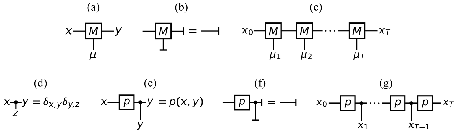
where indicates the set of possible signals. This tensor can be represented graphically as in Fig. 1(a). For a classical (hidden) Markov chain, the tensors have to be real and positive, and probability conservation requires that
| (11) |
The graphical representation of Eq. (11) as a vectorial equation is shown in Fig. 1(b): the r.h.s. is the unit or flat vector, and in the l.h.s. joined lines indicate contraction (i.e., sum over components). The ensemble of trajectories is the TN obtained by contracting the tensors (10): Fig. 1(c) shows graphically the component of the TN corresponding to the probability of the trajectory starting at , ending at and conditioned on the signals . This TN is called an MPS since once the values of the signals are fixed, the probability of the trajectory is obtained by multiplying the matrices . In TN jargon, the state space is the bond dimension and the space of signals, the physical dimension. Since we are using TNs to represent exactly the stochastic dynamics, both and are fixed by the problem under study (this is in contrast to the use of TNs as an approximate representation of functions, where the bond dimension is often used as a variational parameter).
For classical Markov chains where the states are fully observable, the signal is simply given by the states involved in the transition. Using the delta tensor, Fig. 1(d), the transition operator Fig. 1(a) can be simplified to the form shown in Fig. 1(e), its components given by the transition probabilities (1). The normalisation condition (2) is shown graphically in Fig. 1(f). By contracting the elementary tensors of Fig. 2(c), we obtain the TN that encodes the ensemble of trajectories, and whose components are the trajectory probabilities, see Fig. 1(g).
IV Generalised Doob conditioning
In this section we show how a Markov chain (as defined in Sec. II.A), conditioned on particular values of the observable as in Eq. (9), can be seen as a self-interacting Markov chain as defined in Sec. II.C. In the hard-conditioning scenario, cf. Sec. III.A.1, we write
| (12) |
where the long bar stands for “conditioned to”, whereas in the soft-conditioning scenario we introduce the notation
| (13) |
where represents the weighting function applied to favour paths close to , with a weighting that will be specified later on.
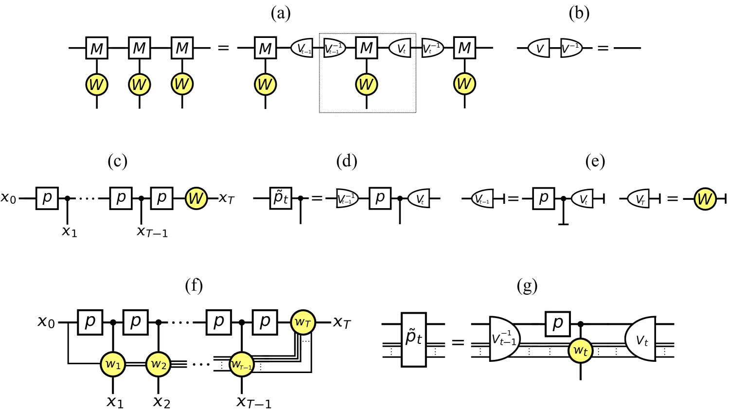
Conditioning also has a simple representation in terms of TNs. For example, the l.h.s. of Fig. 2(a) corresponds to local-in-time conditioning (or biasing) the trajectory ensemble of Fig. 1(c): the operator is diagonal in the signal, , so that for each transition in the trajectory its probability is reweigthed by a factor .
IV.1 One time Doob conditioning
Before addressing the general case, we first review Doob’s classical result for conditioning at a fixed time [25, 26] (for a modern exposition of these ideas see Ref. [29]). As will become evident, our main result in this paper is a straightforward extension of Doob’s result.
Doob’s fixed-time conditioning provides a framework for understanding how to relate a conditioned process to another process where the condition of the first is achieved automatically (i.e., without conditioning) at the price of applying an extra force. In Doob’s original setting, the Markov process has a condition on an event at some fixed time, for example reaching a particular state. Among the many ways to realise a conditioning, the Doob transform [29] is unique as it is optimal, in that it introduces only the minimal necessary perturbation to the dynamics of the original process, and the ensemble of trajectories generated by the new process is equivalent to the original trajectories post-selected to satisfy the condition.
Consider a general (hard) condition on the state of the Markov chain at the final time ,
| (14) |
If the probability of trajectory is , that of the conditioned process reads
| (15) |
where we denote by the indicator function, which is one if is true, and zero otherwise (also called a “projector”). Equation (15) is expressed as “post-selection”: one imagines generating first the trajectory through the Markov dynamics, and then keeping it or discarding it depending on whether its endpoint satisfies Eq. (14). Furthermore, note that if one wanted to define the ensemble of conditioned trajectories, then Eq. (15) also requires normalisation. Clearly, computing the conditioned ensemble in this way is highly inefficient (and, in practice, impossible in many cases).
The probability of trajectories satisfying the condition can also be written as
| (16) |
where in the first equality we used Bayes theorem, and in the second we used the Markov property and defined
| (17) |
We can define similar functions at other times for the probability of reaching the target condition at starting at state at time ,
| (18) |
These functions satisfy a backward propagation equation
| (19) |
with final condition
| (20) |
In analogy with Markov decision processes [57] we call value functions (as they encode the “value” of states in terms of the likelihood of trajectories emanating from them to reach the target). Equation (19) propagates backward in time the information (or correlations) of the condition happening at the final time . Using the value functions it is possible to derive a time-inhomogeneous Markov process , which we call the Doob process, which automatically satisfies the conditioning (14). Using the value functions, the Doob dynamics is given by time-dependent transition probabilities , which read
| (21) |
where Eq. (19) guarantees the normalisation for all and . The corresponding path probabilities are
| (22) |
where in the last equality we have used the telescopic nature of the product and Eq. (20). We note the following: (i) Eq. (22) guarantees that all trajectories of the Doob dynamics satisfy the condition (14); (ii) if we choose then Eq. (22) is the normalised conditioned probability (15); (iii) is the normalisation of Eq. (15), and plays the role of a dynamical partition function for the conditioned ensemble (and whose logarithm is the “free-energy” cost of transforming the original trajectory ensemble into the conditioned one). The above shows that by applying the Doob “force”, cf. Eq. (21), we obtain a stochastic process that optimally generates the subensemble of conditioned trajectories of the original dynamics.
IV.2 Multi-time Doob conditioning on the empirical occupations
The previous result can be extended to the case of conditioning through observables that depend on the trajectory at multiple times. We are in particular interested in (hard and/or soft) conditions like Eqs. (8) and (9) on the empirical occupation measure of the original Markov chain at all times in the trajectory.
We consider first the case of a hard constraint, cf. Sec. III.A.1. We proceed through analogous steps to those in Sec. IV.A above. We start by writing the probability of a trajectory satisfying condition (9) in a post-selection form
| (23) |
Similar to Eq. (14) for the case of single-time conditioning, Eq. (23) is not normalised over the set of conditioned trajectories. Notice that in the bottom line of Eq. (23) the trajectory constraint is sliced into local-in-time constraints.
We define a set of value functions that generalise Eq. (18), that is, give the probability of satisfying the constraints in the future starting from the current conditions,
| (24) |
Notice that in contrast to Eq. (18), the value functions defined in Eq. (24) depend both on the state and the empirical occupation at time . They obey the following backward equation
| (25) |
where is the empirical that follows from under the transition, . Since the projector appears explicitly in Eq. (25), the final condition for the backward dynamics is
| (26) |
We can now define the transition probabilities of the Doob process,
| (27) |
Equation (25) guarantees that these transition probabilities are normalised. In contrast to the case of one time conditioning, Sec. IV.A, the transition probabilities (27) depend on the empirical, and thus define a non-Markovian process. The probability of a trajectory under this dynamics is
| (28) |
where we have set the initial probability of the Doob process to be the same as that of the original process, , and we write the value function at the start, , since .
Equation (28) shows that the Doob dynamics directly generates the multi-time conditioned ensemble. However, the Doob transition probabilities (27) are of the self-interacting form (7). This is the central result of the paper, the proof that the optimal sampling dynamics of a Markov process subject to conditioning via functions of its empirical occupations is given by a non-Markovian SIP.
While we proved this result for hard conditioning, all the steps above carry through if the projectors are replaced by (possibly time dependent) weight functions that implement a soft conditioning. The examples in Sec. V illustrate both kinds of conditionings.
IV.3 Tensor network description
The results of Secs IV.A and IV.B can be easily understood using TN concepts. The l.h.s. of Fig. 2(a) shows a local-in-time conditioning/biasing. One can insert identities between the transitions given by the product of a value function and its inverse, cf. Fig. 2(b). This gives the r.h.s. of Fig. 2(a). By grouping the local tensors as shown by the dotted box in Fig. 2(a) we see that this corresponds to a gauge transformation of the TN [40, 45]. The Doob transform amounts to finding suitable value functions such that these transformed local tensors are those of a probability conserving dynamics. This gauge fixing [48] allows to absorb the local-in-time condition/bias into the (unconditioned) transition operators of a new (Doob) dynamics. Figure 2(c-e) shows this procedure for the Doob conditioning results of Sec. IV.A: panel (c) is the TN for the dynamics conditioned at the final time; panel (d) is the graphical representation of Eq. (21) (i.e., the gauge transformation of the TN); and panel (e) is the graphical representation of Eq. (19) (i.e., the gauge fixing).
As shown in Sec. IV.A, the Doob process is a Markovian dynamics in the same state space as the of the original process. This can be understood from the corresponding TNs: for local-in-time conditioning, as in Figs. 2(a) or 2(c), the MPO that is applied to the MPS that represents the trajectory ensemble is a product operator (an MPO of bond dimension one) [40, 45]. As such, the combined TN has the same bond dimension as the original TN. This is seen by comparing the dimensions traversed by a vertical cut in Fig. 1(c) vs 2(a), or Fig. 1(g) vs 2(c). That is, the conditioning does not increase the information that needs to be propagated from left to right, or in other words, the conditioned process is as Markovian as the unconditioned one.
The situation is very different for multi-time conditioning as in Sec. IV.B. Figure 2(f) shows the TN describing a condition that depends on past occupations. The biasing operator is no longer a product operator but an MPO with the bond dimension required to receive and pass forward information about visited states. It is clear that a vertical cut of the conditioned Fig. 2(f) traverses more dimensions that a vertical cut of Fig. 1(g). For conditioning dependent on the empirical occupations, cf. Eq. (23), the bond dimension of Fig. 2(f) becomes (that of the original process times that of the MPO that imposes the condition/bias). This means that in contrast to local-in-time conditioning, multi-time conditioning introduces non-Markovian effects for the dynamics in state space . The resulting generalised Doob transformation is shown in Fig. 2(g), expressed as a Markov process in an extended state space, corresponding to a TN representation of Eq. (27).
V Examples
We now illustrate our general results above with three elementary examples. For the unconditional dynamics we consider the simplest stochastic process, that of a fair coin. That is, the system has only two states, , and the transitions between states in the unconditioned dynamics have the same probability, so that the transition matrix, cf. Eq. (1), reads
| (29) |
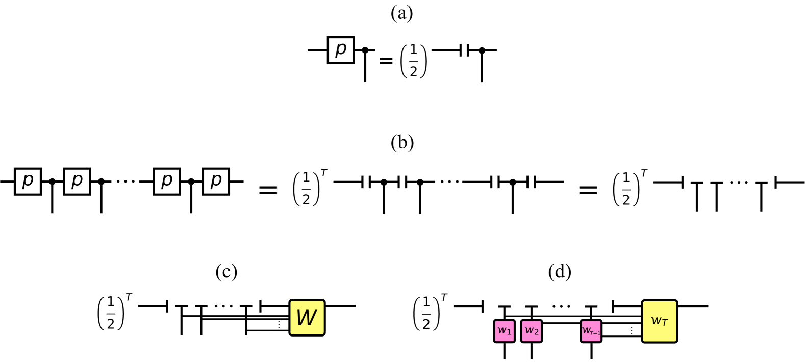
Since the matrix above has rank one, the TN that describes the dynamics reduces to a product state (an MPS with bond dimension 1), meaning that no information has to be carried along the time direction; see Fig. 3(a,b).
Below we introduce three kinds of conditions and obtain the associated SIPs that realise them optimally. For all three cases the trajectory observable (8) will have functions
| (30) |
If we interpret each flip of the coin as a step to the left or right on a one-dimensional lattice, each function gives the position after steps of an unbiased random walk (RW),
| (31) |
For trajectories up to time we have
| (32) |
Clearly, the space of the RW is isomorphic to that of the empirical occupation of the coin process, .
V.1 Random walk bridge
We consider first a hard condition, cf. Sec. III.A.1, and for Eq. (9) we choose
| (33) |
Condition (9) with Eq. (33) is automatically satisfied for since by definition. The only non-trivial condition is at the final time, . This conditions trajectories to have as many transitions to states as to , irrespective of the initial configuration (here and in what follows we assume is even). In terms of the location of the RW , this corresponds to conditioning a walker that starts at the origin to return to the origin at the final time , a process known as a random walk bridge [30, 31, 33, 35, 38].
The TN for the conditioned process is shown in Fig. 3(c). It is a special instance of the multi-time conditioning, Fig. 2(f): while the MPS of unconditioned dynamics of the coin, Fig. 3(b), is a product state with bond dimension 1, the information that needs to be propagated for the final time condition (33) increases the bond dimension in the TN of Fig. 3(c).
Given the multi-time nature of the condition, it is not possible to define the optimal sampling Doob dynamics as a Markov process in the space of the coin alone, and we need to extend to the space of the empirical occupation. In order to obtain the generalised Doob dynamics we proceed as in Sec. 4.B. The key quantities are the value functions (24). For the bridge condition, the value function at time can be obtained from the fraction of RW paths that start at and reach . Simple combinatorics gives
| (34) |
where we replace the dependence on the empirical for that of the RW given the equivalence of and , and otherwise, as the position of the walker has to be within the “light-cone” emanating from the origin for it to be able to reach the condition within the remaining time . Note that the value function is independent of the current state of the coin (a consequence of the i.i.d. nature of the unconditioned dynamics). It is easy to check that the value functions (34) satisfy the backward propagation Eq. (25). Inserting it into Eq. (27) we get the -dependent transition matrix for the Doob dynamics that generates the conditioned trajectories of the coin
| (35) |
We therefore see that a condition on the accumulated transitions of the coin being exactly balanced at the final time, Eqs. (30) and (33), is optimally realised by the SIP process Eq. (35). Futhermore, this SIP in the coin space is a Markovian process in the extended RW space : if we denote by the transition probabilities of an unbiased RW, with
| (36) |
then Eq. (35) becomes a RW with a time-dependent force,
| (37) |
The dynamics Eq. (37) is precisely that of RW bridges for time , see e.g. [35].
V.2 Random walk excursion
As a second example we consider again the fair coin with a hard condition on observable (30), but which now is non-trivial for all times. Specifically, we set
| (38) |
The final time condition is the same as in Example A, requiring the overall number of flips of the coin to be exactly balanced at time . The conditions for , however, also impose the restriction that the number of down-flips cannot exceed the number of up-flips at any time. The TN for this condition is shown in Fig. 3(d), the biasing functions being projectors, , where are the sets of Eq. (38). In terms of the RW position (i.e., of the empirical occupation), the condition forces , with at all . That is, the multi-time condition restricts the RW paths to be bridges that do not cross the origin at any time, also known as excursions [30, 31, 33, 35, 38].
As in the previous example, the value functions (24) are obtained by counting the number of paths that reach the the origin at the final time, but now also having to stay non-negative throughout. While the combinatorics leading to Eq. (34) for bridges comes from the Pascal triangle, that for the excursions comes from the Catalan triangle,
| (39) |
In this case, the Doob process for the coin is given by
| (40) |
and we see that the optimal dynamics to sample the conditioned coin process is also a SIP.
The Doob dynamics in the extended state space of the RW in this case reads
| (41) |
which implements the forces on a RW so that the trajectories are excursions.
V.3 Random walk excursion with competing forces
As a final example we consider the same hard conditioning that leads to the RW excursions above, but with an extra trajectory biasing (soft conditioning) in terms of two competing factors dependent on the empirical occupation. This combination is defined in terms of weigthing functions that depend on the observables (30),
| (42) |
where are the sets of Eq. (38), and real and arbitrary. The projector in the first factor imposes the excursion constraint. The second factor is a polynomial cost from having a balanced coin empirical occupation (i.e., a repulsion from the origin of the RW). The third factor in contrast is an exponential cost for a non-balanced coin empirical occupation (i.e., an attraction of the RW towards the origin) if (and a repulsion of the RW from the origin for ). The introduction of these extra weights creates additional correlations in the RW excursions of Sec. V.B.
The recursion relation (25) for the value functions simplifies to
| (43) |
with and where is the Heaviside step function. Additionally, we have dropped the coin state from the argument of the value function as there is no dependence on it, cf. Eqs. (34) and (39). However, in contrast to the two examples above, for this case there is no simple closed form for the solution of Eq. (43).
As before, the Doob dynamics that realises the conditioned process is a SIP in the configuration space of the coin , with transition probabilities of Eq. (27) using the value functions (43). Alternatively, the Doob dynamics can be described as a Markovian process in the RW space , with rates
| (44) |
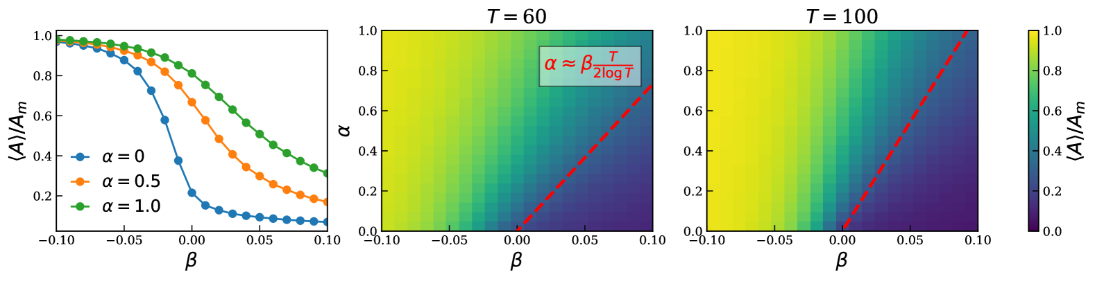
The competition between the algebraic and exponential biasing factors in Eq. (42), when , favouring large and small excursions, respectively, can give rise to a transition in the dynamics. A convenient order parameter is the area under the RW averaged over the dynamics,
| (45) |
where marks the ensemble average. takes values between a minimum of and a maximum of . This difference in scaling with suggests two possible regimes for large .
The case with was studied in the context of Fredkin spin chains in Ref. [35], where the equilibrium properties of the one-dimensional Fredkin model map to the dynamical properties of a conditioned coin with Doob dynamics corresponding to Eq. (44). Using this equivalence we know that for there is a phase transition [35] at in the limit of long time , between a phase with for , to a phase with for .
For finite the transition smoothes to a crossover occurring around . Since for large area trajectories are favoured, we expect that the crossover will move to positive , increasingly so with increasing (and becoming sharper for larger ). That is, when is positive, a larger is needed to suppress the large area trajectories in favour of the small area regime. In Fig. 4 we show results which give evidence for this behaviour (see caption for details of the numerics). Figure 4(a) shows the average rescaled area as a function of for three values of : for we recover the result of Ref. [35], corresponding to a crossover that will sharpen into a phase transition for large ; for , as increases the area grows for fixed , as expected. Figures 4(b,c) show the order parameter as a function of and for two values of : we see that there are two regimes, the large area one for small and large , and the small area one for large and small . The change appears to become sharper with larger . We can estimate the location of the crossover from a simple heuristic argument, by equating the probability of a maximum area excursion with that of a minimum area one. This gives that for large the location of the transition should obey . The dashed-red line in Figs. 4(b,c) shows that this is a reasonable estimate.
VI Conclusion
We have shown here that non-Markovian self-interacting processes, where transition probabilities depend on empirical occupations along a trajectory, in general correspond to the optimal sampling (or Doob) dynamics of a conditioned Markovian process, where the condition is non-local in time. We have also shown that this connection is made evident by representing trajectory ensembles in terms of tensor networks. We illustrated our general results with simple examples where conditioning the i.i.d. dynamics of a fair coin leads to self-interacting dynamics that in an extended space are random walks subject to time-dependent forces. We can anticipate several directions to consider following from these results. One is the study of other forms of non-Markovian dynamics and their relation to conditioned Markov processes. There should also be interesting connections to reinforcement learning problems with multi-time reward objectives. And another fruitful avenue of work should be the generalisation of the ideas here to open quantum dynamics.
Acknowledgements.
We acknowledge financial support from EPSRC grant no. EP/V031201/1.References
- Budrene and Berg [1995] E. O. Budrene and H. C. Berg, Dynamics of formation of symmetrical patterns by chemotactic bacteria, Nature 376, 49 (1995).
- Tsori and de Gennes [2004] Y. Tsori and P.-G. de Gennes, Self-trapping of a single bacterium in its own chemoattractant, Europhys. Lett. 66, 599 (2004).
- Reid et al. [2012] C. R. Reid, T. Latty, A. Dussutour, and M. Beekman, Slime mold uses an externalized spatial “memory” to navigate in complex environments, PNAS 109, 17490 (2012).
- Zhao et al. [2013] K. Zhao, B. S. Tseng, B. Beckerman, F. Jin, M. L. Gibiansky, J. J. Harrison, E. Luijten, M. R. Parsek, and G. C. Wong, Psl trails guide exploration and microcolony formation in pseudomonas aeruginosa biofilms, Nature 497, 388 (2013).
- Kranz et al. [2016] W. T. Kranz, A. Gelimson, K. Zhao, G. C. Wong, and R. Golestanian, Effective dynamics of microorganisms that interact with their own trail, Phys. Rev. Lett. 117, 038101 (2016).
- Meyer and Rieger [2021] H. Meyer and H. Rieger, Optimal non-markovian search strategies with n -step memory, Phys. Rev. Lett. 127, 070601 (2021).
- Zwanzig [2001] R. Zwanzig, Nonequilibrium Statistical Mechanics (Oxford University Press, 2001).
- Español et al. [2009] P. Español, C. Hijón, E. Vanden-Eijnden, and R. Delgado-Buscalioni, Mori–swanzig formalism as a practical computational tool, Faraday Discussions 144, 301 (2009).
- Li et al. [2015] Z. Li, X. Bian, X. Li, and G. E. Karniadakis, Incorporation of memory effects in coarse-grained modeling via the mori-zwanzig formalism, J. Chem. Phys. 143, 243128 (2015).
- Pasquale et al. [2019] N. D. Pasquale, T. Hudson, and M. Icardi, Systematic derivation of hybrid coarse-grained models, Phys. Rev. E 99 (2019).
- Brandner [2025] K. Brandner, Dynamics of microscale and nanoscale systems in the weak-memory regime, Phys. Rev. Lett. 134, 037101 (2025).
- Pemantle [2007] R. Pemantle, A survey of random processes with reinforcement, Probab. Surv. 4, 1 (2007).
- Tóth [2001] B. Tóth, Self-interacting random motions, European Congress of Mathematics , 555 (2001).
- Moral and Miclo [2007] P. D. Moral and L. Miclo, Self-interacting markov chains, Stoch. Anal. Appl. 24, 615 (2007).
- Kannan and Zhang [2008] D. Kannan and J. Zhang, Self-interacting markov chains: Some asymptotics, Stoch. Anal. Appl. 27, 196 (2008).
- Budhiraja and Waterbury [2022] A. Budhiraja and A. Waterbury, Empirical measure large deviations for reinforced chains on finite spaces, Syst. Control Lett. 169, 105379 (2022).
- Bena¨ım et al. [2002] M. Benaïm, M. Ledoux, and O. Raimond, Self-interacting diffusions, Probab. Theory Relat. Fields. 122, 1 (2002).
- Bottou [2003] L. Bottou, Stochastic learning, in Summer School on Machine Learning (Springer, 2003) pp. 146–168.
- Bena¨ım and Raimond [2005] M. Benaïm and O. Raimond, Self-interacting diffusions III. Symmetric interactions, Ann. Probab. 33, 1716 (2005).
- Kurtzmann [2010] A. Kurtzmann, The ode method for some self-interacting diffusions on , Ann. Inst. H. Poincaré Probab. Statist. 46, 618 (2010).
- Bena¨ım and Raimond [2011] M. Benaïm and O. Raimond, Self-interacting diffusions IV: Rate of convergence, Electron. J. Probab. 16, 1815 (2011).
- Chambeu and Kurtzmann [2011] S. Chambeu and A. Kurtzmann, Some particular self-interacting diffusions: ergodic behaviour and almost sure convergence, Bernoulli 17, 1248 (2011).
- Kleptsyn and Kurtzmann [2012] V. Kleptsyn and A. Kurtzmann, Ergodicity of self-attracting motion, Electron. J. Probab. 17, 1 (2012).
- Bena¨ım [1999] M. Benaïm, Dynamics of stochastic approximation algorithms (1999) pp. 1–68.
- Doob [1957] J. Doob, Conditional brownian motion and the boundary limits of harmonic functions, Bulletin de la Société Mathématique de France 85, 431 (1957).
- Doob [1984] J. L. Doob, Classical Potential Theory and Its Probabilistic Counterpart, Vol. 262 (Springer New York, 1984).
- Borkar et al. [2003] V. S. Borkar, S. Juneja, and A. A. Kherani, Peformance Analysis Conditioned on Rare Events: An Adaptive Simulation Scheme, Commun. Inf. Syst. 3, 259 (2003).
- Jack and Sollich [2010] R. L. Jack and P. Sollich, Large Deviations and Ensembles of Trajectories in Stochastic Models, Prog. Theor. Phys. Supp. 184, 304 (2010).
- Chetrite and Touchette [2015] R. Chetrite and H. Touchette, Nonequilibrium Markov processes conditioned on large deviations, Ann. H. Poincaré 16, 2005 (2015).
- Majumdar and Comtet [2005] S. N. Majumdar and A. Comtet, Airy Distribution Function: From the Area Under a Brownian Excursion to the Maximal Height of Fluctuating Interfaces, J. Stat. Phys. 119, 777 (2005).
- Majumdar [2006] S. N. Majumdar, Brownian functionals in physics and computer science, The Legacy of Albert Einstein: A Collection of Essays in Celebration of the Year of Physics , 93 (2006).
- Majumdar et al. [2008] S. N. Majumdar, J. Randon-Furling, M. J. Kearney, and M. Yor, On the time to reach maximum for a variety of constrained brownian motions, J. Phys. A: Math. Theor. 41, 365005 (2008).
- Majumdar and Orland [2015] S. N. Majumdar and H. Orland, Effective langevin equations for constrained stochastic processes, J. Stat. Mech. 2015, P06039 (2015).
- Szavits-Nossan and Evans [2015] J. Szavits-Nossan and M. R. Evans, Inequivalence of nonequilibrium path ensembles: the example of stochastic bridges, J. Stat. Mech. 2015, P12008 (2015).
- Causer et al. [2022a] L. Causer, J. P. Garrahan, and A. Lamacraft, Slow dynamics and large deviations in classical stochastic Fredkin chains, Phys. Rev. E 106, 014128 (2022a).
- Mazzolo and Monthus [2022] A. Mazzolo and C. Monthus, Conditioning two diffusion processes with respect to their first-encounter properties, J. Phys. A: Math. Theor. 55, 305002 (2022).
- Mazzolo and Monthus [2023] A. Mazzolo and C. Monthus, Joint distribution of two local times for diffusion processes with the application to the construction of various conditioned processes, J. Phys. A: Math. Theor. 56, 205004 (2023).
- Grimmett and Stirzaker [2020] G. Grimmett and D. Stirzaker, Probability and random processes (OUP, 2020).
- Touchette [2009] H. Touchette, The large deviation approach to statistical mechanics, Phys. Rep. 478, 1 (2009).
- Verstraete et al. [2008] F. Verstraete, V. Murg, and J. Cirac, Matrix product states, projected entangled pair states, and variational renormalization group methods for quantum spin systems, Adv. Phys 57, 143 (2008).
- Schollwöck [2011] U. Schollwöck, The density-matrix renormalization group in the age of matrix product states, Ann. Physics 326, 96 (2011).
- Orús [2014] R. Orús, A practical introduction to tensor networks: Matrix product states and projected entangled pair states, Ann. Physics 349, 117 (2014).
- Silvi et al. [2019] P. Silvi, F. Tschirsich, M. Gerster, J. Jünemann, D. Jaschke, M. Rizzi, and S. Montangero, The Tensor Networks Anthology: Simulation techniques for many-body quantum lattice systems, SciPost Phys. Lect. Notes , 8 (2019).
- Okunishi et al. [2022] K. Okunishi, T. Nishino, and H. Ueda, Developments in the tensor network — from statistical mechanics to quantum entanglement, J. Phys. Soc. Jpn 91, 062001 (2022).
- Bañuls [2023] M. C. Bañuls, Tensor network algorithms: A route map, Annu. Rev. Condens. Matter Phys. 14, 173 (2023).
- Gorissen et al. [2009] M. Gorissen, J. Hooyberghs, and C. Vanderzande, Density-matrix renormalization-group study of current and activity fluctuations near nonequilibrium phase transitions, Phys. Rev. E 79, 020101 (2009).
- Gorissen and Vanderzande [2012] M. Gorissen and C. Vanderzande, Current fluctuations in the weakly asymmetric exclusion process with open boundaries, Phys. Rev. E 86, 051114 (2012).
- Garrahan [2016] J. P. Garrahan, Classical stochastic dynamics and continuous matrix product states: gauge transformations, conditioned and driven processes, and equivalence of trajectory ensembles, J. Stat. Mech.: Theory Exp 2016, 073208 (2016).
- Bañuls and Garrahan [2019] M. C. Bañuls and J. P. Garrahan, Using Matrix Product States to Study the Dynamical Large Deviations of Kinetically Constrained Models, Phys. Rev. Lett. 123, 200601 (2019).
- Helms et al. [2019] P. Helms, U. Ray, and G. K.-L. Chan, Dynamical phase behavior of the single- and multi-lane asymmetric simple exclusion process via matrix product states, Phys. Rev. E 100, 022101 (2019).
- Helms and Chan [2020] P. Helms and G. K.-L. Chan, Dynamical phase transitions in a 2d classical nonequilibrium model via 2d tensor networks, Phys. Rev. Lett. 125, 140601 (2020).
- Causer et al. [2020] L. Causer, I. Lesanovsky, M. C. Bañuls, and J. P. Garrahan, Dynamics and large deviation transitions of the XOR-Fredrickson-Andersen kinetically constrained model, Phys. Rev. E 102, 052132 (2020).
- Causer et al. [2022b] L. Causer, M. C. Bañuls, and J. P. Garrahan, Finite time large deviations via matrix product states, Phys. Rev. Lett. 128, 090605 (2022b).
- Strand et al. [2022] N. E. Strand, H. Vroylandt, and T. R. Gingrich, Using tensor network states for multi-particle brownian ratchets, J. Chem. Phys 156, 221103 (2022).
- Causer et al. [2023] L. Causer, M. C. Bañuls, and J. P. Garrahan, Optimal sampling of dynamical large deviations in two dimensions via tensor networks, Phys. Rev. Lett. 130, 147401 (2023).
- Zima et al. [2025] J. P. Zima, S. B. Nicholson, and T. R. Gingrich, Chemical master equation parameter exploration using dmrg, arXiv:2501.09692 (2025).
- Sutton and Barto [2018] R. S. Sutton and A. G. Barto, Reinforcement Learning: An Introduction (A Bradford Book, Cambridge, MA, USA, 2018).