Limitations of Amplitude Encoding on Quantum Classification

Abstract

It remains unclear whether quantum machine learning (QML) has real advantages when dealing with practical and meaningful tasks. Encoding classical data into quantum states is one of the key steps in QML. Amplitude encoding has been widely used owing to its remarkable efficiency in encoding a number of $2^{n}$ classical data into $n$ qubits simultaneously. However, the theoretical impact of amplitude encoding on QML has not been thoroughly investigated. In this work we prove that under some broad and typical data assumptions, the average of encoded quantum states via amplitude encoding tends to concentrate towards a specific state. This concentration phenomenon severely constrains the capability of quantum classifiers as it leads to a loss barrier phenomenon, namely, the loss function has a lower bound that cannot be improved by any optimization algorithm. In addition, via numerical simulations, we reveal a counterintuitive phenomenon of amplitude encoding: as the amount of training data increases, the training error may increase rather than decrease, leading to reduced decrease in prediction accuracy on new data. Our results highlight the limitations of amplitude encoding in QML and indicate that more efforts should be devoted to finding more efficient encoding strategies to unlock the full potential of QML.

I Introduction

Quantum machine learning (QML) has been expected to become a new technology that can surpass its classical counterpart due to quantum advantages in representation, parallelism and entanglement Biamonte et al. (2017); Xiao et al. (2023); Azam and Kaiser (2024); Zheng et al. (2023). Classification is a standard classical machine learning task that has been extensively studied LeCun et al. (1998); Krizhevsky et al. (2012); Chen et al. (2024); Schultheis et al. (2024); Raman and Tewari (2024); Wang and Zhang (2024). Quantum classifiers Schuld et al. (2020); Pérez-Salinas et al. (2020); Henderson et al. (2020); Hubregtsen et al. (2022); Huang et al. (2021a); Xu et al. (2024); Mitsuda et al. (2024); Wang et al. (2024a); Liu et al. (2021); Jerbi et al. (2023) have attracted increasing attention and claimed advantages on some toy classical datasets Schuld et al. (2020); Pérez-Salinas et al. (2020); Henderson et al. (2020); Hubregtsen et al. (2022); Huang et al. (2021a); Xu et al. (2024); Mitsuda et al. (2024); Wang et al. (2024a) and carefully designed datasets Liu et al. (2021); Jerbi et al. (2023). Although it is widely believed that quantum classifiers outperform classical machine learning when processing quantum data Cong et al. (2019); Huang et al. (2021b, 2022), for practical classification tasks, it remains unclear whether QML has real advantage, particularly in the current noisy intermediate-scale quantum era Schuld and Killoran (2022); Cerezo et al. (2022); Lau et al. (2022).

Quantum machine learning models Schuld ; Caro et al. (2022); Huang et al. (2021a) are constructed using parameterized quantum circuits (PQCs), which consist of quantum gates with tunable parameters Benedetti et al. (2019). There have been many works investigating the limitations of QML models. Most of them focused on the trainability issues caused by the phenomena of barren plateaus McClean et al. (2018); Marrero et al. (2021); Thanasilp et al. (2023); Ragone et al. (2024) and having exponentially many spurious local minimum You and Wu (2021); Anschuetz and Kiani (2022). Various kinds of strategies, such as, appropriate parameter initialization Zhang et al. (2022); Wang et al. (2024b), symmetry-preserving ansatzes Meyer et al. (2023), tree tensor networks Huggins et al. (2019), convolutional neural networks Cong et al. (2019), local encoded cost function Cerezo et al. (2021), and over-parameterization Larocca et al. (2023) have been proposed to mitigate the training issue. Few works have investigated the generalization ability of QML Caro et al. (2022, 2021); Huang et al. (2021b), and it was proved in Ref. Caro et al. (2022) that good generalizations can be guaranteed from few data. We note that good generalization alone does not necessarily guarantee good prediction, since the training error may be large and become the dominant term in the prediction error.

Encoding classical data into quantum states is a necessary and crucial step in QML Cerezo et al. (2022); Wiebe (2020); Lloyd et al. ; Weigold et al. (2021); Rath and Date (2024). There are mainly two encoding paradigms Jerbi et al. (2023): (1) variational-encoding, where the data encoding and variational PQC are separated; (2) data re-uploading, where the data encoding and variational PQC are interleaved Pérez-Salinas et al. (2020). In this work we focus on the variational-encoding paradigm. There are three primary quantum encoding methods: basis encoding, angle encoding and amplitude encoding Schuld and Petruccione (2018). Basis encoding can only encode binary information by mapping each bit to either $|0\rangle$ or $|1\rangle$. Angle encoding embeds real numbers by mapping them to the angles of quantum rotational gates. The angle encoding is easy to implement but not efficient. Amplitude encoding encodes complex numbers by mapping them to the probability amplitudes of quantum states. Despite having significant challenges in implementing amplitude encoding in practice, it can encode a number of $2^{n}$ data into $n$ qubits simultaneously. In view of this remarkable efficiency, amplitude encoding has been widely employed to demonstrate quantum superiority on classical datasets LaRose and Coyle (2020); Grant et al. (2018); Hur et al. (2022); Mitsuda et al. (2024); Wang et al. (2024a); Li et al. (2024). However, the numerical simulations therein are mainly based on the simple MNIST dataset LeCun , which may mask the limitations of QML caused by amplitude encoding.

There are only few works concerning the relationship between the power or limitations of QML and encoding strategies. Ref. Caro et al. (2021) and Ref. Schuld et al. (2021) have respectively investigated the impact of encoding strategies on the generalization error and expressive power of QML. For the limitations of QML, it was proved in Ref. Li et al. (2022) that under reasonable assumptions, the average encoded quantum states via angle encoding concentrates to the maximally mixed state at an exponential rate as the depth of the encoding circuit increases. For quantum kernel methods which employ angle encoding to generate kernels Hubregtsen et al. (2022); Schuld and Killoran (2019); Wang et al. (2021); Thanasilp et al. (2024), it was demonstrated that for a wide range of situations, values of quantum kernels over different input data concentrate towards some fixed value exponentially as the number of qubits increases Thanasilp et al. (2024). The concentration phenomenon severely limits the power of QML. In the case of amplitude encoding, most studies have primarily focused on two aspects: how to prepare the target encoded states Giovannetti et al. (2008); Park et al. (2019); Jiang et al. (2019); Plesch and Brukner (2011); Long and Sun (2001); Araujo et al. (2021); Gonzalez-Conde et al. (2024), and how to efficiently implement approximate amplitude encoding Nakaji et al. (2022); Mitsuda et al. (2024); Daimon and Matsushita (2024).

In this work, we investigate the limitation of amplitude encoding on quantum classification. First, we prove that under certain conditions, a loss barrier phenomenon occurs, that is, the loss function has a lower bound that cannot be improved by any optimization algorithm. Then, we theoretically show that under reasonable data assumptions, the amplitude encoding satisfies the conditions for the loss barrier phenomenon. Finally, we validate our findings via numerical simulations that the amplitude encoding is prone to suffer from the loss barrier phenomenon for sophisticated and commonly encountered datasets. In machine learning a general belief is that an increase in the amount of training data generally benefits the performance. However, our numerical simulations reveal that under amplitude encoding as the amount of training data increases, although the generalization error decreases, the training error increases counterintuitively, resulting in overall poor prediction performance. This is essentially owing to the concentration phenomenon caused by the amplitude encoding. Our findings help understand the limitations of amplitude encoding in QML and highlight the need for finding more efficient encoding strategies to unlock the full power of QML.

The paper is organized as follows. In Sec. II, we introduce the amplitude encoding, and set up the framework for quantum classification. We present the main results in Sec. III, and conclude in Sec. IV.

II Preliminary and Framework

II.1 Amplitude encoding

Without loss of generality, suppose that the classical data feature $\boldsymbol{x}\in\mathbb{R}^{2^{n}}$. By amplitude encoding, we can embed the feature $\boldsymbol{x}=\left[x_{0},x_{1},\dots,x_{2^{n}-1}\right]^{\top}$ into a quantum state vector $|\phi(\boldsymbol{x})\rangle$ as

$$|\phi(\boldsymbol{x})\rangle=\frac{1}{C_{\boldsymbol{x}}}\sum_{i=0}^{2^{n}-1}x_{i}|i\rangle,$$

where $C_{\boldsymbol{x}}=\sqrt{x_{0}^{2}+x_{1}^{2}+\cdots+x_{2^{n}-1}^{2}}$ is the normalization factor. An equivalent representation in terms of the density matrix $\rho(\boldsymbol{x})$ reads

$$\rho(\boldsymbol{x}) =|\phi(\boldsymbol{x})\rangle\langle\phi(\boldsymbol{x})|$$ (1)

$$=\frac{1}{C_{\boldsymbol{x}}^{2}}\sum_{i=0}^{2^{n}-1}\sum_{j=0}^{2^{n}-1}x_{i}x_{j}|i\rangle\langle j|.$$

II.2 Quantum classifier

Consider a $K$-class classification problem. Denote the feature space by $\mathcal{X}=\mathbb{R}^{2^{n}}$ and the label space by $\mathcal{Y}=\{1,2,\dots,K\}$. Given a dataset $S=\left\{\left(\boldsymbol{x}^{(m)},y^{(m)}\right)\right\}^{M}_{m=1}$ containing $M$ independent and identically distributed ($i.i.d.$) samples, where each sample $\left(\boldsymbol{x}^{(m)},{y}^{(m)}\right)\in\mathcal{X}\times\mathcal{Y}$ obeys an unknown joint distribution $\mathcal{D}$, a quantum classifier learns from the dataset $S$ to obtain a hypothesis $h_{S}$. Our aim is to enable the hypothesis $h_{S}$ to accurately classify new, unseen samples that follow the same distribution $\mathcal{D}$.

To be specific, we embed the feature $\boldsymbol{x}^{(m)}$ into a feature quantum state $\rho\left(\boldsymbol{x}^{(m)}\right)$ through a PQC $U(\boldsymbol{\theta})$. For classification, we select $K$ fixed observables, $H_{1},\cdots,H_{K}$, each corresponding to one of the $K$ classes. These observables are typically chosen to be the tensor product of Pauli operators, such as, ${Z\otimes Y,X\otimes Y,X\otimes Y\otimes Z,\cdots}$, where $X,Y,Z$ denote Pauli matrices. The output associated with the $k$-th class is defined as

$$h_{k}\left(\boldsymbol{x}^{(m)},\boldsymbol{\theta}\right)=\operatorname{Tr}\left[H_{k}U(\boldsymbol{\theta})\rho(\boldsymbol{x}^{(m)})U^{\dagger}(\boldsymbol{\theta})\right].$$

Let

$$\hat{y}^{(m)}=\operatorname*{argmax}_{k}h_{k}(\boldsymbol{x}^{(m)},\boldsymbol{\theta}).$$

We now define the output of the learned hypothesis $h_{S}$ for the feature $\boldsymbol{x}^{(m)}$ to be

$$h_{S}(\boldsymbol{x}^{(m)})=\hat{y}^{(m)}.$$

II.3 Learning framework

To minimize the difference between the predicted label $\hat{y}^{(m)}$ of the hypothesis $h_{S}$ and the true label $y^{(m)}$ for the feature $\boldsymbol{x}^{(m)}$, we train the parameters of the quantum classifier on dataset $S=\{(\boldsymbol{x}^{(m)},y^{(m)})\}_{m=1}^{M}$ using the cross-entropy loss with the softmax function: Li et al. (2022)

$$\mathcal{L}_{S}(\boldsymbol{\theta})=\frac{1}{M}\sum_{m=1}^{M}\ell(\boldsymbol{\theta};\boldsymbol{x}^{(m)},y^{(m)}),$$ (2)

$$\ell(\boldsymbol{\theta};\boldsymbol{x}^{(m)},y^{(m)})=-\sum_{k=1}^{K}\boldsymbol{y}_{k}^{(m)}\ln\left(\frac{e^{h_{k}(\boldsymbol{x}^{(m)},\boldsymbol{\theta})}}{\sum_{j=1}^{K}e^{h_{j}(\boldsymbol{x}^{(m)},\boldsymbol{\theta})}}\right).$$

Here, the label $y^{(m)}$ is encoded as a one-hot vector $\boldsymbol{y}^{(m)}$ of dimension $K$, where only one element is 1 and all the other elements are 0. The $k$-th element of the one-hot vector $\boldsymbol{y}^{(m)}$ is denoted by $\boldsymbol{y}^{(m)}_{k}$, and $\boldsymbol{y}_{k}^{(m)}$ equals 1 if the feature $\boldsymbol{x}^{(m)}$ belongs to the $k$-th class.

To evaluate the performance of a quantum classifier on dataset $S$, we define the training error of the hypothesis $h_{S}$ as

$$\widehat{R}_{S}(h_{S})=\frac{1}{M}\sum_{m=1}^{M}\mathbbm{1}\left(h_{S}(\boldsymbol{x}^{(m)})\neq y^{(m)}\right),$$

where $\mathbbm{1}(\cdot)$ denotes the indicator function. Generally, a smaller value of the loss function corresponds to a lower training error.

Recall that the ultimate goal of the hypothesis $h_{S}$ is to classify new samples drawn from the distribution $\mathcal{D}$. We define its prediction error $R(h_{S})$ as

$$R(h_{S})=\underset{(\boldsymbol{x},y)\sim\mathcal{D}}{\mathbb{E}}\left[\mathbbm{1}\left(h_{S}(\boldsymbol{x})\neq y\right)\right].$$

Since the true labels of new samples and the distribution $\mathcal{D}$ are unknown, the prediction error $R(h_{S})$ cannot be obtained directly. To evaluate it, we decompose the prediction error $R(h_{S})$ into the training error $\widehat{R}_{S}(h_{S})$ and the generalization error, which is defined by

$$\operatorname{gen}(h_{S})=R(h_{S})-\widehat{R}_{S}(h_{S}).$$ (3)

In numerical simulations, a more intuitive metric for evaluating the classification performance is the accuracy. The training accuracy of hypothesis $h_{S}$ is defined as

$$\widehat{A}_{S}(h_{S})=1-\widehat{R}_{S}(h_{S}),$$

and the prediction accuracy is defined as

$$A(h_{S})=1-R(h_{S}).$$

It is clear that to ensure accurate predictions, quantum classifiers must exhibit both high training accuracy and low generalization error.

III Main Results

In this section we present limitations of quantum classifiers caused by amplitude encoding. We start in Subsec. III.1 by establishing a lower bound of the loss function that holds true for any optimization algorithm, we refer to this as the loss barrier phenomenon in our paper. Then in Subsec. III.2 we demonstrate that under reasonable data assumptions, amplitude encoding leads to the loss barrier phenomenon. We validate the limitations of amplitude encoding in Subsec. III.3 via numerical simulations. In Subsec. III.4, we further extend our simulations to real-world datasets, showing that the loss barrier phenomenon is widespread when using amplitude encoding.

III.1 Loss barrier

Intuitively, to facilitate classification, the features of different classes should be as distinct from one another as possible. Poorly separated feature distributions make the classification task challenging. We show that having similar expectations of quantum encoded states between different classes can lead to a loss barrier phenomenon, where the loss function exhibits an unfavorable lower bound.

To quantify the distinguishability between quantum states, we adopt the trace distance. For quantum states $\rho_{1}$ and $\rho_{2}$, their trace distance reads

$$T(\rho_{1},\rho_{2})=\frac{1}{2}\|\rho_{1}-\rho_{2}\|_{1},$$ (4)

where $\|\cdot\|_{1}$ is the Schatten-1 norm. It is clear that $T(\rho_{1},\rho_{2})\in[0,1]$. Let $\rho(\boldsymbol{x})$ denote the encoded quantum state of feature $\boldsymbol{x}$. We say that the trace distance between the expectations of the encoded states of any two different classes is less than $\epsilon$ if, for all $k$ and $l$,

$$T\left(\underset{\boldsymbol{x}\sim\mathcal{D}_{\mathcal{X}_{k}}}{\mathbb{E}}\left[\rho(\boldsymbol{x})\right],\underset{\boldsymbol{x}\sim\mathcal{D}_{\mathcal{X}_{l}}}{\mathbb{E}}\left[\rho(\boldsymbol{x})\right]\right)\leqslant\epsilon,$$

where $\mathcal{D}_{\mathcal{X}_{k}}$ and $\mathcal{D}_{\mathcal{X}_{l}}$ represent the distributions of features in classes $k$ and $l$, respectively. Under this condition, we demonstrate in Theorem 1 that the loss function exhibits an unfavorable lower bound.

Theorem 1.

For a $K$-class classification, we employ the cross-entropy loss function $\mathcal{L}_{S}(\boldsymbol{\theta})$ defined in Eq. (2). The quantum classifier is trained on a balanced training set $S=\{(\boldsymbol{x}^{(m)},y^{(m)})\}_{m=1}^{M}$, where each class contains $M/K$ samples. Suppose the eigenvalues of each observable $H_{k}$ belong to $[-1,1]$, for $k=1,\ldots,K$. If the trace distance between the expectations of encoded states of any different classes is less than $\epsilon$, then for any PQC $U(\boldsymbol{\theta})$ and optimization algorithm, we have

$$\mathcal{L}_{S}(\boldsymbol{\theta})\geqslant\ln\left[K-4(K-1)\epsilon\right]$$ (5)

with probability at least $1-8e^{-M\epsilon^{2}/8K}$.

Theorem 1 clearly shows that if the expectations of encoded quantum states are similar across different classes, then the cross-entropy loss function $\mathcal{L}_{S}(\boldsymbol{\theta})$ has a lower bound close to $\ln K$. Notably, a loss value of $\ln K$ implies that the quantum classifier is effectively classifying all samples entirely at random. Thus, in the case of Theorem 1, the quantum classifier only has very poor prediction accuracy.

The detailed proof of Theorem 1 is provided in Appendix A. The basic idea is that if the amount of data in the training dataset is sufficiently large, then the average states of the encoded quantum states across different classes tend to become similar. This concentration phenomenon makes it difficult to distinguish different features. As a result, the loss function approaches to the completely random classification value, $\ln K$.

We highlight that Theorem 1 fundamentally differs from Proposition 4 in Ref. Li et al. (2022). First, Proposition 4 in Ref. Li et al. (2022) emphasized the challenge of small gradients during the training process. However, it is important to note that small gradients do not necessarily preclude successful training; rather, they indicate that more optimization iterations may be required. In contrast, our Theorem 1 reveals a fundamental limitation on the loss function: regardless of the number of optimization iterations or the choice of optimization algorithm (whether gradient-based or not), the loss function has a lower bound close to the value for random classification ($\ln K$), once the conditions of Theorem 1 are met. Second, Proposition 4 assumed that the expectations of encoded quantum states of different classes concentrate around the maximally mixed state, while Theorem 1 imposes a less restrictive condition, requiring only that the trace distances between the expectations of encoded states across different classes are small. In addition, we note that the numerical simulations in Ref. Li et al. (2022) support our Theorem 1. Specifically, Fig. 6.(c) and Fig. 7.(c) in Ref. Li et al. (2022) demonstrated that for binary classification ($K=2$), the training losses do not decrease and stay around ln2. This observation aligns well with the prediction of Theorem 1.

III.2 Concentration caused by amplitude encoding

In this subsection, we demonstrate three scenarios in which amplitude encoding results in the concentration of the expectations of encoded states across different classes.

First, we point out that the distinguishability between two quantum states $\rho_{1}$ and $\rho_{2}$ cannot be increased by measuring an observable $H$ after applying any PQC $U(\boldsymbol{\theta})$. This can be seen from the following inequality, which reads

$$\Big{|}\operatorname{Tr}\left[HU(\boldsymbol{\theta})\rho_{1}U^{\dagger}(\boldsymbol{\theta})\right]-\operatorname{Tr}\left[HU(\boldsymbol{\theta})\rho_{2}U^{\dagger}(\boldsymbol{\theta})\right]\Big{|}$$ (6)

$$\leqslant \left\|U^{\dagger}(\boldsymbol{\theta})HU(\boldsymbol{\theta})\right\|_{\infty}\cdot\left\|\rho_{1}-\rho_{2}\right\|_{1}$$

$$\leqslant 2T(\rho_{1},\rho_{2}).$$

Here, $\|\cdot\|_{\infty}$ denotes the Schatten-$\infty$ norm (also known as the spectral norm), and we have assumed the eigenvalues of the observable $H$ are bounded within the interval $[-1,1]$.

Next, we introduce Lemma 1 dealing with the trace distance between the averaged and expected encoded states.

For a given dataset $S=\{(\boldsymbol{x}^{(m)},y^{(m)})\}_{m=1}^{M}$ consisting of $M$ classical data, each $\boldsymbol{x}^{(m)}$ is drawn from a distribution $\mathcal{D}_{\mathcal{X}}$, and $y^{(m)}$ is its label. After amplitude encoding, the corresponding encoded state is denoted by $\rho(\boldsymbol{x}^{(m)})$. We denote by $\bar{\rho}_{M}$ the averaged encoded state, and $\mathbb{E}[{\rho}]={\mathbb{E}}_{\boldsymbol{x}\sim\mathcal{D}_{\mathcal{X}}}\left[\rho(\boldsymbol{x})\right]$ expected encoded states.

Lemma 1.

Given an arbitrary $\epsilon\in(0,1)$, we have

$$T\left(\overline{\rho}_{M},\mathbb{E}[\rho]\right)\leq\epsilon,$$

with probability at least $1-4e^{-M\epsilon^{2}/2}$.

The detailed proof of Lemma 1 is provided in Appendix B. From Lemma 1, it is clear that as the sample size $M$ increases, the averaged encoded state approaches to the expected encoded states. Therefore, in the following numerical simulations, we utilize the averaged encoded state as a proxy for the expected encoded states.

We now illustrate the three scenarios in which the concentration phenomenon occurs after amplitude encoding.

Proposition 1.

Assume that all elements in the feature $\boldsymbol{x}\in\mathbb{R}^{2^{n}}$ have the same sign, and the elements satisfy $|x_{i}|\in[m,M]$. If $\left|\frac{m}{M}-1\right|<\epsilon$, then after amplitude encoding, we have

$$T\left(\rho(\boldsymbol{x}),\frac{1}{2^{n}}\mathbf{1}\mathbf{1}^{\top}\right)\leqslant\sqrt{2\epsilon},$$

where the state $\frac{1}{2^{n}}\boldsymbol{1}\boldsymbol{1}^{\top}=|+\rangle_{n}\langle+|_{n}$, with $|+\rangle_{n}=H^{\otimes n}|0\rangle_{n}$ being the superposition of all computational basis states.

Note that in Proposition 1, we only assume that all the feature elements have the same sign, and the variance of these elements is small, i.e., $|\frac{m}{M}-1|<\epsilon$. No assumptions have been made on the mean value of each class. As illustrated in Fig. 1(a), consider two classes which are clearly distinguishable. It is straightforward to verify that the features of each class satisfy the conditions in Proposition 1. Then after amplitude encoding, their expected states concentrate to $\frac{1}{2^{n}}\boldsymbol{1}\boldsymbol{1}^{\top}=|+\rangle_{n}\langle+|_{n}$, as illustrated in Fig. 1(b). Therefore, Proposition 1 reveals a significant limitation of amplitude encoding: it may erase the mean value information in the classical features that is crucial for classification.

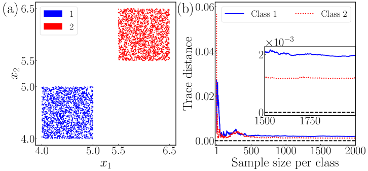
Figure 1: (a) A binary classification dataset. For class 1, features $x_{1}$ and $x_{2}$ obey the uniform distribution $\mathcal{U}[4,5]$, and for class 2, features $x_{1}$ and $x_{2}$ follow the uniform distribution $\mathcal{U}[5.5,6.5]$. Each class contains 2000 samples. (b) The trace distance between the averaged encoded states and the superposition state $\frac{1}{2}\mathbf{1}\mathbf{1}^{\top}$, where the solid blue line represents class 1 and the red dotted represents class 2.

Proposition 2.

Denote by $\mathcal{D}_{\mathcal{X}}$ the distribution of the feature $\boldsymbol{x}\in\mathbb{R}^{2^{n}}$. Assume that the elements of $\boldsymbol{x}$ are i.i.d with an expected value of $0$. In addition, the distribution is symmetric, i.e., $p(x_{j})=p(-x_{j})$ for all $j\in[0:2^{n}-1]$. Then after amplitude encoding, the expectation of encoded state is the maximally mixed state, i.e.,

$$\underset{\boldsymbol{x}\sim\mathcal{D}_{\mathcal{X}}}{\mathbb{E}}\left[\rho(\boldsymbol{x})\right]=\frac{\boldsymbol{I}}{2^{n}}.$$

Note that when the elements of the feature $\boldsymbol{x}$ are i.i.d., and symmetric about the mean value, to make the distribution satisfies the assumptions in Proposition 2, we can employ the standard $z$-score normalization Fei et al. (2021), namely, letting $z=\frac{x-\mu}{\sigma}$, where $\mu$ is the mean of $x$ and $\sigma$ is the standard variance.

We illustrate Proposition 2 by using a binary classification dataset in Fig. 2. It is clear that the features of class 1 and class 2 can be distinguished by their distances to the origin (or the $\ell_{2}$ norm). However, after amplitude encoding, their averaged encoded states concentrate to the maximally mixed state.

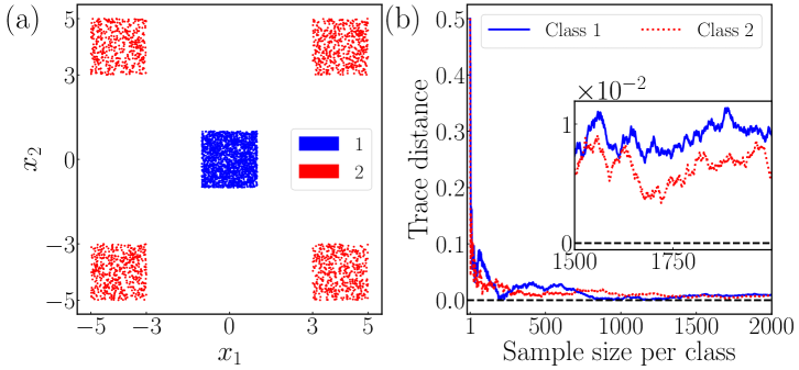
Figure 2: (a) A binary classification dataset. For class 1, features $x_{1}$ and $x_{2}$ obey the uniform distribution $\mathcal{U}[-1,1]$. For class 2, features $x_{1}$ and $x_{2}$ follow the uniform distribution over the intervals $[-5,-3]\cup[3,5]$. Each class contains 2000 samples. (b) The trace distance between the averaged encoded state and the maximally mixed state $\frac{\boldsymbol{I}}{2}$.

Proposition 3.

For a binary classification dataset, denote by $\mathcal{D}_{\mathcal{X}_{i}}$ the distribution of feature $\boldsymbol{x}\in\mathbb{R}^{2^{n}}$ in class $i$, $i=1,2$. If for any $j\in[0:2^{n}-1]$, the probability density functions $p_{i,j}(x)$ of the $j$-th element in class $i$ satisfy $p_{1,j}(x)=-p_{2,j}(x)$, then after amplitude encoding, the expected states of the two classes are identical, i.e.,

$$\underset{\boldsymbol{x}\sim\mathcal{D}_{\mathcal{X}_{1}}}{\mathbb{E}}\left[\rho(\boldsymbol{x})\right]=\underset{\boldsymbol{x}\sim\mathcal{D}_{\mathcal{X}_{2}}}{\mathbb{E}}\left[\rho(\boldsymbol{x})\right].$$

Proposition 3 indicates that the concentration phenomenon caused by amplitude encoding is not limited to convergence towards a specific state. We exemplify Proposition 3 in Fig. 3 by showing an example where the features of class 1 and class 2 are linearly separable, but the trace distance of their averaged encoded states converges to zero as the the sample size increases.

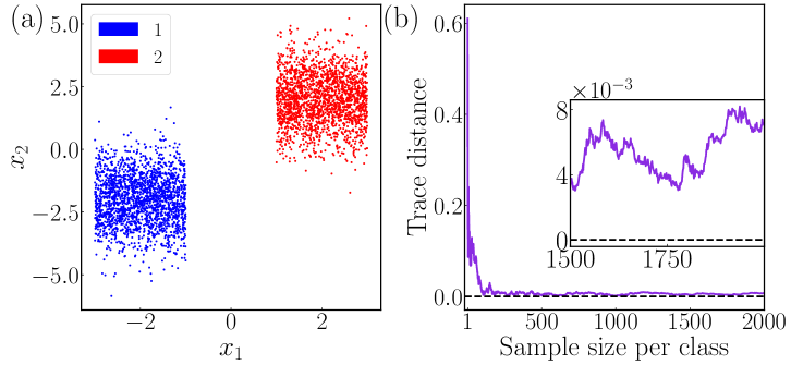
Figure 3: (a) A binary classification dataset. For class 1, $x_{1}$ follows the uniform distribution $\mathcal{U}[-3,-1]$, and $x_{2}$ follows the normal distribution $\mathcal{N}(-2,1)$. For class 2, $x_{1}$ obeys the uniform distribution $\mathcal{U}[1,3]$, and $x_{2}$ obeys the normal distribution $\mathcal{N}(2,1)$. Each class contains 2000 samples. (b) The trace distance between the averaged encoded states of class 1 and class 2.

The propositions in this subsection demonstrate that amplitude encoding may erase crucial information needed for classification, leading to the concentration phenomenon. This can result in poor performance of quantum classifiers. The detailed proofs of the propositions are provided in Appendix B.

III.3 Numerical validations

In this subsection, we verify the loss barrier phenomenon caused by amplitude encoding via numerical simulations.

To demonstrate the limitations of amplitude encoding, we examine the binary datasets depicted in Fig. 1(a) to Fig. 3(a). Under amplitude encoding, if even these simple binary datasets cannot be effectively categorized, it is unlikely that more complex datasets could be successfully classified. For these binary classifications tasks, we can just use a single qubit and employ a simple PQC, as illustrated in Fig. 4(a). The classical data are first encoded into quantum states via amplitude encoding. Then the quantum states pass through a total of $L$ layers, each of which comprises three quantum gates: $Rz$, $Rx$, and $Rz$, with independent parameters. The initial parameters are sampled from the standard normal distribution $\mathcal{N}(0,1)$. We train the variational parameters of the PQC by minimizing the loss function Eq. (2). For each dataset, we choose the Pauli Z as the observable for class 1 and the Pauli X as the observable for class 2. We utilize the Adam optimizer with a learning rate of 0.01 for the training.

We conduct numerical simulations for three scenarios with $L=1$, $L=10$, and $L=30$, respectively. Each scenario is repeated 10 rounds, with random initializations of the circuit parameters and 1000 iterations per round. Fig 4.(b) displays the training loss for the datasets from Fig. 1(a), Fig. 2(a), and Fig. 3(a) with $L=10$. It is clear that at the initial stage of training, there is a significant descent in the loss function value, indicating that the gradient of the loss function does not vanish at the beginning of training. However, the loss function quickly converges to around $\ln 2$, demonstrating the loss barrier phenomenon. Similar results are observed for $L=1$ and $L=30$, and the details are presented in Appendix C.

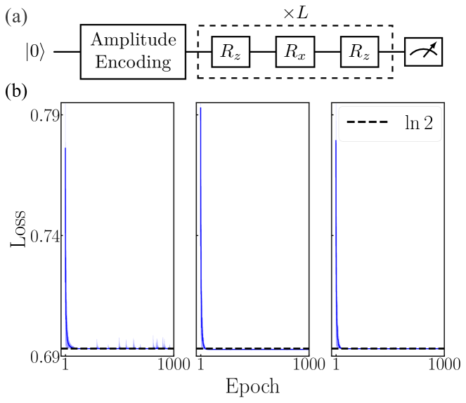
Figure 4: (a) The PQC with $L$ layers used for quantum binary classification. (b) Training loss for datasets from Fig. 1(a), Fig. 2(a), and Fig. 3(a) (from left to right). Blue solid lines depict the mean loss over 10 runs, and the shaded areas show their range.

To further demonstrate the negative impact of loss barrier, we present in Table 1 the best training accuracy obtained within 1000 iterations for the three datasets. We find that the best training accuracy is around 0.5 with a relatively small standard deviation. This implies that, owing to the presence of loss barrier phenomenon, it is impossible to train a quantum classifier with satisfactory performance. The essential reason is the concentration phenomenon induced by amplitude encoding.

Table 1: Best training accuracy for datasets from Fig. 1(a) to Fig. 3(a). The values in the table represent the mean $\pm$ standard deviation over 10 runs.

	Fig. 1(a)	Fig. 2(a)	Fig. 3(a)
Accuracy	0.534 $\pm$ 0.001	0.517 $\pm$ 0.000	0.511 $\pm$ 0.001

III.4 Real-world datasets scenario

In this subsection, we consider real-world datasets and demonstrate that the concentration phenomenon induced by amplitude encoding is widespread.

We select common computer vision datasets for classification, including forests and sea lakes from the EuroSAT dataset ($64\times 64$ pixels) Helber et al. (2019), adipose tissues and backgrounds from the PathMNIST dataset ($28\times 28$ pixels) Yang et al. (2023), and airplanes and birds from the CIFAR-10 dataset ($32\times 32$ pixels) Krizhevsky (2009). We label these pairs as class 1 and class 2, respectively, and compute the trace distance between the averaged encoded states of the two classes. For comparison, we also consider the MNIST dataset and take digits 0 and 1 ($28\times 28$ pixels) to be class 1 and class 2 LeCun , which are frequently used in quantum classification tasks LaRose and Coyle (2020); Grant et al. (2018); Hur et al. (2022); Mitsuda et al. (2024); Wang et al. (2024a); Li et al. (2024). For all datasets, we resize the images to $32\times 32$ pixels and employ 10 qubits for amplitude encoding.

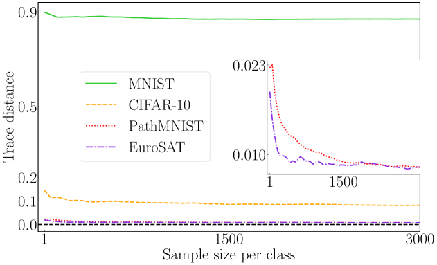
Figure 5: The trace distance between the averaged encoded states of class 1 and class 2 for different datasets.

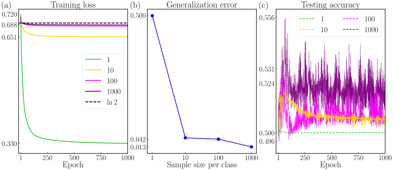
Figure 6: Quantum classification performance for EuroSAT dataset. (a) The average training loss of the quantum classifier over 10 runs for different sample sizes per class. (b) The average generalization error over 10 runs with 1000 iterations of each run (10000 results in total) versus different sample sizes per class. (c) The average testing accuracy obtained over 10 runs for different sample sizes per class.

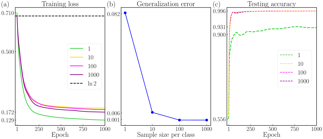
Figure 7: Quantum classification performance for MNIST dataset. (a) The average training loss over 10 runs for different sample sizes per class. (b) The average generalization error over 10 runs versus different sample sizes per class. (c) The average testing accuracy over 10 runs for different sample sizes per class.

As illustrated in Fig. 5, the trace distances between the averaged encoded states of the respective two classes in the EuroSAT, PathMNIST, and CIFAR-10 datasets consistently remain below 0.2 as the sample size increases. Notably, for the EuroSAT and PathMNIST datasets, the trace distances are even less than 0.023. In contrast, for the relatively simple and sparse MNIST dataset, the trace distance between the averaged encoded states of the two classes is close to 0.9. The comparisons in Fig. 5 imply that good performance of quantum classifiers under amplitude encoding on the MNIST dataset may not be generalized to more complex datasets.

To see this, we employ the quantum convolutional neural network (QCNN) as the PQC to train a quantum classifier to categorize the EuroSAT dataset. The QCNN has been shown to be free from barren plateaus Pesah et al. (2021), and has been widely used for quantum classification tasks. We illustrate the QCNN circuit in Appendix D. Similar to Sec. III.3, we employ the Adam as the optimizer with a learning rate of 0.01. For class 1, we use the Pauli Z operator on the first qubit as the observable, while for class 2, we use the Pauli X operator on the first qubit as the observable. We ensure that the two classes have the same number of samples. We conduct simulations for 10 rounds, and in each round the parameters of the QCNN are independently initialized following the standard normal distribution $\mathcal{N}(0,1)$. After training, we employ a test set consisting of 4000 new, unseen samples (2000 per class), and calculate the accuracy on this test set as the prediction accuracy.

We depict the performance of the trained quantum classifier in Fig. 6. From Fig. 6(a), as the sample size increases, the average convergence value of its training loss increases and approaches to $\ln 2$. Fig. 6(b) illustrates the average of the generalization error (Eq. (3)) over 10 runs with 1000 iterations of each run (10000 results in total). We find that the generalization error decreases as the sample size increases. From Fig. 6(c), we find that for different sample sizes, the average prediction accuracy remains around 0.5 and never exceeds 0.56, indicating poor classification performance on the EuroSAT dataset under amplitude encoding.

Then for comparison, we also perform numerical simulations on the MNIST dataset under the same settings as those for the EuroSAT dataset, including the circuit, optimizer, learning rate, parameter initializations, and observables. We demonstrate the results in Fig. 7. Notably, the training losses on the MNIST dataset are significantly lower than ln2 across different sample sizes, which is in stark contrast to the EuroSAT dataset case. Most remarkably, a prediction accuracy above 0.9 can be achieved with just one sample per class, and when the number of samples per class exceeds 10, the testing accuracy remains consistently above 0.99. The success of classification under amplitude encoding on the MNIST dataset can be attributed to the sparsity of its features. The comparison between the MNIST and EuroSAT datasets indicates that findings validated on the MNIST dataset may not be readily generalized to more complex, real-world datasets.

IV Conclusion

We have investigated the concentration phenomenon induced by amplitude encoding and the resulting loss barrier phenomenon. Since encoding is a necessary and crucial step in leveraging QML to address classical problems, our findings indicate that the direct use of amplitude encoding may undermine the potential advantages of QML. Therefore, more effort should be devoted to developing more efficient encoding strategies to fully unlock the potential of QML.

Appendix A Proof of Theorem 1

Theorem A.1 (Theorem 1 in the main text).

For a $K$-class classification, we employ the cross-entropy loss function $\mathcal{L}_{S}(\boldsymbol{\theta})$ defined in Eq. (2). The quantum classifier is trained on a balanced training set $S=\{(\boldsymbol{x}^{(m)},y^{(m)})\}_{m=1}^{M}$, where each class contains $M/K$ samples. Suppose the eigenvalues of each observable $H_{k}$ belong to $[-1,1]$, for $k=1,\ldots,K$. If the trace distance between the expectations of encoded states of any different classes is less than $\epsilon$, then for any PQC $U(\boldsymbol{\theta})$ and optimization algorithm, we have

$$\mathcal{L}_{S}(\boldsymbol{\theta})\geqslant\ln\left[K-4(K-1)\epsilon\right]$$ (7)

with probability at least $1-8e^{-M\epsilon^{2}/8K}$.

Proof.

For the training set $S$, we denote by $\boldsymbol{x}^{(k,m)}$ the $m$-th feature of the $k$-th class, and $\boldsymbol{x}^{(j,n)}$ the $n$-th feature of the $j$-th class. For the observable $H_{l}$, the corresponding expectations of measurements read

$$h_{l}^{(k,m)} \coloneqq\operatorname{Tr}\left[H_{l}U(\boldsymbol{\theta})\rho(\boldsymbol{x}^{(k,m)})U^{\dagger}\left(\boldsymbol{\theta}\right)\right],$$

$$h_{l}^{(j,n)} \coloneqq\operatorname{Tr}\left[H_{l}U\left(\boldsymbol{\theta}\right)\rho(\boldsymbol{x}^{(j,n)})U^{\dagger}(\boldsymbol{\theta})\right].$$

According to the assumption, the training set $S$ contains $M$ samples in total, with $M^{\prime}=M/K$ samples per class. For the $k$-th class, we define the averaged expectation value over the subset of training samples $\{(\boldsymbol{x}^{(k,m)},k)\}_{m=1}^{M^{\prime}}$ as $\overline{h}_{l}^{(k)}\coloneqq\frac{1}{M^{\prime}}\sum_{m=1}^{M^{\prime}}h_{l}^{(k,m)}$. Similarly, we define the averaged encoded state $\overline{\rho}_{M^{\prime}}^{(k)}\coloneqq\frac{1}{M^{\prime}}\sum_{m=1}^{M^{\prime}}\rho(\boldsymbol{x}^{(k,m)})$ for this subset. For the $j$-th class, we define $\overline{h}_{l}^{(j)}\coloneqq\frac{1}{M^{\prime}}\sum_{n=1}^{M^{\prime}}h_{l}^{(j,n)}$ and $\overline{\rho}_{M^{\prime}}^{(j)}\coloneqq\frac{1}{M^{\prime}}\sum_{n=1}^{M^{\prime}}\rho(\boldsymbol{x}^{(j,n)})$, in a similar manner.

By applying Hölder’s inequality, we have

$$\left|\overline{h}_{l}^{(k)}-\overline{h}_{l}^{(j)}\right| =\left|\operatorname{Tr}\left[H_{l}U(\boldsymbol{\theta})\left(\overline{\rho}_{M^{\prime}}^{(k)}-\overline{\rho}_{M^{\prime}}^{(j)}\right)U^{\dagger}(\boldsymbol{\theta})\right]\right|$$

$$\leqslant\Big{\|}U^{\dagger}(\boldsymbol{\theta})H_{l}U(\boldsymbol{\theta})\Big{\|}_{\infty}\left\|\overline{\rho}_{M^{\prime}}^{(k)}-\overline{\rho}_{M^{\prime}}^{(j)}\right\|_{1}$$

$$\leqslant\left\|\overline{\rho}_{M^{\prime}}^{(k)}-\underset{\boldsymbol{x}^{(k)}\sim\mathcal{D}_{\mathcal{X}_{k}}}{\mathbb{E}}[\rho(\boldsymbol{x}^{(k)})]+\underset{\boldsymbol{x}^{(k)}\sim\mathcal{D}_{\mathcal{X}_{k}}}{\mathbb{E}}[\rho(\boldsymbol{x}^{(k)})]-\overline{\rho}_{M^{\prime}}^{(j)}\right\|_{1}$$

$$\leqslant\left\|\overline{\rho}_{M^{\prime}}^{(k)}-\underset{\boldsymbol{x}^{(k)}\sim\mathcal{D}_{\mathcal{X}_{k}}}{\mathbb{E}}[\rho(\boldsymbol{x}^{(k)})]\right\|_{1}+\left\|\underset{\boldsymbol{x}^{(k)}\sim\mathcal{D}_{\mathcal{X}_{k}}}{\mathbb{E}}[\rho(\boldsymbol{x}^{(k)})]-\overline{\rho}_{M^{\prime}}^{(j)}\right\|_{1}$$

$$\leqslant\left\|\overline{\rho}_{M^{\prime}}^{(k)}-\underset{\boldsymbol{x}^{(k)}\sim\mathcal{D}_{\mathcal{X}_{k}}}{\mathbb{E}}[\rho(\boldsymbol{x}^{(k)})]\right\|_{1}+\left\|\underset{\boldsymbol{x}^{(k)}\sim\mathcal{D}_{\mathcal{X}_{k}}}{\mathbb{E}}[\rho(\boldsymbol{x}^{(k)})]-\underset{\boldsymbol{x}^{(j)}\sim\mathcal{D}_{\mathcal{X}_{j}}}{\mathbb{E}}[\rho(\boldsymbol{x}^{(j)})]+\underset{\boldsymbol{x}^{(j)}\sim\mathcal{D}_{\mathcal{X}_{j}}}{\mathbb{E}}[\rho(\boldsymbol{x}^{(j)})]-\overline{\rho}_{M^{\prime}}^{(j)}\right\|_{1}$$

$$\leqslant\left\|\overline{\rho}_{M^{\prime}}^{(k)}-\underset{\boldsymbol{x}^{(k)}\sim\mathcal{D}_{\mathcal{X}_{k}}}{\mathbb{E}}[\rho(\boldsymbol{x}^{(k)})]\right\|_{1}+\left\|\underset{\boldsymbol{x}^{(k)}\sim\mathcal{D}_{\mathcal{X}_{k}}}{\mathbb{E}}[\rho(\boldsymbol{x}^{(k)})]-\underset{\boldsymbol{x}^{(j)}\sim\mathcal{D}_{\mathcal{X}_{j}}}{\mathbb{E}}[\rho(\boldsymbol{x}^{(j)})]\right\|_{1}+\left\|\underset{\boldsymbol{x}^{(j)}\sim\mathcal{D}_{\mathcal{X}_{j}}}{\mathbb{E}}[\rho(\boldsymbol{x}^{(j)})]-\overline{\rho}_{M^{\prime}}^{(j)}\right\|_{1}.$$

According to Lemma 1, it yields

$$\left\|\overline{\rho}_{M^{\prime}}^{(k)}-\underset{\boldsymbol{x}^{(k)}\sim\mathcal{D}_{\mathcal{X}_{k}}}{\mathbb{E}}[\rho(\boldsymbol{x}^{(k)})]\right\|_{1}+\left\|\underset{\boldsymbol{x}^{(j)}\sim\mathcal{D}_{\mathcal{X}_{j}}}{\mathbb{E}}[\rho(\boldsymbol{x}^{(j)})]-\overline{\rho}_{M^{\prime}}^{(j)}\right\|_{1}\leqslant 2\epsilon,$$

with probability at least $1-8e^{-M^{\prime}\epsilon^{2}/8}$. Combining this with our assumption that

$$\left\|\underset{\boldsymbol{x}^{(k)}\sim\mathcal{D}_{\mathcal{X}_{k}}}{\mathbb{E}}[\rho(\boldsymbol{x}^{(k)})]-\underset{\boldsymbol{x}^{(j)}\sim\mathcal{D}_{\mathcal{X}_{j}}}{\mathbb{E}}[\rho(\boldsymbol{x}^{(j)})]\right\|_{1}\leqslant 2\epsilon,$$

we have

$$\left|\overline{h}_{l}^{(k)}-\overline{h}_{l}^{(j)}\right| =\left|\operatorname{Tr}\left[H_{l}U(\boldsymbol{\theta})\left(\overline{\rho}_{M^{\prime}}^{(k)}-\overline{\rho}_{M^{\prime}}^{(j)}\right)U^{\dagger}(\boldsymbol{\theta})\right]\right|\leqslant 4\epsilon,$$ (8)

with probability at least $1-8e^{-M\epsilon^{2}/8K}$.

We now derive the lower bound for the cross-entropy function. According to Eq. (2), the cross-entropy reads

$$\mathcal{L}_{S}(\boldsymbol{\theta}) =\frac{1}{M}\sum_{m=1}^{M}\ell(\boldsymbol{\theta};\boldsymbol{x}^{(m)},y^{(m)})$$

$$=-\frac{1}{M}\sum_{m=1}^{M}\sum_{k=1}^{K}\boldsymbol{y}_{k}^{(m)}\ln\left(\frac{\mathrm{e}^{h_{k}(\boldsymbol{x}^{(m)},\boldsymbol{\theta})}}{\sum_{j=1}^{K}\mathrm{e}^{h_{j}(\boldsymbol{x}^{(m)},\boldsymbol{\theta})}}\right)$$

$$=\frac{1}{M}\sum_{m=1}^{M}\sum_{k=1}^{K}\boldsymbol{y}_{k}^{(m)}\ln\left(\frac{\sum_{j=1}^{K}\mathrm{e}^{h_{j}(\boldsymbol{x}^{(m)},\boldsymbol{\theta})}}{\mathrm{e}^{h_{k}(\boldsymbol{x}^{(m)},\boldsymbol{\theta})}}\right)$$

$$=\frac{1}{M}\sum_{m=1}^{M}\sum_{k=1}^{K}\boldsymbol{y}_{k}^{(m)}\ln\left[\sum_{j=1}^{K}\exp\left\{h_{j}(\boldsymbol{x}^{(m)},\boldsymbol{\theta})-h_{k}(\boldsymbol{x}^{(m)},\boldsymbol{\theta})\right\}\right]$$

$$=\frac{1}{K}\sum_{k=1}^{K}\frac{1}{M^{\prime}}\sum_{m=1}^{M^{\prime}}\ln\left[\sum_{j=1}^{K}\exp\left\{h_{j}(\boldsymbol{x}^{(k,m)},\boldsymbol{\theta})-h_{k}(\boldsymbol{x}^{(k,m)},\boldsymbol{\theta})\right\}\right],$$ (9)

where Eq. (9) arises from the fact that only the feature $\boldsymbol{x}^{(m)}$ from the $k$-th class has $\boldsymbol{y}_{k}^{(m)}\neq 0$, and in this case, $\boldsymbol{y}_{k}^{(m)}=1$.

We then apply Jensen’s inequality to the convex function $\ln[\sum_{j=1}^{K}e^{x_{j}}]$ on $\mathbb{R}^{K}$ Boyd and Vandenberghe (2004). It yields

$$\mathcal{L}_{S}(\boldsymbol{\theta}) =\frac{1}{K}\sum_{k=1}^{K}\frac{1}{M^{\prime}}\sum_{m=1}^{M^{\prime}}\ln\left[\sum_{j=1}^{K}\exp\left\{h_{j}^{(k,m)}-h_{k}^{(k,m)}\right\}\right]$$

$$\geqslant\frac{1}{K}\sum_{k=1}^{K}\ln\left[\sum_{j=1}^{K}\exp\left\{\frac{1}{M^{\prime}}\sum_{m=1}^{M^{\prime}}\left(h_{j}^{(k,m)}-h_{k}^{(k,m)}\right)\right\}\right]$$ (10)

$$=\frac{1}{K}\sum_{k=1}^{K}\ln\left[\sum_{j=1}^{K}\exp\left\{\overline{h}_{j}^{(k)}-\overline{h}_{k}^{(k)}\right\}\right]$$

$$\geqslant\ln\left[\sum_{j=1}^{K}\exp\left\{\frac{1}{K}\sum_{k=1}^{K}\left(\overline{h}_{j}^{(k)}-\overline{h}_{k}^{(k)}\right)\right\}\right]$$ (11)

$$\geqslant\ln\left[\sum_{j=1}^{K}\left\{\frac{1}{K}\sum_{k=1}^{K}\left(\overline{h}_{j}^{(k)}-\overline{h}_{k}^{(k)}\right)+1\right\}\right]$$ (12)

$$=\ln\left[\frac{1}{K}\sum_{j=1}^{K}\sum_{k=1}^{K}\left(\overline{h}_{j}^{(k)}-\overline{h}_{k}^{(k)}\right)+K\right],$$ (13)

where inequalities (10) and (11) are derived from Jensen’s inequality, and inequality (12) follows from the inequality $e^{x}\geqslant x+1$.

Since Eq. (13) involves a double summation over indices $j$ and $k$, we can change the subscripts of $h_{k}^{(k)}$ to $h_{j}^{(j)}$. This yields

$$\mathcal{L}_{S}(\boldsymbol{\theta}) \geqslant\ln\left[\frac{1}{K}\sum_{j=1}^{K}\sum_{k=1}^{K}\left(\overline{h}_{j}^{(k)}-\overline{h}_{k}^{(k)}\right)+K\right]$$

$$=\ln\left[\frac{1}{K}\sum_{k=1}^{K}\sum_{j=1}^{K}\left(\overline{h}_{j}^{(k)}-\overline{h}_{j}^{(j)}\right)+K\right].$$

Finally, combining this with Eq. (8), we have

$$\mathcal{L}_{S}(\boldsymbol{\theta}) \geqslant\ln\left[K-4(K-1)\epsilon\right]$$

with probability at least $1-8e^{-M\epsilon^{2}/8K}$. ∎

Appendix B Proofs of concentrations

Lemma B.1 (Lemma 1 in the main text).

Given an arbitrary $\epsilon\in(0,1)$, we have

$$T\left(\overline{\rho}_{M},\mathbb{E}[\rho]\right)\leq\epsilon$$

with probability at least $1-4e^{-M\epsilon^{2}/2}$.

Proof.

For any linear operator $X$ defined on a linear space $\mathcal{X}$, its Schatten-1 norm reads

$$\left\|X\right\|_{1}=\max_{U\in\mathrm{U}(\mathcal{X})}|\langle U,X\rangle|,$$

where $\mathrm{U}(\mathcal{X})$ denotes the set of unitary operators on space $\mathcal{X}$. Consequently, we can express

$$\left\|\bar{\rho}_{M}-\mathbb{E}[\rho]\right\|_{1}=\max_{U\in\mathrm{U}(\mathcal{X})}|\langle U,\bar{\rho}_{M}-\mathbb{E}[\rho]\rangle|,$$

and

$$|\langle U,\bar{\rho}_{M}-\mathbb{E}[\rho]\rangle|=|\mathrm{Tr}\left[U^{\dagger}(\bar{\rho}_{M}-\mathbb{E}[\rho])\right]|=|\mathrm{Tr}\left[U^{\dagger}\bar{\rho}_{M}\right]-\mathrm{Tr}\left[U^{\dagger}\mathbb{E}[\rho]\right]|.$$

The complex-valued term $\mathrm{Tr}\left[U^{\dagger}\bar{\rho}_{M}\right]$ can be decomposed into its real and imaginary components as

$$\mathrm{Tr}\left[U^{\dagger}\bar{\rho}_{M}\right]=\mathrm{Re}\{\mathrm{Tr}\left[U^{\dagger}\bar{\rho}_{M}\right]\}+\mathrm{i}\,\mathrm{Im}\{\mathrm{Tr}\left[U^{\dagger}\bar{\rho}_{M}\right]\}.$$

For the real component, we have

$$\mathrm{Re}\{\mathrm{Tr}\left[U^{\dagger}\bar{\rho}_{M}\right]\}=\frac{1}{M}\sum_{m=1}^{M}\mathrm{Re}\left\{\mathrm{Tr}\left[U^{\dagger}\rho(\boldsymbol{x}^{(m)})\right]\right\}.$$

Given that $\left|\mathrm{Tr}\left[U^{\dagger}\bar{\rho}_{M}\right]\right|\leq\|U^{\dagger}\|_{\infty}\|\rho\|_{1}=1$, and considering that for any complex number $z=a+\mathrm{i}b$, $|z|=\sqrt{a^{2}+b^{2}}\geq|a|$, we can see that $\frac{1}{M}\mathrm{Re}\left\{\mathrm{Tr}\left[U^{\dagger}\rho(\boldsymbol{x}^{(m)})\right]\right\}$ is an independent random variable bounded within $\left[-\frac{1}{M},\frac{1}{M}\right]$. Applying Hoeffding’s inequality Mohri et al. (2018) yields

$$\left|\frac{1}{M}\sum_{m=1}^{M}\mathrm{Re}\left\{\mathrm{Tr}\left[U^{\dagger}\rho(\boldsymbol{x}^{(m)})\right]\right\}-\underset{\boldsymbol{x}\sim\mathcal{D}_{\mathcal{X}}}{\mathbb{E}}\left(\mathrm{Re}\left\{\mathrm{Tr}\left[U^{\dagger}\rho(\boldsymbol{x})\right]\right\}\right)\right|\leq\epsilon,$$

with probability at least $1-2e^{-M\epsilon^{2}/2}$.

By the definitions of $\bar{\rho}_{M}$ and $\mathbb{E}[\rho]$, we obtain $\left|\mathrm{Re}\left\{\mathrm{Tr}\left[U^{\dagger}\bar{\rho}_{M}\right]-\mathrm{Tr}\left[U^{\dagger}\mathbb{E}[\rho]\right]\right\}\right|\leq\epsilon$ with probability at least $1-2e^{-M\epsilon^{2}/2}$. Following a similar argument, we have $\left|\mathrm{Im}\left\{\mathrm{Tr}\left[U^{\dagger}\bar{\rho}_{M}\right]-\mathrm{Tr}\left[U^{\dagger}\mathbb{E}[\rho]\right]\right\}\right|\leq\epsilon$ with the same probability at least $1-2e^{-M\epsilon^{2}/2}$.

Therefore, by the triangle inequality, we have

$$\left|\mathrm{Tr}\left[U^{\dagger}\bar{\rho}_{M}\right]-\mathrm{Tr}\left[U^{\dagger}\mathbb{E}[\rho]\right]\right| =\left|\mathrm{Re}\left\{\mathrm{Tr}\left[U^{\dagger}\bar{\rho}_{M}\right]-\mathrm{Tr}\left[U^{\dagger}\mathbb{E}[\rho]\right]\right\}+\mathrm{i}\,\mathrm{Im}\left\{\mathrm{Tr}\left[U^{\dagger}\bar{\rho}_{M}\right]-\mathrm{Tr}\left[U^{\dagger}\mathbb{E}[\rho]\right]\right\}\right|$$

$$\leq\left|\mathrm{Re}\left\{\mathrm{Tr}\left[U^{\dagger}\bar{\rho}_{M}\right]-\mathrm{Tr}\left[U^{\dagger}\mathbb{E}[\rho]\right]\right\}\right|+\left|\mathrm{Im}\left\{\mathrm{Tr}\left[U^{\dagger}\bar{\rho}_{M}\right]-\mathrm{Tr}\left[U^{\dagger}\mathbb{E}[\rho]\right]\right\}\right|$$

$$\leq 2\epsilon,$$

with probability at least $1-4e^{-M\epsilon^{2}/2}$. Finally, we can conclude that

$$T(\bar{\rho}_{M},\mathbb{E}[\rho])=\frac{1}{2}\left\|\bar{\rho}_{M}-\mathbb{E}[\rho]\right\|_{1}=\frac{1}{2}\max_{U\in\mathrm{U}(\mathcal{X})}\left|\langle U,\bar{\rho}_{M}-\mathbb{E}[\rho]\rangle\right|\leq\epsilon,$$

with probability at least $1-4e^{-M\epsilon^{2}/2}$.

∎

Proposition B.1 (Proposition 1 in the main text).

Assume that all elements in the feature $\boldsymbol{x}\in\mathbb{R}^{2^{n}}$ have the same sign, and the elements satisfy $|x_{i}|\in[m,M]$. If $\left|\frac{m}{M}-1\right|<\epsilon$, then after amplitude encoding, we have

$$T\left(\rho(\boldsymbol{x}),\frac{1}{2^{n}}\mathbf{1}\mathbf{1}^{\top}\right)\leqslant\sqrt{2\epsilon},$$

where the state $\frac{1}{2^{n}}\boldsymbol{1}\boldsymbol{1}^{\top}=|+\rangle_{n}\langle+|_{n}$, with $|+\rangle_{n}=H^{\otimes n}|0\rangle_{n}$ being the superposition of all computational basis states.

Proof.

For the feature vector $\boldsymbol{x}=[x_{0},x_{1},\cdots,x_{2^{n}-1}]^{\top}$, denote that the encoded state vector as $|\psi(\boldsymbol{x})\rangle$, with the density matrix as $\rho(\boldsymbol{x})$. Then, the probability amplitude of the encoded state correspondingto the basis vector $|i\rangle$ reads

$$\alpha_{i}=\sqrt{\frac{x_{i}^{2}}{x_{0}^{2}+x_{1}^{2}+\cdots x_{2^{n}-1}^{2}}}.$$

The corresponding probability of projection into the basis vector $|i\rangle$ is

$$p_{i}=|\alpha_{i}|^{2}=\frac{x_{i}^{2}}{x_{0}^{2}+x_{1}^{2}+\cdots x_{2^{n}-1}^{2}}=\frac{1}{1+(x_{0}/x_{i})^{2}+\cdots+(x_{2^{n}-1}/x_{i})^{2}}.$$

If $|x_{i}|\in[m,M]$, then

$$p_{i}=\frac{1}{1+(x_{0}/x_{i})^{2}+\cdots+(x_{2^{n}-1}/x_{i})^{2}}\geqslant\frac{1}{1+(2^{n}-1)(M/m)^{2}}.$$

Let $x=\frac{m}{M}$, where $x\in(0,1]$, and define $f_{\min}(x)=\frac{x^{2}}{x^{2}+(2^{n}-1)}$. Thus, we have

$$\left|2^{n}f_{\min}(x)-1\right| =\left|\frac{2^{n}x^{2}-x^{2}-(2^{n}-1)}{x^{2}+(2^{n}-1)}\right|$$

$$=\left|\frac{(2^{n}-1)(x^{2}-1)}{x^{2}+(2^{n}-1)}\right|$$

$$\leqslant|x^{2}-1|$$

$$\leqslant 2\epsilon.$$

Thus, $f_{\min}(\frac{m}{M})=\frac{1}{1+(2^{n}-1)(M/m)^{2}}\geqslant\frac{1}{2^{n}}\cdot(1-2\epsilon).$

The absolute value of the inner product between the encoded state vector $|\psi(\boldsymbol{x})\rangle$ and the $n$-qubit superposition state $|+\rangle_{n}$ satisfies

$$\Big{|}\langle\psi(\boldsymbol{x})|+\rangle_{n}\Big{|} =\left|\sum_{i=0}^{2^{n}-1}\frac{1}{\sqrt{2^{n}}}\frac{x_{i}}{\sqrt{x_{0}^{2}+\cdots+x_{2^{n}-1}}}\right|$$

$$=\frac{1}{\sqrt{2^{n}}}\sum_{i=0}^{2^{n}-1}\left|\frac{x_{i}}{\sqrt{x_{0}^{2}+\cdots+x_{2^{n}-1}^{2}}}\right|$$

$$=\frac{1}{\sqrt{2^{n}}}\sum_{i=0}^{2^{n}-1}\sqrt{\frac{1}{1+(x_{0}/x_{i})^{2}+\cdots+(x_{2^{n}-1}/x_{i})^{2}}}$$

$$\geqslant\frac{1}{\sqrt{2^{n}}}\sum_{i=0}^{2^{n}-1}\sqrt{\frac{1}{1+(2^{n}-1)(M/m)^{2}}}$$

$$\geqslant\sum_{i=0}^{2^{n}-1}\frac{1}{\sqrt{2^{n}}}\cdot\frac{1}{\sqrt{2^{n}}}\cdot\sqrt{1-2\epsilon}$$

$$\geqslant\sqrt{1-2\epsilon}.$$

Since both the encoded state $|\psi(\boldsymbol{x})\rangle$ and the superposition state $|+\rangle_{n}$ are pure, we have

$$T\left(\rho(\boldsymbol{x}),\frac{1}{2^{n}}\mathbf{1}\mathbf{1}^{\top}\right)=\frac{1}{2}\left\|\rho(\boldsymbol{x})-\frac{1}{2^{n}}\mathbf{1}\mathbf{1}^{\top}\right\|_{1} =\sqrt{1-|\langle\psi(\boldsymbol{x})|+\rangle_{n}|^{2}}\leqslant\sqrt{2\epsilon}.$$

∎

Proposition B.2 (Proposition 2 in the main text).

Denote by $\mathcal{D}_{\mathcal{X}}$ the distribution of the feature $\boldsymbol{x}\in\mathbb{R}^{2^{n}}$. Assume that the elements of $\boldsymbol{x}$ are i.i.d with an expected value of $0$. In addition, the distribution is symmetric, i.e., $p(x_{j})=p(-x_{j})$, for all $j\in[0:2^{n}-1]$. Then after amplitude encoding, the expectation of encoded state is the maximally mixed state, i.e.,

$$\underset{\boldsymbol{x}\sim\mathcal{D}_{\mathcal{X}}}{\mathbb{E}}\left[\rho(\boldsymbol{x})\right]=\frac{\boldsymbol{I}}{2^{n}}.$$

Proof.

For the feature vector $\boldsymbol{x}=[x_{0},x_{1},\cdots,x_{2^{n}-1}]^{\top}$, according to the definition of amplitude encoding in Eq. (1), the expectation of encoded states reads

$$\underset{\boldsymbol{x}\sim\mathcal{D}_{\mathcal{X}}}{\mathbb{E}}\left[\rho(\boldsymbol{x})\right] =\underset{\boldsymbol{x}\sim\mathcal{D}_{\mathcal{X}}}{\mathbb{E}}\left(\sum_{i=0}^{2^{n}-1}\sum_{i=0}^{2^{n}-1}\frac{x_{i}x_{j}}{C_{\boldsymbol{x}}^{2}}|i\rangle\langle j|\right)$$

$$=\sum_{i=0}^{2^{n}-1}\sum_{j=0}^{2^{n}-1}\underset{\boldsymbol{x}\sim\mathcal{D}_{\mathcal{X}}}{\mathbb{E}}\left(\frac{x_{i}x_{j}}{x_{0}^{2}++\cdots+x_{2^{n}-1}^{2}}\right)|i\rangle\langle j|.$$

(1) Consider the diagonal elements:

$$\underset{\boldsymbol{x}\sim\mathcal{D}_{\mathcal{X}}}{\mathbb{E}}\left(\frac{x_{i}^{2}}{x_{0}^{2}++\cdots+x_{2^{n}-1}^{2}}\right) =\underset{\boldsymbol{x}\sim\mathcal{D}_{\mathcal{X}}}{\mathbb{E}}\left(1\right)-\underset{\boldsymbol{x}\sim\mathcal{D}_{\mathcal{X}}}{\mathbb{E}}\left(\frac{x_{0}^{2}+\cdots+x_{i-1}^{2}+x_{i+1}^{2}+\cdots+x_{2^{n}-1}^{2}}{x_{0}^{2}+\cdots+x_{2^{n}-1}^{2}}\right)$$

$$=1-\sum_{j=0,j\neq i}^{2^{n}-1}\underset{\boldsymbol{x}\sim\mathcal{D}_{\mathcal{X}}}{\mathbb{E}}\left(\frac{x_{j}^{2}}{x_{0}^{2}+\cdots+x_{2^{n}-1}^{2}}\right).$$

Note that the elements $x_{j}$s’ are independent and identically distributed. We assume that $\mathbb{E}_{\boldsymbol{x}\sim\mathcal{D}_{\mathcal{X}}}\left(\frac{x_{j}^{2}}{x_{0}^{2}+\cdots+x_{2^{n}-1}^{2}}\right)=a$. Then we have $a=1-(2^{n}-1)a$, and $a=\frac{1}{2^{n}}$, accordingly. Thus, for all diagonal elements, we have $\mathbb{E}_{\boldsymbol{x}\sim\mathcal{D}_{\mathcal{X}}}\left(\frac{x_{i}^{2}}{C_{\boldsymbol{x}}^{2}}\right)=\frac{1}{2^{n}}$.

(2) Consider the non-diagonal elements:

$$\underset{\boldsymbol{x}\sim\mathcal{D}_{\mathcal{X}}}{\mathbb{E}}\left(\frac{x_{i}x_{j}}{C_{\boldsymbol{x}}^{2}}\right) =\underset{\boldsymbol{x}\sim\mathcal{D}_{\mathcal{X}}}{\mathbb{E}}\left(\frac{x_{i}x_{j}}{x_{0}^{2}+\cdots+x_{2^{n}-1}^{2}}\right).$$

Since $\frac{(-x_{i})x_{j}}{x_{0}^{2}+\cdots+x_{2^{n}-1}^{2}}=-\frac{x_{i}x_{j}}{x_{0}^{2}+\cdots+x_{2^{n}-1}^{2}}$, and the distribution of $x_{j}$ is symmetric, we have

$$\underset{\boldsymbol{x}\sim\mathcal{D}_{\mathcal{X}}}{\mathbb{E}}\left(\frac{x_{i}x_{j}}{C_{\boldsymbol{x}}^{2}}\right) =\underset{\boldsymbol{x}\sim\mathcal{D}_{\mathcal{X}}}{\mathbb{E}}\left(\frac{x_{i}x_{j}}{x_{0}^{2}+\cdots+x_{2^{n}-1}^{2}}\right)=0.$$

Therefore,

$$\underset{\boldsymbol{x}\sim\mathcal{D}_{\mathcal{X}}}{\mathbb{E}}\left(\frac{x_{i}x_{j}}{C_{\boldsymbol{x}}^{2}}\right)=\begin{cases}\frac{1}{2^{n}}&i=j;\\ 0&i\neq j.\end{cases}$$

This implies that the expectation of encoded states is the maximally mixed state, i.e., $\underset{\boldsymbol{x}\sim\mathcal{D}_{\mathcal{X}}}{\mathbb{E}}\left[\rho(\boldsymbol{x})\right]=\frac{I}{2^{n}}$. ∎

Proposition B.3 (Proposition 3 in the main text).

For a binary classification dataset, denote by $\mathcal{D}_{\mathcal{X}_{i}}$ the distribution of feature $\boldsymbol{x}\in\mathbb{R}^{2^{n}}$ in class $i$, for $i=1,2$. If for any $j\in[0:2^{n}-1]$, the probability density functions $p_{i,j}(x)$ of the $j$-th element in class $i$ satisfy $p_{1,j}(x)=-p_{2,j}(x)$, then after amplitude encoding the expected states of the two classes are identical, i.e.,

$$\underset{\boldsymbol{x}\sim\mathcal{D}_{\mathcal{X}_{1}}}{\mathbb{E}}\left[\rho(\boldsymbol{x})\right]=\underset{\boldsymbol{x}\sim\mathcal{D}_{\mathcal{X}_{2}}}{\mathbb{E}}\left[\rho(\boldsymbol{x})\right].$$

Proof.

For the feature vector $\boldsymbol{x}=[x_{0},x_{1},\cdots,x_{2^{n}-1}]^{\top}$, let $[\rho(\boldsymbol{x})]_{ij}$ denote the $(i,j)$-th element of $\rho(\boldsymbol{x})$. Then, according to the definition of amplitude encoding in Eq. (1), we have

$$\underset{\boldsymbol{x}\sim\mathcal{D}_{\mathcal{X}_{1}}}{\mathbb{E}}\left\{[\rho(\boldsymbol{x})]_{ij}\right\}=\underset{\boldsymbol{x}\sim\mathcal{D}_{\mathcal{X}_{1}}}{\mathbb{E}}\left(\frac{x_{i}x_{j}}{C_{\boldsymbol{x}}^{2}}\right)$$

$$= \int\frac{x_{i}x_{j}}{x_{0}^{2}+\cdots+x_{2^{n}-1}^{2}}p_{1,0}(x_{0})\cdots p_{1,2^{n}-1}(x_{2^{n}-1})~\mathrm{d}x_{0}\cdots~\mathrm{d}x_{2^{n}-1}$$

$$= (-1)^{2^{n}}\int\frac{x_{i}x_{j}}{x_{0}^{2}+\cdots+x_{2^{n}-1}^{2}}p_{2,0}(x_{0})\cdots p_{2,2^{n}-1}(x_{2^{n}-1})~\mathrm{d}x_{0}\cdots~\mathrm{d}x_{2^{n}-1}$$

$$= \int\frac{x_{i}x_{j}}{x_{0}^{2}+\cdots+x_{2^{n}-1}^{2}}p_{2,0}(x_{0})\cdots p_{2,2^{n}-1}(x_{2^{n}-1})~\mathrm{d}x_{0}\cdots~\mathrm{d}x_{2^{n}-1}$$

$$= \underset{\boldsymbol{x}\sim\mathcal{D}_{\mathcal{X}_{2}}}{\mathbb{E}}\left\{[\rho(\boldsymbol{x})]_{ij}\right\}.$$

Therefore, $\begin{aligned} \underset{\boldsymbol{x}\sim\mathcal{D}_{\mathcal{X}_{1}}}{\mathbb{E}}\left[\rho(\boldsymbol{x})\right]=\underset{\boldsymbol{x}\sim\mathcal{D}_{\mathcal{X}_{2}}}{\mathbb{E}}\left[\rho(\boldsymbol{x})\right].\end{aligned}$

∎

Appendix C More numerical validations

We employ the same numerical settings as those in Subsec. III.3 and consider three different layer sizes: $L=1,10$, and $30$, for the PQC illustrated in Fig. 4.(a). For each layer size, we train a quantum classifier, and depict the training loss and accuracy for the three datasets (Fig. 1(a), Fig. 2(a), and Fig. 3(a)) in Fig. C.1, Fig. C.2, and Fig. C.3, respectively. It is clear that the training loss quickly converges to $\ln 2$, which corresponds to the random classification case, and the training accuracy remains around 0.5.

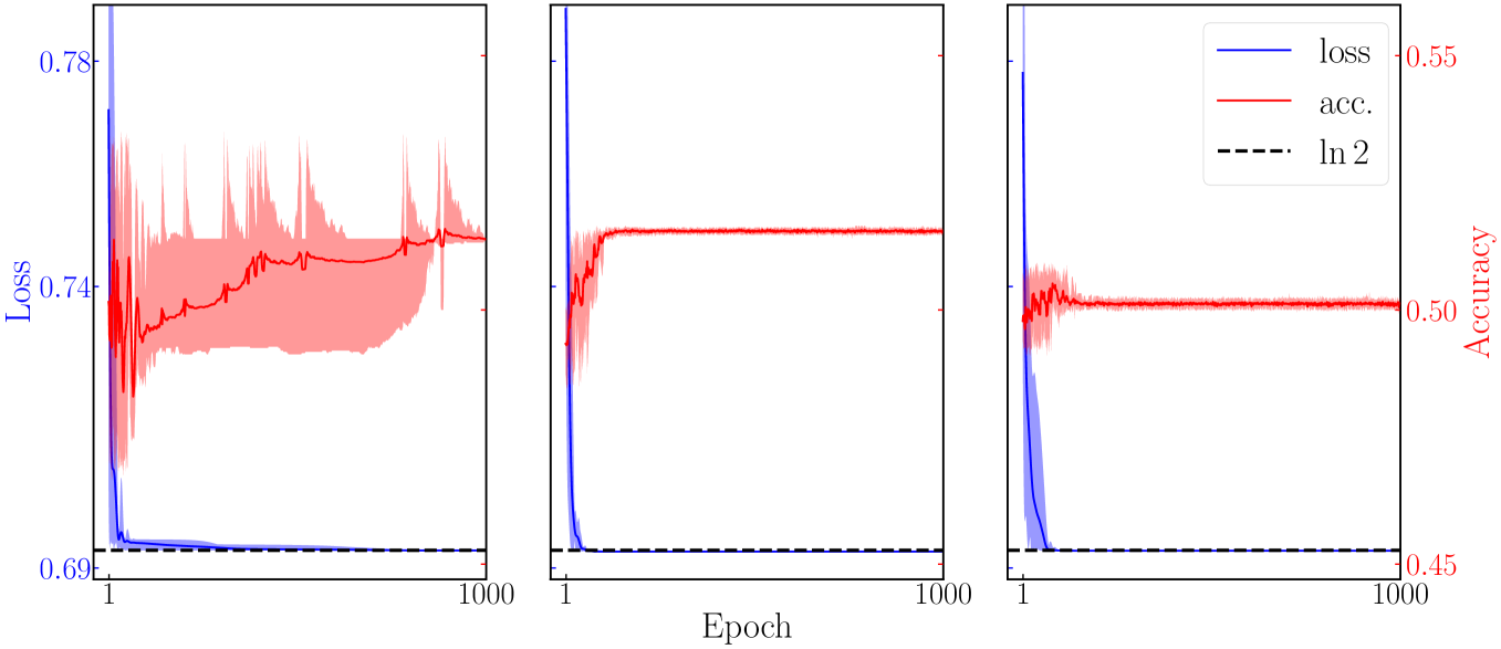
Figure C.1: Performance of the quantum classifier trained by a 1-layer circuit. From left to right, the figures show the training loss and accuracy for the datasets in Fig. 1(a), Fig. 2(a), and Fig. 3(a), respectively. The solid blue and red line, respectively, represent the mean of the training loss and accuracy over 10 runs, and the shaded areas represent their respective ranges across the 10 runs.

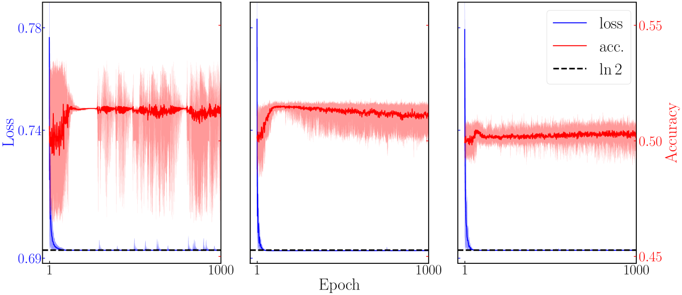
Figure C.2: Performance of the quantum classifier trained by a 10-layer circuit. From left to right, the figures show the training loss and accuracy for the datasets in Fig. 1(a), Fig. 2(a), and Fig. 3(a), respectively. The solid blue and red line, respectively, represent the mean of the training loss and accuracy over 10 runs, and the shaded areas represent their respective ranges across the 10 runs.

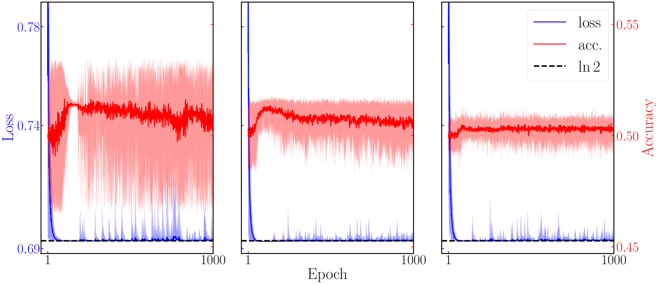
Figure C.3: Performance of the quantum classifier trained by a 30-layer circuit. From left to right, the figures show the training loss and accuracy for the datasets in Fig. 1(a), Fig. 2(a), and Fig. 3(a), respectively. The solid blue and red line, respectively, represent the mean of the training loss and accuracy over 10 runs, and the shaded areas represent their respective ranges across the 10 runs.

Appendix D QCNN circuit diagram

The 10-qubit QCNN circuit is shown in Fig. D.1. After amplitude encoding, the PQC consists of four convolutional layers (Conv) and pooling layers (Pool). In the pooling layers, one of the paired qubits is measured, and conditioned on the measurement result, a rotation is applied to the remaining qubit. The two-qubit gates are $XX(\theta)=e^{-i\frac{\theta}{2}(X\otimes X)}$, $YY(\theta)=e^{-i\frac{\theta}{2}(Y\otimes Y)}$, and $ZZ(\theta)=e^{-i\frac{\theta}{2}(Z\otimes Z)}$. The single-qubit gates are $R_{x}(\theta)=e^{-i\frac{\theta}{2}X}$, $R_{z}(\theta)=e^{-i\frac{\theta}{2}Z}$, where $X$, $Y$, and $Z$ are Pauli operators. The parameters of the variational gates are independent.

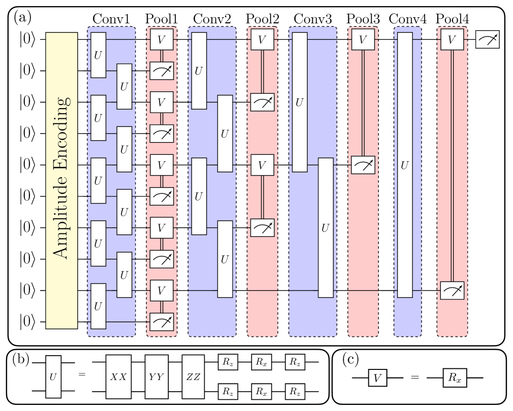
Figure D.1: (a) The architecture of QCNN. (b) The circuit for gate $U$. (c) The circuit for gate $V$.

References

- Biamonte et al. (2017) Jacob Biamonte, Peter Wittek, Nicola Pancotti, Patrick Rebentrost, Nathan Wiebe, and Seth Lloyd, “Quantum machine learning,” Nature 549, 195–202 (2017).
- Xiao et al. (2023) Tailong Xiao, Xinliang Zhai, Xiaoyan Wu, Jianping Fan, and Guihua Zeng, “Practical advantage of quantum machine learning in ghost imaging,” Commun. Phys. 6, 171 (2023).
- Azam and Kaiser (2024) Pierre Azam and Robin Kaiser, “Optically accelerated extreme learning machine using hot atomic vapors,” Phys. Rev. Appl. 22, 034041 (2024).
- Zheng et al. (2023) Pei-Lin Zheng, Jia-Bao Wang, and Yi Zhang, “Efficient and quantum-adaptive machine learning with fermion neural networks,” Phys. Rev. Appl. 20, 044002 (2023).
- LeCun et al. (1998) Yann LeCun, Léon Bottou, Yoshua Bengio, and Patrick Haffner, “Gradient-based learning applied to document recognition,” Proc. IEEE 86, 2278–2324 (1998).
- Krizhevsky et al. (2012) Alex Krizhevsky, Ilya Sutskever, and Geoffrey E Hinton, “ImageNet classification with deep convolutional neural networks,” in Proceedings of The 26th Conference on Neural Information Processing Systems (Curran Associates, Inc., Red Hook, NY, USA, 2012).
- Chen et al. (2024) Huanran Chen, Yinpeng Dong, Zhengyi Wang, Xiao Yang, Chengqi Duan, Hang Su, and Jun Zhu, “Robust classification via a single diffusion model,” in Proceedings of The 41st International Conference on Machine Learning (PMLR, New York, NY, USA, 2024).
- Schultheis et al. (2024) Erik Schultheis, Wojciech Kotlowski, Marek Wydmuch, Rohit Babbar, Strom Borman, and Krzysztof Dembczynski, “Consistent algorithms for multi-label classification with macro-at- metrics,” in Proceedings of The 12ed International Conference on Learning Representations (OpenReview.net, 2024).
- Raman and Tewari (2024) Vinod Raman and Ambuj Tewari, “Online classification with predictions,” in Proceedings of The 38th Conference on Neural Information Processing Systems (Curran Associates, Inc., Red Hook, NY, USA, 2024).
- Wang and Zhang (2024) Ming-Ming Wang and Xiao-Ying Zhang, “Quantum Bayes classifiers and their application in image classification,” Phys. Rev. A 110, 012433 (2024).
- Schuld et al. (2020) Maria Schuld, Alex Bocharov, Krysta M. Svore, and Nathan Wiebe, “Circuit-centric quantum classifiers,” Phys. Rev. A 101, 032308 (2020).
- Pérez-Salinas et al. (2020) Adrián Pérez-Salinas, Alba Cervera-Lierta, Elies Gil-Fuster, and José I Latorre, “Data re-uploading for a universal quantum classifier,” Quantum 4, 226 (2020).
- Henderson et al. (2020) Maxwell Henderson, Samriddhi Shakya, Shashindra Pradhan, and Tristan Cook, “Quanvolutional neural networks: powering image recognition with quantum circuits,” Quantum Mach. Intell. 2, 2 (2020).
- Hubregtsen et al. (2022) Thomas Hubregtsen, David Wierichs, Elies Gil-Fuster, Peter-Jan H. S. Derks, Paul K. Faehrmann, and Johannes Jakob Meyer, “Training quantum embedding kernels on near-term quantum computers,” Phys. Rev. A 106, 042431 (2022).
- Huang et al. (2021a) Hsin-Yuan Huang, Michael Broughton, Masoud Mohseni, Ryan Babbush, Sergio Boixo, Hartmut Neven, and Jarrod R McClean, “Power of data in quantum machine learning,” Nat. Commun. 12, 2631 (2021a).
- Xu et al. (2024) Li Xu, Xiao-yu Zhang, Ming Li, and Shu-qian Shen, “Quantum classifiers with a trainable kernel,” Phys. Rev. Appl. 21, 054056 (2024).
- Mitsuda et al. (2024) Naoki Mitsuda, Tatsuhiro Ichimura, Kouhei Nakaji, Yohichi Suzuki, Tomoki Tanaka, Rudy Raymond, Hiroyuki Tezuka, Tamiya Onodera, and Naoki Yamamoto, “Approximate complex amplitude encoding algorithm and its application to data classification problems,” Phys. Rev. A 109, 052423 (2024).
- Wang et al. (2024a) Yabo Wang, Xin Wang, Bo Qi, and Daoyi Dong, “Supervised-learning guarantee for quantum AdaBoost,” Phys. Rev. Appl. 22, 054001 (2024a).
- Liu et al. (2021) Yunchao Liu, Srinivasan Arunachalam, and Kristan Temme, “A rigorous and robust quantum speed-up in supervised machine learning,” Nat. Phys. 17, 1013–1017 (2021).
- Jerbi et al. (2023) Sofiene Jerbi, Lukas J. Fiderer, Hendrik Poulsen Nautrup, Jonas M. Kübler, Hans J. Briegel, and Vedran Dunjko, “Quantum machine learning beyond kernel methods,” Nat. Commun. 14, 517 (2023).
- Cong et al. (2019) Iris Cong, Soonwon Choi, and Mikhail D. Lukin, “Quantum convolutional neural networks,” Nat. Phys. 15, 1273–1278 (2019).
- Huang et al. (2021b) Hsin-Yuan Huang, Richard Kueng, and John Preskill, “Information-theoretic bounds on quantum advantage in machine learning,” Phys. Rev. Lett. 126, 190505 (2021b).
- Huang et al. (2022) Hsin-Yuan Huang et al., “Quantum advantage in learning from experiments,” Science 376, 1182–1186 (2022).
- Schuld and Killoran (2022) Maria Schuld and Nathan Killoran, “Is quantum advantage the right goal for quantum machine learning?” PRX Quantum 3, 030101 (2022).
- Cerezo et al. (2022) M. Cerezo, Guillaume Verdon, Hsin-Yuan Huang, Lukasz Cincio, and Patrick J. Coles, “Challenges and opportunities in quantum machine learning,” Nat. Comput. Sci. 2, 567–576 (2022).
- Lau et al. (2022) Jonathan Wei Zhong Lau, Kian Hwee Lim, Harshank Shrotriya, and Leong Chuan Kwek, “NISQ computing: where are we and where do we go?” AAPPS Bulletin 32, 27 (2022).
- (27) Maria Schuld, “Supervised quantum machine learning models are kernel methods,” ArXiv 2101.11020 .
- Caro et al. (2022) Matthias C Caro, Hsin-Yuan Huang, Marco Cerezo, Kunal Sharma, Andrew Sornborger, Lukasz Cincio, and Patrick J Coles, “Generalization in quantum machine learning from few training data,” Nat. Commun. 13, 4919 (2022).
- Benedetti et al. (2019) Marcello Benedetti, Erika Lloyd, Stefan Sack, and Mattia Fiorentini, “Parameterized quantum circuits as machine learning models,” Quantum Sci. Technol. 4, 043001 (2019).
- McClean et al. (2018) Jarrod R. McClean, Sergio Boixo, Vadim N. Smelyanskiy, Ryan Babbush, and Hartmut Neven, “Barren plateaus in quantum neural network training landscapes,” Nat. Commun. 9, 4812 (2018).
- Marrero et al. (2021) Carlos Ortiz Marrero, Mária Kieferová, and Nathan Wiebe, “Entanglement-induced barren plateaus,” PRX Quantum 2, 040316 (2021).
- Thanasilp et al. (2023) Supanut Thanasilp, Samson Wang, Nhat Anh Nghiem, Patrick Coles, and Marco Cerezo, “Subtleties in the trainability of quantum machine learning models,” Quantum Mach. Intell. 5, 21 (2023).
- Ragone et al. (2024) Michael Ragone, Bojko N Bakalov, Frédéric Sauvage, Alexander F Kemper, Carlos Ortiz Marrero, Martín Larocca, and M Cerezo, “A Lie algebraic theory of barren plateaus for deep parameterized quantum circuits,” Nat. Commun. 15, 7172 (2024).
- You and Wu (2021) Xuchen You and Xiaodi Wu, “Exponentially many local minima in quantum neural networks,” in Proceedings of The 38th International Conference on Machine Learning (PMLR, New York, NY, USA, 2021).
- Anschuetz and Kiani (2022) Eric R. Anschuetz and Bobak T. Kiani, “Quantum variational algorithms are swamped with traps,” Nat. Commun. 13, 7760 (2022).
- Zhang et al. (2022) Kaining Zhang, Liu Liu, Min-Hsiu Hsieh, and Dacheng Tao, “Escaping from the barren plateau via gaussian initializations in deep variational quantum circuits,” in Proceedings of The 35th Conference on Neural Information Processing Systems (Curran Associates, Inc., Red Hook, NY, USA, 2022).
- Wang et al. (2024b) Yabo Wang, Bo Qi, Chris Ferrie, and Daoyi Dong, “Trainability enhancement of parameterized quantum circuits via reduced-domain parameter initialization,” Phys. Rev. Appl. 22, 054005 (2024b).
- Meyer et al. (2023) Johannes Jakob Meyer, Marian Mularski, Elies Gil-Fuster, Antonio Anna Mele, Francesco Arzani, Alissa Wilms, and Jens Eisert, “Exploiting symmetry in variational quantum machine learning,” PRX Quantum 4, 010328 (2023).
- Huggins et al. (2019) William Huggins, Piyush Patil, Bradley Mitchell, K. Birgitta Whaley, and E. Miles Stoudenmire, “Towards quantum machine learning with tensor networks,” Quantum Sci. Technol. 4, 024001 (2019).
- Cerezo et al. (2021) M. Cerezo, Akira Sone, Tyler Volkoff, Lukasz Cincio, and Patrick J. Coles, “Cost function dependent barren plateaus in shallow parametrized quantum circuits,” Nat. Commun. 12, 1791 (2021).
- Larocca et al. (2023) Martin Larocca, Nathan Ju, Diego García-Martín, Patrick J. Coles, and Marco Cerezo, “Theory of overparametrization in quantum neural networks,” Nat. Comput. Sci. 3, 542–551 (2023).
- Caro et al. (2021) Matthias C. Caro, Elies Gil-Fuster, Johannes Jakob Meyer, Jens Eisert, and Ryan Sweke, “Encoding-dependent generalization bounds for parametrized quantum circuits,” Quantum 5, 582 (2021).
- Wiebe (2020) Nathan Wiebe, “Key questions for the quantum machine learner to ask themselves,” New J. Phys. 22, 091001 (2020).
- (44) Seth Lloyd, Maria Schuld, Aroosa Ijaz, Josh Izaac, and Nathan Killoran, “Quantum embeddings for machine learning,” ArXiv 2001.03622 .
- Weigold et al. (2021) Manuela Weigold, Johanna Barzen, Frank Leymann, and Marie Salm, “Expanding data encoding patterns for quantum algorithms,” in Proceddings of The 18th International Conference on Software Architecture Companion (IEEE Computer Society, Los Alamitos, CA, USA, 2021).
- Rath and Date (2024) Minati Rath and Hema Date, “Quantum data encoding: a comparative analysis of classical-to-quantum mapping techniques and their impact on machine learning accuracy,” EPJ Quantum Technol. 11, 72 (2024).
- Schuld and Petruccione (2018) Maria Schuld and Francesco Petruccione, Supervised Learning with Quantum Computers (Springer, Cham, Switzerland, 2018).
- LaRose and Coyle (2020) Ryan LaRose and Brian Coyle, “Robust data encodings for quantum classifiers,” Phys. Rev. A 102, 032420 (2020).
- Grant et al. (2018) Edward Grant, Marcello Benedetti, Shuxiang Cao, Andrew Hallam, Joshua Lockhart, Vid Stojevic, Andrew G Green, and Simone Severini, “Hierarchical quantum classifiers,” npj Quantum Inf. 4, 65 (2018).
- Hur et al. (2022) Tak Hur, Leeseok Kim, and Daniel K Park, “Quantum convolutional neural network for classical data classification,” Quantum Mach. Intell. 4, 3 (2022).
- Li et al. (2024) Qingyu Li, Yuhan Huang, Xiaokai Hou, Ying Li, Xiaoting Wang, and Abolfazl Bayat, “Ensemble-learning error mitigation for variational quantum shallow-circuit classifiers,” Phys. Rev. Res. 6, 013027 (2024).
- (52) Yann LeCun, “The MNIST database of handwritten digits,” http://yann.lecun.com/exdb/mnist/.
- Schuld et al. (2021) Maria Schuld, Ryan Sweke, and Johannes Jakob Meyer, “Effect of data encoding on the expressive power of variational quantum-machine-learning models,” Phys. Rev. A 103, 032430 (2021).
- Li et al. (2022) Guangxi Li, Ruilin Ye, Xuanqiang Zhao, and Xin Wang, “Concentration of data encoding in parameterized quantum circuits,” in Proceedings of The 35th Conference on Neural Information Processing Systems (Curran Associates, Inc., Red Hook, NY, USA, 2022).
- Schuld and Killoran (2019) Maria Schuld and Nathan Killoran, “Quantum machine learning in feature Hilbert spaces,” Phys. Rev. Lett. 122, 040504 (2019).
- Wang et al. (2021) Xinbiao Wang, Yuxuan Du, Yong Luo, and Dacheng Tao, “Towards understanding the power of quantum kernels in the NISQ era,” Quantum 5, 531 (2021).
- Thanasilp et al. (2024) Supanut Thanasilp, Samson Wang, M Cerezo, and Zoë Holmes, “Exponential concentration in quantum kernel methods,” Nat. Commun. 15, 5200 (2024).
- Giovannetti et al. (2008) Vittorio Giovannetti, Seth Lloyd, and Lorenzo Maccone, “Quantum random access memory,” Phy. Rev. Lett. 100, 160501 (2008).
- Park et al. (2019) Daniel K Park, Francesco Petruccione, and June-Koo Kevin Rhee, “Circuit-based quantum random access memory for classical data,” Sci. Rep. 9, 3949 (2019).
- Jiang et al. (2019) N Jiang, Y-F Pu, W Chang, C Li, S Zhang, and L-M Duan, “Experimental realization of 105-qubit random access quantum memory,” npj Quantum Inf. 5, 28 (2019).
- Plesch and Brukner (2011) Martin Plesch and Časlav Brukner, “Quantum-state preparation with universal gate decompositions,” Phys. Rev. A 83, 032302 (2011).
- Long and Sun (2001) Gui-Lu Long and Yang Sun, “Efficient scheme for initializing a quantum register with an arbitrary superposed state,” Phys. Rev. A 64, 014303 (2001).
- Araujo et al. (2021) Israel F Araujo, Daniel K Park, Francesco Petruccione, and Adenilton J da Silva, “A divide-and-conquer algorithm for quantum state preparation,” Sci. Rep. 11, 1–12 (2021).
- Gonzalez-Conde et al. (2024) Javier Gonzalez-Conde, Thomas W Watts, Pablo Rodriguez-Grasa, and Mikel Sanz, “Efficient quantum amplitude encoding of polynomial functions,” Quantum 8, 1297 (2024).
- Nakaji et al. (2022) Kouhei Nakaji, Shumpei Uno, Yohichi Suzuki, Rudy Raymond, Tamiya Onodera, et al., “Approximate amplitude encoding in shallow parameterized quantum circuits and its application to financial market indicators,” Phys. Rev. Res 4, 023136 (2022).
- Daimon and Matsushita (2024) Shunsuke Daimon and Yu-ichiro Matsushita, “Quantum circuit generation for amplitude encoding using a Transformer decoder,” Phys. Rev. Appl. 22, L041001 (2024).
- Fei et al. (2021) Nanyi Fei, Yizhao Gao, Zhiwu Lu, and Tao Xiang, “Z-score normalization, hubness, and few-shot learning,” in Proceedings of The 2021 IEEE/CVF International Conference on Computer Vision (IEEE Computer Society, Los Alamitos, CA, USA, 2021).
- Helber et al. (2019) Patrick Helber, Benjamin Bischke, Andreas Dengel, and Damian Borth, “EuroSAT: A novel dataset and deep learning benchmark for land use and land cover classification,” IEEE J. Sel. Top. Appl. Earth Obs. Remote Sens. 12, 2217–2226 (2019).
- Yang et al. (2023) Jiancheng Yang, Rui Shi, Donglai Wei, Zequan Liu, Lin Zhao, Bilian Ke, Hanspeter Pfister, and Bingbing Ni, “MedMNIST v2-A large-scale lightweight benchmark for 2D and 3D biomedical image classification,” Sci. Data 10, 41 (2023).
- Krizhevsky (2009) Alex Krizhevsky, “Learning multiple layers of features from tiny images,” (2009).
- Pesah et al. (2021) Arthur Pesah, Marco Cerezo, Samson Wang, Tyler Volkoff, Andrew T Sornborger, and Patrick J Coles, “Absence of barren plateaus in quantum convolutional neural networks,” Phys. Rev. X 11, 041011 (2021).
- Boyd and Vandenberghe (2004) Stephen P Boyd and Lieven Vandenberghe, Convex Optimization (Cambridge University Press, Cambridge, UK, 2004).
- Mohri et al. (2018) Mehryar Mohri, Afshin Rostamizadeh, and Ameet Talwalkar, Foundations of Machine Learning, 2nd ed. (The MIT Press, Cambridge, MA, USA, 2018).