Monge-Ampère gravitating fluids.
Least action principles and particle systems

Abstract.

The Monge-Ampère gravitation theory (MAG) was introduced by Brenier [8] to obtain an approximate solution of the early Universe reconstruction problem. It is a modification of Newtonian gravitation which is based on quadratic optimal transport. Later, Brenier [9], then Ambrosio, Baradat and Brenier [2] discovered a double large deviation principle for Brownian particles whose rate function is precisely MAG’s action functional.

In the present article, following Brenier we first recap MAG’s theory. Then, we slightly extend it from particles to fluid. This allows us to revisit the Ambrosio-Baradat-Brenier particle system and propose another one which is easier to interpret and whose large deviation rate function is MAG’s action functional for fluids.

This model leads to a Gibbs conditioning principle that is an entropy minimization problem close to the Schrödinger problem. While the setting of the Schrödinger problem is a system of noninteracting particles, the particle system we work with is subject to some branching mechanism which regulates the thermal fluctuations and some quantum force which balances them.

This article is dedicated to my long-time friend Patrick Cattiaux, on the occasion of his (official) retirement. CL.

Introduction

The Monge-Ampère gravitation (MAG) theory was introduced by Brenier in [8] to obtain an approximate solution of the early Universe reconstruction (EUR) problem. It is a modification of Newtonian gravitation which is based on quadratic optimal transport. Its action functional is, for any path $\omega=(\omega_{s})_{s_{0}\leq s\leq s_{1}}$ in $(\mathbb{R}^{d})^{k}$,

$$A(\omega):=\int_{s_{0}}^{s_{1}}\scalebox{1.2}{$\frac{1}{2}$}\|\dot{\omega}_{s}-\mathsf{v}_{s}(\omega_{s})\|^{2}\kappa_{s}\,ds,$$

for some specific velocity vector field $\mathsf{v}_{s}(x)$, some positive number $\kappa_{s}$ whose inverse $\kappa^{-1}_{s}$ is a diffusion coefficient and where as usual $\dot{\omega}_{s}:=d\omega_{s}/ds$ stands for the velocity of $\omega$. Any element of $(\mathbb{R}^{d})^{k}$ should be interpreted as a cloud of $k$ particles living in the configuration space $\mathbb{R}^{d}.$ Let us call any element of $(\mathbb{R}^{d})^{k}$ a $k$-mapping. See (3.9) for the exact formulation of the action functional.

A short note about action functionals and their link with the equations of motion is proposed at Appendix B.

The coexistence of $k$ particles is essential to convey (semi-discrete) optimal transport into the model.

A double large deviation principle

In two subsequent articles by Brenier, Ambrosio and Baradat [9, 2], MAG’s action functional was interpreted as the rate function of some double large deviation principle involving Brownian trajectories. More precisely, it happens that

$$A=\Gamma\textrm{-}\lim_{\epsilon\rightarrow 0}A^{\epsilon},\quad\textrm{where}\quad A^{\epsilon}(\omega)=\int_{s_{0}}^{s_{1}}\scalebox{1.2}{$\frac{1}{2}$}\|\dot{\omega}_{s}-\mathsf{v}^{\epsilon}_{s}(\omega_{s})\|^{2}\kappa_{s}\,ds,$$

and $\mathsf{v}^{\epsilon}$ is the current velocity of a rescaled Brownian motion in $(\mathbb{R}^{d})^{k}$

$$\mathsf{X}^{\epsilon}_{s}=\mathsf{X}_{s_{0}}+\sqrt{\epsilon}\ \mathsf{B}_{s},\quad s_{0}\leq s\leq s_{1},$$

see (3.8). Since the time marginal flow $(r^{\epsilon}_{s})_{s_{0}\leq s\leq s_{1}}$ of $\mathsf{X}^{\epsilon}$ solves the heat equation, we have

$$\partial_{s}r^{\epsilon}-\epsilon\Delta r^{\epsilon}/2=\partial_{s}r^{\epsilon}+\nabla\!\cdot\!(r^{\epsilon}\mathsf{v}^{\epsilon})=0,$$ (0.1)

with $\mathsf{v}^{\epsilon}_{s}=-\epsilon\nabla\log\sqrt{r^{\epsilon}_{s}}.$ In [2], the stochastic differential equation in $(\mathbb{R}^{d})^{k}$,

$$d\mathsf{Z}^{\epsilon,\eta}_{s}=\mathsf{v}^{\epsilon}_{s}(\mathsf{Z}^{\epsilon,\eta}_{s})\,ds+\sqrt{\eta\kappa_{s}^{-1}}\,d\mathsf{W}_{s},\quad 0<s_{0}\leq s\leq s_{1},$$ (0.2)

is introduced, where $\mathsf{W}$ is another $(\mathbb{R}^{d})^{k}$-valued Brownian motion, see (3.7). It is known that this collection of random evolutions obeys the Freidlin-Wentzell large deviation principle when the parameter $\eta$ tends to zero, $\epsilon$ being fixed,

$$\mathrm{Proba}(\mathsf{Z}^{\epsilon,\eta}\in\,\begin{picture}(-1.0,1.0)(-1.0,-3.0)\circle*{3.0}\end{picture}\ )\underset{\eta\to 0}{\asymp}\exp\left(-\eta^{-1}\ \inf_{\mathsf{z}\in\bullet}A^{\epsilon}(\mathsf{z})\right)$$

with rate function $A^{\epsilon}$, [17, 14]. Therefore, taking into account the already mentioned limit: $\Gamma\textrm{-}\lim_{\epsilon\rightarrow 0}A^{\epsilon}=A,$ we see that letting $\eta\to 0$, then $\epsilon\to 0,$ the family of Brownian diffusion processes $\mathsf{Z}^{\epsilon,\eta}$ obeys the double large deviation principle

$$\mathrm{Proba}(\mathsf{Z}^{\epsilon,\eta}\in\,\begin{picture}(-1.0,1.0)(-1.0,-3.0)\circle*{3.0}\end{picture}\ )\underset{\eta\to 0,\epsilon\to 0}{\asymp}\exp\left(-(\epsilon\eta)^{-1}\ \inf_{\mathsf{z}\in\bullet}A(\mathsf{z})\right)$$

with MAG’s action functional $A$ as its rate function. This also implies the Gibbs conditioning principle

$$\mathrm{Proba}(\mathsf{Z}^{\epsilon,\eta}\in\,\begin{picture}(-1.0,1.0)(-1.0,-3.0)\circle*{3.0}\end{picture}\ \mid\mathsf{Z}^{\epsilon,\eta}_{s_{0}}=\mathsf{z}_{0},\mathsf{Z}^{\epsilon,\eta}_{s_{1}}=\mathsf{z}_{1})\underset{\eta\to 0,\epsilon\to 0}{\asymp}\exp\left(-(\epsilon\eta)^{-1}\ \inf_{\mathsf{z}\in\bullet,\mathsf{z}(s_{0})=\mathsf{z}_{0},\mathsf{z}(s_{1})=\mathsf{z}_{1}}A(\mathsf{z})\right),$$

which in turns implies that, conditionally on $\mathsf{z}(s_{0})=\mathsf{z}_{0}$ and $\mathsf{z}(s_{1})=\mathsf{z}_{1},$ the most likely path of $\mathsf{Z}^{\epsilon,\eta}$ as $\eta\to 0$, then $\epsilon\to 0,$ solves MAG’s least action principle

$$\inf_{\mathsf{z}:\mathsf{z}(s_{0})=\mathsf{z}_{0},\mathsf{z}(s_{1})=\mathsf{z}_{1}}A(\mathsf{z}).$$

The stochastic evolution of $\mathsf{Z}^{\epsilon,\eta}$ is interpreted in [2] as a cloud of $k$ Brownian particles surfing the heat wave.

Aim of the article

The main goal of the present article is to revisit this interpretation. Indeed, the above model does not provide a clear physical picture. In particular, the forward velocity vector field $\mathsf{v}^{\epsilon}$ of $\mathsf{Z}^{\epsilon,\eta}$ happens to be the current velocity vector field of the other diffusion process: $\mathsf{X}^{\epsilon}.$ This enigmatic substitution is uneasy to interpret.

Another particle system

In the present paper, we drop the particle system $\mathsf{Z}^{\epsilon,\eta}$. But we keep [2]’s key idea of working with $\mathsf{X}^{\epsilon}$, because it establishes a crucial link with optimal transport: a central feature of MAG. We are going to investigate the large deviations of the empirical process of a family of branching Brownian particles, as their number tends to infinity. In absence of an extra force field, each branch is a copy of $\mathsf{X}^{\epsilon}.$ But to arrive at MAG, it is necessary that the whole system is immersed in some additional quantum force field.

From clouds to fluids

Passing to the limit as the number of particles tends to infinity, one does not work anymore with $k$-mappings, but with fluids, i.e. probability measures on $\mathbb{R}^{d}.$ In fact, we shall look at probability measures on $(\mathbb{R}^{d})^{k},$ i.e. fluids of $k$-mappings. We call these probability measures: $k$-fluids. Keeping $k$-mappings is essential to trace the effect of optimal transport. However, the relevant system to be observed is not the $k$-fluid, which contains the full details of the history of the $k$ particles that are necessary to play with optimal transport, but its one-particle marginal measure on $\mathbb{R}^{d}.$

We do not perform the limit $\epsilon\to 0.$ Neither do we look at the limit $k\to\infty,$ nor at the one-particle marginal projection of the $k$-fluid, leaving these steps to a forthcoming investigation. We only look at the fluid analog of the above action functional $A^{\epsilon},$ which is

$$(p_{s})_{s_{0}\leq s\leq s_{1}}\mapsto\int_{s_{0}}^{s_{1}}\scalebox{1.2}{$\frac{1}{2}$}\|\dot{\mathsf{p}}_{s}-\dot{\mathsf{r}}^{\epsilon}_{s}\|^{2}_{p_{s}}\,\kappa_{s}\,ds,$$ (0.3)

where $(p_{s})_{s_{0}\leq s\leq s_{1}}$ is a $k$-fluid-valued path, $\dot{\mathsf{p}}$ is its velocity in the Otto-Wasserstein (OW) manifold, $\|\,\begin{picture}(-1.0,1.0)(-1.0,-3.0)\circle*{3.0}\end{picture}\ \|_{p}$ is the norm of the tangent vector space at $p$ and

$$\dot{\mathsf{r}}^{\epsilon}_{s}=\mathsf{v}^{\epsilon}_{s}=-\epsilon\nabla\log\sqrt{r^{\epsilon}_{s}}$$

is the current velocity of the heat flow $(r^{\epsilon}_{s})_{s_{0}\leq s\leq s_{1}}$ – recall (0.1) – in the OW-manifold. We call the corresponding model: $\epsilon$-MAG for $k$-fluid.

Branching particles

Let us first briefly describe the branching mechanism; the quantum force will come later. We look at an empirical process $(\overline{X}^{N}_{s})_{s_{0}\leq s\leq s_{1}}$ such that for any $s,$ $\overline{X}^{N}_{s}$ is the empirical measure of $\lfloor\kappa_{s}N\rfloor$ particles in $(\mathbb{R}^{d})^{k}$ ($\lfloor a\rfloor$ denotes the integer part of the real number $a$). The factor $\kappa_{s}$ is analogous to $\kappa_{s}$ in formula (0.2). The trajectory of each particle is a copy of $\mathsf{X}^{\epsilon},$ but these copies are not independent. As $s\mapsto\kappa_{s}$ is an increasing function, during any small time interval $[s,s+h],$ a fraction $\kappa^{\prime}_{s}\,h+o_{h\to 0}(h)$ of the particles branch: each of them gives birth to a new particle starting at the same place as its genitor and evolving in the future according to the kinematics of $\mathsf{X}^{\epsilon}$ and independently of the other particles. Although the number of particles increases with time, $\overline{X}^{N}$ is normalized so that its total mass remains constant: $\overline{X}^{N}_{s}(\mathbb{R}^{dk})=1$ for all $s.$ As a consequence, the random fluctuation of $s\mapsto\overline{X}^{N}_{s}$ decreases with time. This branching mechanism acts as a cooling.

The large deviation rate function of $(\overline{X}^{N})_{N\geq 1}$ as $N$ tends to infinity leads us to the action functional

$$(p_{s})_{s_{0}\leq s\leq s_{1}}\mapsto\int_{s_{0}}^{s_{1}}\scalebox{1.2}{$\frac{1}{2}$}\|\dot{\mathsf{p}}_{s}-\dot{\mathsf{r}}^{\epsilon}_{s}\|^{2}_{p_{s}}\kappa_{s}\,ds+\epsilon^{2}\int_{s_{0}}^{s_{1}}I(p_{s}|r^{\epsilon}_{s})\kappa_{s}\,ds,$$ (0.4)

where $\displaystyle{I(p|r):=\int_{\mathbb{R}^{dk}}\scalebox{1.2}{$\frac{1}{2}$}\Big{|}\nabla\log\sqrt{\frac{dp}{dr}}\Big{|}^{2}\,dp}$ is the Fisher information of $p$ with respect to $r.$

Schrödinger problem

Without any branching, that is if the function $\kappa$ is equal to $1,$ $\overline{X}^{N}$ is the usual empirical process of an iid sample of $\mathsf{X}^{\epsilon}$ and the action functional becomes

$$(p_{s})_{s_{0}\leq s\leq s_{1}}\mapsto\int_{s_{0}}^{s_{1}}\scalebox{1.2}{$\frac{1}{2}$}\|\dot{\mathsf{p}}_{s}-\dot{\mathsf{r}}^{\epsilon}_{s}\|^{2}_{p_{s}}\,ds+\epsilon^{2}\int_{s_{0}}^{s_{1}}I(p_{s}|r^{\epsilon}_{s})\,ds.$$ (0.5)

It corresponds to the dynamics of an entropic interpolation, i.e. the time marginal flow $(p_{s}=P_{s})_{s_{0}\leq s\leq s_{1}}$ of the solution $P$ of the Schrödinger problem

$$\inf_{P:P_{s_{0}}=p_{s_{0}},P_{s_{1}}=p_{s_{1}}}H(P|R^{\epsilon}),$$

where $R^{\epsilon}$ is the law of $\mathsf{X}^{\epsilon},$ $P$ is a path measure and

$$H(P|R^{\epsilon}):=\int\log(dP/dR^{\epsilon})\,dP$$

is the relative entropy of $P$ with respect to $R^{\epsilon}.$ The "branching modification" that is described above permits to pass from (0.5) to (0.4).

Quantum force

To arrive at MAG’s action functional (0.3), it suffices to subtract $\epsilon^{2}\int_{s_{0}}^{s_{1}}I(p|r^{\epsilon}_{s})\kappa_{s}\,ds$ from (0.5). It is convenient to express this operation by means of the corresponding Newton equation of motion in the OW-manifold. Also, things are clearer after doing some change of time, see the parameter setting 3.10, to arrive at

$$(q_{t})_{t_{0}\leq t\leq t_{1}}\mapsto \int_{t_{0}}^{t_{1}}\scalebox{1.2}{$\frac{1}{2}$}\|\dot{\mathsf{q}}_{t}-\dot{\mathsf{m}}^{\epsilon}_{t}\|^{2}_{q_{t}}\,dt$$ (0.6)

$$(q_{t})_{t_{0}\leq t\leq t_{1}}\mapsto \int_{t_{0}}^{t_{1}}\scalebox{1.2}{$\frac{1}{2}$}\|\dot{\mathsf{q}}_{t}-\dot{\mathsf{m}}^{\epsilon}_{t}\|^{2}_{q_{t}}\,dt+\epsilon^{2}\int_{t_{0}}^{t_{1}}\sigma_{t}I(q_{t}|m^{\epsilon}_{t})\,dt,$$ (0.7)

instead of (0.3) and (0.4). Here $\dot{\mathsf{m}}^{\epsilon}_{t}$ is the velocity of the time-changed heat flow $(m^{\epsilon}_{t})$ in the OW-manifold, see (5.7) and (5.8), and $t\mapsto\sigma_{t}$ is some positive function, see (9.2).
We show that the Newton equation corresponding to $\epsilon$-MAG’s action functional (0.6) is

$$\ddot{\mathsf{q}}_{t}=\ddot{\mathsf{m}}^{\epsilon}_{t}.$$ (0.8)

This is the equation of motion of $\epsilon$-MAG for a $k$-fluid.
In terms of an equation of motion, subtracting the Fisher information term from the action functional (0.7) arising from the large deviations of $\overline{X}^{N},$ amounts to apply the force field

$$-\epsilon^{2}\sigma_{t}\operatorname{grad}^{\mathrm{OW}}_{q_{t}}I(\,\begin{picture}(-1.0,1.0)(-1.0,-3.0)\circle*{3.0}\end{picture}\ |m^{\epsilon}_{t}).$$

It is a quantum force field, because we show (informally) that any solution $\Psi$ (wave function) of the nonlinear Schrödinger equation

$$\big{(}-i\hbar\partial_{t}-\hbar^{2}\Delta/2-\hbar^{2}\mathcal{Q}(m^{\epsilon}_{t}|\mathrm{Leb})\big{)}\Psi+(\sigma_{t}{\epsilon^{2}}-\hbar^{2})\mathcal{Q}(|\Psi|^{2}|m^{\epsilon}_{t}))=0,$$ (0.9)

is such that $q=|\Psi|^{2}$ solves the Newton equation

$$\ddot{\mathsf{q}}_{t}=-\epsilon^{2}\sigma_{t}\operatorname{grad}^{\mathrm{OW}}_{q_{t}}I(\,\begin{picture}(-1.0,1.0)(-1.0,-3.0)\circle*{3.0}\end{picture}\ |m^{\epsilon}_{t}).$$ (0.10)

Here $\hbar$ is Planck’s constant and $\mathcal{Q}(\,\begin{picture}(-1.0,1.0)(-1.0,-3.0)\circle*{3.0}\end{picture}\ |\mathrm{Leb})$ and $\mathcal{Q}(\,\begin{picture}(-1.0,1.0)(-1.0,-3.0)\circle*{3.0}\end{picture}\ |m^{\epsilon}_{t})$ are quantum potentials defined at (9.11). This derivation is inspired from von Renesse’s article [34].

Picking up the pieces

We conclude that the equation of motion, as $N$ tends to infinity, of the branching Brownian particle system $\overline{X}^{N},$ immersed in the above quantum force field, is $\epsilon$-MAG’s equation of motion (0.8).

Stepping back to model (0.2), the parameter $N$ replaces $\eta,$ the branching mechanism replaces the parameter $\kappa$ in the factor $\sqrt{\eta\kappa_{s}^{-1}}\,d\mathsf{W}_{s},$ and the quantum force field supersedes the enigmatic substitution of the forward velocity of $\mathsf{Z}^{\epsilon,\eta}$ by the the current velocity of $\mathsf{X}^{\epsilon}$.

Outline of the article

Section 1 begins with a short description of the physical basis of the Monge-Ampère gravitation theory. We also sketch the early Universe reconstruction problem as the main motivation for this modified theory of gravitation. Section 2 is dedicated to the exposition of the mathematics of MAG, as introduced by Brenier in [8], and Section 3 gives the details about the model (0.2) which is the main object of the article [2] by Ambrosio, Baradat and Brenier. At Section 4, we introduce the analogs for fluids of the action functionals $A$ and $A^{\epsilon}$, such as (0.3). This is the place where some basic material about the Otto-Wasserstein geometry is gathered; some more is presented at the beginning of Section 6. The action functional (0.3)/(0.6) we mainly work with is introduced at Section 5.

Newton’s equation of motion (0.8) is proved at Section 6. A detailed description of the acceleration $\ddot{\mathsf{q}}$ is also obtained at Theorem 6.2. It reveals divergences of the force field at some specific places which are responsible for the concentration of matter.

The last three sections are dedicated to the construction of the particle system that was presented during this introductory section. At Section 7, we recall already known facts about the dynamics of the solutions of the Schrödinger problem. This leads us to the action functional (0.5). Then, we introduce the factor $\kappa_{s}$, at Section 8 to arrive at the action functional (0.4). This is the place where we prove that the branching mechanism that was previously described transforms (0.5) into (0.4). Finally, at Section 9, the quantum force (0.10) is shown to be associated with the nonlinear Schrödinger equation (0.9).

Sections 1, 2, 3 and 7 are expository: most of their content is already known. The rest of the article consists of new material.

This program of investigation is far from being complete: a short list of remaining things to be done is proposed at Appendix A. We also provide at Appendix B a basic reminder about the minimization of action functionals, and at Appendix C some simple analogies are presented to illustrate the concentration of matter that results from MAG’s dynamics.

1. MAG. Motivation and definition

Newtonian gravitation

The equation of motion of a test particle in gravitational interaction with a fluid is

$$\ddot{x}_{t}=-\nabla\varphi_{t}(x_{t}),\quad t\geq 0,$$ (1.1)

where the scalar potential $\varphi$ solves the Poisson equation

$$\Delta\varphi_{t}=\mu_{t}.$$ (1.2)

Here, $x_{t}\in\mathbb{R}^{d}$ is the position of the test particle at time $t$, $\ddot{x}_{t}$ is its acceleration and $\mu_{t}(x)$ is the density of the fluid at time $t$ and location $x.$ While Newton’s equation (1.1) is physically correct (the mass of the test particle is irrelevant), for simplicity we do not write the gravitational constant in (1.2).

In computational cosmology, the configuration space $\mathbb{R}^{d}$ is replaced by the flat torus

$$\mathbb{T}^{d}_{L}=\mathbb{R}^{d}/[0,L]^{d}$$

with size $L>0$. Assuming that $\mu_{t}(\mathbb{T}^{d}_{L}):=\int_{\mathbb{T}^{d}_{L}}\mu_{t}(x)\,dx<\infty,$ without loss of generality one can normalize $\mu_{t}$ as a probability measure.
Periodic boundary conditions imply that for any regular $[0,L]^{d}$-periodic function $\varphi$

$$\int_{[0,L]^{d}}\Delta\varphi\,d\mathrm{Leb}=\int_{\mathbb{R}^{d}}\mathbf{1}_{[0,L]^{d}}\nabla\!\cdot\!(\nabla\varphi)\,d\mathrm{Leb}\\ =-\int_{\mathbb{R}^{d}}\nabla\mathbf{1}_{[0,L]^{d}}\!\cdot\!\nabla\varphi\,d\mathrm{Leb}=\int_{\partial[0,L]^{d}}\nabla\varphi\cdot\vec{n}\,d\sigma=0$$

where $\mathrm{Leb}$ stands for the Lebesgue measure, $\vec{n}$ is the outer unit normal vector on the boundary $\partial[0,L]^{d}$ of $[0,L]^{d}$ equipped with the surface measure $\sigma=\mathrm{Leb}_{|\partial[0,L]^{d}}.$ This is Stokes formula and its vanishing means that the mass of any distribution of matter evolving along the integral curves of the vector field $\nabla\varphi$ remains constant since $\mathbb{T}^{d}_{L}$ has no physical boundary.
Hence, for a Poisson equation in $\mathbb{T}^{d}_{L}$ to admit a solution it is necessary that its right hand term has a zero mass. Let us replace equation (1.2) by $\Delta\varphi_{t}=\mu_{t}-\lambda$ where $\lambda$ is some probability measure on $\mathbb{T}^{d}_{L}.$ The best natural choice for $\lambda$ is the uniform unit volume measure on the torus

$$\lambda_{L}=L^{-d}\ \mathrm{Leb}_{|\mathbb{T}^{d}_{L}}.$$

Indeed, doing this we see that, with the balanced Poisson equation

$$\Delta\varphi_{t}=\mu_{t}-\lambda_{L}\quad\textrm{on }\mathbb{T}^{d}_{L},$$ (1.3)

a uniform distribution of matter: $\mu_{t}=\lambda_{L},$ does not generate any gravitational force, as expected. Moreover, it successfully passes the “large box”-test

$$\lim_{L\to\infty}\eqref{eq-03}=\eqref{eq-02}.$$ (1.4)

Indeed, letting $L$ tend to infinity, one recovers the standard Poisson equation (1.2) in $\mathbb{R}^{d}$ because the background source term $\lambda_{L}$ vanishes as $L$ tends to infinity. For further physical justification of this model in cosmology, see [21, 5].

Monge-Ampère gravitation (MAG)

Brenier [8] introduced a modified theory of gravitation which, although not fundamental, is effective for solving the early Universe reconstruction (EUR) problem. The main feature of this modified theory consists in replacing the Poisson equation (1.3) by the Monge-Ampère equation

$$L^{-d}\det(\mathbb{I}+\operatorname{Hess}(L^{d}\varphi_{t}))=\mu_{t},\quad\textrm{on}\ \mathbb{T}^{d}_{L},$$ (1.5)

where $\mathbb{I}$ is the identity matrix. The couple of equations (1.1) and (1.5) is called Monge-Ampère gravitation, MAG for short. Note that (1.5) admits (1.3) as its linearization in the limit of weak gravitation, that is

$$\lim_{\|\operatorname{Hess}\varphi\|\to 0}\eqref{eq-04b}=\eqref{eq-03},$$

or more precisely $\Delta\varphi_{t}=\mu_{t}-\lambda_{L}+o_{\|\operatorname{Hess}\varphi_{t}\|\to 0}(\|\operatorname{Hess}\varphi_{t}\|),$ $L$ being fixed. Moreover, it is exactly (1.3) in dimension one. But in dimension $d\geq 2,$ it fails the “large box”-test:

$$\lim_{L\to\infty}\eqref{eq-04b}\neq\eqref{eq-02}.$$

For instance, in dimension $d=3,$

$$L^{-3}\det(\mathbb{I}+\operatorname{Hess}(L^{3}\varphi)) =L^{-3}\det(\mathbb{I}+L^{3}\mathrm{diag}(a,b,c))=L^{-3}(1+L^{3}a)(1+L^{3}b)(1+L^{3}b)$$

$$=L^{-3}+\Delta\varphi+L^{3}(ab+ac+bc)+L^{6}abc,$$ (1.6)

where $a,b$ and $c$ are the eigenvalues of $\operatorname{Hess}\varphi.$ We see that the dominating term as $L$ tends to infinity is not $\Delta\varphi$ as desired, but $L^{6}\det(\operatorname{Hess}\varphi).$ This remains true in any dimension where the dominating term is $L^{d^{2}-d}\det(\operatorname{Hess}\varphi)$.
Moreover, when $d\geq 2$, there is no mixed asymptotic regime $(L\to\infty,\|\operatorname{Hess}\varphi\|\to 0),$ where (1.3)&(1.5) is an approximation of Newtonian gravity which would be valid for any $\varphi.$ Let us show it. Denoting $H:=\|\operatorname{Hess}\varphi\|$, we see that

$$L^{-d}\det(\mathbb{I}+\operatorname{Hess}(L^{d}\varphi))=\Delta\varphi+L^{-d}+L^{-d}\sum_{2\leq n\leq d}O((L^{d}H)^{n}).$$

A regime where $\Delta\varphi$ would be the dominating term, must satisfy

$$H^{-1}\Big{(}L^{-d}+L^{-d}\sum_{2\leq n\leq d}O((L^{d}H)^{n})\Big{)}\longrightarrow 0,$$

because $\Delta\varphi=O(H)\rightarrow 0.$ Since this term is of order $(L^{d}H)^{-1}+\sum_{1\leq n\leq d-1}(L^{d}H)^{n},$ this would imply that $L^{d}H$ tends simultaneously to $\infty$ and $0$, a contradiction. $\square$

Nevertheless, despite this negative result, MAG reveals to be effective for approximately solving the early Universe reconstruction problem. This is illustrated by Figure 2 and will be partly explained during a short discussion at page 1.

Early Universe reconstruction (EUR)

This problem was addressed by Peebles in the seminal paper [30]. One specific feature with cosmology is that the distribution of matter/energy of the very early Universe was highly uniform as testified by the observation of the cosmic microwave background which exhibits a relative fluctuation from uniformity of order $10^{-4}$: typically $3K\pm 300\mu K$ (the unit $K$ is a Kelvin degree).

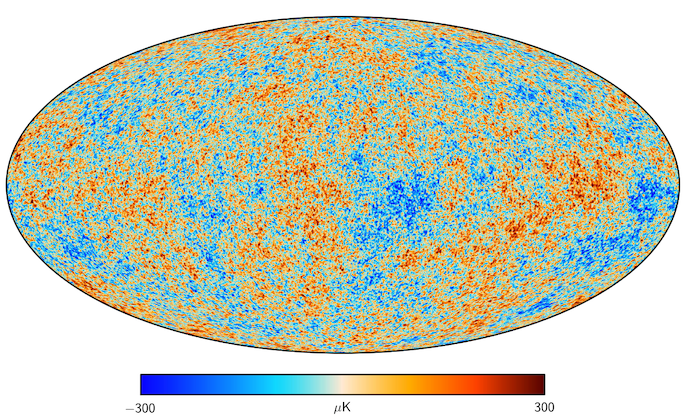
Figure 1. Cosmic microwave background

This very peculiar property of the initial condition is one reason for the Monge-Ampère strategy to be successful when solving EUR. However, the other reasons for its effectiveness are not fully understood at present time. We hope that this article will be a step towards a clearer picture.
One aim of EUR is to give estimates of the field of very early fluctuations from this uniformity

$$\mu^{\prime}_{0}(x):=\lim_{t\to 0^{+}}\frac{\mu_{t}(x)-L^{-d}}{t},$$

a crucial information to test the cosmic inflation theory and provide details about the initial quantum fluctuations.

An effective theory in computational cosmology

As an illustration of the good performance of MAG in cosmology, we provide at Figure 2 a couple of images representing typical structures of the actual Universe. Both are obtained by running numerical simulations starting from the same initial condition: a tiny perturbation of the uniform measure on $\mathbb{T}^{3}_{L}.$ The left-hand side image (A) is obtained using the balanced Poisson equation (1.3), while the right-hand side (B) results from using the Monge Ampère equation (1.5) instead of the physically more realistic law (1.3).

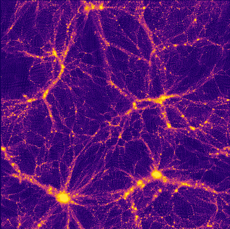
(a) Poisson

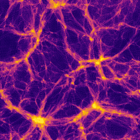
(b) Monge-Ampère

Figure 2. Typical structures of the actual Universe
Courtesy of Bruno Lévy

MAG works well with EUR

Let us discuss a little bit about MAG being a good approximation of the Newtonian gravity in the special setting of the EUR problem. The symmetric operator $\operatorname{Hess}\varphi$ admits an orthogonal basis of eigenvectors. Let $K:=\{x\in\mathbb{R}^{3};\operatorname{Hess}\varphi(x)=0\}$ denotes its kernel, and $K^{\perp}$ be $K$’s orthogonal subspace in $\mathbb{R}^{3}.$ Suppose that $\operatorname{Hess}\varphi$ admits at least one zero eigenvalue and at least one non-zero one. This means that both $K$ and $K^{\perp}$ are eigenspaces and that $(\mathrm{dim}(K),\mathrm{dim}(K^{\perp}))$ is either $(1,2)$ or $(2,1).$ Since $\operatorname{Hess}\varphi$ is the Jacobian matrix $\mathrm{Jac}(\nabla\varphi)$ of the opposite of the acceleration field $\ddot{x}=-\nabla\varphi,$ this implies that the acceleration is locally constant in direction $K$, so that any concentration of matter in direction $K^{\perp}$ is pushed by a force field in direction $K$, possibly fostering the formation of a structure of dimension $\mathrm{dim}(K).$

1. At places where $\operatorname{Hess}\varphi$ admits a single zero-eigenvalue, that is $\mathrm{dim}(K)=1,$ then 1D singular structures (filaments) might appear.

2. At places where $\operatorname{Hess}\varphi$ admits a double zero-eigenvalue, that is $\mathrm{dim}(K)=2,$ then 2D singular structures (sheets) might appear.

Going back to (1.6), it appears that (1.5) is exactly (1.3) if two eigenvalues of $\operatorname{Hess}\varphi$ vanish. In practice, for MAG being close to Newtonian gravitation, one eigenvalue should be very close to zero to kill the leading term $L^{6}abc$ and another one should be small enough to control the intermediate term $L^{3}(ab+ac+bc).$
As can be seen at Figure 2(a), it happens that N-body simulations based on the Newtonian gravitation reveal that, after some time, most of the matter is concentrated in singular structures: sheets and filaments (Figure 2 depicts 2D-slices of 3D-cubes). This is a clue in favor of the good fit between these two theories in this special case. However, estimating the accuracy of MAG for solving EUR still remains a mathematical open problem.

Remark that the above classification of singular structures in terms of $\operatorname{Hess}\varphi$ differs from the standard approach by Zeldovich [36] which is based on the Jacobian of a velocity field rather than an acceleration field. The way our classification complements Zeldovich’s one will be explored elsewhere.

Pro and cons

From a practical point of view, one advantage of MAG is that it provides us with faster computations than the standard Poisson-based algorithms, because of its connection with optimal transport (this will be made precise later). More about cosmological simulations using MAG and their comparison with standard N-body simulations can be found in the recent article [25] by Lévy, Brenier and the second author. From a theoretical point of view, another advantage is that its tight relation with optimal transport provides us with easy geometrical interpretations. Moreover, it is shown in the article [6] by Bonnefous, Brenier and one of us (RM) that MAG can describe a scalar field, often evoked in modified theories of gravity such as Galileons, opening a promising domain to further explore.
However, the main drawback of MAG is that it is not a fundamental theory of gravitation; it is only effective for solving EUR.

From now on we drop the size $L$ by setting $L=1$, and denote $\mathbb{T}^{d}=\mathbb{T}_{L=1}^{d}.$

Zeldovich approximation

In [8] Brenier transposed Peebles’ EUR problem in the framework of the semi-Newtonian gravitational model of the early Universe where the trajectory $t\mapsto x_{t}\in\mathbb{T}^{3}$ of each particle (typically a cluster of galaxies!) satisfies the Newton-like equation of motion

$$\frac{2t}{3}\ddot{x}_{t}+\dot{x}_{t}=-\nabla\varphi_{t}(x_{t}),\quad t\geq 0,$$ (1.7)

where the potential $\varphi$ solves

$$1+t\Delta\varphi_{t}=\mu_{t}$$ (1.8)

and $\mu_{t}$ is the matter density. This describes classical Newtonian interactions taking place in an Einstein-de Sitter space corresponding to a Big Bang scenario. The couple of equations (1.7)&(1.8) is called the semi-Newtonian system (SNS).
At time $t=0,$ we see that

$$\mu_{0}\equiv 1,\quad\dot{x}_{0}=-\nabla\varphi_{0}(x_{0}),\quad\Delta\varphi_{0}(x)=\lim_{t\to 0^{+}}\frac{\mu_{t}(x)-1}{t}=:\mu^{\prime}_{0}(x).$$

Remarks 1.9.

1. One is far from the classical $N$-body problem.

2. Equation (1.8) is simply (1.3) with $L=1$ and $t\varphi_{t}$ instead of $\varphi_{t}.$

3. The physical assumption: $\mu_{0}\equiv 1,$ is experimentally verified up to a very high precision level, see Figure 1.

Zeldovich approximation [36] is simply

$$\widetilde{x}_{t}=x_{0}-t\nabla\varphi_{0}(x_{0}),\qquad 0\leq t\leq t_{*}(x_{0}),$$

where $0<t_{*}(x_{0})\leq\infty$ is the first time where a collision with another particle occurs. In this scenario, the initial fluctuation of the field generates a path with constant velocity until its first collision.

Brenier proved in [8] that keeping (1.7), but replacing the balanced Poisson equation (1.8) by the Monge-Ampère equation

$$\det(\mathbb{I}+t\operatorname{Hess}\varphi_{t})=\mu_{t},$$ (1.10)

one obtains a least action principle admitting the Zeldovich approximations as its exact solutions. A similar reasoning will be exposed in a while to arrive at (2.19) for the MAG problem (1.1)&(1.13), see Definition 1.12 below. Note that (1.8) and (1.10) are exactly (1.3) and (1.5) with $L=1$ and different notations for the potential.

Optimal transport versus N-body simulation

Frisch, Matarrese, Sobolevskii and the second author of the present article have shown in [18], more than twenty years ago, that with the simplified dynamics of the Zeldovich approximation, EUR  is exactly the Monge quadratic optimal transport problem between the initial uniform distribution of matter $\mu_{0}\equiv 1$ and the distribution of matter of the present epoch $\mu_{T},$ provided that the Zeldovich map $x_{0}\mapsto\widetilde{x}_{T}(x_{0})$ is the gradient of a convex potential. See also [10] for more mathematical details. Numerical simulations in [18] also demonstrate that the solution of this quadratic optimal transport problem is close to the result of $N$-body simulations as performed following [21, 5] for instance. Figure 3 illustrates the comparison between a standard N-body simulation and a construction using optimal transport. More precisely, one compares the joint distributions of the couples of initial and final positions of the N-body simulation with the optimal transport plan between the initial and final marginal distributions of the N-body simulation. The yellow points of the left-hand side picture correspond to significant errors of matching. The dots near the diagonal on the right-hand side graphic are a scatter plot of reconstructed (using optimal transport) initial points vs. simulation initial points. The upper left inset is a histogram (by percentage) of distances between such points; 62% are assigned exactly (up to the grid precision). The lower right inset is a similar histogram for reconstruction on a finer grid where 34% are assigned exactly.

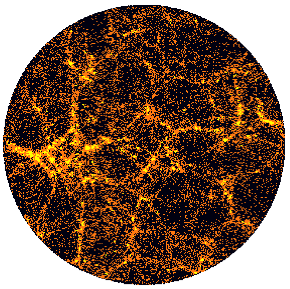
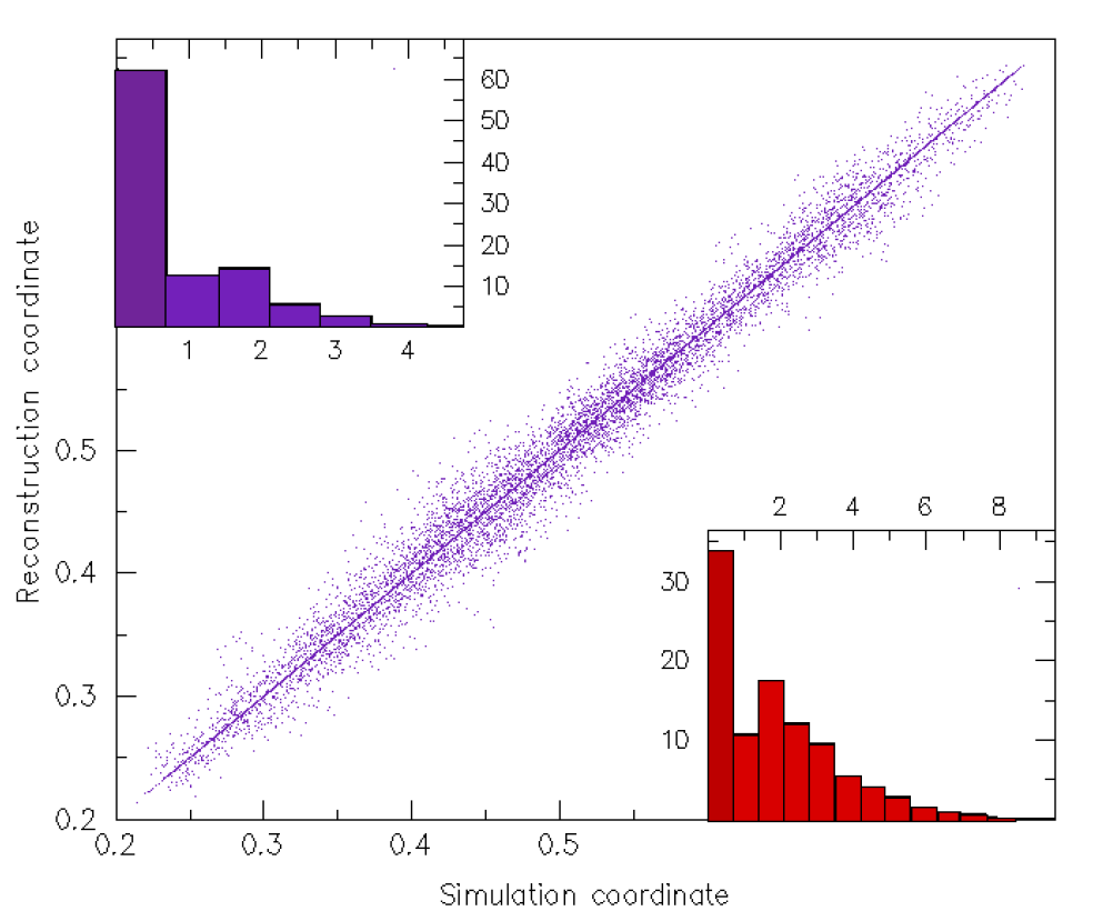
Figure 3. Optimal transport vs. N-body simulation, [18].

MAG’s definition

The first definition of MAG that appeared in the literature is the following

Definition 1.11 (MAG’s approximation of SNS, [8]).

On the torus $\mathbb{T}^{d}=\mathbb{R}^{d}/[0,1]^{d},$ the dynamics defined by the couple of equations (1.7)&(1.10) is the Monge-Ampère gravitation (MAG) system approximating the semi-Newtonian system (SNS) (1.7)&(1.8).

MAG’s approximation of SNS is effective in the regime of short time and weak gravity.

From now on, following Brenier and his co-authors [9, 1, 2] we drop the relativistic dynamics (1.7) and go back to the usual Newton equation (1.1). With this choice the underlying physics is less realistic, but the mathematics are clearer and easier to handle. This simplification seems to us to be a reasonable choice for a preliminary approach of a more complete theory to be developed later.

Definition 1.12 (MAG on $\mathbb{T}^{d}$, absolutely continuous fluid, [8]).

The dynamics defined on the torus $\mathbb{T}^{d}=\mathbb{R}^{d}/[0,1]^{d}$ by the couple of equations (1.1) and

$$\det(\mathbb{I}+\operatorname{Hess}\varphi_{t})=\mu_{t},\quad\textrm{on}\ \mathbb{T}^{d},$$ (1.13)

is called Monge-Ampère gravitation, MAG for short.

Furthermore, to simplify the mathematics and the presentation, we keep Brenier’s choice in [8, 2] to consider MAG  in the whole space $\mathbb{R}^{d}$ rather than in the torus $\mathbb{T}^{d},$ see Definition 2.6 below. However, a severe critic of this choice is expressed at Remark 2.9-(i).

2. MAG. Action functional

This section is aimed at giving a short presentation of the Monge-Ampère gravitation theory. It describes step by step the way for justifying Brenier’s Definition 2.26 of MAG’s action functional.

Optimal transport

At first sight, it seems to be useless to replace the linear equation (1.3) by a nonlinear one. But, be aware that solving the gravitational problem (1.1)&(1.3), or its standard counterpart (1.1)&(1.2), remains inaccessible in most situations. On the other hand, as will be seen in a moment, the connection of the Monge-Ampère equation (1.13) with quadratic optimal transport permits a rather simple geometric interpretation of MAG which leads to a fast numerical algorithm in [8].

Following Brenier [8], let us make precise the connection of (1.13) with quadratic optimal transport. Take a probability measure $\lambda$ on $\mathbb{R}^{d}$ and transport it by the measurable map ${\overrightarrow{T}}:\mathbb{R}^{d}\to\mathbb{R}^{d}$ to obtain its image

$$\mu:={\overrightarrow{T}}_{\#}\lambda,$$

defined by $\mu(dy)=\lambda\big{(}({\overrightarrow{T}})^{-1}(dy)\big{)}.$ We have in mind that $\mu$ plays the role of the actual distribution of matter. The measure $\lambda$ will be specified at (2.5) so that some analogue of (1.13) is satisfied, see (2.7) below.
If $\mu$ is absolutely continuous and ${\overrightarrow{T}}$ is injective and differentiable almost everywhere, then $\lambda$ is also absolutely continuous, the inverse map $({\overrightarrow{T}})^{-1}=:\overleftarrow{T}$ is differentiable $\mu$-a.e., $\overleftarrow{T}_{\#}\mu=\lambda$ and the Monge-Ampère equation

$$\mu(y)=\lambda(\overleftarrow{T}(y))\ |\det(\nabla\overleftarrow{T})(y)|,\quad y\in\mathbb{R}^{d},\ \textrm{a.e.}$$ (2.1)

is satisfied. Here and in the remainder of this article, any absolutely continuous measure and its density with respect to Lebesgue measure are denoted by the same letter.
The Monge optimal transport problem which is relevant for our purpose is

$$\inf_{\overleftarrow{T}:\overleftarrow{T}_{\#}\mu=\lambda}\int_{\mathbb{R}^{d}}|y-\overleftarrow{T}(y)|^{2}\,\mu(dy),$$ (2.2)

where, as for equation (2.1), the unknown is the map $\overleftarrow{T}:\mathbb{R}^{d}\to\mathbb{R}^{d}$, while the probability measures $\lambda$ and $\mu$ are prescribed. Brenier’s theorem [7] tells us that when $\int_{\mathbb{R}^{d}}|x|^{2}\,\lambda(dx)<\infty,$ $\int_{\mathbb{R}^{d}}|y|^{2}\,\mu(dy)<\infty$ and $\mu$ is absolutely continuous, (2.2) admits a unique solution $\overleftarrow{T}$. Moreover,

$$\overleftarrow{T}=\nabla\theta,\quad\textrm{a.e.,}$$ (2.3)

where $\theta:\mathbb{R}^{d}\to\mathbb{R}$ is a convex function. As Aleksandrov’s theorem states that any convex function on $\mathbb{R}^{d}$ is twice differentiable almost everywhere, the Jacobian matrix $\nabla\overleftarrow{T}=\operatorname{Hess}\theta$ is well-defined a.e. and positive semi-definite. Introducing the function

$$\varphi(y):=\theta(y)-|y|^{2}/2,$$ (2.4)

with (2.3) equation (2.1) reads as $\mu(y)=\lambda(\overleftarrow{T}(y))\det(\mathbb{I}+\operatorname{Hess}\varphi)(y),$ $y\in\mathbb{R}^{d},\ \textrm{a.e.}$ Finally, we observe that in the special case where the source distribution $\lambda$ is uniform, that is:

$$\lambda(dx)=\mathbf{1}_{D}(x)\,dx$$ (2.5)

for some measurable subset $D\subset\mathbb{R}^{d}$ with a unit volume $\mathrm{Leb}(D)=1,$ (2.1) simplifies as $\mu(y)=\mathbf{1}_{\{\overleftarrow{T}(y)\in D\}}\,\det(\mathbb{I}+\operatorname{Hess}\varphi)(y),$ $y\in\mathbb{R}^{d},\ \textrm{a.e.}$ With (2.3) and (2.4), one can recast this equation for the unknown $\varphi:$

$$\mathbf{1}_{\{y+\nabla\varphi(y)\in D\}}\,\det(\mathbb{I}+\operatorname{Hess}\varphi)(y)=\mu(y),\quad y\in\mathbb{R}^{d},\ \textrm{a.e.}$$

It is an actualization of the balanced Poisson equation (1.13), once the configuration space $\mathbb{T}^{d}$ is replaced by $\mathbb{R}^{d}$.

Definition 2.6.

(Dynamics of MAG  pushed by $D$ in $\mathbb{R}^{d}$. Absolutely continuous distribution of matter). Let $D\subset\mathbb{R}^{d}$ satisfy $\mathrm{Leb}(D)=1.$ The dynamics of the Monge-Ampère gravitation pushed by the source set $D$ is defined by the following system of Newton’s equations (1.1):

$$\left\{\begin{array}[]{lcll}\ddot{X}_{t}(\xi)&=&-\nabla\varphi_{t}(X_{t}(\xi)),&0\leq t<t_{*},\\ X_{0}(\xi)&=&\xi,&t=0,\end{array}\right.\quad\xi\in\operatorname{supp}(\mu_{0}),$$

where the initial probability measure $\mu_{0}$ is assumed to be absolutely continuous, the distribution of matter

$$\mu_{t}=(X_{t})_{\#}\mu_{0},\qquad 0\leq t<t_{*}$$

where $t_{*}\in[0,\infty]$ is the infimum of all times $t$ such that $\mu_{t}$ fails to be absolutely continuous, and the Monge-Ampère equation

$$\mathbf{1}_{\{y+\nabla\varphi_{t}(y)\in D\}}\,\det(\mathbb{I}+\operatorname{Hess}\varphi_{t})(y)=\mu_{t}(y),\quad y\in\mathbb{R}^{d},\ \textrm{a.e.},\quad 0\leq t<t_{*}.$$ (2.7)

MAG’s force field

Replacing MAG’s equation (1.13) by (2.7), the right hand side of Newton’s equation (1.1) is

$$-\nabla\varphi(y)=y-\nabla\theta(y)=y-\overleftarrow{T}(y),\quad y\in{\overrightarrow{T}}(D),\ \textrm{a.e.}$$ (2.8)

This is the explicit connection of MAG with quadratic optimal transport. It holds both on $\mathbb{T}^{d}$ and $\mathbb{R}^{d}$, since on $\mathbb{T}^{d}$ one chooses

$$D=\mathbb{T}^{d}.$$

Remarks 2.9.

1. Since the force field $-\nabla\varphi$ depends on the choice of the source set $D$, it cannot be considered as a proxy for a physical gravitational field in $\mathbb{R}^{d}.$ This is illustrated at Figure 4. The relative position of $D$ and the cloud of matter plays an essential role. In particular, one sees that Figure 4(a) illustrates anything but a self-attractive gravitation!
   However, when the configuration space is $\mathbb{T}^{d}$, as is usual in computational cosmology, the source measure $\lambda$ is chosen to be the uniform probability measure on the whole set $\mathbb{T}^{d}.$ Since (2.7) becomes (1.13) in this special case, this leads to MAG gravitation as defined at Definition 1.12.
   Still, we go on working in $\mathbb{R}^{d}$ for simplicity.

2. Note also that $-\nabla\varphi$ is only defined (almost everywhere) on the support of the target measure $\mu.$ This is not an issue because we are only concerned with the evolution of $\mu_{t}$.

3. When considering such an evolution, it is not necessary to assume that the initial matter density $\mu_{0}$ is equal to the source measure $\lambda$ specified at (2.5). Indeed, $\lambda$ should be regarded as an artefact.

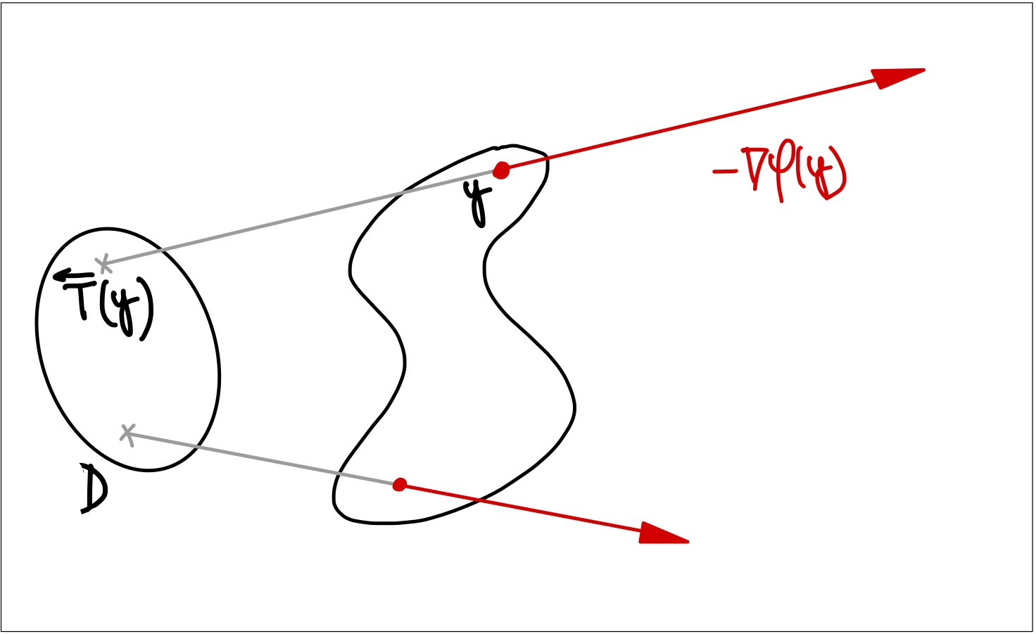
(a) Matter outside $D$

(b) Matter inside $D$

Figure 4. The force field depends on $D$

Polar factorization

The last ingredient to be introduced for a geometric interpretation of MAG  is Brenier’s polar factorization theorem [7]. During this subsection, $\lambda$ is any absolutely continuous probability measure on $\mathbb{R}^{d}$ satisfying $\int_{\mathbb{R}^{d}}|x|^{2}\,\lambda(dx)<\infty.$ The polar factorization theorem states that for any measurable mapping $\mathsf{y}:D\subset\mathbb{R}^{d}\to\mathbb{R}^{d}$ in

$$H:=L^{2}_{\mathbb{R}^{d}}(D,\lambda),$$

i.e. verifying $\|\mathsf{y}\|_{H}^{2}:=\int_{D}|\mathsf{y}(x)|^{2}\,\lambda(dx)<\infty,$ and such that the probability measure

$$\mu:=\mathsf{y}_{\#}\lambda$$

is also absolutely continuous, we have

$$\overleftarrow{T}\circ\mathsf{y}=\operatorname{proj}_{S}(\mathsf{y}),$$ (2.10)

where $\overleftarrow{T}$ is the optimal transport map from $\mu$ to $\lambda,$ and $\operatorname{proj}_{S}:H\to H$ is the orthogonal projection in the Hilbert space $H$ onto the subset

$$S:=\left\{\mathsf{x}\in H:\mathsf{x}_{\#}\lambda=\lambda\right\}$$

of all $\lambda$-preserving maps.

From now on, elements in $H$ will be written with bold letters. Note that

$$\|\mathsf{x}\|_{H}^{2}=\int_{D}|\mathsf{x}(x)|^{2}\,\lambda(dx)=\int_{D}|x|^{2}\,\mathsf{x}_{\#}\lambda(dx)=\int_{D}|x|^{2}\,\lambda(dx)=:r^{2}<\infty,\quad\forall\mathsf{x}\in S.$$ (2.11)

Hence, $S$ is a subset of a sphere; in particular it is not convex. The uniqueness of the projection of $\mathsf{y}$ on $S$, which is implied by the assumed absolute continuity of $\mu,$ is part the statement. This theorem is often expressed the reverse way:

$$\mathsf{y}={\overrightarrow{T}}\circ\operatorname{proj}_{S}(\mathsf{y}),$$

where ${\overrightarrow{T}}=(\overleftarrow{T})^{-1}$ is the optimal transport map from $\lambda$ to $\mu.$ It is worth seeing $\operatorname{proj}_{S}(\mathsf{y})$ as a type of permutation preserving $\lambda$ primer to the least cost mapping ${\overrightarrow{T}}.$

Geometric expression of MAG

In view of (1.1), (2.8) and (2.10), the collection of mappings $(\mathsf{y}_{t};t\geq 0)$ in $H$ is driven by MAG if

$$\ddot{\mathsf{y}}_{t}=\mathsf{y}_{t}-\operatorname{proj}_{S}(\mathsf{y}_{t}),\quad 0\leq t<t_{*}.$$ (2.12)

It is a detailed description of the evolution of the infinite particle system $(\mathsf{y}_{t}(x);x\in D)_{0\leq t<t_{*}}.$ In particular it gives the evolution of the fluid density $\mu_{t}:=(\mathsf{y}_{t})_{\#}\lambda.$

Concentration of matter

However, for (2.12) to be valid it is necessary that $\mu_{t}$ is absolutely continuous to ensure that $\mathsf{y}_{t}$ admits a unique projection on $S.$ Considering the converse of this implication, one sees that as soon as $\mathsf{y}_{t}$ has several projections on $S$, the matter distribution $\mu_{t}$ becomes singular with respect to Lebesgue measure. This appearance of singularities should be interpreted as concentration of matter. As $S$ is non-convex, this happens as a rule.
Choosing one candidate $\widehat{\operatorname{proj}}_{S}(\mathsf{y}_{t})$ as a function of the whole set $\operatorname{Proj}_{S}(\mathsf{y}_{t})$ of all the orthogonal projections of $\mathsf{y}_{t}$ on $S,$ determines the dynamics when concentration of matter occurs. A natural one is

$$\widehat{\operatorname{proj}}_{S}(\mathsf{y}):=\operatorname{proj}_{S(\mathsf{y})}(\mathsf{y})$$ (2.13)

where $S(\mathsf{y}):=\operatorname{cl}\operatorname{cv}(\operatorname{Proj}_{S}(\mathsf{y}))$ is the closed convex hull of $\operatorname{Proj}_{S}(\mathsf{y}).$ For a justification of this choice, see the appendix section.

Definition 2.14 (MAG dynamics allowing for matter concentration, [8]).

MAG dynamics described at Definition 2.6 is only valid for an absolutely continuous distribution of matter $\mu_{t}.$ In view of (2.12), an extension allowing for matter concentration is

$$\ddot{\mathsf{y}}_{t}=\mathsf{y}_{t}-\widehat{\operatorname{proj}}_{S}(\mathsf{y}_{t})\in H,\quad t\geq 0.$$ (2.15)

Remarks 2.16.

1. Because of the introduction of the extension $\widehat{\operatorname{proj}}_{S}$ of $\operatorname{proj}_{S}$ when $\operatorname{Proj}_{S}$ contains several points, this definition allows for mass concentration: time $t$ goes beyond $t_{*}$.

2. It depends on the choice of the extension $\widehat{\operatorname{proj}}_{S}$ of $\operatorname{proj}_{S}.$

3. Later, it will be convienient to work with action functionals, rather than with their Euler-Lagrange solutions. One must be aware that the connection between (2.15) and the natural candidate (2.21) below for a corresponding action functional is not fully established, see Remark 2.22-(b).

Action functional

A short reminder about action functionals and their connection with the equations of motion is proposed at Appendix B.

In [8], it is emphasized that the function

$$\Phi(\mathsf{y}):=\inf_{\mathsf{x}\in S}\|\mathsf{y}-\mathsf{x}\|_{H}^{2}/2=\|\mathsf{y}\|_{H}^{2}/2-\Pi_{S}(\mathsf{y})+r^{2}/2,\quad\mathsf{y}\in H,$$

where

$$\mathsf{y}\mapsto\Pi_{S}(\mathsf{y}):=\sup_{\mathsf{x}\in S}\left\langle\mathsf{x},\mathsf{y}\right\rangle_{H},$$

is differentiable at any $\mathsf{y}$ which admits a unique projection on $S$. Moreover, for any such "nice" $\mathsf{y}$,

$$\nabla\Phi(\mathsf{y})=\mathsf{y}-\nabla\Pi_{S}(\mathsf{y})=\mathsf{y}-\operatorname{proj}_{S}(\mathsf{y}).$$ (2.17)

This implies

$$\Phi(\mathsf{y})=\|\nabla\Phi(\mathsf{y})\|_{H}^{2}/2,$$

and also that a Lagrangian associated to Newton’s equation (2.12) is

$$\|\dot{\mathsf{y}}\|_{H}^{2}/2+\Phi(\mathsf{y}).$$ (2.18)

Plugging the last but one identity into the last one, the Lagrangian becomes $\|\dot{\mathsf{y}}\|_{H}^{2}/2+\Phi(\mathsf{y})=\|\dot{\mathsf{y}}\|_{H}^{2}/2+\|\nabla\Phi(\mathsf{y})\|_{H}^{2}/2=\|\dot{\mathsf{y}}-\nabla\Phi(\mathsf{y})\|_{H}^{2}/2+\langle\nabla\Phi(\mathsf{y}),\dot{\mathsf{y}}\rangle_{H}.$ As $\langle\nabla\Phi(\mathsf{y}),\dot{\mathsf{y}}\rangle_{H}$ is a null Lagrangian (because $\displaystyle{\langle\nabla\Phi(\mathsf{y}_{t}),\dot{\mathsf{y}}_{t}\rangle_{H}=\frac{d}{dt}\Phi(\mathsf{y}_{t})}$ is a total derivative), one can choose the alternate Lagrangian $\|\dot{\mathsf{y}}-\nabla\Phi(\mathsf{y})\|_{H}^{2}/2$ without modifying the dynamics. Its leads to the action functional

$$\int_{t_{0}}^{t_{1}}\scalebox{1.2}{$\frac{1}{2}$}\|\dot{\mathsf{y}}_{t}-\nabla\Phi(\mathsf{y}_{t})\|_{H}^{2}\ dt=\int_{t_{0}}^{t_{1}}\scalebox{1.2}{$\frac{1}{2}$}\|\dot{\mathsf{y}}_{t}-\mathsf{y}_{t}+\operatorname{proj}_{S}(\mathsf{y}_{t})\|_{H}^{2}\ dt,$$ (2.19)

which becomes meaningless as soon as $t_{1}$ is larger than the first time $t^{*}$ when the set $\operatorname{Proj}_{S}(\mathsf{y}_{t^{*}})$ contains at least two elements. Finally, Brenier proposes the following

Definition 2.20 (Action functional of MAG pushed by $D$, [8]).

It is

$$\int_{t_{0}}^{t_{1}}\scalebox{1.2}{$\frac{1}{2}$}\|\dot{\mathsf{y}}_{t}-\widehat{\nabla}\Phi(\mathsf{y}_{t})\|_{H}^{2}\ dt=\int_{t_{0}}^{t_{1}}\scalebox{1.2}{$\frac{1}{2}$}\|\dot{\mathsf{y}}_{t}-\mathsf{y}_{t}+\widehat{\operatorname{proj}}_{S}(\mathsf{y}_{t})\|_{H}^{2}\ dt,$$ (2.21)

the extended gradient $\widehat{\nabla}\Phi(\mathsf{y})$ being defined by

$$\widehat{\nabla}\Phi(\mathsf{y}):=\mathsf{y}-\widehat{\nabla}\Pi_{S}(\mathsf{y})=\mathsf{y}-\widehat{\operatorname{proj}}_{S}(\mathsf{y})$$

where $\widehat{\nabla}\Pi_{S}(\mathsf{y})$ is the (unique) element with minimal norm in the subdifferential $\partial\Pi_{S}(\mathsf{y})$ of the convex function $\Pi_{S}$.

Remarks 2.22.

1. In view of (2.18), another candidate for an action functional of MAG is

   $$\|\dot{\mathsf{y}}\|_{H}^{2}/2+\widehat{\Phi}(\mathsf{y}).$$

   Unlike this action, the action (2.21) looks like a Freidlin-Wentzell large deviation rate function. This will be exploited at Section 3, see (3.7).

2. It is noticed in [8] that it is not clear that these action functionals are equivalent and that one of them admits (2.15) as its Euler-Lagrange equation.

3. It happens that $\widehat{\nabla}\Pi_{S}(\mathsf{y})=\widehat{\operatorname{proj}}_{S}(\mathsf{y}),$ as defined at (2.13). See Proposition C.6.

Extension to a discrete source measure

Let us replace the normalized volume measure $\lambda$ of some set $D\in\mathbb{R}^{d}$ with a strictly positive Lebesgue volume, see (2.5), by the normalized counting measure

$$\lambda^{(k)}:=\frac{1}{k}\sum_{1\leq j\leq k}\delta_{x_{j}}$$ (2.23)

on some finite set $D^{(k)}:=\{x_{1},\dots,x_{k}\}\subset\mathbb{R}^{d}.$ Any mapping $\mathsf{y}:D^{(k)}\to\mathbb{R}^{d}$ is encoded by the vector $\mathsf{y}:=(\mathsf{y}(x_{1}),\dots,\mathsf{y}(x_{k}))\in(\mathbb{R}^{d})^{k}$ whose squared norm in the Hilbert space $H:=L^{2}_{\mathbb{R}^{d}}(\lambda^{(k)})$ is

$$\|\mathsf{y}\|_{H}^{2}=k^{-1}\sum_{1\leq j\leq k}|\mathsf{y}(x_{j})|^{2}=k^{-1}\|\mathsf{y}\|^{2}$$

where $|\,\begin{picture}(-1.0,1.0)(-1.0,-3.0)\circle*{3.0}\end{picture}\ |$ and $\|\,\begin{picture}(-1.0,1.0)(-1.0,-3.0)\circle*{3.0}\end{picture}\ \|$ are respectively the Euclidean norms on $\mathbb{R}^{d}$ and $(\mathbb{R}^{d})^{k}.$ Hence,

$$H\simeq(\mathbb{R}^{d})^{k}.$$

Definition 2.24 ($k$-mapping).

When the source measure is the discrete measure $\lambda^{(k)}$, we call any application $\mathsf{y}:D^{(k)}\to\mathbb{R}^{d}$ in $H$ a $k$-mapping.

For the ease of notation, we shall write $\mathbb{R}^{dk}$ instead of $(\mathbb{R}^{d})^{k}$, but one should keep in mind the structure of $(\mathbb{R}^{d})^{k}$. Also, keeping our convention of writing elements of $H$ with bold letters, any $k$-mapping will also be written this way.
The set $S$ of all $k$-mappings preserving $\lambda^{(k)}$ is

$$S=\{\mathsf{x}^{\sigma};\sigma\in\mathcal{S}\}$$ (2.25)

where $\mathcal{S}$ is the set of all permutations of $k$ elements and

$$\mathsf{x}^{\sigma}:=(x_{\sigma(1)},\dots,x_{\sigma(k)})\in H,\qquad\sigma\in\mathcal{S}.$$

Brenier proposed in [9] to extend Definition 2.20 to this semi-discrete setting which is natural to implement numerical simulations [25].

Definition 2.26 (Action functional of MAG pushed by $\{x_{1},\dots,x_{k}\}$, [9]).

It is still (2.21) as in Definition 2.20, but $H\simeq(\mathbb{R}^{d})^{k}$ and $S$ is given by (2.25).

This definition is the basis for the definitions of new action functionals we will work with in the rest of the article, see (4.18) and Definitions 4.7, 5.9 and 5.13. At present time, it is only justified by analogy with Definition 2.20. Its effectiveness in the numerical simulations suggests that one should recover (2.21) by letting $k$ tend to infinity and preparing $\lambda^{(k)}$ such that $\lim_{k\to\infty}\lambda^{(k)}=\mathbf{1}_{D}\,\mathrm{Leb}.$

3. MAG. Particle system

This section is aimed at giving a presentation of a random particle system, see (3.7) below, introduced by Ambrosio, Baradat and Brenier in [2] whose dynamics is related to the action functional of MAG pushed by $\{x_{1},\dots,x_{k}\}$ introduced at Definition 2.26, see (3.12) below.

Let us introduce the following stochastic differential equation in the set $\mathbb{R}^{dk}$ of $k$-mappings

$$\mathsf{X}^{\epsilon}_{s}=\mathsf{X}_{0}+\sqrt{\epsilon}\,\mathsf{B}_{s},\quad s\geq 0,$$ (3.1)

where $\mathsf{B}$ is a standard Brownian motion in $\mathbb{R}^{dk}$ starting from zero, $\epsilon>0$ is a fluctuation parameter which is intended to tend to zero, and the law of the initial position $\mathsf{X}_{0}$ in $\mathbb{R}^{dk}$ is

$$r_{0}:=\textrm{Law}(\mathsf{X}_{0})=\frac{1}{k!}\sum_{\sigma\in\mathcal{S}}\delta_{\mathsf{x}^{\sigma}}.$$ (3.2)

The process $\mathsf{X}^{\epsilon}_{s}=(\mathsf{X}^{\epsilon,1}_{s},\dots,\mathsf{X}^{\epsilon,k}_{s})$ describes a cloud of $k$ indistinguishable Brownian particles in $\mathbb{R}^{d}$ starting from $\{x_{1},\dots,x_{k}\}$; indistinguishability being a direct consequence of the choice (3.2) of the initial law. It is a random path of $k$-mappings. The $j$-th coordinate $\mathsf{X}^{\epsilon,j}$ is the path of the $j$-th particle starting from the $j$-th random draw without replacement from the set $\{x_{1},\dots,x_{k}\}.$ Remark that although the coordinates $\mathsf{X}^{\epsilon,j},$ $1\leq j\leq k,$ are correlated, they share the same law with initial distribution $\lambda^{(k)},$ see (2.23).

For any $s>0$, the law of $\mathsf{X}^{\epsilon}_{s}$ is the following mixture of Gaussian measures in $\mathbb{R}^{dk}$ with means $\mathsf{x}^{\sigma}$ and covariance matrices $\epsilon s\,\mathbb{I}:$

$$r^{\epsilon}_{s}(d\mathsf{x})=\frac{1}{k!}\sum_{\sigma\in\mathcal{S}}(2\pi\epsilon s)^{-dk/2}\exp\left(-\frac{\|\mathsf{x}-\mathsf{x}^{\sigma}\|^{2}}{2\epsilon s}\right)\,d\mathsf{z}.$$ (3.3)

It solves the heat equation

$$\partial_{s}r^{\epsilon}=\epsilon\Delta r^{\epsilon}/2$$ (3.4)

which rewrites as the continuity equation

$$\partial_{s}r^{\epsilon}+\nabla\!\cdot\!(r^{\epsilon}{\dot{\mathsf{r}}^{\epsilon}})=0$$

with the current velocity field ${\dot{\mathsf{r}}^{\epsilon}}$ on $\mathbb{R}^{dk}$ of the diffusion process $\mathsf{X}^{\epsilon}$ defined for any $s>0$ and any $\mathsf{x}\in\mathbb{R}^{dk}$ by

$$\begin{split}{\dot{\mathsf{r}}^{\epsilon}}_{s}(\mathsf{x})&=-\epsilon\nabla\log\sqrt{r^{\epsilon}_{s}}(\mathsf{x})\\ &=-\frac{\epsilon\nabla r^{\epsilon}_{s}}{2r^{\epsilon}_{s}}(\mathsf{x})=\frac{\sum_{\sigma\in\mathcal{S}}(\mathsf{x}-\mathsf{x}^{\sigma})\exp\big{(}-{\|\mathsf{x}-\mathsf{x}^{\sigma}\|^{2}}/(2\epsilon s)\big{)}}{2s\sum_{\sigma\in\mathcal{S}}\exp\big{(}-{\|\mathsf{x}-\mathsf{x}^{\sigma}\|^{2}}/(2\epsilon s)\big{)}}\\ &=\frac{1}{2s}\left(\mathsf{x}-\frac{\sum_{\sigma\in\mathcal{S}}\mathsf{x}^{\sigma}\exp\big{(}-{\|\mathsf{x}-\mathsf{x}^{\sigma}\|^{2}}/(2\epsilon s)\big{)}}{\sum_{\sigma\in\mathcal{S}}\exp\big{(}-{\|\mathsf{x}-\mathsf{x}^{\sigma}\|^{2}}/(2\epsilon s)\big{)}}\right).\end{split}$$ (3.5)

Letting $\epsilon$ tend to zero, we see with the Laplace principle that for any $s>0,$ $\lim_{\epsilon\rightarrow 0}{\dot{\mathsf{r}}^{\epsilon}}_{s}(\mathsf{x})=(2s)^{-1}(\mathsf{x}-\mathsf{x}^{\sigma(\mathsf{x})})$ where $\mathsf{x}^{\sigma(\mathsf{x})}$ is the closest point from $\mathsf{x}$ among all the $\mathsf{x}^{\sigma}$ in $S,$ provided that this closest point is unique. In view of (2.25), under this uniqueness assumption this means that

$$\lim_{\epsilon\rightarrow 0}{\dot{\mathsf{r}}^{\epsilon}}_{s}(\mathsf{x})=\frac{\mathsf{x}-\operatorname{proj}_{S}(\mathsf{x})}{2s},$$ (3.6)

a formula similar to the right hand side of equation (2.12). Getting rid of the factor $(2s)^{-1}$ will be a matter of change of time, see the parameter setting 3.10 below.

Since the action functional (2.19) can be read as some large deviation rate function, it is proposed in [2] to consider the stochastic differential equation in $\mathbb{R}^{dk}$

$$d\mathsf{Z}^{\epsilon,\eta}_{s}={\dot{\mathsf{r}}^{\epsilon}}_{s}(\mathsf{Z}^{\epsilon,\eta}_{s})\,ds+\sqrt{\eta k^{2}\kappa_{s}^{-1}}\,d\mathsf{W}_{s},\quad 0<s_{0}\leq s\leq s_{1},$$ (3.7)

where ${\dot{\mathsf{r}}^{\epsilon}}$ is the current velocity (3.5), $s\mapsto\kappa_{s}$ is a positive function, $\eta>0$ is a parameter intended to decrease to zero and $\mathsf{W}$ is a standard Brownian motion on $\mathbb{R}^{dk}$. The Freidlin-Wentzell large deviation principle roughly states that, for any fixed $\epsilon>0$ and any initial state $\mathsf{x}_{o}$ in $\mathbb{R}^{dk},$ when $\eta$ tends to zero

$$\mathrm{Proba}(\mathsf{Z}^{\epsilon,\eta}\in\,\begin{picture}(-1.0,1.0)(-1.0,-3.0)\circle*{3.0}\end{picture}\ \mid\mathsf{Z}^{\epsilon,\eta}_{s_{0}}=\mathsf{z}_{o})\underset{\eta\to 0}{\asymp}\exp\left(-\eta^{-1}\ \inf_{\mathsf{z}\in\bullet,\mathsf{z}(s_{0})=\mathsf{z}_{o}}\widetilde{A}^{\epsilon}(\mathsf{z})\right)$$

with the large deviation rate function

$$\widetilde{A}^{\epsilon}[(\mathsf{z}_{s})_{s_{0}\leq s\leq s_{1}}]=\int_{s_{0}}^{s_{1}}\scalebox{1.2}{$\frac{1}{2}$}\|\dot{\mathsf{z}}_{s}-{\dot{\mathsf{r}}^{\epsilon}}_{s}(\mathsf{z}_{s})\|_{H}^{2}\,\kappa_{s}\,ds$$ (3.8)

where $(\mathsf{z}_{s})_{s_{0}\leq s\leq s_{1}}$ stands for a generic absolutely continuous path taking its values in $\mathbb{R}^{dk}$. Remember that $\|\,\begin{picture}(-1.0,1.0)(-1.0,-3.0)\circle*{3.0}\end{picture}\ \|_{H}=k^{-1}\|\,\begin{picture}(-1.0,1.0)(-1.0,-3.0)\circle*{3.0}\end{picture}\ \|_{\mathbb{R}^{dk}}$ and also that the factor $k$ is part of the diffusion coeffective in (3.7). It is proved in [2], see also [1], that

$$\Gamma\textrm{-}\lim_{\epsilon\to 0}\widetilde{A}^{\epsilon}\big{[}(\mathsf{z}_{s})_{s_{0}\leq s\leq s_{1}})\big{]}=\int_{s_{0}}^{s_{1}}\scalebox{1.2}{$\frac{1}{2}$}\Big{\|}\dot{\mathsf{z}}_{s}-\frac{\mathsf{z}_{s}-\widehat{\operatorname{proj}}_{S}(\mathsf{z}_{s})}{2s}\Big{\|}_{H}^{2}\,\kappa_{s}\,ds,$$ (3.9)

with $\widehat{\operatorname{proj}}_{S}$ defined at (2.13). Compare with (3.6).
It is easily seen (see (5.8) below for details) that applying the following

Parameter setting 3.10.

• choose $\kappa_{s}=2s$,

• change time: $s=e^{2t},$

and denoting $\mathsf{y}_{t}:=\mathsf{z}_{e^{2t}}$, the right-hand side of (3.8) becomes

$$A^{\epsilon}\big{[}(\mathsf{y}_{t})_{t_{0}\leq t\leq t_{1}})\big{]}:=\int_{t_{0}}^{t_{1}}\scalebox{1.2}{$\frac{1}{2}$}\Big{\|}\dot{\mathsf{y}}_{t}-\mathsf{y}_{t}+\frac{\sum_{\sigma\in\mathcal{S}}\mathsf{x}^{\sigma}\exp\big{(}-{\|\mathsf{y}_{t}-\mathsf{x}^{\sigma}\|^{2}}/(2\epsilon e^{2t})\big{)}}{\sum_{\sigma\in\mathcal{S}}\exp\big{(}-{\|\mathsf{y}_{t}-\mathsf{x}^{\sigma}\|^{2}}/(2\epsilon e^{2t})\big{)}}\Big{\|}_{H}^{2}\,dt,$$ (3.11)

where $t_{0}=\log\sqrt{s_{0}}$ and $t_{1}=\log\sqrt{s_{1}}$ and the $\Gamma$-limit (3.9) becomes

$$\Gamma\textrm{-}\lim_{\epsilon\to 0}A^{\epsilon}\big{[}(\mathsf{y}_{t})_{t_{0}\leq t\leq t_{1}})\big{]}=\int_{t_{0}}^{t_{1}}\scalebox{1.2}{$\frac{1}{2}$}\|\dot{\mathsf{y}}_{t}-\mathsf{y}_{t}+\widehat{\operatorname{proj}}_{S}(\mathsf{y}_{t})\|_{H}^{2}\,dt.$$ (3.12)

As desired, it is MAG’s action (2.21). Remark that the appearance of the hat upon $\operatorname{proj}_{S}$ is a consequence of the $\Gamma$-limit.

Definition 3.13 (Action of $\epsilon$-MAG pushed by $\{x_{1},\dots,x_{k}\}$).

The functional $A^{\epsilon}$ defined at (3.11) is the action of $\epsilon$-MAG pushed by $\{x_{1},\dots,x_{k}\}$.
Its $s$-version is $\widetilde{A}^{\epsilon}$ defined by (3.8).

Remarks

1. In [2], the $k$-mapping-valued stochastic process (3.7) is interpreted as surfing the heat wave, pointing out some analogy with de Broglie’s pilot wave theory in quantum physics.

2. Let us quote a sentence from [2]: “Unexpectedly, the action (3.12) is exactly the one previously suggested by the third author (Brenier) in [8] to include dissipative phenomena (such as sticky collisions in one space dimension) in the Monge-Ampère gravitational model!” The physical interpretation of the intriguing particle system (3.7) is also unclear to us at first sight, while its connection with MAG seems tight enough to think that it might not be incidental.

The significant feature of the stochastic differential equation (3.7) is that the forward velocity of $\mathsf{Z}^{\epsilon,\eta}$: the drift field ${\dot{\mathsf{r}}^{\epsilon}}$, is the current velocity of someone else, namely $\mathsf{Z}^{\epsilon}$. How to give a meaning to this substitution? One purpose of this article is to propose at Section 9 alternate Brownian particle systems with a clearer physical meaning.

In order to proceed in this direction, we need to extend MAG from mappings $\mathsf{y}$ to fluids.

4. MAG for a fluid

We look at the evolution of a self-gravitating fluid in $\mathbb{R}^{d}$ governed by a MAG force field. This section only deals with MAG: we drop $\epsilon$-MAG for a while.

Sections 2 and 3 were dedicated to the flow of mappings $t\mapsto\mathsf{y}_{t}=(\mathsf{y}_{t}(x))_{x\in D},$ keeping track of the source element $x\in D.$ This was necessary to obtain a representation in terms of optimal transport. However, fluid particles being indistinguishable, we do not observe the detail of the mapping $\mathsf{y}_{t},$ but only the profile

$$\mu_{t}:=(\mathsf{y}_{t})_{\#}\lambda\in\mathrm{P}(\mathbb{R}^{d})$$ (4.1)

of positions at time $t$. The following term is part of the integrand of the action (2.21):

$$\|\dot{\mathsf{y}}_{t}-\{\mathsf{y}_{t}-\widehat{\operatorname{proj}}_{S}(\mathsf{y}_{t})\}\|_{H}^{2}=\int_{D}|\dot{\mathsf{y}}_{t}(x)-\{\mathsf{y}_{t}(x)-[\widehat{\operatorname{proj}}_{S}(\mathsf{y}_{t})](x)\}|^{2}\,\lambda(dx).$$

Properties 4.2.

Suppose that there exist a vector field $v_{t}(y)$ and a map $\widehat{T}(\mu,y)$ such that for any $x$ in $D$,

$$\bullet\quad \dot{\mathsf{y}}_{t}(x)=v_{t}\big{(}\mathsf{y}_{t}(x)\big{)}\in\mathbb{R}^{d},$$ (4.3)

$$\bullet\quad [\widehat{\operatorname{proj}}_{S}(\mathsf{y}_{t})](x)=\widehat{T}\big{(}{\mu_{t}},\mathsf{y}_{t}(x)\big{)}\in\mathbb{R}^{d}\quad\textrm{where}\quad\mu_{t}:=(\mathsf{y}_{t})_{\#}\lambda.$$ (4.4)

Then, (2.21) writes as

$$\begin{split}\int_{t_{0}}^{t_{1}}\scalebox{1.2}{$\frac{1}{2}$}\|\dot{\mathsf{y}}_{t}-\{\mathsf{y}_{t}&-\widehat{\operatorname{proj}}_{S}(\mathsf{y}_{t})\}\|_{H}^{2}\,dt\\ &=\int_{D\times[t_{0},t_{1}]}\scalebox{1.2}{$\frac{1}{2}$}|v_{t}\big{(}\mathsf{y}_{t}(x)\big{)}-\{\mathsf{y}_{t}(x)-\widehat{T}\big{(}{\mu_{t}},\mathsf{y}_{t}(x)\big{)}\}|^{2}\,\lambda(dx)dt\\ &=\int_{\mathbb{R}^{d}\times[t_{0},t_{1}]}\scalebox{1.2}{$\frac{1}{2}$}|v_{t}(y)-[y-\widehat{T}({\mu_{t}},y)]|^{2}\,\mu_{t}(dy)dt\\ &=\int_{t_{0}}^{t_{1}}\scalebox{1.2}{$\frac{1}{2}$}\left\langle|v_{t}-(\mathrm{Id}-\widehat{T}_{\mu_{t}})|^{2},\mu_{t}\right\rangle\,dt=\int_{t_{0}}^{t_{1}}\scalebox{1.2}{$\frac{1}{2}$}\|v_{t}-(\mathrm{Id}-\widehat{T}_{\mu_{t}})\|^{2}_{\mu_{t}}\,dt,\end{split}$$ (4.5)

where last but one equality is simply a change of notation: $\left\langle f,\mu\right\rangle:=\int_{\mathbb{R}^{d}}f\,d\mu$, and $\|\,\begin{picture}(-1.0,1.0)(-1.0,-3.0)\circle*{3.0}\end{picture}\ \|_{\mu}$ is a shorthand for $\|\,\begin{picture}(-1.0,1.0)(-1.0,-3.0)\circle*{3.0}\end{picture}\ \|_{L^{2}_{\mathbb{R}^{d}}(\mu)}$. By (4.3), $v_{t}$ is the velocity field of the fluid with density $\mu_{t}$. Hence, the continuity equation

$$\partial_{t}\mu_{t}+\nabla\!\cdot\!(\mu_{t}v_{t})=0$$ (4.6)

is satisfied in a weak sense. Although this notation suggests that $\mu_{t}$ should be absolutely continuous, no such hypothesis is done at Proposition 4.11 below: the weak formulation (4.12) is valid for any probability measure $\mu_{t}$.

Dropping the requirement (4.1) that the density profile is represented by $\mu_{t}=(\mathsf{y}_{t})_{\#}\lambda$ for some flow of mappings $(\mathsf{y}_{t})_{t_{0}\leq t\leq t_{1}},$ the identity (4.5) suggests the following extension to a fluid of the definition of Monge-Ampère gravitation.

Definition 4.7 (MAG’s action for a fluid pushed by $\lambda$).

Let $\lambda$ be any probability measure on $D\subset\mathbb{R}^{d}$. A least action principle for a MAG  self-gravitating fluid pushed by $\lambda$ is

$$\inf_{(\mu,v)}\int_{t_{0}}^{t_{1}}\scalebox{1.2}{$\frac{1}{2}$}\|v_{t}-(\mathrm{Id}-\widehat{T}_{\mu_{t}})\|^{2}_{\mu_{t}}\,dt$$ (4.8)

where

1. the infimum runs through all $(\mu,v)$ satisfying the continuity equation (4.6) in the weak sense (4.12), and such that the endpoint marginals $\mu_{t_{0}}$ and $\mu_{t_{1}}$ are prescribed,

2. $\widehat{T}_{\mu}$ is the optimal map $\overleftarrow{T}_{\mu}$ transporting $\mu$ to $\lambda,$ if the Monge transport problem admits a unique solution, or some extension of it if uniqueness fails, see Remark 4.9-(c) below.

This model depends on the choices of the measure $\lambda$ and the extension $\widehat{T}$ of $\overleftarrow{T}.$

Remarks 4.9.

Clearly, its physical adequateness depends on the fulfillment of Properties 4.2. Let us comment on them.

1. As far as one is interested in the evolution of the density $\mu_{t}$ forgetting the details of the mapping $\mathsf{y}_{t},$ property (4.3) is justified by Proposition 4.11 below.

2. Let us have a look at property (4.4). As long as $\mu_{t}$ remains absolutely continuous, for any $x\in D,$ the $x$-th component $[\widehat{\operatorname{proj}}_{S}(\mathsf{y}_{t})](x)\in\mathbb{R}^{d}$ of $\widehat{\operatorname{proj}}_{S}(\mathsf{y}_{t})$ only depends on $\mu_{t}$ and the position $\mathsf{y}_{t}(x)$ of the $x$-th particle in $\mathbb{R}^{d}.$ Indeed, in this situation $\operatorname{Proj}_{S}(\mathsf{y}_{t})$ contains the single element $\operatorname{proj}_{S}(\mathsf{y}_{t})=\overleftarrow{T}_{\mu_{t}}\circ\mathsf{y}_{t}$ where by (2.3)

   $$\overleftarrow{T}_{\mu_{t}}=\nabla\theta_{t}$$ (4.10)

   is the optimal transport map from the absolutely continuous measure $\mu_{t}$ to the measure $\lambda,$ in which case $[\widehat{\operatorname{proj}}_{S}(\mathsf{y}_{t})](x)=[\operatorname{proj}_{S}(\mathsf{y}_{t})](x)=\overleftarrow{T}_{\mu_{t}}(\mathsf{y}_{t}(x)).$

3. We think that it is physically reasonable to assume that property (4.4) still holds when $\mu_{t}$ fails to be absolutely continuous. We think that a privileged model should consist of replacing $\overleftarrow{T}_{\mu_{t}}(y)$ by the orthogonal projection in $\mathbb{R}^{d}$ of $y$ on the closed convex hull of the subset $\cup_{\pi_{\ mu_{t}}}\operatorname{supp}\pi_{\mu_{t}}(\,\begin{picture}(-1.0,1.0)(-1.0,-3.0)\circle*{3.0}\end{picture}\ \mid y)$, where the union runs through the collection $\{\pi_{\mu_{t}}\}$ of all solutions of the Monge-Kantorovich optimal transport problem from $\mu_{t}$ to $\lambda,$ and $\operatorname{supp}\pi_{\mu_{t}}(\,\begin{picture}(-1.0,1.0)(-1.0,-3.0)\circle*{3.0}\end{picture}\ \mid y)$ stands for the support of the optimal plan $\pi_{\mu_{t}}$ conditioned by the knowledge of the source location $y.$

Let us recall the following standard result justifying Remark 4.9-(a).

Proposition 4.11.

Suppose that the (normalized) density $\mu_{t}=(Y_{t})_{\#}P$ is the time marginal at time $t$ of some path measure $P\in\mathrm{P}(\Omega)$ which is supported by absolutely continuous sample paths, i.e.

$$dY_{t}=\dot{Y}_{t}\,dt,\quad P\textrm{-}\mathrm{a.s.},$$

where $(Y_{t})_{t_{0}\leq t\leq t_{1}}$ stands for the canonical process on the path space

$$\Omega:=C([t_{0},t_{1}],\mathbb{R}^{d})$$

and $\dot{Y}_{t}$ is some random vector, possibly depending (a priori) on the whole history of the path and satisfying

$$E_{P}\int_{t_{0}}^{t_{1}}|\dot{Y}_{t}|^{2}\,dt<\infty.$$

Then, there exists some measurable vector field $v_{t}(y)$ such that for almost all $t$, $v_{t}$ belongs to the closure $H^{-1}_{\mathbb{R}^{d}}(\mu_{t})$ in $L^{2}_{\mathbb{R}^{d}}(\mu_{t})$ of the space $\left\{\nabla u;u\in C^{1}_{c}(\mathbb{R}^{d})\right\}$ of regular gradient vector fields,

$$\int_{\mathbb{R}^{d}\times[t_{0},t_{1}]}|v_{t}(y)|^{2}\,\mu_{t}(dy)dt<\infty,$$

and the continuity equation (4.6) holds in the following weak sense: For any function $f$ in $C^{1}_{c}(\mathbb{R}^{d})$ and any $t_{0}\leq t_{*}\leq t_{1},$

$$\int_{\mathbb{R}^{d}}f \,d\mu_{t_{*}}-\int_{\mathbb{R}^{d}}f\,d\mu_{t_{0}}=\int_{\mathbb{R}^{d}\times[t_{0},t_{*}]}\nabla f(y)\!\cdot\!v_{t}(y)\,\mu_{t}(dy)dt.$$ (4.12)

Proof.

Take any function $g$ in $C^{1,1}_{c}(\mathbb{R}^{d}\times[t_{0},t_{*}])$ with $t_{0}\leq t_{*}\leq t_{1}.$ Then,

$$\int_{\mathbb{R}^{d}}g_{t_{*}} \,d\mu_{t_{*}}-\int_{\mathbb{R}^{d}}g_{t_{0}}\,d\mu_{t_{0}}=E_{P}\int_{t_{0}}^{t_{*}}[\partial_{t}g_{t}(Y_{t})+\nabla g_{t}(Y_{t})\!\cdot\!\dot{Y}_{t}]\,dt$$

$$=E_{\bar{P}}(\partial_{t}g(\tau,Y_{\tau})+\nabla g_{\tau}(Y_{\tau})\!\cdot\!\dot{Y}_{\tau})=E_{\bar{P}}E_{\bar{P}}\big{[}\partial_{t}g(\tau,Y_{\tau})+\nabla g_{\tau}(Y_{\tau})\!\cdot\!\dot{Y}_{\tau}\mid(Y_{\tau},\tau)\big{]}$$

$$=E_{\bar{P}}\big{[}\partial_{t}g(\tau,Y_{\tau})+\nabla g_{\tau}(Y_{\tau})\!\cdot\!\tilde{v}_{\tau}(Y_{\tau})\big{]}=\int_{\mathbb{R}^{d}\times[t_{0},t_{*}]}\big{[}\partial_{t}g_{t}(y)+\nabla g_{t}(y)\!\cdot\!\tilde{v}_{t}(y)\big{]}\,\mu_{t}(dy)dt$$

$$=\int_{\mathbb{R}^{d}\times[t_{0},t_{*}]}\big{[}\partial_{t}g_{t}(y)+\nabla g_{t}(y)\!\cdot\!v_{t}(y)\big{]}\,\mu_{t}(dy)dt,\$$

where $\bar{P}(d\omega dt):=P(d\omega)dt$, the canonical time is $\tau$, $\tilde{v}_{t}(y):=E_{\bar{P}}\left(\dot{Y}_{\tau}\mid Y_{\tau}=y,\tau=t\right),$ and $v$ is the orthogonal projection in $L^{2}_{\mathbb{R}^{d}}(\mu_{t}(dy)dt)$ of $\tilde{v}$ on the closure of the space $\left\{\nabla g;g\in C^{1,1}_{c}(\mathbb{R}^{d}\times[t_{0},t_{*}])\right\}$. This implies (4.12) and the joint measurability of $(t,y)\mapsto v_{t}(y)$. ∎

From $\inf_{(\mu,u)}$ to $\inf_{(\mu)}$, Otto calculus

The basic insight of Otto calculus [29, 3, 33], is to interpret the velocity field $v_{t}\in H^{-1}_{\mathbb{R}^{d}}(\mu_{t})$ appearing at Proposition 4.11 as a tangent vector at $\mu_{t}$ in some Riemannian-like manifold $\mathrm{P}_{2}\subset\mathrm{P}(\mathbb{R}^{d})$, called the Otto-Wasserstein manifold. We denote this velocity by

$$\dot{\mu}_{t}:=v_{t}\in\mathrm{T}_{\mu_{t}}\mathrm{P}_{2}\subset H^{-1}_{\mathbb{R}^{d}}(\mu_{t})$$ (4.13)

where $\mathrm{T}_{\mu}\mathrm{P}_{2}$ stands for the tangent space of $\mathrm{P}_{2}$ at $\mu.$ In particular, the continuity equation (4.6) writes as

$$\partial_{t}\mu+\nabla\!\cdot\!(\mu\dot{\mu})=0.$$

We emphasize that the vertical variation $\partial_{t}\mu_{t}$ differs form the horizontal variation $\dot{\mu}_{t}.$
The relation between quadratic optimal transport and Otto calculus is best illustrated by the Benamou-Brenier formula

$$W_{2}^{2}(\alpha,\beta) \overset{(\textrm{i})}{=}\inf_{(\mu,u)}\int_{0}^{1}\Big{(}\int_{\mathbb{R}^{d}}|u_{t}(y)|^{2}\,\mu_{t}(dy)\Big{)}\,dt$$

$$\qquad\overset{(\textrm{ii})}{=}\inf_{(\mu)}\int_{0}^{1}\Big{(}\int_{\mathbb{R}^{d}}|\dot{\mu}_{t}(y)|^{2}\,\mu_{t}(dy)\Big{)}\,dt\overset{(\textrm{iii})}{=}\inf_{(\mu)}\int_{0}^{1}\|\dot{\mu}_{t}\|^{2}_{\mu_{t}}\,dt,$$

where $\alpha,\beta\in\mathrm{P}(\mathbb{R}^{d})$ and

$$W_{2}^{2}(\alpha,\beta):=\inf_{\pi}\int_{\mathbb{R}^{d}\times\mathbb{R}^{d}}|y-x|^{2}\,\pi(dxdy)$$

is the optimal quadratic transport cost from $\alpha$ to $\beta.$
Let us comment on these infimums:

1. in the expression $\inf_{\pi},$ $\pi\in\mathrm{P}(\mathbb{R}^{d}\times\mathbb{R}^{d})$ runs through all the couplings of $\alpha$ and $\beta,$ that is: $\pi(dx\times\mathbb{R}^{d})=\alpha(dx)$ and $\pi(\mathbb{R}^{d}\times dy)=\beta(dy);$

2. in the expression $\inf_{(\mu)},$ the infimum runs through all the paths $(\mu)=(\mu_{t})_{0\leq t\leq 1}$ in $\mathrm{P}(\mathbb{R}^{d})$ such that $\mu_{0}=\alpha$ and $\mu_{1}=\beta;$

3. in the expression $\inf_{(\mu,u)},$ the infimum runs through all the paths $(\mu,u)=(\mu_{t},u_{t})_{0\leq t\leq 1}$ where $\mu_{0}=\alpha$, $\mu_{1}=\beta$ and the $u_{t}$’s are vector fields such that the continuity equation $\partial_{t}\mu+\nabla\cdot(\mu u)=0$ holds in the weak sense.

Identity (i) is the Benamou-Brenier formula. Identity (ii) relies on Proposition 4.11 which states that one can replace $u_{t}$ in the continuity equation $\partial_{t}\mu+\nabla\cdot(\mu u)=0$ by $\dot{\mu}_{t}$ which, as an element of $H^{-1}_{\mathbb{R}^{d}}(\mu_{t}),$ minimizes $\int_{\mathbb{R}^{d}}|u_{t}|^{2}\,d\mu_{t}$ (Hilbertian projection onto $H^{-1}_{\mathbb{R}^{d}}(\mu_{t})$). The last equality (iii) directly follows from the notation

$$\|\dot{\mu}_{t}\|^{2}_{\mu_{t}}:=\int_{\mathbb{R}^{d}}|\dot{\mu}_{t}(y)|^{2}\,\mu_{t}(dy)$$ (4.14)

where $\|\dot{\mu}_{t}\|^{2}_{\mu_{t}}$ should be interpreted as the analogue of the squared Riemannian norm of a tangent vector at $\mu_{t}.$
Consequently, for a standard Lagrangian $(t,\mu,\dot{\mu})\mapsto\alpha_{t}\|\dot{\mu}\|^{2}_{\mu}/2-\mathcal{U}_{t}(\mu),$ where $\alpha:[t_{0},t_{1}]\to[0,\infty)$ is a nonnegative function,

$$\inf_{(\mu,u)}\int_{t_{0}}^{t_{1}}\Big{(}\int_{\mathbb{R}^{d}}\scalebox{1.2}{$\frac{1}{2}$}|u_{t}|^{2}\alpha_{t}\,d\mu_{t}-\mathcal{U}_{t}(\mu_{t})\Big{)}\,dt=\inf_{(\mu)}\int_{t_{0}}^{t_{1}}\big{(}\scalebox{1.2}{$\frac{1}{2}$}\|\dot{\mu}_{t}\|^{2}_{\mu_{t}}\alpha_{t}-\mathcal{U}_{t}(\mu_{t})\big{)}\,dt.$$

We shall also be concerned by Lagrangian of type $(t,\mu,\dot{\mu})\mapsto\scalebox{1.2}{$\frac{1}{2}$}\|\dot{\mu}-\nabla w_{t}\|^{2}_{\mu}\alpha_{t}$ where, again, $\alpha$ is a nonnegative function.

Lemma 4.15.

Suppose that $w:[t_{0},t_{1}]\times\mathbb{R}^{d}\to\mathbb{R}$ is a regular function, then

$$\int_{t_{0}}^{t_{1}}\scalebox{1.2}{$\frac{1}{2}$} \|\dot{\mu}_{t}-\nabla w_{t}\|^{2}_{\mu_{t}}\alpha_{t}\,dt$$

$$=\int_{t_{0}}^{t_{1}}\left\{\scalebox{1.2}{$\frac{1}{2}$}\|\dot{\mu}_{t}\|^{2}_{\mu_{t}}\alpha_{t}+\scalebox{1.2}{$\frac{1}{2}$}\|\nabla w_{t}\|^{2}_{\mu_{t}}\alpha_{t}+\int_{\mathbb{R}^{d}}\partial_{t}(\alpha_{t}w_{t})\,d\mu_{t}\right\}\,dt$$

$$\hskip 142.26378pt-\int_{\mathbb{R}^{d}}\alpha_{t_{1}}w_{t_{1}}\,d\mu_{t_{1}}+\int_{\mathbb{R}^{d}}\alpha_{t_{0}}w_{t_{0}}\,d\mu_{t_{0}}.$$

Proof.

Expanding the square gives us

$$\|\dot{\mu}-\nabla w_{t}\|^{2}_{\mu}=\|\dot{\mu}\|^{2}_{\mu}+\|\nabla w_{t}\|^{2}_{\mu}-2(\nabla w_{t},\dot{\mu})_{\mu}=\|\dot{\mu}\|^{2}_{\mu}+\|\nabla w_{t}\|^{2}_{\mu}-2(\mathrm{grad}^{\mathrm{OW}}_{\mu}\mathcal{W}_{t},\dot{\mu})_{\mu}$$

where $\mathrm{grad}^{\mathrm{OW}}$ is the gradient with respect to the Otto-Wasserstein metric derived from (4.14), and $\mathcal{W}_{t}(\mu):=\int_{\mathbb{R}^{d}}w_{t}\,d\mu.$ The result follows from

$$\frac{d}{dt}(\alpha_{t}\mathcal{W}_{t}(\mu_{t}))=\alpha_{t}(\mathrm{grad}^{\mathrm{OW}}_{\mu_{t}}\mathcal{W}_{t},\dot{\mu}_{t})_{\mu_{t}}+\int_{\mathbb{R}^{d}}\partial_{t}(\alpha_{t}w_{t})\,d\mu_{t}.$$

See [3] for a proof of this chain rule. ∎

Therefore, the Lagrangian $\scalebox{1.2}{$\frac{1}{2}$}\|\dot{\mu}-\nabla w_{t}\|^{2}_{\mu}\alpha_{t}$ is equivalent to the modified Lagrangian $\alpha_{t}\|\dot{\mu}\|^{2}_{\mu}/2+\alpha_{t}\|\nabla w_{t}\|^{2}_{\mu}/2+\int_{\mathbb{R}^{d}}\partial_{t}(\alpha_{t}w_{t})\,d\mu$ which has the form $\alpha_{t}\|\dot{\mu}\|_{\mu}^{2}/2-\mathcal{U}_{t}(\mu).$ Hence,

$$\inf_{(\mu,u)}\int_{t_{0}}^{t_{1}}\Big{(}\int_{\mathbb{R}^{d}}\scalebox{1.2}{$\frac{1}{2}$}|u_{t}-\nabla w_{t}|^{2}\,d\mu_{t}\Big{)}\alpha_{t}\,dt=\inf_{(\mu)}\int_{t_{0}}^{t_{1}}\scalebox{1.2}{$\frac{1}{2}$}\|\dot{\mu}_{t}-\nabla w_{t}\|^{2}_{\mu_{t}}\,\alpha_{t}\,dt.$$ (4.16)

In particular, with some minor additional work, we obtain the following

Proposition 4.17 (MAG’s action for a fluid pushed by $\lambda$).

If (4.10) extends to

$$\widehat{T}_{\mu_{t}}\in\partial\theta_{t},$$

meaning that the extension $\widehat{T}_{t}$ of $\overleftarrow{T}$ is still a subgradient of a convex function $\theta_{t}$ for almost all $t,$ then the least action principle (4.8) of Definition 4.7 reads as

$$\inf_{(\mu)}\int_{t_{0}}^{t_{1}}\scalebox{1.2}{$\frac{1}{2}$}\|\dot{\mu}_{t}-(\mathrm{Id}-\widehat{T}_{\mu_{t}})\|^{2}_{\mu_{t}}\,dt,$$ (4.18)

where the infimum runs through all $(\mu)$ such that the endpoint marginals $\mu_{t_{0}}$ and $\mu_{t_{1}}$ are prescribed.

5. $\epsilon$-MAG for a $k$-fluid. Action functional

The main difficulty of the least action principle (4.18) is to handle the optimal transport term $\widehat{T}_{\mu}$. To do so, we keep the idea of [2] of working with the $k$-mapping-valued stochastic process $\mathsf{X}^{\epsilon}$, see (3.1)-(3.2), because the symmetrization operator $(k!)^{-1}\sum_{\sigma}$ together with the Laplace principle when $\epsilon$ tends to zero, is a good way to recover $\operatorname{proj}_{S}$ and therefore optimal transport, see (3.9). But, this is at the price of replacing the diffuse source measure $\lambda$ defined at (2.5), by its discrete analogue $\lambda^{(k)}$ defined at (2.23).

On the other hand, we leave apart the enigmatic process $\mathsf{Z}^{\epsilon,\eta}$ defined at (3.7). It will be replaced at Section 9 by some empirical process built on $\mathsf{Z}^{\epsilon}$, see (7.3).

From now on, we only consider $\epsilon$-approximations of MAG, in the sense that we do not let $\epsilon$ tend to zero, leaving open the problem of the fulfillment of property (4.4).

Definitions 5.1 ($k$-mapping and $k$-fluid).

• Any element $\mathsf{z}$ of $\mathbb{R}^{dk}$ is interpreted as a $k$-mapping, i.e. $\mathsf{z}:\left\{x_{1},\dots,x_{k}\right\}\to\mathbb{R}^{d}.$

• Any probability measure $p\in\mathrm{P}(\mathbb{R}^{dk})$ on $\mathbb{R}^{dk}$ is interpreted as a fluid of $k$-mappings, and it is called a $k$-fluid, for short.

An $\epsilon$-approximation of MAG for $k$-fluids

Arguing as in Section 4, the $\epsilon$-MAG action functional (3.8): $\widetilde{A}^{\epsilon}[\mathsf{z}]=\int_{s_{0}}^{s_{1}}\frac{1}{2}\|\dot{\mathsf{z}}_{s}-{\dot{\mathsf{r}}^{\epsilon}}_{s}(\mathsf{z}_{s})\|_{H}^{2}\ \kappa_{s}\,ds,$ admits the $k$-fluid analogue:

$$\int_{s_{0}}^{s_{1}}\scalebox{1.2}{$\frac{1}{2}$}\|\dot{\mathsf{p}}_{s}-{\dot{\mathsf{r}}^{\epsilon}}_{s}\|^{2}_{p_{s}}\,\kappa_{s}\,ds,$$ (5.2)

where ${\dot{\mathsf{r}}^{\epsilon}}$ is the current velocity (3.5) of $\mathsf{X}^{\epsilon}$, $s\mapsto p_{s}\in\mathrm{P}(\mathbb{R}^{dk})$ is the path of density distributions of a $k$-fluid, $\dot{\mathsf{p}}$ is its gradient velocity field, meaning that the continuity equation

$$\partial_{s}p+\nabla\!\cdot\!(p\,\dot{\mathsf{p}})=0$$ (5.3)

is satisfied in the weak sense and $\dot{\mathsf{p}}_{s}\in H^{-1}_{\mathbb{R}^{dk}}(p_{s}).$ The action (5.2) is valid because ${\dot{\mathsf{r}}^{\epsilon}}$ is a gradient field, so that one can apply Lemma 4.15, leading to (4.16).
Similarly, at the limit $\epsilon\to 0,$ reasoning as during the derivation of Proposition 4.17, the $k$-fluid analogue of the $k$-mapping action (3.9) is

$$\int_{s_{0}}^{s_{1}}\scalebox{1.2}{$\frac{1}{2}$}\Big{\|}\dot{\mathsf{p}}_{s}-\frac{\mathrm{Id}-\widehat{T}_{p_{s}}}{2s}\Big{\|}_{p_{s}}^{2}\,\kappa_{s}\,ds$$ (5.4)

provided that the extension $\widehat{T}$ of $\overleftarrow{T}$ is still a subgradient of some convex function.
In view of the $\Gamma$-limit (3.9), we see that (5.2) is a reasonable $\epsilon$-approximation of (5.4).

Applying to (5.4) the parameter setting 3.10: $\kappa_{s}=2s$, $s=e^{2t},$ as was done in order to go from (3.9) to (3.12), and setting

$$q_{t}:=p_{s}=p_{e^{2t}},$$ (5.5)

we obtain its $t$-analogue

$$\int_{t_{0}}^{t_{1}}\scalebox{1.2}{$\frac{1}{2}$}\|\dot{\mathsf{q}}_{t}-(\mathrm{Id}-\widehat{T}_{q_{t}})\|_{q_{t}}^{2}\,dt,$$ (5.6)

which is the MAG action for $k$-fluids, analogous to the MAG action functional for $k$-mappings obtained at Proposition 4.17. Defining

$$m^{\epsilon}_{t}(d\mathsf{y}):=r^{\epsilon}_{s}(d\mathsf{y})=r^{\epsilon}_{e^{2t}}(d\mathsf{y})\overset{\eqref{eq-45}}{=}\frac{1}{k!}\sum_{\sigma\in\mathcal{S}}(2\pi\epsilon e^{2t})^{-dk/2}\exp\left(-\frac{\|\mathsf{y}-\mathsf{x}^{\sigma}\|^{2}}{2\epsilon e^{2t}}\right)\,d\mathsf{y},$$ (5.7)

we obtain

$$\dot{\mathsf{m}}^{\epsilon}_{t}(\mathsf{y})\overset{\checkmark}{=}2e^{2t}{\dot{\mathsf{r}}^{\epsilon}}_{e^{2t}}(\mathsf{y})\overset{\eqref{eq-17}}{=}\mathsf{y}-\frac{\sum_{\sigma\in\mathcal{S}}\mathsf{x}^{\sigma}\exp\big{(}-{\|\mathsf{y}-\mathsf{x}^{\sigma}\|^{2}}/(2\epsilon e^{2t})\big{)}}{\sum_{\sigma\in\mathcal{S}}\exp\big{(}-{\|\mathsf{y}-\mathsf{x}^{\sigma}\|^{2}}/(2\epsilon e^{2t})\big{)}},$$ (5.8)

where the marked equality follows from

$$\partial_{t}m_{t}=\partial_{t}r_{e^{2t}}=2e^{2t}\partial_{s}r_{s}=-2e^{2t}\nabla\!\cdot\!(r_{s}\dot{\mathsf{r}}_{s})=-2e^{2t}\nabla\!\cdot\!(m_{t}\dot{\mathsf{r}}_{e^{2t}})$$

with $s=e^{2t},$ that is: $\partial_{t}m_{t}+\nabla\!\cdot\!\big{(}m_{t}(2e^{2t}\dot{\mathsf{r}}_{e^{2t}})\big{)}=0.$ It is natural to propose the following

Definition 5.9 ($\epsilon$-MAG for a $k$-fluid).

We consider flows $(q_{t})_{t_{0}\leq t\leq t_{1}}$ of $k$-fluids.
A least action principle for an $\epsilon$-MAG  self-gravitating $k$-fluid is

$$\inf_{(q)}\int_{t_{0}}^{t_{1}}\scalebox{1.2}{$\frac{1}{2}$}\|\dot{\mathsf{q}}_{t}-\dot{\mathsf{m}}^{\epsilon}_{t}\|^{2}_{q_{t}}\,dt$$ (5.10)

The infimum runs through all $(q)$ with prescribed endpoint marginals $q_{t_{0}}$ and $q_{t_{1}}$.

The action (5.10) is a reasonable $\epsilon$-approximation of (5.6).

From $k$-fluids to fluids

The detail of the evolution of the flow of $k$-mappings $p_{s}\in\mathrm{P}(\mathbb{R}^{dk})$ is necessary for optimal transport to enter the game. However, particles are not coloured by any rank of trial (the $k$ slots in $\mathbb{R}^{d}$ of a vector in $H\simeq(\mathbb{R}^{d})^{k})$. We only see a monochrome cloud. This means that instead of a probability measure $p$ on $(\mathbb{R}^{d})^{k},$ we have to consider its projection

$$\operatorname{proj}_{dk\to d}(p):=k^{-1}\sum_{1\leq j\leq k}p_{j}\in\mathrm{P}(\mathbb{R}^{d}),\qquad p\in\mathrm{P}(\mathbb{R}^{dk}),$$

on $\mathrm{P}(\mathbb{R}^{d}),$ where for any $1\leq j\leq k,$ the $j$-th marginal $p_{j}\in\mathrm{P}(\mathbb{R}^{d})$ of $p$ is defined by: $p_{j}(dy):=p(\mathbb{R}^{d}\times\cdots\mathbb{R}^{d}\times dy\times\mathbb{R}^{d}\times\cdots\times\mathbb{R}^{d})$ where $dy\subset\mathbb{R}^{d}$ occupies the $j$-th slot. The weights $k^{-1}$ are those of $\lambda^{(k)}$ because

$$\lambda^{(k)}\overset{\eqref{eq-25}}{=}k^{-1}\sum_{1\leq j\leq k}\delta_{x_{j}}=\operatorname{proj}_{dk\to d}\Big{(}(k!)^{-1}\sum_{\sigma\in\mathcal{S}}\delta_{\mathsf{x}^{\sigma}}\Big{)}\overset{\eqref{eq-29}}{=}\operatorname{proj}_{dk\to d}(\textrm{Law}(\mathsf{Z}_{0})).$$

Introducing the $j$-th projection from $(\mathbb{R}^{d})^{k}$ to $\mathbb{R}^{d}$ defined for any $(y_{1},\dots,y_{k})\in(\mathbb{R}^{d})^{k}$ by

$$\operatorname{proj}_{j}(y_{1},\dots,y_{k})=y_{j}\in\mathbb{R}^{d},$$

we see that $p_{j}=(\operatorname{proj}_{j})_{\#}p$. On the other hand, the continuity equation $\partial_{s}p+\nabla\cdot(p\mathsf{v})=0$ in $\mathbb{R}^{dk},$ implies the continuity equation

$$\partial_{s}\mu+\nabla\!\cdot\!(\mu v)=0$$ (5.11)

in $\mathbb{R}^{d}$, via the transformation

$$\operatorname{proj}_{dk\to d}(p,\mathsf{v})=(\mu,v)\quad\textrm{where}\quad\left\{\begin{array}[]{l}\displaystyle{\mu=\operatorname{proj}_{dk\to d}(p)=k^{-1}\sum_{1\leq j\leq k}(\operatorname{proj}_{j})_{\#}p},\\ \displaystyle{v(y)=k^{-1}\sum_{1\leq j\leq k}E_{p}(\operatorname{proj}_{j}(\mathsf{v})\mid\operatorname{proj}_{j}=y)},\ y\in\mathbb{R}^{d}.\end{array}\right.$$

Indeed, we see with (4.12) that $\partial_{s}p+\nabla\cdot(p\mathsf{v})=0$ means that for any $s_{0}\leq s_{*}\leq s_{1}$ and any function $f$ in $C^{1}_{c}(\mathbb{R}^{dk}),$ we have: $\int_{\mathbb{R}^{dk}}f\,d(p_{s_{*}}-p_{s_{0}})=\int_{\mathbb{R}^{dk}\times[s_{0},s_{*}]}\nabla f(\mathsf{y})\cdot\mathsf{v}_{s}(\mathsf{y})\,p_{s}(d\mathsf{y})ds.$ Applying this identity with $f(y_{1},\dots,y_{k})=k^{-1}\sum_{1\leq j\leq k}g(y_{j})$ for any function $g$ in $C^{1}(\mathbb{R}^{d}),$ gives the announced result.

Remark that if $\operatorname{proj}_{dk\to d}(p)=\mu,$ then $\operatorname{proj}_{dk\to d}(p,\dot{\mathsf{p}})=(\mu,\dot{\mu}).$ This holds because $k^{-1}\sum_{1\leq j\leq k}E_{p}(\operatorname{proj}_{j}(\dot{\mathsf{p}})\mid\operatorname{proj}_{j}=\,\begin{picture}(-1.0,1.0)(-1.0,-3.0)\circle*{3.0}\end{picture}\ )$ is a gradient field on $\mathbb{R}^{d}$ since $\dot{\mathsf{p}}$ is a gradient field on $\mathbb{R}^{dk}.$ As a consequence, the least action principle in $\mathrm{P}(\mathbb{R}^{dk})$ based on (5.2):

$$\inf_{(p)}\int_{s_{0}}^{s_{1}}\scalebox{1.2}{$\frac{1}{2}$}\|\dot{\mathsf{p}}_{s}-{\dot{\mathsf{r}}^{\epsilon}}_{s}\|^{2}_{p_{s}}\,\kappa_{s}\,ds$$ (5.12)

where the infimum runs through all the $(p)$ with prescribed marginal measures $p_{s_{0}}$ and $p_{s_{1}},$ leads to the following main definition of this article.
Let us denote

$$\Omega_{\mathrm{P}}:=C([t_{0},t_{1}],\mathrm{P}(\mathbb{R}^{d}))\quad\textrm{or}\quad\Omega_{\mathrm{P}}:=C([s_{0},s_{1}],\mathrm{P}(\mathbb{R}^{d}))$$

(depending on the $s$ or $t$ context), the set of $\mathrm{P}(\mathbb{R}^{d})$-valued trajectories, and similarly

$$\Omega^{(k)}_{\mathrm{P}}:=C([t_{0},t_{1}],\mathrm{P}(\mathbb{R}^{dk}))\quad\textrm{or}\quad\Omega^{(k)}_{\mathrm{P}}:=C([s_{0},s_{1}],\mathrm{P}(\mathbb{R}^{dk})),$$

the set of $\mathrm{P}(\mathbb{R}^{dk})$-valued trajectories.

Definition 5.13 (Least action principle for a fluid driven by $\epsilon$-MAG pushed by $\{x_{1},\dots,x_{k}\}$).

It is the least action principle in $\mathrm{P}(\mathbb{R}^{d})$

$$\inf_{(\nu)}\inf\left\{\int_{t_{0}}^{t_{1}}\ \scalebox{1.2}{$\frac{1}{2}$}\|\dot{\mathsf{q}}_{t}-\dot{\mathsf{m}}^{\epsilon}_{t}\|^{2}_{q_{t}}\,dt;(q)\in\Omega^{(k)}_{\mathrm{P}}:\operatorname{proj}_{kd\to d}(q_{t})=\nu_{t},\forall t\right\}$$ (5.14)

where the leftmost infimum runs through all the $(\nu)\in\Omega_{\mathrm{P}}$ such that $\nu_{t_{0}}$ and $\nu_{t_{1}}$ are prescribed. Its $s$-version is obtained replacing (5.14) by

$$\inf_{(\mu)}\inf\left\{\int_{s_{0}}^{s_{1}}\ \scalebox{1.2}{$\frac{1}{2}$}\|\dot{\mathsf{p}}_{s}-{\dot{\mathsf{r}}^{\epsilon}}_{s}\|^{2}_{p_{s}}\,\kappa_{s}\,ds;(p)\in\Omega^{(k)}_{\mathrm{P}}:\operatorname{proj}_{kd\to d}(p_{s})=\mu_{s},\forall s\right\}.$$ (5.15)

6. $\epsilon$-MAG for a $k$-fluid. Newton equation

In this section, we partly stay at an informal level, applying Otto’s heuristics, but we also prove rigorous results. Otto’s heuristics means that, while investigating the Euler-Lagrange equation of a least action principle in the Otto-Wasserstein manifold, we only consider a finite dimensional analogy. This type of equation is usually referred to as a Newton equation.

Otto’s heuristics

In the Otto-Wasserstein manifold, the velocity at time $t$ of a moving profile of matter $(q_{t})$ is the vector field $\dot{\mathsf{q}}_{t}\in H^{-1}_{\mathbb{R}^{dk}}(q_{t})$ of the continuity equation (5.3): $\partial_{t}q+\nabla\!\cdot\!(q\dot{\mathsf{q}})=0.$ Staying at a heuristic level mainly consists of replacing $\dot{\mathsf{q}}_{t}\in H^{-1}_{\mathbb{R}^{dk}}(q_{t})$ by

$$\dot{\mathsf{q}}_{t}=\nabla\theta_{t}$$

for some $C^{1,2}$-regular function $(t,x)\mapsto\theta(t,x).$ If this wishful thinking is realized, the acceleration is given by

$$\nabla^{\mathrm{OW}}_{\dot{\mathsf{q}}_{t}}\dot{\mathsf{q}}_{t}=(\partial_{t}+\dot{\mathsf{q}}_{t}\!\cdot\!\nabla)\dot{\mathsf{q}}_{t}=\nabla\big{(}\partial_{t}\theta_{t}+\scalebox{1.2}{$\frac{1}{2}$}|\nabla\theta_{t}|^{2}\big{)}.$$

We see that, at least informally, $\nabla^{\mathrm{OW}}_{\dot{\mathsf{q}}_{t}}$ is identified with the convective derivative $\partial_{t}+\dot{\mathsf{q}}_{t}\!\cdot\!\nabla.$ In fact, this works fine when calculating an acceleration, but in the general case $\nabla^{\mathrm{OW}}_{\nabla\alpha}\dot{\mathsf{q}}_{t}$ should be identified with $\operatorname{proj}_{H^{-1}_{\mathbb{R}^{dk}}(q_{t})}\big{[}(\partial_{t}+\nabla\alpha\!\cdot\!\nabla)\dot{\mathsf{q}}_{t}\big{]}$ where $\operatorname{proj}_{H^{-1}_{\mathbb{R}^{dk}}(q_{t})}$ is the orthogonal projection onto the space of gradient vector fields $H^{-1}_{\mathbb{R}^{dk}}(q_{t}).$
For a presentation of Otto’s heuristics, see the chapter entitled Otto calculus in [33]. Rigorous material for proving (6.11) below is presented in [26, 4, 20].

Let us introduce the field on $\mathbb{R}^{dk}$ of probability measures on $S\overset{\eqref{eq-20}}{=}\{\mathsf{x}^{\sigma};\sigma\in\mathcal{S}\}\subset\mathbb{R}^{dk}$,

$$\pi_{t}^{\epsilon}(\mathsf{y}):=\sum_{\sigma}\pi_{t}^{\epsilon,\sigma}(\mathsf{y})\,\delta_{\mathsf{x}^{\sigma}}\in\mathrm{P}(S),\qquad\mathsf{y}\in\mathbb{R}^{dk},$$

where

$$\pi_{t}^{\epsilon,\sigma}(\mathsf{y}):=\frac{w_{t}^{\epsilon,\sigma}(\mathsf{y})}{\sum_{\sigma^{\prime}}w_{t}^{\epsilon,\sigma^{\prime}}(\mathsf{y})}\qquad\textrm{with}\qquad w_{t}^{\epsilon,\sigma}(\mathsf{y}):=\exp\left(-\frac{\|\mathsf{y}-\mathsf{x}^{\sigma}\|^{2}}{2\epsilon e^{2t}}\right).$$

The main reason for introducing $\pi_{t}^{\epsilon}$ is the following expression of (5.8)

$$\dot{\mathsf{m}}_{t}^{\epsilon}(\mathsf{y})=\mathsf{y}-\sum_{\sigma}\pi_{t}^{\epsilon,\sigma}(\mathsf{y})\,\mathsf{x}^{\sigma}=\mathsf{y}-\int_{S}\mathsf{x}\ [\pi_{t}^{\epsilon}(\mathsf{y})](d\mathsf{x}).$$ (6.1)

For any $\mathsf{y}\in\mathbb{R}^{dk}$, $\epsilon>0$ and $t$, we write

$$\tilde{\mathsf{x}}^{\epsilon}_{t}(\mathsf{x},\mathsf{y}) :=\mathsf{x}-\int_{S}\mathsf{x}^{\prime}\ [\pi_{t}^{\epsilon}(\mathsf{y})](d\mathsf{x}^{\prime}),\quad\mathsf{x}\in S$$

$$F^{\epsilon}_{t}(\mathsf{y}) :=(\epsilon e^{2t})^{-1}\,\int_{S}\big{(}(\mathsf{y}-\mathsf{x})\!\cdot\!\tilde{\mathsf{x}}^{\epsilon}_{t}(\mathsf{x},\mathsf{y})\big{)}\,\tilde{\mathsf{x}}^{\epsilon}_{t}(\mathsf{x},\mathsf{y})\,\pi^{\epsilon}_{t}(\mathsf{y})(d\mathsf{x}).$$

Let

$$S_{*}(\mathsf{y}):=\left\{\mathsf{x}_{*}^{1}(\mathsf{y}),\dots,\mathsf{x}_{*}^{n_{*}(\mathsf{y})}(\mathsf{y})\right\}=\operatorname{argmin}_{S}\|\mathsf{y}-\,\begin{picture}(-1.0,1.0)(-1.0,-3.0)\circle*{3.0}\end{picture}\ \|\subset S$$

be the subset of all the $n_{*}(\mathsf{y})$ closest points to $\mathsf{y}$ in $S$, i.e. the orthogonal projection in $\mathbb{R}^{dk}$ of $\mathsf{y}$ on $S.$ We also introduce

$$\pi_{*}(\mathsf{y}):=n_{*}(\mathsf{y})^{-1}\sum_{1\leq n\leq n_{*}(\mathsf{y})}\delta_{\mathsf{x}_{*}^{n}(\mathsf{y})}$$

the uniform probability measure on $S_{*}(\mathsf{y}),$ and

$$A_{*}(\mathsf{y}):=[\mathrm{Cov}(\mathsf{x}^{1}_{*}\dots,\mathsf{x}^{n_{*}})\,\overline{\mathsf{x}}_{*}](\mathsf{y})=n_{*}^{-1}\sum_{1\leq n\leq n_{*}}[\overline{\mathsf{x}}_{*}\!\cdot\!(\mathsf{x}_{*}^{n}-\overline{\mathsf{x}}_{*})\ (\mathsf{x}_{*}^{n}-\overline{\mathsf{x}}_{*})](\mathsf{y})$$

where $\overline{\mathsf{x}}_{*}(\mathsf{y})=n_{*}(\mathsf{y})^{-1}\sum_{1\leq n\leq n_{*}(\mathsf{y})}\mathsf{x}_{*}^{n}(\mathsf{y}).$

Theorem 6.2 (Newton equation for a $k$-fluid driven by $\epsilon$-MAG).

Any solution $(q)$ of the least action principle (5.10) solves the Newton equation with the acceleration field $\nabla^{\mathrm{OW}}_{\dot{\mathsf{q}}_{t}}\dot{\mathsf{q}}_{t}$ given, for any $\mathsf{y}\in\mathbb{R}^{dk},$ by

$$\nabla^{\mathrm{OW}}_{\dot{\mathsf{q}}_{t}}\dot{\mathsf{q}}_{t}(\mathsf{y})=\dot{\mathsf{m}}^{\epsilon}_{t}(\mathsf{y})+F^{\epsilon}_{t}(\mathsf{y}).$$ (6.3)

There exist $C,a>0$ such that for all $t$ and all $\mathsf{y}\in\mathbb{R}^{dk}$,

$$\left|F^{\epsilon}_{t}(\mathsf{y})-\epsilon^{-1}e^{-2t}A_{*}(\mathsf{y})\right|\leq C(\|\mathsf{y}\|+1)e^{-2t}\epsilon^{-1}\exp(-ae^{-2t}\|\mathsf{y}\|/\epsilon)\underset{\epsilon\to 0}{\longrightarrow}0.$$ (6.4)

Moreover, there exists a negligible subset $\mathcal{N}$ of $\mathbb{R}^{dk}$ which is a finite union of vector subspaces with codimension at least 2, such that

$$A_{*}(\mathsf{y})=0,\quad\textrm{for all }\mathsf{y}\not\in\mathcal{N}.$$ (6.5)

Therefore,

if $$\mathsf{y}\not\in\mathcal{N},\quad \nabla^{\mathrm{OW}}_{\dot{\mathsf{q}}_{t}}\dot{\mathsf{q}}_{t}(\mathsf{y}) =\dot{\mathsf{m}}^{\epsilon}_{t}(\mathsf{y}) + \ o_{\epsilon\to 0}(1),$$ (6.6)

if $$\mathsf{y}\in\mathcal{N},\quad \nabla^{\mathrm{OW}}_{\dot{\mathsf{q}}_{t}}\dot{\mathsf{q}}_{t}(\mathsf{y}) =\dot{\mathsf{m}}^{\epsilon}_{t}(\mathsf{y})+\epsilon^{-1}e^{-2t}A_{*}(\mathsf{y})\thinspace + \ o_{\epsilon\to 0}(1)\qquad$$ (6.7)

with $\sup_{\mathsf{y}\in\mathbb{R}^{dk}}\|A_{*}(\mathsf{y})\|\leq 2r^{3}<\infty,$ where $r$ is the common norm of the elements of $S$. Furthermore,

$$\nabla^{\mathrm{OW}}_{\dot{\mathsf{q}}_{t}}\dot{\mathsf{q}}_{t}=\nabla^{\mathrm{OW}}_{\dot{\mathsf{m}}^{\epsilon}_{t}}\dot{\mathsf{m}}^{\epsilon}_{t}.$$ (6.8)

Proof.

Its is a direct consequence of Lemmas 6.10, 6.13, 6.14 and 6.18 below. ∎

Remarks 6.9.

1. With the notation of Lemma 6.18, the thin set is $\mathcal{N}=\left\{\mathsf{y}:n_{*}(\mathsf{y})\geq 3\right\}.$

2. Statement (6.6) with (6.1) is reminiscent to (2.15).

3. Statement (6.7) expresses the divergence as $\epsilon$ tends to zero of the force field on $\mathcal{N}.$ This strong force field on $\mathcal{N}$ is responsible for concentration of matter.

4. Identity (6.8) is the precise meaning of [2]’s expression: surfing the heat wave.

Let us prove these lemmas.

Lemma 6.10.

Any solution $(q)$ of the least action principle (5.10) solves the Newton equation

$$\nabla^{\mathrm{OW}}_{\dot{\mathsf{q}}_{t}}\dot{\mathsf{q}}_{t}=2\dot{\mathsf{m}}^{\epsilon}_{t}+4\epsilon^{2}e^{4t}\nabla[\mathcal{Q}(m^{\epsilon}_{t}|\mathrm{Leb})],$$ (6.11)

where we introduced the quantum potential

$$\mathcal{Q}(m|\mathrm{Leb}):=-\frac{\Delta\sqrt{m}}{2\sqrt{m}}.$$ (6.12)

Heuristics for a proof.

Defining for any $q\in\mathrm{P}(\mathbb{R}^{dk})$

$$\mathcal{F}_{t}(q)=-2\epsilon e^{2t}\int_{\mathbb{R}^{dk}}\log\sqrt{m^{\epsilon}_{t}}\,dq,$$

we see that $\dot{\mathsf{m}}^{\epsilon}_{t}=\mathrm{grad}^{\mathrm{OW}}_{q}\mathcal{F}_{t}$. Hence the Lagrangian $\scalebox{1.2}{$\frac{1}{2}$}\|\dot{\mathsf{q}}-\dot{\mathsf{m}}^{\epsilon}_{t}\|^{2}_{q}$ of (5.10) writes as

$$\scalebox{1.2}{$\frac{1}{2}$}\|\dot{\mathsf{q}}-\mathrm{grad}^{\mathrm{OW}}\mathcal{F}_{t}(q)\|^{2}_{q},$$

the analog of which in an $n$-dimensional Riemannian manifold is

$$L(t,q,v)=\scalebox{1.2}{$\frac{1}{2}$}|v-\operatorname{grad}f_{t}(q)|^{2}_{q}$$

for some function $f$. More precisely, in a coordinate system

$$L(t,q,v)=\scalebox{1.2}{$\frac{1}{2}$}g_{ij}(q)\big{(}v^{i}-g^{ik}(q)\partial_{k}f_{t}(q)\big{)}\big{(}v^{j}-g^{jl}(q)\partial_{l}f_{t}(q)\big{)}$$

where the metric tensor is $g=(g_{ij}),$ its inverse is $g^{-1}=(g^{ij})$ and we use Einstein’s summation convention. Expending the square

$$L(t,q,v)=\scalebox{1.2}{$\frac{1}{2}$}|v|^{2}_{q}+\scalebox{1.2}{$\frac{1}{2}$}|\operatorname{grad}f_{t}(q)|^{2}_{q}-(\operatorname{grad}f_{t}(q),v)_{q}.$$

As

$$\frac{d}{dt}[f_{t}(\omega_{t})]=\partial_{t}f_{t}(\omega_{t})+df_{t}(\omega_{t})\!\cdot\!\dot{\omega}_{t}=\partial_{t}f_{t}(\omega_{t})+(\operatorname{grad}f_{t}(\omega_{t}),\dot{\omega}_{t})_{\omega_{t}},$$

the Lagrangian $L$ is equivalent to

$$\scalebox{1.2}{$\frac{1}{2}$}|v|^{2}_{q}+\scalebox{1.2}{$\frac{1}{2}$}|\operatorname{grad}f_{t}(q)|^{2}_{q}+\partial_{t}f_{t}(q),$$

in the sense that both least action principles attached to these Lagrangians and sharing the same prescribed endpoints admit the same solution. Let us introduce the scalar potential

$$U_{t}(q):=-\scalebox{1.2}{$\frac{1}{2}$}|\operatorname{grad}f_{t}(q)|^{2}_{q}-\partial_{t}f_{t}(q),$$

so that this Lagrangian has the standard form: $\scalebox{1.2}{$\frac{1}{2}$}|v|^{2}_{q}-U_{t}(q).$ Therefore, the Euler-Lagrange equation $\frac{d}{dt}[\partial_{v}L(t,\omega_{t},\dot{\omega}_{t})]-\partial_{q}L(t,\omega_{t},\dot{\omega}_{t})=0$ writes as the Newton equation

$$\nabla_{\dot{\omega}_{t}}\dot{\omega}_{t}=-\operatorname{grad}U_{t}(\omega_{t}),$$

where $\nabla$ is the Levi-Civita connection of the metric tensor $g$, see [22].
By analogy, the Newton equation in the Otto-Wasserstein manifold is

$$\nabla^{\mathrm{OW}}_{\dot{\mathsf{q}}_{t}}\dot{\mathsf{q}}_{t}=-\mathrm{grad}^{\mathrm{OW}}_{\mathsf{q}_{t}}\mathcal{U}_{t}$$

where the analog of $U_{t}$ is

$$\mathcal{U}_{t}(q)=-\scalebox{1.2}{$\frac{1}{2}$}\int_{\mathbb{R}^{dk}}|\mathrm{grad}^{\mathrm{OW}}_{q}\mathcal{F}_{t}|^{2}\,dq-\partial_{t}\mathcal{F}_{t}(q),\qquad q\in\mathrm{P}(\mathbb{R}^{dk}).$$

Let us compute $\mathcal{U}_{t}(q).$ As $\mathrm{grad}^{\mathrm{OW}}_{q}\mathcal{F}_{t}=-2\epsilon e^{2t}\nabla\log\sqrt{m_{t}^{\epsilon}},$ we obtain

$$\scalebox{1.2}{$\frac{1}{2}$}\int_{\mathbb{R}^{dk}}|\mathrm{grad}^{\mathrm{OW}}_{q}\mathcal{F}_{t}|^{2}\,dq=2\epsilon^{2}e^{4t}\int_{\mathbb{R}^{dk}}|\nabla\log\sqrt{m^{\epsilon}_{t}}|^{2}\,dq.$$

Let us look at $\partial_{t}\mathcal{F}_{t}(q).$ We have $m^{\epsilon}_{t}=r^{\epsilon}_{e^{2t}}$ and $\partial_{s}r^{\epsilon}_{s}=\epsilon\Delta r^{\epsilon}_{s}/2$. Hence $\partial_{t}m^{\epsilon}_{t}=2e^{2t}{\partial_{s}r^{\epsilon}_{s}}_{|s=e^{2t}}=\epsilon e^{2t}{\Delta r^{\epsilon}_{s}}_{|s=e^{2t}}=\epsilon e^{2t}\Delta m^{\epsilon}_{t}$ and

$$-\partial_{t}\mathcal{F}_{t}(q)=4\epsilon e^{2t}\int_{\mathbb{R}^{dk}}\log\sqrt{m^{\epsilon}_{t}}\,dq+\epsilon e^{2t}\int_{\mathbb{R}^{dk}}\partial_{t}\log{m^{\epsilon}_{t}}\,dq.$$

But

$$\partial_{t}\log{m^{\epsilon}_{t}} =\frac{\partial_{t}m^{\epsilon}_{t}}{m^{\epsilon}_{t}}=\epsilon e^{2t}\frac{\Delta m^{\epsilon}_{t}}{m^{\epsilon}_{t}}=\epsilon e^{2t}\big{(}\Delta\log m^{\epsilon}_{t}+|\nabla\log m^{\epsilon}_{t}|^{2}\big{)}$$

$$=\epsilon e^{2t}\big{(}2\Delta\log\sqrt{m^{\epsilon}_{t}}+4|\nabla\log\sqrt{m^{\epsilon}_{t}}|^{2}\big{)},$$

where we used ${{\Delta u}/{u}=\Delta\log u+|\nabla\log u|^{2}}.$ This implies that

$$\mathcal{U}_{t}(q) =4\epsilon e^{2t}\int_{\mathbb{R}^{dk}}\log\sqrt{m^{\epsilon}_{t}}\,dq+2\epsilon^{2}e^{4t}\int_{\mathbb{R}^{dk}}\big{(}\Delta\log\sqrt{m^{\epsilon}_{t}}+|\nabla\log\sqrt{m^{\epsilon}_{t}}|^{2}\big{)}\,dq$$

$$=4\epsilon e^{2t}\int_{\mathbb{R}^{dk}}\log\sqrt{m^{\epsilon}_{t}}\,dq+2\epsilon^{2}e^{4t}\int_{\mathbb{R}^{dk}}\frac{\Delta\sqrt{m^{\epsilon}_{t}}}{\sqrt{m^{\epsilon}_{t}}}\,dq.$$

Its gradient is the constant vector field

$$\mathrm{grad}^{\mathrm{OW}}_{q}\mathcal{U}_{t}=4\epsilon e^{2t}\nabla\log\sqrt{m^{\epsilon}_{t}}+4\epsilon^{2}e^{4t}\nabla\left(\frac{\Delta\sqrt{m^{\epsilon}_{t}}}{2\sqrt{m^{\epsilon}_{t}}}\right)=-2\dot{\mathsf{m}}^{\epsilon}_{t}-4\epsilon^{2}e^{4t}\nabla[\mathcal{Q}(m^{\epsilon}_{t}|\mathrm{Leb})]$$

Finally, the Newton equation we are after is (6.11). ∎

Lemma 6.13.

Identity (6.8) holds.

Proof.

We also obtain (6.8) because the trajectory $(m^{\epsilon}_{t})$ trivially minimizes the Lagrangian $\scalebox{1.2}{$\frac{1}{2}$}\|\dot{\mathsf{q}}-\dot{\mathsf{m}}^{\epsilon}_{t}\|^{2}_{q}$, implying that it solves the least action principle (with well chosen endpoints). With (6.11), this leads us to $\nabla^{\mathrm{OW}}_{\dot{\mathsf{m}}^{\epsilon}_{t}}\dot{\mathsf{m}}^{\epsilon}_{t}=2\dot{\mathsf{m}}^{\epsilon}_{t}+4\epsilon^{2}e^{4t}\nabla[\mathcal{Q}(m^{\epsilon}_{t})|\mathrm{Leb}].$ ∎

Notation

• For any $\mathsf{y}\in\mathbb{R}^{dk},$ $\mathsf{y}=(y_{i}^{l})_{1\leq i\leq k,1\leq l\leq d}=(\underbrace{y_{1}^{1},\dots,y_{1}^{d}}_{\mathsf{y}_{1}\in\mathbb{R}^{d}};\dots;\underbrace{y_{k}^{1},\dots,y_{k}^{d}}_{\mathsf{y}_{k}\in\mathbb{R}^{d}})\in(\mathbb{R}^{d})^{k}.$

• For any $1\leq i\leq k,$

  • for any regular $f:\mathbb{R}^{dk}\to\mathbb{R},$  $\partial_{i}f=\partial_{\mathsf{y}_{i}}f=(\partial_{y_{i}^{l}}f)_{1\leq l\leq d}\in\mathbb{R}^{d};$

  • for any regular $u:\mathbb{R}^{dk}\to\mathbb{R}^{d},$  $\partial_{i}u=\partial_{\mathsf{y}_{i}}u=(\partial_{y_{i}^{l}}u^{n})_{1\leq l,n\leq d}\in\textrm{M}_{d\times d}.$

• For any $\pi\in\mathrm{P}(S)$,

  • for any vector valued function $u$ on $S$ (as $S$ is a finite set, $u$ is a vector), $\langle u,\pi\rangle:=\int_{S}u(\mathsf{x})\,\pi(d\mathsf{x})=:\langle u(\mathsf{x}),\pi\rangle$ where last identity is a practical abuse of notation which permits us to write for instance $\langle\mathsf{x},\pi\rangle=\int_{S}\mathsf{x}\,\pi(d\mathsf{x});$

  • once $\pi$ is clear from the context, for any $\mathsf{x}\in S,$ we write $\tilde{\mathsf{x}}:=\mathsf{x}-\langle\mathsf{x},\pi\rangle=\mathsf{x}-\int_{S}\mathsf{x}^{\prime}\,\pi(d\mathsf{x}^{\prime})$ or more specifically $\tilde{\mathsf{x}}(\mathsf{y})=\tilde{\mathsf{x}}(\mathsf{x},\mathsf{y}):=\mathsf{x}-\langle\mathsf{x}^{\prime},\pi(\mathsf{y})\rangle.$

• For any $a=(a^{l})_{1\leq l\leq d},b=(b^{n})_{1\leq n\leq d}\in\mathbb{R}^{d},$ $a\otimes b$ is the $d\times d$-matrix defined by $a\otimes b:=(a^{l}b^{n})_{1\leq l,n\leq d}.$

Lemma 6.14.

$4\epsilon^{2}e^{4t}\nabla[\mathcal{Q}(m^{\epsilon}_{t}|\mathrm{Leb})](\mathsf{y})=-\dot{\mathsf{m}}_{t}^{\epsilon}(\mathsf{y})+F^{\epsilon}_{t}(\mathsf{y}).$

Proof.

Since $\epsilon$ and $t$ are fixed, we do not write them as indices. The leftmost equality in (5.8) is

$$\dot{\mathsf{m}}=-2\epsilon e^{2t}\nabla\log\sqrt{m}.$$

It implies

$$\mathcal{Q}(m|\mathrm{Leb}) =-\scalebox{1.2}{$\frac{1}{2}$}\Delta\log\sqrt{m}-\scalebox{1.2}{$\frac{1}{2}$}|\nabla\log\sqrt{m}|^{2}=-\scalebox{1.2}{$\frac{1}{2}$}\nabla\!\cdot\!\nabla\log\sqrt{m}-\scalebox{1.2}{$\frac{1}{2}$}|\nabla\log\sqrt{m}|^{2}$$

$$=\frac{1}{4\epsilon e^{2t}}\nabla\!\cdot\!\dot{\mathsf{m}}-\frac{1}{8\epsilon^{2}e^{4t}}|\dot{\mathsf{m}}|^{2},$$

leading to

$$4\epsilon^{2}e^{4t}\nabla[\mathcal{Q}(m^{\epsilon}_{t}|\mathrm{Leb})]=\epsilon e^{2t}\nabla(\nabla\!\cdot\!\dot{\mathsf{m}})-\nabla(\|\dot{\mathsf{m}}\|^{2})/2.$$ (6.15)

This shows that $\mathsf{y}\mapsto\dot{\mathsf{m}}(\mathsf{y})$ is an ingredient that we have to work with. It will be convenient to use its representation (6.1):

$$\dot{\mathsf{m}}(\mathsf{y})=\mathsf{y}-\langle\mathsf{x},\pi(\mathsf{y})\rangle.$$

The basic block of our calculation is, for any $1\leq i\leq k$ and any $\sigma\in\mathcal{S},$

$$\partial_{i}\pi^{\sigma}(\mathsf{y})=(\epsilon e^{2t})^{-1}\pi^{\sigma}(\mathsf{y})\tilde{\mathsf{x}}_{i}^{\sigma}(\mathsf{y}),\quad\forall\mathsf{y}\in\mathbb{R}^{dk}.$$ (6.16)

Let us show it. First of all

$$\partial_{i}w^{\sigma}(\mathsf{y})=-(\epsilon e^{2t})^{-1}(\mathsf{y}_{i}-\mathsf{x}_{i}^{\sigma})w^{\sigma}(\mathsf{y}).$$

Hence,

$$\partial_{i}\pi^{\sigma} =\frac{\partial_{i}w^{\sigma}}{\sum_{\sigma^{\prime}}w^{\sigma^{\prime}}}-\frac{w^{\sigma}\sum_{\sigma^{\prime}}\partial_{i}w^{\sigma^{\prime}}}{(\sum_{\sigma^{\prime}}w^{\sigma^{\prime}})^{2}}=-(\epsilon e^{2t})^{-1}\pi^{\sigma}\Big{[}\mathsf{y}_{i}-\mathsf{x}_{i}^{\sigma}-\sum_{\sigma^{\prime}}(\mathsf{y}_{i}-\mathsf{x}_{i}^{\sigma^{\prime}})\pi^{\sigma^{\prime}}\Big{]}$$

$$=(\epsilon e^{2t})^{-1}\pi^{\sigma}(\mathsf{x}_{i}^{\sigma}-\langle\mathsf{x}_{i},\pi\rangle)=(\epsilon e^{2t})^{-1}\pi^{\sigma}\tilde{\mathsf{x}}_{i}^{\sigma},$$

which is (6.16). This implies that for any $1\leq i,j\leq k,$

$$\partial_{j}\dot{\mathsf{m}}_{i}=\delta_{ij}\mathrm{Id}_{\mathbb{R}^{d}}-(\epsilon e^{2t})^{-1}\langle\tilde{\mathsf{x}}_{i}\otimes\tilde{\mathsf{x}}_{j},\pi\rangle,$$ (6.17)

because

$$\partial_{j}\dot{\mathsf{m}}_{i}(\mathsf{y}) =\partial_{j}(\mathsf{y}_{i}-\langle\mathsf{x}_{i},\pi(\mathsf{y})\rangle)=\delta_{ij}\mathrm{Id}_{\mathbb{R}^{d}}-\langle\mathsf{x}_{i}\otimes\partial_{j}\pi(\mathsf{y})\rangle$$

$$\overset{\eqref{eq-59}}{=}\delta_{ij}\mathrm{Id}_{\mathbb{R}^{d}}-(\epsilon e^{2t})^{-1}\langle\mathsf{x}_{i}\otimes\tilde{\mathsf{x}}_{j}(\mathsf{y}),\pi(\mathsf{y})\rangle=\delta_{ij}\mathrm{Id}_{\mathbb{R}^{d}}-(\epsilon e^{2t})^{-1}\langle\tilde{\mathsf{x}}_{i}(\mathsf{y})\otimes\tilde{\mathsf{x}}_{j}(\mathsf{y}),\pi(\mathsf{y})\rangle$$

since $\langle\tilde{\mathsf{x}}_{j},\pi\rangle=0.$ Consequently,

$$\nabla\!\cdot\!\dot{\mathsf{m}}=\sum_{i,l}\partial_{y_{i}^{l}}\dot{m}_{i}^{l}=\sum_{i,l}\left(1-(\epsilon e^{2t})^{-1}\langle(\tilde{x}_{i}^{l})^{2},\pi\rangle\right)=kd-(\epsilon e^{2t})^{-1}\langle\|\tilde{\mathsf{x}}\|^{2},\pi\rangle$$

and for any $1\leq i\leq k,$

$$\epsilon e^{2t}\partial_{i}(\nabla\!\cdot\!\dot{\mathsf{m}}) =-\partial_{i}\langle\|\tilde{\mathsf{x}}\|^{2},\pi\rangle=-\langle\partial_{i}\|\tilde{\mathsf{x}}\|^{2},\pi\rangle-\langle\|\tilde{\mathsf{x}}\|^{2},\partial_{i}\pi\rangle$$

$$\overset{\eqref{eq-59}}{=}-\langle\partial_{i}\|\tilde{\mathsf{x}}\|^{2}+(\epsilon e^{2t})^{-1}\tilde{\mathsf{x}}_{i},\pi\rangle.$$

As

$$\partial_{i}\|\tilde{\mathsf{x}}\|^{2}=\partial_{i}\sum_{j}|\tilde{\mathsf{x}}_{j}|^{2}=2\sum_{j}[\partial_{i}\tilde{\mathsf{x}}_{j}]\,\tilde{\mathsf{x}}_{j}\overset{\eqref{eq-59}}{=}-2(\epsilon e^{2t})^{-1}\sum_{j}\langle\tilde{\mathsf{x}}_{i}\otimes\tilde{\mathsf{x}}_{j},\pi\rangle\,\tilde{\mathsf{x}}_{j},$$

we have

$$\langle\partial_{i}\|\tilde{\mathsf{x}}\|^{2},\pi\rangle=0,$$

because $\langle\tilde{\mathsf{x}}_{j},\pi\rangle=0.$ We finally obtain

$$\epsilon e^{2t}\partial_{i}(\nabla\!\cdot\!\dot{\mathsf{m}})=-(\epsilon e^{2t})^{-1}\langle\|\tilde{\mathsf{x}}\|^{2}\,\tilde{\mathsf{x}}_{i},\pi\rangle.$$

On the other hand,

$$\partial_{i}(\|\dot{\mathsf{m}}\|^{2}/2) =\partial_{i}\sum_{j}|\dot{\mathsf{m}}_{j}|^{2}/2=\sum_{j}(\partial_{i}\dot{\mathsf{m}}_{j})\,\dot{\mathsf{m}}_{j}\overset{\eqref{eq-60}}{=}\sum_{j}\delta_{ij}\dot{\mathsf{m}}_{j}-(\epsilon e^{2t})^{-1}\sum_{j}\langle\tilde{\mathsf{x}}_{i}\otimes\tilde{\mathsf{x}}_{j},\pi\rangle\,\dot{\mathsf{m}}_{j}$$

$$=\dot{\mathsf{m}}_{i}-(\epsilon e^{2t})^{-1}\sum_{j}\langle\tilde{\mathsf{x}}_{i}\otimes\tilde{\mathsf{x}}_{j},\pi\rangle\,\dot{\mathsf{m}}_{j}.$$

These last two identities, together with (6.15), lead us to

$$4\epsilon^{2}e^{4t}\nabla[\mathcal{Q}(m|\mathrm{Leb})]=-\dot{\mathsf{m}}^{\epsilon}_{t}+(\epsilon e^{2t})^{-1}\Big{(}\langle\tilde{\mathsf{x}}\otimes\tilde{\mathsf{x}},\pi\rangle\,\dot{\mathsf{m}}-\langle\|\tilde{\mathsf{x}}\|^{2}\,\tilde{\mathsf{x}},\pi\rangle\Big{)}.$$

As $\dot{\mathsf{m}}(\mathsf{y})=\mathsf{y}-\langle\mathsf{x},\pi\rangle$ does not depend on the variable $\mathsf{x},$ which is integrated, we see that

$$\langle\tilde{\mathsf{x}}\otimes\tilde{\mathsf{x}},\pi\rangle\,\dot{\mathsf{m}}-\langle\|\tilde{\mathsf{x}}\|^{2}\,\tilde{\mathsf{x}},\pi\rangle =\langle[\tilde{\mathsf{x}}\otimes\tilde{\mathsf{x}}]\,\dot{\mathsf{m}}-\|\tilde{\mathsf{x}}\|^{2}\,\tilde{\mathsf{x}},\pi\rangle=\langle[\tilde{\mathsf{x}}\otimes\tilde{\mathsf{x}}]\,(\dot{\mathsf{m}}-\tilde{\mathsf{x}}),\pi\rangle$$

$$=\langle[\tilde{\mathsf{x}}\otimes\tilde{\mathsf{x}}]\,(\mathsf{y}-\mathsf{x}),\pi\rangle=\big{\langle}\big{(}(\mathsf{y}-\mathsf{x})\!\cdot\!\tilde{\mathsf{x}}\big{)}\,\tilde{\mathsf{x}},\pi\big{\rangle}.$$

This completes the proof of the lemma. ∎

Since $(\epsilon e^{2t})^{-1}\big{\langle}\{(\mathsf{y}-\mathsf{x})\!\cdot\!\tilde{\mathsf{x}}\}\,\tilde{\mathsf{x}},\pi^{\epsilon}\big{\rangle}$ might diverge as $\epsilon$ tends to zero, we have a closer look at it. Let us denote the energy gap

$$c(\mathsf{y}):=\min_{\mathsf{x}\in S\setminus S_{*}(\mathsf{y})}\|\mathsf{y}-\mathsf{x}\|^{2}/2-\min_{\mathsf{x}\in S}\|\mathsf{y}-\mathsf{x}\|^{2}/2>0.$$

Lemma 6.18.

Let $r:=\|\mathsf{x}\|,$ $\mathsf{x}\in S,$ be the common norm of the elements of $S$. There is some $a>0$ such that for any nonzero $\mathsf{y}\in\mathbb{R}^{dk},$

1. $0<a\|\mathsf{y}\|\leq c(\mathsf{y})\leq 2r\|\mathsf{y}\|$ and

2. $|F^{\epsilon}_{t}(\mathsf{y})-\epsilon^{-1}e^{-2t}A_{*}(\mathsf{y})|\leq 8k!r^{2}(\|\mathsf{y}\|+r)e^{-2t}\epsilon^{-1}\exp(-e^{-2t}a\|\mathsf{y}\|/\epsilon).$

3. $\sup_{\mathsf{y}}|A_{*}(\mathsf{y})|\leq 2r^{3}.$

4. Furthermore, if $n_{*}(\mathsf{y})=1$ or $n_{*}(\mathsf{y})=2,$ then $A_{*}(\mathsf{y})=0$.
    But this generally fails when $n_{*}(\mathsf{y})\geq 3.$

Proof.

Let us prove (a). For $\mathsf{y}=0,$ $S_{*}(0)=S.$ Hence, $c(0)=+\infty$ because a minimum on an empty set can be set as infinite (this is coherent with the bounds to appear below). For any nonzero $\mathsf{y},$ denote $\mathsf{x}_{*}(\mathsf{y})$ an element of $S_{*}(\mathsf{y})$ and $\hat{\mathsf{x}}(\mathsf{y})$ a minimizer of $\min_{\mathsf{x}\in S\setminus S_{*}(\mathsf{y})}\|\mathsf{y}-\mathsf{x}\|^{2}/2$, so that

$$c(\mathsf{y})=\|\mathsf{y}-\hat{\mathsf{x}}(\mathsf{y})\|^{2}/2-\|\mathsf{y}-\mathsf{x}_{*}(\mathsf{y})\|^{2}/2\\ =(\mathsf{x}_{*}-\hat{\mathsf{x}})(\mathsf{y})\!\cdot\!\mathsf{y}+\|\hat{\mathsf{x}}(\mathsf{y})\|^{2}/2-\|\mathsf{x}_{*}(\mathsf{y})\|^{2}/2=(\mathsf{x}_{*}-\hat{\mathsf{x}})(\mathsf{y})\!\cdot\!\mathsf{y}$$

because $\|\hat{\mathsf{x}}(\mathsf{y})\|=\|\mathsf{x}_{*}(\mathsf{y})\|=r.$ The same computation shows that $\mathsf{x}_{*}$ is an orthogonal projection of $\mathsf{y}$ on $S$ if and only if $\mathsf{x}_{*}\!\cdot\!\mathsf{y}\geq\mathsf{x}\!\cdot\!\mathsf{y},$ for all $\mathsf{x}\in S.$ It follows that $\mathsf{y}\mapsto\mathsf{x}_{*}(\mathsf{y})$ and $\mathsf{y}\mapsto\hat{\mathsf{x}}(\mathsf{y})$ are functions of the unit vector $\mathsf{u}_{\mathsf{y}}:=\mathsf{y}/\|\mathsf{y}\|.$ Therefore, for any $\mathsf{y}\neq 0,$ $0<c(\mathsf{y})=\|\mathsf{y}\|\,\mathsf{u}_{\mathsf{y}}\!\cdot\!(\hat{\mathsf{x}}-\mathsf{x}_{*})(\mathsf{u}_{\mathsf{y}}).$ As $S$ is a finite set, $a:=\inf_{\mathsf{u}:\|\mathsf{u}\|=1}\mathsf{u}\!\cdot\!(\hat{\mathsf{x}}-\mathsf{x}_{*})(\mathsf{u})>0.$ Finally,

$$0<a\|\mathsf{y}\|\leq c(\mathsf{y})=\mathsf{u}_{\mathsf{y}}\!\cdot\!(\hat{\mathsf{x}}-\mathsf{x}_{*})(\mathsf{u}_{\mathsf{y}})\,\|\mathsf{y}\|\leq 2r\|\mathsf{y}\|.$$

Let us prove (b). We easily see that the total variation between $\pi^{\epsilon}_{t}(\mathsf{y})$ and $\pi_{*}(\mathsf{y})$ is upper bounded by

$$\|\pi^{\epsilon}_{t}(\mathsf{y})-\pi_{*}(\mathsf{y})\|_{\mathrm{TV}}\leq 2k!n_{*}(\mathsf{y})^{-1}\exp(-e^{-2t}c(\mathsf{y})/\epsilon)\leq 2k!\exp(-e^{-2t}c(\mathsf{y})/\epsilon).$$

This implies that

$$\big{|}\big{\langle}\{(\mathsf{y}-\mathsf{x})\!\cdot\!\tilde{\mathsf{x}}\}\,\tilde{\mathsf{x}},\pi^{\epsilon}_{t}(\mathsf{y})-\pi_{*}(\mathsf{y})\big{\rangle}\big{|}\leq 8k!(\|\mathsf{y}\|+r)r^{2}\,\exp(-e^{-2t}c(\mathsf{y})/\epsilon).$$

It remains to evaluate and bound

$$A:=\big{\langle}\{(\mathsf{y}-\mathsf{x})\!\cdot\!\tilde{\mathsf{x}}\}\,\tilde{\mathsf{x}},\pi_{*}(\mathsf{y})\big{\rangle}=n_{*}^{-1}\sum_{1\leq n\leq n_{*}}\{(\mathsf{y}-\mathsf{x}_{*}^{n})\!\cdot\!(\mathsf{x}_{*}^{n}-\overline{\mathsf{x}}_{*})\}\,(\mathsf{x}_{*}^{n}-\overline{\mathsf{x}}_{*}),$$

where we drop the explicit dependence on $\mathsf{y}$. We are going to take advantage of both invariances: $\|\mathsf{x}_{*}^{n}\|=r$ and $\|\mathsf{y}-\mathsf{x}_{*}^{n}\|=\ell$ for all $1\leq n\leq n_{*}.$ As for any $n,$ $\ell^{2}:=\|\mathsf{y}-\mathsf{x}_{*}^{n}\|^{2}=\|\mathsf{y}\|^{2}+\|\mathsf{x}_{*}^{n}\|^{2}-2\mathsf{y}\cdot\mathsf{x}_{*}^{n}=\|\mathsf{y}\|^{2}+r^{2}-2\mathsf{y}\cdot\mathsf{x}_{*}^{n},$ we see that $\mathsf{y}\cdot\mathsf{x}_{*}^{n}$ does not depend on $n$. Hence, $\mathsf{y}\!\cdot\!(\mathsf{x}_{*}^{n}-\overline{\mathsf{x}}_{*})=0$ for all $n$, and

$$A=-n_{*}^{-1}\sum_{1\leq n\leq n_{*}}\{\mathsf{x}_{*}^{n}\!\cdot\!(\mathsf{x}_{*}^{n}-\overline{\mathsf{x}}_{*})\}\,(\mathsf{x}_{*}^{n}-\overline{\mathsf{x}}_{*})\\ =-n_{*}^{-1}\sum_{1\leq n\leq n_{*}}\{\|\mathsf{x}_{*}^{n}\|^{2}-\overline{\mathsf{x}}_{*}\!\cdot\!\mathsf{x}_{*}^{n}\}\,(\mathsf{x}_{*}^{n}-\overline{\mathsf{x}}_{*})=-n_{*}^{-1}\sum_{1\leq n\leq n_{*}}\{r^{2}-\overline{\mathsf{x}}_{*}\!\cdot\!\mathsf{x}_{*}^{n}\}\,(\mathsf{x}_{*}^{n}-\overline{\mathsf{x}}_{*})\\ =n_{*}^{-1}\sum_{1\leq n\leq n_{*}}\{\overline{\mathsf{x}}_{*}\!\cdot\!\mathsf{x}_{*}^{n}\}\,(\mathsf{x}_{*}^{n}-\overline{\mathsf{x}}_{*})=\mathrm{Cov}(\mathsf{x}^{1}_{*}\dots,\mathsf{x}^{n_{*}})\,\overline{\mathsf{x}}_{*}$$

where the last two equalities follow from $\sum_{n}(\mathsf{x}_{*}^{n}-\overline{\mathsf{x}}_{*})=0.$

Let us prove (c): $A=n_{*}^{-1}\sum_{1\leq n\leq n_{*}}\{\overline{\mathsf{x}}_{*}\!\cdot\!\mathsf{x}_{*}^{n}\}\,(\mathsf{x}_{*}^{n}-\overline{\mathsf{x}}_{*})$ implies $\sup_{\mathsf{y}}|A_{*}(\mathsf{y})|\leq 2r^{3}.$

Let us prove (d).

1. If $n_{*}=1,$ then $A=0$ because $\mathsf{x}_{*}=\overline{\mathsf{x}}_{*}.$

2. If $n_{*}=2,$ we also have $A=0$ because, denoting $\mathsf{x}_{*}^{1}=a$ and $\mathsf{x}_{*}^{2}=b,$

   $$A =\frac{1}{2}\Big{(}\frac{a+b}{2}\!\cdot\!a\Big{)}\frac{a-b}{2}+\frac{1}{2}\Big{(}\frac{a+b}{2}\!\cdot\!b\Big{)}\frac{b-a}{2}$$

   $$\hskip 56.9055pt=\Big{(}(a+b)\!\cdot\!(b-a)\Big{)}(b-a)/8=(\|b\|^{2}-\|a\|^{2})\,(b-a)/8=0.$$

   Last equality holds because $\|a\|=\|b\|,$ since $a$ and $b$ belong to $S.$

3. If $n_{*}\geq 3,$ this is not true anymore: $A$ does not vanish in general. As an example, take the three vectors $a=(1,0,0,\dots,0)$, $b=(0,1,0,\dots,0)$ and $c=(-1,0,0,\dots,0)=-a$, lying on a sphere centered at zero. Their barycenter $\overline{\mathsf{x}}_{*}$ is $b/3$, and

   $$A=1/3\ [(a\!\cdot\!b/3)\,(a-b/3)+(b\!\cdot\!b/3) \,(b-b/3)+(c\!\cdot\!b/3)\,(c-b/3)]$$

   $$=1/3\ [(b\!\cdot\!b/3)\,(b-b/3)]=2b/27\neq 0,$$

   because $a\!\cdot\!b=c\!\cdot\!b=0$ and $\|b\|^{2}=1.$

This completes the proof of the lemma. ∎

7. Schrödinger problem

This section is dedicated to already well known results about the large deviation principle for the empirical process of a collection of independent copies of diffusion processes by Dawson and Gärtner [13] and Föllmer [16], its connection with the Schrödinger problem [31, 32, 16, 24] and an expression of its large deviation rate function as a Lagrangian action in the Otto-Wasserstein manifold derived in [11]. This is a preliminary step for the construction at Section 9 of an interacting Brownian particle system whose empirical process satisfies the Gibbs conditioning principle of Statement 7.1 below.

Our goal

To provide some physical representation differing from the enigmatic model (3.7), we are in search for some collection $(\widetilde{X}^{N})_{N\geq 1}$ of random elements in the set $\Omega^{(k)}_{\mathrm{P}}:=C([s_{0},s_{1}],\mathrm{P}(\mathbb{R}^{dk}))$ of all continuous paths on the set $\mathrm{P}(\mathbb{R}^{dk})$ of $k$-fluids which satisfies the following

Statement 7.1.

(Gibbs conditioning principle). For any probability measures $\alpha$ and $\beta$ on $\mathbb{R}^{dk},$ conditionally on $\widetilde{X}^{N}(s_{0})\simeq\alpha$ and $\widetilde{X}^{N}(s_{1})\simeq\beta,$ the most likely trajectory $p\in\Omega^{(k)}_{\mathrm{P}}$ of $\widetilde{X}^{N}$ as $N$ tends to infinity solves the least action principle (5.12).

Remarks 7.2.

1. The fluctuation parameter $\epsilon>0$ is fixed once for all. We are only concerned by limits as $N$ tends to infinity.

2. This statement is fuzzy: a rigorous one should consider a $\Gamma$-limit along decreasing neighborhoods of $\alpha$ and $\beta$.

3. The desired collection $(\widetilde{X}^{N})_{N\geq 1}$ of random processes will be built upon a sequence of independent copies the stochastic process $\mathsf{X}^{\epsilon}$ already encountered at Section 3.

Time $s$ versus time $t$

In the present section, we shall stick to time $s$ and consider the least action principle (5.12) rather than its $t$-version (5.10). Once a particle system corresponds to the least action principle (5.12), it simply remains to apply the parameter setting 3.10 to arrive at (5.10).

A Brownian cloud related to $\epsilon$-MAG for a $k$-fluid

As a first step, we recall the large deviation principle satisfied by the empirical process

$$X^{N}:s\in[s_{0},s_{1}]\mapsto\frac{1}{N}\sum_{1\leq i\leq N}\delta_{\mathsf{X}^{\epsilon}_{i}(s)}\in\mathrm{P}\big{(}\mathbb{R}^{dk}\big{)}$$ (7.3)

of a sequence $(\mathsf{X}^{\epsilon}_{i})_{i\geq 1}$ of independent copies of $\mathsf{X}^{\epsilon},$ see (3.1) and (3.2), that is

$$\mathrm{Law}(\mathsf{X}^{\epsilon}_{i})_{i\geq 1}=(R^{\epsilon})^{\otimes\infty}$$

where $R^{\epsilon}$ is the law of the process $\mathsf{X}^{\epsilon}$.
The random process $X^{N}$ describes a Brownian cloud of $N$ particles evolving in $\mathbb{R}^{dk}.$ Its large deviations in $\Omega^{(k)}_{\mathrm{P}}$:

$$\mathrm{Proba}(X^{N}\in\,\begin{picture}(-1.0,1.0)(-1.0,-3.0)\circle*{3.0}\end{picture}\ )\underset{N\to\infty}{\asymp}\exp\Big{(}-N\ \inf_{p\in\bullet}J(p)\Big{)},$$

are well known since the pioneering article [13] by Dawson and Gärtner, and its presentation by Föllmer in [16]. The rate function $p\in\Omega^{(k)}_{\mathrm{P}}\mapsto J(p)\in[0,\infty]$ is expressed below at Proposition 7.11. This implies that, for any two prescribed time marginals $\alpha$ and $\beta$ in $\mathrm{P}(\mathbb{R}^{dk}),$

$$\mathrm{Proba}(X^{N}\in\,\begin{picture}(-1.0,1.0)(-1.0,-3.0)\circle*{3.0}\end{picture}\ \mid X^{N}(s_{0})\simeq\alpha,X^{N}(s_{1})\simeq\beta)\\ \underset{N\to\infty}{\asymp}\exp\Big{(}-N\ \Big{[}\inf_{p\in\bullet,p_{s_{0}}=\alpha,p_{s_{1}}=\beta}J(p)-\inf_{p:p_{s_{0}}=\alpha,p_{s_{1}}=\beta}J(p)\Big{]}\Big{)},$$

which in turns implies the following

Statement 7.4.

(Gibbs conditioning principle). For any probability measures $\alpha$ and $\beta$ on $\mathbb{R}^{dk},$ conditionally on $X^{N}(s_{0})\simeq\alpha$ and $X^{N}(s_{1})\simeq\beta,$ the most likely trajectory $p\in\Omega^{(k)}_{\mathrm{P}}$ of $X^{N}$ as $N$ tends to infinity solves the least action principle

$$\inf J(p),\quad p\in\Omega^{(k)}_{\mathrm{P}}:p_{s_{0}}=\alpha,p_{s_{1}}=\beta.$$ (7.5)

We focus on $X^{N}$ because the minimization problem (7.5) happens to be close to the least action principle (5.12) we are after, see Proposition 7.13 below. Let us give some indications about the computation of $J.$ The random paths $\mathsf{Z}^{\epsilon}_{i}$ take their values in the space

$$\Omega^{(k)}:=C([s_{0},s_{1}],\mathbb{R}^{dk})$$

of all continuous paths on $\mathbb{R}^{dk}.$ The large deviation principle as $N$ tends to infinity of their empirical measures

$$\widehat{X}^{N}\!:=\frac{1}{N}\sum_{1\leq i\leq N}\delta_{\mathsf{X}^{\epsilon}_{i}}\in\mathrm{P}(\Omega^{(k)}),$$

which take their values in the set $\mathrm{P}(\Omega^{(k)})$ of all probability measures on $\Omega^{(k)},$ is given by Sanov’s theorem, see [14] for instance, which roughly states that

$$\mathrm{Proba}(\widehat{X}^{N}\!\in\,\begin{picture}(-1.0,1.0)(-1.0,-3.0)\circle*{3.0}\end{picture}\ )\underset{N\to\infty}{\asymp}\exp\Big{(}-N\ \inf_{P\in\bullet}H(P|R^{\epsilon})\Big{)}$$

where

$$H(P|R^{\epsilon}):=E_{P}\log(dP/dR^{\epsilon})\in[0,\infty],\quad P\in\mathrm{P}(\Omega^{(k)}),$$

is the relative entropy of $P$ with respect to $R^{\epsilon}.$ By the contraction principle, the large deviation rate function for $X^{N}$ is

$$J(p)=\inf\{H(P|R^{\epsilon});P\in\mathrm{P}(\Omega^{(k)}):P_{s}=p_{s},\forall s\in[s_{0},s_{1}]\},\quad p=(p_{s})_{s_{0}\leq s\leq s_{1}}\in\Omega^{(k)}_{\mathrm{P}}$$ (7.6)

where $P_{s}\in\mathrm{P}(\mathbb{R}^{dk})$ is the $s$-th marginal of $P$.

Schrödinger problem

The minimization problem (7.5) is also called the Schrödinger problem. It was addressed and solved (at least formally) in 1931 by Schrödinger in [31, 32]. In view of (7.6), its solution $(p_{s})$ is the time marginal flow of the solution $P$, i.e.

$$p_{s}=P_{s},\quad s_{0}\leq s\leq s_{1},$$ (7.7)

of the following entropy minimization problem

$$\inf H(P|R^{\epsilon}),\quad P\in\mathrm{P}(\Omega^{(k)}):P_{s_{0}}=\alpha,P_{s_{1}}=\beta.$$ (7.8)

This formulation in terms of the relative entropy is due to Föllmer [16]. Problem (7.8) admits at most one solution because $H(\,\begin{picture}(-1.0,1.0)(-1.0,-3.0)\circle*{3.0}\end{picture}\ |R^{\epsilon})$ is strictly convex and the constraint set $\left\{P\in\mathrm{P}(\Omega^{(k)}):P_{s_{0}}=\alpha,P_{s_{1}}=\beta\right\}$ is convex. If it exists, it is called the Schrödinger bridge with respect to $R$ between $\alpha$ and $\beta.$ Its marginal flow (7.7) is called the entropic interpolation with respect to $R$ between $\alpha$ and $\beta.$ The entropy minimization problem (7.8) is called the Schrödinger bridge problem.

The function $J$

Finding the minimizer $P\in\mathrm{P}(\Omega^{(k)})$ of (7.6) is called the Dawson-Gärtner problem [13]. Next proposition gives its solution together with an expression of the large deviation rate function $J.$

Proposition 7.9.

If $J(p)$ is finite, this infimum is uniquely attained at some $P(p)\in\mathrm{P}(\Omega^{(k)})$ which is Markov with a gradient drift field $\overrightarrow{\mathsf{v}_{s}}\in H^{-1}_{\mathbb{R}^{dk}}(p_{s})$ for almost every $s,$ i.e. $P(p)$ solves the martingale problem with Markov generator $\partial_{s}+\overrightarrow{\mathsf{v}_{s}}\!\cdot\!\nabla+\epsilon\Delta/2$. Moreover,

$$J(p)=H(P(p)|R^{\epsilon})=H(p_{s_{0}}|r^{\epsilon}_{s_{0}})+\epsilon^{-1}\int_{s_{0}}^{s_{1}}\scalebox{1.2}{$\frac{1}{2}$}\|\overrightarrow{\mathsf{v}_{s}}\|^{2}_{p_{s}}\,ds.$$ (7.10)

Proof.

See [15, 16] for the proof of this result, and also [13] for the original proof leading to an alternate equivalent expression of $J(p)$. ∎

We prefer departing from the standard representation (7.10) of $J$ which was put forward in [13, 16], to exploit the following alternate representation.

Proposition 7.11.

The large deviation rate function $J$ is given for any $p\in\Omega^{(k)}_{\mathrm{P}}$ by

$$J(p)=\scalebox{1.2}{$\frac{1}{2}$}H(p_{s_{0}}|r^{\epsilon}_{s_{0}})+ \scalebox{1.2}{$\frac{1}{2}$}H(p_{s_{1}}|r^{\epsilon}_{s_{1}})+\epsilon^{-1}\int_{s_{0}}^{s_{1}}\scalebox{1.2}{$\frac{1}{2}$}\|\dot{\mathsf{p}}_{s}-{\dot{\mathsf{r}}^{\epsilon}}_{s}\|^{2}_{p_{s}}\,ds+\epsilon\int_{s_{0}}^{s_{1}}I(p_{s}|r^{\epsilon}_{s})\,ds.$$ (7.12)

Proof.

For a proof of the identity (7.12) which relies on time reversal, see [11, §6]. ∎

In formula (7.12),

$$I(p|r):=\scalebox{1.2}{$\frac{1}{2}$}\Big{\|}\nabla\log\sqrt{\frac{dp}{dr}}\Big{\|}^{2}_{p}$$

is the Fisher information of $p$ with respect to $r,$ $r^{\epsilon}_{s}$ is the $s$-th marginal of $R^{\epsilon}$, and

$$\dot{\mathsf{p}}_{s}=\overrightarrow{\mathsf{v}_{s}}-\epsilon\nabla\log\sqrt{p_{s}}=:\mathsf{v}^{\mathrm{cu},P(p)}_{s}$$

is the current velocity of $P(p)$. In particular, $\dot{\mathsf{p}}_{s}$ belongs to $H^{-1}_{\mathbb{R}^{dk}}(p_{s})$ for almost every $s$ and it satisfies the continuity equation (5.3) in the weak sense. Consequently, we obtain

Proposition 7.13.

The least action principle (7.5) is equivalent to

$$\inf_{p}\int_{s_{0}}^{s_{1}}\Big{(}\scalebox{1.2}{$\frac{1}{2}$}\|\dot{\mathsf{p}}_{s}-{\dot{\mathsf{r}}^{\epsilon}}_{s}\|^{2}_{p_{s}}+\epsilon^{2}I(p_{s}|r^{\epsilon}_{s})\Big{)}\,ds$$ (7.14)

where the infimum runs through all the $p\in\Omega^{(k)}_{\mathrm{P}}$ satisfying $p_{s_{0}}=\alpha$ and $p_{s_{1}}=\beta.$

Hence, a restatement of Statement 7.4 is

Statement 7.15.

(Gibbs conditioning principle). For any probability measures $\alpha$ and $\beta$ on $\mathbb{R}^{dk},$ conditionally on $X^{N}(s_{0})\simeq\alpha$ and $X^{N}(s_{1})\simeq\beta,$ the most likely trajectory $p\in\Omega^{(k)}_{\mathrm{P}}$ of $X^{N}$ as $N$ tends to infinity solves the least action principle (7.14).

Comparing (7.14) with (5.12): $\displaystyle{\inf_{(p)}\int_{s_{0}}^{s_{1}}\scalebox{1.2}{$\frac{1}{2}$}\|\dot{\mathsf{p}}_{s}-{\dot{\mathsf{r}}^{\epsilon}}_{s}\|^{2}_{p_{s}}\,\kappa_{s}\,ds}$, we see that it is necessary

• to introduce the coeffective $\kappa_{s}$ into (7.14) and

• to remove from (7.14) the Fisher information term.

8. Plugging $\kappa_{s}$ in

Our aim is to introduce the coeffective $\kappa_{s}$ into (7.14). The main result of this section is

Theorem 8.1.

Let $Z$ be a continuous Markov process taking its values in $\mathbb{R}^{d}$ on the time interval $[s_{0},s_{1}].$ Let $(Z^{\prime\prime}_{i};i\geq 1)$ be an iid sequence of copies of $Z$ and denote $Z^{N}_{s}:=N^{-1}\sum_{i=1}^{N}\delta_{Z^{\prime\prime}_{i}(s)},$ $s_{0}\leq s\leq s_{1},$ the corresponding empirical process. We assume that $(Z^{N})_{N\geq 1}$ obeys the large deviation principle: $\mathrm{Proba}(Z^{N}\in\,\begin{picture}(-1.0,1.0)(-1.0,-3.0)\circle*{3.0}\end{picture}\ )\underset{N\to\infty}{\asymp}\exp\Big{(}-N\ \inf_{\zeta\in\bullet}I(\zeta)\Big{)},$ in $\mathrm{P}(C([s_{0},s_{1}],\mathbb{R}^{d}))$ with rate function

$$I(\zeta)=I_{s_{0}}(\zeta_{s_{0}})+\int_{s_{0}}^{s_{1}}L(s,\zeta_{s},\dot{\zeta}_{s})\,ds,\quad\zeta=(\zeta_{s})_{s_{0}\leq s\leq s_{1}},$$ (8.2)

for some Lagrangian function $L$ on the tangent bundle of the Otto-Wasserstein manifold, recall (4.13).
Let $s\in[s_{0},s_{1}]\mapsto\kappa_{s}\in(0,\infty)$ be a continuously differentiable positive function.
Let $(\overline{Z}^{N})_{N\geq 1}$ be the sequence of modified empirical processes described at page 8.13, see (8.13), (8.15), (8.17) and (8.18).
Then, $(\overline{Z}^{N})_{N\geq 1}$ obeys the large deviation principle:

$$\mathrm{Proba}(\overline{Z}^{N}\in\,\begin{picture}(-1.0,1.0)(-1.0,-3.0)\circle*{3.0}\end{picture}\ )\underset{N\to\infty}{\asymp}\exp\Big{(}-N\ \inf_{\zeta\in\bullet}I^{\kappa}(\zeta)\Big{)},$$

in $\mathrm{P}(C([s_{0},s_{1}],\mathbb{R}^{d}))$ with rate function

$$I^{\kappa}(\zeta)=\kappa_{s_{0}}I_{s_{0}}(\zeta_{s_{0}})+\int_{s_{0}}^{s_{1}}\kappa_{s}L(s,\zeta_{s},\dot{\zeta}_{s})\,ds,\quad\zeta=(\zeta_{s})_{s_{0}\leq s\leq s_{1}}.$$ (8.3)

Sketch of proof.

Approximate $\overline{Z}^{N}$ by a sequence $\big{(}(\widetilde{Z}^{R,K,N})_{N\geq 1}\big{)}_{R,K\geq 1}$ that is constructed as in the first model to be described below at page 8, see (8.6) and (8.7). Then, relying on (8.16), apply the abstract theorem [14, Thm. 4.2.16] on exponentially good approximations. ∎

We only give a sketch of the proof to save time. However, the main arguments are exposed in the next pages.

Preliminary considerations

Let $(Z_{i};i\geq 1)$ be a sequence of independent copies of some Markov process $(Z_{s})_{s_{0}\leq s\leq s_{1}}$ taking its values in $\mathbb{R}^{d}$ and such that the empirical process

$$Z^{N}_{s}:=N^{-1}\sum_{i=1}^{N}\delta_{Z_{i}(s)},\quad s_{0}\leq s\leq s_{1},$$

obeys the large deviation principle

$$\mathrm{Proba}(Z^{N}\in\,\begin{picture}(-1.0,1.0)(-1.0,-3.0)\circle*{3.0}\end{picture}\ )\underset{N\to\infty}{\asymp}\exp\Big{(}-N\ \inf_{\zeta\in\bullet}I(\zeta)\Big{)}$$

with the rate function $I$ given at (8.2). In the general setting of the present section, we want to find some modification $Z^{\kappa,N}$ of $X^{N}$ which obeys the large deviation principle

$$\mathrm{Proba}(Z^{\kappa,N}\in\,\begin{picture}(-1.0,1.0)(-1.0,-3.0)\circle*{3.0}\end{picture}\ )\underset{N\to\infty}{\asymp}\exp\Big{(}-N\ \inf_{\zeta\in\bullet}I^{\kappa}(\zeta)\Big{)}$$

with the modified rate function $I^{\kappa}$ given at (8.3).

The key idea for this purpose is the following easy remark. Sanov’s theorem states that the empirical measure $\widehat{Z}^{N}:=N^{-1}\sum_{i=1}^{N}\delta_{Z_{i}}$ obeys the large deviation principle

$$\mathrm{Proba}(\widehat{X}^{N}\in\,\begin{picture}(-1.0,1.0)(-1.0,-3.0)\circle*{3.0}\end{picture}\ )\underset{N\to\infty}{\asymp}\exp\Big{(}-N\ \inf_{P\in\bullet}H(P|R)\Big{)}$$

where $H(P|R)=\int\log(dP/dR)\,dP$ is the relative entropy of $P$ with respect to the law $R$ of the Markov process $Z.$ It immediately follows that for any $\kappa>0,$ the sequence of modified empirical measures

$$\widehat{Z}^{\kappa,N}:=\lfloor\kappa N\rfloor^{-1}\sum_{i=1}^{\lfloor\kappa N\rfloor}\delta_{Z_{i}}$$

where $\lfloor a\rfloor$ is the integer value of $a$, obeys the large deviation principle

$$\mathrm{Proba}(\widehat{Z}^{\kappa,N}\in\,\begin{picture}(-1.0,1.0)(-1.0,-3.0)\circle*{3.0}\end{picture}\ )\underset{N\to\infty}{\asymp}\exp\Big{(}-\lfloor\kappa N\rfloor\ \inf_{P\in\bullet}H(P|R)\Big{)}\simeq\exp\Big{(}-N\ \inf_{P\in\bullet}\kappa\,H(P|R)\Big{)}$$

with rate function $\kappa H(\,\begin{picture}(-1.0,1.0)(-1.0,-3.0)\circle*{3.0}\end{picture}\ |R)$ instead of $H(\,\begin{picture}(-1.0,1.0)(-1.0,-3.0)\circle*{3.0}\end{picture}\ |R).$ It also follows with the contraction principle that for any continuous mapping $\Phi$, we obtain

$$\mathrm{Proba}(\Phi(\widehat{X}^{N})\in\,\begin{picture}(-1.0,1.0)(-1.0,-3.0)\circle*{3.0}\end{picture}\ )\underset{N\to\infty}{\asymp}\exp\Big{(}-N\ \inf_{\zeta\in\bullet}I(\zeta)\Big{)}\quad\textrm{where}\quad I(\zeta)=\inf_{P:\Phi(P)=\zeta}H(P|R)$$

and similarly

$$\mathrm{Proba}(\Phi(\widehat{Z}^{\kappa,N})\in\,\begin{picture}(-1.0,1.0)(-1.0,-3.0)\circle*{3.0}\end{picture}\ )\underset{N\to\infty}{\asymp}\exp\Big{(}-N\ \inf_{\zeta\in\bullet}I^{\kappa}(\zeta)\Big{)}\quad\textrm{where}\quad I^{\kappa}(\zeta)=\inf_{P:\Phi(P)=\zeta}\kappa H(P|R)$$

with rate function

$$I^{\kappa}=\kappa I.$$ (8.4)

Since $Z^{N}=\Phi(\widehat{Z}^{N})$ where $\Phi$ is the continuous application mapping a path measure $P$ to its flow of marginal measures $\Phi(P)=(P_{s})_{s_{0}\leq s\leq s_{1}},$ we see that if $I$ denotes the large deviation rate function as $N$ tends to infinity of the empirical process $Z^{N},$ then the modified empirical process

$$\lfloor\kappa N\rfloor^{-1}\sum_{i=1}^{\lfloor\kappa N\rfloor}\delta_{Z_{i}(s)},\quad s_{0}\leq s\leq s_{1},$$

obeys the large deviation principle with rate function $I^{\kappa}=\kappa I.$ Assume in addition that $Z$ is Markov so that the rate function $I$ is additive in time, and more precisely that it has the form of the action functional (8.2). Of course, the rate function $I^{\kappa}=\kappa I$ of the modified empirical process is associated with the Lagrangian $\kappa L$ instead of $L.$

Considering a varying coeffective $s\mapsto\kappa_{s},$ it is tempting to guess that the modified empirical process defined by

$$\lfloor\kappa_{s}N\rfloor^{-1}\sum_{i=1}^{\lfloor\kappa_{s}N\rfloor}\delta_{Z_{i}(s)},\quad s_{0}\leq s\leq s_{1},$$ (8.5)

obeys the large deviation principle with the rate function $I^{\kappa}$ defined at (8.3).

But this does not hold. The reason for this is that during a small time interval $[s,s+h],$ the "new" particles $j\in\{\lfloor\kappa_{s}N\rfloor+1,\dots,\lfloor\kappa_{s+h}N\rfloor\}$ to be (a): added if $\kappa_{s}<\kappa_{s+h}$, or (b): removed if $\kappa_{s}>\kappa_{s+h},$ are sampled from the random collection (a): $(Z_{i})_{i\geq\lfloor\kappa_{s}N\rfloor}$, or (b): $(Z_{i})_{i\leq\lfloor\kappa_{s}N\rfloor}.$ This random sampling is subject to large deviations so that some additional cost must be added to the Lagrangian cost.
To fix the idea, we assume up to page 8 that $s\mapsto\kappa_{s}$ is increasing. This is satisfied for our model ($\kappa_{s}=2s$, see the parameter setting 3.10). The general case will be considered later at (8.17) and (8.18).
This additional cost is the large deviation cost for observing the empirical measure of the newcomers

$$(\lfloor\kappa_{s+h}N\rfloor-\lfloor\kappa_{s}N\rfloor)^{-1}\sum_{j\in\{\lfloor\kappa_{s}N\rfloor+1,\dots,\lfloor\kappa_{s+h}N\rfloor\}}\delta_{Z^{\prime}_{j}(s)}$$

close to the actual state $\lfloor\kappa_{s}N\rfloor^{-1}\sum_{i=1}^{\lfloor\kappa_{s}N\rfloor}\delta_{Z_{i}(s)}\simeq\zeta_{s}$ which might be far from the most likely state. Therefore, the large deviations of the empirical process (8.5) are not governed by the desired rate function (8.3).
This remark indicates the way to a good candidate: one must replace the random sampling of the newcomers by an almost deterministic one to control the distance between the actual empirical measure and the empirical measure of the newcomers.

First model

To do so, we approximate the desired empirical process by introducing the newcomers at each time

$$\sigma_{k}:=s_{0}+kh,\quad 1\leq k\leq K-1,$$

where $h=(s_{1}-s_{0})/K$ for some arbitrarily large integer $K.$ Let $\widetilde{Z}^{K,N}$ denote this approximate process. At time $\sigma_{k}^{-},$ meaning the left limit $\lim_{s\to\sigma_{k},s<\sigma_{k}},$ its value is

$$\widetilde{Z}^{K,N}_{\sigma_{k}^{-}}=(N_{k-1})^{-1}\sum_{i=1}^{N_{k-1}}\delta_{Z_{i}(\sigma_{k}^{-})},\quad\textrm{where}\quad N_{k}:=\lfloor\kappa_{\sigma_{k}}N\rfloor.$$

Beware: although we use the same notation $Z_{i}$ for our random paths, they are not independent anymore as previously.
The newcomers $\{Z^{\prime}_{j}(\sigma_{k});N_{k-1}<j\leq N_{k}\}$ at time $\sigma_{k}$ are sampled from the support of $Z^{K,N}_{\sigma_{k}^{-}}$ in such a way that their empirical measure $(N_{k}-N_{k-1})^{-1}\sum_{j=1}^{N_{k}-N_{k-1}}\delta_{Z^{\prime}_{j}(\sigma_{k})}$ is arbitrarily close, as $N$ tends to infinity, to $Z^{K,N}_{\sigma_{k}^{-}}.$ This is possible, as explained at next subsection, see (8.10) and (8.12). At time $\sigma_{k},$ we state

$$\widetilde{Z}^{K,N}_{\sigma_{k}}=N_{k}^{-1}\Big{(}N_{k-1}\widetilde{Z}^{K,N}_{\sigma_{k}^{-}}+\sum_{j=1}^{N_{k}-N_{k-1}}\delta_{Z^{\prime}_{j}(\sigma_{k})}\Big{)}=N_{k}^{-1}\sum_{i=1}^{N_{k}}\delta_{Z_{i}(\sigma_{k})}$$ (8.6)

where last equality results from some relabeling. Keeping track of the history of these relabeling procedures, one sees that at each time $\sigma_{k}$ some particles branch in such a way that for each $k$, $\widetilde{Z}^{K,N}_{\sigma_{k}}$ is arbitrarily close, as $N$ tends to infinity, to $\widetilde{Z}^{K,N}_{\sigma_{k}^{-}},$ while the total number of particles jumps from $N_{k-1}$ at time $\sigma_{k}^{-}$ to $N_{k}$ at time $\sigma_{k}$ and the total (unit) mass of the empirical process remains constant.
During the time interval $[\sigma_{k},\sigma_{k+1})$, we set

$$\widetilde{Z}^{K,N}_{s}=N_{k}^{-1}\sum_{i=1}^{N_{k}}\delta_{Z_{i}(s)},\quad\sigma_{k}\leq s<\sigma_{k+1}$$ (8.7)

where the random paths $(Z_{i}(s);\sigma_{k}\leq s<\sigma_{k+1})_{1\leq i\leq N_{k}}$ are independent from each other and each particle $1\leq i\leq N_{k}$ starts from $Z_{i}(\sigma_{k})$ at time $s=\sigma_{k},$ and follows the Markovian evolution of the reference process $Z.$ Since this evolution specifies the Lagrangian $L(s,\zeta_{s},\dot{\zeta}_{s})$, with (8.4) we obtain that the empirical process $\widetilde{Z}^{K,N}$ obeys the large deviation principle with rate function

$$I^{\kappa,K}(\zeta)=I_{\kappa_{s_{0}}}(\zeta_{\kappa_{s_{0}}})+\sum_{k=0}^{K-1}\int_{\sigma_{k}}^{\sigma_{k+1}}\kappa_{\sigma_{k}}L(s,\zeta_{s},\dot{\zeta}_{s})\,ds,\quad\zeta=(\zeta_{s})_{s_{0}\leq s\leq s_{1}}.$$

The sum $\sum_{k}$ comes from the Markov property of the sample trajectories. It remains to let $K$ tend to infinity and remark that the following $\Gamma$-limit

$$\Gamma\textrm{-}\lim_{K\rightarrow\infty}I^{\kappa,K}=I^{\kappa},$$

holds as soon as $s\mapsto\kappa_{s}$ is continuous, with $I^{\kappa}$ defined at (8.3). This implies that any limit point as $K$ tends to infinity of the sequence of laws of $(\widetilde{Z}^{K,N})_{K\geq 1}$ obeys the large deviation principle as $N$ tends to infinity with rate function $I^{\kappa},$ see [28] for this argument. If the law of the random path $Z$ is the unique solution to its martingale problem, for instance if $Z$ is a diffusion process with Lipschitz drift and diffusion fields as in the present setting, then for each $N\geq 1,$ there exists a unique limit point: $\mathrm{Law}(\widetilde{Z}^{\infty,N}),$ as $K$ tends to infinity. See [23] for this argument.

Choice of the newcomers

During this sketch of proof, we admitted that one can sample the newcomers from the support of $\widetilde{Z}^{K,N}_{\sigma_{k}^{-}}$ in such a way that their empirical measure is arbitrarily close, as $N$ tends to infinity, to $\widetilde{Z}^{K,N}_{\sigma_{k}^{-}}.$ Let us show this.
We want to pick, in an almost deterministic way, $N_{k}-N_{k-1}$ distinct points $y^{\prime}_{j},$ $1\leq j\leq N_{k}-N_{k-1},$ from the the set $\{Z_{i}(\sigma_{k}^{-});1\leq i\leq N_{k-1}\}$.
Let us simplify notation. We wish to choose $1\leq n^{\prime}\leq n$ distinct points $y^{\prime}_{1},\dots,y^{\prime}_{n^{\prime}}$ among a subset $\{y_{1},\dots,y_{n}\}$ of $\mathbb{R}^{d}$ in such a manner that $\tilde{y}^{n^{\prime}}:=(n^{\prime})^{-1}\sum_{j=1}^{n^{\prime}}\delta_{y^{\prime}_{j}}$ is arbitrarily close, in the sense of narrow convergence, to $\hat{y}^{n}:=n^{-1}\sum_{i=1}^{n}\delta_{y_{i}}$ as $n$ tends to infinity:

$$\lim_{n,n^{\prime}\to\infty}W_{p}(\tilde{y}^{n^{\prime}},\hat{y}^{n})=0$$ (8.8)

where $W_{p}$ stands for the Wasserstein distance of order $p\geq 1$. Suppose for the moment that the supports of the empirical measures $\hat{y}^{n}$ are included in some fixed bounded box:

$$\cup_{n}\operatorname{supp}(\hat{y}^{n})\subset\Lambda_{R}:=[-R,R]^{d},$$ (8.9)

for some large enough $R>0.$ Take an integer $m\geq 1$ (which is intended to tend to infinity as $n$ increases) and cover $\Lambda_{R}$ by the $(2m)^{d}$ cubic boxes $B_{k_{1},\dots,k_{d}}:=a_{k_{1},\dots,k_{d}}+[0,R/m]^{d}$ where $a_{k_{1},\dots,k_{d}}:=m^{-1}R\ (k_{1},\dots,k_{d})$ with $k_{1},\dots,k_{d}\in\{-m,-m+1,\dots,m-2,m-1\}.$ In each box $B,$ pick arbitrarily $\lfloor\hat{y}^{n}(B)\,n^{\prime}\rfloor$ distinct points from $B\cap\operatorname{supp}(\hat{y}^{n}).$ It is because of this controlled arbitrariness that we describe these trials as almost deterministic. The collection of these picked points is the main part of the set of newcomers. Their number $n^{\prime\prime}=\sum_{k_{1},\dots,k_{d}}\lfloor\hat{y}^{n}(B_{k_{1},\dots,k_{d}})\,n^{\prime}\rfloor$ statisfies $n^{\prime}-(2m)^{d}\leq n^{\prime\prime}\leq n^{\prime}$ because taking the integer part may induce a lack of at most one point in each box. To complete the set of newcomers, simply add $n^{\prime}-n^{\prime\prime}$ not already picked points from $\operatorname{supp}(\hat{y}^{n})\cap\Lambda_{R}.$ It is immediate to see that for any $p\geq 1,$

$$W_{p}(\tilde{y}^{n^{\prime}},\hat{y}^{n})\leq D_{R}\,(1/m+(2m)^{d}/n^{\prime})$$ (8.10)

where $D_{R}=2\sqrt{d}R$ is the diameter of the large box $\Lambda_{R}$ and $D_{R}/m$ is the common diameter of the small boxes $B_{k_{1},\dots,k_{d}}$. At (8.15) below, we shall tune the coeffectives $m$ and $n^{\prime}$ as functions of $n$ in order to obtain (8.8).

An exponentially good approximation

The assumption (8.9) that the supports of all the measures $\hat{y}^{n}$ are included in some bounded set is crucial for this construction to be valid. But in general the supports of the random measures $\widetilde{Z}^{K,N}_{s}$ are not uniformly bounded. This is why it is needed to rely on a sequence $\big{(}(\widetilde{Z}^{R,K,N})_{N\geq 1}\big{)}_{R\geq 1}$ of approximations of $(\widetilde{Z}^{K,N})_{N\geq 1}$ living on larger and larger bounded sets $\Lambda_{R}$ which is an exponentially good approximation of $(\widetilde{Z}^{K,N})_{N\geq 1}$ in the sense of the definition [14, Def. 4.2.14] in order to apply the theorem [14, Thm. 4.2.16]. The proxy $\widetilde{Z}^{R,K,N}$ is defined as $\widetilde{Z}^{K,N}$, but the reference Markov random path $(Z_{s})_{s_{0}\leq s\leq s_{1}}$ is replaced by its stopped version:

$$Z^{R}_{s}:=Z_{s\wedge\tau_{R}},\quad s_{0}\leq s\leq s_{1},$$ (8.11)

where $\tau_{R}:=\inf\{s;s_{0}\leq s\leq s_{1}:Z_{s}\not\in\Lambda_{R}\}\in[s_{0},s_{1}]\cup\{\infty\}$ is the first exit time from the box $\Lambda_{R}.$ Assuming that the sample paths of $Z$ are continuous, we have: $\sup_{s}|Z^{R}_{s}|\leq R.$ The main argument for proving that this is indeed an exponentially good approximation is the following estimate

$$\lim_{R\to\infty}\sup_{K}\limsup_{N\to\infty}N^{-1}\log\mathbb{P}\Big{(}\widehat{Z}^{K,N}\big{(}\{\omega=(\omega_{s})_{s_{0}\leq s\leq s_{1}};\sup_{s_{0}\leq s\leq s_{1}}|\omega_{s}|\geq R\}\big{)}>\delta\Big{)}=-\infty$$ (8.12)

which holds for any $\delta>0.$ This result simply follows from Cramér’s theorem applied to an iid sequence of Bernoulli random variables with parameter

$$\epsilon(R):=\mathbb{P}(Z^{*}\geq R)\leq\mathbb{E}Z^{*}/R.$$

where we set $Z^{*}:=\sup_{s_{0}\leq s\leq s_{1}}|Z_{s}|.$ Indeed, Cramér’s theorem states that, for any $K\geq 1,$

$$\limsup_{N\to\infty}N^{-1}\log\mathbb{P}\Big{(}\widehat{Z}^{K,N}\big{(}\{\omega=(\omega_{s})_{s_{0}\leq s\leq s_{1}};\sup_{s_{0}\leq s\leq s_{1}}|\omega_{s}|\geq R\}\big{)}>\delta\Big{)}\leq-h_{\epsilon(R)}(\delta)$$

where

$$h_{\epsilon(R)}(\delta) =\delta\log(\delta/\epsilon(R))+(1-\delta)\log\big{(}(1-\delta)/(1-\epsilon(R))\big{)}$$

$$\geq\delta\log(\delta/\epsilon(R))+(1-\delta)\log(1-\delta)\geq\delta\log(\delta R/\mathbb{E}Z^{*})+(1-\delta)\log(1-\delta),$$

which implies (8.12) as soon as

$$\mathbb{E}Z^{*}:=\mathbb{E}\sup_{s_{0}\leq s\leq s_{1}}|Z_{s}|<\infty.$$

Second model

Previous construction is a little bit frustrating, since it does not provide an explicit representation of the limiting process $\widetilde{Z}^{\infty,N},$ as $K$ and $R$ tend to infinity. Based on these previous considerations, we propose another sequence of empirical processes $(\overline{Z}^{N})_{N\geq 1}$ and some heuristics for proving that its large deviation rate function as $N$ tends to infinity is also $I^{\kappa}.$

The evolution of the empirical process $(\overline{Z}^{N}_{s};s_{0}\leq s\leq s_{1})$ is a concatenation of very short periods (as $N$ tends to infinity) separated by the increasing sequence of times

$$\sigma_{0}:=s_{0},\qquad\sigma_{k+1}:=\sigma_{k}+(\kappa^{\prime}_{\sigma_{k}}N^{1-a})^{-1},\quad k\geq 0,$$ (8.13)

where $0<a<1$ and $\kappa^{\prime}_{s}>0$ is the derivative of $s\mapsto\kappa_{s}$ which is assumed to be differentiable. Note that, although $\sigma_{k}$ depends on $N,$ for a better readability we do not write explicitly this dependence. At time $\sigma_{k}$, the empirical process is

$$\overline{Z}^{N}_{\sigma_{k}}=N_{k}^{-1}\sum_{i=1}^{N_{k}}\delta_{Z_{i}(\sigma_{k})},\quad\textrm{where}\quad N_{k}:=\lfloor\kappa_{\sigma_{k}}N\rfloor,$$

and during the time interval $[\sigma_{k},\sigma_{k+1})$ all the random paths $(Z_{i};1\leq i\leq N_{k})$ evolve independently and follow the Markovian evolution of $Z^{R}$ defined at (8.11), where the large box parameter is chosen such that

$$R=O_{N\to\infty}(N^{b})$$

for some constant $b>0.$ At time $\sigma_{k}^{-}$, the empirical process was

$$\overline{Z}^{N}_{\sigma_{k}^{-}}=(N_{k-1})^{-1}\sum_{i=1}^{N_{k-1}}\delta_{Z_{i}(\sigma_{k}^{-})}.$$

Beware: although we keep the notation $Z_{i}$, these random paths are not the same as in the first model.

Let us describe how to choose the newcomers $(Z^{\prime}_{j}(\sigma_{k});1\leq j\leq N_{k}-N_{k-1})$ at time $\sigma_{k}$. Remark that the increment ratio $(N_{k+1}-N_{k})/(\sigma_{k+1}-\sigma_{k})$ must be close to $N\kappa^{\prime}_{\sigma_{k}}.$ This implies that $N_{k+1}-N_{k}\approx N\kappa^{\prime}_{\sigma_{k}}(\kappa^{\prime}_{\sigma_{k}}N^{1-a})^{-1}=N^{a}.$ Therefore,

$$N_{k+1}-N_{k}=O_{N\to\infty}(N^{a}).$$

We choose the newcomers $Z^{\prime}_{j}(\sigma_{k})$ as in previous subsection, with $R=O_{N\to\infty}(N^{b})$ as above and the small box parameter

$$m=O_{N\to\infty}(N^{c}),$$

for some $c>0.$ As we did at (8.6), we set

$$\overline{Z}^{N}_{\sigma_{k}}:=N_{k}^{-1}\Big{(}N_{k-1}\overline{Z}^{N}_{\sigma_{k}^{-}}+\sum_{j=1}^{N_{k}-N_{k-1}}\delta_{Z^{\prime}_{j}(\sigma_{k})}\Big{)}.$$ (8.14)

We want that the cumulated error vanishes as $N$ tends to infinity:

$$\sum_{k}W_{p}(\overline{Z}^{N}_{\sigma_{k}^{-}},\overline{Z}^{N}_{\sigma_{k}})\underset{N\to\infty}{\longrightarrow}0.$$

Considering (8.10) with $n=O_{N\to\infty}(N)$, $n^{\prime}=O_{N\to\infty}(N^{a})$, $R=O_{N\to\infty}(N^{b})$ and $m=O_{N\to\infty}(N^{c})$, one sees that $W_{k}:=W_{p}(\overline{Z}^{N}_{\sigma_{k}^{-}},\overline{Z}^{N}_{\sigma_{k}})=O_{N\to\infty}(N^{b-c}+N^{-a+b+cd}).$ On the other hand, (8.13) implies that $\Delta\sigma_{k}:=\sigma_{k+1}-\sigma_{k}=O_{N\to\infty}(N^{a-1}).$ Therefore

$$\sum_{k}W_{p}(\overline{Z}^{N}_{\sigma_{k}^{-}},\overline{Z}^{N}_{\sigma_{k}})\leq|s_{1}-s_{0}|\sup_{k}(W_{k}/\Delta\sigma_{k})=O_{N\to\infty}(N^{\max(1-a+b-c,1-2a+b+cd)})$$

vanishes as $N$ tends to infinity if one chooses $0<a<1,$ $b>0$ and $c>0$ such that $1-a+b-c<0$ and $1-2a+b+cd<0.$ One can take for instance:

$$a=\frac{d+2}{d+3},\quad b=\frac{1}{3d(d+3)}\quad\textrm{and}\quad c=\frac{2d+1}{2d(d+3)}.$$ (8.15)

We have shown that

$$\sum_{k}W_{p}(\overline{Z}^{N}_{\sigma_{k}^{-}},\overline{Z}^{N}_{\sigma_{k}})=O_{N\to\infty}(N^{-\gamma}),\quad\textrm{for some}\quad\gamma>0,\quad\textrm{almost surely}.$$ (8.16)

General case for $\kappa$

Up to now we decided, to make things easier, to assume that $s\mapsto\kappa_{s}$ is increasing. The general case where $\kappa$ is any positive continuously differentiable function is simply obtained by replacing (8.14) by

$$\overline{Z}^{N}_{\sigma_{k}}=N_{k}^{-1}\Big{(}N_{k-1}\overline{Z}^{N}_{\sigma_{k}^{-}}+\mathrm{sign}(\kappa_{\sigma_{k}}-\kappa_{\sigma_{k-1}})\sum_{j=1}^{|N_{k}-N_{k-1}|}\delta_{Z^{\prime}_{j}(\sigma_{k})}\Big{)}=N_{k}^{-1}\sum_{i=1}^{N_{k}}\delta_{Z_{i}(\sigma_{k})}$$ (8.17)

and replacing (8.13) by

$$\sigma_{0}:=s_{0},\qquad\sigma_{k+1}:=\sigma_{k}+(|\kappa^{\prime}_{\sigma_{k}}|N^{1-a})^{-1}+N^{-1},\quad k\geq 0.$$ (8.18)

Last equality in (8.17) results from some relabeling, and last term $N^{-1}$ in (8.18) is added to make sure that $\sigma_{k+1}>\sigma_{k}$ even when $\kappa^{\prime}_{\sigma_{k}}=0.$

Looking at (8.17), we see that when $\kappa_{\sigma_{k}}<\kappa_{\sigma_{k-1}},$ the newcomers are removed from the support of $\overline{Z}^{N}_{\sigma_{k}^{-}}$ and when $\kappa_{\sigma_{k}}>\kappa_{\sigma_{k-1}},$ the newcomers are added to $\overline{Z}^{N}_{\sigma_{k}^{-}}$, while the total (unit) mass of $\overline{Z}^{N}_{s}$ is conserved.

9. $\epsilon$-MAG for a $k$-fluid. Particle system

Let us denote $\overline{X}^{N}$ the process $\overline{Z}^{N}$ of previous section where $Z=\mathsf{X}^{\epsilon},$ as in Section 7.

We see that at each time $s,$ $\overline{X}^{N}_{s}$ is the empirical measure of a cloud of $\lfloor\kappa_{s}N\rfloor$ $k$-mappings. Each of these $k$-mappings is a copy of $\mathsf{X}^{\epsilon}.$ But these copies are not independent. Assuming that $\kappa$ is an increasing function, during any small time interval $[s,s+h],$ a fraction $\kappa^{\prime}_{s}\,h+o_{h\to 0}(h)$ of the particles branch: each of them gives birth to a new particle starting at the same place as its genitor and evolving in the future according to the kinematics of $\mathsf{X}^{\epsilon}$ and independently of the other particles.
Remark that although the number $\lfloor\kappa_{s}N\rfloor$ of particles in the cloud increases with time, $\overline{X}^{N}$ is normalized so that its total mass remains constant: $\overline{X}^{N}_{s}(\mathbb{R}^{dk})=1$ for all $s.$ As a consequence, the random fluctuation of the whole cloud decreases.

Theorem 8.1 and Proposition 7.11 tell us that $(\overline{X}^{N})_{N\geq 1}$ obeys the large deviation principle

$$\mathrm{Proba}(\overline{X}^{N}\in\,\begin{picture}(-1.0,1.0)(-1.0,-3.0)\circle*{3.0}\end{picture}\ )\underset{N\to\infty}{\asymp}\exp\Big{(}-N\ \inf_{p\in\bullet}J^{\kappa}(p)\Big{)},$$

in $\Omega^{(k)}_{\mathrm{P}}$ with rate function given for any $p\in\Omega^{(k)}_{\mathrm{P}}$ by

$$\begin{split}J^{\kappa}(p)=\scalebox{1.2}{$\frac{1}{2}$}\kappa_{s_{0}}H(p_{s_{0}}|r^{\epsilon}_{s_{0}})&+\scalebox{1.2}{$\frac{1}{2}$}\kappa_{s_{1}}H(p_{s_{1}}|r^{\epsilon}_{s_{1}})\\ &+\epsilon^{-1}\int_{s_{0}}^{s_{1}}\scalebox{1.2}{$\frac{1}{2}$}\|\dot{\mathsf{p}}_{s}-{\dot{\mathsf{r}}^{\epsilon}}_{s}\|^{2}_{p_{s}}\kappa_{s}\,ds+\epsilon\int_{s_{0}}^{s_{1}}I(p_{s}|r^{\epsilon}_{s})\kappa_{s}\,ds.\end{split}$$ (9.1)

Note that, because of the $s_{1}$-term, the rate function $J$ of Proposition 7.11 has not exactly the form of $I$ at Theorem 8.1. To obtain the announced result, apply Theorem 8.1 with Proposition 7.9, and also with its time reversed analog which shares the same rate function since time reversal is one-one. Then take the half sum of these two expressions to arrive at (9.1), see [11, § 6] for details. It follows that an action functional attached to $(\overline{X}^{N})_{N\geq 1}$ is

$$p\in\Omega^{(k)}_{\mathrm{P}}\mapsto\int_{s_{0}}^{s_{1}}\scalebox{1.2}{$\frac{1}{2}$}\|\dot{\mathsf{p}}_{s}-{\dot{\mathsf{r}}^{\epsilon}}_{s}\|^{2}_{p_{s}}\kappa_{s}\,ds+\epsilon^{2}\int_{s_{0}}^{s_{1}}I(p_{s}|r^{\epsilon}_{s})\kappa_{s}\,ds.$$

Let us switch to time $t$ by means of the Parameter setting 3.10: $\kappa_{s}=2s$ and $s=e^{2t},$ and (5.5): $q_{t}:=p_{s}=p_{e^{2t}},$ to obtain the $t$-action

$$q\in\Omega^{(k)}_{\mathrm{P}}\mapsto\int_{t_{0}}^{t_{1}}\scalebox{1.2}{$\frac{1}{2}$}\|\dot{\mathsf{q}}_{t}-\dot{\mathsf{m}}^{\epsilon}_{t}\|^{2}_{q_{t}}\,dt+\epsilon^{2}\int_{t_{0}}^{t_{1}}4e^{4t}I(q_{t}|m^{\epsilon}_{t})\,dt,$$ (9.2)

whose first term is (5.10) as desired.

It remains to remove the rightmost term from action (9.2) to arrive at $\epsilon$-MAG’s action (5.10). This amounts to subtract the potential energy $\epsilon^{2}\mathcal{I}_{t}(q)$ where

$$\mathcal{I}_{t}(q):=4e^{4t}I(q|m^{\epsilon}_{t})$$

from the Lagrangian $(t,q,\dot{\mathsf{q}})\mapsto\scalebox{1.2}{$\frac{1}{2}$}\|\dot{\mathsf{q}}-\dot{\mathsf{m}}^{\epsilon}_{t}\|^{2}_{q}+\epsilon^{2}\mathcal{I}(t,q)$ to arrive at the desired Lagrangian

$$(t,q,\dot{\mathsf{q}})\mapsto\scalebox{1.2}{$\frac{1}{2}$}\|\dot{\mathsf{q}}-\dot{\mathsf{m}}^{\epsilon}_{t}\|^{2}_{q}.$$

In terms of a Newton equation, this means that an additional force field

$$-\epsilon^{2}\operatorname{grad}^{\mathrm{OW}}_{q}\mathcal{I}_{t}$$

is applied to the $k$-fluid that minimizes the action (9.2). Next result tells us that it is a quantum force field.

Theorem 9.3.

Any solution $\Psi$ of the nonlinear Schrödinger equation

$$\big{(}-i\hbar\partial_{t}-\hbar^{2}\Delta/2-\hbar^{2}\mathcal{Q}(m^{\epsilon}_{t}|\mathrm{Leb})\big{)}\Psi+(4e^{4t}{\epsilon^{2}}-\hbar^{2})\mathcal{Q}(|\Psi|^{2}|m^{\epsilon}_{t}))=0,$$

is such that $q=|\Psi|^{2}$ solves the Newton equation

$$\ddot{\mathsf{q}}_{t}=-\epsilon^{2}\operatorname{grad}^{\mathrm{OW}}_{q_{t}}\mathcal{I}_{t}.$$

The measure $m^{\epsilon}_{t}$ is defined at (5.7) and the quantum potentials $\mathcal{Q}(m|\mathrm{Leb})$ and $\mathcal{Q}(p|m)$ are defined at (9.18) and (9.11) respectively.

Proof.

It is Theorem 9.31 applied with $m=m^{\epsilon}_{t}$ and $c=4e^{4t}{\epsilon^{2}}/{\hbar^{2}}.$ ∎

The remainder of this section is dedicated to the proof Theorem 9.31.

Schrödinger bridges

We recall some results from [35] and [12] about the Schrödinger problem that we already met at (7.8). This will help us to understand the force field $+\epsilon^{2}\operatorname{grad}^{\mathrm{OW}}_{q}\mathcal{I}_{t}$, with a plus instead of a minus sign, which is easier to justify than its opposite.

A reversible path measure: $R^{m}$

Let us consider an abstract setting where the configuration space is $\mathbb{R}^{n}$, the measure

$$m(dx):=e^{-U(x)/\epsilon}\,dx$$

on $\mathbb{R}^{n}$ is the equilibrium measure of the Markov process with generator

$$A^{m}:=(-\nabla U\!\cdot\!\nabla+\epsilon\Delta)/2,$$

where the scalar function $U:\mathbb{R}^{n}\to\mathbb{R}$ is differentiable and $\epsilon>0$. It is assumed that there is a unique path measure $R^{m}$ that solves the martingale problem with generator $A^{m}$ and initial measure $m.$ Denoting $(X_{t})_{t_{0}\leq t\leq t_{1}}$ the canonical process, this is equivalent to

$$\begin{split}&dX_{t}=-\scalebox{1.2}{$\frac{1}{2}$}\nabla U(X_{t})\,dt+\sqrt{\epsilon}\,dB^{R^{m}}_{t},\quad t_{0}\leq t\leq t_{1},\quad R^{m}\textrm{-}\mathrm{a.e.},\\ &X_{t_{0}}\sim m,\end{split}$$ (9.4)

where $B^{R^{m}}$ is an $R^{m}$-Brownian motion. Not only $R^{m}$ is $m$-stationary, but also it is reversible.

The Schrödinger problem and its solution

We choose as a reference path measure

$$R:= \exp\left(\epsilon^{-1}\int_{t_{0}}^{t_{1}}V_{t}(X_{t})\,dt\right)\,R^{m},$$ (9.5)

where $V$ is some scalar potential. It is known that, in a generic situation, the unique solution of the Schrödinger problem, recall (7.8),

$$\inf_{Q:Q_{t_{0}}=q_{t_{0}},Q_{t_{1}}=q_{t_{1}}}H(Q|R)$$

where $Q$ is a path measure with prescribed initial and final marginals: $q_{t_{0}}$ and $q_{t_{1}}$, writes as

$$Q=f_{t_{0}}(X_{t_{0}})g_{t_{1}}(X_{t_{1}})\,R,$$ (9.6)

for some nonnegative measurable functions $f_{t_{0}}$ and $g_{t_{1}}$ on $\mathbb{R}^{n}$, see [24] and the references therein for an overview of the Schrödinger problem. This entropic minimizer is called the Schrödinger bridge between $q_{t_{0}}$ and $q_{t_{1}}$ with respect to $R.$ It is also a Markov measure.

Entropic interpolation

As a definition, the entropic interpolation between $q_{t_{0}}$ and $q_{t_{1}}$ with respect to $R,$ is the flow $(q_{t}:=(X_{t})_{\#}Q;t_{0}\leq t\leq t_{1})$ of time-marginals of the Schrödinger bridge $Q.$
Let us denote the average potential by

$$\mathcal{V}(p):=\int_{\mathbb{R}^{n}}V\,dp.$$

Theorem 9.7 ([12]).

Any entropic interpolation $(q_{t})$ with respect to $R$ solves the Newton equation

$$\ddot{\mathsf{q}}_{t}=-\operatorname{grad}^{\mathrm{OW}}_{q_{t}}(\mathcal{V}-\epsilon^{2}I(\,\begin{picture}(-1.0,1.0)(-1.0,-3.0)\circle*{3.0}\end{picture}\ |m))$$

in the Otto-Wasserstein manifold.

The proof of this theorem is postponed at page 9. It relies on Propositions 9.8, 9.12 and Lemma 9.16 below. We give some details of its proof because several elements of the proof will be utilized later.

Proposition 9.8.

For any $t,$ $q_{t}=(X_{t})_{\#}Q$ is absolutely continuous with respect to $m$ and

$$\rho_{t}:=dq_{t}/dm=f_{t}g_{t},\quad t_{0}\leq t\leq t_{1},$$ (9.9)

where for any $t_{0}\leq t\leq t_{1}$ and $x\in\mathbb{R}^{n},$

$$\begin{split}f_{t}(x)&:=E_{R^{m}}\left(f_{t_{0}}(X_{t_{0}})\exp\Big{(}\epsilon^{-1}\int_{t_{0}}^{t}V_{s}(X_{s})\,ds\Big{)}\mid X_{t}=x\right),\\ g_{t}(x)&:=E_{R^{m}}\left(\exp\Big{(}\epsilon^{-1}\int_{t}^{t_{1}}V_{s}(X_{s})\,ds\Big{)}g_{t_{1}}(X_{t_{1}})\mid X_{t}=x\right).\end{split}$$ (9.10)

Proof.

By a general result of integration theory

$$\frac{dq_{t}}{dm}(x)=\frac{d(X_{t})_{\#}Q}{d(X_{t})_{\#}R^{m}}(x)=E_{R^{m}}\Big{(}\frac{dQ}{dR^{m}}\mid X_{t}=x\Big{)}.$$

With (9.5) and (9.6), we see that for any $t_{0}\leq t\leq t_{1},$

$$\frac{dq_{t}}{dm}(X_{t}) =E_{R^{m}}\left(\frac{dQ}{dR}\,\frac{dR}{dR^{m}}\mid X_{t}\right)$$

$$=E_{R^{m}}\Big{(}f_{t_{0}}(X_{t_{0}})g_{t_{1}}(X_{t_{1}})\exp\Big{(}\epsilon^{-1}\int_{t_{0}}^{t_{1}}V_{t}(X_{t})\,dt\Big{)}\mid X_{t}\Big{)}$$

$$=E_{R^{m}}\Big{(}f_{t_{0}}(X_{t_{0}})\exp\Big{(}\epsilon^{-1}\int_{t_{0}}^{t}V_{s}(X_{s})\,ds\Big{)}$$

$$\hskip 142.26378pt\times\exp\Big{(}\epsilon^{-1}\int_{t}^{t_{1}}V_{s}(X_{s})\,ds\Big{)}g_{t_{1}}(X_{t_{1}})\mid X_{t}\Big{)}$$

$$=E_{R^{m}}\Big{(}f_{t_{0}}(X_{t_{0}})\exp\Big{(}\epsilon^{-1}\int_{t_{0}}^{t}V_{s}(X_{s})\,ds\Big{)}\mid X_{t}\Big{)}$$

$$\hskip 142.26378pt\times E_{R^{m}}\Big{(}\exp\Big{(}\epsilon^{-1}\int_{t}^{t_{1}}V_{s}(X_{s})\,ds\Big{)}g_{t_{1}}(X_{t_{1}})\mid X_{t}\Big{)}$$

$$=:f_{t}g_{t}(X_{t}),$$

where we used the Markov property of $R^{m}$ at last but one equality. ∎

The functions $f(t,x)$ and $g(t,x)$ are solutions of the parabolic equations

$$\left\{\begin{array}[]{ll}(-\partial_{t}+A^{m}+V/\epsilon)f=0,&t_{0}<t\leq t_{1},\\ f(t_{0})=f_{t_{0}},&t=t_{0},\end{array}\right.\qquad\left\{\begin{array}[]{ll}(\partial_{t}+A^{m}+V/\epsilon)g=0,&t_{0}\leq t<t_{1},\\ g(t_{1})=g_{t_{1}},&t=t_{1},\end{array}\right.$$

and (9.10) are their Feynman-Kac representations. The Born-like formula (9.9) was first established by Schrödinger in [31, 32] in the Brownian case and extended later by Zambrini in [35]. Introducing

$$\theta_{t}(x):=\epsilon\log\sqrt{g_{t}(x)/f_{t}(x)},$$

we see with (9.9) that

$$f=\sqrt{\rho}e^{-\theta/\epsilon},\qquad g=\sqrt{\rho}e^{\theta/\epsilon}.$$

For any regular enough probability measure $p$, the quantum potential of $p$ with respect to $m$ is defined by

$$\mathcal{Q}(p|m):=-\epsilon^{-1}\frac{A^{m}\sqrt{\ell}}{\sqrt{\ell}}=-\nabla\log\sqrt{m}\cdot\nabla\log\sqrt{\ell}-\frac{\Delta\sqrt{\ell}}{2\sqrt{\ell}}\quad\textrm{where}\quad\ell:=dp/dm.$$ (9.11)

Proposition 9.12.

Denoting $q_{t}(x)=dq_{t}/dx,$ we have

$$\begin{split}&\partial_{t}q+\nabla\cdot(q\,\nabla\theta)=0,\\ &\partial_{t}\theta+|\nabla\theta|^{2}/2+V-\epsilon^{2}\mathcal{Q}(q|m)=0.\end{split}$$ (9.13)

Proof.

Beside $\theta,$ let us introduce the functions $\varphi:=\epsilon\log f,$ $\psi:=\epsilon\log g$ and $\eta:=(\varphi+\psi)/2.$ We also see that $\theta=(\psi-\varphi)/2.$ The above parabolic equations are equivalent to $\epsilon e^{-\varphi/\epsilon}(-\partial_{t}+A^{m}+V/\epsilon)e^{\varphi/\epsilon}=0$ and $\epsilon e^{-\psi/\epsilon}(\partial_{t}+A^{m}+V/\epsilon)e^{\psi/\epsilon}=0,$ that is

$$(a)\quad -\partial_{t}\varphi+A^{m}\varphi+|\nabla\varphi|^{2}/2+V=0,$$

$$(b)\quad \qquad\partial_{t}\psi+A^{m}\psi+|\nabla\psi|^{2}/2+V=0.$$

Taking the half difference $[(b)-(a)]/2$ and half sum $[(a)+(b)]/2$ of these equations, we obtain

$$(1)\quad \partial_{t}\eta+A^{m}\theta+\nabla\theta\cdot\nabla\eta=0$$

$$(2)\quad \partial_{t}\theta+|\nabla\theta|^{2}/2+V+A^{m}\eta+|\nabla\eta|^{2}/2=0.$$

By (9.9): $\rho=q/m$ and $\eta=\scalebox{1.2}{$\frac{1}{2}$}\epsilon\log q-\epsilon\log\sqrt{m},$ so that (1) writes as :

$$\frac{\epsilon}{2}\frac{\partial_{t}q}{q}-\frac{\epsilon}{2}\frac{\partial_{t}m}{m}+\epsilon\nabla\log\sqrt{m}\cdot\nabla\theta+\frac{\epsilon}{2}\Delta\theta+\frac{\epsilon}{2}\frac{\nabla q}{q}\cdot\nabla\theta-\epsilon\nabla\log\sqrt{m}\cdot\nabla\theta=0.$$

Multiplying by $2q\epsilon^{-1},$ this amounts to

$$0=\partial_{t}q+q\Delta\theta+\nabla q\cdot\nabla\theta=\partial_{t}q+\nabla\cdot(q\nabla\theta),$$

which is the continuity equation in (9.13). The Hamilton-Jacobi equation in (9.13) is simply (2), once one notices that

$$A^{m}\eta+|\nabla\eta|^{2}/2 =\nabla\log\sqrt{m}\cdot\nabla\eta+\epsilon\Delta\eta/2+|\nabla\eta|^{2}/2$$

$$=\epsilon\nabla\log\sqrt{m}\cdot\nabla\log\sqrt{\rho}+\epsilon^{2}(\Delta\log\sqrt{\rho}+|\nabla\log\sqrt{\rho}|^{2})/2$$

$$=\epsilon\nabla\log\sqrt{m}\cdot\frac{\nabla\sqrt{\rho}}{\sqrt{\rho}}+\epsilon^{2}\frac{\Delta\sqrt{\rho}}{2\sqrt{\rho}}=\epsilon\frac{A^{m}\sqrt{\rho}}{\sqrt{\rho}}=-\epsilon^{2}\mathcal{Q}(q|m),$$

where we used $\eta=\epsilon\log\sqrt{\rho}$ at second equality. ∎

Lemma 9.14.

The Fisher information of $p$ with respect to $m$ satisfies

$$I(p|m)=\int_{\mathbb{R}^{n}}\mathcal{Q}(p|m)\,dp,$$

meaning that it is the average of the quantum potential, and

$$I(p|m)=\frac{1}{2}\int_{\mathbb{R}^{n}}|\nabla\sqrt{\ell}|^{2}\,dm=\frac{1}{2}\int_{\mathbb{R}^{n}}|\nabla\log\sqrt{\ell}|^{2}\,dp\quad\textrm{where}\quad\ell:=dp/dm.$$

Proof.

Taking $I(p|m):=\int_{\mathbb{R}^{n}}\mathcal{Q}(p|m)\,dp$ as a definition, $I(p|m)=\frac{1}{2}\int_{\mathbb{R}^{n}}|\nabla\sqrt{\ell}|^{2}\,dm$ follows from the integration by parts formula

$$\epsilon\int_{\mathbb{R}^{n}}\nabla u\cdot\nabla v\,dm=\int_{\mathbb{R}^{n}}\Gamma^{m}(u,v)\,dm=-2\int_{\mathbb{R}^{n}}uA^{m}v\,dm$$ (9.15)

which holds because $R^{m}$ is $m$-reversible. The carré du champ of its generator $A^{m}$ is denoted by $\Gamma^{m}(uv):=A^{m}(uv)-uA^{m}v-vA^{m}u$. ∎

Lemma 9.16 ([34]).

The Otto-Wasserstein gradients of $\mathcal{V}$ and $I(\,\begin{picture}(-1.0,1.0)(-1.0,-3.0)\circle*{3.0}\end{picture}\ |m)$ are

$$(\textrm{a})\quad\operatorname{grad}^{\mathrm{OW}}_{p}\mathcal{V}=\nabla V\qquad\textrm{and}\qquad(\textrm{b})\quad\operatorname{grad}^{\mathrm{OW}}_{p}I(\,\begin{picture}(-1.0,1.0)(-1.0,-3.0)\circle*{3.0}\end{picture}\ |m)=\nabla\mathcal{Q}(p|m).$$

Proof.

For any regular path $(p_{t}),$

$$\frac{d}{dt}\mathcal{F}(p_{t})=(\operatorname{grad}^{\mathrm{OW}}_{p_{t}}\mathcal{F},\dot{\mathsf{p}}_{t})^{\mathrm{OW}}_{p_{t}}=\int_{\mathbb{R}^{n}}\operatorname{grad}^{\mathrm{OW}}_{p_{t}}\mathcal{F}\cdot\dot{\mathsf{p}}_{t}\,dp_{t}$$ (9.17)

where $(\nabla u,\nabla v)^{\mathrm{OW}}_{p}=\int_{\mathbb{R}^{n}}\nabla u\cdot\nabla v\,dp$ is the inner product of the tangent space at $p$ of the Otto-Wasserstein manifold.

1. Taking $\mathcal{F}=\mathcal{V},$ we see that

   $$\frac{d}{dt}\mathcal{V}(p_{t})=\int_{\mathbb{R}^{n}}V\partial_{t}p_{t}\,d\mathrm{Leb}=-\int_{\mathbb{R}^{n}}V\,\nabla\!\cdot\!(p_{t}\dot{\mathsf{p}}_{t})\,d\mathrm{Leb}=\int_{\mathbb{R}^{n}}\nabla V\!\cdot\!\dot{\mathsf{p}}_{t}\,dp_{t}.$$

   We used the continuity equation $\partial_{t}p+\nabla\!\cdot\!(p\dot{\mathsf{p}})=0$ at second identity and a standard integration by parts at last identity. Comparing with (9.17) leads to the announced result.

2. For any small perturbation $h$ with a small gradient, we have

   $$\begin{split}|\nabla\sqrt{\ell+h}|^{2}=|\nabla(\sqrt{\ell}&+h/(2\sqrt{\ell})+o(h))|^{2}=|\nabla\sqrt{\ell}|^{2}+\nabla\sqrt{\ell}\cdot\nabla(h/\sqrt{\ell})+o(h,\nabla h)\\ &=|\nabla\sqrt{\ell}|^{2}+\nabla\log\sqrt{\ell}\cdot\nabla h-|\nabla\log\sqrt{\ell}|^{2}h+o(h,\nabla h).\end{split}$$

   Hence, denoting $\ell_{t}=dp_{t}/dm$ and taking $\mathcal{F}=I(\,\begin{picture}(-1.0,1.0)(-1.0,-3.0)\circle*{3.0}\end{picture}\ |m)$ in (9.17), we see that

   $$\frac{d}{dt}I(p_{t}|m) =\frac{1}{2}\int_{\mathbb{R}^{n}}\partial_{t}|\nabla\sqrt{\ell_{t}}|^{2}\,dm=\frac{1}{2}\int_{\mathbb{R}^{n}}(\nabla\log\sqrt{\ell_{t}}\cdot\nabla\partial_{t}\ell_{t}-|\nabla\log\sqrt{\ell_{t}}|^{2}\partial_{t}\ell_{t})\,dm$$

   $$\overset{(i)}{=}-\epsilon^{-1}\int_{\mathbb{R}^{n}}(A^{m}\log\sqrt{\ell_{t}}+\epsilon|\nabla\log\sqrt{\ell_{t}}|^{2}/2)\,\partial_{t}p_{t}\,d\mathrm{Leb}$$

   $$\overset{(ii)}{=}\int_{\mathbb{R}^{n}}\mathcal{Q}(p_{t}|m)\,\partial_{t}p_{t}\,d\mathrm{Leb}\overset{(iii)}{=}\int_{\mathbb{R}^{n}}\nabla\mathcal{Q}(p_{t}|m)\cdot\dot{\mathsf{p}}_{t}\,dp_{t}.$$

   At $\overset{(i)}{=}$, we used $\partial_{t}\ell_{t}\,dm=\partial_{t}p_{t}\,d\mathrm{Leb}$ and the integration by parts formula (9.15). Equality $\overset{(ii)}{=}$ follows from $\Delta u/u=\Delta\log u+|\nabla\log u|^{2}.$ At $\overset{(iii)}{=}$, we used the continuity equation $\partial_{t}p+\nabla\!\cdot\!(p\dot{\mathsf{p}})=0$ and a standard integration by parts. We conclude comparing with (9.17).

This completes the proof of the lemma. ∎

Proof of Theorem 9.7.

The first identity in (9.13) is a continuity equation: $\nabla\theta$ is the current velocity of $(q_{t})$, that is $\dot{\mathsf{q}}_{t}=\nabla\theta_{t}.$ The second identity in (9.13) is a Hamilton-Jacobi equation. Taking its gradient leads us to Newton’s equation: $(\partial_{t}+\nabla\theta_{t}\!\cdot\!\nabla)\nabla\theta_{t}+V-\epsilon^{2}\nabla\mathcal{Q}(q_{t}|m)=0.$ But $(\partial_{t}+\nabla\theta_{t}\!\cdot\!\nabla)\nabla\theta_{t}=\nabla^{\mathrm{OW}}_{\nabla\theta_{t}}\nabla\theta_{t}=\nabla^{\mathrm{OW}}_{\dot{\mathsf{q}}_{t}}\dot{\mathsf{q}}_{t}=:\ddot{\mathsf{q}}_{t}.$ Hence, $\ddot{\mathsf{q}}_{t}=-\nabla V+\epsilon^{2}\nabla\mathcal{Q}(q_{t}|m).$ We conclude with Lemma 9.16. ∎

From $m$ to $\mathrm{Leb}$

In a moment, we shall establish an analogy between the thermal evolution of the entropic interpolation and some quantum evolution. As Schrödinger equation refers to densities with respect to Lebesgue measure, it is worth switching from $R^{m}$ to the new reversible path measure $R^{\mathrm{Leb}}$ which is defined as the unique solution of the martingale problem (9.4) with $U=0,$ that is

$$dX_{t}=\sqrt{\epsilon}\,dB^{R^{\mathrm{Leb}}}_{t},\quad t_{0}\leq t\leq t_{1},\quad R^{\mathrm{Leb}}\textrm{-}\mathrm{a.e.},$$

$$X_{t_{0}}\sim\mathrm{Leb},$$

where $B^{R^{\mathrm{Leb}}}$ is an $R^{\mathrm{Leb}}$-Brownian motion. Its Markov generator is

$$A^{\mathrm{Leb}}=\epsilon\Delta/2.$$

The corresponding quantum potential is (9.11) with $m=\mathrm{Leb},$ that is (6.12):

$$\mathcal{Q}(p|\mathrm{Leb}):=-\epsilon^{-1}\frac{A^{\mathrm{Leb}}\sqrt{p}}{\sqrt{p}}\quad\textrm{where}\quad p:=dp/\mathrm{Leb},$$

Note that

$$\mathcal{Q}(p|\mathrm{Leb})=-\frac{\Delta\sqrt{p}}{2\sqrt{p}}=-\frac{1}{2}(\Delta\log\sqrt{p}+|\nabla\log\sqrt{p}|^{2}).$$ (9.18)

Lemma 9.19.

Let $m=\exp(-U/\epsilon)$ denote the density of the equilibrium measure $m$ with respect to Lebesgue measure. Then,

$$\epsilon^{2}\mathcal{Q}(m|\mathrm{Leb})=\epsilon\Delta U/4-|\nabla U|^{2}/8,$$ (9.20)

$$\mathcal{Q}(q|\mathrm{Leb})=\mathcal{Q}(q|m)+\mathcal{Q}(m|\mathrm{Leb}).$$ (9.21)

Proof.

The first identity is a direct calculation with $\log\sqrt{m}=-U/(2\epsilon).$ For the second one, use: $\Delta(uv)=u\Delta v+v\Delta u+2\nabla u\!\cdot\!\nabla v$ and $q=\rho m$ to obtain

$$-2\mathcal{Q}(q|\mathrm{Leb}) =\frac{\Delta\sqrt{q}}{\sqrt{q}}=\frac{\Delta\sqrt{\rho m}}{\sqrt{\rho m}}=\frac{\sqrt{\rho}\Delta\sqrt{m}+\sqrt{m}\Delta\sqrt{\rho}+2\nabla\sqrt{\rho}\cdot\nabla\sqrt{m}}{\sqrt{\rho}\sqrt{m}}$$

$$=\frac{\Delta\sqrt{m}}{\sqrt{m}}+\frac{\Delta\sqrt{\rho}}{\sqrt{\rho}}+2\nabla\log\sqrt{m}\cdot\frac{\nabla\sqrt{\rho}}{\sqrt{\rho}}=-2\mathcal{Q}(m|\mathrm{Leb})-2\mathcal{Q}(q|m),$$

as announced. ∎

Corollary 9.22.

Denoting $q_{t}(x)=dq_{t}/dx,$ we have

$$\begin{split}&\partial_{t}q+\nabla\cdot(q\,\nabla\theta)=0,\\ &\partial_{t}\theta+|\nabla\theta|^{2}/2+V-\epsilon^{2}[\mathcal{Q}(q|\mathrm{Leb})-\mathcal{Q}(m|\mathrm{Leb})]=0.\end{split}$$ (9.23)

Proof.

It is a direct consequence of (9.13) and (9.21). ∎

This easy analytical proof partly hides what is really at stake with the potential $\mathcal{Q}(m|\mathrm{Leb}).$ This is why we present another proof of (9.23) where the role of this potential is more explicit.

Lemma 9.24.

The Radon-Nikodym density of $R^{m}$ with respect to $R^{\mathrm{Leb}}$ is

$$\frac{dR^{m}}{dR^{\mathrm{Leb}}}=\sqrt{m}(X_{t_{0}})\exp\left(\int_{t_{0}}^{t_{1}}\epsilon\mathcal{Q}(m|\mathrm{Leb})(X_{t})\,dt\right)\sqrt{m}(X_{t_{1}}).$$

Proof.

This follows from Girsanov’s formula which is the first equality below

$$\frac{dR^{m}}{dR^{\mathrm{Leb}}} =\frac{dR^{m}_{t_{0}}}{dR^{\mathrm{Leb}}_{t_{0}}}(X_{t_{0}})\exp\left(\int_{t_{0}}^{t_{1}}-\frac{\nabla U}{2\epsilon}(X_{t})\cdot dX_{t}-\frac{1}{2}\int_{t_{0}}^{t_{1}}\left|\frac{\nabla U}{2\epsilon}\right|^{2}(X_{t})\,\epsilon dt\right)$$

$$=\frac{dR^{m}_{t_{0}}}{dR^{\mathrm{Leb}}_{t_{0}}}(X_{t_{0}})\exp\left(\frac{U(X_{t_{0}})}{2\epsilon}-\frac{U(X_{t_{1}})}{2\epsilon}+\int_{t_{0}}^{t_{1}}\big{(}\frac{\Delta U}{4}-\frac{|\nabla U|^{2}}{8\epsilon}\big{)}(X_{t})\,dt\right)$$

$$=\exp\Big{(}-\frac{U(X_{t_{0}})+U(X_{t_{1}})}{2\epsilon}\Big{)}\exp\left(\int_{t_{0}}^{t_{1}}\big{(}\frac{\Delta U}{4}-\frac{|\nabla U|^{2}}{8\epsilon}\big{)}(X_{t})\,dt\right)$$

$$=\sqrt{m}(X_{t_{0}})\sqrt{m}(X_{t_{1}})\exp\left(\int_{t_{0}}^{t_{1}}\epsilon\mathcal{Q}(m|\mathrm{Leb})(X_{t})\,dt\right).$$

These identities hold $R^{\mathrm{Leb}}$-almost everywhere. At second equality, we used Itô’s formula: $dU(X_{t})=\nabla U(X_{t})\cdot dX_{t}+\epsilon\Delta U(X_{t})/2\ dt,$ $R^{\mathrm{Leb}}\textrm{-}\mathrm{a.e.},$ and at third equality we used
$\displaystyle{\frac{dR^{m}_{t_{0}}}{dR^{\mathrm{Leb}}_{t_{0}}}(X_{t_{0}})=\frac{dm}{d\mathrm{Leb}}(X_{t_{0}})=\exp(-U(X_{t_{0}})/\epsilon)}$ . ∎

This result is a probabilistic version of the ground state transform.

Another proof of (9.23).

With Lemma 9.24, our reference path measure rewrites as

$$R\overset{\eqref{eq-91}}{=} \exp\left(\epsilon^{-1}\int_{t_{0}}^{t_{1}}V_{t}(X_{t})\,dt\right)\,R^{m}$$

$$= \sqrt{m}(X_{t_{0}})\exp\left(\epsilon^{-1}\int_{t_{0}}^{t_{1}}[V_{t}+\epsilon^{2}\mathcal{Q}(m|\mathrm{Leb})](X_{t})\,dt\right)\sqrt{m}(X_{t_{1}})\,R^{\mathrm{Leb}},$$

and the Schrödinger bridge rewrites as

$$Q\overset{\eqref{eq-92}}{=} f_{t_{0}}(X_{t_{0}})g_{t_{1}}(X_{t_{1}})\,R$$

$$= \tilde{f}_{t_{0}}(X_{t_{0}})\exp\left(\epsilon^{-1}\int_{t_{0}}^{t_{1}}\widetilde{V}_{t}(X_{t})\,dt\right)\tilde{g}_{t_{1}}(X_{t_{1}})\,R^{\mathrm{Leb}}$$

where

$$\tilde{f}:=\sqrt{m}f,\quad\quad\tilde{g}:=\sqrt{m}g\quad\textrm{and}\quad\widetilde{V}_{t}=V_{t}+\epsilon^{2}\mathcal{Q}(m|\mathrm{Leb}).$$

Applying Proposition 9.8 with $\mathrm{Leb}$ instead of $m$ and $\widetilde{V}$ instead of $V$, we see that

$$q_{t}:=dq_{t}/d\mathrm{Leb}=\tilde{f}_{t}\tilde{g}_{t},\quad t_{0}\leq t\leq t_{1},$$ (9.25)

where for any $t_{0}\leq t\leq t_{1}$ and $x\in\mathbb{R}^{n},$

$$\begin{split}\tilde{f}_{t}(x)&:=E_{R^{\mathrm{Leb}}}\left(\tilde{f}_{t_{0}}(X_{t_{0}})\exp\Big{(}\epsilon^{-1}\int_{t_{0}}^{t}\widetilde{V}_{s}(X_{s})\,ds\Big{)}\mid X_{t}=x\right),\\ \tilde{g}_{t}(x)&:=E_{R^{\mathrm{Leb}}}\left(\exp\Big{(}\epsilon^{-1}\int_{t}^{t_{1}}\widetilde{V}_{s}(X_{s})\,ds\Big{)}\tilde{g}_{t_{1}}(X_{t_{1}})\mid X_{t}=x\right).\end{split}$$ (9.26)

The functions $\tilde{f}(t,x)$ and $\tilde{g}(t,x)$ are solutions of the parabolic equations

$$\left\{\begin{array}[]{rcl}(-\partial_{t}+\epsilon\Delta/2+[\epsilon^{-1}V_{t}+\epsilon\mathcal{Q}(m|\mathrm{Leb})])\tilde{f}&=&0\\ (\partial_{t}+\epsilon\Delta/2+[\epsilon^{-1}V_{t}+\epsilon\mathcal{Q}(m|\mathrm{Leb})])\tilde{g}&=&0.\end{array}\right.$$ (9.29)

We also see that $\tilde{\theta}:=\epsilon\log\sqrt{\tilde{g}/\tilde{f}}=\epsilon\log\sqrt{g/f}=:\theta$ and with (9.25) that

$$\tilde{f}=\sqrt{q}e^{-\theta/\epsilon},\qquad\tilde{g}=\sqrt{q}e^{\theta/\epsilon}.$$ (9.30)

Replacing $\mathcal{Q}(q|m)$ by $\mathcal{Q}(q|\mathrm{Leb}),$ $V$ by $\widetilde{V}$ and keeping $\tilde{\theta}=\theta$, we see that the analog of (9.13) is (9.23). ∎

An analogy with a quantum evolution

We are now ready to present an informal proof of

Theorem 9.31.

Let $c$ be a real number. Any solution $\Psi$ of the nonlinear Schrödinger equation

$$\big{(}-i\hbar\partial_{t}-\hbar^{2}\Delta/2-\hbar^{2}\mathcal{Q}(m|\mathrm{Leb})\big{)}\Psi+(c-1)\hbar^{2}\mathcal{Q}(|\Psi|^{2}|m))=0,$$

is such that $q=|\Psi|^{2}$ solves the Newton equation

$$\ddot{\mathsf{q}}_{t}=-\hbar^{2}c\operatorname{grad}^{\mathrm{OW}}_{q_{t}}I(\,\begin{picture}(-1.0,1.0)(-1.0,-3.0)\circle*{3.0}\end{picture}\ |m).$$

Informal proof.

In [31, 32, 35], the standard case $U=0,$ i.e. $m=\mathrm{Leb},$ is considered. In this case (9.29) writes as

$$\left\{\begin{array}[]{rcl}-\epsilon\partial_{t}\tilde{f}+\epsilon^{2}\Delta\tilde{f}/2+V\tilde{f}&=&0\\ +\epsilon\partial_{t}\tilde{g}+\epsilon^{2}\Delta\tilde{g}/2+V\tilde{g}&=&0.\end{array}\right.$$

Applying the correspondences

$$\epsilon\leftrightarrow i\hbar,\qquad(\tilde{f},\tilde{g})\leftrightarrow(\Psi,\overline{\Psi})$$ (9.32)

where $\Psi$ is a complex function and $\overline{\Psi}$ is its complex conjugate, we obtain

$$\big{(}-i\hbar\partial_{t}-\hbar^{2}\Delta/2+V\big{)}\Psi=0,$$

the second equation: $+i\hbar\partial_{t}\overline{\Psi}-\hbar^{2}\Delta\overline{\Psi}/2+V\overline{\Psi}=0,$ being its complex conjugate. This is Schrödinger equation for the wave function $\Psi$, while (9.25) becomes Born’s formula of quantum mechanics:

$$q=\Psi\overline{\Psi}=|\Psi|^{2}.$$

Formula (9.30) becomes the polar decomposition $\Psi=\sqrt{q}e^{i\theta/\hbar}$ and (9.23) with $m=\mathrm{Leb}$ becomes the couple of Madelung equations [27]

$$\begin{split}&\partial_{t}q+\nabla\!\cdot\!(q\,\nabla\theta)=0,\\ &\partial_{t}\theta+|\nabla\theta|^{2}/2+V+\hbar^{2}\mathcal{Q}(q|\mathrm{Leb})=0,\end{split}$$ (9.33)

leading, as in the proof of Theorem 9.7, to Newton’s equation

$$\ddot{\mathsf{q}}_{t}=-\operatorname{grad}^{\mathrm{OW}}_{q_{t}}\Big{(}\mathcal{V}+\hbar^{2}I(\,\begin{picture}(-1.0,1.0)(-1.0,-3.0)\circle*{3.0}\end{picture}\ |\mathrm{Leb})\Big{)}.$$

This result was first discovered by von Renesse in the article [34],
Choosing $V(q)=\hbar^{2}(c\mathcal{Q}(q|m)-\mathcal{Q}(q|\mathrm{Leb}))\overset{\eqref{eq-95}}{=}-\hbar^{2}\mathcal{Q}(m|\mathrm{Leb})+(c-1)\hbar^{2}\mathcal{Q}(q|m)$ completes the “proof” of the theorem. ∎

The correspondences (9.32) are far from being mathematically rigorous. They are a quantization rule. Although Schrödinger did not write them explicitly in [31, 32], it is clearly what he had in mind.

Appendix A What remains to be done

To derive a tractable least action principle for a fluid subject to $\epsilon$-MAG, we need to

1. give a more explicit formula for the least action principle (5.15);

2. as (5.15) depends on $k$, look at its limit as $k$ tends to infinity when the limiting source measure $\lim_{k\to\infty}\lambda^{(k)}=\mathbf{1}_{D}\,\mathrm{Leb}$ is the normalized volume of some set $D$, see (2.5).

Of course,

1. let $\epsilon$ tend to zero.

Finally, with Remark 2.9-(i) in mind,

1. translate these results from $\mathbb{R}^{d}$ to the torus $\mathbb{T}^{d}$.

This list only pertains to mathematics. Translating these mathematical results – or more likely some modified versions of them – into meaningful physics is an open challenge.

The left-hand side of this flow chart corresponds to the Ambrosio-Baradat-Brenier particle system (3.7)-(3.12). Its right-hand side corresponds to the approach of the present article. We stopped at $\epsilon$-MAG for $k$-fluids. The two lowest arrows on the right remain to be explored.

Appendix B Least action principle

This short note is about basic calculus of variations with no emphasis on rigorous derivations. A good reference is the textbook by Gelfand and Fomin [19] which doesn’t seek mathematical rigor either. The action functional is defined by

$$\mathcal{A}(\omega)=\int_{t_{0}}^{t_{1}}L(t,\omega_{t},\dot{\omega}_{t})\,dt$$

where $\omega=(\omega_{t})_{t_{0}\leq t\leq t_{1}}$ is a regular $\mathbb{R}^{n}$-valued path with time derivative $\dot{\omega}$. The function

$$L:(t,q,v)\in[t_{0},t_{1}]\times\mathbb{R}^{d}\times\mathbb{R}^{d}\mapsto L(t,q,v)\in\mathbb{R}$$

is called the Lagrangian. It is assumed to be sufficiently differentiable.
The first variation of $\mathcal{A}$ at $\omega$ in the direction $\eta$ is

$$\mathrm{d}\mathcal{A}_{\omega}(\eta):=\lim_{h\to 0}h^{-1}[\mathcal{A}(\omega+h\eta)-\mathcal{A}(\omega)]$$

and, as a definition, a critical path $\omega$ of $\mathcal{A}$ satisfies $\mathrm{d}\mathcal{A}_{\omega}(\eta)=0$ for all $\eta.$

Theorem B.1.

Any critical path $\omega$ of $\mathcal{A}$ solves the Euler-Lagrange equation

$$\partial_{q}L(t,\omega_{t},\dot{\omega}_{t})-\frac{d}{dt}\{\partial_{v}L(t,\omega_{t},\dot{\omega}_{t})\}=0,\quad t_{0}\leq t\leq t_{1}.$$

Proof.

The Taylor expansion of $L$ leads us to

$$\mathrm{d}\mathcal{A}_{\omega}(\eta) = \lim_{h\to 0}h^{-1}\int_{t_{0}}^{t_{1}}[L(t,\omega_{t}+h\eta_{t},\dot{\omega}_{t}+h\dot{\eta}_{t})-L(t,\omega_{t},\dot{\omega}_{t})]\,dt$$

$$= \int_{t_{0}}^{t_{1}}[\partial_{q}L(t,\omega_{t},\dot{\omega}_{t})\cdot\eta_{t}+\partial_{v}L(t,\omega_{t},\dot{\omega}_{t})\cdot\dot{\eta}_{t}]\,dt$$

$$= \partial_{v}L(t_{1},\omega_{t_{1}},\dot{\omega}_{t_{1}})\cdot\eta(t_{1})-\partial_{v}L(t_{0},\omega_{t_{0}},\dot{\omega}_{t_{0}})\cdot\eta(t_{0})$$

$$\hskip 113.81102pt+\int_{t_{0}}^{t_{1}}\big{[}\partial_{q}L(t,\omega_{t},\dot{\omega}_{t})-\frac{d}{dt}\{\partial_{v}L(t,\omega_{t},\dot{\omega}_{t})\}\big{]}\cdot\eta_{t}\,dt$$

where last identity is obtained by integrating by parts. Since $\eta$ is arbitrary, it is necessary that along any critical path of $\mathcal{A}$ the integrand $\partial_{q}L(t)-\frac{d}{dt}\{\partial_{v}L(t)\}$ vanishes. ∎

The least action problem is

$$\inf\{\mathcal{A}(\omega);\omega:\omega_{t_{0}}=a,\omega_{t_{1}}=b\}$$

where the endpoint positions $a$ and $b$ are prescribed. Under these constraints, the variation $\eta$ must verify $\eta_{t_{0}}=\eta_{t_{1}}=0,$ so that

$$\mathrm{d}\mathcal{A}_{\omega}(\eta)=\int_{t_{0}}^{t_{1}}\big{[}\partial_{q}L(t,\omega_{t},\dot{\omega}_{t})-\frac{d}{dt}\{\partial_{v}L(t,\omega_{t},\dot{\omega}_{t})\}\big{]}\cdot\eta_{t}\,dt.$$

Of course, any minimizer is critical, so that any solution of the least action problem solves the Euler-Lagrange equation.
An important example in classical mechanics is given by the Lagrangian

$$L(t,q,v)=m|v|^{2}/2-U(t,q),$$

because the corresponding Euler-Lagrange equation is the standard equation of motion

$$m\ddot{\omega}_{t}=-\nabla U_{t}(\omega_{t}).$$

A least action principle is a law of nature which stipulates that the trajectory of the physical system solves some least action problem. As is customary, although it is slightly incorrect, we keep saying that this system solves a least action principle.

Appendix C Concentration of matter

Let us explain informally, using a 2D analogy, why the expression (2.21) at Definition 2.20 of MAG’s action functional is reasonable.

Definition C.1 ($\operatorname{proj}^{o}_{S}$).

Let $\operatorname{Proj}_{S}(\mathsf{y})$ be the set of all the closest points to $\mathsf{y}$ in $S$ and $\operatorname{cl}\operatorname{cv}(\operatorname{Proj}_{S}(\mathsf{y}))$ be its closed convex hull. We define $\operatorname{proj}^{o}_{S}(\mathsf{y})$ as the (unique) element in $\operatorname{cl}\operatorname{cv}(\operatorname{Proj}_{S}(\mathsf{y}))$ with minimal norm.

In the above figure, the point $O$ is the center of the circle passing through the points $L,L^{\prime},R,R^{\prime}$, and the set $S$ is the union of the arcs: $\mathrm{arc}_{LL^{\prime}}$ and $\mathrm{arc}_{R^{\prime}R}.$

We see that $\operatorname{proj}_{S}^{o}(M)=\operatorname{proj}_{S}(M)=L,$ $\operatorname{proj}^{o}(N)=\operatorname{proj}_{S}(N)=R$. But $\operatorname{proj}^{o}(O)=\widehat{O}$ because $\operatorname{Proj}_{S}(O)=S$ and $\operatorname{cl}\operatorname{cv}(S)$ is the gray area.

In order to minimize the kinetic action (2.19) the points $M$ and $N$ must evolve respectively in the direction of the purple and blue arrows.
The situation for $O$ is a little bit different because its projection on $S$ is the set $\operatorname{Proj}_{S}(O)=S$. This implies that $O$ must evolve in the direction of the blue cone. Suppose it moves on the left of the segment bisector of the points $L$ and $R$ which is the line extending $\widehat{O}O$. Then as happens to $M$, it is instantaneously pushed back onto the right towards the bisector. It can neither move on the right, for the same symmetric reason. No choice, then: the only option is to move in the direction of the green arrow. It stays on the bisector.

By symmetry, the effective velocity $\overrightarrow{OO^{\prime}}$ is equal to the average of the velocities generated by $L$ on the left and $R$ on the right. That is something proportional to

$$\overrightarrow{OO^{\prime}}=(\overrightarrow{LO}+\overrightarrow{RO})/2=\overrightarrow{\widehat{O}O}.$$

On the other hand, we have $\widehat{O}=\operatorname{proj}_{S}^{o}(O),$ and it is proved at Proposition C.6 below that, going back to the notation of Definition 2.20, we have $\widehat{\Phi}(0)=0-\widehat{\operatorname{proj}}_{S}(0).$ $\square$

A convex analytic result

Denoting $\Psi:=-\Phi$, the action (2.19) writes as

$$\int_{t_{0}}^{t_{1}}\scalebox{1.2}{$\frac{1}{2}$}\|\dot{\mathsf{y}}_{t}+\operatorname{grad}_{H}\Psi(\mathsf{y}_{t})\|_{H}^{2}\ dt,$$ (C.2)

and any solution of the gradient flow equation

$$\dot{\mathsf{y}}_{t}=-\operatorname{grad}_{H}\Psi(\mathsf{y}_{t}),$$ (C.3)

is a global minimizer of (C.2). For any $\mathsf{y}\in H,$

$$\Psi(\mathsf{y})=-\inf_{\mathsf{x}\in S}\|\mathsf{y}-\mathsf{x}\|_{H}^{2}/2=\iota^{*}_{S}(\mathsf{y})-\|\mathsf{y}\|_{H}^{2}/2-r^{2}/2,$$

where $\iota^{*}_{S}(\mathsf{y}):=\sup_{\mathsf{x}\in S}\,\mathsf{x}\cdot\mathsf{y},$ is the convex conjugate of $\iota_{S}(\mathsf{x})=\left\{\begin{array}[]{ll}0,&\quad\textrm{if }\mathsf{x}\in S\\ +\infty,&\quad\textrm{otherwise}\end{array}\right.,$ and we used (2.11). Since $\iota_{S}^{*}$ is convex, $\Psi$ is a $\alpha$-convex function (with $\alpha=-1$). Following [3, Cor. 1.4.2, Thm. 2.4.15], equation (C.3) admits as a natural extension

$$\dot{\mathsf{y}}_{t}=-\partial^{o}\Psi(\mathsf{y}_{t}),\quad\textrm{for a.e. }t,$$ (C.4)

Definition C.5 ($\partial^{o}\Psi(\mathsf{y})$).

We denote by $\partial^{o}\Psi(\mathsf{y})$ the (unique) element with minimal norm of the local subdifferential $\partial\Psi(\mathsf{y})$ defined by

$$\zeta\in\partial\Psi(\mathsf{y})\iff\liminf_{\mathsf{y}^{\prime}\to\mathsf{y}}\frac{\Psi(\mathsf{y}^{\prime})-[\Psi(\mathsf{y})+\langle\zeta,\mathsf{y}^{\prime}-\mathsf{y}\rangle_{H}]}{\|\mathsf{y}^{\prime}-\mathsf{y}\|_{H}}\geq 0,\qquad\zeta\in H.$$

Proposition C.6.

For any $\mathsf{y}\in H$, the element of $\partial\Psi(\mathsf{y})$ with minimal norm is

$$\partial^{o}\Psi(\mathsf{y})=\operatorname{proj}^{o}_{S}(\mathsf{y})-\mathsf{y}.$$

Proof.

The definition of $\partial\Psi(\mathsf{y})$ clearly implies that it is a convex set, hence the uniqueness of its element with minimal norm if it is nonempty. But, because $\Psi$ is the sum of the differentiable function $f=-\|\,\begin{picture}(-1.0,1.0)(-1.0,-3.0)\circle*{3.0}\end{picture}\ \|^{2}_{H}/2$ and the convex function $\iota^{*}_{S},$ its local subdifferentials are nonempty. More precisely,

$$\partial\Psi(\mathsf{y})=f^{\prime}(\mathsf{y})+\partial\iota_{S}^{*}(\mathsf{y})=-\mathsf{y}+\partial\iota_{S}^{*}(\mathsf{y})$$

where

$$\partial\iota_{S}^{*}(\mathsf{y})=\left\{\zeta\in H:\iota^{*}_{S}(\mathsf{y}^{\prime})-\iota^{*}_{S}(\mathsf{y})-\langle\zeta,\mathsf{y}^{\prime}-\mathsf{y}\rangle\geq 0,\ \forall\mathsf{y}^{\prime}\in H\right\}\neq\emptyset$$

is the (global) subdifferential of $\iota^{*}_{S}$ at $\mathsf{y}.$ The convex conjugate of $\iota_{S}^{*}$ is the convex indicator $\iota_{\operatorname{cl}\operatorname{cv}S}$ of the closed convex hull $\operatorname{cl}\operatorname{cv}(S)$ of $S.$ Consequently, $\zeta\in\partial\iota_{S}^{*}(\mathsf{y})$ is equivalent to $\mathsf{y}\in\partial\iota_{\operatorname{cl}\operatorname{cv}(S)}(\zeta)$, that is: $\zeta\in\operatorname{cl}\operatorname{cv}(S)$ and $\mathsf{y}$ is in the cone of outer normals of $\operatorname{cl}\operatorname{cv}(S)$ at $\zeta.$
In the general case, this property does not imply that $\zeta$ is the orthogonal projection $\operatorname{proj}_{S}(\mathsf{y})$ of $\mathsf{y}$ on $S.$ But in the present setting where $S$ is a subset of a sphere centered at zero, we obtain

$$\partial\iota_{S}^{*}(\mathsf{y})=\operatorname{cl}\operatorname{cv}(\operatorname{Proj}_{S}(\mathsf{y})).$$

In the regular case where $\operatorname{Proj}_{S}(\mathsf{y})$ is reduced to the single point $\operatorname{proj}_{S}(\mathsf{y}),$ we clearly obtain: $\partial^{o}\Psi(\mathsf{y})=\operatorname{proj}_{S}(\mathsf{y})-\mathsf{y}.$ In the general case, we have to replace $\operatorname{proj}_{S}(\mathsf{y})$ by $\operatorname{proj}^{o}_{S}(\mathsf{y})$. Again, this holds because $S$ is included in a sphere centered at zero. ∎

An analogical illustration for the concentration of matter

In the figure below illustrating a 2D analogy where the black arcs are $S$ and the gray area is $\operatorname{cl}\operatorname{cv}(S),$ we see that $\partial\iota_{S}^{*}({\color[rgb]{1,0,0}P})=\{\operatorname{proj}_{S}(P)\},$ $\partial\iota_{S}^{*}({\color[rgb]{.5,0,.5}N})=\{{\color[rgb]{.5,0,.5}L}\}$, $\partial\iota_{S}^{*}({\color[rgb]{1,.75,.75}M})=[L^{\prime},R^{\prime}]$. These identities are unchanged when replacing $P$ by any red cross point on the picture, $N$ by any purple cross point, and $M$ by any pink cross point. The orange crosses are mapped to ${\color[rgb]{1,.5,0}L^{\prime}}$ and $\partial\iota_{S}^{*}(O)=\operatorname{cl}\operatorname{cv}(S).$
We also see that $\operatorname{proj}^{o}_{S}({\color[rgb]{1,0,0}P})=\operatorname{proj}_{S}(P),$ $\operatorname{proj}^{o}_{S}({\color[rgb]{0,0,1}Q})=\operatorname{proj}_{S}(Q),$ but $\operatorname{proj}^{o}_{S}({\color[rgb]{1,.75,.75}M})=M^{\prime}$ and $\operatorname{proj}^{o}_{S}({\color[rgb]{0,1,0}O})=\widehat{O}.$

Keeping our 2D analogy, the figure below illustrates the motion of a particle moving according to the modified gradient flow (C.4). Shocks occur. Successively: $\operatorname{proj}^{o}_{S}(P_{0})=A,$ $\operatorname{proj}^{o}_{S}(P_{1})=M^{\prime},$ $\operatorname{proj}^{o}_{S}(P_{2}=O)=\operatorname{proj}^{o}_{S}(P_{3})=\widehat{O},$ and we see that:

• $s\mapsto\textrm{dist}(\mathsf{y}_{t},S)$ increases continuously

• with a discontinuity of its derivative when passing through $P_{1}$ and $P_{2}$.

• Furthermore, we observe that at each shock the modulus of the force decreases. Indeed, (2.17) tells us that it is proportional to $|\mathsf{y}_{t}-\operatorname{proj}^{o}_{S}(\mathsf{y}_{t})|,$ and this quantity jumps from $L^{\prime}P_{1}$ to $M^{\prime}P_{1}<L^{\prime}P_{1}$ at $P_{1}$, and from $L^{\prime}O=r$ to $\widehat{O}O<r$ at $P_{2}=O.$ Energy dissipates during each shock.

References

- [1] L. Ambrosio, A. Baradat, and Y. Brenier. -convergence for a class of action functionals induced by gradients of convex functions. Atti Accad. Naz. Lincei Cl. Sci. Fis. Mat. Natur., 32(1):97–108, 2021.
- [2] L. Ambrosio, A. Baradat, and Y. Brenier. Monge-Ampère gravitation as a -limit of good rate functions. Anal. PDE, 16(9):2005–2040, 2023.
- [3] L. Ambrosio, N. Gigli, and G. Savaré. Gradient flows in metric spaces and in the space of probability measures. Lectures in Mathematics ETH Zürich. Birkhäuser, Basel, second edition, 2008.
- [4] L. Ambrosio, N. Gigli, and G. Savaré. Metric measure spaces with Riemannian Ricci curvature bounded from below. Duke Mathematical Journal, 163(7):1405–1490, 2014.
- [5] J.S. Bagla and T. Padmanabdan. Cosmological N-body simulations. Pramana, 49(2):161–192, 1997. arXiv:astro-ph/ 0411730v1.
- [6] A. Bonnefous, Y. Brenier, and R. Mohayaee. Monge-Ampère gravity, optimal transport theory and their link to the Galileons. Phys. Rev. D, 110:123513, 2024. Preprint: arXiv 2405.15035.
- [7] Y. Brenier. Polar factorization and monotone rearrangement of vector-valued functions. Comm. Pure Appl. Math., 44:375–417, 1991.
- [8] Y. Brenier. A modified least action principle allowing mass concentrations for the early Universe reconstruction problem. Confluentes Mathematici, 3(3):361–385, 2011.
- [9] Y. Brenier. A double large deviation principle for Monge-Ampère gravitation. Bulletin of the Institute of Mathematics. Academia Sinica (New Series), 11(1):23–41, 2016.
- [10] Y. Brenier, U. Frisch, M. Hénon, G. Loeper, S. Matarrese, R. Mohayaee, and A. Sobolevskii. Reconstruction of the early Universe as a convex optimization problem. Mon. Not. R. Astron. Soc., 346(2):501–524, 2003.
- [11] P. Cattiaux, G. Conforti, I. Gentil, and C. Léonard. Time reversal of diffusion processes under a finite entropy condition. Annales de l’Institut Henri Poincaré Probab. Statist., 59(4):1844–1881, 2023.
- [12] G. Conforti. A second order equation for Schrödinger bridges with applications to the hot gas experiment and entropic transportation cost. Probability Theory and Related Fields, 174(1):1–47, 2019.
- [13] D.A. Dawson and J. Gärtner. Large deviations from the McKean-Vlasov limit for weakly interacting diffusions. Stochastics, 20:247–308, 1987.
- [14] A. Dembo and O. Zeitouni. Large deviations techniques and applications. Second edition. Applications of Mathematics 38. Springer Verlag, 1998.
- [15] H. Föllmer. Time reversal on Wiener space. In Stochastic Processes - Mathematics and Physics, volume 1158 of Lecture Notes in Math., pages 119–129. Springer, Berlin, 1986.
- [16] H. Föllmer. Random fields and diffusion processes, in École d’été de probabilités de Saint-Flour XV-XVII-1985-87, volume 1362 of Lecture Notes in Mathematics. Springer, Berlin, 1988.
- [17] M.I. Freidlin and A.D. Wentzell. Random Perturbations of Dynamical Systems. Springer, Berlin, New York, 2nd ed. edition, 1998.
- [18] U. Frisch, S. Matarrese, R. Mohayaee, and A. Sobolevskii. A reconstruction of the initial conditions of the Universe by optimal mass transportation. Nature, 417, 16 May 2002.
- [19] I.M. Gelfand and S.V. Fomin. Calculus of variations. Dover Publications Inc., 2000.
- [20] N. Gigli. Second order analysis on . Mem. Amer. Math. Soc., 216(1018):xxi+154, 2012.
- [21] L. Hernquist, F. R. Bouchet, and Y. Suto. Application of the Ewald method to cosmological N-body simulations. The Astrophysical Journal Supplement Series, 75:231–240, 1991.
- [22] J. Jost and X. Li-Jost. Calculus of variations. Number 64 in Cambridge Studies in Advanced Mathematics. Cambridge University Press, 1998.
- [23] C. Léonard. Girsanov theory under a finite entropy condition. In Séminaire de probabilités, vol. 44., pages 429–465. Lecture Notes in Mathematics 2046. Springer, 2012.
- [24] C. Léonard. A survey of the Schrödinger problem and some of its connections with optimal transport. Discrete Contin. Dyn. Syst. A, 34(4):1533–1574, 2014.
- [25] B. Lévy, Y. Brenier, and R. Mohayaee. Monge Ampère gravity: from the large deviation principle to cosmological simulations through optimal transport. arXiv:2404.07697.
- [26] J. Lott and C. Villani. Ricci curvature for metric-measure spaces via optimal transport. Ann. of Math., 169(3):903–991, 2009.
- [27] E. Madelung. Quantentheorie in hydrodynamischer Form. Z. Phys., 40:322–326, 1926.
- [28] M. Mariani. A Gamma-convergence approach to large deviations. Ann. Sc. Norm. Super. Pisa. Cl. Sci., 18(3):951–976, 2018.
- [29] F. Otto. The geometry of dissipative evolution equations: the porous medium equation. Comm. Partial Differential Equations, 26(1-2):101–174, 2001.
- [30] P.J.E. Peebles. Tracing galaxy orbits back in time. Astrophys. J., 344:L53–L56, 1989.
- [31] E. Schrödinger. Über die Umkehrung der Naturgesetze. Sitzungsberichte Preuss. Akad. Wiss. Berlin. Phys. Math., 144:144–153, 1931.
- [32] E. Schrödinger. Sur la théorie relativiste de l’électron et l’interprétation de la mécanique quantique. Ann. Inst. H. Poincaré, 2:269–310, 1932.
- [33] C. Villani. Optimal Transport. Old and New, volume 338 of Grundlehren der mathematischen Wissenschaften. Springer, 2009.
- [34] M. von Renesse. An optimal transport view on Schrödinger’s equation. Canad. Math. Bull., 55(4):858–869, 2011.
- [35] J.-C. Zambrini. Variational processes and stochastic versions of mechanics. J. Math. Phys., 27:2307–2330, 1986.
- [36] Ya. B. Zeldovich. Gravitational instability: an approximate theory for large density perturbations. Astron. and Astrophys., 5:84–89, 1970.