Diversity Covariance-Aware Prompt Learning for Vision-Language Models

Abstract

Prompt tuning can further enhance the performance of visual-language models across various downstream tasks (e.g., few-shot learning), enabling them to better adapt to specific applications and needs. In this paper, we present a Diversity Covariance-Aware framework that learns distributional information from the data to enhance the few-shot ability of the prompt model. First, we propose a covariance-aware method that models the covariance relationships between visual features and uses anisotropic Mahalanobis distance, instead of the suboptimal cosine distance, to measure the similarity between two modalities. We rigorously derive and prove the validity of this modeling process. Then, we propose the diversity-aware method, which learns multiple diverse soft prompts to capture different attributes of categories and aligns them independently with visual modalities. This method achieves multi-centered covariance modeling, leading to more diverse decision boundaries. Extensive experiments on 11 datasets in various tasks demonstrate the effectiveness of our method.

1 Introduction

Recently, vision-language models (VLMs), such as CLIP [32], have achieved significant success in various applications within computer vision, including image recognition [49, 10], action understanding [38]. However, despite VLMs demonstrating promising generalization capabilities and transferability across various downstream tasks, adapting the knowledge gained during pre-training to specific downstream tasks (e.g., few-shot learning) remains a significant research challenge, as these models are typically massive sizes, and retraining them consumes substantial computational resources.

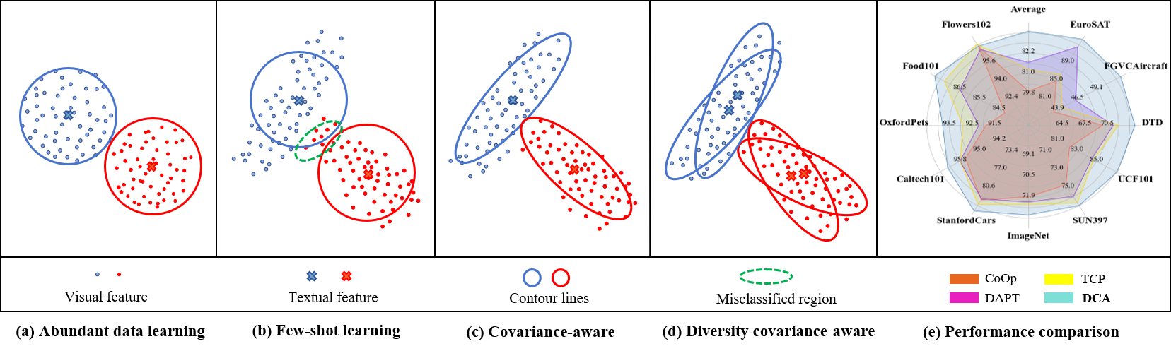
Figure 1: Illustration of feature space distribution and performance comparison. (a) When training data is abundant, DNN learns a good isotropic spherical feature space [14], and thus, isotropic metrics (such as cosine or Euclidean distance) can be effectively applied. (b) However, in few-shot tasks, isotropic feature space becomes challenging [24, 13], and isotropic metrics can lead to misclassified regions (as shown in the green area). (c) We propose the CA method, which extracts the distribution information of the data through covariance modeling and uses anisotropic Mahalanobis distance to measure the distance. (d) The DA method is designed to combat overfitting and capture different attributes of categories, maintaining more diverse decision boundaries. (e) The DCA method surpasses state-of-the-art methods on 11 diverse datasets.

The mainstream approaches for improving the transfer ability of VLMs apply the prompting technique. Earlier methods [30, 31] rely on manually crafting templates based on prior human knowledge (e.g., “a photo of a [label]”). However, designing suitable manual prompts requires domain expertise and is a labor-intensive engineering technique. Thus, recent approaches have proposed soft prompts for prompt tuning, which involves optimizing learnable vectors in either the text or visual modality. Out of these, CoOp [49] and VPT [19] fine-tune CLIP by optimizing a continuous set of prompt vectors within its language branch or image branch, respectively. Since tuning prompts in only one branch of CLIP limits the flexibility to adjust visual and textual representation spaces in downstream tasks [22], subsequent approaches [22, 5, 45, 9] began to optimize both branches. For example, MaPLe [22] proposes multi-modal prompts for both vision and language branches to enhance alignment. DAPT [5] optimizes both modalities’ prompts through metric learning to adjust the arrangement of the latent space.

Despite their decent performance, existing methods  [22, 5, 45, 9] have a significant drawback due to the nature of few-shot learning, namely, neglecting the impact of the feature space distribution. When deep neural networks learn from limited data, they are unable to obtain the uniform and isotropic spherical representation [14] that can be achieved with abundant data, which feature distribution tends to be heterogeneous [24] (as shown in Fig. 1 (a) and (b)). Consequently, during the testing phase, existing methods that rely on isotropic distances (such as cosine or Euclidean distance) to measure the distance between text and image features are suboptimal. From Fig. 1 (b), we can observe the misclassification region within the green curve. This occurs because the impact of the true feature space distribution is overlooked, which weakens the discriminative ability between features of different categories.

In this paper, we propose the diversity covariance-aware (DCA) framework as a way to learn distribution information from the data, which can effectively adapt the pre-trained VLM to downstream few-shot tasks. First, covariance-aware (CA), we demonstrate that a Bayesian classifier [24, 13] can be used by modeling the covariance relationships among visual features and utilizing text features as the average vector of these visual features. Specifically, we calculate the covariance matrix for each class from the corresponding visual feature of the training samples and replace the suboptimal cosine distance with the anisotropic Mahalanobis distance when measuring the distance between the two modalities. By considering covariance when calculating distances, the prompt model can better capture more complex class structures in high-dimensional feature spaces, thereby enhancing discrimination between features of different classes, as illustrated in Fig 1 (c). Furthermore, we enhance the commonly used loss function [44, 5] by integrating covariance modeling, thereby improving the ability to adjust intra-class relationships. Second, diversity-aware (DA), we learn multiple distinct and informative soft prompts within the text encoder to capture the diverse attributes of categories and align them with the distribution of the visual modality. Concretely, we extend multiple text prompts of varying lengths and model them independently as mean vectors in the covariance modeling. This multi-center covariance modeling effectively alleviates overfitting to limited samples, thereby better simulating the true feature space distribution (See in Fig. 1 (d)). Also, we introduce the text separation loss to ensure that different text prompts for the same class capture more comprehensive information.

To verify the effectiveness of our method, we perform experiments across different datasets, focusing on various tasks and we achieve significant performance improvements over the SOTA approaches, shown in Fig. 1 (e). The main contributions of this paper are summarized as follows:

• We propose the diversity covariance-aware (DCA) framework, which learns distributional information from the data to enhance the few-shot ability of the prompt model.

• We suggest the covariance-aware (CA) method that uses anisotropic Mahalanobis distance instead of cosine distance to measure two modalities by modeling the covariance relationships between visual features.

• We propose a diversity-aware (DA) method that learns multiple independent soft prompts within the text encoder to achieve multi-centered covariance modeling, leading to more diverse decision boundaries.

• Extensive comparative results and ablation studies across various datasets demonstrate the effectiveness of the proposed DCA framework.

2 Relate work

Vision-Language Models. Recently, using extensive image-text data in pre-trained vision-language models (VLMs) to explore the semantic correspondence between vision and language has become a trend [32, 18, 41]. Among these, CLIP [32] aggregates 400 million image-text pairs and employs a contrastive objective to learn vision-language representations. ALIGN [18] leverages a dataset of 1.8 billion noisy image-text pairs. Then, several approaches [40, 12] have emerged that enhance the capabilities of VLM by refining the latent space. These VLMs demonstrate impressive performance across various downstream tasks [49, 10, 38, 11, 4]. Currently, the mainstream solutions for visual cognition tasks are prompt tuning [49, 5] and adapter tuning [46, 10, 47, 35, 25]. This paper focuses on the former, i.e. prompt learning, aiming for fewer parameters and greater efficiency.

Prompt Learning. Prompt learning reformulates downstream tasks as pre-training tasks using prompts, effectively adapting pre-trained knowledge by minimizing domain shifts. Early approaches [30, 31] relied on manually crafting templates based on prior human knowledge. Additionally, methods using mining techniques and gradient-based approaches [20, 34] have been developed to discover suitable prompt templates automatically. In addition to hard prompt methods, computer vision has actively explored soft prompts, which involve optimizing learnable vectors in either the text or visual modality. Out of those, CoOp [49] fine-tunes CLIP by optimizing a continuous set of prompt vectors within its language branch. CoCoOp [48] learns a lightweight network to generate input condition vectors for each image. Other approaches, such as ProDA [26], PLOT [3], and KAPT [21] employ multiple text prompts or introduce external information, such as Wikipedia or GPT-3 [2], to enrich the descriptions of text prompts. Recently, some methods have proposed real-time adjustments to the visual modality. For instance, VPT [19] enhances visual ViT with learnable vectors for prompt tuning. MaPLe [22] introduces a multi-modal prompt learning approach by jointly learning hierarchical prompts in both. DAPT [5] adjusts the arrangement of the latent space to align the two modalities by multiple loss functions. LAMM [9] proposes a hierarchical loss that addresses the discrepancy in class label representations between VLMs and downstream tasks. Also, TCP [45] proposes text-based class-aware prompt tuning, explicitly incorporating prior knowledge about classes to enhance their discriminability.

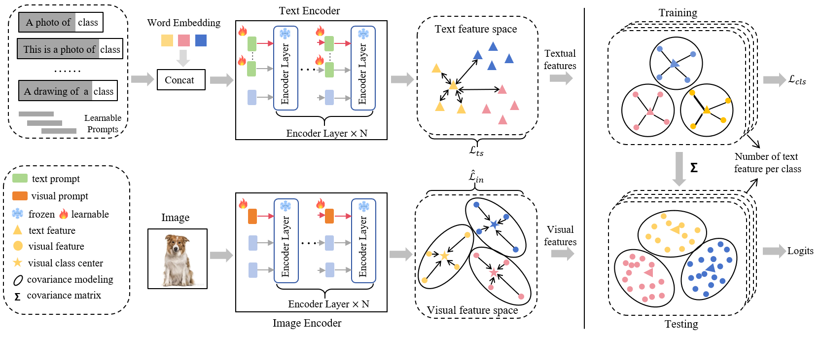
Figure 2: Overview of the architecture of DCA. DCA first uses multiple prompts to describe each class, generating multiple sets of text features through a text encoder. The images are also encoded into a set of visual features. During training, we independently compute the $\mathcal{L}_{cls}$ between multiple sets of text features and visual features. Meanwhile, we model the covariance relationships between visual features and treat the text features as their average vector, enabling the use of Mahalanobis distance to measure the similarity between text and visual feature modalities during testing. Moreover, we introduce $\mathcal{L}_{ts}$ and improve $\hat{\mathcal{L}}_{in}$ to optimize text and visual feature spaces. The detailed training and testing algorithms are provided in the appendix.

3 Method

3.1 Preliminary: Prompting for Baseline

The CLIP [32] model is a typical dual-encoder architecture consisting of an image encoder $z(\cdot)$ and text encoder $g(\cdot)$, which transforms image and text labels into visual and text features, respectively. The training objective is to align the image-text feature pair with contrastive learning on a large-scale dataset.

Text modality. Soft prompt tuning has been widely applied in the CLIP text encoder. Specifically, the text prompt $p$ consists of learnable vectors $\mathbf{w}=\{w_{l}\mid l=1,\ldots,L\}$ combined with class name. Each vector has the same dimension as the original word embedding, and $L$ represents the length of the context words. The text prompt can be formulated as $p=[w_{1},w_{2},\cdots,w_{L},\text{class}]$, where class is the word embedding of the class. With $p$ as the input, the text encoder $g(\cdot)$ outputs the text feature as $\mu=g(p)$.

Visual modality. In visual cognition, some methods propose applying soft prompt tuning in the visual encoder, specifically using visual prompt vectors $\mathbf{v}=\{v_{l}\mid l=1,\ldots,L\}$. These vectors are typically embedded between the class token CLS and the image tokens $E$. Similar, the visual prompt can be formulate as $q=[\text{CLS},v_{1},v_{2},\cdots,v_{L},E]$. With $q$ as the input, the image encoder $z(\cdot)$ outputs the visual feature as $f=z(q)$.

Prompt Tuning. Given the normalized image-text feature pair $(f,u)$, the prediction probability is calculated by using softmax with the cosine similarity between the image feature and the corresponding text feature of the image categories as follows:

$$p(c=y\mid x)=\frac{\exp(\cos(f,u_{y})/\tau)}{\sum_{j=1}^{N}\exp(\cos(f,u_{j})/\tau)},$$ (1)

where $\cos(f,\mu_{y})$ denotes the cosine distance, $\tau$ is the temperature, $N$ is the total number of image classes and $\mu_{y}$ represents the text feature of the class label $y$. Then, we can optimize the weight of $\mathbf{w}$ and $\mathbf{v}$ with cross-entropy loss between the prediction probability and the labeled target.

3.2 Covariance-Aware Prompt Learning.

Modeling Features with Covariance Relations. Considering the feature distribution heterogeneity due to data scarcity, we adopt an anisotropic Gaussian distribution $\mathcal{N}(\mu_{y},\Sigma_{y})$ to model the feature distribution of class $y$ under the few-shot setting. The probability of a feature $x$ belonging to class $y$ can be expressed as follows:

$$P(x\mid c=y)=k\exp\left(-\frac{1}{2}(x-\mu_{y})^{T}\Sigma^{-1}_{y}(x-\mu_{y})\right)$$ (2)

where $k=\frac{1}{\sqrt{(2\pi)^{D}|\Sigma_{y}|}}$ is a constant and $\mu_{y}=\frac{1}{N_{i}}\sum_{n=1}^{N_{i}}x_{i}$ is the average feature vector of all feature of class $y$. $x,\mu_{y}\in R^{D}$ and $\Sigma^{-1}_{y}$ is an arbitrary positive definite matrix. Based on the principle of maximization and Bayes’ theorem, we can arrive at the following optimal Bayesian classifier:

$$\arg\max_{y}P(Y\mid X)=\arg\max_{y}\log P(X\mid Y),$$ (3)

where the detailed intermediate derivation process is provided in the appendix. Subsequently, by substituting Eq. 2 into the right side of Eq. 14 and eliminating the irrelevant constant $k$, we obtain the following formulation:

$$\arg\max_{y}P(Y\mid X)=\arg\min_{y}\,(x-\mu_{y})^{T}\Sigma^{-1}_{y}(x-\mu_{y}),$$ (4)

where $(x-\mu_{y})^{T}\Sigma_{y}^{-1}(x-\mu_{y})$ is precisely the squared Mahalanobis distance. For convenience, $(x-\mu_{y})^{T}\Sigma_{y}^{-1}(x-\mu_{y})$ can be denoted as $d_{m}(x,\mu_{y})$. Based on the above derivation, we convert the Bayesian classification problem into the problem of minimizing the Mahalanobis distance between features and class means. Therefore, we can solve the probability problem using the Mahalanobis distance

Covariance Modeling in Visual-Language Models. Extensive literature researches indicate that the key to prompt tuning is achieving feature space alignment between the two modalities through learnable vectors, specifically the alignment between visual features $f$ and text features $\mu$. In the few-shot learning task, multiple visual features $f$ gradually align with a single text feature $\mu$ during training, and the category of a visual feature $f$ is determined by its distance to different text features $\mu$ during testing. Therefore, we can treat the text feature $\mu$ as the average vector of visual features from the same class to establish covariance relationships.

Specifically, for any pair of visual-text features $(f,\mu_{y})$, we can calculate the Mahalanobis distance between them as:

$$d_{m}(f,u_{y})=(f-\mu_{y})^{T}\mathbf{\Sigma}_{y}^{-1}(f-\mu_{y}).$$ (5)

However, in a few-shot setting, the number of samples for a class is much smaller than the feature dimension, making the covariance matrix $\Sigma$ non-invertible and impossible to compute. Therefore, we perform the covariance shrinkage [24, 13] to obtain a full-rank matrix as follow:

$$\Sigma_{s}=\Sigma+\gamma_{1}V_{m}I+\gamma_{2}V_{n}(1-I),$$ (6)

where $V_{n}$ is the average diagonal variance and $V_{m}$ is the average off-diagonal covariance of $\Sigma$. Then, to prevent excessive differences in covariance matrices across different classes, we normalize each class full-rank covariance matrix $\Sigma_{s}$ to obtain $\hat{\Sigma}_{s}$. Thus, Eq 5 can be improved as:

$$\hat{d}_{m}(f,u_{y})=(f-\mu_{y})^{T}\mathbf{(\hat{\Sigma}}_{y})_{s}^{-1}(f-\mu_{y}).$$ (7)

According to Eq.4, we treat maximizing the probability as a problem of minimizing the Mahalanobis distance. Therefore, combining Eq.1, 4, and 7, the prediction probability formula for the VLMs after covariance modeling in the visual and text feature spaces is as follows:

$$p(c=y\mid x)=\frac{\exp(\tau/(\hat{d}_{m}(f,u_{y})+\varepsilon))}{\sum_{j=1}^{N}\exp(\tau/(\hat{d}_{m}(f,u_{j})+\varepsilon))},$$ (8)

where $\varepsilon$ is a small positive number for numerical stability. Then we optimize the model for image classification on the downstream data $D$ with cross-entropy loss, ${\mathcal{L}}_{cls}$, as:

$${{\mathcal{L}}_{cls}}=-\tfrac{1}{{N_{D}}}\sum\limits_{i=1}^{{{{N}}_{D}}}{({y_{i}}\cdot\log({p_{i}})}),$$ (9)

where ${{{N}}_{D}}$ is the image number of dataset ${\mathcal{D}}$, $y_{i}$ and $p_{i}$ are the true label and the predicted for input image ${{\boldsymbol{x}}_{i}}$. Considering the properties of the Bayesian classifier, we use Mahalanobis distance only during the testing (only compute the final epoch per-class covariance matrices). Thus, during training, we simplify the covariance matrix in Eq. 7 to the identity matrix (i.e., use Euclidean distance $d_{e}$). Moreover, in cases with too few training samples (e.g. 1-shot), we treat all categories in the dataset as a single category to calculate a unified covariance matrix to model the feature space.

Covariance Modeling in Intra-class Loss. In classification tasks, some approaches [37, 42] use loss functions to minimize intra-class feature distances, thereby enhancing the discriminative power of deep features. Such loss functions are also applied in the VLM tasks [5, 44] as follows:

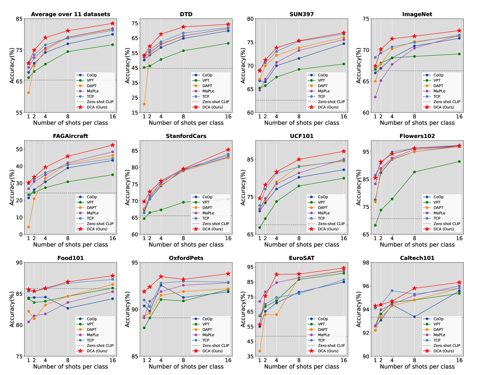
Figure 3: Comparison results (%) of few-shot learning on 11 datasets. We compared our method with several SOTA prompt learning methods and consistently demonstrated significant performance improvements across most datasets. More detailed comparison results and variance of the DCA method are provided in the appendix.

$$\mathcal{L}_{in}=\sum_{i}\left\|f_{i}-c_{y_{i}}\right\|_{2}^{2},$$ (10)

where $f_{i}$ is the visual feature, $c_{y_{i}}$ is the center of features. Based on the assumption of anisotropic Gaussian distributions in the feature space for few-shot tasks, we model the covariance in the intra-class loss $\mathcal{L}_{in}$ as follows:

$${\hat{\mathcal{L}}}_{in}=\sum_{i}(f_{i}-c_{y_{i}})^{T}\mathbf{(\hat{\Sigma}}_{y_{i}})_{s}^{-1}(f_{i}-c_{y_{i}}),$$ (11)

where $\mathbf{(\hat{\Sigma}}_{y_{i}})_{s}^{-1}$ is the covariance matrix of class $y_{i}$. During training, we compute the covariance matrix only at the first epoch, which significantly reduces the computational burden and effectively maintains the generalization ability of the original CLIP, preventing overfitting.

3.3 Diversity-Aware Prompt Learning

Even though soft prompts are highly robust, learning a single sentence is insufficient to represent a class. Thus, we learn multiple distinct soft prompts in the text encoder to capture different attributes of a category and its visual representation distribution.

Specifically, compared to the baseline, we extend to multiple learnable vectors $\mathbf{w}^{1},\ldots,\mathbf{w}^{M}$ for each class and create $M$ text prompts $p^{1},\ldots,p^{M}$. Given an input image $x$, we obtain the normalized image feature $f$. We then input $M$ text prompts into the text encoder to get $M$ text features $u^{1},\ldots,u^{M}$, resulting in $M$ pairs of text features $(f,u^{m})$. We then calculate the prediction probabilities for each pair using Eq. 8, compute the cross-entropy loss for each pair using Eq. 9, and sum these losses to obtain the final loss. Notably, during training, we compute the loss function independently for different text prompts of the same class. This encourages the text prompts to capture various aspects of the visual features, leading to a more comprehensive representation of the class. During testing, we compute the prediction probabilities for the $M$ text-image pairs using Eq. 8 and average these probabilities to determine the final result.

Moreover, we introduce a text separation loss $\mathcal{L}_{ts}$ to ensure that text prompts for the same class capture more comprehensive information and to address issues with visual feature alignment caused by small distances between text features of different classes. Specifically, we obtain $M\times C$ text features during training, where $C$ is the total number of classes. We define these features as the set $A$. For each pair of $u_{i}$ and $u_{j}$ randomly selected from the instance set $A$, The text separation loss can be formulated as:

$$\mathcal{L}_{ts}=-\sum_{i\neq j}||u_{i},u_{j}||^{2}_{2}.$$ (12)

3.4 Object Optimization.

We optimize the weights of the prompts $\mathbf{w}$ and $\mathbf{v}$ using three loss functions: (1) the classification loss ${\mathcal{L}}_{cls}$ in Eq. 9, (2) the Mahalanobis intra-class loss $\hat{\mathcal{L}}_{in}$ in Eq. 11, and (3) the text separation loss $\mathcal{L}_{ts}$ in Eq. 12. The total loss function is then obtained as follows:

$${\mathcal{L}}={{\mathcal{L}}_{cls}}+\alpha{\hat{{\mathcal{L}}}_{in}}+\beta{{\mathcal{L}}_{ts}},$$ (13)

where $\alpha$ and $\beta$ are hyper-parameters.

4 Experiment

4.1 Experimental Setup

Dataset and Protocols. We followed the settings of previous works [49, 19] for both the few-shot learning and domain generalization. In the few-shot setting, we evaluate 11 public datasets including DTD [6], FGVCAircraft [27], Food101 [1], ImageNet [7], StanfordCars [23], Caltech101 [8], Flowers102 [28], OxfordPets [29], SUN397 [43], UCF101 [36], and EuroSAT [15]. All experiments adopted protocol in CLIP [32], which learns with 1, 2, 4, 8, and 16 labeled samples per class. For the domain generalization setting, we use ImageNet as the source domain and test robustness on target datasets, including ImageNet-A [17], ImageNet-R [16], ImageNet-Sketch [39], and ImageNet-V2 [33].

Table 1: Comparison to state-of-the-art methods for few-shot learning of CLIP-based models, using ViT-B/16 backbone. * indicates the reproduced results where we replace their backbone with VIT-B/16. The best results are in bold.

Method	K=1	K=2	K=4	K=8	K=16
Adapter-tuning methods
$\text{TIP-Adapter}_{\text{ ECCV22}}$ [46]	69.81	71.56	74.18	75.17	77.39
$\text{TIP-Adapter-F}_{\text{ ECCV22}}$ [46]	70.86	73.10	76.04	78.81	81.27
$\text{Cross-Modal}_{\text{ CVPR23}}$ [25]	70.75	73.29	76.79	79.05	80.75
$\text{CLAP*}_{\text{ CVPR24}}$ [35]	70.71	73.81	77.59	80.02	81.92
Prompt-tuning methods
$\text{CoOP}_{\text{ IJCV22}}$ [49]	67.82	70.73	74.19	76.95	80.02
$\text{VPT}_{\text{EECV22}}$ [19]	66.16	68.12	70.46	74.47	76.68
$\text{CoCoOP}_{\text{ CVPR22}}$ [48]	66.79	67.65	72.21	72.96	74.92
$\text{DAPT}_{\text{ ICCV23}}$ [5]	61.32	69.92	75.02	79.03	81.66
$\text{MaPLe}_{\text{ CVPR23}}$ [22]	69.40	72.51	75.62	79.13	81.87
$\text{LAMM}_{\text{ AAAI24}}$ [22]	68.99	73.09	75.95	78.54	81.13
$\text{TCP}_{\text{ CVPR24}}$ [45]	70.85	73.46	76.62	78.73	81.27
DCA	70.92	74.93	78.95	81.16	83.51

Table 2: Comparison results of domain generalization.

Method	ImageNet	-V2	-Sketch	-A	-R
CLIP [32]	66.72	60.90	46.10	47.75	73.97
CoOp [49]	71.93	64.22	47.07	48.97	74.32
VPT [19]	69.31	62.36	47.72	46.20	75.81
MaPLe [22]	70.72	64.07	49.15	50.90	76.98
DAPT [5]	72.20	64.93	48.30	48.74	75.75
TCP [45]	71.20	64.60	49.50	51.20	76.73
DCA (Ours)	72.92	66.22	49.53	47.86	76.53

Compare Methods. We compare several classical prompt learning methods, including CoOP [49] and VPT [19]. We also compare our approach with SOTA methods such as MaPLe [22], DAPT [5], and TCP [45]. Moreover, we compare with several SOTA adapter-tuning methods, including Tip-Adapter [46], Cross-Modal [25], and CLAP [35].

Implementation Details. Our implementation is based on the ViT-B/16 variant of the CLIP model. We set the length of the visual prompt to 16 and configured the text prompt lengths to range from 3 to 6. The number of text prompts $M$ is set to 4. We evaluate all experiments with three seeds and report the average value. More details are provided in the appendix.

Table 3: Ablation study of proposed DCA. We adopt CA, ${\hat{{\mathcal{L}}}_{in}}$, DA and ${\mathcal{L}}_{ts}$ to denote covariance-aware, Mahalanobis intra-class loss diversity-aware and text separation loss.

CA	${\hat{{\mathcal{L}}}_{in}}$	DA	${\mathcal{L}}_{ts}$	DTD	FGVCAircraft	StanfordCars	Flowers102	UCF101	Food101	EuroSAT
				60.91	29.89	72.01	90.95	79.12	83.12	84.33
✓				63.81	31.11	72.93	91.85	79.81	84.13	87.53
✓	✓			64.39	33.94	73.84	91.95	80.62	84.72	88.72
✓		✓		64.94	36.65	74.45	93.88	80.92	84.55	88.92
✓	✓	✓		65.54	38.78	74.98	93.96	81.15	84.74	88.95
✓	✓	✓	✓	67.61	39.39	75.96	94.29	81.66	85.12	89.98

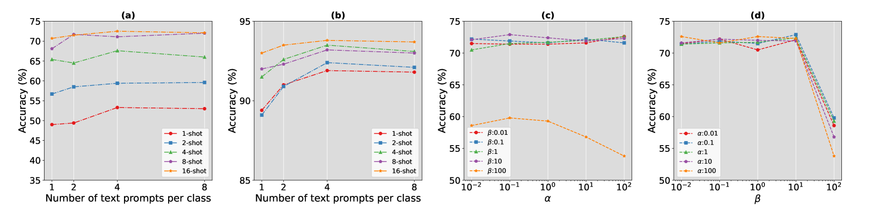
Figure 4: (a,b) The influence of text prompt number $M$. (c,d) Sensitivity analysis of hyper-parameters.

4.2 Few-shot Learning

We present the comparative results with SOTA methods in Fig. 3 and Table 1. We summarize the result as follows:

• For most datasets, all tuning methods outperform zero-shot CLIP. Our DCA demonstrates a more significant performance improvement, achieving a maximum boost of 18.16% at 16 shots.

• For the adapter-tuning methods, our approach achieves a performance improvement with fewer additional parameters and higher efficiency, with a maximum improvement of 1.59% at 16 shots.

• Compared to classical methods such as CoCo and VPT, the DCA consistently improves all shots. For instance, DCA provides an average absolute gain ranging from 4.76% to 8.46% from 1 to 16 shots. For CoOp, we also achieved an average improvement of 3.95%, with a maximum improvement of 4.76% at 4 shots.

• For the SOTA methods, such as MaPLe, DAPT, and TCP, our DCA also achieves significant improvements, especially with increases of at least 2.33%, 2.06%, and 1.64% from 4 to 16 shots, respectively. Notably, our method maintains stable performance across different shots, avoiding the severe performance drop observed with the DAPT at 1 shot, demonstrating its robustness.

4.3 Domain Generalization

We evaluate the generalization of DCA by comparing it with zero-shot CLIP and prompt learning methods in a domain-generalization setting. We use ImageNet as the source dataset, with prompts trained on 16 samples, and four datasets as the target datasets. The overall results are shown in Table 2 and we can summarize that:

• DCA achieves significant performance improvements on unseen data compared to zero-shot CLIP, with a maximum increase of 5.32% on ImageNet-V2.

• For DAPT, which also focuses on few-shot tasks like ours, our method demonstrates superior performance across most datasets with a significant accuracy gain, showcasing better generalization.

• For methods that focus more on generalization, such as MaPLe and TCP, accuracy decreases on ImageNet-A and ImageNet-R, respectively. In contrast, on the remaining datasets, especially ImageNet-V2, there is up to a 1.62% improvement.

4.4 Ablation Study

Table 4: The effectiveness analysis of covariance modeling in visual-language models.

Method	FGVCAircraft					DTD					Caltech101
	1	2	4	8	16	1	2	4	8	16	1	2	4	8	16
Baseline+$d_{cos}$	10.28	15.22	29.96	40.82	46.27	9.28	45.32	60.93	65.09	70.52	91.78	92.68	92.69	94.78	95.75
Baseline+$\boldsymbol{d_{m}}$	16.62	20.88	31.11	41.72	46.98	10.98	57.18	63.81	69.46	70.73	92.32	93.84	94.16	95.21	95.84
DAPT+$d_{cos}$	4.32	20.90	32.88	41.39	46.29	20.61	54.55	60.68	66.38	71.28	92.18	93.28	94.29	94.77	95.76
DAPT+$\boldsymbol{d_{m}}$	16.33	21.64	33.94	42.62	49.08	21.88	57.22	62.41	69.63	71.58	92.94	93.84	94.43	95.21	96.18
DCA+$d_{cos}$	26.11	31.62	36.92	44.35	51.12	47.93	53.45	63.12	68.32	72.14	89.92	92.31	92.87	94.46	95.38
DCA+$\boldsymbol{d_{m}}$	30.33	33.64	39.39	45.82	52.38	53.32	59.42	67.61	72.52	74.25	94.34	94.42	94.71	95.81	96.34

The Effectiveness of Each Component. To demonstrate how each component of the proposed DCA contributes to performance improvements, we conducted ablation studies of 4-shot learning on 7 datasets. Table  3 shows the results and we can observe that:

• All components in DCA consistently improve the baseline performance without any conflicts between them. The improvements are particularly notable on challenging datasets, e.g. DTD and FGVCircraft, where the cumulative improvements are 6.70% and 9.50%, respectively.

• Compared to the baseline, the CA method significantly improves across multiple datasets, with a maximum gain of 3.20% on EuroSAT. This validates our hypothesis that feature spaces in few-shot learning tasks benefit more from anisotropic distances, i.e. Mahalanobis distance. The DA method consistently enhances CA’s performance across all datasets, achieving up to 5.54% improvement on FGVCAicraft, showing that multi-centered covariance modeling enhances decision boundaries.

• The Mahalanobis intra-class and text separation losses respectively increase performance by an average of 1.0% and 0.95%, demonstrating that these loss functions can further optimize the feature space, enhancing the effectiveness of both CA and DA methods.

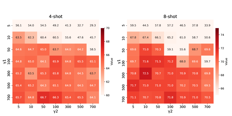
Figure 5: Impact of covariance shrinkage parameter $\gamma_{1}$ and $\gamma_{2}$.

The Ablation Study of Text Prompt Number. As discussed in Sec. 3.3, $M$ represents the number of text prompts. We conduct an ablation study to evaluate the impact of the number of text prompts per class. Fig. 4 (a) and (b) show the results on the DTD and OxfordPet. We observed that two datasets showed consistent results: (1) performance increases as the number of text prompts increases, indicating that more text prompts can help learn comprehensive visual information. (2) Notably, performance peaks at $M$=$4$ and begins to decline slightly as $M$ increases, suggesting that too many prompts can lead to information redundancy, which is detrimental to optimization.

The Sensitivity of Hyper-parameter. (1) The hyper-parameters $\alpha$ and $\beta$ adjust the strength of the Mahalanobis intra-class loss and the text diversity loss. We conducted a sensitivity study on the DTD dataset, where we varied the values of $\alpha$ and $\beta$ within the reasonable range of $\{10^{-2},10^{-1},1,10^{1},10^{2}\}$, respectively. As shown in Fig. 4 (c) and (d), except for $\beta$ being $10^{2}$, the performance of DCA varies only slightly and shows consistent performance across a wide range of hyper-parameters. These indicate the robustness of our method.

(2) We also analyzed the effects of the covariance shrinkage parameters $\gamma_{1}$ and $\gamma_{2}$ in the few-shot settings. Take DTD as an example, as shown in Fig. 5. Our observations indicate that the model performance remained stable for both the 4-shot and 8-shot settings and achieved optimal results when $\gamma_{1}\in[100,700]$ and $\gamma_{2}\in[5,500]$. Similarly, we can obtain the optimal values of $\gamma_{1}$ and $\gamma_{2}$ for the other 10 datasets under different shot settings.

Due to the different characteristics of each dataset and each shot setting, there may be different optimal parameter values. Therefore, we provide the optimal hyper-parameters for each dataset and each shot setting in the appendix.

4.5 Analysis

The Effectiveness of Covariance Modeling in VLMs. Compared to other methods using cosine distance, we use Mahalanobis distance to measure the distance of text and image features. To further verify the effectiveness of the CA method, we applied it to the baseline and SOTA method DAPT across three datasets. Table 4 shows the experimental results for 1$\sim$16 shots. We can observe that covariance modeling consistently improves performance across the three datasets, especially when the training samples are limited, such as in the 1-shot setting. For example, it improves the baseline and DAPT by 6.34% and 12.01%, respectively, on FGVCAircraft. In addition, compared with cosine distance, using Mahalanobis distance also has a significant effect on our method.

Table 5: The effectiveness analysis of covariance modeling in intra-class loss.

Method	Average over 11 datasets
	4 shots	16 shots
$\mathcal{L}_{in}$-L1	77.96 ($\downarrow$ 0.99)	82.62 ($\downarrow$ 0.89)
$\mathcal{L}_{in}$-L2	78.02 ($\downarrow$ 0.81)	82.70 ($\downarrow$ 0.72)
$\mathcal{L}_{in}$-$d_{m}$ (ours)	78.95	83.51

The Effectiveness of Mahalanobis Intra-class Loss. We use Mahalanobis distance instead of Euclidean distance to achieve intra-class contraction. To demonstrate the performance improvement of the loss function with Mahalanobis distance, we conducted analytical experiments on 11 datasets. As shown in Table 4, using Mahalanobis distance results in performance improvements for both 4-shot and 16-shot settings, with maximum increases of 0.99% and 0.81% over L1 and L2 distance, respectively. This demonstrates that covariance modeling can adjust the loss function based on the dataset’s distribution, helping to prevent overfitting.

5 Conclusion and Limitations

We proposed a prompt learning framework called DCA for VLMs. By modeling the covariance in the visual feature space, using Mahalanobis distance to measure between text and visual modalities, and learning multiple diverse and information-rich soft prompts, our method significantly enhances prompt model performance without substantially increasing computational overhead. Meanwhile, we theoretically prove the rationality of our method. Although the proposed method significantly improves performance on few-shot tasks, it still faces challenges in model generalization tasks, such as domain generalization. Therefore, maintaining model generalization to unseen tasks during downstream training is a promising direction for future research.

6 APPENDIX

6.1 The Proof of Bayesian Classifier

In the main paper, based on the principle of maximization and Bayes’ theorem [13, 24], we obtained the following equation:

$$\arg\max_{y}P(Y\mid X)=\arg\max_{y}\log P(X\mid Y).$$ (14)

Next, we can present a detailed proof of this equation. Specifically, applying Bayes’ theorem, we have:

$$P(Y\mid X)=\frac{P(X\mid Y)P(Y)}{P(X)},$$ (15)

where $P(Y\mid X)$ represents the posterior probability of class $Y$ given $X$, $P(X\mid Y)$ denotes the likelihood of $X$ given class $Y$, $P(Y)$ refers to the prior probability of class $Y$, and $P(X)$ corresponds to the marginal probability of $X$. Since the marginal probability $P(X)$ remains constant for all $y$, it can be disregarded when maximizing $P(Y\mid X)$:

$$\arg\max_{y}P(Y\mid X) =\arg\max_{y}\frac{P(X\mid Y)P(Y)}{P(X)}$$ (16)

$$=\arg\max_{y}P(X\mid Y)P(Y).$$

Assuming the prior probabilities $P(Y)$ are identical across all classes, we take the logarithm of the expression:

$$\arg\max_{y} \log\left(P(X\mid Y)P(Y)\right)$$ (17)

$$=\arg\max_{y}\left(\log P(X\mid Y)+\log P(Y)\right)$$

$$=\arg\max_{y}\log P(X\mid Y),$$

where based on Eq. (3) and Eq. (4), we can derive Eq. (1), thus concluding the proof.

Given the anisotropic Gaussian distribution assumption $\mathcal{N}(\mu_{y},\Sigma_{y})$ to model the feature distribution of class $y$, and , we have:

$$P(x\mid c=y)=$$ (18)

$$\frac{1}{(2\pi)^{D/2}|\Sigma_{y}|^{1/2}}\exp\left(-\frac{1}{2}(x-\mu_{y})^{T}\Sigma_{y}^{-1}(x-\mu_{y})\right),$$

where $D$ is the dimensional of $x$, $\mu_{y}=\frac{1}{N_{i}}\sum_{n=1}^{N_{i}}x_{i}$ is the average feature vector of all feature of class $y$. $x,\mu_{y}\in R^{D}$ and $\Sigma^{-1}_{y}$ is an arbitrary positive definite matrix. Then, we substitute Eq. (5) into Eq. (1) to obtain the following formula:

$$\arg\max_{y}P(Y\mid X)=\arg\max_{y}\log P(X\mid Y)$$ (19)

$$=\arg\max_{y}-\frac{1}{2}\left[(x-\mu_{y})^{T}\Sigma_{y}^{-1}(x-\mu_{y})+\log|\Sigma_{y}|+D\log(2\pi)\right]$$

$$=\arg\min_{y}\,(x-\mu_{y})^{T}\Sigma^{-1}_{y}(x-\mu_{y}).$$

Therefore, based on the above derivation, we transform the Bayesian classification problem into a problem of minimizing the Mahalanobis distance.

6.2 Implementation Details

Model and Configuration. Our implementation is based on the ViT-B/16 variant of the CLIP model. We set the length of the visual prompt to 16 and configured the text prompt lengths to range from 3 to 6. The number of each class text prompts $M$ is set to 4. The text prompts are initialized with the following phrases: “A photo of [CLASS]”, “A drawing of a [CLASS]”, “This is a photo of [CLASS]”, and “This is a photo of a [CLASS]”.

Covariance Matrix Shrinkage. For stability in covariance matrix estimation, we apply shrinkage with parameters $\gamma_{1}$ and $\gamma_{2}$ for different shot settings in Table 6. This ensures that the covariance matrix remains robust throughout the training process.

Training Protocol. Following the comparative approaches (e.g. CoOp and DAPT), we train our model with different numbers of epochs depending on the few-shot setting. Specifically, we use 80 epochs for the 1-shot setting, 100 epochs for the 2-shot and 4-shot settings, and 200 epochs for the 8-shot and 16-shot settings.

Optimizer and Learning Rate Schedule. We employ the SGD optimizer for training, with the learning rate adjusted according to a cosine schedule. For warmup, we apply 5 epochs with a constant learning rate of 1e-5.

Batch Size. Similar to other approaches [5, 49], the batch size varies according to the dataset size. For smaller datasets such as FGVCAircraft, OxfordFlowers, and StanfordCars, the batch size is set to 32. For larger datasets like Imagenet and SUN397, the batch size is set to 64.

Hardware and Platform. We implemented our method with the PyTorch platform and trained on 2 RTX 3090 24G GPUs.

Seed and Averaging. To ensure the reliability of our results, all experiments are conducted with three different seeds(1/2/3), and the results are averaged across these runs, which is shown in Figure 6.

6.3 More Compare Results

In this section, we provide additional comparative methods and detailed comparative results for each experimental setup in Table 7.

6.4 Training and Testing Loop

We provide a detailed training and testing loop to help understand our DCA method in Algorithm1.

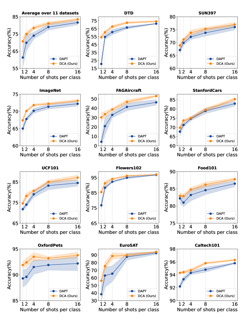
Figure 6: Robustness Analysis. Our method (DCA) is compared with the SOTA method (DAPT [5]) across eleven datasets with different random seeds. The results show that DCA achieves better average performance and exhibits lower variance, indicating superior stability and robustness under different random seed settings.

Algorithm 1 The training and testing loop of the proposed DCA method for vision-language models

1:Pre-trained visual encoder $z(\cdot)$, text encoder $g(\cdot)$, training dataset $D$, number of classes $N$, number of text prompts per class $M$, hyper-parameters $\alpha,\beta$, learning rate $\eta$

2:Optimized text prompts $\mathbf{w}$ and visual prompt $\mathbf{v}$

3:Initialization: Initialize prompts $\{\mathbf{w}^{1},\ldots,\mathbf{w}^{M}\}$ for each class, visual prompt $\mathbf{v}$, and covariance matrix $\Sigma_{y}=\mathbf{I}$ for each class $y$.

4:for each class $y$ in $N$ do

5:  Compute class center $\mu_{y}=\frac{1}{|D_{y}|}\sum_{x\in D_{y}}z(x)$

6:end for

7:while not converged do

8:  for each mini-batch $B=\{(x_{i},y_{i})\}$ from $D$ do

9:   for each image $x_{i}$ with label $y_{i}$ in $B$ do

10:     Compute visual feature $f_{i}=z(x_{i})$

11:     for each $p^{m}$ in $\{p^{1},\ldots,p^{M}\}$ do

12:      Compute text feature $u^{m}=g(p^{m})$

13:      Calculate distance $d_{e}(f_{i},u^{m})$ (Eq.7)

14:      Compute prediction probability $p(c=y_{i}\mid x_{i})$ (Eq.8)

15:      Compute cross-entropy loss $\mathcal{L}_{cls}^{m}=-\log p(c=y_{i}\mid x_{i})$ (Eq.9)

16:     end for

17:     Sum losses from all $M$ prompts to obtain $\mathcal{L}_{cls}=\sum_{m=1}^{M}\mathcal{L}_{cls}^{m}$

18:   end for

19:   Compute intra-class loss $\hat{\mathcal{L}}_{in}$ with covariance $\hat{\Sigma}_{s_{y_{i}}}$ (Eq.11)

20:   Compute text separation loss $\mathcal{L}_{ts}$ (Eq.12)

21:   Total Loss: $\mathcal{L}=\mathcal{L}_{cls}+\alpha\hat{\mathcal{L}}_{in}+\beta\mathcal{L}_{ts}$ (Eq.13)

22:   SGD Update: $\mathbf{w}\leftarrow\mathbf{w}-\eta\nabla_{\mathbf{w}}\mathcal{L}$, $\mathbf{v}\leftarrow\mathbf{v}-\eta\nabla_{\mathbf{v}}\mathcal{L}$

23:  end for

24:end while

25:Testing Phase:

26:for each test image $x$ do

27:  Compute visual feature $f=z(x)$

28:  Compute covariance matrix $\Sigma_{y}$ and apply shrinkage to obtain $\Sigma_{s_{y}}$

29:  Compute Mahalanobis distance $d_{m}(f,u_{y})$ using $\hat{\Sigma}_{s_{y}}$

30:  Predict class label based on smallest Mahalanobis distance

31:end for

Table 6: The hyper-parameters $\gamma_{1}$ and $\gamma_{2}$ for different shot settings in few-shot learning.

Hyper-parameters	Shot Settings
	1-shot	2-shot	4-shot	8-shot	16-shot
$\gamma_{1}$	500	500	600	500	500
$\gamma_{2}$	300	300	100	100	500

Table 7: Per-dataset performance comparison of DCA with various methods in few-shot setting. * denotes the performance obtained by our re-implementation. The best results are in bold and the second-best results are underlined.

Dataset	Set	CLIP	LP+CLIP	CoOp (IJCV22)	VPT (ECCV22)	CoCoOp (CVPR22)	DAPT (ICCV23)	MaPLe (CVPR23)	LAMM (AAAI24)	TCP* (CVPR24)	Ours
Average	1 shot	65.35	45.83	67.82	66.16	66.79	61.32	69.4	68.97	70.85	70.92
	2 shots	65.35	57.98	70.73	68.12	67.65	69.92	72.51	73.22	73.46	74.93
	4 shots	65.35	68.01	74.19	70.46	72.21	75.02	75.62	75.89	76.62	78.95
	8 shots	65.35	74.47	76.95	74.47	72.96	79.03	79.13	78.47	78.73	81.16
	16 shots	65.35	78.79	80.02	76.68	74.92	81.66	81.87	81.07	81.27	83.51
ImageNet	1 shot	66.67	32.13	66.33	66.91	69.43	65.01	62.47	67.22	68.82	67.43
	2 shots	66.67	44.88	67.07	67.92	69.78	67.78	65.13	68.67	69.52	70.14
	4 shots	66.67	54.85	68.73	68.73	70.39	70.16	67.72	69.88	70.53	71.82
	8 shots	66.67	62.23	70.63	68.97	70.65	71.35	70.32	71.32	71.23	72.23
	16 shots	66.67	67.31	71.87	69.36	70.83	72.22	72.33	72.71	72.4	73.13
Caltech101	1 shot	93.32	79.88	92.63	92.58	93.83	92.22	92.57	93.39	94.13	94.32
	2 shots	93.32	89.01	93.07	93.62	94.82	93.3	93.97	93.90	94.42	94.43
	4 shots	93.32	92.05	94.41	94.61	94.98	94.32	94.43	94.81	95.63	94.73
	8 shots	93.32	93.41	93.37	94.82	95.04	94.81	95.21	95.79	95.32	95.84
	16 shots	93.32	95.43	95.57	95.36	95.16	95.81	96.02	96.89	95.83	96.34
StanfordCars	1 shot	65.54	35.66	67.43	64.73	67.22	67.69	66.62	67.34	66.43	69.84
	2 shots	65.54	50.28	70.51	66.52	68.37	71.28	71.63	73.11	70.74	72.72
	4 shots	65.54	63.38	74.47	67.31	69.39	74.69	75.32	77.58	75.73	75.96
	8 shots	65.54	73.67	79.31	69.62	70.44	78.92	79.47	81.29	79.12	79.58
	16 shots	65.54	80.44	83.07	70.52	71.57	82.88	83.57	85.07	84.02	85.38
Flowers102	1 shot	70.73	69.74	77.53	68.27	69.74	76.81	83.31	84.49	86.41	85.51
	2 shots	70.73	85.07	87.33	73.81	85.07	88.41	88.93	91.72	90.81	91.31
	4 shots	70.73	92.02	92.17	77.83	92.02	92.31	92.67	93.23	94.91	94.21
	8 shots	70.73	96.11	94.97	87.62	96.11	95.01	95.81	95.89	96.31	96.21
	16 shots	70.73	97.35	97.07	91.42	97.37	96.81	97.01	97.38	97.31	97.11
FGVCAircraft	1 shot	24.31	19.61	21.37	23.26	12.68	4.32	26.73	27.72	29.71	30.33
	2 shots	24.31	26.41	26.2	24.55	15.06	20.92	30.92	32.13	32.31	33.63
	4 shots	24.31	32.33	30.83	27.38	24.79	32.91	34.87	35.31	36.22	39.39
	8 shots	24.31	39.35	39.02	30.86	26.61	41.41	42.02	40.67	40.73	45.83
	16 shots	24.31	45.36	43.42	34.98	31.21	46.32	48.41	45.38	44.53	52.38
DTD	1 shot	44.61	34.59	50.23	45.19	48.54	20.61	52.13	51.69	53.41	53.31
	2 shots	44.61	40.76	53.60	46.21	52.17	54.62	55.51	60.01	57.01	59.43
	4 shots	44.61	55.71	58.73	50.66	55.04	60.74	61.03	64.99	62.53	67.62
	8 shots	44.61	63.46	64.77	56.51	58.89	66.42	66.52	66.91	68.43	72.52
	16 shots	44.61	69.96	69.87	61.47	63.04	71.35	71.33	72.19	72.03	74.25
SUN397	1 shot	62.61	41.58	66.77	65.22	68.33	67.13	64.77	66.69	69.12	68.94
	2 shots	62.61	53.72	66.53	65.72	69.03	69.92	67.1	69.31	70.63	71.23
	4 shots	62.61	63.02	69.97	67.54	70.21	72.22	70.67	71.72	73.01	73.84
	8 shots	62.61	69.08	71.53	69.19	70.84	73.83	73.23	75.56	75.22	75.32
	16 shots	62.61	73.28	74.67	70.35	72.15	76.04	75.53	76.12	76.73	77.05
Food101	1 shot	85.85	43.96	84.33	84.21	85.65	82.21	80.51	82.29	85.41	85.66
	2 shots	85.85	61.51	84.41	83.61	86.22	81.01	81.47	83.52	85.41	85.62
	4 shots	85.85	73.19	84.47	83.81	86.88	83.21	81.77	84.09	85.81	85.88
	8 shots	85.85	79.79	82.67	84.61	86.97	84.61	83.61	85.34	86.71	87.88
	16 shots	85.85	82.91	84.21	85.91	87.25	86.51	85.33	86.43	87.31	87.41
UCF101	1 shot	67.57	53.66	71.23	66.82	70.31	71.83	71.83	72.18	72.71	74.61
	2 shots	67.57	65.78	73.43	69.19	73.51	74.01	74.61	75.76	77.11	78.21
	4 shots	67.57	73.28	77.11	73.76	74.82	79.01	78.47	79.49	81.31	81.66
	8 shots	67.57	79.34	80.21	77.91	77.14	83.21	81.37	81.09	83.01	85.01
	16 shots	67.57	82.11	82.23	79.97	78.14	84.51	85.03	83.77	84.71	87.15
OxfordPets	1 shot	89.11	44.06	90.37	88.03	91.27	89.31	89.10	88.47	91.02	91.91
	2 shots	89.11	58.37	89.80	89.09	92.64	89.62	90.87	90.21	90.31	92.42
	4 shots	89.11	71.17	92.57	91.05	92.81	91.51	91.90	91.86	92.82	93.52
	8 shots	89.11	78.36	91.27	90.91	93.45	91.91	92.57	92.73	93.02	93.21
	16 shots	89.11	85.34	91.87	92.11	93.34	92.22	92.83	93.11	92.92	93.82
EuroSAT	1 shot	48.43	49.23	54.93	62.12	55.33	38.4	71.82	57.23	62.43	56.23
	2 shots	48.43	61.98	65.17	68.42	46.74	63.02	78.32	67.06	70.08	75.53
	4 shots	48.43	77.09	70.81	72.36	65.56	63.03	84.51	71.83	74.52	89.98
	8 shots	48.43	84.43	78.07	86.58	68.21	87.82	87.73	77.56	77.12	90.22
	16 shots	48.43	87.21	84.93	90.78	73.32	92.61	92.33	82.75	86.42	94.33

6.5 Parameter Table

Due to the different characteristics of each dataset, there may be different optimal parameter values. Therefore, we provide the optimal hyper-parameters for each dataset in Table 8.

Table 8: The parameters table of DCA method on 11 datasets in few-shot learning.

Hyperparameters	DTD	FGVCAircraft	SUN397	Caltech101	OxfordPets	Food101	Flowers102	UCF101	StanfordCars	ImageNet	EuroSAT
$\alpha$	5.0	5.0	100.0	10.0	1.0	1.0	10.0	5.0	10.0	10.0	100.0
$\beta$	0.5	0.01	0.01	0.01	0.1	0.5	0.5	0.1	0.5	0.1	2.0
Learning rate	20.0	2.0	20.0	0.2	0.02	20.0	0.002	20.0	0.2	2.0	20.0

References

- Bossard et al. [2014] Lukas Bossard et al. Food-101–mining discriminative components with random forests. In Computer Vision–ECCV 2014: 13th European Conference, Zurich, Switzerland, September 6-12, 2014, Proceedings, Part VI 13, pages 446–461. Springer, 2014.
- Brown et al. [2020] Tom Brown, Benjamin Mann, Nick Ryder, et al. Language models are few-shot learners. Advances in neural information processing systems, 33:1877–1901, 2020.
- Chen et al. [2022] Guangyi Chen, Weiran Yao, Xiangchen Song, Xinyue Li, Yongming Rao, and Kun Zhang. Prompt learning with optimal transport for vision-language models. 2022.
- Chen et al. [2023] Guangyi Chen, Xiao Liu, Guangrun Wang, Kun Zhang, Philip HS Torr, Xiao-Ping Zhang, and Yansong Tang. Tem-adapter: Adapting image-text pretraining for video question answer. In Proceedings of the IEEE/CVF International Conference on Computer Vision, pages 13945–13955, 2023.
- Cho et al. [2023] Eulrang Cho et al. Distribution-aware prompt tuning for vision-language models. In Proceedings of the IEEE/CVF International Conference on Computer Vision, pages 22004–22013, 2023.
- Cimpoi et al. [2014] Mircea Cimpoi, Subhransu Maji, Iasonas Kokkinos, Sammy Mohamed, and Andrea Vedaldi. Describing textures in the wild. In Proceedings of the IEEE conference on computer vision and pattern recognition, pages 3606–3613, 2014.
- Deng et al. [2009] Jia Deng, Wei Dong, Richard Socher, Li-Jia Li, Kai Li, and Li Fei-Fei. Imagenet: A large-scale hierarchical image database. In 2009 IEEE conference on computer vision and pattern recognition, pages 248–255. Ieee, 2009.
- Fei-Fei et al. [2004] Li Fei-Fei et al. Learning generative visual models from few training examples: An incremental bayesian approach tested on 101 object categories. In 2004 conference on computer vision and pattern recognition workshop, pages 178–178. IEEE, 2004.
- Gao et al. [2024a] Jingsheng Gao, Jiacheng Ruan, Suncheng Xiang, Zefang Yu, Ke Ji, Mingye Xie, Ting Liu, and Yuzhuo Fu. Lamm: Label alignment for multi-modal prompt learning. In Proceedings of the AAAI Conference on Artificial Intelligence, pages 1815–1823, 2024a.
- Gao et al. [2024b] Peng Gao, Shijie Geng, Renrui Zhang, Teli Ma, Rongyao Fang, Yongfeng Zhang, Hongsheng Li, and Yu Qiao. Clip-adapter: Better vision-language models with feature adapters. International Journal of Computer Vision, 132(2):581–595, 2024b.
- Garcia et al. [2020] Noa Garcia, Mayu Otani, Chenhui Chu, and Yuta Nakashima. Knowit vqa: Answering knowledge-based questions about videos. In Proceedings of the AAAI conference on artificial intelligence, pages 10826–10834, 2020.
- Goel et al. [2022] Shashank Goel, Hritik Bansal, Sumit Bhatia, Ryan Rossi, Vishwa Vinay, and Aditya Grover. Cyclip: Cyclic contrastive language-image pretraining. Advances in Neural Information Processing Systems, 35:6704–6719, 2022.
- Goswami et al. [2024] Dipam Goswami, Yuyang Liu, Bartłomiej Twardowski, and Joost van de Weijer. Fecam: Exploiting the heterogeneity of class distributions in exemplar-free continual learning. Advances in Neural Information Processing Systems, 36, 2024.
- Guerriero et al. [2018] Samantha Guerriero, Barbara Caputo, and Thomas Mensink. Deepncm: Deep nearest class mean classifiers. 2018.
- Helber et al. [2019] Patrick Helber, Benjamin Bischke, Andreas Dengel, and Damian Borth. Eurosat: A novel dataset and deep learning benchmark for land use and land cover classification. IEEE Journal of Selected Topics in Applied Earth Observations and Remote Sensing, 12(7):2217–2226, 2019.
- Hendrycks et al. [2021a] Dan Hendrycks, Steven Basart, Norman Mu, Saurav Kadavath, Frank Wang, Evan Dorundo, Rahul Desai, Tyler Zhu, Samyak Parajuli, Mike Guo, et al. The many faces of robustness: A critical analysis of out-of-distribution generalization. In Proceedings of the IEEE/CVF international conference on computer vision, pages 8340–8349, 2021a.
- Hendrycks et al. [2021b] Dan Hendrycks, Kevin Zhao, Steven Basart, Jacob Steinhardt, and Dawn Song. Natural adversarial examples. In Proceedings of the IEEE/CVF conference on computer vision and pattern recognition, pages 15262–15271, 2021b.
- Jia et al. [2021] Chao Jia, Yinfei Yang, Ye Xia, et al. Scaling up visual and vision-language representation learning with noisy text supervision. In International conference on machine learning, pages 4904–4916. PMLR, 2021.
- Jia et al. [2022] Menglin Jia, Luming Tang, Bor-Chun Chen, Claire Cardie, Serge Belongie, Bharath Hariharan, and Ser-Nam Lim. Visual prompt tuning. In European Conference on Computer Vision, pages 709–727. Springer, 2022.
- Jiang et al. [2020] Zhengbao Jiang, Frank F Xu, Jun Araki, and Graham Neubig. How can we know what language models know? Transactions of the Association for Computational Linguistics, 8:423–438, 2020.
- Kan et al. [2023] Baoshuo Kan, Teng Wang, Wenpeng Lu, Xiantong Zhen, Weili Guan, and Feng Zheng. Knowledge-aware prompt tuning for generalizable vision-language models. In Proceedings of the IEEE/CVF International Conference on Computer Vision, pages 15670–15680, 2023.
- Khattak et al. [2023] Muhammad Uzair Khattak, Hanoona Rasheed, Muhammad Maaz, Salman Khan, and Fahad Shahbaz Khan. Maple: Multi-modal prompt learning. In Proceedings of the IEEE/CVF Conference on Computer Vision and Pattern Recognition, pages 19113–19122, 2023.
- Krause et al. [2013] Jonathan Krause, Michael Stark, Jia Deng, and Li Fei-Fei. 3d object representations for fine-grained categorization. In Proceedings of the IEEE international conference on computer vision workshops, pages 554–561, 2013.
- Kumar and Zaidi [2022] Shakti Kumar and Hussain Zaidi. Gdc-generalized distribution calibration for few-shot learning. arXiv preprint arXiv:2204.05230, 2022.
- Lin et al. [2023] Zhiqiu Lin, Samuel Yu, Zhiyi Kuang, Deepak Pathak, and Deva Ramanan. Multimodality helps unimodality: Cross-modal few-shot learning with multimodal models. In Proceedings of the IEEE/CVF Conference on Computer Vision and Pattern Recognition, pages 19325–19337, 2023.
- Lu et al. [2022] Yuning Lu, Jianzhuang Liu, Yonggang Zhang, Yajing Liu, and Xinmei Tian. Prompt distribution learning. In Proceedings of the IEEE/CVF Conference on Computer Vision and Pattern Recognition, pages 5206–5215, 2022.
- Maji et al. [2013] Subhransu Maji, Esa Rahtu, Juho Kannala, Matthew Blaschko, and Andrea Vedaldi. Fine-grained visual classification of aircraft. arXiv preprint arXiv:1306.5151, 2013.
- Nilsback and Zisserman [2008] Maria-Elena Nilsback and Andrew Zisserman. Automated flower classification over a large number of classes. In 2008 Sixth Indian conference on computer vision, graphics & image processing, pages 722–729. IEEE, 2008.
- Parkhi et al. [2012] Omkar M Parkhi, Andrea Vedaldi, Andrew Zisserman, and CV Jawahar. Cats and dogs. In 2012 IEEE conference on computer vision and pattern recognition, pages 3498–3505. IEEE, 2012.
- Petroni et al. [2019] Fabio Petroni, Tim Rocktäschel, Sebastian Riedel, Patrick Lewis, Anton Bakhtin, Yuxiang Wu, and Alexander Miller. Language models as knowledge bases? In Proceedings of the 2019 Conference on Empirical Methods in Natural Language Processing and the 9th International Joint Conference on Natural Language Processing (EMNLP-IJCNLP), 2019.
- Radford et al. [2019] Alec Radford, Jeffrey Wu, et al. Language models are unsupervised multitask learners. OpenAI blog, 1(8):9, 2019.
- Radford et al. [2021] Alec Radford, Jong Wook Kim, Chris Hallacy, Aditya Ramesh, Gabriel Goh, Sandhini Agarwal, Girish Sastry, Amanda Askell, Pamela Mishkin, Jack Clark, et al. Learning transferable visual models from natural language supervision. In International conference on machine learning, pages 8748–8763. PMLR, 2021.
- Recht et al. [2019] Benjamin Recht, Rebecca Roelofs, Ludwig Schmidt, and Vaishaal Shankar. Do imagenet classifiers generalize to imagenet? In International conference on machine learning, pages 5389–5400. PMLR, 2019.
- Shin et al. [2020] Taylor Shin, Yasaman Razeghi, Robert L Logan IV, Eric Wallace, and Sameer Singh. Autoprompt: Eliciting knowledge from language models with automatically generated prompts. arXiv preprint arXiv:2010.15980, 2020.
- Silva-Rodriguez et al. [2024] Julio Silva-Rodriguez, Sina Hajimiri, Ismail Ben Ayed, and Jose Dolz. A closer look at the few-shot adaptation of large vision-language models. In Proceedings of the IEEE/CVF Conference on Computer Vision and Pattern Recognition, pages 23681–23690, 2024.
- Soomro et al. [2012] Khurram Soomro, Amir Roshan Zamir, Mubarak Shah, et al. A dataset of 101 human action classes from videos in the wild. Center for Research in Computer Vision, 2(11):1–7, 2012.
- Tao et al. [2020] Xiaoyu Tao, Xiaopeng Hong, Xinyuan Chang, Songlin Dong, Xing Wei, and Yihong Gong. Few-shot class-incremental learning. In Proceedings of the IEEE/CVF conference on computer vision and pattern recognition, pages 12183–12192, 2020.
- Tevet et al. [2022] Guy Tevet, Brian Gordon, Amir Hertz, Amit H Bermano, and Daniel Cohen-Or. Motionclip: Exposing human motion generation to clip space. In European Conference on Computer Vision, pages 358–374. Springer, 2022.
- Wang et al. [2019] Haohan Wang, Songwei Ge, Zachary Lipton, and Eric P Xing. Learning robust global representations by penalizing local predictive power. Advances in Neural Information Processing Systems, 32, 2019.
- Wang and Isola [2020] Tongzhou Wang and Phillip Isola. Understanding contrastive representation learning through alignment and uniformity on the hypersphere. In International conference on machine learning, pages 9929–9939. PMLR, 2020.
- Wang et al. [2022] Teng Wang, Wenhao Jiang, Zhichao Lu, Feng Zheng, Ran Cheng, Chengguo Yin, and Ping Luo. Vlmixer: Unpaired vision-language pre-training via cross-modal cutmix. In International Conference on Machine Learning, pages 22680–22690. PMLR, 2022.
- Wei et al. [2019] Tianyu Wei, Jue Wang, Wenchao Liu, He Chen, and Hao Shi. Marginal center loss for deep remote sensing image scene classification. IEEE Geoscience and Remote Sensing Letters, 17(6):968–972, 2019.
- Xiao et al. [2010] Jianxiong Xiao, James Hays, Krista A Ehinger, Aude Oliva, and Antonio Torralba. Sun database: Large-scale scene recognition from abbey to zoo. In 2010 IEEE computer society conference on computer vision and pattern recognition, pages 3485–3492. IEEE, 2010.
- Xie and Zheng [2022] Johnathan Xie and Shuai Zheng. Zero-shot object detection through vision-language embedding alignment. In 2022 IEEE International Conference on Data Mining Workshops (ICDMW), pages 1–15. IEEE, 2022.
- Yao et al. [2024] Hantao Yao, Rui Zhang, and Changsheng Xu. Tcp: Textual-based class-aware prompt tuning for visual-language model. In Proceedings of the IEEE/CVF Conference on Computer Vision and Pattern Recognition, pages 23438–23448, 2024.
- Zhang et al. [2022] Renrui Zhang, Wei Zhang, Rongyao Fang, Peng Gao, Kunchang Li, Jifeng Dai, Yu Qiao, and Hongsheng Li. Tip-adapter: Training-free adaption of clip for few-shot classification. In European conference on computer vision, pages 493–510. Springer, 2022.
- Zhang et al. [2024] Yabin Zhang, Wenjie Zhu, Hui Tang, Zhiyuan Ma, Kaiyang Zhou, and Lei Zhang. Dual memory networks: A versatile adaptation approach for vision-language models. In Proceedings of the IEEE/CVF conference on computer vision and pattern recognition, pages 28718–28728, 2024.
- Zhou et al. [2022a] Kaiyang Zhou, Jingkang Yang, Chen Change Loy, and Ziwei Liu. Conditional prompt learning for vision-language models. In Proceedings of the IEEE/CVF conference on computer vision and pattern recognition, pages 16816–16825, 2022a.
- Zhou et al. [2022b] Kaiyang Zhou, Jingkang Yang, Chen Change Loy, and Ziwei Liu. Learning to prompt for vision-language models. International Journal of Computer Vision, 130(9):2337–2348, 2022b.