SampleMix: A Sample-wise Pre-training Data Mixing Strategey by Coordinating Data Quality and Diversity

Abstract

Existing pretraining data mixing methods for large language models (LLMs) typically follow a domain-wise methodology, a top-down process that first determines domain weights and then performs uniform data sampling across each domain. However, these approaches neglect significant inter-domain overlaps and commonalities, failing to control the global diversity of the constructed training dataset. Further, uniform sampling within domains ignores fine-grained sample-specific features, potentially leading to suboptimal data distribution. To address these shortcomings, we propose a novel sample-wise data mixture approach based on a bottom-up paradigm. This method performs global cross-domain sampling by systematically evaluating the quality and diversity of each sample, thereby dynamically determining the optimal domain distribution. Comprehensive experiments across multiple downstream tasks and perplexity assessments demonstrate that SampleMix surpasses existing domain-based methods. Meanwhile, SampleMix requires 1.4x to 2.1x fewer training steps to achieves the baselines’ performance, highlighting the substantial potential of SampleMix to optimize pre-training data.

SampleMix: A Sample-wise Pre-training Data Mixing Strategey by Coordinating Data Quality and Diversity

Xiangyu Xi¹ , Deyang Kong ^1,2, Jian Yang¹, JiaWei Yang¹, Zhengyu Chen¹, Wei Wang¹, Jingang Wang¹, Xunliang Cai¹, Shikun Zhang², Wei Ye^{2 1} Meituan Group, Beijing, China ² National Engineering Research Center for Software Engineering, Peking University, Beijing, China xixy10@foxmail.com, wye@pku.edu.cn

1 Introduction

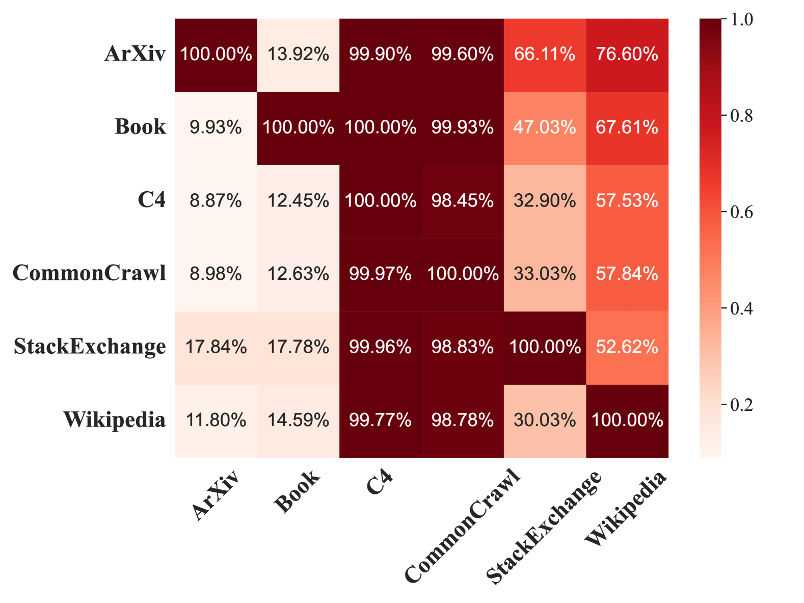
Figure 1: We conduct data clustering analysis using the SlimPajama dataset. For each domain (row), each cell shows the percentage of its clusters that also include samples from other domains (column). E.g., 76.60% of ArXiv’s clusters include Wikipedia samples (1st row, 6th column). The results reveal substantial overlap between domains.

The mixture proportions of pretraining data, which greatly affect the language model performance, have received increasing attention from researchers and practitioners. In the early years, heuristic-based methods were widely employed to assign domain weights using manually devised rules, such as upsampling high-quality datasets (e.g., Wikipedia) multiple times Gao et al. (2020); Laurençon et al. (2022). Afterwards, models like GLaM Du et al. (2022) and PaLM Chowdhery et al. (2023) established mixture weights based on the performance metrics of trained smaller models. More recently, learning-based methods have been proposed, involving the training of small proxy models across domains to generate optimal domain weights Fan et al. (2023); Xie et al. (2024). These existing methods follow a domain-wise methodology, a top-down process that first determines the proportion of each domain and then samples uniformly from the selected domain. Despite achieving advancements, These approaches present two key issues:

(1) Ignoring Inter-domain Overlaps and Commonalities. In current pretraining datasets, “domain” is primarily categorized based on data sources rather than intrinsic textual or semantic properties. An implicit assumption of the domain-wise approaches is that samples are distinct and unrelated across domain boundaries. However, in practice, samples across different domains exhibit significant shared characteristics, both in terms of raw text and high-level semantics. To examine this assumption, we analyzed the SlimPajama dataset Soboleva et al. (2023), a quality-filtered and deduplicated dataset, focusing on relationships between samples and clusters across its six text domains (excluding GitHub). For each domain, we computed the percentage of its clusters that also included samples from other domains, as Figure 1 shows. Our findings reveal substantial overlap between domains—nearly all clusters contain samples from both CommonCrawl and C4. Furthermore, manual inspection of the clustered samples confirms that data from different domains frequently share similar topics and characteristics. For instance, Figure 7 illustrates that samples from multiple domains discuss Einstein and the Theory of Relativity. By disregarding inter-domain commonalities, domain-wise mixture methods fail to control the global diversity of training data effectively.

(2) Suboptimal Sample Distribution within Domains. A second limitation arises from the uniform sampling within each domain, which can lead to a suboptimal distribution of training samples Xie et al. (2024); Fan et al. (2023); Ye et al. (2025). Intuitively, samples with higher quality and greater diversity should have a higher probability of being selected Xie et al. (2023); Abbas et al. (2023). At the same time, lower-quality samples should not be entirely discarded, as they contribute to the model’s generalization ability Sachdeva et al. (2024). Determining an effective sampling strategy within each domain is nontrivial, yet current approaches lack fine-grained control over sample selection.

To address these limitations, we propose a novel sample-wise data mixture approach with a bottom-up paradigm. Instead of defining domain proportions upfront, we first perform global sampling across the dataset based on sample quality and diversity, dynamically determining domain distributions. This allows for more precise control over the overall quality and diversity of the dataset. To implement this, we individually assess the quality and diversity of each sample and assign corresponding sampling weights based on these evaluations. Given a target token budget, we then sample each example according to its weight to construct the optimal training dataset. Also, our approach offers the additional advantage of dynamically adapting to varying token budgets, enabling the determination of optimal data proportions for each specific budget. In contrast, the vast majority of existing works rely on static data proportions, which do not adjust to different token budget constraints. The contributions of this paper are:

1. We study the problem of sample-wise pre-training data mixing, which can alleviate the limitations of overlooking inter-domain overlap and suboptimal sample distribution within domains by existing domain-wise mixing works.

2. We propose a sample-wise pre-training data mixing strategy that coordinates data quality and diversity on a per-sample basis, effectively capturing commonalities among domains and optimal sample distribution.

3. Extensive experiments on downstream tasks and perplexity evaluations demonstrate the advantages of our method. Notably, it achieves averaged baseline accuracy with 1.9x fewer training steps, highlighting its efficiency.

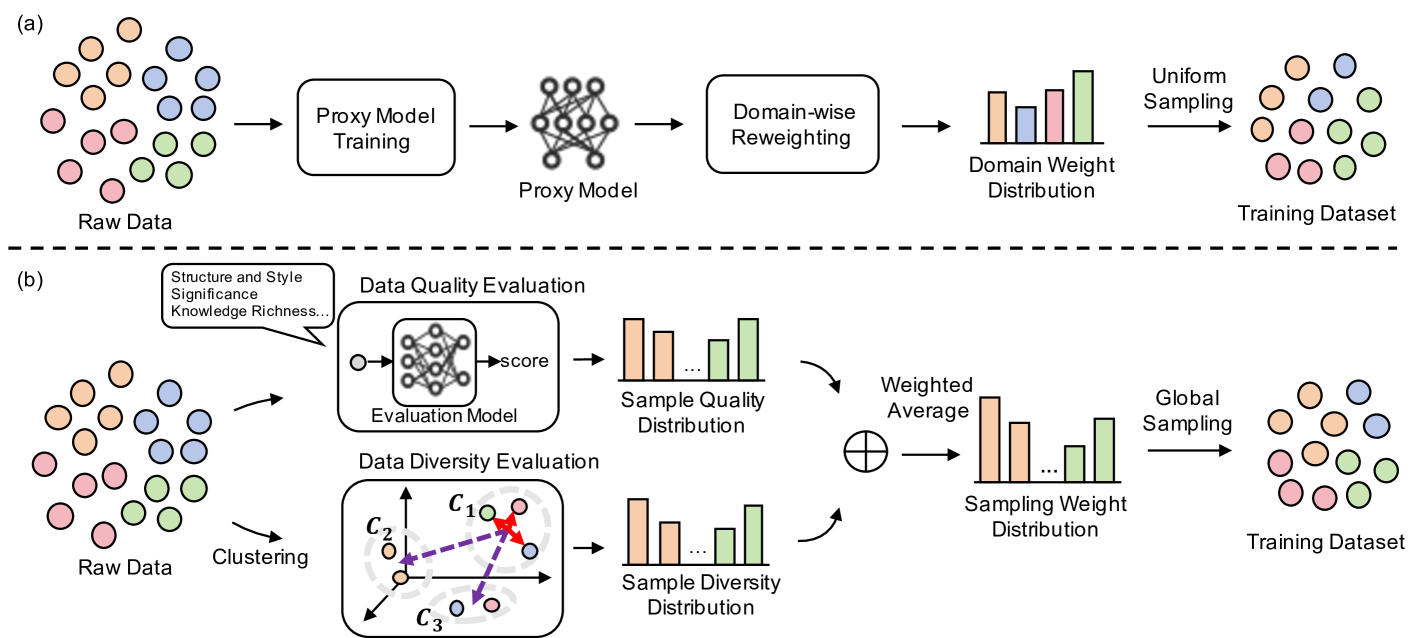
Figure 2: (a) Traditional methods determine domain weights and construct the training dataset by uniformly sampling from each domain. (b) SampleMix employs a sample-wise mixing strategy by: evaluating sample quality and diversity, assigning appropriate weights, and constructing an optimal dataset based on these weights. Dots of the same color represent data from the same domain..

2 Method

2.1 Problem Formulation

Consider a source dataset $D_{\mathrm{src}}$ composed of $k$ distinct domains (e.g., CommonCrawl, Wikipedia, BookCorpus, etc.). For each domain $i$, let $D_{i}$ denote the collection of documents within that domain. The entire source dataset is defined as $D_{\mathrm{src}}\triangleq\{D_{1},\ldots,D_{k}\}$, with $T_{\mathrm{src}}$ representing the total number of tokens. Our objective is to construct a target training set $D_{\mathrm{tgt}}$ for pre-training that adheres to a specific token budget $T_{\mathrm{tgt}}$ (e.g., 100B tokens). As illustrated in Figure 2, traditional approaches determine domain weights without explicitly considering the overall token budget, and build $D_{\mathrm{tgt}}$ by uniform sampling from each domain based on these weights. In contrast, our proposed method, SampleMix, enhances this process by evaluating both the quality (§˜2.2) and diversity (§˜2.3) of each document. Utilizing these dual criteria, SampleMix assigns unique sampling weights to each document. To ensure compliance with the token budget $T_{\mathrm{tgt}}$, we then construct an optimal training dataset by sampling documents according to their assigned weights (§˜2.4).

2.2 Data Quality Evaluation

The quality of training data is crucial for large language models. However, most existing studies typically rely on simple heuristics Xie et al. (2023); Li et al. (2023); Sachdeva et al. (2024). Wettig et al. (2024) introduces four metrics and uses pairwise comparisons to train an evaluator model. However, these metrics are applied separately in data selection, and pairwise training may neglect the objective factors that determine sample quality.

2.2.1 Quality Criteria

To comprehensively capture both the fundamental linguistic attributes and the deeper informational and analytical qualities of the text, we assert that high-quality data should adhere to the following principles: linguistic precision and clarity, structural coherence and completeness, content reliability and appropriateness, informational and educational value, as well as significance and originality. To evaluate these aspects effectively, we propose 7 quality dimensions accompanied by corresponding scores based on the aforementioned principles, as outlined in Table 1. Notably, for Knowledge Richness and Logicality and Analytical Depth, we utilize a larger scoring span {0, 1, 2} to address the wider range and greater complexity inherent in these features. By aggregating all dimension scores, we obtain an overall quality evaluation for each sample, ranging from 0 to 10.

Dimension	Score
Clarity of Expression and Accuracy	{0,1}
Completeness and Coherence	{0,1}
Structure and Style	{0,1}
Content Accuracy and Credibility	{0,1}
Significance	{0,1}
Knowledge Richness	{0,1,2}
Logicality and Analytical Depth	{0,1,2}

Table 1: Quality dimensions and scores.

2.2.2 Quality Evaluator

To develop an effective and efficient quality evaluator, we utilize GPT-4o to assess training data based on predefined quality criteria (prompt shown in Fig 10). Specifically, we uniformly sample 420k documents from the SlimPajama dataset, allocating 410k and 10k documents for train and test set respectively. We train the quality evaluator with gte-en-mlm-base model Zhang et al. (2024) as the backbone. Instead of text classification tasks, we employ ordinal regression to leverage the inherent ordering of quality scores. Following Niu et al. (2016), we transform ordinal regression into a series of binary classification problems, each indicating whether the input data exceeds a specific quality threshold. The overall quality score is then derived by subtracting the sequence of binary outputs (code shown in Appendix˜F).

Model	Text Classification	Ordinal Regression
ACC	56.14	55.94
MAE	0.77	0.72
MSE	1.95	1.57
CACC	82.24	83.37

Table 2: Performance comparison between text classification and ordinal regression models on the test set.

We evaluate the trained quality evaluator on the test set, as shown in Table 2. Instead of relying solely on Accuracy (ACC), we consider Mean Squared Error (MSE) and Mean Absolute Error (MAE), which more accurately reflect the degree of deviation between the true quality scores and the predicted results. While both the text classification and ordinal regression approaches achieve similar accuracy, the ordinal regression method demonstrates superior performance in terms of MSE and MAE. We noticed that the accuracy is lower than anticipated; detailed analysis shows that most false predictions fall within ±1 of the true quality score. To address this, we introduce Close Accuracy (CACC), a relaxed metric where a prediction is considered correct if it is within ±1 of the true quality score. The CACC results indicate that our model possesses satisfactory discriminatory ability for samples of different qualities.

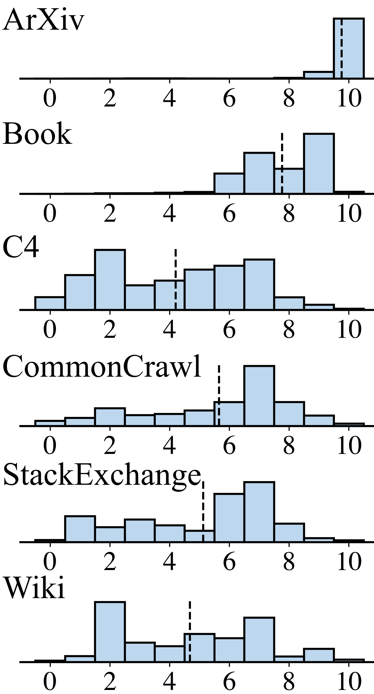
(a) Quality Distribution

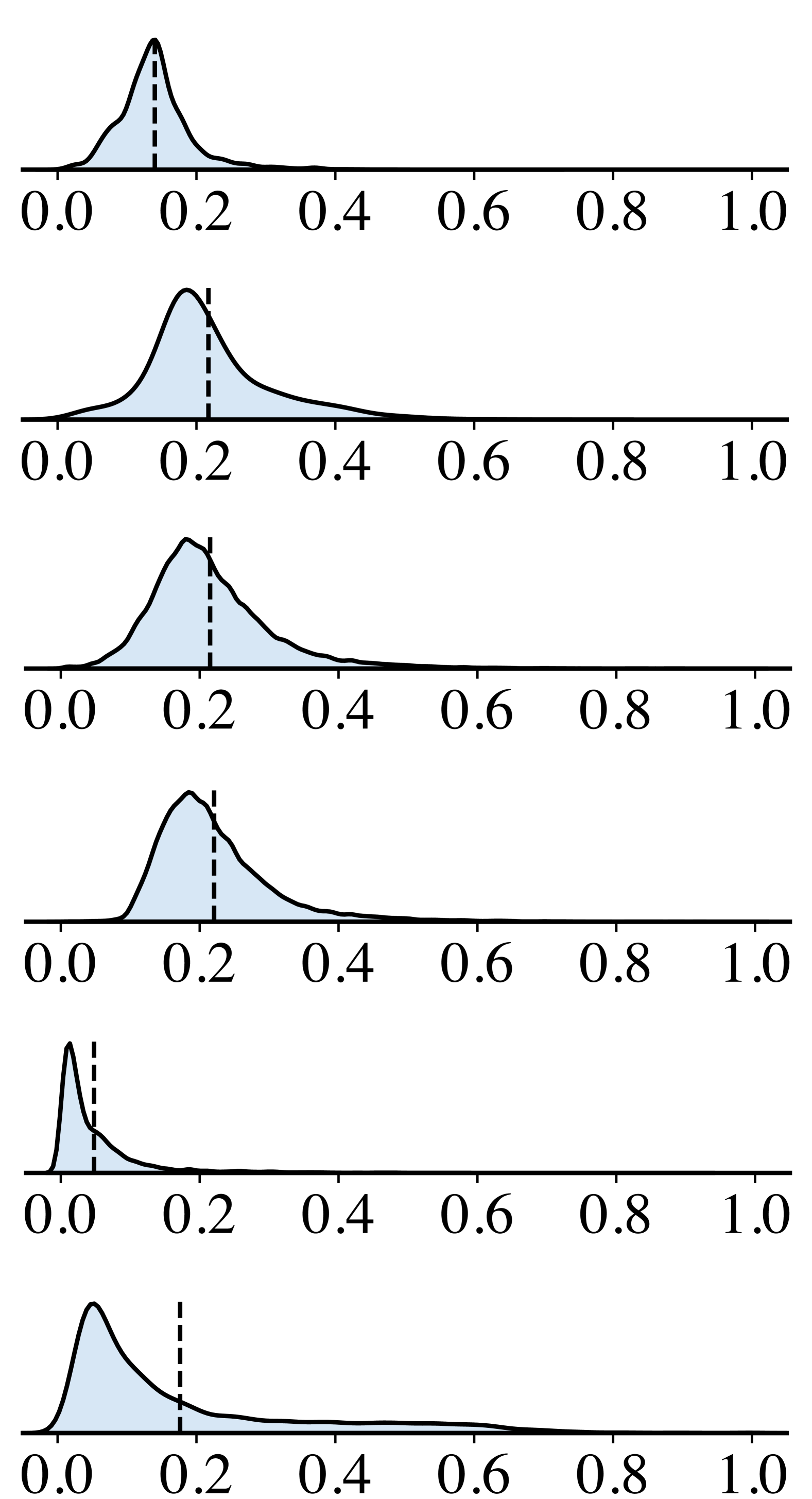
(b) Diversity Distribution

Figure 3: Analysis of SlimPajama dataset. Mean values are marked with a dashed line.

2.2.3 Analysis of Quality Distribution

Using the trained quality evaluator, we annotated the SlimPajama dataset, and the resulting quality distribution is presented in Figure 3(a), from which we can find: (1) Arxiv and Book sources exhibit higher quality, as anticipated. (2) Wikipedia is generally considered a high-quality source; however, a substantial portion is of lower quality. Our manual inspection indicates that these low-quality samples typically consist of brief, parsing errors, incomplete content, and other issues. (3) Overall, the CommonCrawl dataset outperforms C4 in terms of quality (average quality score: 5.65 v.s. 4.20).

2.3 Data Diversity Evaluation

Inspired by Shao et al. (2024a) and Abbas et al. (2024), we employ data clustering to capture the text distribution within our training dataset. Through a detailed analysis of the clustered samples, we observe patterns consistent with Abbas et al. (2024)’s work on image data, specifically: (1) Denser clusters exhibit higher similarity among their constituent samples; (2) Clusters that are proximal to others are more likely to contain samples resembling those in neighboring clusters. To quantify data diversity, we estimate a diversity measure for each sample using the Diversity Evaluator.

2.3.1 Diversity Evaluator

Data Clustering We begin by generating embeddings for each sample, which are subsequently organized into clusters via K-Means, effectively structuring the data based on textual similarity. The details of data clustering can be found in Appendix˜G.
Cluster Compactness We assess the density of a cluster by calculating the average distance of its members from the centroid, referred to as Cluster Compactness. A smaller average distance signifies a more compact cluster, indicating higher similarity among its constituent samples. This metric effectively reveals the dense property of the cluster.
Cluster Separation We evaluate the distinctiveness of each cluster by measuring the distance between its centroid and those of other clusters, termed Cluster Separation. Larger distances imply greater separation, indicating that the cluster is more distinct from others and highlighting its uniqueness on a global scale.
Data Diversity Calculation Finally, the diversity of each sample $x_{i}$ is estimated by integrating its cluster’s separation and compactness as follows:

$$d(x_{i})=d_{\text{compactness},j}\times d_{\text{separation},j}$$ (1)

where $x_{i}$ belongs to the $j$-th cluster, $d_{\text{compactness},j}$ and $d_{\text{separation},j}$ represents the cluster compactness and cluster separation for the $j$-th cluster respectively. This composite diversity measure effectively encapsulates both the homogeneity within clusters and the distinctiveness between clusters, providing a comprehensive assessment of data diversity.

2.3.2 Analysis of Diversity Distribution

We examine the diversity distribution within the SlimPajama dataset, as illustrated in Figure 3(b). We can find: (1) Within individual domains, samples’ diversity can vary significantly. For instance, the diversity distribution of C4 approximates a normal distribution, indicating consistent variability within this domain. (2) Diversity differs markedly across domains in the SlimPajama dataset. Specifically, the C4, CommonCrawl, and Book domains exhibit the highest levels of diversity, as anticipated. In contrast, the StackExchange domain demonstrates the lowest diversity among the examined domains.

2.4 Data Sampling

2.4.1 Sampling Weight Calculation

Given the quality and diversity evaluation for each document, we first min-max normalize the dual measures to ensure they lie within the interval $[0,1]$ and compute the sampling weight as follows:

$$p(x_{i})=\alpha\,d(x_{i})+(1-\alpha)\,q(x_{i})$$ (2)

where $q(x_{i})$ and $d(x_{i})$ denote quality and diversity measure of the document $x_{i}$, and $\alpha\in[0,1]$ is the weighting factor that balances the contribution of diversity relative to quality.

2.4.2 Determining Sampling Frequency

Given the source dataset $D_{\mathrm{src}}$ containing $|D_{\mathrm{src}}|$ documents with $T_{\mathrm{src}}$ tokens, we first estimate the target number of documents for $D_{\mathrm{tgt}}$ as follows:

$$|D_{\mathrm{tgt}}|=\frac{T_{\mathrm{tgt}}}{T_{\mathrm{src}}}|D_{\mathrm{src}}|$$ (3)

Then we compute each document’s sampling frequency $c(x_{i})$ using a softmax-based distribution to translate the sampling weights into probabilities:

$$c(x_{i})=|D_{\mathrm{tgt}}|\times\frac{\exp\left(p(x_{i})/\tau\right)}{\sum_{j\in D_{\mathrm{src}}}\exp\left(p(x_{i})/\tau\right)}$$ (4)

where $\tau$ is the temperature parameter that modulates the softmax distribution, controlling the concentration of the sampling probabilities.

2.4.3 Constructing the Training Dataset

Since $c(x_{i})$ typically yields non-integer values, we convert these frequencies into integer counts through the following two-step process:

• Integer Part: Always sample the document $\lfloor c(x_{i})\rfloor$ times. For example, if $c(x_{i})=2.3$, the document is sampled 2 times.

• Fractional Part: The remaining fractional part ($c(x_{i})-\lfloor c(x_{i})\rfloor$) is used to determine an additional sample probabilistically. Continuing the example, with $c(x_{i})=2.3$, there is a 30% chance that $x_{i}$ will be sampled a third time, determined by comparing the fractional part to a randomly generated number.

By aggregating the sampled counts for each document $x_{i}$, we assemble the final training dataset $D_{\mathrm{tgt}}$, which closely matches the target token budget $T_{\mathrm{tgt}}$. Our method offers key benefits: (1) Prioritization of Quality and Diversity: By incorporating both quality and diversity metrics into the sampling weights, SampleMix ensures that high-quality and diverse documents are preferentially selected, enhancing the overall effectiveness of the training dataset. (2) Adaptive to Training Budget: The sampling mechanism dynamically adjusts to different token budgets $T_{\mathrm{tgt}}$, maintaining an optimal balance between quality and diversity without the need for manual tuning. (3) Flexible Domain Representation: By allowing different sampling rates within the same domain, the method supports a more nuanced representation of various domains.

3 Experimental Setup

3.1 Dataset And Baselines

Dataset Following Xie et al. (2024); Ge et al. (2024), we experiment with the SlimPajama dataset, which consists of 7 domains from RedPajama, with intensive enhancements including NFC normalization, length filtering, and global deduplication Soboleva et al. (2023).

Baselines We compare with the following baselines: (1) Vanilla, which denotes the inherent proportions of datasets, mirroring the natural distribution patterns Soboleva et al. (2023). (2) DoReMi, which exploits a learning-based solution for multi-round mixture optimization Xie et al. (2024). (3) CE, which uses the Conditional Entropy proxy for data mixture optimization Ge et al. (2024). (4) BiMIX-OPT, which derives the optimized data mixture by the bivariate scaling law Ge et al. (2024). (5) DoGE, which determines the domain weight based on contribution to final generalization objective Fan et al. (2023). (6) DML, which derives the optimized data mixture by the data mixing law Ye et al. (2025). Note that we focus primarily on text data mixing. Following Liu et al. (2025), we exclude the GitHub domain and apply re-normalization to the baseline weights (the weights are shown in Figure 9). Investigating code data mixing remains an avenue for future research.

Benchmark	Vanilla	DoReMi	CE	BiMIX-OPT	DoGE	DML	SampleMix
Downstream Tasks Evaluation (Accuracy)
OpenBookQA	31.40	31.60	31.80	29.80	29.00	30.80	32.60
LAMBADA	38.27	40.95	42.23	38.02	37.07	35.40	40.69
PiQA	70.40	70.13	69.37	69.64	70.62	65.02	70.95
ARC-Easy	47.44	46.65	46.73	45.57	45.74	47.49	48.73
ARC-Challenge	28.58	27.30	28.33	28.33	27.65	27.73	29.86
WinoGrande	52.33	54.38	51.07	52.80	51.14	51.46	53.83
WiC	50.47	48.59	48.28	48.90	50.00	52.98	51.72
RTE	50.18	51.62	51.62	47.65	51.26	51.62	53.79
Average	46.13	46.40	46.18	45.09	45.31	45.31	47.77
Perplexity Evaluation (Perplexity)
Pile	26.93	26.45	26.20	27.47	29.49	29.76	25.63
xP3	47.38	47.08	47.62	48.74	48.38	54.00	46.38

Table 3: Comparison of data mixture methods across various downstream tasks and perplexity evaluations. The best performing method for each metric is highlighted in bold, while the second-best is underlined.

3.2 Training Setup

We train 1B-parameters LLaMA models Dubey et al. (2024) from scratch with 100B tokens. For the baselines, we uniformly sample 100B tokens based on predefined domain weights. Given that the source dataset (SlimPajama) comprises 503M documents totaling approximately 500B tokens, SampleMix generated the final training dataset consisting of 100M documents, with $\alpha$ and $\tau$ set to 0.8 and 0.2 respectively. Detailed hyperparameters, including model architecture, learning rate, and other essential settings, are provided in Table 6.

3.3 Evaluation

Downstream Task Accuracy Following Fan et al. (2023); Chen et al. (2025), we select 8 extensive downstream tasks, covering commonsense reasoning, language understanding, logical inference and general QA: OpenBookQA Mihaylov et al. (2018), LAMBADA Paperno et al. (2016), PiQA Bisk et al. (2020), ARC-Easy, ARC-Challenge Clark et al. (2018), WinoGrande Sakaguchi et al. (2021), and tasks from the SuperGLUE benchmark Wang et al. (2019). We use LM-eval Harness Gao et al. (2024) and report the 5-shot accuracy.

Validation Set Perplexity Following Ye et al. (2025), we compute perplexity on validation sets from The Pile Gao et al. (2020) to simulate separate collection of training and validation data. This metric measures the model’s ability to predict text sequences accurately across various domains, reflecting its general language modeling proficiency.

Instruction Tuning Perplexity Following Tirumala et al. (2023), we evaluate perplexity on the instruction tuning dataset xP3 Muennighoff et al. (2022) to address the high variance in downstream tasks. This evaluation gauges the model’s effectiveness in understanding and following instructions.

4 Results and Analysis

4.1 Main Results

Table 3 presents the performance comparison between the baseline methods and our proposed SampleMix across downstream tasks and perplexity evaluations. We draw the following key observations: (1) SampleMix achieves the highest average accuracy (47.77%) across the eight downstream tasks, outperforming all baseline methods. Specifically, it leads in 5 out of 8 tasks, demonstrating its efficacy in enhancing performance. (2) In perplexity evaluations, SampleMix records the lowest perplexity scores on both the Pile (25.63) and xP3 (46.38) datasets, underscoring the advantage in language modeling tasks.

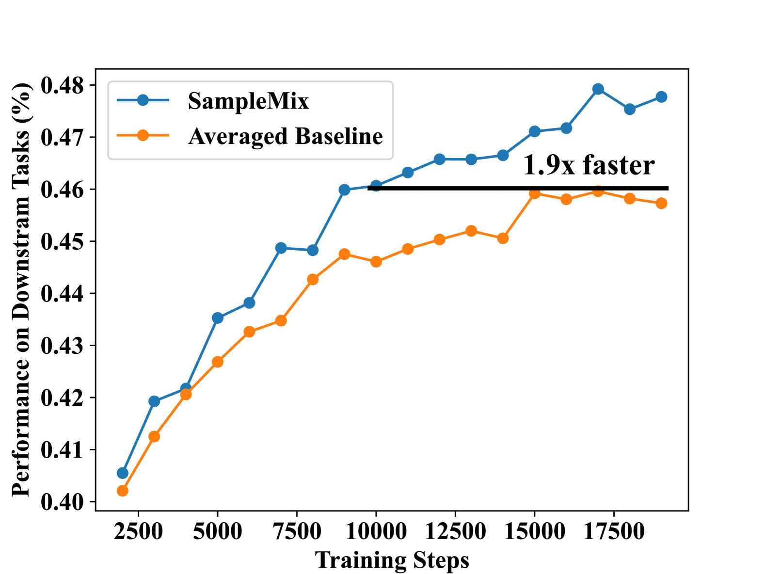
Figure 4: Training efficiency comparison. SampleMix reaches the average baseline accuracy at 100k training steps - 1.9 times faster than the averaged baselines.

Training Efficiency We compare the convergence speed of SampleMix with that of baseline methods. SampleMix achieves the baselines’ accuracy using 1.4x to 2.1x fewer training steps. As illustrated in Figure 4, it attains the average baseline accuracy within 100k steps—1.9x faster. This improvement demonstrates the efficiency gains provided by our approach. The full comparison is presented in Figure 11.

Effectiveness on larger models Furthermore, to assess the effectiveness on larger models, we trained 8B models using the top 3 performing baselines and SampleMix (training setup detailed in Table 7). As Table 4 shows, SampleMix significantly outperforms the baselines, maintaining consistent advantages observed with 1B models.

Model	Average Performance
Vanilla	53.17
DoReMi	53.58
CE	53.15
SampleMix	54.86

Table 4: Performance comparison with 8B models.

These results collectively demonstrate that SampleMix not only enhances overall performance but also does so with improved training efficiency. This establishes SampleMix as a robust and effective method for data mixture optimization.

4.2 Effectiveness of Quality and Diversity

To further explore the effectiveness of our quality and diversity evaluation, we conducted a comprehensive analysis by systematically varying the weighting factor $\alpha$. Specifically, we performed a grid search with $\alpha$ values of 0.0, 0.2, 0.4, 0.6, 0.8, and 1.0. The corresponding model performances on downstream tasks are shown in Figure 5.

From the results, we can observe the following: (1) Importance of Diversity Setting $\alpha$ to 0.0 effectively excludes the diversity measure, relying solely on quality. This configuration yields the lowest accuracy of 45.53%. As $\alpha$ increases from 0.0 to 0.8, there is a steady improvement in accuracy, peaking at 47.77%. This trend highlights the crucial role of diversity in achieving balanced data mixing and comprehensive data coverage. (2) Necessity of Quality When $\alpha$ is set to 1.0, diversity is fully weighted, and quality is excluded, leading to a slight decrease in accuracy to 47.58%. This minor drop indicates that while diversity is essential, incorporating the quality measure can further enhance performance. (3) Optimal Weighting The optimal performance at $\alpha=0.8$ illustrates that prioritizing diversity while still valuing quality leads to the most effective model performance. We attribute the results to two factors. i) Measurement Scale: The absolute value of the diversity measure is inherently smaller compared to the quality measure. Consequently, even with a higher $\alpha$, the overall influence of diversity remains balanced when integrated with quality. ii) Pre-processing Quality: The SlimPajama dataset has undergone rigorous quality filtering based on RedPajama, reducing the need for extensive weighting toward quality in the SampleMix framework. (4) Usage Recommendations Users should adjust the weighting factor $\alpha$ based on the characteristics of their datasets. For example, in datasets with inherently lower quality, prioritizing quality yields better performance.

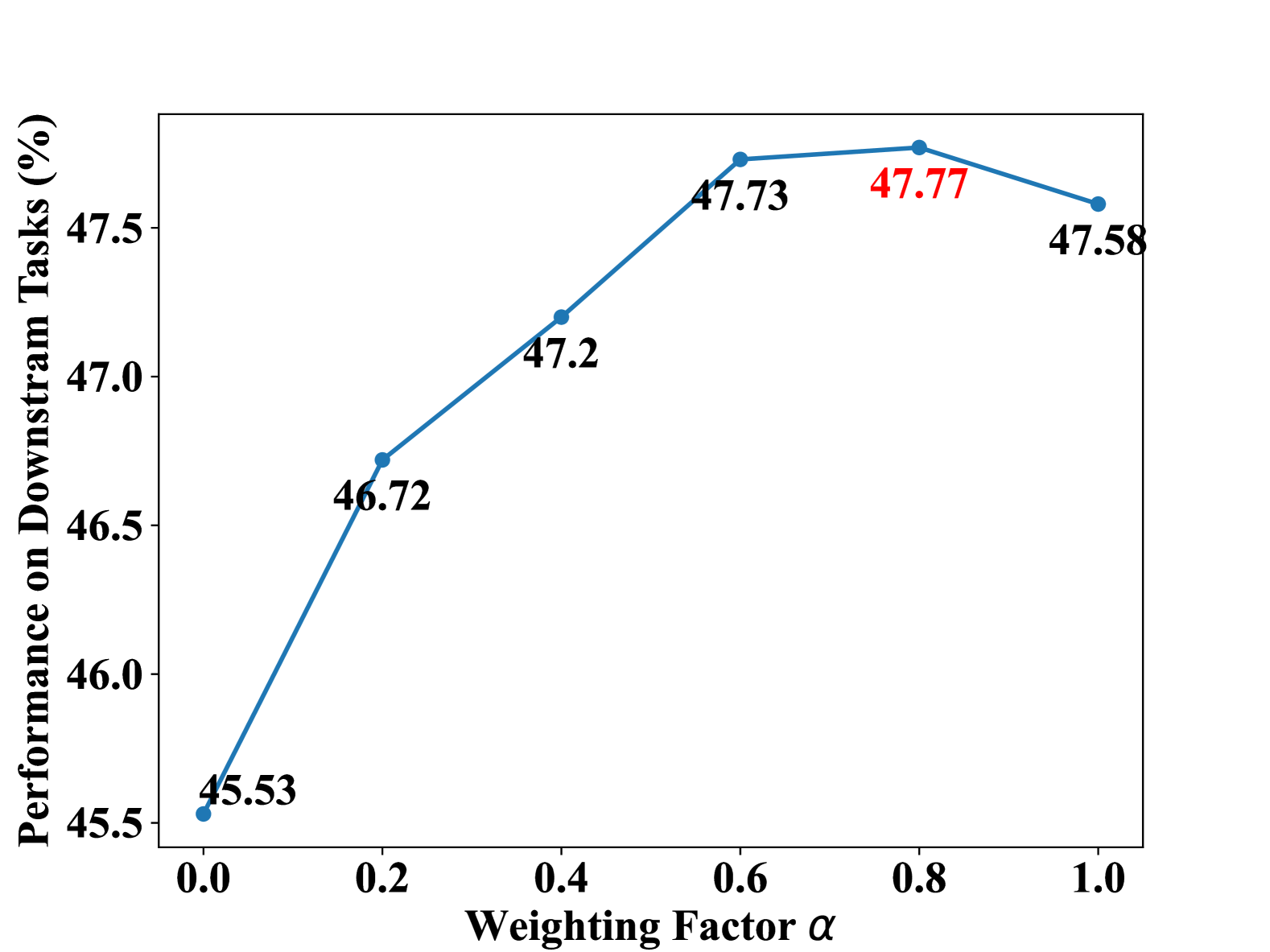
Figure 5: Average performance of downstream tasks with different weighting factor $\alpha$.

4.3 Adaptation to Varying Token Budget

Model development typically involves multiple training stages—such as pretraining, annealing, and continual pretraining—each requiring different token budgets. However, most existing methods present fixed data proportions, which limits their ability to accommodate varying token budget constraints effectively. To evaluate the benefits of dynamically adapting to different token budgets, we scale the SlimPajama dataset to $\frac{1}{5}$ of its original size, resulting in a smaller source dataset ($\approx$ 100B tokens). In our previous experiment, the full SlimPajama dataset served as the source dataset ($T_{\mathrm{src}}=500B$), while training was conducted with a subset of tokens ($T_{\mathrm{tgt}}=100B=\frac{1}{5}T_{\mathrm{src}}$). With the reduced source dataset, we adjusted the token budget proportion from $T_{\mathrm{tgt}}=\frac{1}{5}T_{\mathrm{src}}$ to $T_{\mathrm{tgt}}=T_{\mathrm{src}}$ (while maintaining $T_{\mathrm{tgt}}=100B$). We then conduct experiments under this adjusted token budget using the same setup. As Table 5 shows, we can observe that: (1) SampleMix achieves the highest average accuracy (47.46%), demonstrating SampleMix’s ability to effectively adapt to varying token budgets. (2) Baseline methods exhibit inconsistent performance when the token budget changes. For instance, DoReMi, the best-performing baseline in previous experiments, underperforms Vanilla and CE. This inconsistency indicates that baseline methods struggle to adapt effectively to different token budgets.

Model	Average Performance
Vanilla	46.65
DoReMi	46.25
CE	46.40
BiMiX-OPT	45.54
DoGE	45.01
DML	44.96
SampleMix	47.46

Table 5: Performance comparison of different data mixture methods with 100B data as candidate pool.

To further investigate how SampleMix adapts to varying token budgets, we analyze the sampling counts under different scenarios. Figure 6(a) illustrates the proportion of various sampling counts, while Figure 6(b) presents the average sampling weights $p(x)$ associated with these counts. We can observe that: For $T_{\mathrm{tgt}}=\frac{1}{5}T_{\mathrm{src}}$, the source dataset is sufficiently large, allowing top-tier data to meet the token budget. SampleMix precisely selects high-weight samples to fulfill the budget requirements, minimizing the need for extensive upsampling (i.e., sampling count > 1 is rare) and ensuring that all valuable data is included. For $T_{\mathrm{tgt}}=T_{\mathrm{src}}$, the source dataset is relatively smaller, and high-weight samples alone are insufficient to meet the token budget. To satisfy the budget, SampleMix incorporates lower-weight samples. Despite this inclusion, the method effectively identifies and discards the least valuable data, which accounts for 18.245% of the dataset due to their low sampling weights (average weight = 0.166). Data with higher sampling weights are upsampled more frequently, thereby enhancing their representation within the constrained budget. Additionally, for $T_{\mathrm{tgt}}=\frac{1}{5}T_{\mathrm{src}}$, the average sampling weight is larger (0.312 v.s. 0.289 when $T_{\mathrm{tgt}}=T_{\mathrm{src}}$), further verifying SampleMix’s ability to effectively utilize the sampling space and adapt to varying token budgets.

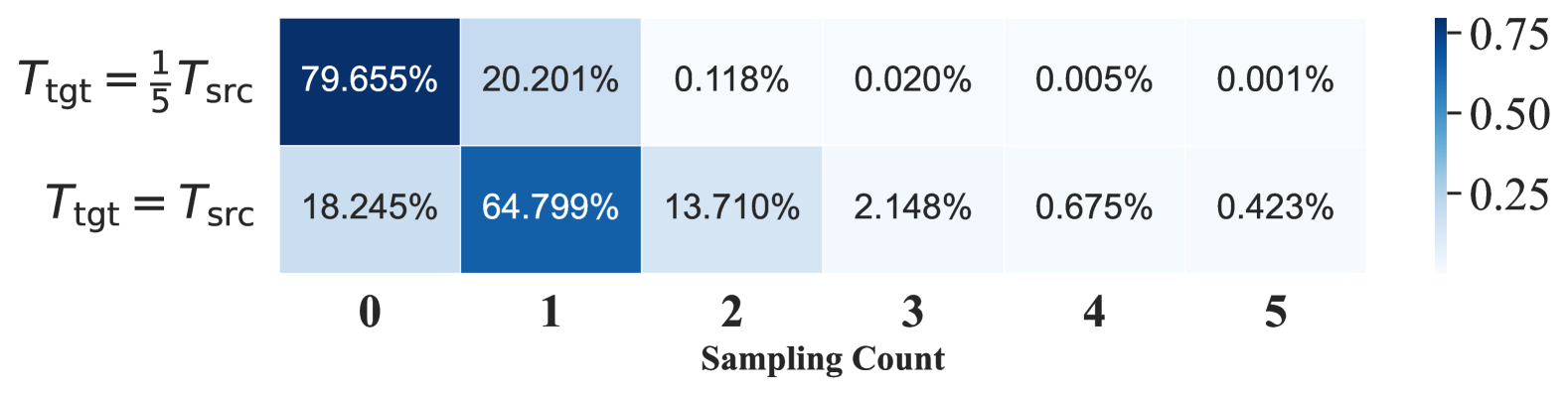
(a) Proportion of different sampling counts.

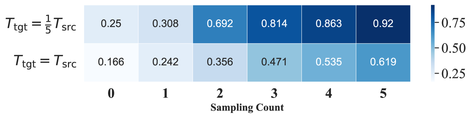
(b) Sampling weight (i.e., $p(x)$) of different sampling counts.

Figure 6: Analysis of different sampling counts.

5 Related Work

We have covered research on data mixture in §˜1, related work related to our technical designs is mainly introduced in the following.

Data Quality Heuristic rules, such as thresholds on word repetitions and perplexity, are commonly used to filter out low-quality data Yuan et al. (2021); Dodge et al. (2021); Laurençon et al. (2022) . Earlier model-based methods employ binary classifiers to distinguish high-quality from low-quality data Brown et al. (2020). Recent approaches incorporated more sophisticated models. Sachdeva et al. (2024) proposes the ASK-LLM sampler, which evaluates data quality by asking for a proxy LLM. Wettig et al. (2024) investigated four qualities-writing style, required expertise, facts & trivia, and educational value respectively. However, most methods rely on relatively coarse criteria and do not fully leverage the multi-dimensional property of data quality.

Diversity Traditional deduplication methods struggle to capture more complex semantic similarities Wenzek et al. (2020); Soldaini et al. (2024). To better handle semantic redundancy, Abbas et al. (2023) applies K-Means clustering in the embedding space to identify and remove redundant data. Tirumala et al. (2023) builds on this approach by using SemDeDup as a preprocessing step before applying SSL Prototypes Sorscher et al. (2022). Shao et al. (2024b) balances common and rare samples and ensures diversity by data clustering.

6 Conclusion

We have presented SampleMix, a sample-wise pre-training data mixing strategy by coordinating data quality and diversity. Extensive experiments demonstrate that SampleMix outperforms existing domain-wise methods, achieving comparable accuracy with 1.9x fewer training steps. In the future, we are interested in incorporating automatic evaluation metrics derived from the model’s perspective to complement the current manually designed measures, and exploring code data mixing.

7 Limitations

In this study, we conducted experiments exclusively using the SlimPajama dataset and identified the optimal hyperparameters specific to this dataset. Consequently, the hyperparameter settings reported may not directly transfer to other datasets with different characteristics. Users aiming to apply our methodology to their own datasets will need to perform tailored hyperparameter tuning to achieve optimal performance. Specifically, we suggest assigning a smaller $\alpha$ to prioritize data quality in lower-quality datasets, thereby minimizing the influence of subpar data. Conversely, for higher-quality datasets, a larger $\alpha$ is recommended to ensure comprehensive data coverage through increased diversity. However, the optimal balance between diversity and quality may vary depending on the specific attributes and complexities of different datasets.

Appendix A Domain Overlaps

We manually check the samples within the same cluster but from different domains. Such samples are usually topic-relevant and similar in terms of structure, semantics, and context. As Figure 7 shows, the samples all discuss topics about Einstein and the Theory of Relativity.

Figure 7: Samples from different domains, all describing information related to Einstein and Theory of Relativity.

Appendix B Samples from Slimpajama CommonCarwl

We manually check the low-quality and high-quality samples from Slimpajama CommonCarwl. As Figure 8 shows, the data quality of CommonCrawl varies significantly. The low-quality sample is characterized by fragmented and disorganized information, primarily consisting of sporadic headlines and links related to sports news. On the other hand, the high-quality sample provides a coherent and informative excerpt about astrophysical research, demonstrating a clear and structured narrative.

Figure 8: Quality of CommonCrawl Samples may vary significantly.

Appendix C Domain Weights of Different Methods

Figure 9 shows the domain weights of different methods.

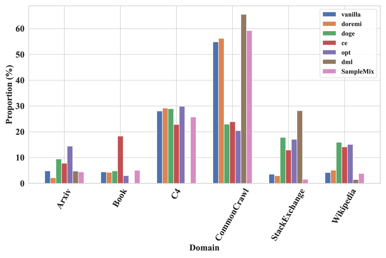
Figure 9: Domain weights of different methods.

Appendix D Hyper-Parameters of Training Models

The experiments for both 1B and 8B parameter models follow standard transformer architecture with carefully optimized hyper-parameters. Table 6 and Table 7 introduce the architectural configurations and training specifications for both model scales respectively.

Hyper-parameter	Value
layer num	28
attention head num	13
attention head dim	128
model dim	1664
ffn intermediate dim	4480
global batch size	1280
sequence length	4096
learning rate	$2e^{-4}$
learning rate scheduler	cosine scheduler
learning rate warmup tokens	525M

Table 6: Hyper-parameters of 1B models used in the experiment.

Hyper-parameter	Value
layer num	32
attention head num	32
attention head dim	128
model dim	4096
ffn intermediate dim	14336
global batch size	1280
sequence length	4096
learning rate	$2e^{-4}$
learning rate scheduler	cosine scheduler
learning rate warmup tokens	525M

Table 7: Hyper-parameters of 8B models used in the experiment.

Appendix E Quality Evaluation Prompt

The prompt for GPT-4o to assess training data quality is given in Figure 10.

Figure 10: Prompt for GPT-4o to assess training data quality.

Appendix F Code of Quality Evaluator

Table 8 shows the Python code for implementing the ordinal regression model aimed at quality scoring tasks, including model definition, loss function computation, and inference process. The full code can be found in the supplementary materials.

The OrdinalRegressionModel class initializes the pre-trained base model and a series of ordinal layers. Each ordinal layer outputs the probability that the quality score is greater than a specific threshold. For instance, the first ordinal layer (index 0) computes the probability that the quality score is greater than 0, i.e., the probability that the score is at least 1. Similarly, the second ordinal layer (index 1) calculates the probability that the quality score is greater than 1, meaning the probability that the score is at least 2, and so on. The last ordinal layer (index 9) computes the probability that the score is greater than 9, which is equivalent to the probability that the score is exactly 10. Therefore, the model has 10 ordinal layers in total, each corresponding to one of these thresholds.

The loss function calculates the ordinal loss by summing the binary cross-entropy loss between the predicted probabilities and the target values. For each ordinal layer, a binary target is created, indicating whether the true score is greater than the threshold corresponding to that layer. Specifically, the larger the deviation between the predicted score and the true score, the higher the loss, which helps the model focus on reducing these deviations during training.

The predict function implements inference using the trained ordinal regression model. It first computes the predicted probabilities for each class, and then calculates the final predicted score by selecting the class with the maximum probability. The function also calculates the probability distribution across all possible scores, which provides a measure of confidence for the predicted score.

⬇

1# Define the ordinal regression model class

2class OrdinalRegressionModel(torch.nn.Module):

3 def __init__(self, pretrained_path, num_classes=10):

4 super(OrdinalRegressionModel, self).__init__()

5 self.base_model = AutoModel.from_pretrained(pretrained_path)

6 self.ordinal_layers = torch.nn.ModuleList([torch.nn.Linear(

7 self.base_model.config.hidden_size, 1)

8 for _ in range(num_classes)])

9

10 def forward(self, input_ids, attention_mask=None, token_type_ids=None):

11 outputs = self.base_model(input_ids=input_ids,

12 attention_mask=attention_mask,

13 token_type_ids=token_type_ids)

14 last_hidden_state = outputs.last_hidden_state

15 cls_representation = last_hidden_state[:, 0, :]

16

17 # Compute the output for each ordinal layer

18 ordinal_outputs = [torch.sigmoid(layer(cls_representation))

19 for layer in self.ordinal_layers]

20 ordinal_outputs = torch.cat(ordinal_outputs, dim=1)

21 return ordinal_outputs

22

23# Calculate the ordinal loss

24def loss(outputs, targets):

25 loss = 0.0

26 for i in range(outputs.size(1)):

27 binary_targets = (targets > i).float()

28 loss += nn.functional.binary_cross_entropy(outputs[:, i], binary_targets)

29 return loss

30

31# Inference function

32def predict(text):

33 with torch.no_grad():

34 inputs = tokenizer(

35 text,

36 truncation=True,

37 padding=True,

38 max_length=4096,

39 return_tensors="pt"

40 )

41 # Get model outputs

42 outputs = model(input_ids=inputs[’input_ids’],

43 attention_mask=inputs[’attention_mask’])

44

45 # Initialize probability array

46 probabilities = torch.zeros(outputs.size(0), outputs.size(1) + 1)

47 # Calculate probability for the first class

48 probabilities[:, 0] = 1 - outputs[:, 0]

49 if outputs.size(1) > 1:

50 # Calculate probabilities for the middle classes

51 probabilities[:, 1:-1] = outputs[:, :-1] - outputs[:, 1:]

52 # Calculate probability for the last class

53 probabilities[:, -1] = outputs[:, -1]

54

55 # Calculate scores by finding the index of the maximum probability

56 scores = torch.argmax(probabilities, dim=1)

57 return scores, probabilities

Table 8: Python Code for implementing the ordinal regression model.

Appendix G K-means Clustering Details

For the data clustering in §˜2.3, we generate 768-dimensional embeddings for each sample . Further, we normalize the embeddings to have L2-norm of 1.0, and use faiss Johnson et al. (2019) to perform K-means clustering. Following Tirumala et al. (2023); Abbas et al. (2024), we set the number of clusters to be the square root of the number of total points being clustered. The core code of data clustering is presented in Table 9. The full code can be found in the supplementary materials.

⬇

1 # Calculate the number of clusters

2 n_centroids = int(math.sqrt(all_embeddings.shape[0]))

3 # define the parameters

4 kmeans = faiss.Kmeans(

5 d = 768,

6 k = n_centroids,

7 niter=50, # 50 iterations

8 gpu = True,

9 seed = 1024,

10 spherical = True,

11 min_points_per_centroid=1,

12 max_points_per_centroid=all_embeddings.shape[0]

13 )

14 # perform data clustering

15 kmeans.train(all_embeddings)

Table 9: Python Code for implementing K-Means clustering.

Appendix H Coverage Speed of All Methods

Figure 11 shows the full comparison of SampleMix and all baselines. SampleMix achieves the baselines’ accuracy using 1.4x to 2.1x fewer training steps.

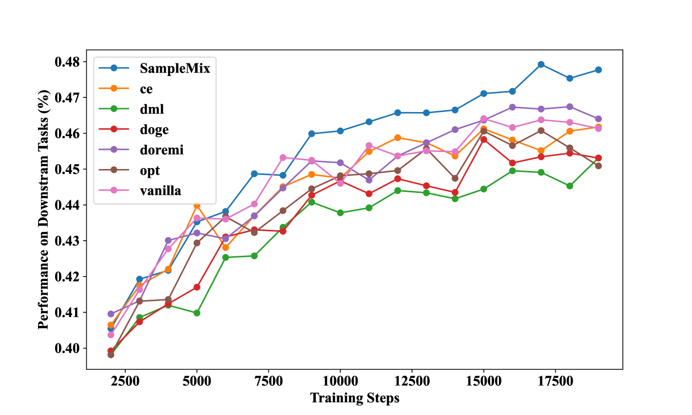
Figure 11: Coverage speed of all baselines and SampleMix. SampleMix achieves the best training efficiency.

Appendix I Analysis of Sampling Count Distribution

Figure 12(a) presents the distribution of sampling counts for each domain. Although our target training budget $T_{\mathrm{tgt}}$ is approximately equal to the size of the candidate pool $T_{\mathrm{src}}$, our method strategically discards documents with the lowest quality and diversity by assigning them a sampling count of zero. This approach contrasts with traditional methods that utilize uniform sampling across all documents. In Figure 12(b), we display the sampling weights corresponding to the sampling counts. The results demonstrate that our method allocates higher sampling counts to samplers with larger sampling weights, aligning with our expectations. Additionally, the distribution of sampling counts exhibits significant variation across different domains. This variability underscores our method’s effectiveness in capturing both fine-grained variations and commonalities among diverse domains, ensuring a more nuanced and efficient sampling process.

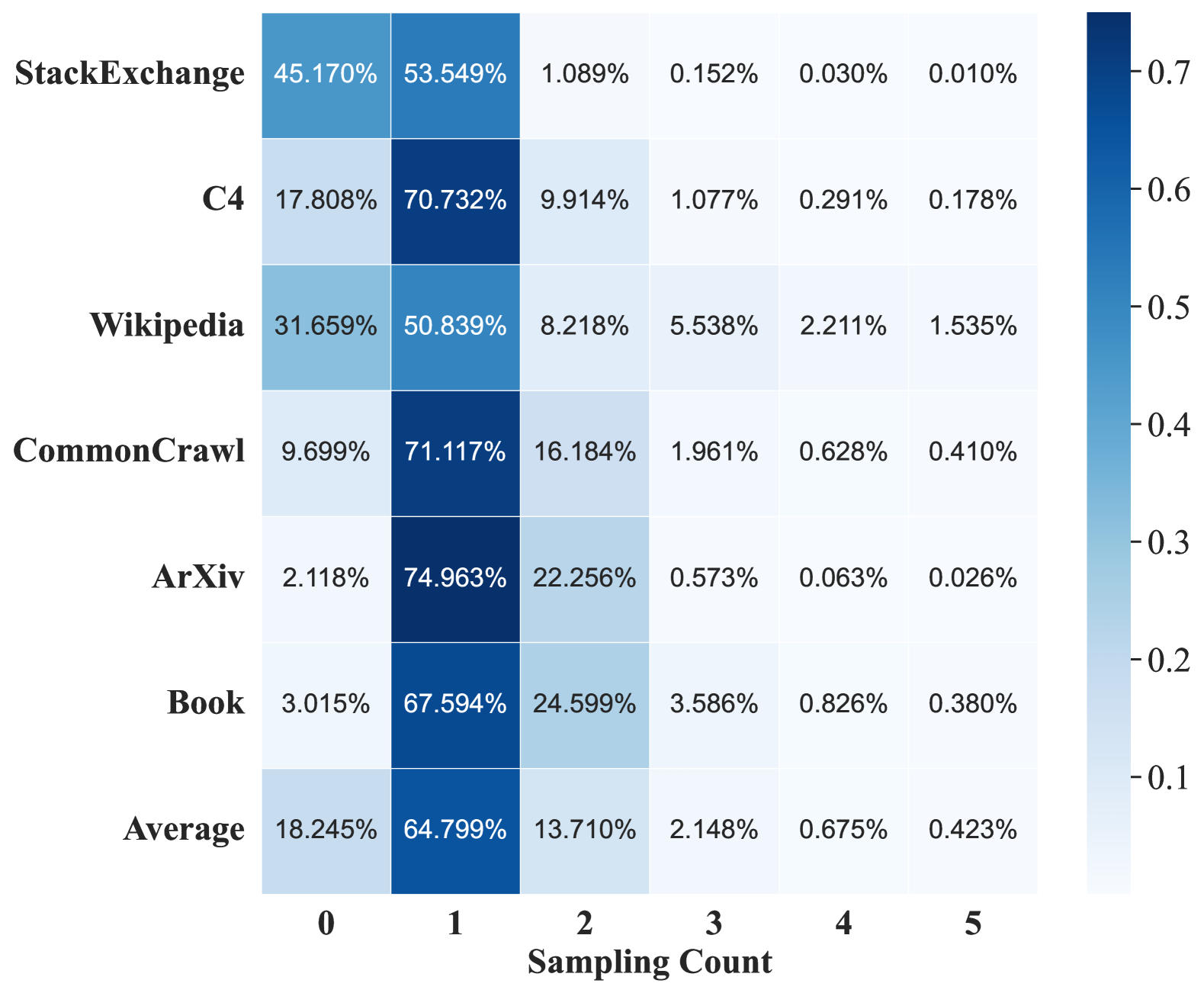
(a) Proportion of different sampling count for $T_{\mathrm{tgt}}=T_{\mathrm{src}}$

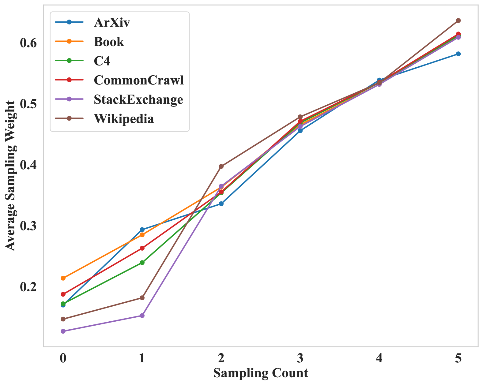
(b) Sampling weight (i.e., $p(x)$) of different sampling counts for $T_{\mathrm{tgt}}=T_{\mathrm{src}}$

Figure 12: Analysis of sampling counts.

References

- Abbas et al. (2024) Amro Abbas, Evgenia Rusak, Kushal Tirumala, Wieland Brendel, Kamalika Chaudhuri, and Ari S Morcos. 2024. Effective pruning of web-scale datasets based on complexity of concept clusters. arXiv preprint arXiv:2401.04578.
- Abbas et al. (2023) Amro Abbas, Kushal Tirumala, Dániel Simig, Surya Ganguli, and Ari S Morcos. 2023. Semdedup: Data-efficient learning at web-scale through semantic deduplication. arXiv preprint arXiv:2303.09540.
- Bisk et al. (2020) Yonatan Bisk, Rowan Zellers, Jianfeng Gao, Yejin Choi, et al. 2020. Piqa: Reasoning about physical commonsense in natural language. In Proceedings of the AAAI conference on artificial intelligence, volume 34, pages 7432–7439.
- Brown et al. (2020) Tom Brown, Benjamin Mann, Nick Ryder, Melanie Subbiah, Jared D Kaplan, Prafulla Dhariwal, Arvind Neelakantan, Pranav Shyam, Girish Sastry, Amanda Askell, et al. 2020. Language models are few-shot learners. Advances in neural information processing systems, 33:1877–1901.
- Chen et al. (2025) Mayee F Chen, Michael Y. Hu, Nicholas Lourie, Kyunghyun Cho, and Christopher Re. 2025. Aioli: A unified optimization framework for language model data mixing. In The Thirteenth International Conference on Learning Representations.
- Chowdhery et al. (2023) Aakanksha Chowdhery, Sharan Narang, Jacob Devlin, Maarten Bosma, Gaurav Mishra, Adam Roberts, Paul Barham, Hyung Won Chung, Charles Sutton, Sebastian Gehrmann, et al. 2023. Palm: Scaling language modeling with pathways. Journal of Machine Learning Research, 24(240):1–113.
- Clark et al. (2018) Peter Clark, Isaac Cowhey, Oren Etzioni, Tushar Khot, Ashish Sabharwal, Carissa Schoenick, and Oyvind Tafjord. 2018. Think you have solved question answering? try arc, the ai2 reasoning challenge. arXiv preprint arXiv:1803.05457.
- Dodge et al. (2021) Jesse Dodge, Maarten Sap, Ana Marasović, William Agnew, Gabriel Ilharco, Dirk Groeneveld, Margaret Mitchell, and Matt Gardner. 2021. Documenting large webtext corpora: A case study on the colossal clean crawled corpus. In Proceedings of the 2021 Conference on Empirical Methods in Natural Language Processing, pages 1286–1305.
- Du et al. (2022) Nan Du, Yanping Huang, Andrew M Dai, Simon Tong, Dmitry Lepikhin, Yuanzhong Xu, Maxim Krikun, Yanqi Zhou, Adams Wei Yu, Orhan Firat, et al. 2022. Glam: Efficient scaling of language models with mixture-of-experts. In International Conference on Machine Learning, pages 5547–5569. PMLR.
- Dubey et al. (2024) Abhimanyu Dubey, Abhinav Jauhri, Abhinav Pandey, Abhishek Kadian, Ahmad Al-Dahle, Aiesha Letman, Akhil Mathur, Alan Schelten, Amy Yang, Angela Fan, et al. 2024. The llama 3 herd of models. arXiv preprint arXiv:2407.21783.
- Fan et al. (2023) Simin Fan, Matteo Pagliardini, and Martin Jaggi. 2023. Doge: Domain reweighting with generalization estimation. arXiv preprint arXiv:2310.15393.
- Gao et al. (2020) Leo Gao, Stella Biderman, Sid Black, Laurence Golding, Travis Hoppe, Charles Foster, Jason Phang, Horace He, Anish Thite, Noa Nabeshima, et al. 2020. The pile: An 800gb dataset of diverse text for language modeling. arXiv preprint arXiv:2101.00027.
- Gao et al. (2024) Leo Gao, Jonathan Tow, Baber Abbasi, Stella Biderman, Sid Black, Anthony DiPofi, Charles Foster, Laurence Golding, Jeffrey Hsu, Alain Le Noac’h, Haonan Li, Kyle McDonell, Niklas Muennighoff, Chris Ociepa, Jason Phang, Laria Reynolds, Hailey Schoelkopf, Aviya Skowron, Lintang Sutawika, Eric Tang, Anish Thite, Ben Wang, Kevin Wang, and Andy Zou. 2024. A framework for few-shot language model evaluation.
- Ge et al. (2024) Ce Ge, Zhijian Ma, Daoyuan Chen, Yaliang Li, and Bolin Ding. 2024. Data mixing made efficient: A bivariate scaling law for language model pretraining. arXiv preprint arXiv:2405.14908.
- Johnson et al. (2019) Jeff Johnson, Matthijs Douze, and Hervé Jégou. 2019. Billion-scale similarity search with gpus. IEEE Transactions on Big Data, 7(3):535–547.
- Laurençon et al. (2022) Hugo Laurençon, Lucile Saulnier, Thomas Wang, Christopher Akiki, Albert Villanova del Moral, Teven Le Scao, Leandro Von Werra, Chenghao Mou, Eduardo González Ponferrada, Huu Nguyen, et al. 2022. The bigscience roots corpus: A 1.6 tb composite multilingual dataset. Advances in Neural Information Processing Systems, 35:31809–31826.
- Li et al. (2023) Yuanzhi Li, Sébastien Bubeck, Ronen Eldan, Allie Del Giorno, Suriya Gunasekar, and Yin Tat Lee. 2023. Textbooks are all you need ii: phi-1.5 technical report. arXiv preprint arXiv:2309.05463.
- Liu et al. (2025) Qian Liu, Xiaosen Zheng, Niklas Muennighoff, Guangtao Zeng, Longxu Dou, Tianyu Pang, Jing Jiang, and Min Lin. 2025. Regmix: Data mixture as regression for language model pre-training. In The Thirteenth International Conference on Learning Representations.
- Mihaylov et al. (2018) Todor Mihaylov, Peter Clark, Tushar Khot, and Ashish Sabharwal. 2018. Can a suit of armor conduct electricity? a new dataset for open book question answering. In Proceedings of the 2018 Conference on Empirical Methods in Natural Language Processing, pages 2381–2391.
- Muennighoff et al. (2022) Niklas Muennighoff, Thomas Wang, Lintang Sutawika, Adam Roberts, Stella Biderman, Teven Le Scao, M Saiful Bari, Sheng Shen, Zheng-Xin Yong, Hailey Schoelkopf, et al. 2022. Crosslingual generalization through multitask finetuning. arXiv preprint arXiv:2211.01786.
- Niu et al. (2016) Zhenxing Niu, Mo Zhou, Le Wang, Xinbo Gao, and Gang Hua. 2016. Ordinal regression with multiple output cnn for age estimation. In Proceedings of the IEEE conference on computer vision and pattern recognition, pages 4920–4928.
- Paperno et al. (2016) Denis Paperno, Germán Kruszewski, Angeliki Lazaridou, Ngoc-Quan Pham, Raffaella Bernardi, Sandro Pezzelle, Marco Baroni, Gemma Boleda, and Raquel Fernández. 2016. The lambada dataset: Word prediction requiring a broad discourse context. In Proceedings of the 54th Annual Meeting of the Association for Computational Linguistics (Volume 1: Long Papers), pages 1525–1534.
- Sachdeva et al. (2024) Noveen Sachdeva, Benjamin Coleman, Wang-Cheng Kang, Jianmo Ni, Lichan Hong, Ed H Chi, James Caverlee, Julian McAuley, and Derek Zhiyuan Cheng. 2024. How to train data-efficient llms. arXiv preprint arXiv:2402.09668.
- Sakaguchi et al. (2021) Keisuke Sakaguchi, Ronan Le Bras, Chandra Bhagavatula, and Yejin Choi. 2021. Winogrande: An adversarial winograd schema challenge at scale. Communications of the ACM, 64(9):99–106.
- Shao et al. (2024a) Yunfan Shao, Linyang Li, Zhaoye Fei, Hang Yan, Dahua Lin, and Xipeng Qiu. 2024a. Balanced data sampling for language model training with clustering. arXiv preprint arXiv:2402.14526.
- Shao et al. (2024b) Yunfan Shao, Linyang Li, Zhaoye Fei, Hang Yan, Dahua Lin, and Xipeng Qiu. 2024b. Balanced data sampling for language model training with clustering. In Findings of the Association for Computational Linguistics: ACL 2024, pages 14012–14023, Bangkok, Thailand. Association for Computational Linguistics.
- Soboleva et al. (2023) Daria Soboleva, Faisal Al-Khateeb, Robert Myers, Jacob R Steeves, Joel Hestness, and Nolan Dey. 2023. SlimPajama: A 627B token cleaned and deduplicated version of RedPajama.
- Soldaini et al. (2024) Luca Soldaini, Rodney Kinney, Akshita Bhagia, Dustin Schwenk, David Atkinson, Russell Authur, Ben Bogin, Khyathi Chandu, Jennifer Dumas, Yanai Elazar, Valentin Hofmann, Ananya Jha, Sachin Kumar, Li Lucy, Xinxi Lyu, Nathan Lambert, Ian Magnusson, Jacob Morrison, Niklas Muennighoff, Aakanksha Naik, Crystal Nam, Matthew Peters, Abhilasha Ravichander, Kyle Richardson, Zejiang Shen, Emma Strubell, Nishant Subramani, Oyvind Tafjord, Evan Walsh, Luke Zettlemoyer, Noah Smith, Hannaneh Hajishirzi, Iz Beltagy, Dirk Groeneveld, Jesse Dodge, and Kyle Lo. 2024. Dolma: an open corpus of three trillion tokens for language model pretraining research. In Proceedings of the 62nd Annual Meeting of the Association for Computational Linguistics (Volume 1: Long Papers), pages 15725–15788, Bangkok, Thailand. Association for Computational Linguistics.
- Sorscher et al. (2022) Ben Sorscher, Robert Geirhos, Shashank Shekhar, Surya Ganguli, and Ari Morcos. 2022. Beyond neural scaling laws: beating power law scaling via data pruning. Advances in Neural Information Processing Systems, 35:19523–19536.
- Tirumala et al. (2023) Kushal Tirumala, Daniel Simig, Armen Aghajanyan, and Ari Morcos. 2023. D4: Improving llm pretraining via document de-duplication and diversification. Advances in Neural Information Processing Systems, 36:53983–53995.
- Wang et al. (2019) Alex Wang, Yada Pruksachatkun, Nikita Nangia, Amanpreet Singh, Julian Michael, Felix Hill, Omer Levy, and Samuel Bowman. 2019. Superglue: A stickier benchmark for general-purpose language understanding systems. Advances in neural information processing systems, 32.
- Wenzek et al. (2020) Guillaume Wenzek, Marie-Anne Lachaux, Alexis Conneau, Vishrav Chaudhary, Francisco Guzmán, Armand Joulin, and Édouard Grave. 2020. Ccnet: Extracting high quality monolingual datasets from web crawl data. In Proceedings of the Twelfth Language Resources and Evaluation Conference, pages 4003–4012.
- Wettig et al. (2024) Alexander Wettig, Aatmik Gupta, Saumya Malik, and Danqi Chen. 2024. Qurating: Selecting high-quality data for training language models. arXiv preprint arXiv:2402.09739.
- Xie et al. (2024) Sang Michael Xie, Hieu Pham, Xuanyi Dong, Nan Du, Hanxiao Liu, Yifeng Lu, Percy S Liang, Quoc V Le, Tengyu Ma, and Adams Wei Yu. 2024. Doremi: Optimizing data mixtures speeds up language model pretraining. Advances in Neural Information Processing Systems, 36.
- Xie et al. (2023) Sang Michael Xie, Shibani Santurkar, Tengyu Ma, and Percy S Liang. 2023. Data selection for language models via importance resampling. Advances in Neural Information Processing Systems, 36:34201–34227.
- Ye et al. (2025) Jiasheng Ye, Peiju Liu, Tianxiang Sun, Jun Zhan, Yunhua Zhou, and Xipeng Qiu. 2025. Data mixing laws: Optimizing data mixtures by predicting language modeling performance. In The Thirteenth International Conference on Learning Representations.
- Yuan et al. (2021) Sha Yuan, Hanyu Zhao, Zhengxiao Du, Ming Ding, Xiao Liu, Yukuo Cen, Xu Zou, Zhilin Yang, and Jie Tang. 2021. Wudaocorpora: A super large-scale chinese corpora for pre-training language models. AI Open, 2:65–68.
- Zhang et al. (2024) Xin Zhang, Yanzhao Zhang, Dingkun Long, Wen Xie, Ziqi Dai, Jialong Tang, Huan Lin, Baosong Yang, Pengjun Xie, Fei Huang, et al. 2024. Mgte: generalized long-context text representation and reranking models for multilingual text retrieval. arXiv preprint arXiv:2407.19669.