On Noncoherent Multiple-Antenna Rayleigh Block-Fading Channels at Finite Blocklength

Abstract

This paper investigates the maximum coding rate at which data can be transmitted over a noncoherent, multiple-input, multiple-output (MIMO) Rayleigh block-fading channel using an error-correcting code of a given blocklength with a block-error probability not exceeding a given value. A high-SNR normal approximation is derived that becomes accurate as the signal-to-noise ratio (SNR) and the number of coherence intervals over which we code tend to infinity. The obtained normal approximation complements the nonasymptotic bounds that have appeared in the literature, but whose evaluation is computationally demanding. It further lays the theoretical foundation for an analytical analysis of the fundamental tradeoff between diversity, multiplexing, and channel-estimation cost at finite blocklength and finite SNR.

I Introduction

There exists an increasing interest in the problem of transmitting short packets in wireless communications [1]. For example, the vast majority of wireless connections in the next generations of cellular systems will most likely be originated by autonomous machines and devices, which predominantly exchange short packets. It is also expected that enhanced mobile-broadband services will be complemented by new services that target systems requiring reliable real-time communication with stringent requirements on latency and reliability. While capacity and outage capacity provide accurate benchmarks for the throughput achievable in wireless communication systems when the package length is not restricted, for short-package wireless communications, a more refined analysis of the maximum coding rate as a function of the blocklength is needed. Such an analysis is provided in this paper.

Let $R^{\ast}(n,\epsilon)$ denote the maximum coding rate at which data can be transmitted using an error-correcting code of blocklength $n$ with a block-error probability no larger than $\epsilon$. Hayashi [2] and Polyanskiy, Poor, and Verdú [3] showed that for various channels with a positive capacity $C$, $R^{\ast}(n,\epsilon)$ can be tightly approximated as

$$R^{\ast}(n,\epsilon)=C-\sqrt{\frac{V}{n}}Q^{-1}(\epsilon)+\mathcal{O}\left(\frac{\log n}{n}\right)$$ (1)

where $V$ is the so-called channel dispersion; $Q^{-1}(\epsilon)$ denotes the inverse of the Q-function

$$Q(x)\triangleq\frac{1}{\sqrt{2\pi}}\int_{x}^{\infty}e^{-t^{2}/2}\mathrm{d}t$$ (2)

and $\mathcal{O}(\log n/n)$ comprises terms that decay no slower than $\log n/n$. The approximation that follows by ignoring the $\mathcal{O}(\log n/n)$ term is sometimes referred to as normal approximation. The normal approximation has been established as a benchmark for short error-correcting codes; see, e.g., [4, 5]. It further serves as a proxy for the maximum coding rate in the analysis and optimization of communication systems that exchange short packets and has appeared in numerous papers on short-packet wireless communications; see, e.g., [6, 7, 8, 9, 10, 11, 12, 13, 14, 15]. However, many of these works consider the normal approximation of the Gaussian channel, which may fail to capture the effects of key parameters in wireless communication systems, such as coherence time, diversity, or multiplexing gain.

To address this shortcoming, the work of Polyanskiy et al. has been generalized to several wireless communication channels [16, 17, 18, 19, 20, 21, 22, 23, 24, 25, 26, 27]. In particular, the channel dispersion of coherent fading channels, where the receiver has perfect knowledge of the realizations of the fading coefficients, was obtained by Polyanskiy and Verdú for the single-antenna case [16], and by Collins and Polyanskiy for the multiple-input single-output (MISO) [17] and the multiple-input multiple-output (MIMO) case [18, 19]. The case where the number of transmit and receive antennas grows with the blocklength was considered in [20]. When both the transmitter and the receive have perfect knowledge of the realization of the fading coefficients and the transmitter satisfies a long-term power constraint, the channel dispersion of single-antenna quasi-static fading channels was obtained by Yang et al. [21]. In the non-coherent setting, the channel dispersion is only known in the quasi-static case, where it is zero [22]. For general non-coherent Rayleigh block-fading channels, non-asymptotic bounds on the maximum coding rate were presented in [23] and [24]. Saddlepoint approximations that accurately approximate these bounds in the single-antenna case with a negligible computational cost were given in [25, 26]. However, a closed-form expression of the channel dispersion for general non-coherent Rayleigh block-fading channels is still unknown. Obtaining such an expression is difficult because the capacity-achieving input distribution is in general unknown. Thus, the standard approach of obtaining expressions of the form (1), which consists of first evaluating nonasymptotic upper and lower bounds on $R^{\ast}(n,\epsilon)$ for the capacity-achieving input and output distributions and then analyzing these bounds in the limit as $n\to\infty$, cannot be followed. Fortunately, the asymptotic behavior of the capacity of such channels at high signal-to-noise ratio (SNR) is well understood [28, 29]. This fact was exploited in [27] to derive a high-SNR normal approximation of $R^{\ast}(n,\epsilon)$ for non-coherent single-antenna Rayleigh block-fading channels.

In this paper, we generalize [27] to the MIMO case. In particular, we present an expression of $R^{\ast}(n,\epsilon)$ similar to (1) for non-coherent MIMO Rayleigh block-fading channels. By deriving asymptotically-tight approximations of the capacity and the channel dispersion at high SNR, we obtain a high-SNR normal approximation of $R^{\ast}(n,\epsilon)$, which complements the existing non-asymptotic bounds.

The rest of the paper is organized as follows. Section II introduces the system model. Section III presents and discusses the main result of this paper: a high-SNR normal approximation for noncoherent MIMO block-fading channels that becomes accurate As the SNR and the number of coherence intervals over which we code tend to infinity. The proof of the main result is given in Section IV. The paper concludes with a summary and discussion of our results in Section V. Some of the proofs are deferred to the appendices.

Notation

Upper-case letters such as $X$ denote scalar random variables and their realizations are written in lower case, e.g., $x$. We use boldface upper-case letters to denote random matrices, e.g., $\mathbf{X}$, and upper-case letters of a special font for their realizations, e.g., $\mathsf{X}$. The distribution of a circularly-symmetric complex Gaussian random variable with mean $\mu$ and variance $\sigma^{2}$ is denoted by $\mathcal{CN}(\mu,\sigma^{2})$. The Gamma distribution of shape parameter $\alpha$ and rate parameter $\lambda$ is denoted by $\Gamma(\alpha,\lambda)$. We use $\mathsf{E}[\cdot]$ and $\mathrm{Var}(\cdot)$ to denote expectation and variance, respectively. The symbol “$\stackrel{{\scriptstyle d}}{{=}}$" indicates equivalence in distribution.

We write $(\cdot)^{\mathsf{H}}$, $(\cdot)^{\ast}$, and $(\cdot)^{\mathsf{T}}$ to denote Hermitian transposition, complex conjugation, and transpose (without conjugation), respectively, and $\text{tr}(\cdot)$ and $\det(\cdot)$ to denote the trace and the determinant, respectively. The identity matrix of size $a\times a$ is written as $\mathsf{I}_{a}$, and $\text{diag}\{d_{1},\ldots,d_{a}\}$ denotes an $(a\times a)$-dimensional diagonal matrix with entries $d_{1},\ldots,d_{a}$. The submatrix that is composed of the first $i$ columns and rows of a matrix $\mathsf{X}$ is denoted as $[\mathsf{X}]_{(1:i)^{2}}$. For any matrix $\mathsf{X}$, $\|\mathsf{X}\|_{\textnormal{F}}$ denotes the Frobenius norm.

Throughout the paper, $\log(\cdot)$ denotes the natural logarithm function, $[a]^{+}$ stands for $\max\{a,0\}$, and $\mathds{1}\{\cdot\}$ denotes the indicator function. We shall further use the following Gamma and digamma functions:

$$\Gamma(x) \triangleq \int_{0}^{\infty}t^{x-1}e^{-t}\textnormal{d}t,\quad$$ Gamma function

$$\Gamma_{m}(x) \triangleq \pi^{m(m-1)/2}\prod_{k=1}^{m}\Gamma(x-k+1),\quad$$ complex multivariate Gamma function

$$\varPsi(x) \triangleq \frac{\textnormal{d}}{\textnormal{d}x}\log\Gamma(x),\quad$$ Euler’s digamma function

$$\varPsi^{\prime}(x) \triangleq \frac{\textnormal{d}}{\textnormal{d}x}\varPsi(x),\quad \varPsi(\cdot)$$ derivative of .

Last but not least, we denote by $\varlimsup$ the limit superior and by $\varliminf$ the limit inferior.

II System Model

We consider a Rayleigh block-fading channel with $n_{t}$ transmit antennas, $n_{r}$ receive antennas, and coherence interval $T$. For this channel, within the $\ell$-th coherence interval, the channel input-output relation is given by

$$\mathbf{Y}_{\ell}=\mathbf{X}_{\ell}\mathbf{H}_{\ell}+\mathbf{W}_{\ell}$$ (3)

where $\mathbf{X}_{\ell}$ is the complex-valued, $(T\times n_{t})$-dimensional, transmitted matrix; $\mathbf{Y}_{\ell}$ is the complex-valued, $(T\times n_{r})$-dimensional, received matrix; $\mathbf{H}_{\ell}$ is the complex-valued, $(n_{t}\times n_{r})$-dimensional fading matrix with independent and identically distributed (i.i.d.) $\mathcal{CN}(0,1)$ entries; $\mathbf{W}_{\ell}$ is the complex-valued, $(T\times n_{r})$-dimensional, additive noise at the receiver with i.i.d. $\mathcal{CN}(0,1)$ entries. We assume that $\mathbf{H}_{\ell}$ and $\mathbf{W}_{\ell}$ are independent and take on independent realizations over successive coherence intervals. We further assume that the joint law of $\mathbf{H}_{\ell}$ and $\mathbf{W}_{\ell}$ does not depend on $\mathbf{X}_{\ell}$. We consider a non-coherent setting where transmitter and receiver only know the statistics of the fading matrix $\mathbf{H}_{\ell}$ but do not have a priori knowledge of its realization.

We assume that $n_{t}\leq n_{r}$ and $T\geq n_{t}+n_{r}$. The assumption $n_{t}\leq n_{r}$ incurs no loss in capacity at high SNR [28]. More specifically, Zheng and Tse [28] showed that, at high SNR, the capacity of the non-coherent Rayleigh block-fading channel can be expressed as

$$C(\rho)=n_{\star}\left(1-\frac{n_{\star}}{T}\right)\log(\rho)+\mathcal{O}_{\rho}(1)$$

where $n_{\star}\triangleq\min\{n_{t},n_{r},\lfloor T/2\rfloor\}$ and $\mathcal{O}_{\rho}(1)$ summarizes terms that are bounded in the SNR $\rho$. This implies that, for a given coherence time $T$ and number of receive antennas $n_{r}$, the capacity pre-log is maximized by using $n_{t}=\min\{n_{r},\lfloor T/2\rfloor\}$ transmit antennas. Thus, using more than $n_{r}$ transmit antennas does not increase the high-SNR capacity. The assumption $T\geq n_{t}+n_{r}$ is reasonable for slow-fading channels when the number of antennas is moderate. Under this assumption, an input distribution referred to as unitary space-time modulation (USTM) achieves a lower bound on the capacity that is asymptotically tight in the limit as the SNR tends to infinity [28, 29]. When $T<n_{t}+n_{r}$, USTM inputs are no longer optimal and an input distribution called beta-variate space-time modulation (BSTM) should be considered instead [29]. Analyzing the maximum coding rate for this input distribution requires a different analysis that is beyond the scope of this paper.

For simplicity, we shall restrict ourselves to codes whose blocklength is $n=LT$, where $L$ denotes the number of blocks of coherence interval $T$ a codeword spans. An $(L,T,M,\epsilon,\rho)$ code consists of:

• An encoder $f$: $\{1,\cdots,M\}\rightarrow(\mathbb{C}^{T\times n_{t}})^{L}$ that maps a message $A$, which is uniformly distributed on $\{1,\cdots,M\}$, to a codeword $\mathbf{X}^{L}=[\mathbf{X}_{1},\cdots,\mathbf{X}_{L}]$. The codewords are assumed to satisfy the power constraint

  $$\|\mathbf{X}_{\ell}\|_{\textnormal{F}}^{2}\leq T\rho,\quad\ell=1,\cdots,L,\,\textnormal{with probability one.}$$ (4)

  Since the variances of $\mathbf{H}_{\ell}$ and $\mathbf{W}_{\ell}$ are normalized, $\rho$ can be interpreted as the average SNR at the receiver.

• A decoder $g$: $(\mathbb{C}^{T\times n_{t}})^{L}\rightarrow\{1,\cdots,M\}$ satisfying the maximum error probability constraint

  $$\max_{1\leq a\leq M}\Pr\big{[}g(\mathbf{Y}^{L})\neq A|A=a\big{]}\leq\epsilon$$

  where $\mathbf{Y}^{L}=[\mathbf{Y}_{1},\cdots,\mathbf{Y}_{L}]$ is the channel output induced by the codeword $\mathbf{X}^{L}=f(a)$, according to (3).

The maximum coding rate is defined as

$$R^{\ast}(L,T,\epsilon,\rho)\triangleq\sup\left\{\frac{\ln M}{LT}:\exists(L,T,M,\epsilon,\rho)\text{ code}\right\}.$$ (5)

III Main Results

The main result of this paper is a high-SNR normal approximation of $R^{\ast}(L,T,\epsilon,\rho)$ presented in Section III-A. In Section III-B, we discuss the accuracy of this approximation by means of numerical results. Possible applications are discussed in Section III-C.

III-A High-SNR Normal Approximation

Theorem 1

Assume that $T\geq n_{r}+n_{t}$, $n_{r}\geq n_{t}$, and $0<\epsilon<\frac{1}{2}$. Then, at high SNR,

$$R^{\ast}(L,T,\epsilon,\rho) = \tilde{I}(T,\rho)+K_{\tilde{I}}(T,\rho)-\sqrt{\frac{\tilde{V}(T)+K_{\tilde{V}}(T,\rho)}{L}}Q^{-1}(\epsilon)+K_{L}(L,T,\rho)$$ (6)

where

$$\tilde{I}(T,\rho) \triangleq n_{t}\left(1-\frac{n_{t}}{T}\right)\log\left(\frac{\rho}{n_{t}}\right)+n_{t}\left(1-\frac{n_{t}}{T}\right)\log\left(\frac{T}{e}\right)+\frac{1}{T}\log\frac{\Gamma_{n_{t}}(n_{t})}{\Gamma_{n_{t}}(T)}+\left(1-\frac{n_{t}}{T}\right)\sum_{i=0}^{n_{t}-1}\varPsi(n_{r}-i)$$ (7)

$$\tilde{V}(T) \triangleq \frac{n_{t}}{T}\left(1-\frac{n_{t}}{T}\right)+\left(1-\frac{n_{t}}{T}\right)^{2}\sum_{i=0}^{n_{t}-1}\varPsi^{\prime}(n_{r}-i).$$ (8)

In (6), $K_{\tilde{I}}(T,\rho)$ and $K_{\tilde{V}}(T,\rho)$ are functions of $T$ and $\rho$ which satisfy

$$\lim_{\rho\to\infty}K_{\xi}(T,\rho)=0,\quad\xi\in\{\tilde{I},\tilde{V}\}$$ (9)

and $K_{L}(L,T,\rho)$ is a function of $L$, $T$, and $\rho$ which satisfies

$$\sup_{\rho\geq\rho_{0}}\big{|}K_{L}(L,T,\rho)\big{|}\leq A\frac{\log L}{L},\quad L\geq L_{0}$$ (10)

for some $A$, $L_{0}$, and $\rho_{0}$ independent of $L$ and $\rho$.

Proof:

See Sec. IV. ∎

The quantity $\tilde{I}(T,\rho)$ is an asymptotically-tight lower bound on the capacity $C(\rho)$ of the non-coherent MIMO Rayleigh block-fading channel [29]. Similarly, $\tilde{V}(T)$ can be viewed as a high-SNR approximation of the channel dispersion. By ignoring the error terms $K_{\tilde{I}}(T,\rho)$, $K_{\tilde{V}}(T,\rho)$, and $K_{L}(L,T,\rho)$ in (6), we obtain the high-SNR normal approximation

$$R^{\ast}(L,T,\epsilon,\rho)\approx\tilde{I}(T,\rho)-\sqrt{\frac{\tilde{V}(T)}{L}}Q^{-1}(\epsilon).$$ (11)

Observe that $\tilde{I}(T,\rho)$ and $\tilde{V}(T)$ depend on $n_{r}$ only via the digamma function $\varPsi(n_{r}-i)$ and its derivative $\varPsi^{\prime}(n_{r}-i)$, respectively. On the domain of positive integers, the digamma function is monotonically increasing, and its derivative is monotonically decreasing. As a consequence, the approximation (11) is monotonically increasing in $n_{r}$. As we shall observe in Section III-B, the dependence of (11) on $n_{t}$ is more intricate. Intuitively, increasing the number of transmit antennas achieves a higher the multiplexing gain $\min\{n_{t},n_{r}\}$, but it also requires the estimation of more channel coefficients.

For comparison, at high SNR, the capacity $C_{c}(\rho)$ of the coherent MIMO Rayleigh block-fading channel satisfies [30]

$$\lim_{\rho\to\infty}\left\{C_{c}(\rho)-n_{t}\log\left(\frac{\rho}{n_{t}}\right)-\mathsf{E}\left[\log\det(\mathbf{H}_{\ell}\mathbf{H}_{\ell}^{\mathsf{H}})\right]\right\}=0.$$ (12)

Furthermore, the channel dispersion $V_{c}(\rho)$ converges to [19]

$$\lim_{\rho\to\infty}V_{c}(\rho)=\frac{n_{t}}{T}+\mathrm{Var}\bigl{(}\log\det(\mathbf{H}_{\ell}\mathbf{H}_{\ell}^{\mathsf{H}})\bigr{)}.$$ (13)

Applying [31, Lemma A.2] to (7) and (8), the high-SNR capacity and dispersion of the noncoherent block-fading channel can be written as

$$\tilde{I}(T,\rho) = n_{t}\left(1-\frac{n_{t}}{T}\right)\log\left(\frac{\rho}{n_{t}}\right)+\left(1-\frac{n_{t}}{T}\right)\mathsf{E}\left[\log\det(\mathbf{H}_{\ell}\mathbf{H}_{\ell}^{\mathsf{H}})\right]$$ (14)

$${}+n_{t}\left(1-\frac{n_{t}}{T}\right)\log\left(\frac{T}{e}\right)+\frac{1}{T}\log\frac{\Gamma_{n_{t}}(n_{t})}{\Gamma_{n_{t}}(T)}$$

and

$$\tilde{V}(T)=\left(1-\frac{n_{t}}{T}\right)\frac{n_{t}}{T}+\left(1-\frac{n_{t}}{T}\right)^{2}\mathrm{Var}\bigl{(}\log\det(\mathbf{H}_{\ell}\mathbf{H}_{\ell}^{\mathsf{H}})\bigr{)}.$$ (15)

Observe that, up to SNR-independent terms, $\tilde{I}(T,\rho)$ is given by $(1-n_{t}/T)$ times the high-SNR approximation of $C_{c}(\rho)$. Similarly, $\tilde{V}(T)$ corresponds to the high-SNR channel dispersion one obtains by transmitting in each coherence block one pilot symbol per transmit antenna to estimate the fading coefficient, and by then transmitting $T-n_{t}$ symbols over a coherent fading channel. This suggests the heuristic that, at high SNR, one pilot symbol per transmit antenna should be transmitted in each coherence block followed by coherent transmission. However, this heuristic may be misleading, since the SNR-independent terms of $\tilde{I}(T,\rho)$ may be significant, and since it is prima facie unclear whether one pilot symbol per transmit antenna and coherence block suffices to obtain a fading estimate of sufficient accuracy. For the single-antenna case, a more refined analysis of the maximum coding rate achievable with pilot-assisted transmission can be found in [32].

III-B Numerical Results

We next provide numerical examples that illustrate the accuracy of the high-SNR normal approximation in Theorem 1. In the following figures, we depict the high-SNR normal approximation (6), the normal approximation of the coherent MIMO Rayleigh block-fading channel obtained in [19], a non-asymptotic (in $\rho$ and $L$) lower bound on $R^{\ast}(L,T,\epsilon,\rho)$ that is based on the dependence testing (DT) bound, and a non-asymptotic upper bound that is based on the meta converse (MC) bound obtained in [24]. The non-asymptotic bounds are both evaluated using the communication toolbox SPECTRE [33]. In these figures, the shaded area indicates the area where $R^{\ast}(L,T,\epsilon,\rho)$ lies.

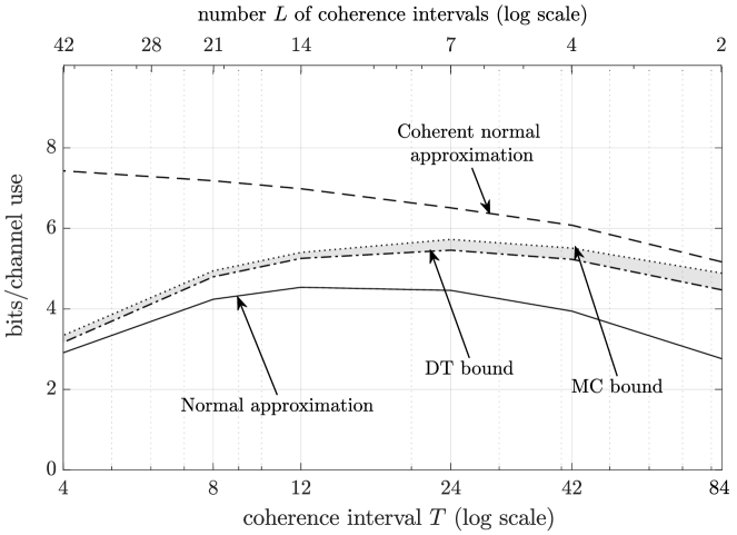
(a) $n=168$, $\epsilon=10^{-3}$, $\rho=15$ dB, and $n_{t}=n_{r}=2$.

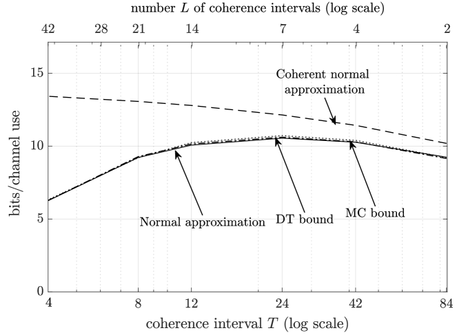
(b) $n=168$, $\epsilon=10^{-3}$, $\rho=25$ dB, and $n_{t}=n_{r}=2$.

Figure 1: $R^{*}(L,T,\epsilon,\rho)$ as a function of $T$ for a fixed $n=TL$.

In Figs. 1a and 1b, we show $R^{\ast}(L,T,\epsilon,\rho)$ as a function of $T$ for a fixed blocklength $n=LT=168$ for and the SNR values $\rho=15$ dB and $\rho=25$ dB. Observe that the high-SNR normal approximation (6) accurately describes the maximum coding rate for $\rho=25$ dB but is loose for $\rho=15$ dB unless $L$ is large. Furthermore, as expected, the normal approximation of the coherent setting is strictly larger than that of the non-coherent setting, and it becomes more accurate as $T$ increases, indicating that the cost for estimating the channel decreases with $T$.

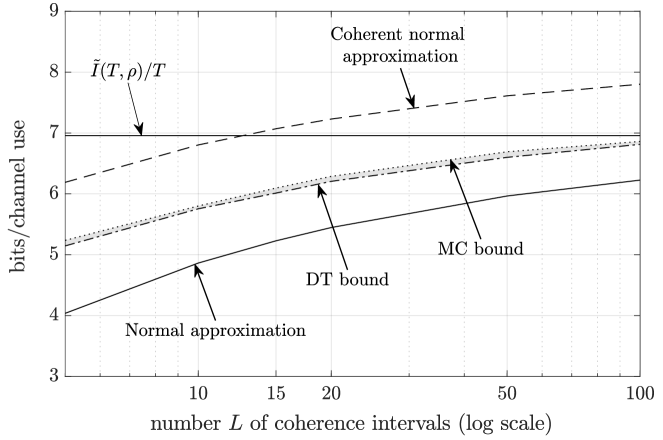
(a) $T=24$, $\epsilon=10^{-3}$, $n_{t}=2,n_{r}=2$, and $\rho=15$ dB.

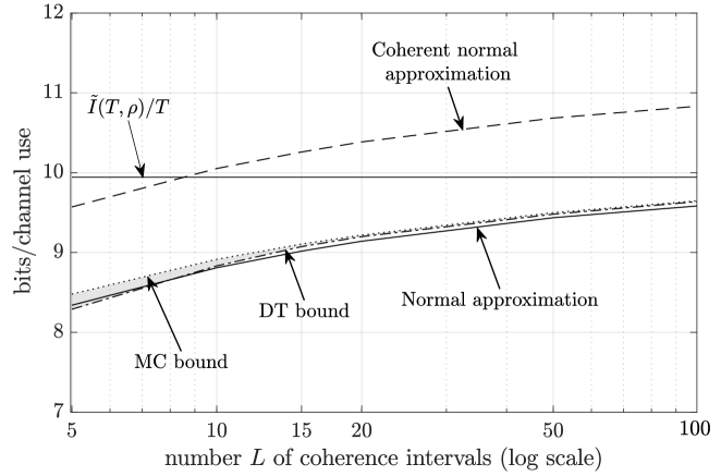
(b) $T=24$, $\epsilon=10^{-3}$, $n_{t}=2,n_{r}=4$, and $\rho=15$ dB.

Figure 2: $R^{\ast}(L,T,\epsilon,\rho)$ as a function of $n$ for a fixed $T$.

In Figs. 2a and 2b, we show $R^{\ast}(L,T,\epsilon,\rho)$ as a function of the blocklength $n=LT$ for $T=24$ and $\rho=15$ dB, and for $n_{t}=n_{r}=2$, and $n_{t}=2,n_{r}=4$, respectively. For comparison, we further depict $\tilde{I}(T,\rho)$ (7), which is an asymptotically tight lower bound on capacity. Observe that the normal approximation (6) becomes more accurate as $L$ and $n_{r}$ increase, and for $n_{r}=4$, it is very close to the non-asymptotic bounds for the considered values of $L$. Moreover, the gap between the coherent and the non-coherent normal approximations appears to be independent of $L$. This agrees with the intuition that the cost for estimating the channel is determined by the coherence interval $T$.

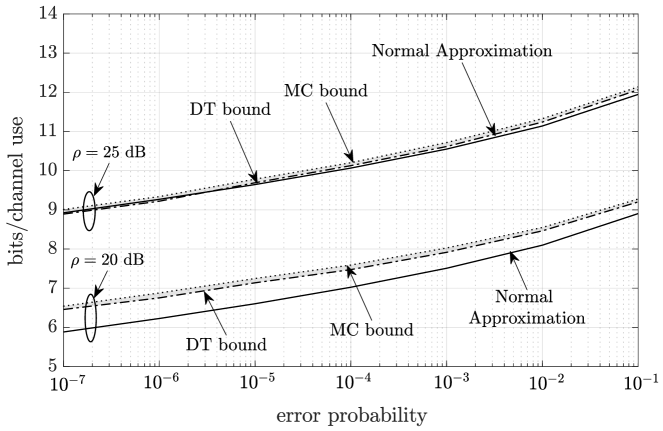
(a) $n_{t}=2$, $n_{r}=2$, $T=24$, and $L=7$.

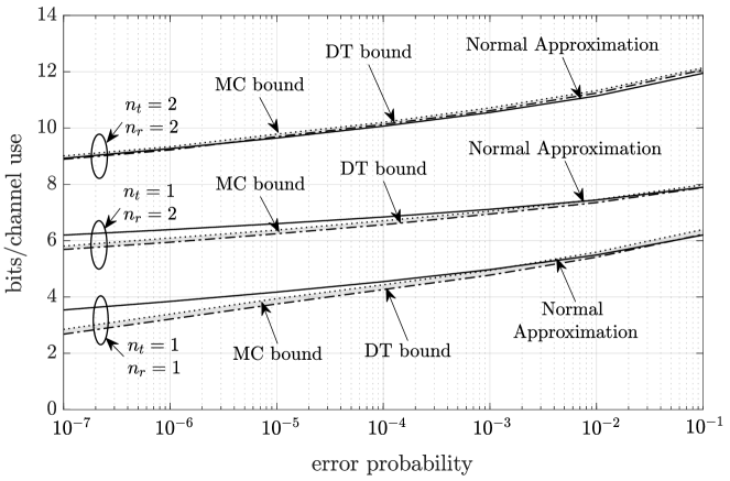
(b) $\rho=25$dB, $T=24$, and $L=7$.

Figure 3: $R^{\ast}(L,T,\epsilon,\rho)$ as a function of $\epsilon$.

In Figs. 3a and 3b, we study $R^{\ast}(L,T,\epsilon,\rho)$ as a function of $\epsilon$ for $T=24$ and $L=7$. Specifically, Fig. 3a plots $R^{\ast}(L,T,\epsilon,\rho)$ for $n_{t}=2,n_{r}=2$, and two different SNR values $20$ dB and $25$ dB. Fig. 3b plots $R^{\ast}(L,T,\epsilon,\rho)$ for $25$ dB and three different numbers of antennas $(n_{t},n_{r})=(1,1)$, $(1,2)$, and $(2,2)$. Observe that the accuracy of normal approximation (6) increases as the SNR value and the number of antennas become larger, and for $\rho=25$ dB and $(n_{t},n_{r})=(2,2)$ it is very close to the non-asymptotic bounds over the entire range of error probabilities considered. For smaller numbers of antennas, the normal approximation loses accuracy at small error probabilities.

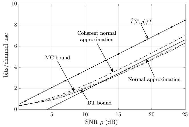
(a) $T=24$, $L=7$, $\epsilon=10^{-5}$, $n_{t}=1$, and $n_{r}=2$.

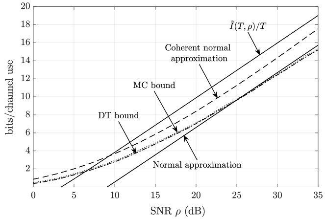
(b) $T=24$, $L=7$, $\epsilon=10^{-5}$, $n_{t}=2$, and $n_{r}=2$.

Figure 4: $R^{\ast}(L,T,\epsilon,\rho)$ as a function of $\rho$.

In Figs. 4a and 4b, we study $R^{\ast}(L,T,\epsilon,\rho)$ as a function of the SNR for $T=24$, $L=7$, $\epsilon=10^{-5}$, and $(n_{t},n_{r})=(1,2)$ and $(2,2)$, respectively. For comparison, we also show the high-SNR approximation $\tilde{I}(T,\rho)$ of channel capacity. First observe that the DT lower bound on $R^{\ast}(L,T,\epsilon,\rho)$ (which is based on USTM channel inputs) is close to the MC upper bound (which is valid for any input distribution satisfying the power constraint (4)). Thus, USTM channel inputs are nearly capacity-achieving for all SNR values considered. Further observe that the SNR range over which the normal approximation (6) is accurate depends on the number of antennas. Specifically, when $n_{t}=1$ and $n_{r}=2$, the normal approximation is accurate for SNR values above $\rho=12$dB, whereas when $n_{t}=2$ and $n_{r}=2$, it is accurate for SNR values above $\rho=23$dB. As expected, the normal approximation of the coherent channel is strictly larger than the high-SNR normal approximation of the non-coherent channel, but its gap to the nonasymptotic bounds decreases as $\rho$ becomes small. Intuitively, this is because, as $\rho$ decreases, knowledge of the fading coefficients becomes less important.

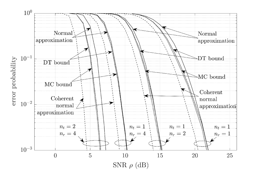
Figure 5: The minimum error probability $\epsilon$ as a function of the SNR for $R=4$, $T=24$, and $L=7$.

In Fig. 5, we plot the error probability as a function of the SNR for a fixed rate $R=4$ and for $T=24$, $L=7$, and the numbers of antennas $(n_{t},n_{r})=(1,1)$, $(1,2)$, $(1,4)$, and $(2,4)$. Note that, the diversity gain grows with the number of antennas, which is reflected in the slopes of the curves. Furthermore, observe that the normal approximation (6) is accurate when the number of transmit antennas is $n_{t}=1$, but it is overly-pessimistic when $n_{t}=2$. In contrast, the coherent normal approximation is overly-optimistic for all parameters considered in this figure. Last but not least, observe that the error probability decreases significantly as the number of antennas increases. This demonstrates the benefit of multiple antennas at the transmitter and receiver at short blocklengths.

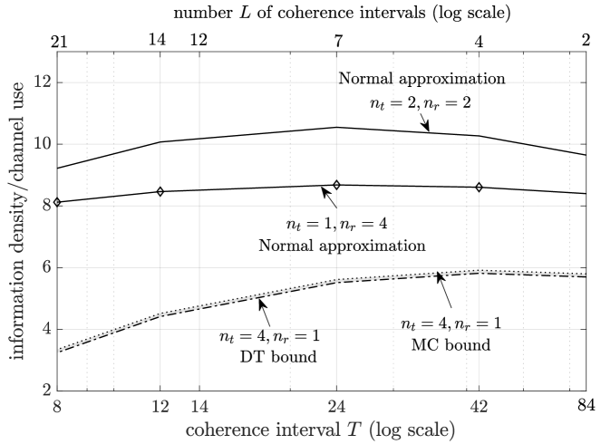
(a) $R^{\ast}(L,T,\epsilon,\rho)$ as a function of $T$ for a fixed $TL=168$, $\epsilon=10^{-3}$, and $\rho=25$ dB.

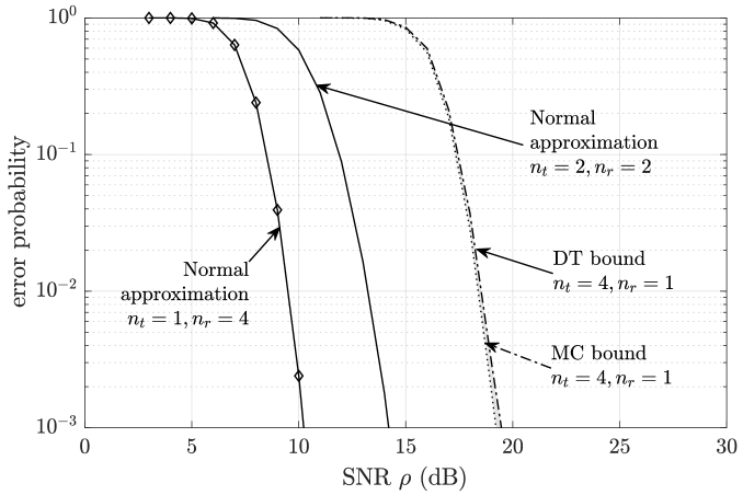
(b) Error probability $\epsilon$ as a function of the SNR for $R=4$, $T=24$, and $L=7$.

Figure 6: Maximum coding rate and minimum error probability for $(n_{t},n_{r})=(1,4)$, $(2,2)$, and $(4,1)$.

Finally, we study the impact of antenna allocation on the maximum coding rate and the error probability when the total number of antennas is equal to $4$. To this end, we plot in Fig. 6a the maximum coding rate $R^{\ast}(L,T,\epsilon,\rho)$ as a function of $T$ for a fixed the blocklength $n=168$ for $\rho=25$ dB, error probability $\epsilon=10^{-3}$, and the numbers of antennas $(n_{t},n_{r})=(1,4)$, $(2,2)$, and $(4,1)$. Similarly, we plot in Fig. 6b the minimum error probability $\epsilon$ as a function of the SNR for $R=4$, $T=24$, $L=7$, and the same numbers of antennas. For the cases $(n_{t},n_{r})=(1,4)$ and $(n_{t},n_{r})=(2,2)$, we plot the normal approximation (6), whereas for the case $(n_{t},n_{r})=(4,1)$ we plot the DT and the MC bound, as the case $n_{t}>n_{r}$ is not covered by Theorem 1. Observe that, for a fixed error probability, the coding rate is maximized by allocating the same number of antennas to the transmitter and receiver. This corresponds to the case where the transmit and receive antennas are used to maximize spatial multiplexing. In contrast, for a fixed rate, the error probability is minimized by maximizing the number of receive antennas. Intuitively, all cases exhibit the same diversity order $n_{t}n_{r}$, but the smallest number of transmit antennas results in the smallest cost for estimating the fading matrix $\mathbf{H}_{\ell}$. For example, estimating $\mathbf{H}_{\ell}$ by means of pilot symbols would require one pilot symbol per coherence interval and transmit antenna. This agrees with the observation made in [28] that, at high SNR, using more transmit than receive antennas does not increase channel capacity.

III-C Engineering Wisdom

III-C1 Optimal number of active transmit antennas

In [28], Zheng and Tse showed that, at high SNR, the channel capacity of the noncoherent Rayleigh block-fading channel behaves as

$$C(\rho)=n_{t_{\star}}\left(1-\frac{n_{t_{\star}}}{T}\right)\log(\rho)+\mathcal{O}_{\rho}(1)$$ (16)

where $n_{t_{\star}}=\min\{n_{t},n_{r},\lfloor T/2\rfloor\}$ corresponds to the number of active transmit antennas out of $n_{t}$ available transmit antennas. If $T\geq n_{t}+n_{r}$ and $n_{t}\leq n_{r}$, then $n_{t_{\star}}=n_{t}$ and the pre-log factor $n_{t}(1-n_{t}/T)$ is monotonically increasing in $n_{t}$. In this case, it is optimal to use all available transmit antennas. However, it is prima facie unclear whether the same is true at finite blocklength. Intuitively, increasing the number of transmit antennas achieves a higher multiplexing gain $\min\{n_{t},n_{r}\}$, but it also requires the estimation of more channel coefficients. To gain some insights on this question, we analyze the behavior of the high-SNR normal approximation (6) as a function of the number of transmit antennas $n_{t}$ for a given number of receive antennas $n_{r}$.

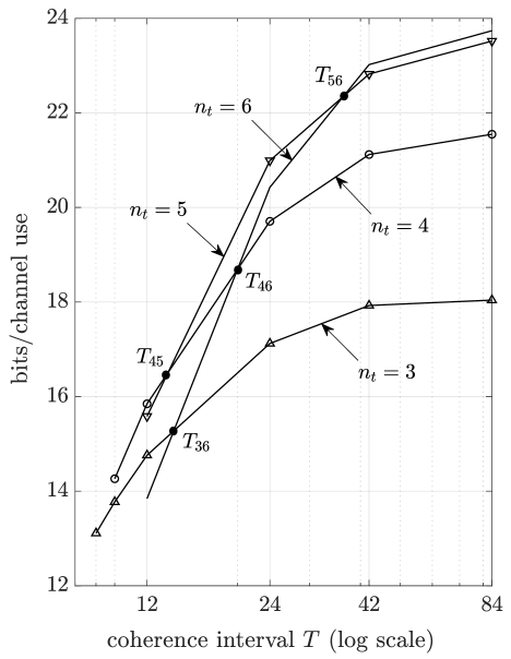
(a) $n=168$, $\epsilon=10^{-3}$, $\rho=20$ dB, and $n_{r}=6$. The crossing points are $T_{36}=13$, $T_{45}=13$, $T_{46}=18$, and $T_{56}=35$.

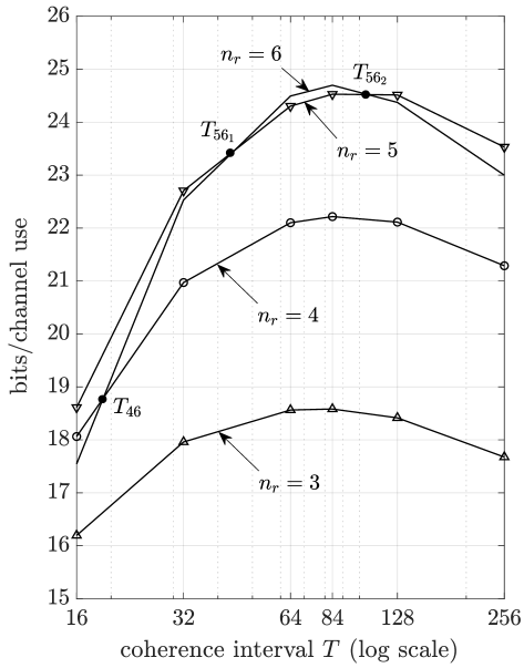
(b) $n=512$, $\epsilon=10^{-5}$, $\rho=20$ dB, and $n_{r}=6$. The crossing points are $T_{46}=18$, $T_{56_{1}}=45$, and $T_{56_{2}}=116$.

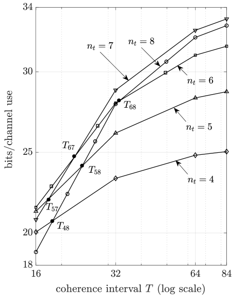
(c) $n=512$, $\epsilon=10^{-5}$, $\rho=20$ dB, and $n_{r}=8$. The crossing points are $T_{48}=18$, $T_{57}=18$, $T_{58}=23$, $T_{67}=22$, and $T_{68}=33$.

Figure 7: High-SNR normal approximation (6) as a function of $T$ for a fixed $n=TL$, a given number of receive antennas, and varying numbers of transmit antennas.

In Fig. 7, we plot the high-SNR normal approximation (6) as a function of $T$ for a fixed blocklength $n=LT$, a given number of receive antennas, and varying numbers of transmit antennas. We set $\rho=20$ dB and consider the cases $(\epsilon=10^{-3},n=168,n_{r}=6)$ (Fig. 7a), $(\epsilon=10^{-5},n=512,n_{r}=6)$ (Fig. 7b), and $(\epsilon=10^{-5},n=512,n_{r}=8)$ (Fig. 7c). We further indicate the values of the coherence interval where two lines cross. Specifically, we use the notation $T_{n_{1}n_{2}}$ to indicate the crossing point of the curves for $n_{t}=n_{1}$ and $n_{t}=n_{2}$. Observe that, in contrast to the pre-log factor of the high-SNR asymptotic capacity, the number of transmit antennas that maximizes the high-SNR normal approximation is not necessarily equal to the maximum value $n_{t}=n_{r}$ and depends on the coherence interval $T$. For example, according to Fig. 7a, when $n=168$ and $n_{r}=6$, the maximum number of available transmit antennas should only be used when $T\geq 35$. Furthermore, when $n=512$ and $n_{r}=8$, using all available transmit antennas is actually suboptimal over the entire range of $T$; cf. Fig. 7c. Instead, it is optimal to only use $7$ transmit antennas. Finally, the optimal number of active transmit antennas is not necessarily monotonically increasing in $T$. As can be observed from Fig. 7b, when $n=512$ and $n_{r}=6$, using all available transmit antennas is only optimal when $45\leq T\leq 116$.

In summary, while the high-SNR asymptotic capacity (16) suggest that, at large blocklengths and high SNR, it is optimal to use all available transmit antennas, in general the maximum coding rate has a more intricate dependence on the number of active transmit antennas. The high-SNR normal approximation presented in Theorem 1 allows us to unveil this dependence without the need to resorting to nonasymptotic bounds that need to be evaluated numerically at a high computation cost.

III-C2 Normal approximation applied in slotted-ALOHA protocol

As argued, e.g., in [1], the normal approximation can be used to analyze the performance of communication protocols; see, e.g.  [6, 7, 8, 9, 10, 11, 12, 13, 14, 15]. To illustrate this, we shall to analyze the probability of successful transmission in the slotted-ALOHA protocol, where $\mathsf{d}$ devices intend to send $\mathsf{k}$ information bits to a base station within the time corresponding to $n$ channel uses. The $n$ channel uses are divided into $\mathsf{s}$ equally-sized slots of $n_{\mathsf{s}}=n/\mathsf{s}$ channels uses and the devices apply a simple slotted-ALOHA protocol: each device picks randomly one of the $\mathsf{s}$ slots in the frame and sends its packet. A collision occurs if two or more devices pick the same slot. The normal approximation can be used to calculated the error probability if there is no collision.

For example, the normal approximation for the multi-antenna AWGN channel with $n_{t}$ transmit and $n_{r}$ receive antennas and a spatial multiplex gain $n_{\textnormal{min}}\triangleq\min(n_{t},n_{r})$ is given by [34, Th. 78]

$$R^{\ast}(n,\epsilon)\approx C_{\textnormal{P-AWGN}}(\rho)-\sqrt{\frac{V_{\textnormal{P-AWGN}}(\rho)}{n}}Q^{-1}(\epsilon)+\frac{1}{2}\frac{\log n}{n}$$ (17)

where

$$C_{\textnormal{P-AWGN}}(\rho) = n_{\textnormal{min}}\log\left(1+\frac{\rho}{n_{\textnormal{min}}}\right)$$

$$V_{\textnormal{P-AWGN}}(\rho) = \rho\frac{2+\frac{\rho}{n_{\textnormal{min}}}}{(1+\frac{\rho}{n_{\textnormal{min}})^{2}}}.$$

By solving (17) for $\epsilon$, we obtain an approximation of the packet error probability as a function of the packet length $n$, the number of information bits $\mathsf{k}=nR$ to be conveyed in a packet, and the SNR $\rho$:

$$\epsilon^{\ast}(\mathsf{k},n,\rho)\approx Q\left(\frac{nC_{\textnormal{P-AWGN}}(\rho)-\mathsf{k}\log 2+\log n/2}{\sqrt{nV_{\textnormal{P-AWGN}}(\rho)}}\right).$$ (18)

Replacing (17) by the normal approximation for the coherent Rayleigh block-fading channel [18], we obtain the approximation

$$\epsilon^{\ast}(\mathsf{k},n,\rho)\approx Q\left(\frac{nC_{c}(\rho)-\mathsf{k}\log 2}{\sqrt{nV_{c}(T,\rho)}}\right)$$ (19)

where

$$C_{c}(\rho) = \sum_{i=1}^{n_{\textnormal{min}}}\mathbb{E}\left[\log\left(1+\frac{\rho}{n_{t}}\Lambda_{i}^{2}\right)\right]$$

$$V_{c}(T,\rho) = T\text{Var}\left(\sum_{i=1}^{n_{\textnormal{min}}}\log\left(1+\frac{\rho}{n_{t}}\Lambda_{i}^{2}\right)\right)+\sum_{i=1}^{n_{\textnormal{min}}}\mathbb{E}\left[1-\frac{1}{\left(1+\frac{\rho}{n_{t}}\Lambda_{i}^{2}\right)^{2}}\right]+\left(\frac{\rho}{n_{t}}\right)^{2}\left(\eta_{1}-\frac{\eta_{2}}{n_{t}}\right),$$

$\Lambda_{i}^{2}$, $i=1,\ldots,n_{\textnormal{min}}$ are the eigenvalues of $\mathbf{H}_{\ell}\mathbf{H}_{\ell}^{\mathsf{H}}$, and

$$\eta_{1} \triangleq \sum_{i=1}^{n_{\textnormal{min}}}\mathbb{E}\left[c^{2}(\Lambda_{i}^{2})\right]$$

$$\eta_{2} \triangleq \left(\sum_{i=1}^{n_{\textnormal{min}}}\mathbb{E}\left[c(\Lambda_{i}^{2})\right]\right)^{2}$$

$$c(x) \triangleq \frac{x}{1+\frac{\rho}{n_{t}}x}.$$

Likewise, replacing (17) by our high-SNR normal approximation for the noncoherent Rayleigh block-fading channel, we obtain the approximation

$$\epsilon^{\ast}(\mathsf{k},n,\rho)\approx Q\left(\frac{n\tilde{I}(T,\rho)-\mathsf{k}T\log 2}{\sqrt{nT\tilde{V}(T)}}\right).$$ (20)

The probability of successful transmission is given by [1, Eq. (24)]

$$P_{s}=\frac{\mathsf{d}}{\mathsf{s}}\left(1-\frac{1}{\mathsf{s}}\right)^{\mathsf{d}-1}\Big{(}1-\epsilon^{\ast}(\mathsf{k},n_{\mathsf{s}},\rho)\Big{)}$$

By utilizing the normal approximations (18), (19), and (20), we can study fundamental tradeoffs between the number of slots $\mathsf{s}$, the probability of successful transmission, and the number of information bits $\mathsf{k}$ for a given number of devices $\mathsf{d}$, blocklength $n$, SNR $\rho$, and number of antennas $(n_{t},n_{r})$. For example, the optimization of the number of slots entails a tradeoff between the probability of collision and the number of channel uses available for each packet, which affects the achievable error probability in a singleton slot. Indeed, if $\mathsf{s}$ increases, then the probability of a collision decreases, but the packet error probability for a singleton slot increases. Conversely, if $\mathsf{s}$ decreases, then the packet error probability for a singleton slot decreases, but the probability of a collision increases.

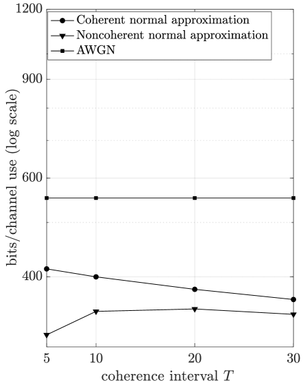
(a) $n_{t}=1,n_{r}=1$.

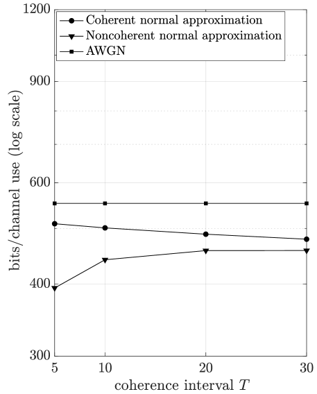
(b) $n_{t}=1,n_{r}=2$.

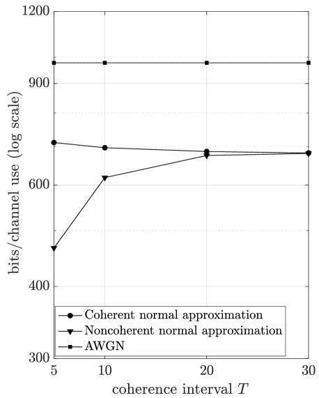
(c) $n_{t}=2,n_{r}=2$.

Figure 8: Maximum number of bits $\mathsf{k}$ that can be transmitted successfully with probability $P_{s}\geq 0.3$ for $n=TL=480$, $\mathsf{d}=12$, and $\rho=25$ dB.

For $\mathsf{d}=12$ devices, the maximum probability of successful transmission $P_{s}$ is equal to $0.384$ and is achieved for $\mathsf{s}=\mathsf{d}=12$ and $\epsilon^{\ast}(\mathsf{k},n_{\mathsf{s}},\rho)=0$. However, a vanishing error probability for a singleton slot would require that either the blocklength $n_{\mathsf{s}}$ or the SNR $\rho$ tend to infinity. Consequently, for short-package communications, the probability of successful transmission is strictly smaller than $0.384$. In Fig. 8, we depict the maximum number of information bits $\mathsf{k}$ that can be transmitted successfully with probability $P_{s}\geq 0.3$ when $n=480$, $\mathsf{d}=12$, and $\rho=25$ dB. The three subplots correspond to the numbers of antennas $(n_{t},n_{r})=(1,1)$, $(1,2)$, and $(2,2)$. An exhaustive search over $\mathsf{s}$ and $\mathsf{k}$ shows that, for the AWGN channel, the optimal error probability for a singleton slot is $\epsilon^{\ast}(\mathsf{k},n_{\mathsf{s}},\rho)\approx 0.0462$ and the optimal number of slots is $\mathsf{s}=7$, whereas for the Rayleigh block-fading channel (both coherent and noncoherent), the optimal error probability for a singleton slot is $\epsilon^{\ast}(\mathsf{k},n_{\mathsf{s}},\rho)\approx 0.1312$ and the optimal number of slots is $\mathsf{s}=8$.

Observe that the AWGN channel achieves the largest transmission bits $\mathsf{k}$. Furthermore, the gap between the noncoherent and the coherent case becomes smaller as $T$ increases, which agrees with the intuition that the cost for estimating the channel reduces as $T$ increases. Finally, the maximum number of bits $\mathsf{k}$ that can be transmitted successfully benefits more from an increase in the coherence interval $T$ if the number of antennas is larger. Intuitively, a larger number of antennas may yield more diversity and multiplexing gain, provided that we have a sufficiently accurate estimate of the fading coefficients.

IV Proof of Theorem 1

To prove Theorem 1, we derive in Section IV-A a lower bound on $R^{*}(L,T,\epsilon,\rho)$ and in Section IV-B an upper bound on $R^{*}(L,T,\epsilon,\rho)$. Since both bounds are equal to (6) up to error terms that have the same behaviors as $K_{\tilde{I}}(T,\rho)$, $K_{\tilde{V}}(T,\rho)$, and $K_{L}(L,T,\rho)$ (cf. (34) and (89)), we conclude that $R^{*}(L,T,\epsilon,\rho)$ is given by (6).

IV-A Dependence Testing Lower Bound

To derive a lower bound on $R^{\ast}(L,T,\epsilon,\rho)$, we evaluate the DT lower bound [3, Th. 22] for an USTM input distribution. Such an input can be written as $\mathbf{X}^{L}=\sqrt{T\rho/n_{t}}\mathbf{U}^{L}$, where $\mathbf{U}^{L}=[\mathbf{U}_{1},\ldots,\mathbf{U}_{L}]$ is a sequence of i.i.d., isotropically distributed, random matrices satisfying $\mathbf{U}_{\ell}^{\mathsf{H}}\mathbf{U}_{\ell}=\mathsf{I}_{n_{t}}$, $\ell=1,\ldots,L$. We define the information density between the random vectors $\mathbf{X}^{L}$ and $\mathbf{Y}^{L}$ as

$$i(\mathbf{X}^{L};\mathbf{Y}^{L})\triangleq\log\left(\frac{f_{\mathbf{Y}^{L}|\mathbf{X}^{L}}(\mathbf{Y}^{L}|\mathbf{X}^{L})}{f_{\mathbf{Y}^{L}}(\mathbf{Y}^{L})}\right)$$

where $f_{\mathbf{Y}^{L}|\mathbf{X}^{L}}$ denotes the conditional probability density function (pdf) of the channel outputs $\mathbf{Y}^{L}$ of the channel (3) given the channel inputs $\mathbf{X}^{L}$ and $f_{\mathbf{Y}^{L}}$ is the output pdf induced by the input distribution and the channel law. When the input distribution is USTM, the channel outputs $\mathbf{Y}^{L}=[\mathbf{Y}_{1},\ldots,\mathbf{Y}_{L}]$ are i.i.d., $(T\times n_{r})$-dimensional random matrices whose joint pdf is given by

$$f_{\mathbf{Y}^{L}}(\mathsf{Y}^{L})=\prod_{\ell=1}^{L}f_{\mathbf{Y}}^{(U)}(\mathsf{Y}_{\ell}),\quad\mathsf{Y}^{L}=[\mathsf{Y}_{1},\ldots,\mathsf{Y}_{L}]$$ (21)

where $f_{\mathbf{Y}}^{(U)}$ denotes the pdf of the outputs of the channel (3) in each coherence interval induced by USTM channel inputs. Since the channel is blockwise memoryless, the information density can be expressed as

$$i(\mathbf{X}^{L};\mathbf{Y}^{L})=\sum_{\ell=1}^{L}i_{\ell}(T,\rho)$$

where

$$i_{\ell}(T,\rho)\triangleq\log\frac{f_{\mathbf{Y}|\mathbf{X}}(\mathbf{Y}_{\ell}|\mathbf{X}_{\ell})}{f_{\mathbf{Y}}^{(U)}(\mathbf{Y}_{\ell})}$$

and $f_{\mathbf{Y}|\mathbf{X}}$ denotes the conditional pdf of the channel output $\mathbf{Y}_{\ell}$ in coherence interval $\ell$ given the corresponding channel input $\mathbf{X}_{\ell}$.

To apply the DT bound, we first note that the cumulative distribution function $\Pr\big{[}i(\mathbf{x}^{L};\tilde{\mathbf{Y}}^{L})\leq\alpha\big{]}$ for $\mathbf{Y}^{L}$ distributed according to (21) does not depend on $\mathbf{x}^{L}$. Furthermore, the UMTS input distribution satisfies the power constraint (4) with probability one. After a standard change of measure, it thus follows from [3, Ths. 22 & 23] that there exists a code of blocklength $n=LT$ with $M$ codewords whose maximum error probability satisfies

$$\epsilon\leq(M-1)\mathsf{E}\left[e^{-i(\mathbf{X}^{L};\mathbf{Y}^{L})}\mathds{1}\left\{i(\mathbf{X}^{L};\mathbf{Y}^{L})>\log(M-1)\right\}\right]+\Pr\left[i(\mathbf{X}^{L};\mathbf{Y}^{L})\leq\log(M-1)\right].$$ (22)

Consequently, if we can find an $M$ such that the right-hand side (RHS) of (22) is upper-bounded by $\epsilon$, then there exists an $(L,T,M,\epsilon,\rho)$ code with these parameters. By the definition of the maximum coding rate (5), we then obtain the lower bound

$$R^{*}(L,T,\epsilon,\rho)\geq\frac{\log M}{LT}.$$

To find such an $M$, we shall closely follow [3, Eqs. (258)–(267)] (see also [27, Eqs. (69)–(85)]). To this end, we will need the following auxiliary results. In the following, and throughout the paper, we shall omit the subscript $\ell$ where it is immaterial.

Lemma 1

Let $I(T,\rho)\triangleq\mathsf{E}[i(T,\rho)]$ and $\underline{U}(T,\rho)\triangleq\mathsf{E}\bigl{[}\bigl{(}i(T,\rho)-I(T,\rho)\bigl{)}^{2}\bigl{]}$. At high SNR, $\underline{U}(T,\rho)$ can be approximated as

$$\underline{U}(T,\rho)=T^{2}\tilde{V}(T)+K_{\underline{U}}(T,\rho)$$

where $\tilde{V}(T)$ is defined in (8) and $K_{\underline{U}}(T,\rho)$ is a function of $T$ and $\rho$ that satisfies

$$\lim\limits_{\rho\to\infty}K_{\underline{U}}(T,\rho)=0.$$

Proof:

See Appendix A. ∎

Lemma 2

There exists a sufficiently large $\rho_{0}$ (that only depends on $T$) such that

$$\sup_{\rho\geq\rho_{0}}\underline{U}(T,\rho) <\infty$$

$$\sup_{\rho\geq\rho_{0}}\mathsf{E}\big{[}\big{|}i(T,\rho)-I(T,\rho)\big{|}^{3}\big{]} <\infty.$$

Proof:

See Appendix B. ∎

Lemma 1 implies that there exists a sufficiently large $\rho_{0}$ (that only depends on $T$) such that

$$\underline{U}(T,\rho)\geq\frac{\tilde{V}(T)}{2},\quad\rho\geq\rho_{0}.$$ (23)

Furthermore, by Lemma 2, there exist a sufficiently large $\rho_{0}$ and an $\underline{S}(T,\rho_{0})$ that is independent of $\rho$ such that

$$\mathsf{E}\big{[}\big{|}i(T,\rho)-I(T,\rho)\big{|}^{3}\big{]}\leq\underline{S}(T,\rho_{0}),\qquad\rho\geq\rho_{0}.$$ (24)

Combining (23) and (24), it then follows that

$$\frac{6\mathsf{E}\big{[}\big{|}i(T,\rho)-I(T,\rho)\big{|}^{3}\big{]}}{\underline{U}(T,\rho)^{3/2}}\leq\frac{6\underline{S}(T,\rho_{0})}{\left[\frac{\tilde{V}(T)}{2}\right]^{3/2}}\triangleq\underline{B}(T,\rho_{0}),\quad\rho\geq\rho_{0}.$$ (25)

We next use (25) together with the Berry-Esseen theorem [35, Ch. XVI.5] to upper-bound the second term on the RHS of (22). Indeed, let

$$\tau=Q^{-1}\left(\epsilon-\left(\frac{2\log 2}{\sqrt{2\pi}}+5\underline{B}(T,\rho_{0})\right)\frac{1}{\sqrt{L}}\right)$$

and set

$$\log(M-1)=LI(T,\rho)-\tau\sqrt{L\underline{U}(T,\rho)}.$$ (26)

Then,

$$\Pr\left[i(\mathbf{X}^{L};\mathbf{Y}^{L})\leq\log(M-1)\right] \leq Q(-\tau)+\frac{6\mathsf{E}\big{[}\big{|}i(T,\rho)-I(T,\rho)\big{|}^{3}\big{]}}{\sqrt{L}\big{(}\underline{U}(T,\rho)\big{)}^{3/2}}$$ (27)

$$\leq \epsilon-\left(\frac{2\log 2}{\sqrt{2\pi}}+5\underline{B}(T,\rho_{0})\right)\frac{1}{\sqrt{L}}+\frac{\underline{B}(T,\rho_{0})}{\sqrt{L}}$$

$$= \epsilon-2\left(\frac{\log 2}{\sqrt{2\pi}}+2\underline{B}(T,\rho_{0})\right)\frac{1}{\sqrt{L}}$$

where the first step follows from the Berry-Esseen theorem and the second step follows from (25) and the definition of $\tau$. The first term on the RHS of (22) can be upper-bounded using [3, Lemma 47] as

$$(M-1)\mathsf{E}\left[e^{-i(\mathbf{X}^{L};\mathbf{Y}^{L})}\mathds{1}\left\{i(\mathbf{X}^{L};\mathbf{Y}^{L})>\log(M-1)\right\}\right]\leq 2\left(\frac{\log 2}{\sqrt{2\pi}}+2\underline{B}(T,\rho_{0})\right)\frac{1}{\sqrt{L}}.$$ (28)

It can be checked that the sum of the RHSs of (27) and (28) is equal to $\epsilon$. Consequently, there exists an $(L,T,M,\epsilon,\rho)$ code with $M$ given in (26) and we have

$$R^{\ast}(L,T,\epsilon,\rho) \geq \frac{\log(M-1)}{LT}$$ (29)

$$= \frac{I(T,\rho)}{T}-\sqrt{\frac{\underline{U}(T,\rho)}{LT^{2}}}Q^{-1}\left(\epsilon-\left(\frac{2\log 2}{\sqrt{2\pi}}+5\underline{B}(T,\rho_{0})\right)\frac{1}{\sqrt{L}}\right).$$

A Taylor-series expansion of $Q^{-1}(\cdot)$ around $\epsilon$ yields that

$$\left|Q^{-1}\left(\epsilon-\left(\frac{2\log 2}{\sqrt{2\pi}}+5\underline{B}(T,\rho_{0})\right)\frac{1}{\sqrt{L}}\right)-Q^{-1}(\epsilon)\right|\leq\frac{A}{\sqrt{L}},\quad L\geq L_{0}$$ (30)

for some constants $A$, and $L_{0}$ that are independent of $L$ and $\rho$. Furthermore, Lemma 2 shows that $\underline{U}(T,\rho)$ is uniformly bounded in $\rho\geq\rho_{0}$. Thus, combining (29) and (30), we obtain

$$R^{\ast}(L,T,\epsilon,\rho)\geq\frac{I(T,\rho)}{T}-\sqrt{\frac{\underline{U}(T,\rho)}{LT^{2}}}Q^{-1}(\epsilon)+K_{\textnormal{DT}}(L,T,\rho)$$ (31)

where $K_{\textnormal{DT}}(L,T,\rho)$ is a function of $L$, $T$, and $\rho$ that satisfies

$$\sup_{\rho\geq\rho_{0}}\big{|}K_{\textnormal{DT}}(L,T,\rho)\big{|}\leq\frac{A}{L},\quad L\geq L_{0}$$

for some constants $A$, $L_{0}$, and $\rho_{0}$ that are independent of $L$ and $\rho$.

At high SNR, $I(T,\rho)/T$ and $\underline{U}(T,\rho)/T^{2}$ can be approximated as

$$\frac{I(T,\rho)}{T} = \tilde{I}(T,\rho)+\tilde{K}_{{I}}(T,\rho)$$ (32)

$$\frac{\underline{U}(T,\rho)}{T^{2}} = \tilde{V}(T)+\tilde{K}_{\underline{U}}(T,\rho)$$ (33)

where $\tilde{I}(T,\rho)$ and $\tilde{V}(T)$ are given in (7) and (8), and where $\tilde{K}_{\xi}(T,\rho)$, $\xi\in\{{I},\underline{U}\}$ are functions of $T$ and $\rho$ that both satisfy $\lim\limits_{\rho\to\infty}K_{\xi}(T,\rho)=0$. Here, (32) follows from [29, Eq. (49)] and (33) follows from Lemma 1. Combining (32) and (33) with (31), we obtain that

$$R^{\ast}(L,T,\epsilon,\rho)\geq\tilde{I}(T,\rho)+\tilde{K}_{{I}}(T,\rho)-\sqrt{\frac{\tilde{V}(T)+\tilde{K}_{\underline{U}}(T,\rho)}{L}}Q^{-1}(\epsilon)+K_{\textnormal{DT}}(L,T,\rho)$$ (34)

Note that $\tilde{K}_{\xi}(T,\rho)$, $\xi\in\{I,\underline{U}\}$ satisfy (9) and $K_{\textnormal{DT}}(L,T,\rho)$ satisfies (10).

IV-B Meta Converse Upper Bound

Our upper bound on $R^{\ast}(L,T,\epsilon,\rho)$ is based on the MC bound [3, Th. 31], which states that the cardinality of a codebook $\mathcal{C}$ with codewords $(\mathsf{X}_{1},\ldots,\mathsf{X}_{L})$ belonging to the set $\mathcal{F}$ and maximum error probability not exceeding $\epsilon$ satisfies

$$\log|\mathcal{C}|\leq\sup_{\mathsf{X}^{L}\in\mathcal{F}}\log\frac{1}{\beta_{1-\epsilon}(\mathsf{X}^{L},q_{\mathbf{Y}^{L}})}$$ (35)

where $\beta_{1-\epsilon}(\mathsf{X}^{L},q_{\mathbf{Y}^{L}})$ denotes the minimum probability of error of a binary hypothesis test under hypothesis $q_{\mathbf{Y}^{L}}$ if the probability of error under hypothesis $f_{\mathbf{Y}^{L}|\mathbf{X}^{L}}$ does not exceed $\epsilon$ [3, Eq. (100)], and $q_{\mathbf{Y}^{L}}$ is an auxiliary pdf on the output alphabet. In this paper, we choose the auxiliary pdf that was chosen in [29, Sec. IV-A] to derive an upper bound on the channel capacity of non-coherent MIMO Rayleigh block-fading channels, namely, $q_{\mathbf{Y}^{L}}=q_{\mathbf{Y}}\times\ldots\times q_{\mathbf{Y}}$ is a product distribution with

$$q_{\mathbf{Y}}(\mathsf{Y})=\frac{1}{\mu^{n_{t}n_{r}}\pi^{n_{r}T}}\frac{\Gamma_{n_{t}}(T)}{\Gamma_{n_{t}}(n_{t})}e^{-\sum_{i=1}^{n_{t}}\frac{\sigma_{i}^{2}}{\mu}}e^{-\sum_{i=n_{t}+1}^{n_{r}}\sigma_{i}^{2}}\frac{1}{\big{(}\prod_{i=1}^{n_{t}}\sigma_{i}^{2}\big{)}^{T-2n_{r}+n_{t}}}\frac{1}{\prod_{i=1}^{n_{t}}\prod_{j=n_{t}+1}^{n_{r}}(\sigma_{i}^{2}-\sigma_{j}^{2})^{2}}$$ (36)

where $\sigma_{1}\geq\ldots\geq\sigma_{n_{r}}$ are the ordered nonzero singular values of $\mathsf{Y}$ and $\mu\triangleq T\rho/n_{t}$.

We next note that, for every $T\times T$ unitary matrix $\mathsf{A}$ and every $\mathsf{X}$ and $\mathsf{Y}$, [24, Eqs. (54) & (55)]

$$f_{\mathbf{Y}|\mathbf{X}}(\mathsf{Y}_{\ell}|\mathsf{A}\mathsf{X}_{\ell}) = f_{\mathbf{Y}|\mathbf{X}}(\mathsf{A}\mathsf{Y}_{\ell}|\mathsf{X}_{\ell})$$

$$q_{\mathbf{Y}}(\mathsf{A}\mathsf{Y}) = q_{\mathbf{Y}}(\mathsf{Y}).$$

It then follows from [36, Prop. 19] that $\beta_{1-\epsilon}(\mathsf{X}^{L},q_{\mathbf{Y}^{L}})$ does not change if we multiply the channel input $\mathsf{X}_{\ell}$ by a unitary matrix $\mathsf{A}_{\ell}$. We further note that

$$f_{\mathbf{Y}|\mathbf{X}}(\mathsf{Y}_{\ell}|\mathsf{X}_{\ell})=\frac{e^{-\text{tr}\left(\mathsf{Y}_{\ell}^{\mathsf{H}}(\mathsf{I}_{T}+\rho T/n_{t}\mathsf{X}_{\ell}\mathsf{X}_{\ell}^{\mathsf{H}})^{-1}\mathsf{Y}_{\ell}\right)}}{\pi^{n_{r}T}(1+\rho T/n_{t})^{n_{t}n_{r}}}$$

and, hence, also $\beta_{1-\epsilon}(\mathsf{X}^{L},q_{\mathbf{Y}^{L}})$ depends on $\mathsf{X}_{\ell}$ only via the product $\mathsf{X}_{\ell}\mathsf{X}_{\ell}^{\mathsf{H}}$. By expressing $\mathsf{X}_{\ell}$ in terms of its singular value decomposition

$$\mathsf{X}_{\ell}=\mathsf{U}_{\ell}\Sigma_{\ell}\mathsf{V}_{\ell}^{\mathsf{H}}$$

and by setting $\mathsf{A}_{\ell}=\mathsf{U}_{\ell}^{\mathsf{H}}$, we thus obtain that we can restrict ourselves without loss of optimality to channel inputs $\mathsf{X}_{\ell}$ that are given by a $T\times n_{t}$ rectangular diagonal matrix with diagonal entries $d_{1,\ell},\ldots,d_{n_{t},\ell}$. Intuitively, $d_{i,\ell}^{2}$ denotes the power at transmit antenna $i=1,\ldots,n_{t}$ and coherence interval $\ell=1,\ldots,L$. Let $\mathsf{D}_{\ell}\triangleq\text{diag}\bigl{\{}d_{1,\ell},\ldots,d_{n_{t},\ell}\bigr{\}}$ and $\alpha_{\ell}\triangleq\text{tr}(\mathsf{D}_{\ell}^{2})/T$. Thus, $\mathsf{D}_{\ell}$ is the diagonal square matrix that is composed of the first $n_{t}$ columns and rows of $\mathsf{X}_{\ell}$, i.e., $\mathsf{D}_{\ell}=[\mathsf{X}_{\ell}]_{(1:n_{t})^{2}}$. By the power constraint (4), we have for every $\ell$ that $0\leq\alpha_{\ell}\leq\rho$.

To derive an upper bound on $R^{*}(L,T,\epsilon,\rho)$, we follow the idea in [19] and separate the codebook $\mathcal{C}$ into two sub-codebooks $\mathcal{C}_{1}$ and $\mathcal{C}_{2}$. Clearly, if the maximum error probabilities of $\mathcal{C}_{1}$ and $\mathcal{C}_{2}$ are $\epsilon$, then the maximum error probability of $\mathcal{C}$ cannot be smaller than $\epsilon$. Specifically, $\mathcal{C}_{1}$ contains all the codewords for which $d_{i,\ell}^{2}>\bar{\delta}\rho$, $i=1,\cdots,n_{t}$ (with $\bar{\delta}$ defined in (38)) in at least half of the coherence intervals. The second codebook $\mathcal{C}_{2}$ contains the remaining codewords. We then upper-bound the cardinalities of both codewords using a weakened version of the MC bound (35), namely, [3, Th. 31 & Eq. (102)]

$$\log|\mathcal{C}_{i}|\leq\sup_{\mathsf{X}^{L}\in\mathcal{C}_{i}}\bigg{\{}\log\xi(\mathsf{D}^{L})-\log\bigg{(}1-\epsilon-\Pr\biggl{[}j(\mathbf{X}^{L};\mathbf{Y}^{L})\geq\log\xi(\mathsf{D}^{L})\biggm{|}\mathbf{X}^{L}=\mathsf{X}^{L}\biggr{]}\bigg{)}\bigg{\}},\quad i=1,2$$ (37)

for an arbitrary threshold $\xi(\mathsf{D}^{L})$ which may depend on $\mathsf{D}^{L}$ and which we shall define later. Here,

$$j(\mathbf{X}^{L};\mathbf{Y}^{L})\triangleq\sum_{\ell=1}^{L}\log\left(\frac{f_{\mathbf{Y}|\mathbf{X}}(\mathbf{Y}_{\ell}|\mathbf{X}_{\ell})}{q_{\mathbf{Y}}(\mathbf{Y}_{\ell})}\right)$$

is the so-called mismatched information density. We conclude by showing that, when both $\rho$ and $L$ tend to infinity, the cardinality of the entire codebook $\mathcal{C}$ can be approximated by the cardinality of $\mathcal{C}_{1}$. Consequently, $R^{\ast}(L,T,\epsilon,\rho)$ is asymptotically upper-bounded by the upper bound on the maximum coding rate of $\mathcal{C}_{1}$.

To define $\mathcal{C}_{1}$ and $\mathcal{C}_{2}$ mathematically, we first introduce the sets

$$\mathcal{D}_{1} \triangleq \big{\{}\mathsf{D}\in\mathcal{D}_{n_{t}}:d_{i}^{2}>\bar{\delta}\rho,~i=1,\ldots,n_{t}\big{\}},$$

$$\mathcal{D}_{2} \triangleq \mathcal{D}_{n_{t}}\setminus\mathcal{D}_{1},$$

where $\mathcal{D}_{n_{t}}$ denotes the set of $(n_{t}\times n_{t})$-dimensional diagonal matrices $\mathsf{D}$ with non-negative, real-valued entries that satisfy $\text{tr}(\mathsf{D}^{2})\leq T\rho$; and $d_{i}$ denotes the $i$-th diagonal element of $\mathsf{D}$. Further let

$$\bar{\delta}\triangleq\frac{T}{n_{t}}-\frac{T}{2n_{r}\sqrt{n_{t}}\sqrt{\mathsf{E}\big{[}\log\det(\mathbf{H}_{\ell}\mathbf{H}_{\ell}^{\mathsf{H}})^{2}\big{]}}+1}.$$ (38)

By using that, by [31, Lemmas A.1 & A.2],

$$\mathsf{E}\big{[}\log\det(\mathbf{H}_{\ell}\mathbf{H}_{\ell}^{\mathsf{H}})^{2}\big{]}=\mathsf{E}\big{[}\log\det(\mathbf{H}_{\ell}\mathbf{H}_{\ell}^{\mathsf{H}})\big{]}^{2}+\mathrm{Var}\big{(}\log\det(\mathbf{H}_{\ell}\mathbf{H}_{\ell}^{\mathsf{H}})\big{)}=\sum_{i=0}^{n_{t}-1}\varPsi(n_{t}-i)+\sum_{i=0}^{n_{t}-1}\varPsi^{\prime}(n_{t}-i)$$ (39)

and that $n_{t}\leq n_{r}$ (by assumption) and $\varPsi^{\prime}(1)=\pi^{2}/6$ [37, Th. 2.11], it can be shown that $\bar{\delta}>0$.

For a sequence of matrices $\mathsf{D}^{L}=(\mathsf{D}_{1},\ldots,\mathsf{D}_{L})$, let

$$L_{\mathcal{D}_{1}}(\mathsf{D}^{L})\triangleq\sum_{\ell=1}^{L}\mathds{1}\{\mathsf{D}_{\ell}\in\mathcal{D}_{1}\}.$$

Then, we define the two sub-codebooks $\mathcal{C}_{1}$ and $\mathcal{C}_{2}$ as

$$\mathcal{C}_{1} \triangleq \big{\{}\mathsf{X}^{L}\in\mathcal{C}\colon L_{\mathcal{D}_{1}}(\mathsf{D}^{L})\geq L/2,\mathsf{D}_{\ell}=[\mathsf{X}_{\ell}]_{(1:n_{t})^{2}}\big{\}}$$ (40a)

$$\mathcal{C}_{2} \triangleq \big{\{}\mathsf{X}^{L}\in\mathcal{C}\colon L_{\mathcal{D}_{1}}(\mathsf{D}^{L})<L/2,\mathsf{D}_{\ell}=[\mathsf{X}_{\ell}]_{(1:n_{t})^{2}}\big{\}}.$$ (40b)

In words, the sub-codebook $\mathcal{C}_{1}$ contains all codewords $\mathsf{X}^{L}$ for which the diagonal entries satisfy $d^{2}_{i,\ell}>\bar{\delta}\rho$ for all $i=1,\ldots,n_{t}$ and for at least half of the time instants $\ell=1,\ldots,L$.

We next derive upper bounds on the cardinalities of $\mathcal{C}_{1}$ and $\mathcal{C}_{2}$.

IV-B1 Upper bound on the cardinality of $\mathcal{C}_{1}$

An upper bound on $\log|\mathcal{C}_{1}|$ follows from the (weakened) MC bound (37). To obtain a tractable expression, we further upper-bound (37) by upper-bounding the probability

$$\Pr\biggl{[}j(\mathbf{X}^{L};\mathbf{Y}^{L})\geq\log\xi(\mathbf{\alpha})\biggm{|}\mathbf{X}^{L}=\mathsf{X}^{L}\biggr{]}.$$

Indeed, as argued above, we can assume without loss of optimality that $\mathsf{X}_{\ell}$ is given by a $T\times n_{t}$ rectangular diagonal matrix with diagonal entries $d_{1,\ell},\ldots,d_{n_{t},\ell}$. Conditioned on $\mathbf{X}_{\ell}=\mathsf{X}_{\ell}$, the mismatched information density then satisfies

$$j(\mathbf{X}^{L};\mathbf{Y}^{L})\stackrel{{\scriptstyle d}}{{=}}\sum_{\ell=1}^{L}j_{\ell}(\mathsf{D}_{\ell},\bm{\sigma}_{\ell},T,\rho)$$

where

$$j_{\ell}(\mathsf{D}_{\ell},\bm{\sigma}_{\ell},T,\rho) \triangleq n_{t}n_{r}\log\left(\frac{T\rho}{n_{t}}\right)+\log\left(\frac{\Gamma_{n_{t}}(n_{t})}{\Gamma_{n_{t}}(T)}\right)+\left(\frac{n_{t}}{T\rho}+\frac{T\alpha_{\ell}-T\rho}{T\rho}\right)\sum_{t=1}^{n_{r}}Z_{t,\ell}^{\prime}$$ (41)

$${}-\frac{T\rho-n_{t}}{T\rho}\sum_{t=1}^{n_{t}}Z_{t,\ell}^{\prime\prime}-n_{r}\log\det\big{(}\mathsf{I}_{n_{t}}+\mathsf{D}^{2}_{\ell}\big{)}$$

$${}+(T-2n_{r}+n_{t})\log\left(\prod_{i=1}^{n_{t}}{\sigma}_{i,\ell}^{2}\right)+2\log\left(\prod_{i=1}^{n_{t}}\prod_{j=n_{t}+1}^{n_{r}}({\sigma}_{i,\ell}^{2}-{\sigma}_{j,\ell}^{2})\right).$$

In (41), $\bm{\sigma}_{\ell}=(\sigma_{1,\ell},\ldots,\sigma_{n_{r},\ell})$ are the ordered singular values of $\mathsf{Y}_{\ell}$, and $\{Z_{1,1}^{\prime},\ldots,Z_{n_{r},L}^{\prime}\}$ and $\{Z_{1,1}^{\prime\prime},\ldots,Z_{n_{t},L}^{\prime\prime}\}$ are both sequences of i.i.d. random variables, the former distributed according to the gamma distribution $\Gamma(n_{t},1)$ and the latter distributed according to the gamma distribution $\Gamma(T-n_{t},1)$. Furthermore, $\{Z_{1,1}^{\prime},\ldots,Z_{n_{t},L}^{\prime}\}$ satisfies $\sum_{t=1}^{n_{r}}Z_{t,\ell}^{\prime}=\textnormal{tr}(\mathbf{H}_{\ell}^{\mathsf{H}}\mathbf{H}_{\ell})$, and $\{Z_{1,1}^{\prime\prime},\ldots,Z_{n_{t},L}^{\prime\prime}\}$ and $\{\mathbf{H}^{L},Z_{1,1}^{\prime},\ldots,Z_{n_{t},L}^{\prime}\}$ are independent of each other.

By following similar steps as in [29, Sec. IV-A], it can be shown that

$$\Pr\Biggl{[}\sum_{\ell=1}^{L}j_{\ell}(\mathsf{D}_{\ell},\bm{\sigma}_{\ell},T,\rho)\geq\log\xi(\mathsf{D}^{L})\Biggm{|}\mathbf{X}^{L}=\mathsf{X}^{L}\Biggr{]}\leq\Pr\left[\sum_{\ell=1}^{L}\bar{j}_{\ell}(\mathsf{D}_{\ell},T,\rho)\geq\log\xi(\mathsf{D}^{L})\right]$$ (42)

where

$$\bar{j}_{\ell}(\mathsf{D}_{\ell},T,\rho) = n_{t}n_{r}\log\left(\frac{T\rho}{n_{t}}\right)+\log\left(\frac{\Gamma_{n_{t}}(n_{t})}{\Gamma_{n_{t}}(T)}\right)+\left(\frac{T\alpha_{\ell}-T\rho}{T\rho}\right)\sum_{t=1}^{n_{r}}Z_{t,\ell}^{\prime}$$ (43)

$${}-\sum_{t=1}^{n_{t}}Z_{t,\ell}^{\prime\prime}+(T-n_{t}-n_{r})\log\det\bigl{(}\mathsf{I}_{n_{t}}+\mathsf{D}^{2}_{\ell}\bigr{)}$$

$${}+(T-n_{t})\log\det\Bigl{(}\mathbf{H}_{\ell}\mathbf{H}_{\ell}^{\mathsf{H}}+\lambda_{1}(\mathbf{Q}_{\ell}^{\mathsf{H}}\mathbf{Q}_{\ell})\bigl{(}\mathsf{I}_{n_{t}}+\mathsf{D}^{2}_{\ell}\bigr{)}^{-1}\Bigr{)}.$$

Here, $\{\mathbf{Q}_{1},\ldots,\mathbf{Q}_{L}\}$ is a sequence of i.i.d., $(T-n_{t})\times n_{r}$ random matrices with i.i.d. $\mathcal{CN}(0,1)$ entries that are independent of $\mathbf{H}_{\ell}$, and $\lambda_{1}(\mathbf{Q}_{\ell}^{\mathsf{H}}\mathbf{Q}_{\ell})$, $\ell=1,\ldots,L$ denotes their largest eigenvalues.

For future reference, the expected value of $\bar{j}_{\ell}(\mathsf{D}_{\ell},T,\rho)$ is given by

$$\bar{J}(\mathsf{D}_{\ell},T,\rho) = n_{t}n_{r}\log\left(\frac{T\rho}{n_{t}}\right)+\log\left(\frac{\Gamma_{n_{t}}(n_{t})}{\Gamma_{n_{t}}(T)}\right)+\left(\frac{T\alpha_{\ell}-T\rho}{T\rho}\right)n_{r}n_{t}$$ (44)

$${}-n_{t}(T-n_{t})+(T-n_{t}-n_{r})\log\det\left(\mathsf{I}_{n_{t}}+\mathsf{D}^{2}_{\ell}\right)$$

$${}+(T-n_{t})\mathsf{E}\left[\log\det\Bigl{(}\mathbf{H}_{\ell}\mathbf{H}_{\ell}^{\mathsf{H}}+\lambda_{1}(\mathbf{Q}_{\ell}^{\mathsf{H}}\mathbf{Q}_{\ell})\bigl{(}\mathsf{I}_{n_{t}}+\mathsf{D}^{2}_{\ell}\bigr{)}^{-1}\Bigr{)}\right].$$

Combining (42) with (37), we can upper-bound the cardinality of the sub-codebook $\mathcal{C}_{1}$ as

$$\log|\mathcal{C}_{1}|\leq\sup_{\mathsf{X}^{L}\in\mathcal{C}_{1}}\left\{\log\xi(\mathsf{D}^{L})-\log\left(1-\epsilon-\Pr\left[\sum_{\ell=1}^{L}\bar{j}_{\ell}(\mathsf{D}_{\ell},T,\rho)\geq\log\xi(\mathsf{D}^{L})\right]\right)\right\}$$ (45)

for every $\xi:\mathcal{D}_{n_{t}}^{L}\rightarrow(0,\infty)$. We next perform an asymptotic analysis of (45) based on the Berry-Esseen theorem. To this end, we need the following auxiliary lemmas:

Lemma 3

Let $\bar{U}(\mathsf{D},T,\rho)\triangleq\mathsf{E}\bigl{[}\bigl{(}\bar{j}(\mathsf{D},T,\rho)-\bar{J}(\mathsf{D},T,\rho)\bigr{)}^{2}\bigr{]}$ and $\bar{S}(\mathsf{D},T,\rho)\triangleq\mathsf{E}\bigl{[}\bigl{|}\bar{j}(\mathsf{D},T,\rho)-\bar{J}(\mathsf{D},T,\rho)\bigr{|}^{3}\bigr{]}$ for $\mathsf{D}\in\mathcal{D}_{n_{t}}$. Then, we have for every $T\geq n_{r}+n_{t}$

$$\sup_{\rho>0}\sup_{\mathsf{D}\in\mathcal{D}_{n_{t}}}\bar{U}(\mathsf{D},T,\rho) < \infty$$ (46)

$$\sup_{\rho>0}\sup_{\mathsf{D}\in\mathcal{D}_{n_{t}}}\bar{S}(\mathsf{D},T,\rho) < \infty.$$ (47)

Proof:

See Appendix C. ∎

Lemma 4

For every $\mathsf{D}\in\mathcal{D}_{1}$, we have

$$\bar{U}(\mathsf{D},T,\rho)\geq(T-n_{t})n_{t}+K_{\bar{U}}(\mathsf{D},T,\rho)$$ (48)

where $K_{\bar{U}}(\mathsf{D},T,\rho)$ is a function of $\mathsf{D}$, $T$, and $\rho$ that satisfies

$$\lim_{\rho\to\infty}\sup_{\mathsf{D}\in\mathcal{D}_{1}}\big{|}K_{\bar{U}}(\mathsf{D},T,\rho)\big{|}=0.$$

Proof:

See Appendix D. ∎

Lemma 3 implies that there exists an $\bar{S}(T)$ that only depends on $T$ and satisfies

$$\bar{S}(\mathsf{D},T,\rho)\leq\bar{S}(T),\quad\mathsf{D}\in\mathcal{D}_{n_{t}},\,\rho>0.$$ (49)

Furthermore, for $\rho\geq\rho_{0}$ and sufficiently large $\rho_{0}$, we have $K_{\bar{U}}(\mathsf{D},T,\rho)\leq(T-n_{t})n_{t}/2$, $\mathsf{D}\in\mathcal{D}_{1}$, by the definition of $K_{\bar{U}}(\mathsf{D},T,\rho)$. It thus follows from Lemma 4 that, for $\rho\geq\rho_{0}$ and $\mathsf{X}^{L}\in\mathcal{C}_{1}$,

$$\sum_{\ell=1}^{L}\bar{U}(\mathsf{D}_{\ell},T,\rho) \geq L_{\mathcal{D}_{1}}(\mathsf{D}^{L})\frac{(T-n_{t})n_{t}}{2}$$

$$\geq \frac{L}{2}\frac{(T-n_{t})n_{t}}{2}$$

since all codewords in $\mathcal{C}_{1}$ satisfy $L_{\mathcal{D}_{1}}(\mathsf{D}^{L})\geq L/2$. Combining these two results, we can upper-bound the ratio

$$\bar{B}(\mathsf{D}^{L},T,\rho)\triangleq\frac{6\sum_{\ell=1}^{L}\bar{S}(\mathsf{D},T,\rho)}{\left(\sum_{\ell=1}^{L}\bar{U}(\mathsf{D}_{\ell},T,\rho)\right)^{3/2}}$$

for $\mathsf{X}^{L}\in\mathcal{C}_{1}$ as

$$\bar{B}(\mathsf{D}^{L},T,\rho) \leq \frac{6L\bar{S}(T)}{\left(\frac{L(T-n_{t})n_{t}}{4}\right)^{3/2}}$$ (50)

$$\triangleq \frac{\bar{B}(T)}{\sqrt{L}},\quad\mathsf{X}^{L}\in\mathcal{C}_{1},\,\mathsf{D}_{\ell}=[\mathsf{X}_{\ell}]_{(1:n_{t})^{2}}$$

where $\bar{B}(T)$ is a function of $T$.

With this, we are ready to apply the Berry-Esseen theorem to the upper bound (45). Let

$$\log\xi(\mathsf{D}^{L}) = \sum_{\ell=1}^{L}\bar{J}(\mathsf{D}_{\ell},T,\rho)-\lambda\sqrt{\sum_{\ell=1}^{L}\bar{U}(\mathsf{D}_{\ell},T,\rho)}$$ (51a)

$$\lambda = Q^{-1}\left(\epsilon+\frac{2\bar{B}(T)}{\sqrt{L}}\right),\quad 0<\epsilon<1/2.$$ (51b)

It then follows from the Berry-Esseen theorem that

$$\Pr\left[\sum_{\ell=1}^{L}\bar{j}_{\ell}(\mathsf{D}_{\ell},T,\rho)\leq\log\xi(\mathsf{D}^{L})\right]\geq\epsilon+\frac{\bar{B}(T)}{\sqrt{L}}.$$ (52)

Substituting (51) and (52) into the upper bound (45), we obtain for $L\geq L_{0}$ and a sufficiently large $L_{0}$ that

$$\frac{\log|\mathcal{C}_{1}|}{L} \leq \frac{1}{L}\sup_{\mathsf{X}^{L}\in\mathcal{C}_{1}}\left\{\log\xi(\mathbf{\alpha})-\log\left(1-\epsilon-\Pr\left[\sum_{\ell=1}^{L}\bar{j}_{\ell}(\mathsf{D}_{\ell},T,\rho)\geq\log\xi(\mathbf{\alpha})\right]\right)\right\}$$ (53)

$$\leq \frac{1}{L}\sup_{\mathsf{X}^{L}\in\mathcal{C}_{1}}\left\{\sum_{\ell=1}^{L}\bar{J}(\mathsf{D}_{\ell},T,\rho)-\sqrt{\sum_{\ell=1}^{L}\bar{U}(\mathsf{D}_{\ell},T,\rho)}Q^{-1}\left(\epsilon+\frac{2\bar{B}(T)}{\sqrt{L}}\right)\right\}-\frac{\log\bar{B}(T)}{L}+\frac{\log L}{2L}$$

$$\leq \frac{1}{L}\sup_{\mathsf{X}^{L}\in\mathcal{C}_{1}}\left\{\sum_{\ell=1}^{L}\bar{J}(\mathsf{D}_{\ell},T,\rho)-\frac{\sum_{\ell=1}^{L}\sqrt{\bar{U}(\mathsf{D}_{\ell},T,\rho)}}{\sqrt{L}}Q^{-1}\left(\epsilon+\frac{2\bar{B}(T)}{\sqrt{L}}\right)\right\}-\frac{\log\bar{B}(T)}{L}+\frac{\log L}{2L}$$

$$= \frac{1}{L}\sup_{\mathsf{X}^{L}\in\mathcal{C}_{1}}\sum_{\ell=1}^{L}\left\{\bar{J}(\mathsf{D}_{\ell},T,\rho)-\sqrt{\frac{\bar{U}(\mathsf{D}_{\ell},T,\rho)}{L}}Q^{-1}\left(\epsilon+\frac{2\bar{B}(T)}{\sqrt{L}}\right)\right\}-\frac{\log\bar{B}(T)}{L}+\frac{\log L}{2L}$$

where the third inequality follows because, by the assumption $0<\epsilon<1/2$, the inverse Q-function is positive for sufficiently large $L$, and by applying Jensen’s inequality to the square-root function.

Performing a Taylor-series expansion of $Q^{-1}\Big{(}\epsilon+2\bar{B}(T)/\sqrt{L}\Big{)}$ around $\epsilon$, we obtain

$$\left|Q^{-1}\left(\epsilon+\frac{2\bar{B}(T)}{\sqrt{L}}\right)-Q^{-1}(\epsilon)\right|\leq\frac{A}{\sqrt{L}},\quad L\geq L_{0}$$

for some constants $A$, $L_{0}$, and $\rho_{0}$ that are independent of $L$ and $\rho$. Further using that, by Lemma 3, $\bar{U}(\mathsf{D}_{\ell},T,\rho)$ is bounded in $\mathsf{D}_{\ell}\in\mathbb{D}_{n_{t}}$ and $\rho\geq\rho_{0}$, and collecting terms of order $\log L/L$, we can then rewrite the upper bound (53) as

$$\frac{\log|\mathcal{C}_{1}|}{L}\leq\frac{1}{L}\sup_{\mathsf{X}^{L}\in\mathcal{C}_{1}}\sum_{\ell=1}^{L}\left\{\bar{J}(\mathsf{D}_{\ell},T,\rho)-\sqrt{\frac{\bar{U}(\mathsf{D}_{\ell},T,\rho)}{L}}Q^{-1}(\epsilon)\right\}+K_{1}(L,T,\rho)$$

where $K_{1}(L,T,\rho)$ is a function of $L$, $T$, and $\rho$ that satisfies

$$\sup_{\rho\geq\rho_{0}}\big{|}K_{1}(L,T,\rho)\big{|}\leq A\frac{\log L}{L},\quad L\geq L_{0}$$

for some constants $A$, $L_{0}$, and $\rho_{0}$ that are independent of $L$ and $\rho$.

Since $\mathsf{X}_{\ell}$ satisfies the power constraint $\|\mathsf{X}_{\ell}\|^{2}\leq T\rho$ in each coherence block, and since each summand in (53) only depends on one $\mathsf{X}_{\ell}$, the supremum on the RHS of (53) can be written as

$$\IEEEeqnarraymulticol{3}{l}{\sum_{\ell\colon\mathsf{D}_{\ell}\in\mathcal{D}_{1}}\sup_{\mathsf{D}\in\mathcal{D}_{1}}\left\{\bar{J}(\mathsf{D},T,\rho)-\sqrt{\frac{\bar{U}(\mathsf{D},T,\rho)}{L}}Q^{-1}(\epsilon)\right\}+\sum_{\ell\colon\mathsf{D}_{\ell}\in\mathcal{D}_{2}}\sup_{\mathsf{D}\in\mathcal{D}_{2}}\left\{\bar{J}(\mathsf{D},T,\rho)-\sqrt{\frac{\bar{U}(\mathsf{D},T,\rho)}{L}}Q^{-1}(\epsilon)\right\}}$$

$$= L_{\mathcal{D}_{1}}(\mathsf{D}^{L})\sup_{\mathsf{D}\in\mathcal{D}_{1}}\left\{\bar{J}(\mathsf{D},T,\rho)-\sqrt{\frac{\bar{U}(\mathsf{D},T,\rho)}{L}}Q^{-1}(\epsilon)\right\}$$ (54)

$${}+\bigl{(}L-L_{\mathcal{D}_{1}}(\mathsf{D}^{L})\bigr{)}\sup_{\mathsf{D}\in\mathcal{D}_{2}}\left\{\bar{J}(\mathsf{D},T,\rho)-\sqrt{\frac{\bar{U}(\mathsf{D},T,\rho)}{L}}Q^{-1}(\epsilon)\right\}$$

maximized over $L_{\mathcal{D}_{1}}(\mathsf{D}^{L})\geq L/2$. We next upper-bound (54) using the following lemmas:

Lemma 5

For every $\mathsf{D}\in\mathcal{D}_{n_{t}}$ satisfying $\text{tr}(\mathsf{D}^{2})\geq T\rho(1-\delta)$ for some $0<\delta\leq\frac{1}{2}$, we have

$$\bar{U}(\mathsf{D},T,\rho)\geq\bar{U}\left(\sqrt{\frac{\rho}{\alpha}}\mathsf{D},T,\rho\right)-\Upsilon(T)\delta,\quad\rho>0$$ (55)

where $\Upsilon(T)$ is a positive constant that only depends on $T$.

Proof:

See Appendix E. ∎

Lemma 6

Assume that $T\geq n_{t}+n_{r}$. For $\rho\geq\rho_{0}$ and $L\geq L_{0}$ and sufficiently large $\rho_{0}$ and $L_{0}$ (that only depend on $T$ and $\epsilon$),

$$\IEEEeqnarraymulticol{3}{l}{\sup_{\mathsf{D}\in\mathcal{D}_{1}}\left\{\bar{J}(\mathsf{D},T,\rho)-\sqrt{\frac{\bar{U}(\mathsf{D},T,\rho)}{L}}Q^{-1}(\epsilon)\right\}}$$

$$\leq \sup_{\mathsf{D}\in\mathcal{D}_{n_{t}}\colon\textnormal{tr}(\mathsf{D}^{2})\geq T\rho\left(1-\frac{K(T)}{L}\right)}\left\{\bar{J}^{\ast}(\mathsf{D},T,\rho)-\sqrt{\frac{\bar{U}(\mathsf{D},T,\rho)}{L}}Q^{-1}(\epsilon)\right\}+K_{\mathcal{D}_{1}}(T,\rho)$$ (56)

for some nonnegative constant $K(T)$ that only depends on $T$. Here,

$$\bar{J}^{\ast}(\mathsf{D},T,\rho) \triangleq n_{t}n_{r}\log\left(\frac{T\rho}{n_{t}}\right)+\log\left(\frac{\Gamma_{n_{t}}(n_{t})}{\Gamma_{n_{t}}(T)}\right)+\left(\frac{T\alpha-T\rho}{T\rho}\right)n_{r}n_{t}-n_{t}(T-n_{t})$$ (57)

$${}+(T-n_{t}-n_{r})\log\det\big{(}\mathsf{I}_{n_{t}}+\mathsf{D}^{2}\big{)}+(T-n_{t})\mathsf{E}\left[\log\det\left(\mathbf{H}_{\ell}\mathbf{H}_{\ell}^{\mathsf{H}}\right)\right]$$

and $K_{\mathcal{D}_{1}}(T,\rho)$ is a nonnegative constant that only depends on $T$ and $\rho$ and satisfies $\lim_{\rho\to\infty}K_{\mathcal{D}_{1}}(T,\rho)=0$.

Proof:

See Appendix F. ∎

Lemma 7

Maximized over $\mathsf{D}\in\mathcal{D}_{1}$, the term $\bar{J}^{\ast}(\mathsf{D},T,\rho)$ is given by

$$\sup_{\mathsf{D}\in\mathcal{D}_{1}}\bar{J}^{\ast}(\mathsf{D},T,\rho)=\bar{J}_{\mathcal{D}_{1}}(T,\rho)\quad\rho>0$$ (58)

where

$$\bar{J}_{\mathcal{D}_{1}}(T,\rho) \triangleq n_{t}n_{r}\log\left(\frac{T\rho}{n_{t}}\right)+\log\left(\frac{\Gamma_{n_{t}}(n_{t})}{\Gamma_{n_{t}}(T)}\right)-n_{t}(T-n_{t})+(T-n_{t}-n_{r})\log\left(1+\frac{T\rho}{n_{t}}\right)^{n_{t}}$$ (59)

$${}+(T-n_{t})\mathsf{E}\big{[}\log\det\big{(}\mathbf{H}_{\ell}\mathbf{H}_{\ell}^{\mathsf{H}}\big{)}\big{]}$$

Proof:

See Appendix G. ∎

Lemma 8

For every $\mathsf{D}\in\mathcal{D}_{1}$, we have

$$\bar{U}\left(\sqrt{\frac{\rho}{\alpha}}\mathsf{D},T,\rho\right)=T^{2}\tilde{V}(T)+K_{\bar{U}}(\mathsf{D},T,\rho)$$ (60)

where $\tilde{V}(T)$ was defined in (8) and $K_{\bar{U}}(\mathsf{D},T,\rho)$ is a function of $\mathsf{D}$, $T$, and $\rho$ which satisfies

$$\lim_{\rho\to\infty}\sup_{{\mathsf{D}}\in{\mathcal{D}}_{1}}\left|K_{\bar{U}}(\mathsf{D},T,\rho)\right|=0.$$ (61)

Proof:

See Appendix H. ∎

Lemma 9

Maximized over $\mathsf{D}\in\mathcal{D}_{2}$, the term $\bar{J}(\mathsf{D},T,\rho)$ can be bounded as

$$\bar{J}_{\mathcal{D}_{2}}(T,\rho)\leq\sup_{\mathsf{D}\in\mathcal{D}_{2}}\bar{J}(\mathsf{D},T,\rho)\leq\bar{J}_{\mathcal{D}_{2}}(T,\rho)+K_{\mathcal{D}_{2}}(T,\rho),\quad\rho\geq\rho_{0}$$ (62)

for a sufficiently large $\rho_{0}>0$ (that only depends on $T$), where

$$\bar{J}_{\mathcal{D}_{2}}(T,\rho) \triangleq n_{t}n_{r}\log\left(\frac{T\rho}{n_{t}}\right)+\log\left(\frac{\Gamma_{n_{t}}(n_{t})}{\Gamma_{n_{t}}(T)}\right)-n_{t}(T-n_{t})+(T-n_{t})\mathsf{E}\left[\log\det\big{(}\mathbf{H}_{\ell}\mathbf{H}_{\ell}^{\mathsf{H}}\big{)}\right]$$ (63)

$${}+(T-n_{t}-n_{r})\log\left((1+\bar{\delta}\rho)\left(1+\frac{T-\bar{\delta}}{n_{t}-1}\rho\right)^{n_{t}-1}\right)$$

and $K_{\mathcal{D}_{2}}(T,\rho)$ is a nonnegative correction term that only depends on $T$ and $\rho$ and satisfies

$$\lim_{\rho\to\infty}K_{\mathcal{D}_{2}}(T,\rho)=0.$$ (64)

Proof:

See Appendix I. ∎

We are now ready to upper-bound (54). Indeed, the first supremum on the RHS of (54) can be upper-bounded as

$$\IEEEeqnarraymulticol{3}{l}{\sup_{\mathsf{D}\in\mathcal{D}_{1}}\left\{\bar{J}(\mathsf{D},T,\rho)-\sqrt{\frac{\bar{U}(\mathsf{D},T,\rho)}{L}}Q^{-1}(\epsilon)\right\}}$$

$$\leq \sup_{\mathsf{D}\in\mathcal{D}_{n_{t}}\colon\textnormal{tr}(\mathsf{D}^{2})\geq T\rho\left(1-\frac{K(T)}{L}\right)}\left\{\bar{J}^{\ast}(\mathsf{D},T,\rho)-\sqrt{\frac{\bar{U}(\mathsf{D},T,\rho)}{L}}Q^{-1}(\epsilon)\right\}+K_{\mathcal{D}_{1}}(T,\rho)$$ (65)

$$\leq \sup_{\mathsf{D}\in\mathcal{D}_{n_{t}}\colon\textnormal{tr}(\mathsf{D}^{2})\geq T\rho\left(1-\frac{K(T)}{L}\right)}\left\{\bar{J}^{\ast}(\mathsf{D},T,\rho)-\sqrt{\frac{\bar{U}\left(\sqrt{\frac{\rho}{\alpha}}\mathsf{D},T,\rho\right)-\Upsilon(T)\frac{K(T)}{L}}{L}}Q^{-1}(\epsilon)\right\}+K_{\mathcal{D}_{1}}(T,\rho)$$

$$\leq \sup_{\mathsf{D}\in\mathcal{D}_{1}}\bar{J}^{\ast}(\mathsf{D},T,\rho)-\sqrt{\frac{T^{2}\tilde{V}(T)-K_{\bar{U}}(T,\rho)-\Upsilon(T)\frac{K(T)}{L}}{L}}Q^{-1}(\epsilon)+K_{\mathcal{D}_{1}}(T,\rho)$$

$$\leq \bar{J}_{\mathcal{D}_{1}}(T,\rho)+K_{\mathcal{D}_{1}}(T,\rho)-\sqrt{\frac{T^{2}\tilde{V}(T)-K_{\bar{U}}(T,\rho)}{L}}Q^{-1}(\epsilon)+K_{\mathcal{D}_{1}}(L,T)$$

$$\triangleq \bar{R}_{\mathcal{D}_{1}}(L,T,\rho)+K_{\mathcal{D}_{1}}(T,\rho)+K_{\mathcal{D}_{1}}(L,T)$$

for $\rho\geq\rho_{0}$ and $L\geq L_{0}$ and sufficiently large $\rho_{0}$ and $L_{0}$, where

$$\bar{R}_{\mathcal{D}_{1}}(L,T,\rho) \triangleq \bar{J}_{\mathcal{D}_{1}}(T,\rho)-\sqrt{\frac{T^{2}\tilde{V}(T)-K_{\bar{U}}(T,\rho)}{L}}Q^{-1}(\epsilon)$$

$$K_{\mathcal{D}_{1}}(T,\rho) \triangleq \sup_{\mathsf{D}\in\mathcal{D}_{1}}K_{\bar{U}}(\mathsf{D},T,\rho)$$

$$K_{\mathcal{D}_{1}}(L,T) \triangleq \frac{\sqrt{\Upsilon(T)K(T)}}{L}Q^{-1}(\epsilon).$$

In (65), the first step follows from Lemma 6; the second step follows from Lemma 5; the third step follows from Lemma 8 and by optimizing $\bar{J}^{\ast}(\mathsf{D},T,\rho)$ and the constant $K_{\bar{U}}(\mathsf{D},T,\rho)$ in (60) over $\mathsf{D}\in\mathcal{D}_{1}$; the last step follows from Lemma 7, and from the inequality $\sqrt{x-y}\geq\sqrt{x}-\sqrt{y}$, $x\geq y$.

We next show that the second supremum on the RHS of (54) does not exceed the RHS of (65). It follows then that our upper bound on (54) is maximized for $L_{\mathcal{D}_{1}}(\mathsf{D}^{L})=L$. To prove this claim, we use Lemma 9 together with the nonnegativity of $\bar{U}(\mathsf{D},T,\rho)$ to upper-bound

$$\sup_{\mathsf{D}\in\mathcal{D}_{2}}\left\{\bar{J}(\mathsf{D},T,\rho)-\sqrt{\frac{\bar{U}(\mathsf{D},T,\rho)}{L}}Q^{-1}(\epsilon)\right\}\leq\bar{J}_{\mathcal{D}_{2}}(T,\rho)+K_{\mathcal{D}_{2}}(T,\rho).$$ (66)

Comparing $\bar{J}_{\mathcal{D}_{2}}(T,\rho)$ with $\bar{J}_{\mathcal{D}_{1}}(T,\rho)$, we obtain that

$$\bar{J}_{\mathcal{D}_{1}}(T,\rho)-\bar{J}_{\mathcal{D}_{2}}(T,\rho)=(T-n_{t}-n_{r})\log\left(\frac{\left(1+\frac{T\rho}{n_{t}}\right)^{n_{t}}}{(1+\bar{\delta}\rho)\left(1+\frac{T\rho-\bar{\delta}\rho}{n_{t}-1}\right)^{n_{t}-1}}\right)\triangleq\Xi(T,\rho).$$ (67)

In the limit as $\rho$ tends to infinity, $\Xi(T,\rho)$ becomes

$$\lim_{\rho\to\infty}\Xi(T,\rho)=(T-n_{t}-n_{r})\log\left(\frac{\left(\frac{T}{n_{t}}\right)^{n_{t}}}{\bar{\delta}\left(\frac{T-\bar{\delta}}{n_{t}-1}\right)^{n_{t}-1}}\right)\triangleq\Xi(T)$$ (68)

which is strictly positive since, by the geometric-arithmetic mean inequality,

$$\bar{\delta}\left(\frac{T-\bar{\delta}}{n_{t}-1}\right)^{n_{t}-1}<\left(\frac{\bar{\delta}+\frac{T-\bar{\delta}}{n_{t}-1}+\ldots+\frac{T-\bar{\delta}}{n_{t}-1}}{n_{t}}\right)^{n_{t}}=\left(\frac{T}{n_{t}}\right)^{n_{t}}.$$

It thus follows from (66) and (67) that

$$\IEEEeqnarraymulticol{3}{l}{\bar{R}_{\mathcal{D}_{1}}(L,T,\rho)+K_{\mathcal{D}_{1}}(T,\rho)+K_{\mathcal{D}_{1}}(L,T)-\sup_{\mathsf{D}\in\mathcal{D}_{2}}\left\{\bar{J}(\mathsf{D},T,\rho)-\sqrt{\frac{\bar{U}(\mathsf{D},T,\rho)}{L}}Q^{-1}(\epsilon)\right\}}$$

$$\geq \Xi(T,\rho)-\sqrt{\frac{T^{2}\tilde{V}(T)-K_{\bar{U}}(T,\rho)}{L}}Q^{-1}(\epsilon)+K_{\mathcal{D}_{1}}(T,\rho)+K_{\mathcal{D}_{1}}(L,T)-K_{\mathcal{D}_{2}}(T,\rho).$$ (69)

Since the first, third, and last term on the RHS of (69) only depend on $\rho$ and their sum converges to $\Xi(T)>0$ as $\rho\to\infty$, the fourth term only depends on $L$ and vanishes as $L\to\infty$, and the second term vanishes as $L\to\infty$ uniformly in $\rho$, we conclude that the double limit of the RHS of (69) as $\rho\to\infty$ and $L\to\infty$ exists and is equal to $\Xi(T)$. Consequently, there exist $\rho_{0}$ and $L_{0}$ such that, for $\rho\geq\rho_{0}$ and $L\geq L_{0}$, the RHS of (69) is strictly positive. This implies that, for $\rho\geq\rho_{0}$ and $L\geq L_{0}$,

$$\sup_{\mathsf{D}\in\mathcal{D}_{2}}\left\{\bar{J}(\mathsf{D},T,\rho)-\sqrt{\frac{\bar{U}(\mathsf{D},T,\rho)}{L}}Q^{-1}(\epsilon)\right\}<\bar{R}_{\mathcal{D}_{1}}(L,T,\rho)+K_{\mathcal{D}_{1}}(T,\rho)+K_{\mathcal{D}_{1}}(L,T).$$ (70)

Combining (65) and (70) with (53) and (54), we obtain that

$$\frac{\log|\mathcal{C}_{1}|}{L} \leq \bar{R}_{\mathcal{D}_{1}}(L,T,\rho)+K_{\mathcal{D}_{1}}(T,\rho)+K_{\mathcal{D}_{1}}(L,T)-\frac{\log\bar{B}(T)}{L}+\frac{\log L}{2L}$$ (71)

$$= \bar{J}_{\mathcal{D}_{1}}(T,\rho)-\sqrt{\frac{T^{2}\tilde{V}(T)-K_{\bar{U}}(T,\rho)}{L}}Q^{-1}(\epsilon)+K_{\mathcal{D}_{1}}(T,\rho)+K_{\mathcal{C}_{1}}(L,T)$$

where

$$K_{\mathcal{C}_{1}}(L,T)\triangleq K_{\mathcal{D}_{1}}(L,T)-\frac{\log\bar{B}(T)}{L}+\frac{\log L}{2L}$$

is a function of $L$ and $T$ which satisfies

$$\left|K_{\mathcal{C}_{1}}(L,T)\right|\leq A\frac{\log L}{L},\quad L\geq L_{0}$$ (72)

for some constants $A$ and $L_{0}$ that are independent of $L$ and $\rho$. Recall that, by (61), $\lim_{\rho\to\infty}K_{\bar{U}}(T,\rho)=0$.

IV-B2 Upper bound on the cardinality of $\mathcal{C}_{2}$

An upper bound on $\log|\mathcal{C}_{2}|$ follows from the (weakened) MC bound (37) and from (42):

$$\log|\mathcal{C}_{2}|\leq\sup_{\mathsf{X}^{L}\in\mathcal{C}_{2}}\left\{\log\xi(\mathsf{D}^{L})-\log\left(1-\epsilon-\Pr\left[\sum_{\ell=1}^{L}\bar{j}_{\ell}(\mathsf{D}_{\ell},T,\rho)\geq\log\xi(\mathsf{D}^{L})\right]\right)\right\}$$ (73)

We next note that, by Lemma 3, there exists an $\bar{U}(T)$ that only depends on $T$ and satisfies

$$\bar{U}(\mathsf{D},T,\rho)\leq\bar{U}(T),\quad\mathsf{D}\in\mathcal{D}_{n_{t}},\,\rho>0.$$ (74)

If we choose

$$\log\xi(\mathsf{D}^{L})=\sum_{\ell=1}^{L}\bar{J}_{\ell}(\mathsf{D}_{\ell},T,\rho)+\sqrt{\frac{2L\bar{U}(T)}{1-\epsilon}}$$ (75)

then Chebyshev’s inequality yields that

$$\Pr\left[\sum_{\ell=1}^{L}\bar{j}_{\ell}(\mathsf{D}_{\ell},T,\rho)\geq\log\xi(\mathsf{D}^{L})\right]\leq\frac{1-\epsilon}{2}$$ (76)

and we can upper-bound (73) as

$$\log|\mathcal{C}_{2}|\leq\sup_{\mathsf{X}^{L}\in\mathcal{C}_{2}}\sum_{\ell=1}^{L}\bar{J}_{\ell}(\mathsf{D}_{\ell},T,\rho)+\sqrt{\frac{2L\bar{U}(T)}{1-\epsilon}}-\log\left(\frac{1-\epsilon}{2}\right).$$ (77)

It remains to upper-bound the supremum on the RHS of (77). Dividing the sum into indices for which $\mathsf{D}_{\ell}\in\mathcal{D}_{1}$ and indices for which $\mathsf{D}_{\ell}\in\mathcal{D}_{2}$, we obtain that

$$\sup_{\mathsf{X}^{L}\in\mathcal{C}_{2}}\sum_{\ell=1}^{L}\bar{J}_{\ell}(\mathsf{D}_{\ell},T,\rho) = \sup_{\mathsf{D}^{L}\colon L_{\mathcal{D}_{1}}(\mathsf{D}^{L})<L/2}\left\{\sum_{\ell\colon\mathsf{D}_{\ell}\in\mathcal{D}_{1}}\sup_{\mathsf{D}\in\mathcal{D}_{1}}\bar{J}_{\ell}(\mathsf{D}_{\ell},T,\rho)+\sum_{\ell\colon\mathsf{D}_{\ell}\in\mathcal{D}_{2}}\sup_{\mathsf{D}\in\mathcal{D}_{2}}\bar{J}_{\ell}(\mathsf{D}_{\ell},T,\rho)\right\}$$ (78)

$$\leq \sup_{\mathsf{D}^{L}\colon L_{\mathcal{D}_{1}}(\mathsf{D}^{L})<L/2}\bigl{\{}L_{\mathcal{D}_{1}}(\mathsf{D}^{L})\left(\bar{J}_{\mathcal{D}_{1}}(T,\rho)+K_{\mathcal{D}_{1}}(T,\rho)\right)$$

$$\qquad\qquad\qquad\qquad{}+\left(L-L_{\mathcal{D}_{1}}(\mathsf{D}^{L})\right)\left(\bar{J}_{\mathcal{D}_{2}}(T,\rho)+K_{\mathcal{D}_{2}}(T,\rho)\right)\bigr{\}}$$

$$\leq L\left(\bar{J}_{\mathcal{D}_{1}}(T,\rho)+K_{\mathcal{D}_{1}}(T,\rho)+K_{\mathcal{D}_{2}}(T,\rho)\right)-\frac{L}{2}\Xi(T,\rho)$$

where $K_{\mathcal{D}_{1}}(T,\rho)$ and $K_{\mathcal{D}_{2}}(T,\rho)$ are functions of $T$ and $\rho$ that vanish as $\rho\to\infty$. Here, the first inequality follows from (205) in the proof of Lemma 6 and from Lemmas 7 and 9; the second inequality follows from the definition of $\Xi(T,\rho)$ in (67) and because $0\leq L_{\mathcal{D}_{1}}(\mathsf{D}^{L})<L/2$.

Substituting (78) into (77), we obtain the desired upper bound

$$\frac{\log|\mathcal{C}_{2}|}{L}\leq\bar{J}_{\mathcal{D}_{1}}(T,\rho)-\frac{1}{2}\Xi(T,\rho)+K_{\mathcal{D}_{1}}(T,\rho)+K_{\mathcal{D}_{2}}(T,\rho)+K_{\mathcal{C}_{2}}(L,T)$$ (79)

where

$$K_{\mathcal{C}_{2}}(L,T)\triangleq\sqrt{\frac{2\bar{U}(T)}{L(1-\epsilon)}}-\frac{1}{L}\log\left(\frac{1-\epsilon}{2}\right)$$

is a function of $L$ and $T$ that satisfies

$$\left|K_{\mathcal{C}_{2}}(L,T)\right|\leq\frac{A}{L},\quad L\geq L_{0}$$ (80)

for some constants $A$ and $L_{0}$ that are independent of $L$ and $\rho$.

IV-B3 Upper bound on the cardinality of $\mathcal{C}$

As shown in the previous subsections, the cardinalities of $\mathcal{C}_{1}$ and $\mathcal{C}_{2}$ can be upper-bounded by (cf. (71) and (79))

$$\frac{\log|\mathcal{C}_{1}|}{L} \leq \bar{J}_{\mathcal{D}_{1}}(T,\rho)-\sqrt{\frac{T^{2}\tilde{V}(T)-K_{\bar{U}}(T,\rho)}{L}}Q^{-1}(\epsilon)+K_{\mathcal{D}_{1}}(T,\rho)+K_{\mathcal{C}_{1}}(L,T)$$ ≜ ¯R_C_1(L,T,ρ) (81a)

$$\frac{\log|\mathcal{C}_{2}|}{L} \leq \bar{J}_{\mathcal{D}_{1}}(T,\rho)-\frac{1}{2}\Xi(T,\rho)+K_{\mathcal{D}_{1}}(T,\rho)+K_{\mathcal{D}_{2}}(T,\rho)+K_{\mathcal{C}_{2}}(L,T)$$ ≜ ¯R_C_2(L,T,ρ). (81b)

Therefore, the cardinality of $\mathcal{C}$ can be upper bounded as

$$\log|\mathcal{C}| \leq \log\left(e^{L\bar{R}_{\mathcal{C}_{1}}(L,T,\rho)}+e^{L\bar{R}_{\mathcal{C}_{2}}(L,T,\rho)}\right)$$ (82)

$$= L\bar{R}_{\mathcal{C}_{1}}(L,T,\rho)+\log\left(1+e^{L\left(\bar{R}_{\mathcal{C}_{2}}(L,T,\rho)-\bar{R}_{\mathcal{C}_{1}}(L,T,\rho)\right)}\right).$$

By the asymptotic behaviors of $\Xi(T,\rho)$, $K_{\bar{U}}(T,\rho)$, and $K_{\mathcal{D}_{2}}(T,\rho)$ (cf. (68), (61), and (64)), we have that $\Xi(T,\rho)\geq\Xi(T)/2$, $T^{2}\tilde{V}(T)-K_{\bar{U}}(T,\rho)\leq 2T^{2}\tilde{V}(T)$, and $K_{\mathcal{D}_{2}}(T,\rho)\leq\Xi(T)/8$ for $\rho\geq\rho_{0}$ and a sufficiently large $\rho_{0}$ (that is independent of $L$). Thus, for $\rho\geq\rho_{0}$,

$$\IEEEeqnarraymulticol{3}{l}{\bar{R}_{\mathcal{C}_{2}}(L,T,\rho)-\bar{R}_{\mathcal{C}_{1}}(L,T,\rho)}$$

$$= -\frac{1}{2}\Xi(T,\rho)+\sqrt{\frac{T^{2}\tilde{V}(T)-K_{\bar{U}}(T,\rho)}{L}}Q^{-1}(\epsilon)+K_{\mathcal{D}_{2}}(T,\rho)+K_{\mathcal{C}_{2}}(L,T)-K_{\mathcal{C}_{1}}(L,T)$$ (83)

$$\leq -\frac{\Xi(T)}{8}+\sqrt{\frac{2T^{2}\tilde{V}(T)}{L}}Q^{-1}(\epsilon)+K_{\mathcal{C}_{2}}(L,T)-K_{\mathcal{C}_{1}}(L,T).$$

Similarly, by the asymptotic behaviors of $K_{\mathcal{C}_{2}}(L,T)$ and $K_{\mathcal{C}_{1}}(L,T)$ (cf. (72) and (80)), we have that

$$\sqrt{\frac{2T^{2}\tilde{V}(T)}{L}}Q^{-1}(\epsilon)+K_{\mathcal{C}_{2}}(L,T)-K_{\mathcal{C}_{1}}(L,T)\leq\frac{\Xi(T)}{16}$$

for $L\geq L_{0}$ and a sufficiently large $L_{0}$ that is independent of $\rho$. Consequently,

$$\bar{R}_{\mathcal{C}_{2}}(L,T,\rho)-\bar{R}_{\mathcal{C}_{1}}(L,T,\rho)\leq-\frac{\Xi(T)}{16},\quad\rho\geq\rho_{0},\,L\geq L_{0}$$ (84)

which, together with (82), allows us to upper-bound the cardinality of $\mathcal{C}$ as

$$\frac{\log|\mathcal{C}|}{L}\leq\bar{R}_{\mathcal{C}_{1}}(L,T,\rho)+\frac{1}{L}\log\left(1+e^{-L\frac{\Xi(T)}{16}}\right),\quad\rho\geq\rho_{0},\,L\geq L_{0}.$$ (85)

The second term on the RHS of (85) decays super-exponentially in $L$. We thus conclude from (81a) and (85) that

$$R^{\ast}(L,T,\epsilon,\rho)=\frac{\log|\mathcal{C}|}{LT}\leq\frac{\bar{J}_{\mathcal{D}_{1}}(T,\rho)}{T}-\sqrt{\frac{\tilde{V}(T)-K_{\bar{U}}(T,\rho)}{L}}Q^{-1}(\epsilon)+K_{\mathcal{D}_{1}}(T,\rho)+K_{\textnormal{MC}}(L,T)$$ (86)

where

$$K_{\textnormal{MC}}(L,T)\triangleq K_{\mathcal{C}_{1}}(L,T)+\frac{1}{L}\log\left(1+e^{-L\frac{\Xi(T)}{16}}\right)$$

is a function of $L$ and $T$ which satisfies

$$\left|K_{\textnormal{MC}}(L,T)\right|\leq A\frac{\log L}{L},\quad L\geq L_{0}$$ (87)

for some constants $A$ and $L_{0}$ that are independent of $L$ and $\rho$.

Comparing (59) with (7), we note that

$$\frac{\bar{J}_{\mathcal{D}_{1}}(T,\rho)}{T}=\tilde{I}(T,\rho)+K_{\bar{J}}(T,\rho)$$ (88)

where $K_{\bar{J}}(T,\rho)$ is a function of $T$ and $\rho$ that vanishes as $\rho\to\infty$. We can thus write (86) as

$$R^{\ast}(L,T,\epsilon,\rho)\leq\tilde{I}(T,\rho)+K_{\textnormal{MC}}(T,\rho)-\sqrt{\frac{\tilde{V}(T)-K_{\bar{U}}(T,\rho)}{L}}Q^{-1}(\epsilon)+K_{\textnormal{MC}}(L,T)$$ (89)

where $K_{\textnormal{MC}}(T,\rho)\triangleq K_{\mathcal{D}_{1}}(T,\rho)+K_{\bar{J}}(T,\rho)$. Note that $\tilde{K}_{\xi}(T,\rho)$, $\xi\in\{\textnormal{MC},\bar{U}\}$ satisfy (9) and $K_{\textnormal{MC}}(L,T)$ satisfies (10).

V Conclusion

We presented a high-SNR normal approximation for the maximum coding rate $R^{\ast}(L,T,\epsilon,\rho)$ achievable over noncoherent MIMO Rayleigh block-fading channels using an error-correcting code that spans $L$ coherence intervals of $T$, satisfies a per-block power constraint $\rho$, and achieves a probability of error not larger than $\epsilon$. While the approximation was derived under the assumption that the number of coherence intervals $L$ and the SNR $\rho$ tend to infinity, numerical analyses suggest that it becomes accurate already for moderate SNR values and coherence intervals. For example, for SNR values of $25$ dB, the high-SNR normal approximation is accurate for arbitrary numbers of transmit and receive antennas and 5 coherence intervals or more. For $2$ transmit antennas and $4$ receive antennas, it is even accurate for SNR values of $15$ dB.

The obtained normal approximation complements the nonasymptotic bounds presented in [23] and [24], whose evaluation is computationally demanding. Furthermore, it lays a theoretical foundation for analytical analyses that study the behavior of the maximum coding rate as a function of system parameters such as SNR, number of coherence intervals, number of transmit and receive antennas, or blocklength. Inter alia, it enables an analysis of the fundamental tradeoff between diversity, multiplexing, and channel-estimation cost at finite blocklength and finite SNR. In Section III-C1, we used the normal approximation to determine how many of the $n_{t}$ available transmit antennas should be employed in order to optimize the maximal coding rate at finite blocklength. Indeed, there is a tradeoff between multiplexing gain and cost of estimating the fading coefficients, which both grow with the number of active transmit antennas. While this tradeoff is trivial with respect to channel capacity, in general the maximum coding rate has a more intricate dependence on the number of active transmit antennas at finite blocklength. Last but not least, our normal approximation may serve as a proxy for the maximum coding rate in the analysis of communication protocols for short-packet wireless communication systems. We illustrated this with a very simple example of a slotted-ALOHA protocol in Section III-C2.

Appendix A Proof of Lemma 1

To prove Lemma 1, we analyze in Section A-A the information density $i(T,\rho)$ for USTM inputs and express it in terms of the singular values of $\mathbf{Y}$. The asymptotic behavior of these singular values in the limit as $\rho$ tends to infinity is studied in Section A-B. The convergence of the channel dispersion, and hence Lemma 1, is proved in Section A-C. Some auxiliary derivations are deferred to Section A-D.

A-A The Information Density $i(T,\rho)$ for USTM Inputs

As argued in [24, App. A], for the USTM input distribution, we can set the input signal $\mathbf{X}$ without loss of generality to $\mathbf{X}=\sqrt{\frac{T\rho}{n_{t}}}\mathsf{U}$, where

$$\mathsf{U}_{\ell}=\begin{bmatrix}\mathsf{I}_{n_{t}}\\ \mathbf{0}_{(T-n_{t})\times n_{t}}\end{bmatrix}.$$ (90)

Consider the singular value decomposition (SVD) of $\mathbf{H}$, i.e., $\mathbf{H}=\mathbf{U}_{\mathbf{H}}\mathbf{S}_{\mathbf{H}}\mathbf{V}_{\mathbf{H}}^{\mathsf{H}}$, where $\mathbf{U}_{\mathbf{H}}$ and $\mathbf{V}_{\mathbf{H}}$ are unitary matrices of dimensions $n_{t}\times n_{t}$ and $n_{r}\times n_{r}$, respectively, and $\mathbf{S}_{\mathbf{H}}$ is an $(n_{t}\times n_{r})$-dimensional rectangular diagonal matrix containing the $n_{t}$ singular values $\sigma_{\mathbf{H},1},\ldots,\sigma_{\mathbf{H},n_{t}}$ of $\mathbf{H}$. It follows that $\mathbf{X}\mathbf{H}$ can be expressed as $\mathbf{X}\mathbf{H}=a\mathsf{U}\mathbf{U}_{\mathbf{H}}\mathbf{S}_{\mathbf{H}}\mathbf{V}_{\mathbf{H}}^{\mathsf{H}}$, where $a\triangleq\sqrt{T\rho/n_{t}}$. Using the unitary invariant property [38, Ch. 5.2] and the circular symmetry of the complex Gaussian matrix $\mathbf{W}$ [39, App. A], [28, Lemma 16], conditioned on $\mathbf{X}$, the random matrix $\mathbf{Y}=\mathbf{X}\mathbf{H}+\mathbf{W}$ has the same conditional distribution as $\tilde{\mathbf{Y}}=a\mathsf{U}\mathbf{U}_{\mathbf{H}}\mathbf{\Sigma}_{\mathbf{H}}+\mathbf{W}$, where $\mathbf{\Sigma}_{\mathbf{H}}$ is an $(n_{t}\times n_{t})$-dimensional diagonal matrix containing the singular values $\sigma_{\mathbf{H},1},\ldots,\sigma_{\mathbf{H},n_{t}}$ [28, Lemma 16]. Hence, by (90), we obtain that

$$\tilde{\mathbf{Y}}=\left[\begin{array}[]{c c}a\tilde{\mathbf{\Sigma}}_{\mathbf{H}}&\mathbf{0}\\ \mathbf{0}&\mathbf{0}\end{array}\right]+\left[\begin{array}[]{c c}\mathbf{W}_{11}&\mathbf{W}_{12}\\ \mathbf{W}_{21}&\mathbf{W}_{22}\end{array}\right]$$ (91)

where $\tilde{\mathbf{\Sigma}}_{\mathbf{H}}\triangleq\mathbf{U}_{\mathbf{H}}\mathbf{\Sigma}_{\mathbf{H}}$, and where $\mathbf{W}_{11},\mathbf{W}_{12},\mathbf{W}_{21}$, and $\mathbf{W}_{22}$ are submatrices of dimensions $n_{t}\times n_{t}$, $n_{t}\times(n_{r}-n_{t})$, $(T-n_{t})\times n_{t}$, and $(T-n_{t})\times(n_{r}-n_{t})$, respectively, with i.i.d. $\mathcal{CN}(0,1)$ entries which are independent of $\mathbf{H}$. Because $\det(\tilde{\mathbf{\Sigma}}_{\mathbf{H}})=\det(\mathbf{U}_{\mathbf{H}})\det(\mathbf{\Sigma}_{\mathbf{H}})>0$, we have that $\tilde{\mathbf{\Sigma}}_{\mathbf{H}}$ is invertible and has non-zero eigenvalues.

We next use that, for $\mathbf{X}=a\mathsf{U}$,

$$\text{tr}(\tilde{\mathbf{Y}}^{\mathbf{H}}(\mathsf{I}_{T}+\mathbf{X}\mathbf{X}^{\mathsf{H}})^{-1}\tilde{\mathbf{Y}}) = \frac{a^{2}}{1+a^{2}}\text{tr}(\mathbf{H}^{\mathsf{H}}\mathbf{H})+\text{tr}(\mathbf{W}_{21}^{\mathsf{H}}\mathbf{W}_{21})+\text{tr}(\mathbf{W}_{22}^{\mathsf{H}}\mathbf{W}_{22})$$ (92)

$${}+\frac{2a}{1+a^{2}}\text{Re}\left(\text{tr}(\tilde{\mathbf{\Sigma}}_{\mathbf{H}}^{\mathsf{H}}\mathbf{W}_{11})\right)+\frac{1}{1+a^{2}}\Bigl{(}\text{tr}(\mathbf{W}_{11}^{\mathsf{H}}\mathbf{W}_{11})+\text{tr}(\mathbf{W}_{12}^{\mathsf{H}}\mathbf{W}_{12})\Bigr{)}.$$

Consequently, the conditional pdf of $\mathbf{Y}$ given $\mathbf{X}=a\mathsf{U}$ satisfies

$$f_{\mathbf{Y}|\mathbf{X}}(\tilde{\mathbf{Y}}|a\mathsf{U}) = \dfrac{e^{-\text{tr}\{\tilde{\mathbf{Y}}^{\mathsf{H}}(\mathsf{I}_{T}+a^{2}\mathsf{U}\mathsf{U}^{\mathsf{H}})^{-1}\tilde{\mathbf{Y}}\}}}{\pi^{Tn_{r}}\det(\mathsf{I}_{T}+a^{2}\mathsf{U}\mathsf{U}^{\mathsf{H}})^{n_{r}}}$$ (93)

$$= \dfrac{e^{-\frac{a^{2}}{1+a^{2}}\text{tr}(\mathbf{H}^{\mathsf{H}}\mathbf{H})-\text{tr}(\mathbf{W}_{21}^{\mathsf{H}}\mathbf{W}_{21})-\text{tr}(\mathbf{W}_{22}^{\mathsf{H}}\mathbf{W}_{22})-\frac{2a}{1+a^{2}}\text{Re}\left(\text{tr}(\tilde{\mathbf{\Sigma}}_{\mathbf{H}}^{\mathsf{H}}\mathbf{W}_{11})\right)-\frac{1}{1+a^{2}}\left(\text{tr}(\mathbf{W}_{11}^{\mathsf{H}}\mathbf{W}_{11})+\text{tr}(\mathbf{W}_{12}^{\mathsf{H}}\mathbf{W}_{12})\right)}}{\pi^{Tn_{r}}(1+a^{2})^{n_{t}n_{r}}}.$$

We next consider the output pdf $f_{\mathbf{Y}}^{(U)}$ induced by USTM channel inputs and the channel (3). To this end, we denote the singular values of $\mathbf{Y}$ arranged in decreasing order by $\bm{\sigma}_{1},\ldots,\bm{\sigma}_{n_{r}}$. Then, by expressing $\mathbf{Y}$ in terms of its singular value decomposition $\mathbf{Y}=\mathbf{U}_{\mathbf{Y}}\mathbf{\Sigma}_{\mathbf{Y}}\mathbf{V}_{\mathbf{Y}}^{\mathsf{H}}$, where $\mathbf{U}_{\mathbf{Y}}$ and $\mathbf{V}_{\mathbf{Y}}$ are (truncated) unitary matrices and $\mathbf{\Sigma}_{\mathbf{Y}}$ is a diagonal matrix containing the singular values $\bm{\sigma}_{1},\ldots,\bm{\sigma}_{n_{r}}$, the pdf $f_{\mathbf{Y}}^{({\footnotesize U})}$ can be written as [29]

$$f_{\mathbf{Y}}^{({\footnotesize U})}(\mathsf{Y})=\frac{f_{\footnotesize\mathbf{U}_{\mathbf{Y}}}(\mathsf{U}_{\mathsf{Y}})f_{\mathbf{\Sigma}_{\mathbf{Y}}}(\sigma_{1},\ldots,\sigma_{n_{r}})f_{\footnotesize\mathbf{V}_{\mathbf{Y}}}(\mathsf{V}_{\mathsf{Y}})}{J(T,\Sigma_{\mathsf{Y}})},\quad\mathsf{Y}=\mathsf{U}_{\mathsf{Y}}\Sigma_{\mathsf{Y}}\mathsf{V}_{\mathsf{Y}}^{\mathsf{H}}$$ (94)

where $\Sigma_{\mathsf{Y}}$ is a diagonal matrix containing the singular values of $\mathsf{Y}$. In (94), $J(T,\Sigma_{\mathsf{Y}})$ is the Jacobian of the singular value decomposition, i.e.,

$$J(T,\Sigma_{\mathsf{Y}})=\prod_{1\leq i<j\leq n_{r}}(\sigma_{i}^{2}-\sigma_{j}^{2})^{2}\cdot\prod_{i=1}^{n_{r}}\sigma_{i}^{2(T-n_{r})+1}$$ (95)

and the pdfs of $\mathbf{U}_{\mathbf{Y}}$ and $\mathbf{V}_{\mathbf{Y}}$ are given by $f_{\footnotesize\mathbf{U}_{\mathbf{Y}}}(\mathsf{U}_{\mathsf{Y}})=\frac{\Gamma_{n_{r}}(T)}{\pi^{n_{r}(T-1)}}$ and $f_{\footnotesize\mathbf{V}_{\mathbf{Y}}}(\mathsf{V}_{\mathsf{Y}})=\frac{\Gamma_{n_{r}}(n_{r})}{2^{n_{r}}\pi^{n_{r}^{2}}}$. We next define

$$\bar{\bm{\sigma}}_{i}\triangleq\begin{cases}\sqrt{\frac{n_{t}}{T\rho}}\bm{\sigma}_{i},\quad&i=1,\ldots,n_{t}\\ \bm{\sigma}_{i},\quad&i=n_{t}+1,\ldots,n_{r}.\end{cases}$$ (96)

It follows that $f_{\bm{\Sigma}_{\mathbf{Y}}}(\sigma_{1},\ldots,\sigma_{n_{r}})=\left(\frac{T\rho}{n_{t}}\right)^{n_{t}/2}f_{\bar{\bm{\sigma}}}(\bar{\sigma}_{1},\ldots,\bar{\sigma}_{n_{r}})$ and $J(T,\Sigma_{\mathsf{Y}})=\bar{J}(T,\bar{\Sigma}_{\mathsf{Y}})\left(\frac{n_{t}}{T\rho}\right)^{n_{t}(T+n_{r}-n_{t}-1/2)}$, where $f_{\bar{\bm{\sigma}}}$ denotes the joint pdf of $\bar{\bm{\sigma}}_{1},\ldots,\bar{\bm{\sigma}}_{n_{r}}$ and

$$\bar{J}(T,\bar{\Sigma}_{\mathsf{Y}}) \triangleq \left(\prod_{i=1}^{n_{r}}\bar{\sigma}_{i}^{2(T-n_{r})+1}\right)\left(\prod_{1\leq i<j\leq n_{t}}(\bar{\sigma}_{i}^{2}-\bar{\sigma}_{j}^{2})^{2}\right)\times$$ (97)

$${}\times\left(\prod_{n_{t}+1\leq i<j\leq n_{r}}(\bar{\sigma}_{i}^{2}-\bar{\sigma}_{j}^{2})^{2}\right)\left(\prod_{i=1}^{n_{t}}\prod_{j=n_{t}+1}^{n_{r}}\left(\bar{\sigma}_{i}^{2}-\frac{n_{t}}{T\rho}\bar{\sigma}_{j}^{2}\right)^{2}\right).$$

Finally, we denote by $\tilde{\bm{\sigma}}_{i}$, $i=1,\ldots,n_{r}$ the random variables that are obtained by replacing in (96) the singular values $\bm{\sigma}_{i}$ by the singular values of $\tilde{\mathbf{Y}}$. Since $\tilde{\mathbf{Y}}$ has the same distribution as $\mathbf{Y}$, it follows that $(\tilde{\bm{\sigma}}_{1},\ldots,\tilde{\bm{\sigma}}_{n_{r}})$ have the same joint distribution as $(\bar{\bm{\sigma}}_{1},\ldots,\bar{\bm{\sigma}}_{n_{r}})$, and the joint pdf of $(\tilde{\bm{\sigma}}_{1},\ldots,\tilde{\bm{\sigma}}_{n_{r}})$, denoted by $f_{\tilde{\bm{\sigma}}}$, is equal to $f_{\bar{\bm{\sigma}}}$.

Combining (93)–(97), we obtain that the information density satisfies

$$i(T,\rho) \stackrel{{\scriptstyle d}}{{=}} \log\frac{f_{\mathbf{Y}|\mathbf{X}}(\tilde{\mathbf{Y}}|a\mathsf{U})}{f_{\mathbf{Y}}^{(U)}(\tilde{\mathbf{Y}})}$$ (98)

$$= n_{t}(T-n_{t})\log\left(\frac{T\rho}{n_{t}}\right)-\log f_{\tilde{\bm{\sigma}}}(\tilde{\bm{\Sigma}}_{\tilde{\mathbf{Y}}})+\log\bar{J}(T,\tilde{\bm{\Sigma}}_{\tilde{\mathbf{Y}}})-\Xi(T)-\Delta_{\Xi}(T,\rho)$$

where

$$\Xi(T) \triangleq \text{tr}(\mathbf{H}^{\mathsf{H}}\mathbf{H})+\text{tr}(\mathbf{W}_{21}^{\mathsf{H}}\mathbf{W}_{21})+\text{tr}(\mathbf{W}_{22}^{\mathsf{H}}\mathbf{W}_{22})+Tn_{r}\log\pi+\log\left(\frac{\Gamma_{n_{r}}(T)\Gamma_{n_{r}}(n_{r})}{2^{n_{r}}\pi^{n_{r}(T-1)+n_{r}^{2}}}\right)$$ (99a)

$$\Delta_{\Xi}(T,\rho) \triangleq \frac{1}{1+a^{2}}\left(\text{tr}(\mathbf{W}_{11}^{\mathsf{H}}\mathbf{W}_{11})+\text{tr}(\mathbf{W}_{12}^{\mathsf{H}}\mathbf{W}_{12})-\text{tr}(\mathbf{H}^{\mathsf{H}}\mathbf{H})\right)$$ (99b)

$${}+\frac{2a}{1+a^{2}}\text{Re}\left(\text{tr}(\tilde{\mathbf{\Sigma}}_{\mathbf{H}}^{\mathsf{H}}\mathbf{W}_{11})\right)+n_{t}n_{r}\log\left(1+\frac{1}{a^{2}}\right)$$

and where, with a slight abuse of notation, we denote by $\tilde{\bm{\Sigma}}_{\tilde{\mathbf{Y}}}$ both the random variables $(\tilde{\bm{\sigma}}_{1},\ldots,\tilde{\bm{\sigma}}_{n_{r}})$ and the diagonal matrix that contains these random variables.

In order to characterize the convergence of the channel dispersion, we next analyze the asymptotic behavior of the RHS of (98). This, in turn, requires an asymptotic analysis of $\tilde{\bm{\Sigma}}_{\tilde{\mathbf{Y}}}$ and of the pdf $f_{\tilde{\bm{\sigma}}}$, which we shall carry out in the next subsection.

A-B The Convergence of $\tilde{\bm{\Sigma}}_{\tilde{\mathbf{Y}}}$ and $f_{\tilde{\bm{\sigma}}}$

Let $\bm{\varsigma}_{1},\ldots,\bm{\varsigma}_{n_{t}}$ be the ordered nonzero singular values of $\mathbf{H}$, and let $\bm{\varsigma}_{n_{t}+1},\ldots,\bm{\varsigma}_{n_{r}}$ be the ordered nonzero singular values of $\mathbf{W}_{22}$. The following lemmas concern the convergence of $(\tilde{\bm{\sigma}}_{1},\ldots,\tilde{\bm{\sigma}}_{n_{r}})$ to $(\bm{\varsigma}_{1},\ldots,\bm{\varsigma}_{n_{r}})$ and of $f_{\bar{\bm{\sigma}}}$ to $f_{\bm{\varsigma}}$ (where $f_{\bm{\varsigma}}$ denotes the joint pdf of $(\bm{\varsigma}_{1},\ldots,\bm{\varsigma}_{n_{r}})$).

Lemma 10 ([29, Lemmas 12 & 13])

The singular values $(\tilde{\bm{\sigma}}_{1},\ldots,\tilde{\bm{\sigma}}_{n_{r}})$ and $(\bm{\varsigma}_{1},\ldots,\bm{\varsigma}_{n_{r}})$, and their corresponding pdfs, satisfy the following:

1. $\displaystyle\sum_{i=1}^{n_{r}}\mathsf{E}\left[\tilde{\bm{\sigma}}_{i}^{2}\right]\leq\mathsf{K}_{1}$, where $\mathsf{K}_{1}$ is a finite constant which is independent of $\rho$.

2. For any subset $\tilde{\bm{\Sigma}}\subseteq\{\tilde{\bm{\sigma}}_{1},\ldots,\tilde{\bm{\sigma}}_{n_{r}}\}$, the pdf of $\tilde{\bm{\Sigma}}$ satisfies $\displaystyle\left|f_{\tilde{\bm{\Sigma}}}(\bar{\Sigma})\right|\leq\mathsf{K}_{2}$ for every $\tilde{\Sigma}$ and $\rho\geq\rho_{0}$, where $\mathsf{K}_{2}$ and $\rho_{0}$ are finite constants which are independent of $\rho$.

3. $f_{\tilde{\bm{\sigma}}}$ converges pointwise to $f_{\bm{\varsigma}}$ as $\rho\to\infty$.

Proof:

The boundedness of $\displaystyle\sum_{i=1}^{n_{r}}\mathsf{E}\left[\tilde{\bm{\sigma}}_{i}^{2}\right]$ and $f_{\tilde{\bm{\sigma}}}$ (Parts 1) and 2)) was shown in [29, App. B]. The boundedness of $f_{\tilde{\bm{\Sigma}}}$ follows by marginalizing the pdf $f_{\tilde{\bm{\sigma}}}$, characterized in [29, App. A], over $\{\tilde{\bm{\sigma}}_{1},\ldots,\tilde{\bm{\sigma}}_{n_{r}}\}\setminus\tilde{\Sigma}$ and by bounding the corresponding integrals. These integrals can be bounded by integrals of the form $\int_{0}^{\infty}e^{-x^{2}}x^{m}\text{d}x$, which are bounded. Part 3) is [29, Lemma 12]. Note that, in [29], $(\bm{\varsigma}_{n_{t}+1},\ldots,\bm{\varsigma}_{n_{r}})$ are defined as the nonzero singular values of an $(T-n_{t})\times(n_{r}-n_{t})$ random matrix with i.i.d. $\mathcal{CN}(0,1)$ entries which are independent of $\mathbf{H}$. Since $\mathbf{W}_{22}$ has the same distribution as such matrix, the singular values $(\bm{\varsigma}_{n_{t}+1},\ldots,\bm{\varsigma}_{n_{r}})$ have the same distribution as the ones considered in [29]. ∎

Lemma 11 ([28, Lemma 16])

As $\rho$ tends to infinity, the singular values $(\tilde{\bm{\sigma}}_{1},\ldots,\tilde{\bm{\sigma}}_{n_{r}})$ converge almost surely to $(\bm{\varsigma}_{1},\ldots,\bm{\varsigma}_{n_{r}})$.

Proof:

The proof of Lemma 11 follows the steps outlined in [28, App. F]. Indeed, the convergence of $(\tilde{\bm{\sigma}}_{1},\ldots,\tilde{\bm{\sigma}}_{n_{r}})$ to $(\bm{\varsigma}_{1},\ldots,\bm{\varsigma}_{n_{r}})$ is determined by the asymptotic behavior of the eigenvalues $(\tilde{\bm{\lambda}}_{1},\ldots,\tilde{\bm{\lambda}}_{n_{r}})$ of $\tilde{\mathbf{Y}}^{\mathsf{H}}\tilde{\mathbf{Y}}$.

We shall first consider the eigenvalues that are bounded in $\rho$. So let $\tilde{\bm{\lambda}}$ be an eigenvalue of $\tilde{\mathbf{Y}}^{\mathsf{H}}\tilde{\mathbf{Y}}$ that satisfies $\varlimsup_{\rho\to\infty}\tilde{\bm{\lambda}}<\infty$. It follows that the characteristic polynomial

$$f(\tilde{\bm{\lambda}})\triangleq\det(\tilde{\bm{\lambda}}\mathsf{I}_{n_{r}}-\tilde{\mathbf{Y}}^{\mathsf{H}}\tilde{\mathbf{Y}})\\$$

is zero. Using (91), $f(\tilde{\bm{\lambda}})$ can be written as

$$f(\tilde{\bm{\lambda}})=\det\left(\left[\begin{array}[]{c c}\mathbf{A}&\mathbf{B}\\ \mathbf{B}^{\mathsf{H}}&\mathbf{D}\end{array}\right]\right)$$ (100)

where

$$\mathbf{A} \triangleq \tilde{\bm{\lambda}}\mathsf{I}_{n_{t}}-\left(\bigl{(}a\tilde{\mathbf{\Sigma}}_{\mathbf{H}}+\mathbf{W}_{11}\bigr{)}^{\mathsf{H}}\bigl{(}a\tilde{\mathbf{\Sigma}}_{\mathbf{H}}+\mathbf{W}_{11}\bigr{)}+\mathbf{W}_{21}^{\mathsf{H}}\mathbf{W}_{21}\right)$$ (101a)

$$\mathbf{B} \triangleq -\bigl{(}a\tilde{\mathbf{\Sigma}}_{\mathbf{H}}^{\mathsf{H}}\mathbf{W}_{12}+\mathbf{W}_{11}^{\mathsf{H}}\mathbf{W}_{12}+\mathbf{W}_{21}^{\mathsf{H}}\mathbf{W}_{22}\bigr{)}$$ (101b)

$$\mathbf{D} \triangleq \tilde{\bm{\lambda}}\mathsf{I}_{n_{r}-n_{t}}-\bigl{(}\mathbf{W}_{12}^{\mathsf{H}}\mathbf{W}_{12}+\mathbf{W}_{22}^{\mathsf{H}}\mathbf{W}_{22}\bigr{)}.$$ (101c)

Next note that, since $\tilde{\bm{\lambda}}$ is bounded, $\frac{1}{a^{2}}\mathbf{A}$ converges almost surely to $-\tilde{\mathbf{\Sigma}}_{\mathbf{H}}^{\mathsf{H}}\tilde{\mathbf{\Sigma}}_{\mathbf{H}}$ as $\rho$ (and hence also $a$) tends to infinity. Since $\det(\tilde{\mathbf{\Sigma}}_{\mathbf{H}})>0$, it follows that $\varliminf_{\rho\to\infty}|\det(\mathbf{A})|>0$. We can therefore use the Schur complement to express the characteristic polynomial as

$$f(\tilde{\bm{\lambda}})=\det(\mathbf{A})\det(\mathbf{D}-\mathbf{B}^{\mathsf{H}}\mathbf{A}^{-1}\mathbf{B}).$$ (102)

Furthermore, $f(\tilde{\bm{\lambda}})=0$ implies that $\det(\mathbf{D}-\mathbf{B}^{\mathsf{H}}\mathbf{A}^{-1}\mathbf{B})=0$. Through algebraic manipulations, it can be shown that, as $\rho\to\infty$,

$$\mathbf{B}^{\mathsf{H}}\mathbf{A}^{-1}\mathbf{B}\to-\mathbf{W}_{12}^{\mathsf{H}}\mathbf{W}_{12},\quad\textnormal{almost surely.}$$ (103)

It thus follows from the continuity of the determinant that $\det(\mathbf{D}-\mathbf{B}^{\mathsf{H}}\mathbf{A}^{-1}\mathbf{B})$ converges almost surely to $\det(\tilde{\bm{\lambda}}\mathsf{I}_{n_{r}-n_{t}}-\mathbf{W}_{22}^{\mathsf{H}}\mathbf{W}_{22})$. Consequently, as $\rho\to\infty$, the eigenvalue $\tilde{\bm{\lambda}}$ converges almost surely to an eigenvalue of $\mathbf{W}_{22}^{\mathsf{H}}\mathbf{W}_{22}$. We conclude that $\tilde{\mathbf{Y}}^{\mathsf{H}}\tilde{\mathbf{Y}}$ has $n_{r}-n_{t}$ bounded eigenvalues that converge almost surely to the eigenvalues of $\mathbf{W}_{22}^{\mathsf{H}}\mathbf{W}_{22}$. Clearly, these are the $n_{r}-n_{t}$ smallest eigenvalues and correspond to the singular values $(\tilde{\bm{\sigma}}_{n_{t}+1},\ldots,\tilde{\bm{\sigma}}_{n_{r}})$, since the remaining eigenvalues are unbounded. It follows that $(\tilde{\bm{\sigma}}_{n_{t}+1},\ldots,\tilde{\bm{\sigma}}_{n_{r}})$ converge almost surely to the $n_{r}-n_{t}$ nonzero singular values of $\mathbf{W}_{22}$.

We next consider the unbounded eigenvalues of $\tilde{\mathbf{Y}}^{\mathsf{H}}\tilde{\mathbf{Y}}$. Let $\tilde{\bm{\lambda}}=a^{2}\tilde{\bm{\sigma}}^{2}$ for some $\tilde{\bm{\sigma}}>0$. Since $\tilde{\bm{\lambda}}$ is unbounded, it follows that $\varliminf_{\rho\to\infty}|\det(\mathbf{D})|>0$. We can therefore use again the Schur complement to express the characteristic polynomial as

$$f(\tilde{\bm{\lambda}})=\det(\mathbf{D})\det(\mathbf{A}-\mathbf{B}\mathbf{D}^{-1}\mathbf{B}^{\mathsf{H}}).$$ (104)

Furthermore, $f(\tilde{\bm{\lambda}})=0$ implies that $\det(\mathbf{A}-\mathbf{B}\mathbf{A}^{-1}\mathbf{B}^{\mathsf{H}})$. Through algebraic manipulations, it can be shown that, as $\rho\to\infty$,

$$\frac{1}{a^{2}}\mathbf{A} \to \tilde{\bm{\sigma}}\mathsf{I}_{n_{t}}-\tilde{\bm{\Sigma}}_{\mathbf{H}}^{\mathsf{H}}\tilde{\bm{\Sigma}}_{\mathbf{H}},\quad$$ almost surely (105a)

$$\frac{1}{a}\mathbf{B} \to -\tilde{\bm{\Sigma}}_{\mathbf{H}}^{\mathsf{H}}\mathbf{W}_{12},\quad$$ almost surely (105b)

$$\mathbf{D}^{-1} \to 0,\quad$$ almost surely. (105c)

It thus follows from the continuity of the determinant that $\det(\frac{1}{a^{2}}\mathbf{A}-\frac{1}{a^{2}}\mathbf{B}\mathbf{A}^{-1}\mathbf{B}^{\mathsf{H}})$ converges almost surely to $\det(\tilde{\bm{\sigma}}^{2}\mathsf{I}_{n_{t}}-\tilde{\bm{\Sigma}}_{\mathbf{H}}^{\mathsf{H}}\tilde{\bm{\Sigma}}_{\mathbf{H}})$. Consequently, as $\rho\to\infty$, the scaled eigenvalue $\tilde{\bm{\sigma}}^{2}$ converges almost surely to an eigenvalue of $\tilde{\bm{\Sigma}}_{\mathbf{H}}^{\mathsf{H}}\tilde{\bm{\Sigma}}_{\mathbf{H}}$. It follows that $(\tilde{\bm{\sigma}}_{1},\ldots,\tilde{\bm{\sigma}}_{n_{t}})$ converge almost surely to the $n_{t}$ nonzero singular values of $\mathbf{H}$. ∎

A-C The Convergence of the Channel Dispersion

In Section A-D, we shall show that

$$\lim_{\rho\to\infty}\mathsf{E}\left[\bigl{(}i(T,\rho)-I(T,\rho)\bigr{)}^{2}\right]=\mathsf{E}\left[\bigl{(}i^{\ast}(T,\rho)-I^{\ast}(T,\rho)\bigr{)}^{2}\right]$$ (106)

where

$$i^{\ast}(T,\rho) \triangleq n_{t}(T-n_{t})\log\left(\frac{T\rho}{n_{t}}\right)-\log f_{\bm{\varsigma}}(\tilde{\bm{\Sigma}}_{\bm{\varsigma}})+\log\tilde{J}(T,\tilde{\bm{\Sigma}}_{\bm{\varsigma}})-\Xi(T)$$ (107a)

$$I^{\ast}(T,\rho) \triangleq \mathsf{E}[i^{\ast}(T,\rho)]$$ (107b)

$$= n_{t}(T-n_{t})\log\left(\frac{\rho}{n_{t}}\right)+n_{t}(T-n_{t})\log\left(\frac{T}{e}\right)+\log\frac{\Gamma_{n_{t}}(n_{t})}{\Gamma_{n_{t}}(T)}+(T-n_{t})\sum_{i=0}^{n_{t}-1}\varPsi(n_{r}-i)$$

and

$$\tilde{J}(T,\tilde{\bm{\Sigma}}_{\bm{\varsigma}})\triangleq\left(\prod_{i=1}^{n_{r}}\bm{\varsigma}_{i}^{2(T-n_{r})+1}\right)\left(\prod_{1\leq i<j\leq n_{t}}(\bm{\varsigma}_{i}^{2}-\bm{\varsigma}_{j}^{2})^{2}\right)\left(\prod_{n_{t}+1\leq i<j\leq n_{r}}(\bm{\varsigma}_{i}^{2}-\bm{\varsigma}_{j}^{2})^{2}\right)\left(\prod_{i=1}^{n_{t}}\bm{\varsigma}_{i}^{4(n_{r}-n_{t})}\right).$$ (108)

Similar to (98), and with a slight abuse of notation, we denote by $\tilde{\bm{\Sigma}}_{\bm{\varsigma}}$ both the random variables $(\bm{\varsigma}_{1},\ldots,\bm{\varsigma}_{n_{r}})$ and a diagonal matrix containing these random variables. To compute the expected value in (107b), we use Lemma 11 together with a change of variable to express the pdfs of $(\bm{\varsigma}_{1},\ldots,\bm{\varsigma}_{n_{t}})$ and $(\bm{\varsigma}_{n_{t}+1},\ldots,\bm{\varsigma}_{n_{r}})$ in terms of the pdfs of $\mathbf{H}$ and $\mathbf{W}_{22}$, respectively. After some algebraic manipulations, we obtain

$$\log\tilde{J}(T,\tilde{\bm{\Sigma}}_{\bm{\varsigma}})-\log f_{\bm{\varsigma}}(\tilde{\bm{\Sigma}}_{\bm{\varsigma}})-\Xi(T)=(T-n_{t})\log\det(\mathbf{H}^{\mathsf{H}}\mathbf{H})+\log\frac{\Gamma_{n_{t}}(n_{t})}{\Gamma_{n_{t}}(T)}-\text{tr}(\mathbf{W}_{21}^{\mathsf{H}}\mathbf{W}_{21})$$ (109)

whose expected value can be evaluated using that $\sum_{i=1}^{n_{t}}\mathsf{E}[\log(\bm{\varsigma}_{i}^{2})]=\sum_{i=0}^{n_{t}-1}\varPsi(n_{r}-i)$ [31, Lemma A.2] and $\mathsf{E}[\text{tr}(\mathbf{W}_{21}^{\mathsf{H}}\mathbf{W}_{21})]=n_{t}(T-n_{t})$. We next note that

$$\IEEEeqnarraymulticol{3}{l}{\mathsf{E}\left[\big{(}i^{\ast}(T,\rho)-I^{\ast}(T,\rho)\big{)}^{2}\right]}$$

$$= \mathsf{E}\left[\left(-\text{tr}(\mathbf{W}_{21}^{\mathsf{H}}\mathbf{W}_{21})+n_{t}(T-n_{t})+(T-n_{t})\log\det(\mathbf{H}^{\mathsf{H}}\mathbf{H})-(T-n_{t})\sum_{i=0}^{n_{t}-1}\varPsi(n_{r}-i)\right)^{2}\right]$$ (110)

$$= \mathrm{Var}\left(\text{tr}(\mathbf{W}_{21}^{\mathsf{H}}\mathbf{W}_{21})\right)+(T-n_{t})^{2}\mathrm{Var}\left(\log\det(\mathbf{H}^{\mathsf{H}}\mathbf{H})\right)$$

$$= n_{t}(T-n_{t})+(T-n_{r})^{2}\sum_{i=0}^{n_{t}-1}\varPsi^{\prime}(n_{r}-i)$$

where in the second step, we used that $\mathbf{H}$ and $\mathbf{W}_{21}$ are independent; and in the last step we used that $\mathrm{Var}\left(\log\det(\mathbf{H}^{\mathsf{H}}\mathbf{H})\right)=\sum_{i=0}^{n_{t}-1}\varPsi^{\prime}(n_{t}-i)$ [31, Lemmas A.1 & A.2]. Lemma 1 follows therefore directly from (106) and by comparing the RHS of (110) with (8).

A-D Proof of (106)

By (98), we have that

$$\underline{U}(T,\rho) \triangleq \mathsf{E}\left[\bigl{(}i(T,\rho)-I(T,\rho)\bigr{)}^{2}\right]$$ (111)

$$= \mathsf{E}\left[\left(n_{t}(T-n_{t})\log\left(\frac{T\rho}{n_{t}}\right)-\log f_{\tilde{\bm{\sigma}}}(\tilde{\bm{\Sigma}}_{\tilde{\mathbf{Y}}})+\log\bar{J}(T,\tilde{\bm{\Sigma}}_{\tilde{\mathbf{Y}}})-\Xi(T)-\Delta_{\Xi}(T,\rho)-I(T,\rho)\right)^{2}\right]$$

where $I(T,\rho)\triangleq\mathsf{E}[i(T,\rho)]$. We next note that

$$\lim_{\rho\to\infty}\mathsf{E}\left[\bigl{(}\Delta_{\Xi}(T,\rho)\bigr{)}^{2}\right]=0$$ (112)

from which we obtain that, for every $0<\varepsilon<1$, there exists a sufficiently large $\rho_{0}$ such that

$$\mathsf{E}\left[\bigl{(}\Delta_{\Xi}(T,\rho)\bigr{)}^{2}\right]\leq\varepsilon,\quad\rho\geq\rho_{0}.$$ (113)

Indeed, the absolute value of $\Delta_{\Xi}(T,\rho)$ converges almost surely to zero as $\rho\to\infty$ and is bounded by

$$\left|\text{tr}(\mathbf{W}_{11}^{\mathsf{H}}\mathbf{W}_{11})\right|+\left|\text{tr}(\mathbf{W}_{12}^{\mathsf{H}}\mathbf{W}_{12})\right|+\left|\text{tr}(\mathbf{H}^{\mathsf{H}}\mathbf{H})\right|+2\left|\text{Re}\left(\text{tr}(\tilde{\mathbf{\Sigma}}_{\mathbf{H}}^{\mathsf{H}}\mathbf{W}_{11})\right)\right|+n_{t}n_{r}\log\left(1+\frac{n_{t}}{T\rho_{0}}\right),\quad\rho\geq\rho_{0}$$

which has a finite second moment. The claim (112) thus follows from the dominated convergence theorem. Furthermore, by (32), there exists a sufficiently large $\rho_{0}>0$ such that

$$\left|I(T,\rho)-I^{*}(T,\rho)\right|\leq\varepsilon,\quad\rho\geq\rho_{0}.$$ (114)

Defining

$$\hat{\underline{U}}(T,\rho)\triangleq\mathsf{E}\left[\left(n_{t}(T-n_{t})\log\left(\frac{T\rho}{n_{t}}\right)-\log f_{\tilde{\bm{\sigma}}}(\tilde{\bm{\Sigma}}_{\tilde{\mathbf{Y}}})+\log\bar{J}(T,\tilde{\bm{\Sigma}}_{\tilde{\mathbf{Y}}})-\Xi(T)-I^{*}(T,\rho)\right)^{2}\right]$$ (115)

we can then use the Cauchy-Schwarz inequality to approximate $\underline{U}(T,\rho)$ by $\hat{\underline{U}}(T,\rho)$ as

$$\hat{\underline{U}}(T,\rho)\left(1-4\varepsilon^{2}\right)-4\varepsilon^{2}\leq\underline{U}(T,\rho)\leq\hat{\underline{U}}(T,\rho)\left(1+4\varepsilon^{2}\right)+4\varepsilon^{2}.$$ (116)

Consequently, the limit of $\underline{U}(T,\rho)$ as $\rho\to\infty$ follows from the limit of $\hat{\underline{U}}(T,\rho)$ upon letting $\varepsilon$ tend to zero from above.

To analyze $\hat{\underline{U}}(T,\rho)$, we next define the set

$$\mathcal{B}_{\varepsilon}\triangleq\left\{\Sigma\in\mathcal{D}_{n_{r}}^{+}\colon\varepsilon\leq\Sigma_{ii}\leq\frac{1}{\varepsilon},i=1,\ldots,n_{r};\,f_{\tilde{\bm{\sigma}}}(\Sigma)\geq\varepsilon;\textnormal{ and }\bar{J}(T,\Sigma)\geq\varepsilon\right\}$$ (117)

where $\mathcal{D}_{n_{r}}^{+}$ denotes the set of $(n_{r}\times n_{r})$-dimensional diagonal matrices with non-negative, real-valued entries, and where $\Sigma_{ii}$ denotes the $i$-th diagonal element of $\Sigma$. We shall study the asymptotic behavior of $\hat{\underline{U}}(T,\rho)$ as $\rho\to\infty$ by dividing the expected value into two parts, depending on whether $\tilde{\bm{\Sigma}}_{\tilde{\mathbf{Y}}}$ lies in $\mathcal{B}_{\varepsilon}$, and by letting then $\varepsilon$ tend to zero from above. To this end, we define

$$\hat{\underline{U}}(T,\rho,\mathcal{S}) \triangleq \mathsf{E}\left[\left(n_{t}(T-n_{t})\log\left(\frac{T\rho}{n_{t}}\right)-\log f_{\tilde{\bm{\sigma}}}(\tilde{\bm{\Sigma}}_{\tilde{\mathbf{Y}}})+\log\bar{J}(T,\tilde{\bm{\Sigma}}_{\tilde{\mathbf{Y}}})-\Xi(T)-I^{*}(T,\rho)\right)^{2}\mathds{1}\left\{\tilde{\bm{\Sigma}}_{\tilde{\mathbf{Y}}}\in\mathcal{S}\right\}\right]$$

and

$$\tilde{\underline{U}}(T,\rho,\mathcal{S}) \triangleq \mathsf{E}\left[\left(n_{t}(T-n_{t})\log\left(\frac{T\rho}{n_{t}}\right)-\log f_{\bm{\varsigma}}(\tilde{\bm{\Sigma}}_{\tilde{\mathbf{Y}}})+\log\tilde{J}(T,\tilde{\bm{\Sigma}}_{\tilde{\mathbf{Y}}})-\Xi(T)-I^{*}(T,\rho)\right)^{2}\mathds{1}\left\{\tilde{\bm{\Sigma}}_{\tilde{\mathbf{Y}}}\in\mathcal{S}\right\}\right]$$

for $\mathcal{S}\subseteq\mathcal{D}_{n_{r}}^{+}$. Consequently, $\hat{\underline{U}}(T,\rho)$ can be written as

$$\hat{\underline{U}}(T,\rho)=\hat{\underline{U}}(T,\rho,\mathcal{B}_{\varepsilon})+\hat{\underline{U}}(T,\rho,\mathcal{B}_{\varepsilon}^{c}).$$ (120)

In the following subsections, we anayze the terms on the RHS of (120) separately.

A-D1 Limit of $\hat{\underline{U}}(T,\rho,\mathcal{B}_{\varepsilon})$

By Lemma 10, $f_{\tilde{\bm{\sigma}}}$ converges pointwise to $f_{\bm{\varsigma}}$. It then follows from Egoroff’s theorem [40, Th. 2.5.5] that there exists a set $\mathcal{A}_{\varepsilon}$ of probability $\varepsilon$ such that $f_{\tilde{\bm{\sigma}}}$ converges uniformly to $f_{\bm{\varsigma}}$ on $\tilde{\mathcal{B}_{\varepsilon}}\triangleq\mathcal{B}_{\varepsilon}\setminus\mathcal{A}_{\varepsilon}$. Thus, there exists a sufficiently large $\rho_{0}>0$ such that

$$\left|f_{\tilde{\bm{\sigma}}}(\Sigma)-f_{\bm{\varsigma}}(\Sigma)\right|<\varepsilon^{2},\quad\Sigma\in\tilde{\mathcal{B}}_{\varepsilon},\,\rho\geq\rho_{0}$$ (121)

in which case $\left|\log f_{\tilde{\bm{\sigma}}}(\Sigma)-\log f_{\bm{\varsigma}}(\Sigma)\right|\leq\frac{\varepsilon}{1-\varepsilon}$. Similarly, it can be shown that there exists a sufficiently large $\rho_{0}>0$ such that

$$\left|\bar{J}(T,\Sigma)-\tilde{J}(T,\Sigma)\right|\leq\varepsilon^{2},\quad\Sigma\in\tilde{\mathcal{B}}_{\varepsilon},\,\rho\geq\rho_{0}$$ (122)

and, hence, $|\log\bar{J}(T,\Sigma)-\log\tilde{J}(T,\Sigma)|\leq\frac{\varepsilon}{1-\varepsilon}$.

We next write $\hat{\underline{U}}(T,\rho,\mathcal{B}_{\varepsilon})$ as

$$\hat{\underline{U}}(T,\rho,\mathcal{B}_{\varepsilon})=\hat{\underline{U}}(T,\rho,\tilde{\mathcal{B}}_{\varepsilon})+\hat{\underline{U}}(T,\rho,\mathcal{B}_{\varepsilon}\cap\mathcal{A}_{\varepsilon}).$$ (123)

Using (121)–(122) and the Cauchy-Schwarz inequality, we can approximate $\hat{\underline{U}}(T,\rho,\tilde{\mathcal{B}}_{\varepsilon})$ as

$$\tilde{\underline{U}}(T,\rho,\tilde{\mathcal{B}}_{\varepsilon})\left(1-\frac{4\varepsilon^{2}}{(1-\varepsilon)^{2}}\right)-\frac{4\varepsilon^{2}}{(1-\varepsilon)^{2}}\leq\hat{\underline{U}}(T,\rho,\tilde{\mathcal{B}}_{\varepsilon})\leq\tilde{\underline{U}}(T,\rho,\tilde{\mathcal{B}}_{\varepsilon})\left(1+\frac{4\varepsilon^{2}}{(1-\varepsilon)^{2}}\right)+\frac{4\varepsilon^{2}}{(1-\varepsilon)^{2}}$$ (124)

so the limit of $\hat{\underline{U}}(T,\rho,\tilde{\mathcal{B}}_{\varepsilon})$ as $\rho\to\infty$ follows from the limit of $\tilde{\underline{U}}(T,\rho,\tilde{\mathcal{B}}_{\varepsilon})$ upon letting $\varepsilon$ tend to zero from above.

We next apply the dominated convergence theorem to evaluate the limit of $\tilde{\underline{U}}(T,\rho,\tilde{\mathcal{B}}_{\varepsilon})$ as $\rho\to\infty$. Indeed, after algebraic manipulations similar to the ones that lead to (109), it can be shown that

$$\IEEEeqnarraymulticol{3}{l}{n_{t}(T-n_{t})\log\left(\frac{T\rho}{n_{t}}\right)-\log f_{\bm{\varsigma}}(\tilde{\bm{\Sigma}}_{\tilde{\mathbf{Y}}})+\log\tilde{J}(T,\tilde{\bm{\Sigma}}_{\tilde{\mathbf{Y}}})-\Xi(T)-I^{*}(T,\rho)}$$

$$= (T-n_{t})\sum_{i=1}^{n_{t}}\log\tilde{\bm{\sigma}}_{i}^{2}+\sum_{i=1}^{n_{r}}\tilde{\bm{\sigma}}_{i}^{2}-\text{tr}(\mathbf{H}^{\mathsf{H}}\mathbf{H})-\text{tr}(\mathbf{W}_{21}^{\mathsf{H}}\mathbf{W}_{21})$$ (125)

$${}-\text{tr}(\mathbf{W}_{22}^{\mathsf{H}}\mathbf{W}_{22})+n_{t}(T-n_{t})-(T-n_{t})\sum_{i=0}^{n_{t}-1}\varPsi(n_{r}-i)$$

which on the set

$$\tilde{\mathcal{B}}_{\varepsilon,1}\triangleq\left\{\Sigma\in\mathcal{D}_{n_{r}}^{+}\colon\varepsilon\leq\Sigma_{ii}\leq\frac{1}{\varepsilon},i=1,\ldots,n_{r}\right\}$$ (126)

is bounded by a random variable of finite second moment. Furthermore, by Lemma 11, the RHS of (125) converges almost surely to

$$(T-n_{t})\sum_{i=1}^{n_{t}}\log\bm{\varsigma}_{i}^{2}-\text{tr}(\mathbf{W}_{21}^{\mathsf{H}}\mathbf{W}_{21})+n_{t}(T-n_{t})-(T-n_{t})\sum_{i=0}^{n_{t}-1}\varPsi(n_{r}-i)$$ (127)

as $\rho\to\infty$, which is equal to $i^{*}(T,\rho)-I^{*}(T,\rho)$ since $\sum_{i=1}^{n_{t}}\log\bm{\varsigma}_{i}^{2}=\log\det(\mathbf{H}^{\mathsf{H}}\mathbf{H})$. Further using that, by (121)–(122),

$$\tilde{\mathcal{B}}_{\varepsilon,2}\subseteq\tilde{\mathcal{B}}_{\varepsilon}\subseteq\tilde{\mathcal{B}}_{\varepsilon,1}$$ (128)

where

$$\tilde{\mathcal{B}}_{\varepsilon,2}\triangleq\left\{\Sigma\in\mathcal{D}_{n_{r}}^{+}\setminus\mathcal{A}_{\varepsilon}\colon\varepsilon\leq\Sigma_{ii}\leq\frac{1}{\varepsilon},i=1,\ldots,n_{r};\,f_{\bm{\varsigma}}(\Sigma)\geq\varepsilon-\varepsilon^{2};\textnormal{ and }\tilde{J}(T,\Sigma)\geq\varepsilon-\varepsilon^{2}\right\}$$ (129)

it follows from the dominated convergence theorem that

$$\mathsf{E}\left[\left(i^{*}(T,\rho)-I^{*}(T,\rho)\right)^{2}\mathds{1}\{\tilde{\bm{\Sigma}}_{\bm{\varsigma}}\in\tilde{\mathcal{B}}_{\varepsilon,2}\}\right]\leq\lim_{\rho\to\infty}\tilde{\underline{U}}(T,\rho,\tilde{\mathcal{B}}_{\varepsilon})\leq\mathsf{E}\left[\left(i^{*}(T,\rho)-I^{*}(T,\rho)\right)^{2}\mathds{1}\{\tilde{\bm{\Sigma}}_{\bm{\varsigma}}\in\tilde{\mathcal{B}}_{\varepsilon,1}\}\right].$$ (130)

Noting that both $\tilde{\mathcal{B}}_{\varepsilon,1}$ and $\tilde{\mathcal{B}}_{\varepsilon,2}$ increase monotonically to $\mathcal{D}_{n_{r}}^{+}$ as $\varepsilon\downarrow 0$, we then obtain from (124) and the monotone convergence theorem that

$$\lim_{\varepsilon\downarrow 0}\lim_{\rho\to\infty}\hat{\underline{U}}(T,\rho,\tilde{\mathcal{B}}_{\varepsilon})=\mathsf{E}\left[\left(i^{*}(T,\rho)-I^{*}(T,\rho)\right)^{2}\right].$$ (131)

We conclude the analysis of $\hat{\underline{U}}(T,\rho,\mathcal{B}_{\varepsilon})$ by showing that

$$\lim_{\varepsilon\downarrow 0}\lim_{\rho\to\infty}\hat{\underline{U}}(T,\rho,\mathcal{B}_{\varepsilon}\cap\mathcal{A}_{\varepsilon})=0.$$ (132)

Indeed, by Part 2) of Lemma 10 and the definitions of $\mathcal{B}_{\varepsilon}$ and $\bar{J}(T,\Sigma)$, we have that

$$|\log f_{\tilde{\bm{\sigma}}}(\Sigma)|+|\log\bar{J}(T,\Sigma)|\leq\kappa\log\frac{1}{\varepsilon},\quad\Sigma\in\mathcal{B}_{\epsilon}$$ (133)

for some $\kappa$ that only depends on $T$, $n_{r}$, and $n_{t}$. Using that $(a+b)^{2}\leq 2a^{2}+2b^{2}$, we then obtain that

$$\IEEEeqnarraymulticol{3}{l}{\left(n_{t}(T-n_{t})\log\left(\frac{T\rho}{n_{t}}\right)-\log f_{\tilde{\bm{\sigma}}}(\tilde{\bm{\Sigma}}_{\tilde{\mathbf{Y}}})+\log\bar{J}(T,\tilde{\bm{\Sigma}}_{\tilde{\mathbf{Y}}})-\Xi(T)-I^{*}(T,\rho)\right)^{2}}$$

$$\leq 2\kappa^{2}\log^{2}(\varepsilon)+2\left(\Xi(T)+I^{*}(T,\rho)-n_{t}(T-n_{t})\log\left(\frac{T\rho}{n_{t}}\right)\right)^{2}.$$ (134)

We can thus upper-bound $\hat{\underline{U}}(T,\rho,\mathcal{B}_{\varepsilon}\cap\mathcal{A}_{\varepsilon})$ as

$$\hat{\underline{U}}(T,\rho,\mathcal{B}_{\varepsilon}\cap\mathcal{A}_{\varepsilon}) \leq 2\kappa^{2}\log^{2}(\varepsilon)\Pr\left[\tilde{\bm{\Sigma}}_{\tilde{\mathbf{Y}}}\in\mathcal{B}_{\varepsilon}\cap\mathcal{A}_{\varepsilon}\right]$$ (135)

$${}+2\mathsf{E}\left[\left(\Xi(T)+I^{*}(T,\rho)-n_{t}(T-n_{t})\log\left(\frac{T\rho}{n_{t}}\right)\right)^{2}\mathds{1}\left\{\tilde{\bm{\Sigma}}_{\tilde{\mathbf{Y}}}\in\mathcal{B}_{\varepsilon}\cap\mathcal{A}_{\varepsilon}\right\}\right]$$

$$\leq 2\kappa^{2}\log^{2}(\varepsilon)\varepsilon+2\mathsf{E}\left[\left(\Xi(T)+I^{*}(T,\rho)-n_{t}(T-n_{t})\log\left(\frac{T\rho}{n_{t}}\right)\right)^{4}\right]\varepsilon$$

where we used the Cauchy-Schwarz inequality and that $\Pr[\tilde{\bm{\Sigma}}_{\tilde{\mathbf{Y}}}\in\mathcal{B}_{\varepsilon}\cap\mathcal{A}_{\varepsilon}]\leq\Pr[\tilde{\bm{\Sigma}}_{\tilde{\mathbf{Y}}}\in\mathcal{A}_{\varepsilon}]\leq\varepsilon$. The term $\Xi(T)+I^{*}(T,\rho)-n_{t}(T-n)t)\log(T\rho/n_{t})$ is independent of $\rho$ and has a finite fourth moment. Consequently, the RHS of (135) tends to zero as $\varepsilon\downarrow 0$, from which (132) follows. To conclude, (123), (131), and (132) demonstrate that

$$\lim_{\varepsilon\downarrow 0}\lim_{\rho\to\infty}\hat{\underline{U}}(T,\rho,\mathcal{B}_{\varepsilon})=\mathsf{E}\left[\left(i^{*}(T,\rho)-I^{*}(T,\rho)\right)^{2}\right].$$ (136)

A-D2 Limit of $\hat{\underline{U}}(T,\rho,\mathcal{B}_{\varepsilon}^{c})$

We shall show that

$$\lim_{\varepsilon\downarrow 0}\lim_{\rho\to\infty}\hat{\underline{U}}(T,\rho,\mathcal{B}_{\varepsilon}^{c})=0.$$ (137)

To this end, we use that $(a+b+c)^{2}\leq 9a^{2}+9b^{2}+9c^{2}$ for any real numbers $(a,b,c)$ to upper-bound $\hat{\underline{U}}(T,\rho,\mathcal{B}_{\varepsilon}^{c})$ as

$$\hat{\underline{U}}(T,\rho,\mathcal{B}_{\varepsilon}^{c}) \leq 9\mathsf{E}\left[\left(\Xi(T)+I^{*}(T,\rho)-n_{t}(T-n_{t})\log\left(\frac{T\rho}{n_{t}}\right)\right)^{2}\mathds{1}\left\{\tilde{\bm{\Sigma}}_{\tilde{\mathbf{Y}}}\in\mathcal{B}_{\varepsilon}^{c}\right\}\right]$$ (138)

$${}+9\mathsf{E}\left[\left(\log f_{\tilde{\bm{\sigma}}}(\tilde{\bm{\Sigma}}_{\tilde{\mathbf{Y}}})\right)^{2}\mathds{1}\left\{\tilde{\bm{\Sigma}}_{\tilde{\mathbf{Y}}}\in\mathcal{B}_{\varepsilon}^{c}\right\}\right]+9\mathsf{E}\left[\left(\log\bar{J}(T,\tilde{\bm{\Sigma}}_{\tilde{\mathbf{Y}}})\right)^{2}\mathds{1}\left\{\tilde{\bm{\Sigma}}_{\tilde{\mathbf{Y}}}\in\mathcal{B}_{\varepsilon}^{c}\right\}\right].$$

We next analyze each term on the RHS of (138) separately:

1. Using the Cauchy-Schwarz inequality, the first term on the RHS of (138) can be upper-bounded by

   $$9\mathsf{E}\left[\left(\Xi(T)+I^{*}(T,\rho)-n_{t}(T-n_{t})\log\left(\frac{T\rho}{n_{t}}\right)\right)^{4}\right]\Pr\left[\tilde{\bm{\Sigma}}_{\tilde{\mathbf{Y}}}\in\mathcal{B}_{\varepsilon}^{c}\right].$$ (139)

   As noted before, the expected value in (139) is independent of $\rho$ and finite. Furthermore, by (128), we have $\mathcal{B}_{\varepsilon}^{c}\subseteq\tilde{\mathcal{B}}_{\varepsilon,2}^{c}$ and, as noted before, $\tilde{\mathcal{B}}_{\varepsilon,2}$ is independent of $\rho$ and increases montonically to $\mathcal{D}_{n_{r}}^{+}$ as $\varepsilon\downarrow 0$. It thus follows from the continuity of measures that $\sup_{\rho>0}\Pr[\tilde{\bm{\Sigma}}_{\tilde{\mathbf{Y}}}\in\mathcal{B}_{\varepsilon}^{c}]\to 0$ as $\varepsilon\downarrow 0$. Consequently, the first term on the RHS of (138) vanishes as $\rho\to\infty$ and then $\varepsilon\downarrow 0$.

2. The second expected value on the RHS of (138) can be divided into the two terms

   $$\mathsf{E}\left[\left(\log f_{\tilde{\bm{\sigma}}}(\tilde{\bm{\Sigma}}_{\tilde{\mathbf{Y}}})\right)^{2}\mathds{1}\left\{\tilde{\bm{\Sigma}}_{\tilde{\mathbf{Y}}}\in\mathcal{B}_{\varepsilon}^{c}\right\}\right] = \mathsf{E}\left[\left(\log f_{\tilde{\bm{\sigma}}}(\tilde{\bm{\Sigma}}_{\tilde{\mathbf{Y}}})\right)^{2}\mathds{1}\left\{\tilde{\bm{\Sigma}}_{\tilde{\mathbf{Y}}}\in\mathcal{B}_{\varepsilon}^{c}\cap\mathcal{A}_{\|\Sigma\|,r}\right\}\right]$$ (140)

   $${}+\mathsf{E}\left[\left(\log f_{\tilde{\bm{\sigma}}}(\tilde{\bm{\Sigma}}_{\tilde{\mathbf{Y}}})\right)^{2}\mathds{1}\left\{\tilde{\bm{\Sigma}}_{\tilde{\mathbf{Y}}}\in\mathcal{B}_{\varepsilon}^{c}\cap\mathcal{A}^{c}_{\|\Sigma\|,r}\right\}\right]$$

   where

   $$\mathcal{A}_{\|\Sigma\|,r}\triangleq\left\{\Sigma\in\mathcal{D}_{n_{r}}^{+}\colon\|\Sigma\|_{\textnormal{F}}\leq r\right\}$$ (141)

   for some $r>0$ that we shall let tend to infinity at the end of the proof.

   By Part 2) of Lemma 10, the pdf $f_{\tilde{\bm{\sigma}}}$ is bounded by $\mathsf{K}_{2}$. Consequently, $f_{\tilde{\bm{\sigma}}}\log^{2}f_{\tilde{\bm{\sigma}}}$ is bounded by $\max\{4/e^{2},\mathsf{K}_{2}\log^{2}(\mathsf{K}_{2})\}$ and

   $$\mathsf{E}\left[\left(\log f_{\tilde{\bm{\sigma}}}(\tilde{\bm{\Sigma}}_{\tilde{\mathbf{Y}}})\right)^{2}\mathds{1}\left\{\tilde{\bm{\Sigma}}_{\tilde{\mathbf{Y}}}\in\mathcal{B}_{\varepsilon}^{c}\cap\mathcal{A}_{\|\Sigma\|,r}\right\}\right] = \int_{\mathcal{B}_{\varepsilon}^{c}\cap\mathcal{A}_{\|\Sigma\|,r}}f_{\tilde{\bm{\sigma}}}(\Sigma)\log^{2}f_{\tilde{\bm{\sigma}}}(\Sigma)\textnormal{d}\Sigma$$ (142)

   $$\leq \max\{4/e^{2},\mathsf{K}_{2}\log^{2}(\mathsf{K}_{2})\}\lambda\left(\mathcal{B}_{\varepsilon}^{c}\cap\mathcal{A}_{\|\Sigma\|,r}\right)$$

   where $\lambda(\cdot)$ denotes the Lebesgue measure. By (128), we have $\mathcal{B}_{\varepsilon}^{c}\cap\mathcal{A}_{\|\Sigma\|,r}\subseteq\tilde{\mathcal{B}}_{\varepsilon,2}^{c}\cap\mathcal{A}_{\|\Sigma\|,r}$ which, for a fixed $r>0$, is bounded, independent of $\rho$, and decreases to the empty set as $\varepsilon\downarrow 0$. It thus follows from the continuity of measures that the first expected value on the RHS of (140) vanishes as $\rho\to\infty$ and then $\varepsilon\downarrow 0$.

   As for the second term on the RHS of (140), we further divide the set $\mathcal{B}_{\varepsilon}^{c}\cap\mathcal{A}^{c}_{\|\Sigma\|,r}$ into $\mathcal{B}_{\varepsilon}^{c}\cap\mathcal{A}^{c}_{\|\Sigma\|,r}\cap\mathcal{A}_{f_{\tilde{\bm{\sigma}}}}$ and $\mathcal{B}_{\varepsilon}^{c}\cap\mathcal{A}^{c}_{\|\Sigma\|,r}\cap\mathcal{A}_{f_{\tilde{\bm{\sigma}}}}^{c}$, where

   $$\mathcal{A}_{f_{\tilde{\bm{\sigma}}}}\triangleq\left\{\Sigma\in\mathcal{D}_{n_{r}}^{+}\colon f_{\tilde{\bm{\sigma}}}(\Sigma)\leq\|\Sigma\|_{\text{F}}^{-n_{r}-1}\right\}.$$ (143)

   When $r>e^{2/(n_{r}+1)}$, we have that

   $$f_{\tilde{\bm{\sigma}}}(\Sigma)\log^{2}f_{\tilde{\bm{\sigma}}}(\Sigma)\leq(1+n_{r})^{2}\frac{\log^{2}(\|\Sigma\|_{\text{F}})}{\|\Sigma\|_{\text{F}}^{n_{r}+1}},\quad\Sigma\in\mathcal{A}^{c}_{\|\Sigma\|,r}\cap\mathcal{A}_{f_{\tilde{\bm{\sigma}}}}.$$ (144)

   Consequently,

   $$\mathsf{E}\left[\left(\log f_{\tilde{\bm{\sigma}}}(\tilde{\bm{\Sigma}}_{\tilde{\mathbf{Y}}})\right)^{2}\mathds{1}\left\{\tilde{\bm{\Sigma}}_{\tilde{\mathbf{Y}}}\in\mathcal{B}_{\varepsilon}^{c}\cap\mathcal{A}^{c}_{\|\Sigma\|,r}\cap\mathcal{A}_{f_{\tilde{\bm{\sigma}}}}\right\}\right] \leq (n_{r}+1)^{2}\int_{\|\Sigma\|_{\text{F}}>r}\frac{\log^{2}(\|\Sigma\|_{\text{F}})}{\|\Sigma\|_{\text{F}}^{n_{r}+1}}\text{d}\Sigma$$ (145)

   $$\leq (n_{r}+1)^{2}\frac{5{\pi}^{\frac{n_{r}}{2}}}{\Gamma(\frac{n_{r}}{2})}\frac{\log^{2}(r)}{r}$$

   where we bounded the integral by performing a change of variable from $\Sigma$ to $\|\Sigma\|_{\text{F}}$. Moreover, when $r>\mathsf{K}_{2}^{1/(n_{r}+1)}$, we have that

   $$\log^{2}f_{\tilde{\bm{\sigma}}}(\Sigma)\leq(n_{r}+1)^{2}\log^{2}(\|\Sigma\|_{\text{F}}),\quad\Sigma\in\mathcal{A}^{c}_{\|\Sigma\|,r}\cap\mathcal{A}._{f_{\tilde{\bm{\sigma}}}}^{c}.$$ (146)

   Since $x\mapsto\log^{2}(x)$ is a concave function for $x\geq e$, it thus follows from Jensen’s inequality that, for $r>\max\{\mathsf{K}_{2}^{1/(n_{r}+1)},e\}$,

   $$\IEEEeqnarraymulticol{3}{l}{\mathsf{E}\left[\left(\log f_{\tilde{\bm{\sigma}}}(\tilde{\bm{\Sigma}}_{\tilde{\mathbf{Y}}})\right)^{2}\mathds{1}\left\{\tilde{\bm{\Sigma}}_{\tilde{\mathbf{Y}}}\in\mathcal{B}_{\varepsilon}^{c}\cap\mathcal{A}^{c}_{\|\Sigma\|,r}\cap\mathcal{A}^{c}_{f_{\tilde{\bm{\sigma}}}}\right\}\right]}$$

   $$\leq (n_{r}+1)^{2}\int_{\|\Sigma\|_{\text{F}}>r}f_{\tilde{\bm{\sigma}}}(\Sigma)\log^{2}(\|\Sigma\|_{\text{F}})\text{d}\Sigma$$ (147)

   $$\leq (n_{r}+1)^{2}\Pr\left[\|\tilde{\bm{\Sigma}}_{\tilde{\mathbf{Y}}}\|_{\text{F}}>r\right]\log^{2}\mathsf{E}\Bigl{[}\|\tilde{\bm{\Sigma}}_{\tilde{\mathbf{Y}}}\|_{\text{F}}\Bigm{|}\|\tilde{\bm{\Sigma}}_{\tilde{\mathbf{Y}}}\|_{\text{F}}>r\Bigr{]}$$

   $$\leq (n_{r}+1)^{2}\Pr\left[\|\tilde{\bm{\Sigma}}_{\tilde{\mathbf{Y}}}\|_{\text{F}}>r\right]\log^{2}\left(\frac{\sqrt{\mathsf{K}_{1}}}{\Pr\left[\|\tilde{\bm{\Sigma}}_{\tilde{\mathbf{Y}}}\|_{\text{F}}>r\right]}\right)$$

   where the last step follows by upper-bounding the conditional expectation by $\mathsf{E}[\|\tilde{\bm{\Sigma}}_{\tilde{\mathbf{Y}}}]/\Pr\left[\|\tilde{\bm{\Sigma}}_{\tilde{\mathbf{Y}}}\|_{\text{F}}>r\right]$, and by then applying Part 1) of Lemma 10. Applying Chebyshev’s inequality together with Part 1) of Lemma 10, and noting that the function $x\mapsto\log^{2}(x/a)$ is monotonically increasing for $x>ae^{2}$, this can be further upper-bounded by

   $$\mathsf{E}\left[\left(\log f_{\tilde{\bm{\sigma}}}(\tilde{\bm{\Sigma}}_{\tilde{\mathbf{Y}}})\right)^{2}\mathds{1}\left\{\tilde{\bm{\Sigma}}_{\tilde{\mathbf{Y}}}\in\mathcal{B}_{\varepsilon}^{c}\cap\mathcal{A}^{c}_{\|\Sigma\|,r}\cap\mathcal{A}^{c}_{f_{\tilde{\bm{\sigma}}}}\right\}\right]\leq(n_{r}+1)^{2}\frac{\mathsf{K}_{1}}{r^{2}}\log^{2}\left(\frac{r^{2}}{\sqrt{\mathsf{K}_{1}}}\right)$$ (148)

   for $r>\max\{\mathsf{K}_{2}^{1/(n_{r}+1)},e,\sqrt{\mathsf{K}}_{1}e^{2}\}$. With (145) and (148), we can upper-bound the second expected value on the RHS of (140) as

   $$\mathsf{E}\left[\left(\log f_{\tilde{\bm{\sigma}}}(\tilde{\bm{\Sigma}}_{\tilde{\mathbf{Y}}})\right)^{2}\mathds{1}\left\{\tilde{\bm{\Sigma}}_{\tilde{\mathbf{Y}}}\in\mathcal{B}_{\varepsilon}^{c}\cap\mathcal{A}^{c}_{\|\Sigma\|,r}\right\}\right]\leq(n_{r}+1)^{2}\frac{5{\pi}^{\frac{n_{r}}{2}}}{\Gamma(\frac{n_{r}}{2})}\frac{\log^{2}(r)}{r}+(n_{r}+1)^{2}\frac{\mathsf{K}_{1}}{r^{2}}\log^{2}\left(\frac{r^{2}}{\sqrt{\mathsf{K}_{1}}}\right)$$ (149)

   which is independent of $\rho$ and $\varepsilon$, and vanishes as $r\to\infty$. We thus obtain from (140), (142), and (149) that the second term on the RHS of (138) vanishes as we let first $\rho\to\infty$, then $\varepsilon\downarrow 0$, and then $r\to\infty$.

3. We upper-bound the third term on the RHS of (138) using the definition of $\bar{J}(T,\bar{\Sigma}_{\mathsf{Y}})$ in (97) and that

   $$|a_{1}+\ldots+a_{\mu}|^{\nu}\leq\mathsf{c}_{\mu,\nu}\big{(}|a_{1}|^{\nu}+\ldots+|a_{\mu}|^{\nu}\big{)},\quad\mu,\nu\in\mathbb{N}$$ (150)

   for some positive constant $\mathsf{c}_{\mu,\nu}$ that only depends on $\mu$ and $\nu$. It follows that

   $$\frac{1}{\mathsf{c}}\left(\log\bar{J}(T,\tilde{\bm{\Sigma}}_{\tilde{\mathbf{Y}}})\right)^{2} \leq \bigl{(}2(T-n_{r})+1\bigr{)}^{2}\sum_{i=1}^{n_{r}}\log^{2}(\tilde{\bm{\sigma}}_{i})+4\sum_{1\leq i<j\leq n_{t}}\log^{2}(\tilde{\bm{\sigma}}_{i}^{2}-\tilde{\bm{\sigma}}_{j}^{2})$$ (151)

   $${}+4\sum_{n_{t}<i<j\leq n_{t}}\log^{2}(\tilde{\bm{\sigma}}_{i}^{2}-\tilde{\bm{\sigma}}_{j}^{2})+4\sum_{i=1}^{n_{t}}\sum_{j=n_{t}+1}^{n_{r}}\log^{2}\biggl{(}\tilde{\bm{\sigma}}_{i}^{2}-\frac{n_{t}}{T\rho}\tilde{\bm{\sigma}}_{j}^{2}\biggr{)}.$$

   To show that the RHS of (138) vanishes as we first let $\rho\to\infty$ and then $\varepsilon\downarrow 0$, it thus suffices to show that

   $$\lim_{\varepsilon\downarrow 0}\lim_{\rho\to\infty}\mathsf{E}\left[\log^{2}(\tilde{\bm{\sigma}}_{i})\mathds{1}\left\{\tilde{\bm{\Sigma}}_{\tilde{\mathbf{Y}}}\in\mathcal{B}_{\varepsilon}^{c}\right\}\right] = 0$$ (152a)

   $$\lim_{\varepsilon\downarrow 0}\lim_{\rho\to\infty}\mathsf{E}\left[\log^{2}(\tilde{\bm{\sigma}}_{i}^{2}-\tilde{\bm{\sigma}}_{j}^{2})\mathds{1}\left\{\tilde{\bm{\Sigma}}_{\tilde{\mathbf{Y}}}\in\mathcal{B}_{\varepsilon}^{c}\right\}\right] = 0$$ (152b)

   $$\lim_{\varepsilon\downarrow 0}\lim_{\rho\to\infty}\mathsf{E}\left[\log^{2}\biggl{(}\tilde{\bm{\sigma}}_{i}^{2}-\frac{n_{t}}{T\rho}\tilde{\bm{\sigma}}_{j}^{2}\biggr{)}\mathds{1}\left\{\tilde{\bm{\Sigma}}_{\tilde{\mathbf{Y}}}\in\mathcal{B}_{\varepsilon}^{c}\right\}\right] = 0$$ (152c)

   for the combinations of indices $(i,j)$ indicated in (151).

   To prove (152a), we bound the expected value as

   $$\mathsf{E}\left[\log^{2}(\tilde{\bm{\sigma}}_{i})\mathds{1}\left\{\tilde{\bm{\Sigma}}_{\tilde{\mathbf{Y}}}\in\mathcal{B}_{\varepsilon}^{c}\right\}\right] \leq \mathsf{E}\left[\log^{2}(\tilde{\bm{\sigma}}_{i})\mathds{1}\left\{\tilde{\bm{\Sigma}}_{\tilde{\mathbf{Y}}}\in\mathcal{B}_{\varepsilon}^{c}\right\}\mathds{1}\left\{\delta\leq\tilde{\bm{\sigma}}_{i}\leq\frac{1}{\delta}\right\}\right]$$ (153)

   $${}+\mathsf{E}\left[\log^{2}(\tilde{\bm{\sigma}}_{i})\mathds{1}\left\{\tilde{\bm{\sigma}}_{i}<\delta\right\}\right]+\mathsf{E}\left[\log^{2}(\tilde{\bm{\sigma}}_{i})\mathds{1}\left\{\tilde{\bm{\sigma}}_{i}>\frac{1}{\delta}\right\}\right]$$

   for some $\delta>0$ that we shall let tend to zero from above at the end of the proof. The first term on the RHS of (153) can be upper-bounded as

   $$\mathsf{E}\left[\log^{2}(\tilde{\bm{\sigma}}_{i})\mathds{1}\left\{\tilde{\bm{\Sigma}}_{\tilde{\mathbf{Y}}}\in\mathcal{B}_{\varepsilon}^{c}\right\}\mathds{1}\left\{\delta\leq\tilde{\bm{\sigma}}_{i}\leq\frac{1}{\delta}\right\}\right]\leq\log^{2}(\delta)\Pr\left[\tilde{\bm{\Sigma}}_{\tilde{\mathbf{Y}}}\in\mathcal{B}_{\varepsilon}^{c}\right].$$ (154)

   As noted before, $\sup_{\rho>0}\Pr[\tilde{\bm{\Sigma}}_{\tilde{\mathbf{Y}}}\in\mathcal{B}_{\varepsilon}^{c}]\to 0$ as $\varepsilon\downarrow 0$ by the continuity of measures. It follows that the first term on the RHS of (153) vanishes as we first let $\rho\to\infty$, then $\varepsilon\downarrow 0$, and then $\delta\downarrow 0$.

   For $\delta\leq 1$, the second term on the RHS of (153) can be bounded as

   $$\mathsf{E}\left[\log^{2}(\tilde{\bm{\sigma}}_{i})\mathds{1}\left\{\tilde{\bm{\sigma}}_{i}<\delta\right\}\right] \leq \int_{\begin{subarray}{c}\sigma<\delta,\\ f_{\tilde{\bm{\sigma}}_{i}}(\sigma)\leq\sigma^{-1/2}\end{subarray}}f_{\tilde{\bm{\sigma}}_{i}}(\sigma)\log^{2}(\sigma)\text{d}\sigma+\int_{\begin{subarray}{c}\sigma<\delta,\\ f_{\tilde{\bm{\sigma}}_{i}}(\sigma)>\sigma^{-1/2}\end{subarray}}f_{\tilde{\bm{\sigma}}_{i}}(\sigma)\log^{2}(\sigma)\text{d}\sigma$$ (155)

   $$\leq \int_{0}^{\delta}\frac{\log^{2}(\sigma)}{\sqrt{\sigma}}\text{d}\sigma+4\int_{0}^{\delta}f_{\tilde{\bm{\sigma}}_{i}}(\sigma)\log^{2}\bigl{(}f_{\tilde{\bm{\sigma}}_{i}}(\sigma)\bigr{)}\text{d}\sigma$$

   where in the last step we bounded the first integral by upper-bounding $f_{\tilde{\bm{\sigma}}_{i}}$ by $\sigma^{-1/2}$, and we bounded the second integral by noting that, for $\sigma<\delta<1$, $\log^{2}(\sigma)=\log^{2}(1/\sigma)$ and by upper-bounding $1/\sigma$ by $f_{\tilde{\bm{\sigma}}_{i}}^{2}$. The first integral on the RHS of (155) can be evaluated directly. For the second integral, we use that, by Part 2) of Lemma 10, $f_{\tilde{\bm{\sigma}}}\log^{2}f_{\tilde{\bm{\sigma}}}$ is bounded by $\max\{4/e^{2},\mathsf{K}_{2}\log^{2}(\mathsf{K}_{2})\}$. It follows that

   $$\mathsf{E}\left[\log^{2}(\tilde{\bm{\sigma}}_{i})\mathds{1}\left\{\tilde{\bm{\sigma}}_{i}<\delta\right\}\right]\leq 40\log^{2}(\delta)\sqrt{\delta}+\delta\max\{4/e^{2},\mathsf{K}_{2}\log^{2}(\mathsf{K}_{2})\}$$ (156)

   from which we obtain that the second term on the RHS of (153) vanishes as we first let $\rho\to\infty$, then $\varepsilon\downarrow 0$, and then $\delta\downarrow 0$.

   As for the third term on the RHS of (153), we recall that $x\mapsto\log^{2}(x)$ is a concave function for $x\geq e$. Consequently, by following the same steps as in (147)–(148), we obtain that, for $\delta\leq(\max\{e,\sqrt{\mathsf{K}}_{1}e^{2}\})^{-1}$,

   $$\mathsf{E}\left[\log^{2}(\tilde{\bm{\sigma}}_{i})\mathds{1}\left\{\tilde{\bm{\sigma}}_{i}>\frac{1}{\delta}\right\}\right]\leq\mathsf{K}_{1}\delta^{2}\log^{2}\left(\sqrt{\mathsf{K}}_{1}\delta^{2}\right).$$ (157)

   Thus, the third term on the RHS of (153) also vanishes as we first let $\rho\to\infty$, then $\varepsilon\downarrow 0$, and then $\delta\downarrow 0$.

   Combining (153), (154), (156), and (157), we obtain (152a).

   We next prove (152b). To this end, we use that $\tilde{\bm{\sigma}}_{i}^{2}-\tilde{\bm{\sigma}}_{j}^{2}=(\tilde{\bm{\sigma}}_{i}-\tilde{\bm{\sigma}}_{j})(\tilde{\bm{\sigma}}_{i}+\tilde{\bm{\sigma}}_{j})$ and the inequality $(a+b)^{2}\leq 2a^{2}+2b^{2}$ to upper-bounded the expected value in (152b) as

   $$\mathsf{E}\left[\log^{2}(\tilde{\bm{\sigma}}_{i}^{2}-\tilde{\bm{\sigma}}_{j}^{2})\mathds{1}\left\{\tilde{\bm{\Sigma}}_{\tilde{\mathbf{Y}}}\in\mathcal{B}_{\varepsilon}^{c}\right\}\right] \leq 2\mathsf{E}\left[\log^{2}(\tilde{\bm{\sigma}}_{i}-\tilde{\bm{\sigma}}_{j})\mathds{1}\left\{\tilde{\bm{\Sigma}}_{\tilde{\mathbf{Y}}}\in\mathcal{B}_{\varepsilon}^{c}\right\}\right]$$ (158)

   $${}+2\mathsf{E}\left[\log^{2}(\tilde{\bm{\sigma}}_{i}+\tilde{\bm{\sigma}}_{j})\mathds{1}\left\{\tilde{\bm{\Sigma}}_{\tilde{\mathbf{Y}}}\in\mathcal{B}_{\varepsilon}^{c}\right\}\right].$$

   We continue similarly to the proof of (152a). Indeed, we can bound the expected values on the RHS of (158) as

   $$\mathsf{E}\left[\log^{2}(\tilde{\bm{\sigma}}_{i}-\tilde{\bm{\sigma}}_{j})\mathds{1}\left\{\tilde{\bm{\Sigma}}_{\tilde{\mathbf{Y}}}\in\mathcal{B}_{\varepsilon}^{c}\right\}\right] \leq \mathsf{E}\left[\log^{2}(\tilde{\bm{\sigma}}_{i}-\tilde{\bm{\sigma}}_{j})\mathds{1}\left\{\tilde{\bm{\Sigma}}_{\tilde{\mathbf{Y}}}\in\mathcal{B}_{\varepsilon}^{c}\right\}\mathds{1}\left\{\delta\leq\tilde{\bm{\sigma}}_{i}-\tilde{\bm{\sigma}}_{j}\leq\frac{1}{\delta}\right\}\right]$$ (159)

   $${}+\mathsf{E}\left[\log^{2}(\tilde{\bm{\sigma}}_{i}-\tilde{\bm{\sigma}}_{j})\mathds{1}\left\{\tilde{\bm{\sigma}}_{i}-\tilde{\bm{\sigma}}_{j}<\delta\right\}\right]$$

   $${}+\mathsf{E}\left[\log^{2}(\tilde{\bm{\sigma}}_{i}-\tilde{\bm{\sigma}}_{j})\mathds{1}\left\{\tilde{\bm{\sigma}}_{i}-\tilde{\bm{\sigma}}_{j}>\frac{1}{\delta}\right\}\right]$$

   and

   $$\mathsf{E}\left[\log^{2}(\tilde{\bm{\sigma}}_{i}+\tilde{\bm{\sigma}}_{j})\mathds{1}\left\{\tilde{\bm{\Sigma}}_{\tilde{\mathbf{Y}}}\in\mathcal{B}_{\varepsilon}^{c}\right\}\right] \leq \mathsf{E}\left[\log^{2}(\tilde{\bm{\sigma}}_{i}+\tilde{\bm{\sigma}}_{j})\mathds{1}\left\{\tilde{\bm{\Sigma}}_{\tilde{\mathbf{Y}}}\in\mathcal{B}_{\varepsilon}^{c}\right\}\mathds{1}\left\{\delta\leq\tilde{\bm{\sigma}}_{i}+\tilde{\bm{\sigma}}_{j}\leq\frac{1}{\delta}\right\}\right]$$ (160)

   $${}+\mathsf{E}\left[\log^{2}(\tilde{\bm{\sigma}}_{i}+\tilde{\bm{\sigma}}_{j})\mathds{1}\left\{\tilde{\bm{\sigma}}_{i}+\tilde{\bm{\sigma}}_{j}<\delta\right\}\right]$$

   $${}+\mathsf{E}\left[\log^{2}(\tilde{\bm{\sigma}}_{i}+\tilde{\bm{\sigma}}_{j})\mathds{1}\left\{\tilde{\bm{\sigma}}_{i}+\tilde{\bm{\sigma}}_{j}>\frac{1}{\delta}\right\}\right].$$

   The first terms on the RHSs of (159) and (160) are upper-bounded by $\log^{2}(\delta)\Pr[\tilde{\bm{\Sigma}}_{\tilde{\mathbf{Y}}}\in\mathcal{B}_{\varepsilon}^{c}]$, which tends to zero as $\varepsilon\downarrow 0$ by the continuity of measures. Hence, these terms vanish as we first let $\rho\to\infty$, then $\varepsilon\downarrow 0$, and then $\delta\downarrow 0$.

   As for the remaining terms, we next note that the random variables $\bm{\alpha}_{ij}\triangleq\tilde{\bm{\sigma}}_{i}-\tilde{\bm{\sigma}}_{j}$ and $\bm{\beta}_{ij}\triangleq\tilde{\bm{\sigma}}_{i}+\tilde{\bm{\sigma}}_{j}$ have the joint pdf

   $$f_{\bm{\alpha}_{ij},\bm{\beta}_{ij}}(\alpha,\beta)=\frac{1}{2}f_{\bm{\sigma}_{i},\bm{\sigma}_{j}}\left(\frac{\alpha+\beta}{2},\frac{\beta-\alpha}{2}\right),\quad\alpha\geq 0,\,\beta>\alpha.$$ (161)

   By marginalizing over $\alpha$ or $\beta$, and by bounding the corresponding integral, it can be shown that both $f_{\bm{\alpha}_{ij}}$ and $f_{\bm{\beta}_{ij}}$ are bounded. Furthermore, by Part 1) of Lemma 10, the second moments of $\bm{\alpha}_{ij}$ and $\bm{\beta}_{ij}$ are bounded, too. We can thus follow the steps (155)–(157) to show that also the second and third terms on the RHSs of (159) and (160) vanish as we first let $\rho\to\infty$, then $\varepsilon\downarrow 0$, and then $\delta\downarrow 0$. Thus, (152b) follows.

   Finally, to prove (152c), we can follow along the lines of the proof of (152b). Indeed, we have that

   $$\mathsf{E}\left[\log^{2}\left(\tilde{\bm{\sigma}}_{i}^{2}-\frac{n_{t}}{T\rho}\tilde{\bm{\sigma}}_{j}^{2}\right)\mathds{1}\left\{\tilde{\bm{\Sigma}}_{\tilde{\mathbf{Y}}}\in\mathcal{B}_{\varepsilon}^{c}\right\}\right] \leq 2\mathsf{E}\left[\log^{2}\left(\tilde{\bm{\sigma}}_{i}-\frac{n_{t}}{T\rho}\tilde{\bm{\sigma}}_{j}\right)\mathds{1}\left\{\tilde{\bm{\Sigma}}_{\tilde{\mathbf{Y}}}\in\mathcal{B}_{\varepsilon}^{c}\right\}\right]$$ (162)

   $${}+2\mathsf{E}\left[\log^{2}\left(\tilde{\bm{\sigma}}_{i}+\frac{n_{t}}{T\rho}\tilde{\bm{\sigma}}_{j}\right)\mathds{1}\left\{\tilde{\bm{\Sigma}}_{\tilde{\mathbf{Y}}}\in\mathcal{B}_{\varepsilon}^{c}\right\}\right].$$

   We can then bound the expected values depending on whether $\bm{\alpha}_{\rho,ij}\triangleq\tilde{\bm{\sigma}}_{i}-\frac{n_{t}}{T\rho}\tilde{\bm{\sigma}}_{j}$ and $\bm{\beta}_{\rho,ij}\triangleq\tilde{\bm{\sigma}}_{i}+\frac{n_{t}}{T\rho}\tilde{\bm{\sigma}}_{j}$ lie in one of the intervals $[\delta,1/\delta]$, $(0,\delta)$, or $(1/\delta,\infty)$. In the first case, the expected values are bounded by $\log^{2}(\delta)\Pr[\tilde{\bm{\Sigma}}_{\tilde{\mathbf{Y}}}\in\mathcal{B}_{\varepsilon}^{c}]$, which vanishes as we first let $\rho\to\infty$, then $\varepsilon\downarrow 0$, and then $\delta\downarrow 0$. For the latter two cases, we note that the marginal pdfs $f_{\bm{\alpha}_{\rho,ij}}$ and $f_{\bm{\beta}_{\rho,ij}}$ as well as the second moments of $\bm{\alpha}_{\rho,ij}$ and $\bm{\beta}_{\rho,ij}$ are bounded. We can thus follow the steps (155)–(157) to show that these expected values vanish as we first let $\rho\to\infty$, then $\varepsilon\downarrow 0$, and then $\delta\downarrow 0$. Thus, (152c) follows.

A-D3 Summary

By (120), we can express $\hat{\underline{U}}(T,\rho)$ as $\hat{\underline{U}}(T,\rho,\mathcal{B}_{\varepsilon})+\hat{\underline{U}}(T,\rho,\mathcal{B}_{\varepsilon}^{c})$. As shown in Section A-D1, the first term converges to $\mathsf{E}\left[\left(i^{*}(T,\rho)-I^{*}(T,\rho)\right)^{2}\right]$ as we first let $\rho\to\infty$ and then $\varepsilon\downarrow 0$; cf. (136). As shown in Section A-D2, the second term converges to zero as we first let $\rho\to\infty$ and then $\varepsilon\downarrow 0$; cf. (137). Since, by (116), $\hat{\underline{U}}(T,\rho)$ converges to $\underline{U}(T,\rho)$ as we let $\varepsilon$ tend to zero from above, we conclude that

$$\lim_{\rho\to\infty}\underline{U}(T,\rho)=\lim_{\varepsilon\downarrow 0}\lim_{\rho\to\infty}\hat{\underline{U}}(T,\rho)=\mathsf{E}\left[\left(i^{*}(T,\rho)-I^{*}(T,\rho)\right)^{2}\right]$$ (163)

which is (106).

Appendix B Proof of Lemma 2

The result that $\underline{U}(T,\rho)$ is uniformly bounded in $\rho\geq\rho_{0}$ for a sufficiently large $\rho_{0}$ (that only depends on $T$) follows directly from Lemma 1. Indeed, according to this lemma, $\underline{U}(T,\rho)$ can be approximated as

$$\underline{U}(T,\rho) = \tilde{V}+K_{\underline{U}}(T,\rho)$$ (164)

$$= n_{t}(T-n_{t})+(T-n_{t})^{2}\sum_{i=0}^{n_{t}-1}\varPsi^{\prime}(n_{r}-i)+K_{\underline{U}}(T,\rho)$$

where $K_{\underline{U}}(T,\rho)$ is a function of $T$ and $\rho$ that satisfies $\lim_{\rho\to\infty}K_{\underline{U}}(T,\rho)=0$. Since $\tilde{V}$ is independent of $\rho$ and finite, the claim thus follows.

We next show that $\mathsf{E}[|i(T,\rho)-I(T,\rho)|^{3}]$ is uniformly bounded in $\rho\geq\rho_{0}$ for sufficient large $\rho_{0}$. Indeed, by following similar steps as in the proof of Lemma 1, it can be shown that

$$\lim\limits_{\rho\rightarrow\infty}\mathsf{E}\left[\left|i(T,\rho)-I(T,\rho)\right|^{3}\right]=\mathsf{E}\left[\left|i^{\ast}(T,\rho)-I^{\ast}(T,\rho)\right|^{3}\right].$$ (165)

Furthermore, by the definitions of $i^{\ast}(T,\rho)$ and $I^{\ast}(T,\rho)$ in (107a) and (107b), we have that

$$\mathsf{E}\left[\left|i^{\ast}(T,\rho)-I^{\ast}(T,\rho)\right|^{3}\right] = \mathsf{E}\left[\left|-\text{tr}(\mathsf{W}_{21}^{\mathsf{H}}\mathsf{W}_{21})+(T-n_{t})n_{t}+(T-n_{t})\log\left(\prod_{i=1}^{n_{t}}\bm{\varsigma}_{i}^{2}\right)-(T-n_{t})\mathbb{E}\left[\log\left(\prod_{i=1}^{n_{t}}\bm{\varsigma}_{i}^{2}\right)\right]\right|^{3}\right]$$ (166)

$$\leq \mathsf{c}_{2,3}\left(\mathbb{E}\left[\left|-\text{tr}(\mathsf{W}_{21}^{\mathsf{H}}\mathsf{W}_{21})\right|^{3}\right]+(T-n_{t})^{3}n_{t}^{3}+2\left|T-n_{t}\right|^{3}\mathsf{E}\left[\left|\log\left(\prod_{i=1}^{n_{t}}\bm{\varsigma}_{i}^{2}\right)\right|^{3}\right]\right)$$

where we use (150) in the last step.

Note that the RHS of (166) is independent of $\rho$. We next show that each term on the RHS of (166) is bounded. Indeed, the first term on the RHS of (166) is the third absolute moment of a gamma-distributed random variable with parameters $(T-n_{t},1)$. As for the second term on the RHS of (166), by the definition of $\mathbf{u}$, we have

$$\left|\log\left(\prod_{i=1}^{n_{t}}\bm{\varsigma}_{i}^{2}\right)\right|=\left|\log\det(\mathbf{H}_{\ell}^{\mathsf{H}}\mathbf{H}_{\ell})\right|.$$

Since $\log\det(\mathbf{H}_{\ell}^{\mathsf{H}}\mathbf{H}_{\ell})$ is independent of $\rho$ and its third absolute moment is finite, it follows that the second term on the RHS of (166) is bounded, too. We conclude that $\mathsf{E}[|i^{\ast}(T,\rho)-I^{\ast}(T,\rho)|^{3}]$ is bounded, which together with (165) yields that, for sufficiently large $\rho_{0}>0$,

$$\sup_{\rho\geq\rho_{0}}\mathsf{E}\left[\left|i(T,\rho)-I(T,\rho)\right|^{3}\right]<\infty.$$

This proves Lemma 2.

Appendix C Proof of Lemma 3

C-A Proof of (46)

By the definitions of $\bar{j}_{\ell}(\mathsf{D},T,\rho)$ and $\bar{J}_{\ell}(\mathsf{D},T,\rho)$ in (43) and (44), we have that

$$\bar{U}(\mathsf{D},T,\rho) = \mathsf{E}\Biggl{[}\biggl{(}\frac{T\alpha_{l}-T\rho}{T\rho}\sum_{t=1}^{n_{r}}\left(Z_{t,\ell}^{\prime}-n_{t}\right)-\sum_{t=1}^{n_{t}}\left(Z_{t,\ell}^{\prime\prime}-(T-n_{t})\right)$$ (167)

$$\qquad{}+(T-n_{t})\log\det\left(\mathbf{H}_{\ell}\mathbf{H}_{\ell}^{\mathsf{H}}+\lambda_{1}(\mathbf{Q}_{\ell}^{\mathsf{H}}\mathbf{Q}_{\ell})(\mathsf{I}_{n_{t}}+\mathsf{D}^{2})^{-1}\right)$$

$$\qquad{}-(T-n_{t})\mathsf{E}\left[\log\det\left(\mathbf{H}_{\ell}\mathbf{H}_{\ell}^{\mathsf{H}}+\lambda_{1}(\mathbf{Q}_{\ell}^{\mathsf{H}}\mathbf{Q}_{\ell})(\mathsf{I}_{n_{t}}+\mathsf{D}^{2})^{-1}\right)\right]\biggr{)}^{2}\Biggr{]}$$

$$\leq \mathsf{c}_{3,2}\Biggl{(}\frac{(T\alpha-T\rho)^{2}}{T^{2}\rho^{2}}\sum_{t=1}^{n_{r}}\mathsf{E}\left[\left(Z_{t,\ell}^{\prime}-n_{t}\right)^{2}\right]+\sum_{t=1}^{n_{t}}\mathsf{E}\left[\left(Z_{t,\ell}^{\prime\prime}-(T-n_{t})\right)^{2}\right]$$

$$\qquad\quad{}+(T-n_{t})^{2}\mathsf{E}\left[\log^{2}\det\left(\mathbf{H}_{\ell}\mathbf{H}_{\ell}^{\mathsf{H}}+\lambda_{1}(\mathbf{Q}_{\ell}^{\mathsf{H}}\mathbf{Q}_{\ell})(\mathsf{I}_{n_{t}}+\mathsf{D}^{2})^{-1}\right)\right]\Biggr{)}$$

$$\leq \mathsf{c}_{3,2}n_{r}n_{t}+\mathsf{c}_{3,2}n_{t}(T-n_{t})+\mathsf{c}_{3,2}(T-n_{t})^{2}\mathsf{E}\left[\log^{2}\det\left(\mathbf{H}_{\ell}\mathbf{H}_{\ell}^{\mathsf{H}}+\lambda_{1}(\mathbf{Q}_{\ell}^{\mathsf{H}}\mathbf{Q}_{\ell})(\mathsf{I}_{n_{t}}+\mathsf{D}^{2})^{-1}\right)\right]$$

where the second step follows from (150) and because $\mathsf{E}[(X-\mathsf{E}[X])^{2}]\leq\mathsf{E}[X^{2}]$ for every random variable $X$; the third step follows because $|T\alpha-T\rho|/(T\rho)\leq 1$, the variance of $Z_{t,\ell}^{\prime}$ is equal to $n_{t}$, and the variance of $Z_{t,\ell}^{\prime\prime}$ is equal to $T-n_{t}$.

It remains to upper-bound the third term on the RHS of (167). To this end, we first note that

$$\log\det\left(\mathbf{H}_{\ell}\mathbf{H}_{\ell}^{\mathsf{H}}\right) \leq \log\det\left(\mathbf{H}_{\ell}\mathbf{H}_{\ell}^{\mathsf{H}}+\lambda_{1}(\mathbf{Q}_{\ell}^{\mathsf{H}}\mathbf{Q}_{\ell})(\mathsf{I}_{n_{t}}+\mathsf{D}^{2})^{-1}\right)$$ (168)

$$\leq \log\det\left(\mathbf{H}_{\ell}\mathbf{H}_{\ell}^{\mathsf{H}}+\lambda_{1}(\mathbf{Q}_{\ell}^{\mathsf{H}}\mathbf{Q}_{\ell})\mathsf{I}_{n_{t}}\right)$$

$$\leq n_{t}\log\left(1+\text{tr}\left(\mathbf{H}_{\ell}\mathbf{H}_{\ell}^{\mathsf{H}}\right)+\lambda_{1}(\mathbf{Q}_{\ell}^{\mathsf{H}}\mathbf{Q}_{\ell})\right)$$

where the first two inequalities follow because $\det(\mathsf{A}+\mathsf{B})\geq\det(\mathsf{A})$ for every pair of positive definite matrices $\mathsf{A}$ and $\mathsf{B}$ [38, Th. 7.8.21] and because $(\mathsf{I}_{n_{t}}+\mathsf{D}^{2})^{-1}\preceq\mathsf{I}_{n_{t}}$; the last inequality follows from Hadamard’s inequality [38, Th. 7.8.1] and the fact that every diagonal element of $\mathbf{H}_{\ell}\mathbf{H}_{\ell}^{\mathsf{H}}$ is upper-bounded by its trace. Therefore,

$$\IEEEeqnarraymulticol{3}{l}{\mathsf{E}\left[\log^{2}\det\left(\mathbf{H}_{\ell}\mathbf{H}_{\ell}^{\mathsf{H}}+\lambda_{1}(\mathbf{Q}_{\ell}^{\mathsf{H}}\mathbf{Q}_{\ell})(\mathsf{I}_{n_{t}}+\mathsf{D}^{2})^{-1}\right)\right]}$$

$$\leq \mathsf{c}_{2,2}\mathsf{E}\left[\log^{2}\det\left(\mathbf{H}_{\ell}\mathbf{H}_{\ell}^{\mathsf{H}}\right)\right]+\mathsf{c}_{2,2}n_{t}^{2}\mathsf{E}\left[\log^{2}\left(1+\text{tr}\left(\mathbf{H}_{\ell}\mathbf{H}_{\ell}^{\mathsf{H}}\right)+\lambda_{1}(\mathbf{Q}_{\ell}^{\mathsf{H}}\mathbf{Q}_{\ell})\right)\right].$$ (169)

The first expected value on the RHS of (169) is equal to [31, Lemma A.2]

$$\mathsf{E}\left[\log^{2}\det\left(\mathbf{H}_{\ell}\mathbf{H}_{\ell}^{\mathsf{H}}\right)\right]=\left(\sum_{i=0}^{n_{t}-1}\varPsi(n_{r}-i)\right)^{2}+\sum_{i=0}^{n_{t}-1}\varPsi^{\prime}(n_{r}-i).$$ (170)

To bound the second expected value on the RHS of (169), we use that the function $x\mapsto\log^{2}(1+x)$ is concave for $x\geq e-1$. Consequently,

$$\IEEEeqnarraymulticol{3}{l}{\mathsf{E}\left[\log^{2}\left(1+\text{tr}\left(\mathbf{H}_{\ell}\mathbf{H}_{\ell}^{\mathsf{H}}\right)+\lambda_{1}(\mathbf{Q}_{\ell}^{\mathsf{H}}\mathbf{Q}_{\ell})\right)\right]}$$

$$= \mathsf{E}\left[\log^{2}\left(1+\text{tr}\left(\mathbf{H}_{\ell}\mathbf{H}_{\ell}^{\mathsf{H}}\right)+\lambda_{1}(\mathbf{Q}_{\ell}^{\mathsf{H}}\mathbf{Q}_{\ell})\right)\mathds{1}\{\text{tr}\left(\mathbf{H}_{\ell}\mathbf{H}_{\ell}^{\mathsf{H}}\right)+\lambda_{1}(\mathbf{Q}_{\ell}^{\mathsf{H}}\mathbf{Q}_{\ell})\leq 2\}\right]$$ (171)

$${}+\mathsf{E}\left[\log^{2}\left(1+\text{tr}\left(\mathbf{H}_{\ell}\mathbf{H}_{\ell}^{\mathsf{H}}\right)+\lambda_{1}(\mathbf{Q}_{\ell}^{\mathsf{H}}\mathbf{Q}_{\ell})\right)\mathds{1}\{\text{tr}\left(\mathbf{H}_{\ell}\mathbf{H}_{\ell}^{\mathsf{H}}\right)+\lambda_{1}(\mathbf{Q}_{\ell}^{\mathsf{H}}\mathbf{Q}_{\ell})>2\}\right]$$

$$\leq \log^{2}(3)$$

$${}+\textnormal{Pr}\left[\text{tr}\left(\mathbf{H}_{\ell}\mathbf{H}_{\ell}^{\mathsf{H}}\right)+\lambda_{1}(\mathbf{Q}_{\ell}^{\mathsf{H}}\mathbf{Q}_{\ell})>2\right]\mathsf{E}\left[\left.\log^{2}\left(1+\text{tr}\left(\mathbf{H}_{\ell}\mathbf{H}_{\ell}^{\mathsf{H}}\right)+\lambda_{1}(\mathbf{Q}_{\ell}^{\mathsf{H}}\mathbf{Q}_{\ell})\right)\right|\text{tr}\left(\mathbf{H}_{\ell}\mathbf{H}_{\ell}^{\mathsf{H}}\right)+\lambda_{1}(\mathbf{Q}_{\ell}^{\mathsf{H}}\mathbf{Q}_{\ell})>2\right]$$

$$\leq \log^{2}(3)$$

$${}+\textnormal{Pr}\left[\text{tr}\left(\mathbf{H}_{\ell}\mathbf{H}_{\ell}^{\mathsf{H}}\right)+\lambda_{1}(\mathbf{Q}_{\ell}^{\mathsf{H}}\mathbf{Q}_{\ell})>2\right]\log^{2}\left(1+\mathsf{E}\left[\left.\text{tr}\left(\mathbf{H}_{\ell}\mathbf{H}_{\ell}^{\mathsf{H}}\right)+\lambda_{1}(\mathbf{Q}_{\ell}^{\mathsf{H}}\mathbf{Q}_{\ell})\right|\text{tr}\left(\mathbf{H}_{\ell}\mathbf{H}_{\ell}^{\mathsf{H}}\right)+\lambda_{1}(\mathbf{Q}_{\ell}^{\mathsf{H}}\mathbf{Q}_{\ell})>2\right]\right)$$

$$\leq \log^{2}(3)+\textnormal{Pr}\left[\text{tr}\left(\mathbf{H}_{\ell}\mathbf{H}_{\ell}^{\mathsf{H}}\right)+\lambda_{1}(\mathbf{Q}_{\ell}^{\mathsf{H}}\mathbf{Q}_{\ell})>2\right]\log^{2}\left(1+\frac{\mathsf{E}\left[\text{tr}\left(\mathbf{H}_{\ell}\mathbf{H}_{\ell}^{\mathsf{H}}\right)+\lambda_{1}(\mathbf{Q}_{\ell}^{\mathsf{H}}\mathbf{Q}_{\ell})\right]}{\textnormal{Pr}\left[\text{tr}\left(\mathbf{H}_{\ell}\mathbf{H}_{\ell}^{\mathsf{H}}\right)+\lambda_{1}(\mathbf{Q}_{\ell}^{\mathsf{H}}\mathbf{Q}_{\ell})>2\right]}\right)$$

$$\leq \log^{2}(3)+\sup_{0<\delta\leq 1}\left\{\delta\log^{2}\left(1+\frac{n_{t}n_{r}(n_{t}n_{r}+1)+(T-n_{r})n_{r}}{\delta}\right)\right\}$$

where the third step follows from Jensen’s inequality; the fourth step follows by noting that

$$1 \leq \mathsf{E}\left[\left.\text{tr}\left(\mathbf{H}_{\ell}\mathbf{H}_{\ell}^{\mathsf{H}}\right)+\lambda_{1}(\mathbf{Q}_{\ell}^{\mathsf{H}}\mathbf{Q}_{\ell})\right|\text{tr}\left(\mathbf{H}_{\ell}\mathbf{H}_{\ell}^{\mathsf{H}}\right)+\lambda_{1}(\mathbf{Q}_{\ell}^{\mathsf{H}}\mathbf{Q}_{\ell})>2\right]$$ (172)

$$\leq \frac{\mathsf{E}\left[\text{tr}\left(\mathbf{H}_{\ell}\mathbf{H}_{\ell}^{\mathsf{H}}\right)+\lambda_{1}(\mathbf{Q}_{\ell}^{\mathsf{H}}\mathbf{Q}_{\ell})\right]}{\textnormal{Pr}\left[\text{tr}\left(\mathbf{H}_{\ell}\mathbf{H}_{\ell}^{\mathsf{H}}\right)+\lambda_{1}(\mathbf{Q}_{\ell}^{\mathsf{H}}\mathbf{Q}_{\ell})>2\right]};$$

the last step follows by evaluating $\mathsf{E}[(\text{tr}(\mathbf{H}_{\ell}\mathbf{H}_{\ell}^{\mathsf{H}}))^{2}]=n_{t}n_{r}(n_{t}n_{r}+1)$ [37, Lemma 2.9] and by bounding $\mathsf{E}[\lambda_{1}(\mathbf{Q}_{\ell}^{\mathsf{H}}\mathbf{Q}_{\ell})]\leq\mathsf{E}[\text{tr}(\mathbf{Q}_{\ell}^{\mathsf{H}}\mathbf{Q}_{\ell})]=(T-n_{t})n_{r}$ [37, Lemma 2.9], and by optimizing over $\delta=\textnormal{Pr}\left[\text{tr}\left(\mathbf{H}_{\ell}\mathbf{H}_{\ell}^{\mathsf{H}}\right)+\lambda_{1}(\mathbf{Q}_{\ell}^{\mathsf{H}}\mathbf{Q}_{\ell})>2\right]$.

Since the function $\delta\mapsto\delta\log^{2}(1+(n_{t}n_{r}(n_{t}n_{r}+1)+(T-n_{r})n_{r})/\delta)$ is continuous on $0<\delta\leq 1$ and tends to zero as $\delta\downarrow 0$, we conclude from (167)–(171) that

$$\sup_{\rho>0}\sup_{\mathsf{D}\in\mathcal{D}_{n_{t}}}\bar{U}(\mathsf{D},T,\rho)<\infty.$$ (173)

This is (46).

C-B Proof of (47)

By the definitions of $\bar{j}_{\ell}(\mathsf{D},T,\rho)$ and $\bar{J}(\mathsf{D},T,\rho)$ in (43) and (44), we have that

$$\bar{S}(\mathsf{D},T,\rho) = \mathsf{E}\Biggl{[}\biggl{|}\frac{T\alpha_{l}-T\rho}{T\rho}\sum_{t=1}^{n_{r}}\left(Z_{t,\ell}^{\prime}-\mathsf{E}[Z_{t,\ell}^{\prime}]\right)-\sum_{t=1}^{n_{t}}\left(Z_{t,\ell}^{\prime\prime}-\mathsf{E}[Z_{t,\ell}^{\prime\prime}]\right)$$ (174)

$$\qquad{}+(T-n_{t})\log\det\left(\mathbf{H}_{\ell}\mathbf{H}_{\ell}^{\mathsf{H}}+\lambda_{1}(\mathbf{Q}_{\ell}^{\mathsf{H}}\mathbf{Q}_{\ell})(\mathsf{I}_{n_{t}}+\mathsf{D}^{2})^{-1}\right)$$

$$\qquad{}-(T-n_{t})\mathsf{E}\left[\log\det\left(\mathbf{H}_{\ell}\mathbf{H}_{\ell}^{\mathsf{H}}+\lambda_{1}(\mathbf{Q}_{\ell}^{\mathsf{H}}\mathbf{Q}_{\ell})(\mathsf{I}_{n_{t}}+\mathsf{D}^{2})^{-1}\right)\right]\biggr{|}^{3}\Biggr{]}$$

$$\leq \mathsf{c}_{2(1+n_{r}+n_{t}),3}\Biggl{(}\left|\frac{T\alpha_{l}-T\rho}{T\rho}\right|^{3}\sum_{t=1}^{n_{r}}\mathsf{E}\left[\left|Z_{t,\ell}^{\prime}\right|^{3}\right]+\sum_{t=1}^{n_{t}}\mathsf{E}\left[\left|Z_{t,\ell}^{\prime\prime}\right|^{3}\right]$$

$$\qquad\qquad\qquad{}+2(T-n_{t})^{3}\mathsf{E}\left[\left|\log\det\left(\mathbf{H}_{\ell}\mathbf{H}_{\ell}^{\mathsf{H}}+\lambda_{1}(\mathbf{Q}_{\ell}^{\mathsf{H}}\mathbf{Q}_{\ell})(\mathsf{I}_{n_{t}}+\mathsf{D}^{2})^{-1}\right)\right|^{3}\right]\Biggr{)}$$

$$\leq \mathsf{c}_{2(1+n_{r}+n_{t}),3}\Biggl{(}n_{r}\frac{\Gamma(n_{t}+3)}{\Gamma(n_{t})}+n_{t}\frac{\Gamma(T-n_{t}+3)}{\Gamma(T-n_{t}+3)}$$

$$\qquad\qquad\qquad{}+2(T-n_{t})^{3}\mathsf{E}\left[\left|\log\det\left(\mathbf{H}_{\ell}\mathbf{H}_{\ell}^{\mathsf{H}}+\lambda_{1}(\mathbf{Q}_{\ell}^{\mathsf{H}}\mathbf{Q}_{\ell})(\mathsf{I}_{n_{t}}+\mathsf{D}^{2})^{-1}\right)\right|^{3}\right]\Biggr{)}$$

where the second step follows from (150) and because $|\mathsf{E}[X]|^{3}\leq\mathsf{E}[|X|^{3}]$ for every random variable $X$; the third step follows because $|T\alpha-T\rho|/(T\rho)\leq 1$ and because the third moment of a random variable with Gamma distribution $\Gamma(k,\theta)$ is given by $\theta^{3}\Gamma(k+3)/\Gamma(k)$.

It remains to upper-bound the third term on the RHS of (174). By (168) and (150), we have that

$$\IEEEeqnarraymulticol{3}{l}{\left|\log\det\left(\mathbf{H}_{\ell}\mathbf{H}_{\ell}^{\mathsf{H}}+\lambda_{1}(\mathbf{Q}_{\ell}^{\mathsf{H}}\mathbf{Q}_{\ell})(\mathsf{I}_{n_{t}}+\mathsf{D}^{2})^{-1}\right)\right|^{3}}$$

$$\leq \mathsf{c}_{2,3}\left|\log\det\left(\mathbf{H}_{\ell}\mathbf{H}_{\ell}^{\mathsf{H}}\right)\right|^{3}+\mathsf{c}_{2,3}n_{t}^{3}\log^{3}\left(1+\text{tr}\left(\mathbf{H}_{\ell}\mathbf{H}_{\ell}^{\mathsf{H}}\right)+\lambda_{1}(\mathbf{Q}_{\ell}^{\mathsf{H}}\mathbf{Q}_{\ell})\right).$$ (175)

The expected value of $|\log\det(\mathbf{H}_{\ell}\mathbf{H}_{\ell}^{\mathsf{H}})|^{3}$ is finite. Moreover, the function $x\mapsto\log^{3}(1+x)$ is concave for $x\geq e^{2}-1$. By following similar steps as in (171), it can thus be shown that

$$\mathsf{E}\left[\log^{3}\left(1+\text{tr}\left(\mathbf{H}_{\ell}\mathbf{H}_{\ell}^{\mathsf{H}}\right)+\lambda_{1}(\mathbf{Q}_{\ell}^{\mathsf{H}}\mathbf{Q}_{\ell})\right)\right]\leq\log^{3}(8)+\sup_{0<\delta\leq 1}\left\{\log^{3}\left(1+\frac{n_{t}n_{r}(n_{t}n_{r}+1)+(T-n_{r})n_{r}}{\delta}\right)\right\}.$$ (176)

Since the function $\delta\mapsto\log^{3}(1+(n_{t}n_{r}(n_{t}n_{r}+1)+(T-n_{r})n_{r})/\delta)$ is continuous on $0<\delta\leq 1$ and tends to zero as $\delta\downarrow 0$, we conclude from (174)–(176) that

$$\sup_{\rho>0}\sup_{\mathsf{D}\in\mathcal{D}_{n_{t}}}\bar{S}(\mathsf{D},T,\rho)<\infty.$$ (177)

This is (47).

Appendix D Proof of Lemma 4

Recall that (cf. (43) and (44))

$$\bar{U}(T,\mathsf{D},\rho) = \mathsf{E}\Biggl{[}\biggl{(}\frac{T\alpha-T\rho}{T\rho}\sum_{t=1}^{n_{r}}\left(Z_{t,\ell}^{\prime}-n_{t}\right)-\sum_{t=1}^{n_{t}}\bigl{(}Z_{t,\ell}^{\prime\prime}-(T-n_{t})\bigr{)}$$ (178)

$$\quad{}+(T-n_{t})\log\det\left(\mathbf{H}_{\ell}\mathbf{H}_{\ell}^{\mathsf{H}}+\lambda_{1}(\mathbf{Q}_{\ell}^{\mathsf{H}}\mathbf{Q}_{\ell})(\mathsf{I}_{n_{t}}+\mathsf{D}^{2})^{-1}\right)$$

$$\quad{}-(T-n_{t})\mathsf{E}\left[\log\det\big{(}\mathbf{H}_{\ell}\mathbf{H}_{\ell}^{\mathsf{H}}+\lambda_{1}(\mathbf{Q}_{\ell}^{\mathsf{H}}\mathbf{Q}_{\ell})(\mathsf{I}_{n_{t}}+\mathsf{D}^{2})^{-1}\big{)}\right]\biggr{)}^{2}\Biggr{]}.$$

To prove Lemma 4, we first show that

$$\bar{U}(\mathsf{D},T,\rho)=\bar{U}^{\ast}(\mathsf{D},T,\rho)+K_{\bar{U}}(\mathsf{D},T,\rho)$$ (179)

where $\bar{U}^{\ast}(\mathsf{D},T,\rho)\triangleq\mathsf{E}[(\bar{j}^{\ast}(\mathsf{D},T,\rho)-\bar{J}^{\ast}(\mathsf{D},T,\rho))^{2}]$,

$$\bar{j}^{\ast}(\mathsf{D},T,\rho) \triangleq n_{t}n_{r}\log\left(\frac{T\rho}{n_{t}}\right)+\log\left(\frac{\Gamma_{n_{t}}(n_{t})}{\Gamma_{n_{t}}(T)}\right)+\frac{T\alpha-T\rho}{T\rho}\sum_{t=1}^{n_{r}}Z^{\prime}_{t,\ell}-\sum_{t=1}^{n_{t}}Z^{\prime\prime}_{t,\ell}$$ (180)

$${}+(T-n_{t}-n_{r})\log\det\left(\mathsf{I}_{n_{t}}+\mathsf{D}^{2}\right)+(T-n_{t})\log\det\left(\mathbf{H}_{\ell}\mathbf{H}_{\ell}^{\mathsf{H}}\right)$$

$\bar{J}^{\ast}(\mathsf{D},T,\rho)\triangleq\mathsf{E}[\bar{j}^{\ast}(\mathsf{D},T,\rho)]$ was given in (57), and $K_{\bar{U}}(\mathsf{D},T,\rho)$ is a function of $\mathsf{D}$, $T$, and $\rho$ that satisfies

$$\lim_{\rho\to\infty}\sup_{\mathsf{D}\in\mathcal{D}_{1}}\left|K_{\bar{U}}(\mathsf{D},T,\rho)\right|=0.$$

To this end, we bound $|\bar{U}(\mathsf{D},T,\rho)-\bar{U}^{\ast}(\mathsf{D},T,\rho)|$ as follows. For ease of exposition, let

$$\Delta(\mathsf{D},T,\rho) \triangleq \bar{j}(\mathsf{D},T,\rho)-\bar{J}(\mathsf{D},T,\rho)$$ (181a)

$$\Delta^{\ast}(\mathsf{D},T,\rho) \triangleq \bar{j}^{\ast}(\mathsf{D},T,\rho)-\bar{J}^{\ast}(\mathsf{D},T,\rho).$$ (181b)

It follows that

$$\left|\bar{U}(\mathsf{D},T,\rho)-\bar{U}^{\ast}(\mathsf{D},T,\rho)\right| = \left|\mathsf{E}\left[\left(\Delta(\mathsf{D},T,\rho)\right)^{2}\right]-\mathsf{E}\left[\left(\Delta^{\ast}(\mathsf{D},T,\rho)\right)^{2}\right]\right|$$ (182)

$$\leq \mathsf{E}\left[\left|\Delta(\mathsf{D},T,\rho)-\Delta^{\ast}(\mathsf{D},T,\rho)\right|\left|\Delta(\mathsf{D},T,\rho)+\Delta^{\ast}(\mathsf{D},T,\rho)\right|\right]$$

$$\leq \mathsf{E}\left[\left(\Delta(\mathsf{D},T,\rho)-\Delta^{\ast}(\mathsf{D},T,\rho)\right)^{2}\right]\mathsf{E}\left[\left(\Delta(\mathsf{D},T,\rho)+\Delta^{\ast}(\mathsf{D},T,\rho)\right)^{2}\right]$$

$$\leq \mathsf{E}\left[\left(\Delta(\mathsf{D},T,\rho)-\Delta^{\ast}(\mathsf{D},T,\rho)\right)^{2}\right]\mathsf{c}_{2,2}\left(\bar{U}(\mathsf{D},T,\rho)+\bar{U}^{\ast}(\mathsf{D},T,\rho)\right)$$

where the second-to-last step follows from the Cauchy-Schwarz inequality, and the last step follows from (150). By Lemma 3, $\bar{U}(\mathsf{D},T,\rho)$ is bounded in $\rho$ and $\mathsf{D}$. Similarly, using (150), $\bar{U}^{\ast}(\mathsf{D},T,\rho)$ can be upper-bounded as

$$\bar{U}^{\ast}(\mathsf{D},T,\rho) \leq \mathsf{c}_{3,2}\Biggl{(}\frac{(T\alpha-T\rho)^{2}}{(T\rho)^{2}}\mathsf{E}\left[\left(\sum_{t=1}^{n_{r}}Z^{\prime}_{t,\ell}-n_{t}\right)^{2}\right]+\mathsf{E}\left[\left(\sum_{t=1}^{n_{t}}Z^{\prime\prime}_{t,\ell}-(T-n_{t})\right)^{2}\right]$$ (183)

$$\qquad{}+(T-n_{t})^{2}\mathsf{E}\left[\left(\log\det\left(\mathbf{H}_{\ell}\mathbf{H}_{\ell}^{\mathsf{H}}\right)-\mathsf{E}\left[\log\det\left(\mathbf{H}_{\ell}\mathbf{H}_{\ell}^{\mathsf{H}}\right)\right]\right)^{2}\right]\Biggr{)}$$

$$= \mathsf{c}_{3,2}\left(\frac{(T\alpha-T\rho)^{2}}{(T\rho)^{2}}n_{r}n_{t}+n_{t}(T-n_{t})+(T-n_{t})^{2}\sum_{i=0}^{n_{t}-1}\varPsi^{\prime}(n_{r}-i)\right)$$

where the second step follows because the variances of $Z_{t,\ell}^{\prime}$, $Z_{t,\ell}^{\prime\prime}$, and $\log\det\left(\mathbf{H}_{\ell}\mathbf{H}_{\ell}^{\mathsf{H}}\right)$ are $n_{t}$, $(T-n_{t})$, and $\sum_{i=0}^{n_{t}-1}\varPsi^{\prime}(n_{r}-i)$, respectively. Consequently, $\bar{U}^{\ast}(\mathsf{D},T,\rho)$ is bounded in $\rho$ and $\mathsf{D}$.

We thus obtain (179) by showing that the first expected value on the RHS of (182) vanishes as $\rho\to\infty$ uniformly in $\mathsf{D}\in\mathcal{D}_{1}$. To this end, we first note that

$$\Delta(\mathsf{D},T,\rho)-\Delta^{\ast}(\mathsf{D},T,\rho) = (T-n_{t})\log\frac{\det\left(\mathbf{H}_{\ell}\mathbf{H}_{\ell}^{\mathsf{H}}+\lambda_{1}(\mathbf{Q}_{\ell}^{\mathsf{H}}\mathbf{Q}_{\ell})(\mathsf{I}_{n_{t}}+\mathsf{D}^{2})^{-1}\right)}{\det\left(\mathbf{H}_{\ell}\mathbf{H}_{\ell}^{\mathsf{H}}\right)}$$ (184)

$${}-(T-n_{t})\mathsf{E}\left[\log\frac{\det\big{(}\mathbf{H}_{\ell}\mathbf{H}_{\ell}^{\mathsf{H}}+\lambda_{1}(\mathbf{Q}_{\ell}^{\mathsf{H}}\mathbf{Q}_{\ell})(\mathsf{I}_{n_{t}}+\mathsf{D}^{2})^{-1}\big{)}}{\det\left(\mathbf{H}_{\ell}\mathbf{H}_{\ell}^{\mathsf{H}}\right)}\right].$$

Using that $\mathsf{E}[(X-\mathsf{E}[X])^{2}]\leq\mathsf{E}[X^{2}]$, we can thus upper-bound the first expected value on the RHS of (182) as

$$\mathsf{E}\left[\left(\Delta(\mathsf{D},T,\rho)-\Delta^{\ast}(\mathsf{D},T,\rho)\right)^{2}\right]\leq(T-n_{t})^{2}\mathsf{E}\left[\log^{2}\left(\frac{\det\left(\mathbf{H}_{\ell}\mathbf{H}_{\ell}^{\mathsf{H}}+\lambda_{1}(\mathbf{Q}_{\ell}^{\mathsf{H}}\mathbf{Q}_{\ell})(\mathsf{I}_{n_{t}}+\mathsf{D}^{2})^{-1}\right)}{\det\left(\mathbf{H}_{\ell}\mathbf{H}_{\ell}^{\mathsf{H}}\right)}\right)\right].$$ (185)

Since $\det(\mathsf{A}+\mathsf{B})\geq\det(\mathsf{A})$ for every pair of positive definite matrices $\mathsf{A}$ and $\mathsf{B}$ [38, Th. 7.8.21], the fraction inside the logarithm function is greater than or equal to one. Consequently, an upper bound on this fraction yields an upper bound on the squared logarithm. Using that $d_{i}^{2}\geq\bar{\delta}\rho$, $i=1,\ldots,n_{t}$, for $\mathsf{D}\in\mathcal{D}_{1}$, we obtain $\big{(}\mathsf{I}_{n_{t}}+\mathbf{D}^{2}\big{)}^{-1}\leq(1+\bar{\delta}\rho)^{-1}\mathsf{I}_{n_{t}}$, so for $\mathsf{D}\in\mathcal{D}_{1}$, we can further upper-bound (185) as

$$\mathsf{E}\left[\left(\Delta(\mathsf{D},T,\rho)-\Delta^{\ast}(\mathsf{D},T,\rho)\right)^{2}\right] \leq (T-n_{t})^{2}\mathsf{E}\left[\log^{2}\left(\frac{\det\left(\mathbf{H}_{\ell}\mathbf{H}_{\ell}^{\mathsf{H}}+\lambda_{1}(\mathbf{Q}_{\ell}^{\mathsf{H}}\mathbf{Q}_{\ell})(1+\bar{\delta}\rho)^{-1}\mathsf{I}_{n_{t}}\right)}{\det\left(\mathbf{H}_{\ell}\mathbf{H}_{\ell}^{\mathsf{H}}\right)}\right)\right].$$ (186)

The RHS of (186) is independent of $\mathsf{D}$ and vanishes by the dominated convergence theorem. Indeed, we have

$$\lim_{\rho\to\infty}\log^{2}\det\left(\mathbf{H}_{\ell}\mathbf{H}_{\ell}^{\mathsf{H}}+\lambda_{1}(\mathbf{Q}_{\ell}^{\mathsf{H}}\mathbf{Q}_{\ell})(1+\bar{\delta}\rho)^{-1}\mathsf{I}_{n_{t}}\right)=\log^{2}\det\left(\mathbf{H}_{\ell}\mathbf{H}_{\ell}^{\mathsf{H}}\right)$$

by the continuity of the logarithm function and the determinant. Furthermore, by (150),

$$\log^{2}\left(\frac{\det\left(\mathbf{H}_{\ell}\mathbf{H}_{\ell}^{\mathsf{H}}+\lambda_{1}(\mathbf{Q}_{\ell}^{\mathsf{H}}\mathbf{Q}_{\ell})(1+\bar{\delta}\rho)^{-1}\mathsf{I}_{n_{t}}\right)}{\det\left(\mathbf{H}_{\ell}\mathbf{H}_{\ell}^{\mathsf{H}}\right)}\right)\leq\mathsf{c}_{2,2}\log^{2}\det\left(\mathbf{H}_{\ell}\mathbf{H}_{\ell}^{\mathsf{H}}\right)+\mathsf{c}_{2,2}\log^{2}\det\left(\mathbf{H}_{\ell}\mathbf{H}_{\ell}^{\mathsf{H}}+\lambda_{1}(\mathbf{Q}_{\ell}^{\mathsf{H}}\mathbf{Q}_{\ell})\mathsf{I}_{n_{t}}\right)$$ (187)

because the numerator on the LHS of (187) is monotonically decreasing in $\rho$. The expected value of the RHS of (186) is finite (cf. (169)–(171)), hence the dominated convergence theorem applies and

$$\lim_{\rho\to\infty}(T-n_{t})^{2}\mathsf{E}\left[\log^{2}\left(\frac{\det\left(\mathbf{H}_{\ell}\mathbf{H}_{\ell}^{\mathsf{H}}+\lambda_{1}(\mathbf{Q}_{\ell}^{\mathsf{H}}\mathbf{Q}_{\ell})(1+\bar{\delta}\rho)^{-1}\mathsf{I}_{n_{t}}\right)}{\det\left(\mathbf{H}_{\ell}\mathbf{H}_{\ell}^{\mathsf{H}}\right)}\right)\right]=0.$$ (188)

From (182)–(188), we obtain that

$$\lim_{\rho\to\infty}\sup_{\mathsf{D}\in\mathcal{D}_{1}}\left|\bar{U}(\mathsf{D},T,\rho)-\bar{U}^{\ast}(\mathsf{D},T,\rho)\right|=0$$ (189)

which is (179).

We next lower-bound $\bar{U}^{\ast}(\mathsf{D},T,\rho)$ for every $\mathsf{D}\in\mathcal{D}_{1}$. Indeed, we have

$$\bar{U}^{\ast}(\mathsf{D},T,\rho) = \mathsf{E}\Biggl{[}\Biggl{(}\frac{T\alpha-T\rho}{T\rho}\sum_{t=1}^{n_{r}}(Z^{\prime}_{t,\ell}-n_{t})-\sum_{t=1}^{n_{t}}\left(Z^{\prime\prime}_{t,\ell}-(T-n_{t})\right)$$ (190)

$$\qquad{}+(T-n_{t})\log\det\left(\mathbf{H}_{\ell}\mathbf{H}_{\ell}^{\mathsf{H}}\right)-(T-n_{t})\mathsf{E}\left[\log\det\left(\mathbf{H}_{\ell}\mathbf{H}_{\ell}^{\mathsf{H}}\right)\right]\Biggr{)}^{2}\Biggr{]}$$

$$= \mathsf{E}\left[\left(\sum_{t=1}^{n_{t}}\left(Z^{\prime\prime}_{t,\ell}-(T-n_{t})\right)\right)^{2}\right]$$

$${}+\mathsf{E}\left[\left(\frac{T\alpha-T\rho}{T\rho}\sum_{t=1}^{n_{r}}(Z^{\prime}_{t,\ell}-n_{t})+(T-n_{t})\log\det\left(\mathbf{H}_{\ell}\mathbf{H}_{\ell}^{\mathsf{H}}\right)-(T-n_{t})\mathsf{E}\left[\log\det\left(\mathbf{H}_{\ell}\mathbf{H}_{\ell}^{\mathsf{H}}\right)\right]\right)^{2}\right]$$

$$\geq \mathsf{E}\left[\left(\sum_{t=1}^{n_{t}}\left(Z^{\prime\prime}_{t,\ell}-(T-n_{t})\right)\right)^{2}\right]$$

$$= (T-n_{t})n_{t}$$

where the second step follows because $\{Z_{1,1}^{\prime\prime},\ldots,Z_{n_{t},L}^{\prime\prime}\}$ and $\{\mathbf{H}^{L},Z_{1,1}^{\prime},\ldots,Z_{n_{t},L}^{\prime}\}$ are independent, and the last step follows because $\{Z_{1,1}^{\prime\prime},\ldots,Z_{n_{t},L}^{\prime\prime}\}$ is a sequence of i.i.d. random variables with variance $(T-n_{t})$.

Combining (190) with (179), we obtain that

$$\bar{U}(\mathsf{D},T,\rho)\geq(T-n_{t})n_{t}+K_{\bar{U}}(\mathsf{D},T,\rho)$$ (191)

which proves Lemma 4.

Appendix E Proof of Lemma 5

Recall that $\bar{U}(\mathsf{D},T,\rho)=\mathsf{E}\left[\Delta^{2}(\mathsf{D},T,\rho)\right]$, where $\Delta(\mathsf{D},T,\rho)$ was defined in (181a). Using the Cauchy-Schwarz inequality, we can thus upper-bound $\bar{U}\left(T,\sqrt{\frac{\rho}{\alpha}}\mathsf{D},\rho\right)-\bar{U}(T,\mathsf{D},\rho)$

$$\IEEEeqnarraymulticol{3}{l}{\bar{U}\left(T,\sqrt{\frac{\rho}{\alpha}}\mathsf{D},\rho\right)-\bar{U}(T,\mathsf{D},\rho)}$$

$$= \mathsf{E}\left[\left(\Delta\left(\sqrt{\frac{\rho}{\alpha}}\mathsf{D},T,\rho\right)-\Delta(\mathsf{D},T,\rho)\right)\left(\Delta\left(\sqrt{\frac{\rho}{\alpha}}\mathsf{D},T,\rho\right)+\Delta(\mathsf{D},T,\rho)\right)\right]$$ (192)

$$\leq \sqrt{\mathsf{E}\left[\left(\Delta\left(\sqrt{\frac{\rho}{\alpha}}\mathsf{D},T,\rho\right)-\Delta(\mathsf{D},T,\rho)\right)^{2}\right]\mathsf{E}\left[\left(\Delta\left(\sqrt{\frac{\rho}{\alpha}}\mathsf{D},T,\rho\right)+\Delta(\mathsf{D},T,\rho)\right)^{2}\right]}.$$

We next note that

$$\IEEEeqnarraymulticol{3}{l}{\sup_{\rho>0}\sup_{\mathsf{D}\in\mathcal{D}_{n_{t}}}\mathsf{E}\left[\left(\Delta\left(\sqrt{\frac{\rho}{\alpha}}\mathsf{D},T,\rho\right)+\Delta(\mathsf{D},T,\rho)\right)^{2}\right]}$$

$$\leq 2\sup_{\rho>0}\sup_{\mathsf{D}\in\mathcal{D}_{n_{t}}}\bar{U}\left(\sqrt{\frac{\rho}{\alpha}}\mathsf{D},T,\rho\right)+2\sup_{\rho>0}\sup_{\mathsf{D}\in\mathcal{D}_{n_{t}}}\bar{U}\left(\mathsf{D},T,\rho\right)$$ (193)

$$\leq 4\bar{U}\left(T\right)$$

for some constant $\bar{U}(T)$ that only depends on $T$. Here, the first inequality follows because $(a_{1}+a_{2})^{2}\leq 2a_{1}^{2}+2a_{2}^{2}$ and the second inequality follows from Lemma 3. We further have that

$$\IEEEeqnarraymulticol{3}{l}{\mathsf{E}\left[\left(\Delta\left(\sqrt{\frac{\rho}{\alpha}}\mathsf{D},T,\rho\right)-\Delta(\mathsf{D},T,\rho)\right)^{2}\right]}$$

$$= \mathsf{E}\Biggl{[}\Biggl{(}\left(\frac{T\rho-T\alpha}{T\rho}\right)\sum_{t=1}^{n_{r}}(Z_{t,\ell}^{\prime}-n_{t})+(T-n_{t})\log\left(\frac{\det\left(\mathbf{H}_{\ell}\mathbf{H}_{\ell}^{\mathsf{H}}(\mathsf{I}_{n_{t}}+\frac{\rho}{\alpha}\mathsf{D}^{2})+\lambda_{1}(\mathbf{Q}_{\ell}^{\mathsf{H}}\mathbf{Q}_{\ell})\mathsf{I}_{n_{t}}\right)}{\det\left(\mathbf{H}_{\ell}\mathbf{H}_{\ell}^{\mathsf{H}}(\mathsf{I}_{n_{t}}+\mathsf{D}^{2})+\lambda_{1}(\mathbf{Q}_{\ell}^{\mathsf{H}}\mathbf{Q}_{\ell})\mathsf{I}_{n_{t}}\right)}\right)$$

$$\quad{}-(T-n_{t})\mathsf{E}\left[\log\left(\frac{\det\left(\mathbf{H}_{\ell}\mathbf{H}_{\ell}^{\mathsf{H}}(\mathsf{I}_{n_{t}}+\frac{\rho}{\alpha}\mathsf{D}^{2})+\lambda_{1}(\mathbf{Q}_{\ell}^{\mathsf{H}}\mathbf{Q}_{\ell})\mathsf{I}_{n_{t}}\right)}{\det\left(\mathbf{H}_{\ell}\mathbf{H}_{\ell}^{\mathsf{H}}(\mathsf{I}_{n_{t}}+\mathsf{D}^{2})+\lambda_{1}(\mathbf{Q}_{\ell}^{\mathsf{H}}\mathbf{Q}_{\ell})\mathsf{I}_{n_{t}}\right)}\right)\right]\Biggr{)}^{2}\Biggr{]}.$$

Consequently, using the inequalities $\mathsf{E}\left[\left(X-\mathsf{E}[X]\right)^{2}\right]\leq\mathsf{E}[X^{2}]$ and $(a_{1}+a_{2})^{2}\leq 2a_{1}^{2}+2a_{2}^{2}$, we obtain

$$\IEEEeqnarraymulticol{3}{l}{\mathsf{E}\left[\left(\Delta\left(\sqrt{\frac{\rho}{\alpha}}\mathsf{D},T,\rho\right)-\Delta(\mathsf{D},T,\rho)\right)^{2}\right]}$$

$$\leq 2\mathsf{E}\left[\left(\frac{T\rho-T\alpha}{T\rho}\right)^{2}\left(\sum_{t=1}^{n_{r}}\left(Z_{t,\ell}^{\prime}-n_{t}\right)\right)^{2}\right]$$ (194)

$${}+2\mathsf{E}\left[(T-n_{t})^{2}\log^{2}\left(\frac{\det\left(\mathbf{H}_{\ell}\mathbf{H}_{\ell}^{\mathsf{H}}(\mathsf{I}_{n_{t}}+\frac{\rho}{\alpha}\mathsf{D}^{2})+\lambda_{1}(\mathbf{Q}_{\ell}^{\mathsf{H}}\mathbf{Q}_{\ell})\mathsf{I}_{n_{t}}\right)}{\det\left(\mathbf{H}_{\ell}\mathbf{H}_{\ell}^{\mathsf{H}}(\mathsf{I}_{n_{t}}+\mathsf{D}^{2})+\lambda_{1}(\mathbf{Q}_{\ell}^{\mathsf{H}}\mathbf{Q}_{\ell})\mathsf{I}_{n_{t}}\right)}\right)\right]$$

$$= 2n_{t}n_{r}\left(\frac{T\rho-T\alpha}{T\rho}\right)^{2}+2(T-n_{t})^{2}\mathsf{E}\left[\log^{2}\left(\frac{\det\left(\mathbf{H}_{\ell}\mathbf{H}_{\ell}^{\mathsf{H}}(\mathsf{I}_{n_{t}}+\frac{\rho}{\alpha}\mathsf{D}^{2})+\lambda_{1}(\mathbf{Q}_{\ell}^{\mathsf{H}}\mathbf{Q}_{\ell})\mathsf{I}_{n_{t}}\right)}{\det\left(\mathbf{H}_{\ell}\mathbf{H}_{\ell}^{\mathsf{H}}(\mathsf{I}_{n_{t}}+\mathsf{D}^{2})+\lambda_{1}(\mathbf{Q}_{\ell}^{\mathsf{H}}\mathbf{Q}_{\ell})\mathsf{I}_{n_{t}}\right)}\right)\right]$$

$$\leq 2n_{t}n_{r}\delta^{2}+2(T-n_{t})^{2}\mathsf{E}\left[\log^{2}\left(\frac{\det\left(\mathbf{H}_{\ell}\mathbf{H}_{\ell}^{\mathsf{H}}(\mathsf{I}_{n_{t}}+\frac{\rho}{\alpha}\mathsf{D}^{2})+\lambda_{1}(\mathbf{Q}_{\ell}^{\mathsf{H}}\mathbf{Q}_{\ell})\mathsf{I}_{n_{t}}\right)}{\det\left(\mathbf{H}_{\ell}\mathbf{H}_{\ell}^{\mathsf{H}}(\mathsf{I}_{n_{t}}+\mathsf{D}^{2})+\lambda_{1}(\mathbf{Q}_{\ell}^{\mathsf{H}}\mathbf{Q}_{\ell})\mathsf{I}_{n_{t}}\right)}\right)\right]$$

$$\leq 2\delta^{2}\left(n_{t}n_{r}+4(T-n_{t})^{2}n_{t}^{2}\right)$$

where the second-to-last step follows because, by the lemma’s assumption, we have $T\alpha\geq T\rho(1-\delta)$, hence $0\leq(T\rho-T\alpha)/(T\rho)\leq\delta$; the last step follows by upper-bounding the second term as shown below (see (196)–(199)).

Combining (192)–(194), we obtain that $\bar{U}\left(\sqrt{\frac{\rho}{\alpha}}\mathsf{D},T,\rho\right)-\bar{U}(\mathsf{D},T,\rho)$ is upper-bounded by

$$\bar{U}\left(\sqrt{\frac{\rho}{\alpha}}\mathsf{D},T,\rho\right)-\bar{U}(\mathsf{D},T,\rho) \leq \sqrt{8\bar{U}\left(T\right)\delta^{2}\left(n_{t}n_{r}+4(T-n_{t})^{2}n_{t}\right)}$$ (195)

$$= \delta\Upsilon(T)$$

where $\Upsilon(T)\triangleq\sqrt{8\bar{U}(T)(n_{t}n_{r}+4(T-n_{t})^{2}n_{t}}$.

It remains to prove the last step in (194). To this end, we first note that, since $\frac{\rho}{\alpha}\geq 1$,

$$\frac{\det\left(\mathbf{H}_{\ell}\mathbf{H}_{\ell}^{\mathsf{H}}(\mathsf{I}_{n_{t}}+\frac{\rho}{\alpha}\mathsf{D}^{2})+\lambda_{1}(\mathbf{Q}_{\ell}^{\mathsf{H}}\mathbf{Q}_{\ell})\mathsf{I}_{n_{t}}\right)}{\det\left(\mathbf{H}_{\ell}\mathbf{H}_{\ell}^{\mathsf{H}}(\mathsf{I}_{n_{t}}+\mathsf{D}^{2})+\lambda_{1}(\mathbf{Q}_{\ell}^{\mathsf{H}}\mathbf{Q}_{\ell})\mathsf{I}_{n_{t}}\right)}\geq 1.$$ (196)

An upper bound on the expected value in the second-to-last line in (194) thus follows by upper-bounding the logarithm inside the expected value. We have

$$\IEEEeqnarraymulticol{3}{l}{\mathsf{E}\left[\log^{2}\left(\frac{\det\left(\mathbf{H}_{\ell}\mathbf{H}_{\ell}^{\mathsf{H}}(\mathsf{I}_{n_{t}}+\frac{\rho}{\alpha}\mathsf{D}^{2})+\lambda_{1}(\mathbf{Q}_{\ell}^{\mathsf{H}}\mathbf{Q}_{\ell})\mathsf{I}_{n_{t}}\right)}{\det\left(\mathbf{H}_{\ell}\mathbf{H}_{\ell}^{\mathsf{H}}(\mathsf{I}_{n_{t}}+\mathsf{D}^{2})+\lambda_{1}(\mathbf{Q}_{\ell}^{\mathsf{H}}\mathbf{Q}_{\ell})\mathsf{I}_{n_{t}}\right)}\right)\right]}$$

$$= \mathsf{E}\left[\log^{2}\det\left(\mathsf{I}_{n_{t}}+\left((\mathsf{I}_{n_{t}}+\mathsf{D}^{2})+\lambda_{1}(\mathbf{Q}_{\ell}^{\mathsf{H}}\mathbf{Q}_{\ell})(\mathbf{H}_{\ell}\mathbf{H}_{\ell}^{\mathsf{H}})^{-1}\right)^{-1}\left(\frac{\rho}{\alpha}-1\right)\mathsf{D}^{2}\right)\right]$$ (197)

which follows by writing $\frac{\rho}{\alpha}\mathsf{D}^{2}=\mathsf{D}^{2}+\left(\frac{\rho}{\alpha}-1\right)\mathsf{D}^{2}$ and by multiplying the matrices inside the determinants in the numerator and denominator by $\left((\mathsf{I}_{n_{t}}+\mathsf{D}^{2})+\lambda_{1}(\mathbf{Q}_{\ell}^{\mathsf{H}}\mathbf{Q}_{\ell})(\mathbf{H}_{\ell}\mathbf{H}_{\ell}^{\mathsf{H}})^{-1}\right)^{-1}(\mathbf{H}_{\ell}\mathbf{H}_{\ell}^{\mathsf{H}})^{-1}$.

Using that $\log\det(\mathsf{A})\leq\text{tr}(\mathsf{A}-\mathsf{I}_{n_{t}})$ for every $n_{t}\times n_{t}$ positive-definite matrix $\mathsf{A}$, this can be further upper-bounded as

$$\IEEEeqnarraymulticol{3}{l}{\mathsf{E}\left[\log^{2}\det\left(\mathsf{I}_{n_{t}}+\left((\mathsf{I}_{n_{t}}+\mathsf{D}^{2})+\lambda_{1}(\mathbf{Q}_{\ell}^{\mathsf{H}}\mathbf{Q}_{\ell})(\mathbf{H}_{\ell}\mathbf{H}_{\ell}^{\mathsf{H}})^{-1}\right)^{-1}\left(\frac{\rho}{\alpha}-1\right)\mathsf{D}^{2}\right)\right]}$$

$$\leq \mathsf{E}\left[\left(\text{tr}\left(\left((\mathsf{I}_{n_{t}}+\mathsf{D}^{2})+\lambda_{1}(\mathbf{Q}_{\ell}^{\mathsf{H}}\mathbf{Q}_{\ell})(\mathbf{H}_{\ell}\mathbf{H}_{\ell}^{\mathsf{H}})^{-1}\right)^{-1}\left(\frac{\rho}{\alpha}-1\right)\mathsf{D}^{2}\right)\right)^{2}\right]$$ (198)

$$\leq \mathsf{E}\left[\left(\sum_{k=1}^{n_{t}}\lambda_{k}\left(\left((\mathsf{I}_{n_{t}}+\mathsf{D}^{2})+\lambda_{1}(\mathbf{Q}_{\ell}^{\mathsf{H}}\mathbf{Q}_{\ell})(\mathbf{H}_{\ell}\mathbf{H}_{\ell}^{\mathsf{H}})^{-1}\right)^{-1}\right)\lambda_{k}\left(\left(\frac{\rho}{\alpha}-1\right)\mathsf{D}^{2}\right)\right)^{2}\right]$$

$$\leq \left(\sum_{k=1}^{n_{t}}\frac{1}{\lambda_{k}\left(\mathsf{I}_{n_{t}}+\mathsf{D}^{2}\right)}\lambda_{k}\left(\left(\frac{\rho}{\alpha}-1\right)\mathsf{D}^{2}\right)\right)^{2}$$

$$= \left(\frac{\rho}{\alpha}-1\right)^{2}\left(\sum_{k=1}^{n_{t}}\frac{d_{k}^{2}}{1+d_{k}^{2}}\right)^{2}$$

$$\leq \left(\frac{\rho}{\alpha}-1\right)^{2}n_{t}^{2}$$

where $\lambda_{k}(\mathsf{A})$ denotes the $k$-th largest eigenvalue of the matrix $\mathsf{A}$. Here, the second step is by von Neumann’s trace inequality [38, Th. 8.7.6]; the third step follows because, by Weyl’s theorem [38, Th. 4.3.1],

$$\lambda_{k}\left(\left((\mathsf{I}_{n_{t}}+\mathsf{D}^{2})+\lambda_{1}(\mathbf{Q}_{\ell}^{\mathsf{H}}\mathbf{Q}_{\ell})(\mathbf{H}_{\ell}\mathbf{H}_{\ell}^{\mathsf{H}})^{-1}\right)^{-1}\right)=\frac{1}{\lambda_{k}\left((\mathsf{I}_{n_{t}}+\mathsf{D}^{2})+\lambda_{1}(\mathbf{Q}_{\ell}^{\mathsf{H}}\mathbf{Q}_{\ell})(\mathbf{H}_{\ell}\mathbf{H}_{\ell}^{\mathsf{H}})^{-1}\right)}\leq\frac{1}{\lambda_{k}\left(\mathsf{I}_{n_{t}}+\mathsf{D}^{2}\right)}.$$ (199)

By the Lemma’s assumptions, we have $\alpha\geq\rho(1-\delta)$ and $0<\delta\leq\frac{1}{2}$. In this case, $(\rho/\alpha-1)^{2}n_{t}^{2}\leq 4n_{t}^{2}\delta^{2}$, which together with (197) and (198) yields (194). This concludes the proof of Lemma 5.

Appendix F Proof of Lemma 6

We begin by noting that, for every $\mathsf{D}\in\mathcal{D}_{n_{t}}$,

$$\bar{J}(\mathsf{D},T,\rho)=\bar{J}^{\ast}(\mathsf{D},T,\rho)+K_{\mathcal{D}_{1}}(\mathsf{D},T,\rho)$$ (200)

where $\bar{J}^{\ast}(\mathsf{D},T,\rho)$ is defined in (57) and

$$K_{\mathcal{D}_{1}}(\mathsf{D},T)\triangleq(T-n_{t})\mathsf{E}\left[\log\frac{\det\Big{(}\mathbf{H}_{\ell}\mathbf{H}_{\ell}^{\mathsf{H}}+\lambda_{1}(\mathbf{Q}_{\ell}^{\mathsf{H}}\mathbf{Q}_{\ell})\big{(}\mathsf{I}_{n_{t}}+\mathsf{D}^{2}\big{)}^{-1}\Big{)}}{\det\Big{(}\mathbf{H}_{\ell}\mathbf{H}_{\ell}^{\mathsf{H}}\Big{)}}\right].$$ (201)

Since $\det(\mathsf{A}+\mathsf{B})\geq\det(\mathsf{A})$ for every pair of positive definite matrices $\mathsf{A}$ and $\mathsf{B}$ [38, Th. 7.8.21], it follows that $K_{\mathcal{D}_{1}}(\mathsf{D},T)\geq 0$. Furthermore, for $\mathsf{D}\in\mathcal{D}_{1}$, we have $d_{i}^{2}\geq\bar{\delta}\rho$, $i=1,\ldots,n_{t}$, which in turn implies that $\big{(}\mathsf{I}_{n_{t}}+\mathbf{D}^{2}\big{)}^{-1}\leq(1+\bar{\delta}\rho)^{-1}\mathsf{I}_{n_{t}}$. Consequently,

$$K_{\mathcal{D}_{1}}(\mathsf{D},T) \leq (T-n_{t})\mathsf{E}\left[\log\frac{\det\left(\mathbf{H}_{\ell}\mathbf{H}_{\ell}^{\mathsf{H}}+\lambda_{1}(\mathbf{Q}_{\ell}^{\mathsf{H}}\mathbf{Q}_{\ell})\bigl{(}1+\bar{\delta}\rho\bigr{)}^{-1}\mathsf{I}_{n_{t}}\right)}{\det\left(\mathbf{H}_{\ell}\mathbf{H}_{\ell}^{\mathsf{H}}\right)}\right]$$ (202)

$$\triangleq K_{\mathcal{D}_{1}}(T,\rho),\quad\mathsf{D}\in\mathcal{D}_{1}.$$

We further have that

$$\left|\log\det\left(\mathbf{H}_{\ell}\mathbf{H}_{\ell}^{\mathsf{H}}+\lambda_{1}(\mathbf{Q}_{\ell}^{\mathsf{H}}\mathbf{Q}_{\ell})\bigl{(}1+\bar{\delta}\rho\bigr{)}^{-1}\mathsf{I}_{n_{t}}\right)\right|\leq\left|\log\det\left(\mathbf{H}_{\ell}\mathbf{H}_{\ell}^{\mathsf{H}}\right)\right|+\log\left(1+\det\left(\mathbf{H}_{\ell}\mathbf{H}_{\ell}^{\mathsf{H}}+\lambda_{1}(\mathbf{Q}_{\ell}^{\mathsf{H}}\mathbf{Q}_{\ell})\mathsf{I}_{n_{t}}\right)\right)$$ (203)

whose expected value is finite (cf. (168)–(171)). By the continuity of the logarithm function and the determinant, and by the dominated convergence theorem, we thus have that

$$\lim\limits_{\rho\to\infty}\sup_{\mathbf{D}\in{\mathcal{D}}_{1}}\mathsf{E}\left[\log\det\left(\mathbf{H}_{\ell}\mathbf{H}_{\ell}^{\mathsf{H}}+\lambda_{1}(\mathbf{Q}_{\ell}^{\mathsf{H}}\mathbf{Q}_{\ell})\bigl{(}1+\bar{\delta}\rho\bigr{)}^{-1}\mathsf{I}_{n_{t}}\right)\right]=\mathsf{E}\left[\log\det\left(\mathbf{H}_{\ell}\mathbf{H}_{\ell}^{\mathsf{H}}\right)\right].$$ (204)

Combining (204) with (202) yields then that

$$\bar{J}(\mathsf{D},T,\rho)\leq\bar{J}^{\ast}(\mathsf{D},T,\rho)+K_{\mathcal{D}_{1}}(T,\rho)$$ (205)

for a nonnegative constant $K_{\mathcal{D}_{1}}(T,\rho)$ that only depends on $T$ and $\rho$ and that satisfies $\lim_{\rho\to\infty}K_{\mathcal{D}_{1}}(T,\rho)=0$. Since $K_{\mathcal{D}_{1}}(T,\rho)$ does not depend on $\mathsf{D}\in\mathcal{D}_{1}$, this gives

$$\sup_{\mathsf{D}\in\mathcal{D}_{1}}\left\{\bar{J}(\mathsf{D},T,\rho)-\sqrt{\frac{\bar{U}(\mathsf{D},T,\rho)}{L}}Q^{-1}(\epsilon)\right\} \leq \sup_{\mathsf{D}\in\mathcal{D}_{1}}\left\{\bar{J}^{\ast}(\mathsf{D},T,\rho)-\sqrt{\frac{\bar{U}(\mathsf{D},T,\rho)}{L}}Q^{-1}(\epsilon)\right\}+K_{\mathcal{D}_{1}}(T,\rho).$$ (206)

We next show that, for $\rho\geq\rho_{0}$, $L\geq L_{0}$ and sufficiently large $\rho_{0}$ and $L_{0}$, the supremum over $\mathsf{D}\in\mathcal{D}_{1}$ can be replaced by a supremum over all matrices $\mathsf{D}\in\mathcal{D}_{n_{t}}$ that satisfy $\textnormal{tr}(\mathsf{D}^{2})\geq T\rho\left(1-K(T)/L\right)$. To this end, we show first that, for $\rho\geq\rho^{(1)}$ and a sufficiently large $\rho^{(1)}$, we can assume without loss of optimality that

$$\textnormal{tr}(\mathsf{D}^{2})\geq T\rho\left(1-K^{(1)}(T,\rho^{(1)})/\sqrt{L}\right)$$

for a constant $K^{(1)}(T,\rho^{(1)})$ that depends on $T$ and $\rho^{(1)}$. We then gradually improve this bound on the trace until we obtain the desired result.

F-A Lower Bound on $\textnormal{tr}(\mathsf{D}^{2})$: First Round

Recall that $\alpha=\textnormal{tr}(\mathsf{D}^{2})/T$, and define $\bar{\mathsf{D}}\triangleq\mathsf{D}/\sqrt{\alpha}$. Clearly, $\textnormal{tr}(\bar{\mathsf{D}}^{2})=T$ and, for $\mathsf{D}\in\mathcal{D}_{1}$, $n_{t}\bar{\delta}\rho/T\leq\alpha\leq\rho$. We then compare

$$\bar{J}^{\ast}(\sqrt{\rho}\bar{\mathsf{D}},T,\rho)-\sqrt{\frac{\bar{U}(\sqrt{\rho}\bar{\mathsf{D}},T,\rho)}{L}}Q^{-1}(\epsilon)$$ (207)

with

$$\bar{J}^{\ast}(\sqrt{\alpha}\bar{\mathsf{D}},T,\rho)-\sqrt{\frac{\bar{U}(\sqrt{\alpha}\bar{\mathsf{D}},T,\rho)}{L}}Q^{-1}(\epsilon).$$ (208)

Intuitively, every $\alpha$ for which (207) is larger than (208) is suboptimal and can be discarded without loss of optimality, since multiplying the matrix $\mathsf{D}$ by $\sqrt{\rho/\alpha}$ would increase the difference

$$\bar{J}^{\ast}(\mathsf{D},T,\rho)-\sqrt{\frac{\bar{U}(\mathsf{D},T,\rho)}{L}}Q^{-1}(\epsilon).$$ (209)

This formalize this argument, we define the function

$$f_{L,\rho}(\alpha,\bar{\mathsf{D}})\triangleq\bar{J}^{\ast}(\sqrt{\rho}\bar{\mathsf{D}},T,\rho)-\sqrt{\frac{\bar{U}(\sqrt{\rho}\bar{\mathsf{D}},T,\rho)}{L}}Q^{-1}(\epsilon)-\bar{J}^{\ast}(\sqrt{\alpha}\bar{\mathsf{D}},T,\rho)+\sqrt{\frac{\bar{U}(\sqrt{\alpha}\bar{\mathsf{D}},T,\rho)}{L}}Q^{-1}(\epsilon)$$ (210)

and analyze for which values of $n_{t}\bar{\delta}\rho/T\leq\alpha\leq\rho$ it is nonnegative. Indeed, Lemma 3 implies that there exists an $\bar{U}(T)$ that depends on $T$ and satisfies

$$0\leq\bar{U}(\mathsf{D},T,\rho)\leq\bar{U}(T),\quad\mathsf{D}\in\mathcal{D}_{n_{t}},\,\rho>0.$$ (211)

Consequently, when $T=n_{t}+n_{r}$, the function $f_{L,\rho}(\cdot)$ can be lower-bounded as

$$f_{L,\rho}(\alpha,\bar{\mathsf{D}}) = \frac{T\rho-T\alpha}{T\rho}n_{r}n_{t}-\left(\sqrt{\frac{\bar{U}(\sqrt{\rho}\bar{\mathsf{D}},T,\rho)}{L}}-\sqrt{\frac{\bar{U}(\sqrt{\alpha}\bar{\mathsf{D}},T,\rho)}{L}}\right)Q^{-1}(\epsilon)$$ (212)

$$\geq \frac{T\rho-T\alpha}{T\rho}n_{r}n_{t}-\sqrt{\frac{\bar{U}(T)}{L}}Q^{-1}(\epsilon)$$

which is positive if

$$\alpha<\rho\left(1-\frac{\sqrt{\bar{U}(T)}\frac{Q^{-1}(\epsilon)}{n_{t}n_{r}}}{\sqrt{L}}\right).$$ (213)

It follows that we can assume without loss of optimality that $\textnormal{tr}(\mathsf{D}^{2})\geq T\rho\left(1-K^{(1)}(T,\rho_{0})/\sqrt{L}\right)$, where

$$K^{(1)}(T,\rho_{0})=\sqrt{\bar{U}(T)}\frac{Q^{-1}(\epsilon)}{n_{t}n_{r}}.$$ (214)

Similarly, when $T>n_{t}+n_{r}$, the function $f_{L,\rho}(\cdot)$ can be lower-bounded as

$$f_{L,\rho}(\alpha,\bar{\mathsf{D}}) = \frac{T\rho-T\alpha}{T\rho}n_{r}n_{t}+(T-n_{t}-n_{r})\log\frac{\det(\mathsf{I}_{n_{t}}+\rho\bar{\mathsf{D}}^{2})}{\det(\mathsf{I}_{n_{t}}+\alpha\bar{\mathsf{D}}^{2})}$$ (215)

$${}-\left(\sqrt{\frac{\bar{U}(\sqrt{\rho}\bar{\mathsf{D}},T,\rho)}{L}}-\sqrt{\frac{\bar{U}(\sqrt{\alpha}\bar{\mathsf{D}},T,\rho)}{L}}\right)Q^{-1}(\epsilon)$$

$$\geq (T-n_{t}-n_{r})\log\frac{\det(\mathsf{I}_{n_{t}}+\rho\bar{\mathsf{D}}^{2})}{\det(\mathsf{I}_{n_{t}}+\alpha\bar{\mathsf{D}}^{2})}-\sqrt{\frac{\bar{U}(T)}{L}}Q^{-1}(\epsilon)$$

$$\triangleq \underline{f}^{(1)}_{L,\rho}(\alpha,\bar{\mathsf{D}}).$$

Using that $\bar{\mathsf{D}}$ is a diagonal matrix, the first derivative of $\underline{f}^{(1)}(\cdot)$ with respect to $\alpha$ can be computed as

$$\frac{\partial}{\partial\alpha}\underline{f}^{(1)}_{L,\rho}(\alpha,\bar{\mathsf{D}})=-(T-n_{t}-n_{r})\sum_{t=1}^{n_{t}}\frac{\bar{d}_{t}^{2}}{1+\alpha\bar{d}_{t}^{2}}$$ (216)

where $\bar{d}_{t}$ denotes the $t$-th diagonal element of $\bar{\mathsf{D}}$. Furthermore, by definition, $\bar{d}_{t}=d_{t}/\sqrt{\alpha}$, so for every $\mathsf{D}\in\mathcal{D}_{1}$ we have that

$$\bar{d}_{t}^{2}\geq\frac{\bar{\delta}\rho}{\alpha}\geq\bar{\delta},\quad t=1,\ldots,n_{t}$$ (217)

since, for $\mathsf{D}\in\mathcal{D}_{1}$, we have that $d_{t}\geq\bar{\delta}\rho$ and $n_{t}\bar{\delta}\rho/T\leq\alpha\leq\rho$. It follows that

$$\frac{\partial}{\partial\alpha}\underline{f}^{(1)}_{L,\rho}(\alpha,\bar{\mathsf{D}})\leq-(T-n_{t}-n_{r})n_{t}\frac{\bar{\delta}}{1+\alpha\bar{\delta}}$$ (218)

which is strictly negative and bounded away from zero for every $n_{t}\bar{\delta}\rho/T\leq\alpha\leq\rho$. Thus, $\underline{f}^{(1)}_{L,\rho}(\cdot)$ is a strictly decreasing function of $n_{t}\bar{\delta}\rho/T\leq\alpha\leq\rho$.

We next note that

$$\underline{f}^{(1)}_{L,\rho}(\rho,\bar{\mathsf{D}})=-\sqrt{\frac{\bar{U}(T)}{L}}Q^{-1}(\epsilon)$$ (219)

and

$$\underline{f}^{(1)}_{L,\rho}\left(\frac{n_{t}\bar{\delta}\rho}{T},\bar{\mathsf{D}}\right) = (T-n_{t}-n_{r})\log\frac{\det(\mathsf{I}_{n_{t}}+\rho\bar{\mathsf{D}}^{2})}{\det(\mathsf{I}_{n_{t}}+\frac{n_{t}\bar{\delta}\rho}{T}\bar{\mathsf{D}}^{2})}-\sqrt{\frac{\bar{U}(T)}{L}}Q^{-1}(\epsilon)$$ (220)

$$\geq (T-n_{t}-n_{r})n_{t}\log\frac{1+\rho\bar{\delta}}{1+\frac{n_{t}\bar{\delta}^{2}}{T}\rho}-\sqrt{\frac{\bar{U}(T)}{L}}Q^{-1}(\epsilon)$$

where the inequality follows because the first term is monotonically increasing in the diagonal elements of $\bar{\mathsf{D}}$ and $\bar{d}^{2}_{t}\geq\bar{\delta}$, $t=1,\ldots,n_{t}$. The first term on the RHS of (220) depends on $\rho$ but not on $L$, and it converges to

$$(T-n_{t}-n_{r})n_{t}\log\frac{T}{n_{t}\bar{\delta}}$$ (221)

as $\rho\to\infty$. Since $\bar{\delta}$, as defined in (38), is strictly smaller than $T/n_{t}$, this expression is strictly positive. Similarly, the second term on the RHS of (220) depends on $L$ but not on $\rho$. Thus, we can find a $\rho^{(1)}$ such that, for $\rho\geq\rho^{(1)}$ and $T>n_{t}+n_{r}$,

$$(T-n_{t}-n_{r})n_{t}\log\frac{1+\rho\bar{\delta}}{1+\frac{n_{t}\bar{\delta}^{2}}{T}\rho}\geq\frac{1}{2}\log\frac{T}{n_{t}\bar{\delta}}.$$

This in turn implies that

$$\underline{f}^{(1)}_{L,\rho}\left(\frac{n_{t}\bar{\delta}\rho}{T},\bar{\mathsf{D}}\right)\geq\frac{1}{4}\log\frac{T}{n_{t}\bar{\delta}}>0$$ (222)

for $\rho\geq\rho^{(1)}$ and

$$L\geq L^{(1)}\triangleq 16\bar{U}(T)\left(\frac{Q^{-1}(\epsilon)}{\log\frac{T}{n_{t}\bar{\delta}}}\right)^{2}.$$ (223)

We conclude that, when $T>n_{t}+n_{r}$, $\rho\geq\rho^{(1)}$, and $L\geq L^{(1)}$, $\alpha\mapsto\underline{f}^{(1)}_{L,\rho}(\alpha,\bar{\mathsf{D}})$ is a strictly decreasing function that is positive at $\alpha=n_{t}\bar{\delta}\rho/T$ and negative at $\alpha=\rho$. We can thus find an $\alpha_{0}^{(1)}(\bar{\mathsf{D}},L,\rho)$ such that

$$\underline{f}^{(1)}_{L,\rho}(\alpha,\bar{\mathsf{D}}) > 0,\quad$$ α< α_0^(1)(¯D,L,ρ) (224a)

$$\underline{f}^{(1)}_{L,\rho}(\alpha,\bar{\mathsf{D}}) \leq 0,\quad$$ α≥α_0^(1)(¯D,L,ρ). (224b)

Defining

$$\delta_{0}^{(1)}(\bar{\mathsf{D}},L,\rho)\triangleq 1-\frac{\alpha_{0}^{(1)}(\bar{\mathsf{D}},L,\rho)}{\rho}$$ (225)

this implies that we can assume without loss of optimality that $\alpha\geq\rho(1-\delta_{0}^{(1)}(\bar{\mathsf{D}},L,\rho))$. We next show that, for $\rho\geq\rho^{(1)}$ and $L\geq L^{(1)}$, we have that $\delta_{0}^{(1)}(\bar{\mathsf{D}},L,\rho)\leq K^{(1)}(T,\rho^{(1)})/\sqrt{L}$ for a constant $K^{(1)}(T,\rho_{0})$ that depends on $T$, and $\rho^{(1)}$. It then follows that, for such $\rho$ and $L$, we can assume without loss of optimality that $\textnormal{tr}(\mathsf{D}^{2})\geq T\rho\left(1-K^{(1)}(T,\epsilon,\rho_{0})/\sqrt{L}\right)$.

To upper-bound $\delta_{0}^{(1)}(\bar{\mathsf{D}},L,\rho)$, we apply the mean value theorem [42, Th. 5.10] to express $\underline{f}^{(1)}_{L,\rho}(\cdot)$ as

$$\underline{f}^{(1)}_{L,\rho}(\rho,\bar{\mathsf{D}}) = \underline{f}^{(1)}_{L,\rho}(\rho,\bar{\mathsf{D}})-\underline{f}^{(1)}_{L,\rho}(\alpha_{0}(\bar{\mathsf{D}},L,\rho),\bar{\mathsf{D}})$$ (226)

$$= \int_{\alpha_{0}^{(1)}(\bar{\mathsf{D}},L,\rho)}^{\rho}\dot{\underline{f}}^{(1)}_{L,\rho}(\alpha,\bar{\mathsf{D}})\mathrm{d}\alpha$$

$$= \left(\rho-\alpha_{0}^{(1)}(\bar{\mathsf{D}},L,\rho)\right)\dot{\underline{f}}^{(1)}_{L,\rho}(\tilde{\alpha},\bar{\mathsf{D}})$$

$$= \rho\delta_{0}^{(1)}(\bar{\mathsf{D}},L,\rho)\dot{\underline{f}}^{(1)}_{L,\rho}(\tilde{\alpha},\bar{\mathsf{D}})$$

for some $\tilde{\alpha}$ between $\alpha_{0}^{(1)}(\bar{\mathsf{D}},L,\rho)$ and $\rho$. Here, we denote by $\dot{\underline{f}}^{(1)}_{L,\rho}(\cdot)$ the derivative of $\alpha\mapsto\underline{f}^{(1)}_{L,\rho}(\alpha,\bar{\mathsf{D}})$ with respect to $\alpha$. In (226), the first step follows because, by definition, $\underline{f}^{(1)}_{L,\rho}(\alpha_{0}^{(1)}(\bar{\mathsf{D}},L,\rho),\bar{\mathsf{D}})=0$; the last step follows by the definition of $\delta_{0}^{(1)}(\bar{\mathsf{D}},L,\rho)$. Together with (216)–(219), this yields that, for every $\rho\geq\rho^{(1)}$,

$$\delta_{0}^{(1)}(\bar{\mathsf{D}},L,\rho) = \frac{\underline{f}^{(1)}_{L,\rho}(\rho,\bar{\mathsf{D}})}{\rho\dot{\underline{f}}^{(1)}_{L,\rho}(\tilde{\alpha},\bar{\mathsf{D}})}$$ (227)

$$= \frac{\sqrt{\frac{\bar{U}(T)}{L}}Q^{-1}(\epsilon)}{\rho(T-n_{t}-n_{r})\sum_{t=1}^{n_{t}}\frac{\bar{d}_{t}^{2}}{1+\tilde{\alpha}\bar{d}_{t}^{2}}}$$

$$\leq \left(1+\frac{1}{\bar{\delta}\rho}\right)\frac{\sqrt{\frac{\bar{U}(T)}{L}}Q^{-1}(\epsilon)}{(T-n_{t}-n_{r})n_{t}}$$

$$\leq \frac{K^{(1)}(T,\rho^{(1)})}{\sqrt{L}}$$

where

$$K^{(1)}(T,\rho^{(1)})\triangleq\left(1+\frac{1}{\bar{\delta}\rho^{(1)}}\right)\frac{\sqrt{\bar{U}(T)}Q^{-1}(\epsilon)}{(T-n_{t}-n_{r})n_{t}}.$$ (228)

In (227), the third step follows by bounding $\bar{d}^{2}_{t}\geq\bar{\delta}$ and $\tilde{\alpha}\leq\rho$.

F-B Lower Bound on $\textnormal{tr}(\mathsf{D}^{2})$: $k$-th Round

Suppose that, for $\rho\geq\rho^{(k-1)}$ and $L\geq L^{(k-1)}$ (for some $\rho^{(k-1)}$ and $L^{(k-1)}$), we can assume without loss of optimality that

$$\textnormal{tr}(\mathsf{D}^{2})\geq T\rho\left(1-\delta^{(k-1)}\right).$$ (229)

We next show that, in this case, we can also assume without loss of optimality that

$$\textnormal{tr}(\mathsf{D}^{2})\geq T\rho\left(1-\sqrt{\frac{K(T)\delta^{(k-1)}}{L}}\right)$$ (230)

for $\rho\geq\rho_{0}$, $L\geq L_{0}$, and sufficiently large $\rho_{0}$ and $L_{0}$ that depend on $(T,\rho^{(1)},L^{(1)})$ but not on $(\rho,L,k)$, where $K(T)$ is a constant that depends on $T$. Indeed, using Lemma 5, we can lower-bound $\bar{U}(\sqrt{\alpha}\bar{\mathsf{D}},T,\rho)$ as

$$\bar{U}(\sqrt{\alpha}\bar{\mathsf{D}},T,\rho)\geq\bar{U}(\sqrt{\rho}\bar{\mathsf{D}},T,\rho)-\Upsilon(T)\delta^{(k-1)}$$ (231)

where $\Upsilon(T)$ is a constant that depends on $T$. Together with the bound $\sqrt{a-b}\geq\sqrt{a}-\sqrt{b}$, $a\geq b$, this yields that

$$\sqrt{\frac{\bar{U}(\sqrt{\alpha}\bar{\mathsf{D}},T,\rho)}{L}}\geq\sqrt{\frac{\bar{U}(\sqrt{\rho}\bar{\mathsf{D}},T,\rho)}{L}}-\sqrt{\frac{\Upsilon(T)\delta^{(k-1)}}{L}}.$$ (232)

Note that the condition $\bar{U}(\sqrt{\rho}\bar{\mathsf{D}},T,\rho)\geq\Upsilon(T)\delta^{(k-1)}$, required to apply the inequality $\sqrt{a-b}\geq\sqrt{a}-\sqrt{b}$, is satisfied for sufficiently large $\rho$ and $L$. Indeed, by Lemma 8, we have that $\bar{U}(\sqrt{\rho}\bar{\mathsf{D}},T,\rho)\geq\tilde{V}/2$ for $\rho\geq\rho^{\prime}$ and some sufficiently large $\rho^{\prime}$, where $\tilde{V}$ was defined in (8). Furthermore, $\delta^{(1)}=K^{(1)}(T,\rho^{(1)})/\sqrt{L}$ and, as we shall show in (251)–(254) below, we have $\delta^{(k)}\leq\delta^{(k-1)}$, $k=2,3,\ldots$ for $L\geq L^{\circ}$ with $L^{\circ}$ defined in (253). We thus obtain that $\bar{U}(\sqrt{\rho}\bar{\mathsf{D}},T,\rho)\geq\Upsilon(T)\delta^{(k-1)}$, $k=2,3,\ldots$ when $\rho\geq\rho^{\prime}$ and

$$L\geq L^{\prime}\triangleq\max\left\{L^{\circ},\left(\frac{2\Upsilon(T)K^{(1)}(T,\rho^{(1)})}{\tilde{V}}\right)^{2}\right\}.$$ (233)

We next use (232) to lower-bound $f_{L,\rho}(\cdot)$. Indeed, when $T=n_{t}+n_{r}$, we have

$$f_{L,\rho}(\alpha,\bar{\mathsf{D}}) = \frac{T\rho-T\alpha}{T\rho}n_{r}n_{t}-\left(\sqrt{\frac{\bar{U}(\sqrt{\rho}\bar{\mathsf{D}},T,\rho)}{L}}-\sqrt{\frac{\bar{U}(\sqrt{\alpha}\bar{\mathsf{D}},T,\rho)}{L}}\right)Q^{-1}(\epsilon)$$ (234)

$$\geq \frac{T\rho-T\alpha}{T\rho}n_{r}n_{t}-\sqrt{\frac{\Upsilon(T)\delta^{(k-1)}}{L}}Q^{-1}(\epsilon)$$

which is positive if

$$\alpha<\rho\left(1-\sqrt{\frac{\left(\frac{Q^{-1}(\epsilon)}{n_{t}n_{r}}\right)^{2}\Upsilon(T)\delta^{(k-1)}}{L}}\right).$$ (235)

It follows that we can assume without loss of optimality that (230) holds for $L_{0}=L^{\prime}$ and

$$K(T)=\Upsilon(T)\left(\frac{Q^{-1}(\epsilon)}{n_{t}n_{r}}\right)^{2}.$$ (236)

We next consider the case where $T>n_{t}+n_{r}$. In this case, we can lower-bound $f_{L,\rho}(\cdot)$ as

$$f_{L,\rho}(\alpha,\bar{\mathsf{D}}) = \frac{T\rho-T\alpha}{T\rho}n_{r}n_{t}+(T-n_{t}-n_{r})\log\frac{\det(\mathsf{I}_{n_{t}}+\rho\bar{\mathsf{D}}^{2})}{\det(\mathsf{I}_{n_{t}}+\alpha\bar{\mathsf{D}}^{2})}$$ (237)

$${}-\left(\sqrt{\frac{\bar{U}(\sqrt{\rho}\bar{\mathsf{D}},T,\rho)}{L}}-\sqrt{\frac{\bar{U}(\sqrt{\alpha}\bar{\mathsf{D}},T,\rho)}{L}}\right)Q^{-1}(\epsilon)$$

$$\geq (T-n_{t}-n_{r})\log\frac{\det(\mathsf{I}_{n_{t}}+\rho\bar{\mathsf{D}}^{2})}{\det(\mathsf{I}_{n_{t}}+\alpha\bar{\mathsf{D}}^{2})}-\sqrt{\frac{\Upsilon(T)\delta^{(k-1)}}{L}}Q^{-1}(\epsilon)$$

$$\triangleq \underline{f}^{(k)}_{L,\rho}(\alpha,\bar{\mathsf{D}}).$$

Since $\underline{f}^{(k)}_{L,\rho}(\cdot)$ differs from $\underline{f}^{(1)}_{L,\rho}(\cdot)$ only in terms that are independent of $\alpha$, it follows that

$$\frac{\partial}{\partial\alpha}\underline{f}^{(k)}_{L,\rho}(\alpha,\bar{\mathsf{D}})=\dot{\underline{f}}^{(1)}_{L,\rho}(\alpha,\bar{\mathsf{D}}).$$ (238)

Consequently, $\alpha\mapsto\underline{f}^{(k)}_{L,\rho}(\alpha)$ is a strictly decreasing function on $n_{t}\bar{\delta}\rho/T\leq\alpha\leq\rho$. Furthermore,

$$\underline{f}^{(k)}_{L,\rho}(\rho,\bar{\mathsf{D}})=-\sqrt{\frac{\Upsilon(T)\delta^{(k-1)}}{L}}Q^{-1}(\epsilon)$$ (239)

and

$$\underline{f}^{(k)}_{L,\rho}\left(\frac{n_{t}\bar{\delta}\rho}{T},\bar{\mathsf{D}}\right) = (T-n_{t}-n_{r})\log\frac{\det(\mathsf{I}_{n_{t}}+\rho\bar{\mathsf{D}}^{2})}{\det(\mathsf{I}_{n_{t}}+\frac{n_{t}\bar{\delta}\rho}{T}\bar{\mathsf{D}}^{2})}-\sqrt{\frac{\Upsilon(T)\delta^{(k-1)}}{L}}Q^{-1}(\epsilon)$$ (240)

$$\geq (T-n_{t}-n_{r})n_{t}\log\frac{1+\rho\bar{\delta}}{1+\frac{n_{t}\bar{\delta}^{2}}{T}\rho}-\sqrt{\frac{\Upsilon(T)\delta^{(k-1)}}{L}}Q^{-1}(\epsilon)$$

similar to (220). Following the same steps as in (221)–(222), we can lower-bound the function $\underline{f}^{(k)}_{L,\rho}(\cdot)$ as

$$\underline{f}^{(k)}_{L,\rho}\left(\frac{n_{t}\bar{\delta}\rho}{T},\bar{\mathsf{D}}\right)\geq\frac{1}{4}\log\frac{T}{n_{t}\bar{\delta}}>0$$ (241)

for $\rho\geq\rho^{(1)}$ and

$$L\geq L^{(k)}\triangleq 16\Upsilon(T)\delta^{(k-1)}\left(\frac{Q^{-1}(\epsilon)}{\log\frac{T}{n_{t}\bar{\delta}}}\right)^{2},\quad k=2,3,\ldots$$ (242)

Since $\delta^{(1)}=K^{(1)}(T,\rho^{(1)})/\sqrt{L}$, we have that

$$\frac{L^{(2)}}{L^{(1)}}=\frac{\Upsilon(T)K^{(1)}(T,\rho^{(1)})}{\sqrt{L}\bar{U}(T)}$$ (243)

and

$$\frac{L^{(k)}}{L^{(k-1)}}=\frac{\delta^{(k-1)}}{\delta^{(k-2)}},\quad k=3,4,\ldots$$ (244)

The former ratio is less than or equal to $1$ if

$$L\geq L^{\prime\prime}\triangleq\left(\frac{\Upsilon(T)K^{(1)}(T,\rho^{(1)})}{\bar{U}(T)}\right)^{2}.$$ (245)

The latter ratio is less than or equal to $1$ since $\delta^{(k)}\leq\delta^{(k-1)}$, $k=2,3,\ldots$ for $L\geq L^{\circ}$, as we shall show in (251)–(254). Comparing (233) with (245), we further note that $L^{\prime\prime}\leq L^{\prime}$ since $\tilde{V}/2\leq\bar{U}(T)$. Consequently,

$$f_{L,\rho}\left(\frac{n_{t}\bar{\delta}\rho}{T},\bar{\mathsf{D}}\right)\geq\frac{1}{4}\log\frac{T}{n_{t}\bar{\delta}}>0,\quad k=2,3,\ldots$$ (246)

for $\rho\geq\rho^{(1)}$ and $L\geq\max\{L^{(1)},L^{\prime}\}$.

We conclude that, when $T>n_{t}+n_{r}$, $\rho\geq\rho^{(1)}$, and $L\geq\max\{L^{(1)},L^{\prime}\}$, $\alpha\mapsto\underline{f}^{(k)}_{L,\rho}(\alpha,\bar{\mathsf{D}})$ is a strictly decreasing function that is positive at $\alpha=n_{t}\bar{\delta}\rho/T$ and negative at $\alpha=\rho$. We can thus find an $\alpha_{0}^{(k)}(\bar{\mathsf{D}},L,\rho)$ such that

$$\underline{f}^{(k)}_{L,\rho}(\alpha,\bar{\mathsf{D}}) > 0,\quad$$ α< α_0^(k)(¯D,L,ρ) (247a)

$$\underline{f}^{(k)}_{L,\rho}(\alpha,\bar{\mathsf{D}}) \leq 0,\quad$$ α≥α_0^(k)(¯D,L,ρ). (247b)

Defining

$$\delta_{0}^{(k)}(\bar{\mathsf{D}},L,\rho)\triangleq 1-\frac{\alpha_{0}^{(k)}(\bar{\mathsf{D}},L,\rho)}{\rho}$$ (248)

this implies that we can assume without loss of optimality that $\alpha\geq\rho(1-\delta_{0}^{(k)}(\bar{\mathsf{D}},L,\rho))$. Following the steps in (226)–(227), and using (238), it can be shown that, for $\rho\geq\rho^{(1)}$ and some $\tilde{\alpha}$ between $n_{t}\bar{\delta}\rho/T$ and $\rho$,

$$\delta_{0}^{(k)}(\bar{\mathsf{D}},L,\rho) = \frac{\underline{f}^{(k)}_{L,\rho}(\rho,\bar{\mathsf{D}})}{\rho\dot{\underline{f}}^{(1)}_{L,\rho}(\tilde{\alpha},\bar{\mathsf{D}})}$$ (249)

$$= \frac{\sqrt{\frac{\Upsilon(T)\delta^{(k-1)}}{L}}Q^{-1}(\epsilon)}{\rho(T-n_{t}-n_{r})\sum_{t=1}^{n_{t}}\frac{\bar{d}_{t}^{2}}{1+\tilde{\alpha}\bar{d}_{t}^{2}}}$$

$$\leq \sqrt{\frac{K(T)\delta^{(k-1)}}{L}}$$

for

$$K(T)=\Upsilon(T)\left(1+\frac{1}{\bar{\delta}\rho^{(1)}}\right)^{2}\left(\frac{Q^{-1}(\epsilon)}{(T-n_{t}-n_{r})n_{t}}\right)^{2}.$$ (250)

Thus, we can assume without loss of optimality that (230) holds with $\rho_{0}=\rho^{(1)}$ and $L_{0}=\max\{L^{(1)},L^{\prime}\}$.

It remains to show that $\delta^{(k)}\leq\delta^{(k-1)}$, $k=2,3,\ldots$ Indeed, by (230),

$$\delta^{(k)}=\sqrt{\frac{K(T)\delta^{(k-1)}}{L}},\quad k=2,3,\ldots$$ (251)

Since $\delta^{(1)}=K^{(1)}(T,\rho^{(1)})/\sqrt{L}$, we obtain for $k=2$ that

$$\frac{\delta^{(2)}}{\delta^{(1)}}=\sqrt{\frac{K(T)}{K^{(1)}(T,\rho^{(1)})L^{1/2}}}$$ (252)

which is less than or equal to $1$ if

$$L\geq L^{\circ}\triangleq\left(\frac{K(T)}{K^{(1)}(T,\rho^{(1)})}\right)^{2}.$$ (253)

Furthermore, if $\delta^{(k-1)}\leq\delta^{(k-2)}$, then we also have $\delta^{(k)}\leq\delta^{(k-1)}$, since the square-root function is a monotonically increasing:

$$\delta^{(k)} = \sqrt{\frac{K(T)\delta^{(k-1)}}{L}}$$ (254)

$$\leq \sqrt{\frac{K(T)\delta^{(k-2)}}{L}}$$

$$= \delta^{(k-1)}.$$

We conclude that $\delta^{(k)}\leq\delta^{(k-1)}$, $k=2,3,\ldots$ for $L\geq L^{\circ}$.

F-C Lower Bound on $\textnormal{tr}(\mathsf{D}^{2})$: Limit as $k\to\infty$

In the previous section, we have demonstrated that, for $\rho\geq\rho_{0}$ and $L\geq L_{0}$, we can assume without loss of optimality that

$$\textnormal{tr}(\mathsf{D}^{2})\geq T\rho\left(1-\sqrt{\frac{K(T)\delta^{(k-1)}}{L}}\right),\quad k=1,2,\ldots$$ (255)

where

$$\delta^{(1)} = \frac{K^{(1)}(T,\rho^{(1)})}{\sqrt{L}}$$ (256a)

$$\delta^{(k)} = \sqrt{\frac{K(T)\delta^{(k-1)}}{L}},\quad k=2,3,\ldots$$ (256b)

Since $\rho_{0}$ and $L_{0}$ do not depend on $k$, this implies that, for $\rho\geq\rho_{0}$ and $L\geq L_{0}$, we can assume without loss of optimality that

$$\textnormal{tr}(\mathsf{D}^{2})\geq T\rho\left(1-\sqrt{\frac{K(T)\delta}{L}}\right)$$ (257)

where $\delta\triangleq\lim_{k\to\infty}\delta^{(k)}$ is the limit of the sequence $\{\delta^{(k)}\}$, which exists since the sequence is decreasing. We next determine $\delta$. By the continuity of the square-root function, we obtain from (256b) that $\delta$ must satisfy

$$\delta=\sqrt{\frac{K(T)\delta}{L}}.$$ (258)

This equation has the two solutions

$$\delta=0\quad\textnormal{and}\quad\delta=\frac{K(T)}{L}.$$ (259)

It follows that $\delta\leq K(T)/L$, which together with (257) demonstrates that, for $\rho\geq\rho_{0}$ and $L\geq L_{0}$, we can assume without loss of optimality that

$$\textnormal{tr}(\mathsf{D}^{2})\geq T\rho\left(1-\frac{K(T)}{L}\right).$$ (260)

Applied to (206), this in turn demonstrates that, for $\rho\geq\rho_{0}$ and $L\geq L_{0}$,

$$\IEEEeqnarraymulticol{3}{l}{\sup_{\mathsf{D}\in\mathcal{D}_{1}}\left\{\bar{J}(\mathsf{D},T,\rho)-\sqrt{\frac{\bar{U}(\mathsf{D},T,\rho)}{L}}Q^{-1}(\epsilon)\right\}}$$

$$\leq \sup_{\mathsf{D}\in\mathcal{D}_{n_{t}}\colon\textnormal{tr}(\mathsf{D}^{2})\geq T\rho\left(1-\frac{K(T)}{L}\right)}\left\{\bar{J}^{\ast}(\mathsf{D},T,\rho)-\sqrt{\frac{\bar{U}(\mathsf{D},T,\rho)}{L}}Q^{-1}(\epsilon)\right\}+K_{\mathcal{D}_{1}}(T,\rho)$$ (261)

which is Lemma 6.

Appendix G Proof of Lemma 7

To maximize $\bar{J}^{\ast}(\mathsf{D},T,\rho)$ over $\mathsf{D}\in\mathcal{D}_{1}$, we note that the only term in $\bar{J}^{\ast}(\mathsf{D},T,\rho)$ that depends on $\mathsf{D}$ is $(T-n_{t}-n_{r})\log\det(\mathsf{I}_{n_{t}}+\mathsf{D}^{2})$. By the concavity of the logarithm function and Jensen’s inequality, we have for all diagonal matrices $\mathsf{D}$ satisfying $\text{tr}(\mathsf{D}^{2})\leq T\rho$

$$\log\det(\mathsf{I}_{n_{t}}+\mathsf{D}^{2}) = \sum_{i=1}^{n_{t}}\log(1+d_{i}^{2})$$ (262)

$$\leq n_{t}\log\left(1+\frac{1}{n_{t}}\sum_{i=1}^{n_{t}}d_{i}^{2}\right)$$

$$\leq n_{t}\log\left(1+\frac{T\rho}{n_{t}}\right)$$

which holds with equality if $d_{i}^{2}=T\rho/n_{t}$, $i=1,\ldots,n_{t}$. Since $\bar{\delta}$, as defined in (38), does not exceed $T/n_{t}$, this choice of $d_{i}^{2}$ satisfies $d_{i}^{2}\geq\bar{\delta}\rho$ and, hence, the corresponding $\mathsf{D}$ lies in $\mathcal{D}_{1}$. Thus,

$$\sup_{\mathsf{D}\in\mathcal{D}_{1}}\log\det(\mathsf{I}_{n_{t}}+\mathsf{D}^{2})=n_{t}\log\left(1+\frac{T\rho}{n_{t}}\right)$$ (263)

which together with the definition of $\bar{J}^{\ast}(\mathsf{D},T,\rho)$ in (57) proves Lemma 7.

Appendix H Proof of Lemma 8

By replacing in (179) $\mathsf{D}$ by $\sqrt{\rho/\alpha}\mathsf{D}$, we obtain that

$$\bar{U}\left(\sqrt{\frac{\rho}{\alpha}}\mathsf{D},T,\rho\right)=\bar{U}^{\ast}\left(\sqrt{\frac{\rho}{\alpha}}\mathsf{D},T,\rho\right)+K_{\bar{U}}\left(\sqrt{\frac{\rho}{\alpha}}\mathsf{D},T,\rho\right)$$ (264)

where $K_{\bar{U}}(\mathsf{D},T,\rho)$ is a function of $\mathsf{D}$, $T$, and $\rho$ that satisfies $\lim_{\rho\to\infty}\sup_{\mathsf{D}\in\mathcal{D}_{1}}\left|K_{\bar{U}}(\mathsf{D},T,\rho)\right|=0$.

We next evaluate $\bar{U}^{\ast}(\tilde{\mathsf{D}},T,\rho)$ for $\tilde{\mathsf{D}}=\sqrt{\rho/\alpha}\mathsf{D}$. Note that the trace of $\tilde{\mathsf{D}}$ is equal to $T\rho$, so the corresponding $\tilde{\alpha}=\textnormal{tr}(\tilde{\mathsf{D}}^{2})/T$ is equal to $\rho$. It follows that

$$\IEEEeqnarraymulticol{3}{l}{\bar{U}^{\ast}\left(\sqrt{\frac{\rho}{\alpha}}\mathsf{D},T,\rho\right)}$$

$$= \mathsf{E}\left[\left(-\sum_{i=1}^{n_{t}}\bigl{(}Z^{\prime\prime}_{i,\ell}-(T-n_{t})\bigr{)}+(T-n_{t})\log\det\bigl{(}\mathbf{H}_{\ell}\mathbf{H}_{\ell}^{\mathsf{H}}\bigr{)}-(T-n_{t})\mathsf{E}\left[\log\det\left(\mathbf{H}_{\ell}\mathbf{H}_{\ell}^{\mathsf{H}}\right)\right]\right)^{2}\right]$$ (265)

$$= \mathsf{E}\left[\left(\sum_{i=1}^{n_{t}}\bigl{(}Z^{\prime\prime}_{i,\ell}-(T-n_{t})\bigr{)}\right)^{2}\right]+(T-n_{t})^{2}\mathsf{E}\left[\left(\log\det\left(\mathbf{H}_{\ell}\mathbf{H}_{\ell}^{\mathsf{H}}\right)-\mathsf{E}\left[\log\det\left(\mathbf{H}\mathbf{H}^{\mathsf{H}}\right)\right]\right)^{2}\right]$$

$$= n_{t}(T-n_{t})+(T-n_{t})^{2}\sum_{i=0}^{n_{t}-1}\varPsi^{\prime}(n_{r}-i)$$

$$= T^{2}\tilde{V}(T)$$

where the second step follows because $Z^{\prime\prime}_{i,\ell}$, $i=1,\ldots,n_{t}$ are independent of $\mathbf{H}_{\ell}$; the third step follows because the variance of $\log\det(\mathbf{H}_{\ell}\mathbf{H}_{\ell}^{\mathsf{H}})$ is $\sum_{i=0}^{n_{t}-1}\varPsi^{\prime}(n_{r}-i)$ [31, Lemmas A.1 & A.2]; and the last step follows by the definition of $\tilde{V}(T)$ in (8). We conclude that

$$\bar{U}\left(\sqrt{\frac{\rho}{\alpha}}\mathsf{D},T,\rho\right)=T^{2}\tilde{V}(T)+K_{\bar{U}}(\mathsf{D},T,\rho)$$ (266)

where, with a slight abuse of notation, we replaced $K_{\bar{U}}\left(\sqrt{\rho/\alpha}\mathsf{D},T,\rho\right)$ by $K_{\bar{U}}(\mathsf{D},T,\rho)$. Since the set of matrices $\tilde{\mathcal{D}}_{1}\triangleq\{\tilde{\mathsf{D}}\in\mathcal{D}_{n_{t}}\colon\tilde{\mathsf{D}}=\sqrt{\rho/\alpha}\mathsf{D},\mathsf{D}\in\mathcal{D}_{1}\}$ is contained in $\mathcal{D}_{1}$, we have that

$$\sup_{\mathsf{D}\in\mathcal{D}_{1}}\left|K_{\bar{U}}\left(\sqrt{\frac{\rho}{\alpha}}\mathsf{D},T,\rho\right)\right|=\sup_{\mathsf{D}\in\tilde{\mathcal{D}}_{1}}\left|K_{\bar{U}}(\mathsf{D},T,\rho)\right|\leq\sup_{\mathsf{D}\in\mathcal{D}_{1}}\left|K_{\bar{U}}(\mathsf{D},T,\rho)\right|$$ (267)

so the constant $K_{\bar{U}}(\mathsf{D},T,\rho)$ in (266) satisfies $\lim_{\rho\to\infty}\sup_{\mathsf{D}\in\mathcal{D}_{1}}\left|K_{\bar{U}}(\mathsf{D},T,\rho)\right|=0$. This proves the lemma.

Appendix I Proof of Lemma 9

We begin with (200) and optimize over $\mathsf{D}\in\mathcal{D}_{2}$. A lower bound on $\bar{J}(\mathsf{D},T,\rho)$ follows by noting that $K_{\mathcal{D}_{1}}(\mathsf{D},T)\geq 0$, so for every $\mathsf{D}\in\mathcal{D}_{n_{t}}$

$$\bar{J}(\mathsf{D},T,\rho)\geq\bar{J}^{\ast}(\mathsf{D},T,\rho).$$ (268)

To obtain an upper bound, and to optimize $\bar{J}^{\ast}(\mathsf{D},T,\rho)$ over $\mathsf{D}\in\mathcal{D}_{2}$, we have to distinguish between the different cases of $d_{i}^{2}$, $i=1,\ldots,n_{t}$ that can occur for $\mathsf{D}\in\mathcal{D}_{2}$. Indeed, without loss of optimality, assume that the diagonal elements of $\mathsf{D}$ are ordered so that $d_{1}\leq d_{2}\leq\ldots\leq d_{n_{t}}$. Then, for every $\mathsf{D}\in\mathcal{D}_{2}$, we have that

$$d_{i}^{2} \leq \bar{\delta}\rho,\quad$$ i=1,…,n_k

$${d}_{i}^{2} > \bar{\delta}\rho,\quad$$ i=n_k+1,…n_t

for some $n_{k}=1,\ldots,n_{t}$. We need to distinguish between the following two cases:

1. $d_{i}$ tends to infinity as $\rho\to\infty$ for all $i=1,\ldots,n_{t}$;

2. there exists a finite $\bar{\rho}$ such that $d_{i}\leq\bar{\rho}$ for $i=1,\ldots,n_{s}$ and some $n_{s}=1,\ldots,n_{k}$.

We analyze the former case in Section I-A and the latter case in Section I-B. We then combine both cases in Section I-C.

I-A Unbounded $d_{i}$

When $\lim_{\rho\to\infty}d_{i}=\infty$ for every $i=1,\ldots,n_{t}$, we can find a $\xi(\rho)$ satisfying $\lim_{\rho\to\infty}\xi(\rho)=\infty$ such that $d_{i}^{2}\geq\xi(\rho)$, $i=1,\ldots,n_{t}$. It follows from (200) and (201) that

$$\bar{J}(\mathsf{D},T,\rho) = \bar{J}^{\ast}(\mathsf{D},T,\rho)+(T-n_{t})\mathsf{E}\left[\log\frac{\det\Big{(}\mathbf{H}_{\ell}\mathbf{H}_{\ell}^{\mathsf{H}}+\lambda_{1}(\mathbf{Q}_{\ell}^{\mathsf{H}}\mathbf{Q}_{\ell})\big{(}\mathsf{I}_{n_{t}}+\mathsf{D}^{2}\big{)}^{-1}\Big{)}}{\det\Big{(}\mathbf{H}_{\ell}\mathbf{H}_{\ell}^{\mathsf{H}}\Big{)}}\right]$$ (269)

$$\leq \bar{J}^{\ast}(\mathsf{D},T,\rho)+(T-n_{t})\mathsf{E}\left[\log\frac{\det\Big{(}\mathbf{H}_{\ell}\mathbf{H}_{\ell}^{\mathsf{H}}+\lambda_{1}(\mathbf{Q}_{\ell}^{\mathsf{H}}\mathbf{Q}_{\ell})\big{(}1+\xi(\rho)\big{)}^{-1}\mathsf{I}_{n_{t}}\Big{)}}{\det\Big{(}\mathbf{H}_{\ell}\mathbf{H}_{\ell}^{\mathsf{H}}\Big{)}}\right]$$

$$\triangleq \bar{J}^{\ast}(\mathsf{D},T,\rho)+K_{\mathcal{D}_{2}}(T,\rho)$$

where the last step should be viewed as the definition of $K_{\mathcal{D}_{2}}(T,\rho)$. Consequently,

$$\bar{J}(\mathsf{D},T,\rho)\leq\bar{J}^{\ast}(\mathsf{D},T,\rho)+K_{\mathcal{D}_{2}}(T,\rho)$$ (270)

and, by the dominated convergence theorem, $\lim_{\rho\to\infty}K_{\mathcal{D}_{2}}(T,\rho)=0$.

We next optimize $\bar{J}^{\ast}(\mathsf{D},T,\rho)$ over $\mathsf{D}\in\mathcal{D}_{2}$. To this end, we recall that the only term in $\bar{J}^{\ast}(\mathsf{D},T,\rho)$ that depends on $\mathsf{D}$ is $(T-n_{t}-n_{r})\log\det(\mathsf{I}_{n_{t}}+\mathsf{D}^{2})$. Defining $\sum_{i=1}^{n_{k}}d_{i}^{2}\triangleq\bar{d}_{n_{k}}$, and using the concavity of the logarithm function and Jensen’s inequality, we have that, for all diagonal matrices $\mathsf{D}$ in $\mathcal{D}_{2}$,

$$\log\det(\mathsf{I}_{n_{t}}+\mathsf{D}^{2}) = \sum_{i=1}^{n_{k}}\log(1+d_{i}^{2})+\sum_{i=n_{k}+1}^{n_{t}}\log(1+d_{i}^{2})$$ (271)

$$\leq n_{k}\log\left(1+\frac{\bar{d}_{n_{k}}}{n_{t}}\right)+(n_{t}-n_{k})\log\left(1+\frac{T\rho-\bar{d}_{n_{k}}}{n_{t}-n_{k}}\right)$$

$$\leq \log\left(1+\bar{\delta}\rho\right)+(n_{t}-1)\log\left(1+\frac{T\rho-\bar{\delta}\rho}{n_{t}-1}\right)$$

where the second step follows from Jensen’s inequality and because $\sum_{i=1}^{n_{t}}d_{i}^{2}\leq T\rho$, so $\sum_{i=n_{k}+1}^{n_{t}}d_{i}^{2}\leq T\rho-\bar{d}_{n_{k}}$; the third step follows because the expression is monotonically increasing in $\bar{d}_{n_{k}}\leq n_{k}\bar{\delta}\rho$ and monotonically decreasing in $n_{k}=1,\ldots,n_{t}$.

The inequality (271) holds with equality if $d_{1}^{2}=\bar{\delta}\rho$ and $d_{i}^{2}=(T\rho-\bar{\delta}\rho)/(n_{t}-1)$, $i=2,\ldots,n_{t}$. It follows that

$$\sup_{\mathsf{D}\in\mathcal{D}_{2}}\bar{J}^{\ast}(\mathsf{D},T,\rho) = n_{t}n_{r}\log\left(\frac{T\rho}{n_{t}}\right)+\log\left(\frac{\Gamma_{n_{t}}(n_{t})}{\Gamma_{n_{t}}(T)}\right)-n_{t}(T-n_{t})+(T-n_{t})\mathsf{E}\left[\log\det\left(\mathbf{H}_{\ell}\mathbf{H}_{\ell}^{\mathsf{H}}\right)\right]$$ (272)

$${}+(T-n_{t}-n_{r})\log\left((1+\bar{\delta}\rho)\left(1+\frac{T-\bar{\delta}}{n_{t}-1}\rho\right)^{n_{t}-1}\right)$$

$$\triangleq \bar{J}_{\mathcal{D}_{2}}(T,\rho).$$

We conclude from (270) and (272) that, when $d_{i}$ tends to infinity as $\rho\to\infty$ for every $i=1,\ldots,n_{t}$, i.e., when $d_{i}^{2}\geq\xi(\rho)$ for every $i=1,\ldots,n_{t}$ and some $\xi(\rho)$ that tends to infinity as $\rho\to\infty$, we have that

$$\sup_{\mathsf{D}\in\mathcal{D}_{2}:d_{i}^{2}\geq\xi(\rho),i=1,\ldots,n_{t}}\bar{J}(\mathsf{D},T,\rho)\leq\bar{J}_{\mathcal{D}_{2}}(T,\rho)+K_{\mathcal{D}_{2}}(T,\rho).$$ (273)

I-B Bounded $d_{i}$

For every $\mathsf{D}\in\mathcal{D}_{n_{t}}$, the term $\bar{J}(\mathsf{D},T,\rho)$ can be upper-bounded as

$$\bar{J}(\mathsf{D},T,\rho) = n_{t}n_{r}\log\left(\frac{T\rho}{n_{t}}\right)+\log\left(\frac{\Gamma_{n_{t}}(n_{t})}{\Gamma_{n_{t}}(T)}\right)+\left(\frac{T\alpha-T\rho}{T\rho}\right)n_{r}n_{t}-n_{t}(T-n_{t})$$ (274)

$${}+(T-n_{t}-n_{r})\log\det\left(\mathsf{I}_{n_{t}}+\mathsf{D}^{2}\right)+(T-n_{t})\mathsf{E}\left[\log\det\left(\mathbf{H}_{\ell}\mathbf{H}_{\ell}^{\mathsf{H}}+\lambda_{1}(\mathbf{Q}_{\ell}^{\mathsf{H}}\mathbf{Q}_{\ell})\big{(}\mathsf{I}_{n_{t}}+\mathsf{D}^{2}\big{)}^{-1}\right)\right]$$

$$\leq n_{t}n_{r}\log\left(\frac{T\rho}{n_{t}}\right)+\log\left(\frac{\Gamma_{n_{t}}(n_{t})}{\Gamma_{n_{t}}(T)}\right)-n_{t}(T-n_{t})+(T-n_{t}-n_{r})\log\det\left(\mathsf{I}_{n_{t}}+\mathsf{D}^{2}\right)$$

$${}+(T-n_{t})\mathsf{E}\left[\log\det\left(\mathbf{H}_{\ell}\mathbf{H}_{\ell}^{\mathsf{H}}+\lambda_{1}(\mathbf{Q}_{\ell}^{\mathsf{H}}\mathbf{Q}_{\ell})\mathsf{I}_{n_{t}}\right)\right].$$

To optimize the RHS of (274) over $\mathsf{D}$, we note that the only term that depends on $\mathsf{D}$ is $(T-n_{t}-n_{r})\log\det\left(\mathsf{I}_{n_{t}}+\mathsf{D}^{2}\right)$. Following similar steps as in (271), it can be shown that, for all matrices $\mathsf{D}$ satisfying

$$d_{i}^{2} \leq \bar{\rho},\quad$$ i=1,…,n_s (275a)

$$d_{i}^{2} \leq \bar{\delta}\rho,\quad$$ i=n_s+1,…,n_k (275b)

$$d_{i}^{2} > \bar{\delta}\rho,\quad$$ i= n_k+1,…,n_t (275c)

for some $n_{s}=1,\ldots,n_{k}$ and $n_{k}=1,\ldots,n_{t}$, and for $\rho\geq\bar{\rho}/\bar{\delta}$, we have that

$$\log\det\left(\mathsf{I}_{n_{t}}+\mathsf{D}^{2}\right) \leq n_{s}\log\left(1+\bar{\rho}\right)+(n_{k}-n_{s})\log\left(1+\bar{\delta}\rho\right)+(n_{t}-n_{k})\log\left(1+\frac{T\rho-n_{s}\bar{\rho}-(n_{k}-n_{s})\bar{\delta}\rho}{n_{t}-n_{k}}\right)$$ (276)

$$\leq \log\left(1+\bar{\rho}\right)+(n_{t}-1)\log\left(1+\frac{T\rho-\bar{\rho}}{n_{t}-1}\right)$$

where the second inequality follows because, for $\rho\geq\bar{\rho}/\bar{\delta}$, the expression is monotonically decreasing in $n_{s}$ and $n_{k}$. Thus, for all matrices $\mathsf{D}$ satisfying (275) and $\rho\geq\bar{\rho}/\bar{\delta}$,

$$\bar{J}(\mathsf{D},T,\rho) \leq n_{t}n_{r}\log\left(\frac{T\rho}{n_{t}}\right)+\log\left(\frac{\Gamma_{n_{t}}(n_{t})}{\Gamma_{n_{t}}(T)}\right)-n_{t}(T-n_{t})+(T-n_{t}-n_{r})\log\left((1+\bar{\rho})\left(1+\frac{T\rho-\bar{\rho}}{n_{t}-1}\right)^{n_{t}-1}\right)$$ (277)

$${}+(T-n_{t})\mathsf{E}\left[\log\det\left(\mathbf{H}_{\ell}\mathbf{H}_{\ell}^{\mathsf{H}}+\lambda_{1}(\mathbf{Q}_{\ell}^{\mathsf{H}}\mathbf{Q}_{\ell})\mathsf{I}_{n_{t}}\right)\right]$$

$$\triangleq \bar{J}^{\prime}_{\mathcal{D}_{2}}(T,\rho).$$

I-C Combining both cases

We obtain from (268) and (272) that

$$\sup_{\mathsf{D}\in\mathcal{D}_{2}}\bar{J}(\mathsf{D},T,\rho)\geq\bar{J}_{\mathcal{D}_{2}}(T,\rho).$$ (278)

Similarly, we obtain from (273) and (277) that, for $\rho\geq\bar{\rho}/\bar{\delta}$,

$$\sup_{\mathsf{D}\in\mathcal{D}_{2}}\bar{J}(\mathsf{D},T,\rho)\leq\max\left\{\bar{J}_{\mathcal{D}_{2}}(T,\rho)+K_{\mathcal{D}_{2}}(T,\rho),\bar{J}^{\prime}_{\mathcal{D}_{2}}(T,\rho)\right\}.$$ (279)

We next show that, for sufficiently large $\rho$, $\bar{J}^{\prime}_{\mathcal{D}_{2}}(T,\rho)\leq\bar{J}_{\mathcal{D}_{2}}(T,\rho)+K_{\mathcal{D}_{2}}(T,\rho)$. Hence, for such $\rho$,

$$\sup_{\mathsf{D}\in\mathcal{D}_{2}}\bar{J}(\mathsf{D},T,\rho)\leq\bar{J}_{\mathcal{D}_{2}}(T,\rho)+K_{\mathcal{D}_{2}}(T,\rho).$$ (280)

Indeed,

$$\IEEEeqnarraymulticol{3}{l}{\bar{J}_{\mathcal{D}_{2}}(T,\rho)+K_{\mathcal{D}_{2}}(T,\rho)-\bar{J}^{\prime}_{\mathcal{D}_{2}}(T,\rho)}$$

$$= \log\left(\left(1+\bar{\delta}\rho\right)\left(1+\frac{T-\bar{\delta}}{n_{t}-1}\rho\right)^{n_{t}-1}\right)-\log\left(\left(1+\bar{\rho}\right)\left(1+\frac{T\rho-\bar{\rho}}{n_{t}-1}\right)^{n_{t}-1}\right)$$ (281)

$${}+(T-n_{t})\mathsf{E}\left[\log\frac{\det\left(\mathbf{H}_{\ell}\mathbf{H}_{\ell}^{\mathsf{H}}\right)}{\det\left(\mathbf{H}_{\ell}\mathbf{H}_{\ell}^{\mathsf{H}}+\lambda_{1}(\mathbf{Q}_{\ell}^{\mathsf{H}}\mathbf{Q}_{\ell})\mathsf{I}_{n_{t}}\right)}\right]+K_{\mathcal{D}_{2}}(T,\rho)$$

$$= \log\left(\frac{1+\bar{\delta}\rho}{1+\bar{\rho}}\right)+(n_{t}-1)\log\left(\frac{n_{t}-1+T\rho-\bar{\delta}\rho}{n_{t}-1+T\rho-\bar{\rho}}\right)$$

$${}+(T-n_{t})\mathsf{E}\left[\log\frac{\det\left(\mathbf{H}_{\ell}\mathbf{H}_{\ell}^{\mathsf{H}}\right)}{\det\left(\mathbf{H}_{\ell}\mathbf{H}_{\ell}^{\mathsf{H}}+\lambda_{1}(\mathbf{Q}_{\ell}^{\mathsf{H}}\mathbf{Q}_{\ell})\mathsf{I}_{n_{t}}\right)}\right]+K_{\mathcal{D}_{2}}(T,\rho).$$

The first term on the RHS of (281) tends to infinity as $\rho\to\infty$. The remaining terms are bounded in $\rho\geq\bar{\rho}/\bar{\delta}$. Thus, for $\rho\geq\rho_{0}$ and a sufficiently large $\rho_{0}$, the RHS of (281) is nonnegative and (280) follows.

Combining (280) with (278), we conclude that

$$\bar{J}_{\mathcal{D}_{2}}(T,\rho)\leq\sup_{\mathsf{D}\in\mathcal{D}_{2}}\bar{J}(\mathsf{D},T,\rho)\leq\bar{J}_{\mathcal{D}_{2}}(T,\rho)+K_{\mathcal{D}_{2}}(T,\rho),\quad\rho\geq\rho_{0}$$ (282)

for a sufficiently large $\rho_{0}$, which is Lemma 9.

References

- [1] G. Durisi, T. Koch, and P. Popovski, “Toward massive, ultrareliable, and low-latency wireless communication with short packets,” Proc. IEEE, vol. 104, no. 9, pp. 1711–1726, Sep. 2016.
- [2] M. Hayashi, “Information spectrum approach to second-order coding rate in channel coding,” IEEE Trans. Inf. Theory, vol. 55, no. 11, pp. 4947–4966, Nov. 2009.
- [3] Y. Polyanskiy, H. V. Poor, and S. Verdú, “Channel coding rate in the finite blocklength regime,” IEEE Trans. Inf. Theory, vol. 56, no. 5, pp. 2307–2359, May 2010.
- [4] M. Shirvanimoghaddam, M. S. Mohammadi, R. Abbas, A. Minja, C. Yue, B. Matuz, G. Han, Z. Lin, W. Liu, Y. Li, S. Johnson, and B. Vucetic, “Short block-length codes for ultra-reliable low latency communications,” IEEE Communications Magazine, vol. 57, no. 2, pp. 130–137, Feb. 2019.
- [5] M. C. Coşkun, G. Durisi, T. Jerkovits, G. Liva, W. Ryan, B. Stein, and F. Steiner, “Efficient error-correcting codes in the short blocklength regime,” Physical Communication, vol. 34, pp. 66–79, Jun. 2019.
- [6] B. Makki, T. Svensson, and M. Zorzi, “Finite block-length analysis of spectrum sharing networks using rate adaptation,” IEEE Transactions on Communications, vol. 63, no. 8, pp. 2823–2835, Aug. 2015.
- [7] ——, “Wireless energy and information transmission using feedback: Infinite and finite block-length analysis,” IEEE Transactions on Communications, vol. 64, no. 12, pp. 5304–5318, Dec. 2016.
- [8] L. Zhang and Y.-C. Liang, “Average throughput analysis and optimization in cooperative IoT networks with short packet communication,” IEEE Transactions on Vehicular Technology, vol. 67, no. 12, pp. 11 549–11 562, Dec. 2018.
- [9] C. Li, N. Yang, and S. Yan, “Optimal transmission of short-packet communications in multiple-input single-output systems,” IEEE Transactions on Vehicular Technology, vol. 68, no. 7, pp. 7199–7203, Jul. 2019.
- [10] N. H. Mahmood, O. A. López, H. Alves, and M. Latva-Aho, “A predictive interference management algorithm for URLLC in beyond 5G networks,” IEEE Communications Letters, vol. 25, no. 3, pp. 995–999, Mar. 2021.
- [11] A. Munari and F. Clazzer, “Spectral coexistence of QoS-constrained and IoT traffic in satellite systems,” Sensors, vol. 21, no. 14, Jul. 2021.
- [12] J. Feng, H. Q. Ngo, and M. Matthaiou, “(Non)-coherent MU-MIMO block fading channels with finite blocklength and linear processing,” IEEE Transactions on Wireless Communications, vol. 22, no. 4, pp. 2441–2461, Apr. 2023.
- [13] M. Xie, J. Gong, X. Jia, Q. Wang, and X. Ma, “Age and energy analysis for th best relay enabled cooperative status update systems with short packet communications,” IEEE Transactions on Vehicular Technology, vol. 72, no. 5, pp. 6294–6308, May 2023.
- [14] C. Zheng, F.-C. Zheng, J. Luo, P. Zhu, X. You, and D. Feng, “Differential modulation for short packet transmission in URLLC,” IEEE Transactions on Wireless Communications, vol. 23, no. 7, pp. 7230–7245, Jul. 2024.
- [15] L. Li, W. Chen, P. Popovski, and K. B. Letaief, “Reliability-latency-rate tradeoff in low-latency communications with finite-blocklength coding,” IEEE Transactions on Information Theory, vol. 71, no. 1, pp. 360–389, Jan. 2025.
- [16] Y. Polyanskiy and S. Verdú, “Scalar coherent fading channel: Dispersion analysis,” in Proc. IEEE Int. Symp. on Inf. Theory (ISIT), St. Petersburg, Russia, Jul. 31–Aug. 5, 2011, pp. 2959–2963.
- [17] A. Collins and Y. Polyanskiy, “Orthogonal designs optimize achievable dispersion for coherent MISO channels,” in 2014 IEEE International Symposium on Information Theory, Honolulu, HI, USA, Jun. 29–Jul. 4, 2014, pp. 2524–2528.
- [18] ——, “Dispersion of the coherent MIMO block-fading channel,” in Proc. IEEE Int. Symp. on Inf. Theory (ISIT), Barcelona, Spain, Jul. 10–15, 2016, pp. 1068–1072.
- [19] ——, “Coherent multiple-antenna block-fading channels at finite blocklength,” IEEE Trans. Inf. Theory, vol. 65, no. 1, pp. 380–405, Jan. 2019.
- [20] J. Hoydis, R. Couillet, and P. Piantanida, “The second-order coding rate of the MIMO quasi-static Rayleigh fading channel,” IEEE Trans. Inf. Theory, vol. 61, no. 12, pp. 6591–6622, Dec. 2015.
- [21] W. Yang, G. Caire, G. Durisi, and Y. Polyanskiy, “Optimum power control at finite blocklength,” IEEE Transactions on Information Theory, vol. 61, no. 9, pp. 4598–4615, Nov. 2015.
- [22] W. Yang, G. Durisi, T. Koch, and Y. Polyanskiy, “Quasi-static multiple-antenna fading channels at finite blocklength,” IEEE Trans. Inf. Theory, vol. 60, no. 7, pp. 4232–4265, 2014.
- [23] ——, “Diversity versus channel knowledge at finite block-length,” in Proc. IEEE Inf. Theory Workshops (ITW), Lausanne, Switzerland, Sep. 3–7, 2012, pp. 572–576.
- [24] G. Durisi, T. Koch, J. Östman, Y. Polyanskiy, and W. Yang, “Short-packet communications over multiple-antenna Rayleigh-fading channels,” IEEE Trans. on Commun., vol. 64, no. 2, pp. 618–629, Feb. 2016.
- [25] A. Lancho, J. Östman, G. Durisi, T. Koch, and G. Vazquez-Vilar, “Saddlepoint approximations for noncoherent single-antenna rayleigh block-fading channels,” in Proc. IEEE Int. Symp. on Inf. Theory (ISIT), Paris, France, Jul. 7–12 2019, pp. 612–616.
- [26] ——, “Saddlepoint approximations for short-packet wireless communications,” IEEE Trans. Wireless Commun., vol. 19, no. 7, pp. 4831–4846, Jul. 2021.
- [27] A. Lancho, T. Koch, and G. Durisi, “On single-antenna Rayleigh block-fading channels at finite blocklength,” IEEE Trans. Inf. Theory, vol. 66, no. 1, pp. 496–519, Jan. 2019.
- [28] L. Zheng and D. N. C. Tse, “Communication on the Grassmann manifold: A geometric approach to the noncoherent multiple-antenna channel,” IEEE Trans. Inf. Theory, vol. 48, no. 2, pp. 359–383, Feb. 2002.
- [29] W. Yang, G. Durisi, and E. Riegler, “On the capacity of large-MIMO block-fading channels,” IEEE J. Sel. Areas Commun., vol. 31, no. 2, pp. 117–132, Feb. 2013.
- [30] E. Telatar, “Capacity of multi-antenna Gaussian channels,” European Trans. Telecom., vol. 10, no. 6, pp. 585–595, 1999.
- [31] A. Grant, “Rayleigh fading multi-antenna channels,” EURASIP Journal on Advances in Signal Processing, vol. 2002, no. 3, pp. 316–329, Mar. 2002.
- [32] J. Östman, G. Durisi, E. G. Ström, M. C. Coşkun, and G. Liva, “Short packets over block-memoryless fading channels: Pilot-assisted or noncoherent transmission?” IEEE Trans. Commun., vol. 67, no. 2, pp. 1521–1536, Feb. 2019.
- [33] Spectre, SPECTRE: short packet communication toolbox, 2015, GitHub repository, [Online]. Available: https://github.com/yp-mit/spectre.
- [34] Y. Polyanskiy, “Channel coding: Non-asymptotic fundamental limits,” Ph.D. Thesis, Princeton University, Nov. 2010.
- [35] W. Feller, An Introduction to Probability Theory and Its Applications, 2nd ed. New York: John Wiley & Sons, 1971, vol. II.
- [36] Y. Polyanskiy, “Saddle point in the minimax converse for channel coding,” IEEE Trans. Inf. Theory, vol. 59, no. 5, pp. 2576–2595, May 2013.
- [37] A. M. Tulino and S. Verdú, Random Matrix Theory and Wireless Communications. Foundations and Trends in Communications and Information Theory, 2004, vol. 1, no. 1.
- [38] R. A. Horn and C. R. Johnson, Matrix Analysis. Cambridge University Press, 1990.
- [39] D. Tse and P. Viswanath, Fundamentals of Wireless Communication. Cambridge University Press, 2005.
- [40] R. B. Ash and C. A. Doléans-Dade, Probability and Measure Theory, 2nd ed. Elsevier/Academic Press, 2000.
- [41] R. J. Muirhead, Aspects of Multivariate Statistical Theory, 2nd ed. John Wiley & Sons, 2005.
- [42] W. Rudin, Principles of Mathematical Analysis, 3rd ed. New York: McGraw-Hill Book Co., 1976.