Revisiting Locally Differentially Private Protocols: Towards Better Trade-offs in Privacy, Utility, and Attack Resistance

Abstract.

Local Differential Privacy (LDP) offers strong privacy protection, especially in settings in which the server collecting the data is untrusted. However, designing LDP mechanisms that achieve an optimal trade-off between privacy, utility, and robustness to adversarial inference attacks remains challenging. In this work, we introduce a general multi-objective optimization framework for refining LDP protocols, enabling the joint optimization of privacy and utility under various adversarial settings. While our framework is flexible enough to accommodate multiple privacy and security attacks as well as utility metrics, in this paper we specifically optimize for Attacker Success Rate (ASR) under distinguishability attack as a measure of privacy and Mean Squared Error (MSE) as a measure of utility. We systematically revisit these trade-offs by analyzing eight state-of-the-art LDP protocols and proposing refined counterparts that leverage tailored optimization techniques. Experimental results demonstrate that our proposed adaptive mechanisms consistently outperform their non-adaptive counterparts, reducing ASR by up to five orders of magnitude while maintaining competitive utility. Analytical derivations also confirm the effectiveness of our mechanisms, moving them closer to the ASR-MSE Pareto frontier.

PVLDB Reference Format:
PVLDB, 14(1): XXX-XXX, 2020.
doi:XX.XX/XXX.XX

PVLDB Artifact Availability:
The source code, data, and/or other artifacts have been made available at %leave␣empty␣if␣no␣availability␣url␣should␣be␣set%****␣ms.tex␣Line␣75␣****https://github.com/hharcolezi/LDP_protocols_refined.

1. Introduction

Differential Privacy (DP) (Dwork et al., 2006) has become a gold standard for preserving privacy in data analytics and mining, in which the goal is to ensure that an individual’s data does not significantly influence the output of any analysis. However, traditional DP relies on a trusted aggregator to apply the privacy mechanism, which is often impractical for decentralized or privacy-sensitive applications. This limitation has led to the rise of Local Differential Privacy (LDP) (Kasiviswanathan et al., 2011), a model that removes the need for a trusted aggregator by requiring users to perturb their data locally before sharing it with the server.

The local DP model has gained widespread adoption, with major technology companies integrating it into their systems to enhance user privacy. Notable examples include Google Chrome (Erlingsson et al., 2014) and Windows 10 (Ding et al., 2017), in which LDP protocols have been used to collect statistics while safeguarding individual data. A fundamental task under LDP guarantees is frequency estimation, which forms the basis of many advanced data analysis tasks like heavy hitter estimation (Bassily and Smith, 2015; Zhang et al., 2025), frequency monitoring (Erlingsson et al., 2014; Ding et al., 2017; Arcolezi et al., 2024, 2023b), multidimensional queries (Costa Filho and Machado, 2023; Arcolezi et al., 2021; Gu et al., 2019; Yang et al., 2020), frequent item-set mining (Li et al., 2022; Wu et al., 2023), and spatial density estimation (Alptekin and Gursoy, 2023; Tire and Gursoy, 2024).

Due to its importance, numerous LDP frequency estimation protocols have been proposed (Raab et al., 2025), namely, Generalized Randomized Response (GRR) (Kairouz et al., 2016), Subset Selection (SS) (Wang et al., 2016a; Ye and Barg, 2018), Symmetric Unary Encoding (SUE) (Erlingsson et al., 2014), Optimized Unary Encoding (OUE) (Wang et al., 2017), Summation with Histogram Encoding (SHE) (Dwork et al., 2006), Thresholding with Histogram Encoding (THE) (Wang et al., 2017), Binary Local Hashing (BLH) (Bassily and Smith, 2015), and Optimal Local Hashing (OLH) (Wang et al., 2017). These protocols mainly focus on improving utility, often quantified in terms of the variance (i.e., Mean Squared Error – MSE), as well as optimizing computational and communication costs (Acharya et al., 2019; Feldman et al., 2022) to enable efficient data collection in large-scale systems.

While utility and communication costs have been the traditional focus of LDP frequency estimation protocols, recent research has shed light on their vulnerabilities in adversarial settings. Notably, studies have investigated many LDP mechanisms through the lens of distinguishability attacks (Emre Gursoy et al., 2022; Arcolezi et al., 2023a; Arcolezi and Gambs, 2024), which allow adversaries to infer an individual’s true value based on the perturbed data sent to the server. In addition, re-identification risks (Murakami and Takahashi, 2021; Arcolezi et al., 2023a) have been demonstrated, where adversaries can uniquely identify users within a dataset. Moreover, poisoning attacks (Cao et al., 2021) have emerged as a significant security concern, enabling adversaries to manipulate aggregated statistics by injecting maliciously crafted data. These threats underscore the pressing need for enhanced privacy protections against a diverse range of attacks targeting LDP mechanisms.

Contributions. In this work, we introduce a general multi-objective optimization framework for refining LDP frequency estimation protocols, enabling the joint optimization of privacy and utility under various adversarial settings. While our framework is flexible enough to incorporate multiple objectives, in this paper we focus on privacy attacks, quantified by Attacker Success Rate (ASR) under distinguishability attacks (Emre Gursoy et al., 2022; Arcolezi et al., 2023a; Arcolezi and Gambs, 2024) and utility, measured via Mean Squared Error (MSE). Distinguishability attacks are particularly relevant as they directly challenge the fundamental goal of LDP–preventing an adversary from inferring a user’s value from the obfuscated output. Meanwhile, MSE serves as a widely adopted utility metric in LDP literature (Wang et al., 2016b, 2017; Cormode et al., 2021) due to its analytical tractability and connection to other estimation measures, such as Mean Absolute Error (MAE) and Fisher Information (Kairouz et al., 2016; Barnes et al., 2020) (the rationale for choosing these metrics is further discussed in Section 5.2).

To demonstrate the practical benefits of our framework, we refine four state-of-the-art LDP protocols (SS, OUE, OLH and THE), proposing adaptive versions, namely, ASS, AUE, ALH and ATHE, which achieve superior trade-off between privacy and utility compared to their traditional counterparts. Additionally, we derive the analytical ASR for three additional LDP protocols (SHE, THE and a generic Unary Encoding protocol), extending prior analyses (Emre Gursoy et al., 2022; Arcolezi and Gambs, 2024). Our refined protocols offer enhanced robustness against privacy attacks while maintaining practical utility levels, demonstrating the effectiveness of our framework in optimizing LDP mechanisms beyond conventional single-objective approaches. In summary, the main contributions of this paper are:

• We introduce a general multi-objective optimization framework that enables the joint optimization of privacy and utility in LDP frequency estimation. Our approach is flexible and can incorporate multiple privacy, security and utility metrics. In this paper, we focus on minimizing ASR and MSE to achieve a comprehensive trade-off between privacy guarantees and data utility.

• We extend four state-of-the-art LDP frequency estimation protocols—SS, OUE, OLH and THE—by proposing refined versions named ASS, AUE, ALH and ATHE. These refined protocols offer a significantly better trade-off between robustness to privacy attacks and utility compared to their traditional counterparts (e.g., see Figure 4).

• We derive the analytical closed-form equation of the expected ASR for three LDP protocols beyond what was presented in previous works (Emre Gursoy et al., 2022). These derivations are critical for evaluating and optimizing the privacy guarantees of LDP protocols under adversarial inference scenarios.

• We validate our proposed adaptive protocols through extensive experiments, demonstrating their effectiveness in achieving a more favorable balance between privacy (ASR) and utility (MSE) compared to existing protocols, under the same $\varepsilon$-LDP guarantees. Our results indicate that the refined protocols can substantially reduce adversarial success rates while maintaining competitive estimation accuracy.

Outline. The remainder of this paper is structured as follows. First, Section 2 reviews the most relevant related work, providing context for our contributions. Next, Section 3 defines the problem, introduces the LDP privacy model, and describes the adversarial model used in this study. Section 4 provides an overview of the eight LDP frequency estimation protocols analyzed in this work, along with their attack models. Section 5 then presents our multi-objective framework and the proposed adaptive LDP protocols that refine the original methods to enhance privacy and utility. Afterward, Section 6 details the experiments we conducted and presents a comprehensive analysis of the results. Finally, Section 7 concludes the paper and discusses potential directions for future research.

2. Related Work

Frequency estimation is a primary objective of LDP, serving as a building block for a wide range of advanced applications, such as heavy hitter estimation (Bassily and Smith, 2015; Zhang et al., 2025), frequency monitoring (Erlingsson et al., 2014; Ding et al., 2017; Arcolezi et al., 2024, 2023b), multidimensional queries (Costa Filho and Machado, 2023; Arcolezi et al., 2021; Gu et al., 2019; Yang et al., 2020), frequent item-set mining (Li et al., 2022; Wu et al., 2023), and spatial density estimation (Alptekin and Gursoy, 2023; Tire and Gursoy, 2024). Numerous LDP frequency estimation protocols have been proposed in the literature (Kairouz et al., 2016; Feldman et al., 2022; Wang et al., 2016a, 2017; Ye and Barg, 2018; Acharya et al., 2019; Cormode et al., 2021), primarily focusing on minimizing estimation error, computational cost, or communication overhead.

However, recent studies started to examine LDP frequency estimation mechanisms from an adversarial perspective such as distinguishability attacks (Emre Gursoy et al., 2022; Arcolezi et al., 2023a; Arcolezi and Gambs, 2024), re-identification risks (Murakami and Takahashi, 2021; Arcolezi et al., 2023a), and poisoning attacks (Cao et al., 2021). This work focuses on distinguishability attacks, which allow adversaries to predict the user’s input based on the observed obfuscated output. However, unlike these prior studies that primarily highlight vulnerabilities, we propose a systematic methodology to refine existing protocols, thus reducing their susceptibility to known and emerging privacy threats.

Specifically, our work differs from the existing distinguishability attack literature (Emre Gursoy et al., 2022; Arcolezi et al., 2023a; Arcolezi and Gambs, 2024) in the following aspects. First, we formally analyze three LDP protocols’ expected ASR beyond the ones in (Emre Gursoy et al., 2022). Second, we extensively analyzed the privacy, utility, and robustness against privacy attacks of eight state-of-the-art LDP protocols. Third, we formulate a multi-objective optimization problem for LDP frequency estimation protocols instead of the single-objective one (i.e., utility-driven). This allowed us to propose four new adaptive and refined LDP protocols, which provide better trade-offs in terms of privacy, utility, and robustness against adversarial attacks.

3. Background

Notation. We use italic uppercase letters (e.g., $U$) to denote sets, and write $[n]=\{1,\ldots,n\}$ to represent a set of $n$ positive integers. Vectors are denoted by bold lowercase letters (e.g., $\mathbf{x}$), where $\mathbf{x}_{i}$ represents the value of the $i$-th coordinate of $\mathbf{x}$. Finally, randomized mechanisms are denoted by ${\mathcal{M}}$, the input domain is denoted by ${\mathcal{X}}$, and the output domain by ${\mathcal{Y}}$. Both ${\mathcal{X}}$ and ${\mathcal{Y}}$ are discrete, where $|{\mathcal{X}}|=k$ and $|{\mathcal{Y}}|$ depends on the randomized mechanism ${\mathcal{M}}$.

3.1. Problem Statement

We consider an untrusted server collecting data from a distributed group of users while preserving their privacy. Formally, there are $n$ users, and each user holds a value $x$ from a discrete domain ${\mathcal{X}}=\{1,2,\ldots,k\}$. The task is frequency estimation, i.e., the server aims to learn the frequencies of each value across all users, denoted as $\mathbf{f}=\{f_{i}\}_{i\in[k]}$. More precisely:

• Users’ goal. Each user wants to protect their privacy. To achieve this, users apply an obfuscation mechanism ${\mathcal{M}}$ that perturbs their value $x$ before sending it to the server.

• Server’s goal. The server aims to estimate the frequency distribution $\mathbf{f}$ of the values held by all users while minimizing the estimation error. After receiving the obfuscated values from all $n$ users, the server estimates a $k$-bins histogram $\hat{\mathbf{f}}=\{\hat{f}_{i}\}_{i\in[k]}$, representing the estimated frequencies.

• Adversary’s goal. The adversary aims to accurately infer each user’s true value $x\in{\mathcal{X}}$ based on the obfuscated output $y\in{\mathcal{Y}}$ sent to the server (i.e., “value inference attack”).

3.2. Local Differential Privacy

Local Differential Privacy (LDP) (Kasiviswanathan et al., 2011) ensures that the output of a randomized mechanism does not significantly reveal information about the input. Formally:

Definition 0 ($\varepsilon$-Local Differential Privacy).

An algorithm ${\mathcal{M}}$ satisfies $\varepsilon$-local differential privacy ($\varepsilon$-LDP), where $\varepsilon\geq 0$, if and only if for any two distinct inputs $x,x^{\prime}\in{\mathcal{X}}$, we have:

(1) $$\forall y\in\text{Range}({\mathcal{M}}):\Pr[{\mathcal{M}}(x)=y]\leq e^{\varepsilon}\cdot\Pr[{\mathcal{M}}(x^{\prime})=y]\mathrm{,}$$

where $\text{Range}({\mathcal{M}})$ denotes the set of all possible outputs of ${\mathcal{M}}$.

Smaller values of $\varepsilon$ indicate stronger privacy guarantees, as it limits how much more likely the output is for one input compared to another given the same observed value. In other words, $\varepsilon$ controls the level of indistinguishability between inputs $x$ and $x^{\prime}$, providing a formal measure of privacy.

3.3. Pure LDP Framework

We consider the pure LDP framework proposed by Wang et al. (Wang et al., 2017) to analyze LDP frequency estimation protocols. Formally, an LDP protocol is called pure if it satisfies the following definition:

Definition 0 (Pure LDP Protocols (Wang et al., 2017)).

A protocol is considered pure if and only if there exist two probability values, $p^{*}>q^{*}$, in its perturbation mechanism ${\mathcal{M}}$, such that for all inputs $x\in{\mathcal{X}}$:

$$\Pr[{\mathcal{M}}(x)\in\{y\mid x\in\text{Support}(y)\}] =p^{*}$$

$$\forall_{x^{\prime}\neq x}\Pr[{\mathcal{M}}(x^{\prime})\in\{y\mid x\in\text{Support}(y)\}] =q^{*}$$

where the set $\{y\mid x\in\text{Support}(y)\}$ includes all possible outputs $y$ that “support” the input value $x$.

Thus, $p^{*}$ represents the probability that the input $x$ is mapped to an output supporting it, whereas $q^{*}$ represents the probability that any other input $x^{\prime}\neq x$ is mapped to an output that supports $x$. Given $n$ users, let $y^{j}$ denote the obfuscated value of user $j\in[n]$, the frequency estimate $\hat{f}_{i}$ of the input value $i\in[k]$ is calculated as:

(2) $$\hat{f}_{i}=\frac{\sum_{j=1}^{n}\mathbb{1}_{\text{Support}(y^{j})}(i)-nq^{*}}{n(p^{*}-q^{*})}\mathrm{.}$$

As shown in (Wang et al., 2017), the estimator in Equation (2) is unbiased (i.e., $\mathbb{E}[\hat{f}_{i}]=f_{i}$) and the variance of the estimation $\hat{f}_{i}$ is:

(3) $$\mathrm{Var}[\hat{f}_{i}]=\frac{q^{*}(1-q^{*})}{n(p^{*}-q^{*})^{2}}+\frac{f_{i}(1-p^{*}-q^{*})}{n(p^{*}-q^{*})}\mathrm{.}$$

With a sufficiently large domain size and no dominant frequency $f_{i}$, the second term of Equation (3) can be ignored. Thus, as commonly used in the LDP literature (Wang et al., 2017; Arcolezi et al., 2024; Yang et al., 2020), we will consider the approximate variance, which is given by:

(4) $$\mathrm{Var}[\hat{f}_{i}]=\frac{q^{*}(1-q^{*})}{n(p^{*}-q^{*})^{2}}\mathrm{.}$$

Furthermore, as the estimation is unbiased, we will interchangeably refer to the variance as the Mean Squared Error (MSE):

$$\mathrm{MSE}=\frac{1}{k}\sum_{i=0}^{k}\mathbb{E}\left[\left(\hat{\mathbf{f}}_{i}-\mathbf{f}_{i}\right)^{2}\right]=\frac{1}{k}\sum_{i=0}^{k}\mathrm{Var}[\hat{\mathbf{f}}_{i}]\mathrm{.}$$

3.4. Adversarial Model for LDP

The fundamental premise of $\varepsilon$-LDP, as stated in Equation (1), is that the input to ${\mathcal{M}}$ cannot be confidently determined from its output, with the level of confidence determined by $e^{\varepsilon}$. Therefore, the user’s privacy is considered compromised if an adversary ${\mathcal{A}}$ can successfully infer the user’s original input $x\in{\mathcal{X}}$ from the obfuscated output $y\in{\mathcal{Y}}$. While various adversarial models have been proposed to exploit vulnerabilities in LDP mechanisms, including re-identification (Murakami and Takahashi, 2021; Arcolezi et al., 2023a) and poisoning (Cao et al., 2021) attacks, in this paper, and without loss of generality, we focus on distinguishability attacks (Emre Gursoy et al., 2022; Arcolezi et al., 2023a; Arcolezi and Gambs, 2024). These attacks provide a fundamental measure of privacy leakage in LDP, as they directly quantify how well an adversary can infer the true input from the obfuscated response. Formally, the adversary’s prediction $\hat{x}$ can be defined as:

$$\hat{x}=\arg\max_{x\in{\mathcal{X}}}\Pr[x\mid y]\mathrm{.}$$

By applying Bayes’ theorem, we can rewrite the expression as:

$$\hat{x}=\arg\max_{x\in{\mathcal{X}}}\frac{\Pr[y\mid x]\cdot\Pr[x]}{\Pr[y]}\mathrm{.}$$

Assuming a uniform prior distribution over $x$ (i.e., $\Pr[x]=\frac{1}{k}$, where $k=|{\mathcal{X}}|$), and noting that $\Pr[y]$ is constant for a given observation, the expression simplifies to:

$$\hat{x}=\arg\max_{x\in{\mathcal{X}}}\Pr[y\mid x]\mathrm{.}$$

To evaluate the accuracy of the attack, we will use the Attacker Success Rate (ASR) metric, which represents the probability that the adversary’s prediction $\hat{x}$ matches the input value $x$:

$$\text{ASR}=\Pr[\hat{x}=x]=\frac{1}{n}\cdot\sum_{j=1}^{n}\mathbb{1}\left({\hat{x}^{j}=x^{j}}\right)\mathrm{.}$$

Mathematically, it is also possible to derive the expected ASR for each protocol through formal expected value analysis (Emre Gursoy et al., 2022):

$$\mathbb{E}[\text{ASR}]=\mathbb{E}[\Pr[\hat{x}=x]]\mathrm{.}$$

With ASR, we can assess LDP protocols’ effectiveness in protecting privacy, uncovering vulnerabilities not evident from $\varepsilon$ alone.

4. LDP Frequency Estimation Protocols

In this section, we provide a concise overview of eight state-of-the-art LDP frequency estimation protocols. We systematically describe each mechanism based on three key functions: Encoding, Perturbation, and Aggregation which collectively define their operation. Additionally, we introduce an Attacking function for each protocol, highlighting potential vulnerabilities to privacy attacks. For protocols where the expected ASR is not available in the literature (Emre Gursoy et al., 2022), we derive it and present the detailed analyses in Appendix A.

4.1. Generalized Randomized Response (GRR)

GRR (Kairouz et al., 2016) extends the randomized response method proposed by Warner (Warner, 1965) to a domain size of $k\geq 2$, while ensuring $\varepsilon$-LDP.

Encoding. In GRR, $\texttt{Encode}(x)=x$ and $x\in[k]$.

Perturbation. The perturbation function of GRR is given by:

(5) $$\Pr[\mathrm{GRR}(x)=y]=\begin{cases}p=\frac{e^{\varepsilon}}{e^{\varepsilon}+k-1}\textrm{ if }y=x,\\ q=\frac{1}{e^{\varepsilon}+k-1}\textrm{ if }y\neq x\textrm{,}\end{cases}$$

where $y\in[k]$ is the perturbed value sent to the server.

Aggregation. In GRR, each output value $i$ supports the corresponding input $i$, resulting in the support set $\mathbb{1}_{\mathrm{GRR}}={y}$. GRR is a pure protocol with $p^{*}=p$ and $q^{*}=q$. The server estimates the frequency using Equation (2), with the following analytical MSE:

(6) $$\mathrm{MSE}_{\mathrm{GRR}}=\frac{e^{\varepsilon}+k-2}{(e^{\varepsilon}-1)^{2}}\mathrm{.}$$

Attacking. From Equation (5), it follows that $\Pr[y=x]>\Pr[y=x^{\prime}]$ for all $x^{\prime}\in{\mathcal{X}}\setminus\{x\}$. Thus, the optimal attack strategy for GRR is to predict $\hat{x}={\mathcal{A}}_{\mathrm{GRR}}(y)=y$. The expected ASR for GRR is given by:

(7) $$\mathbb{E}[\text{ASR}]_{\mathrm{GRR}}=\frac{e^{\varepsilon}}{e^{\varepsilon}+k-1}\mathrm{.}$$

4.2. Subset Selection (SS)

SS (Wang et al., 2016a; Ye and Barg, 2018) outputs a randomly selected subset $\mathbf{y}$ of size $\omega$ from the original domain ${\mathcal{X}}$. SS can be seen as a generalization and optimization of GRR, where SS is equivalent to GRR when $\omega=1$.

Encoding and Perturbation. Starting with an empty subset $\mathbf{y}=\emptyset$, the true value $x$ is added to $\mathbf{y}$ with probability: $p=\frac{\omega e^{\varepsilon}}{\omega e^{\varepsilon}+k-\omega}$. Finally, values are added to $\mathbf{y}$ as follows:

• If $x\in\mathbf{y}$, then $\omega-1$ values are sampled from ${\mathcal{X}}\setminus\{x\}$ uniformly at random (without replacement) and are added to $\mathbf{y}$;

• If $x\notin\mathbf{y}$, then $\omega$ values are sampled from ${\mathcal{X}}\setminus\{x\}$ uniformly at random (without replacement) and are added to $\mathbf{y}$,

The user then sends the subset $\mathbf{y}$ to the server.

Aggregation. In SS, each value $i$ in the output subset $\mathbf{y}$ supports the corresponding input value $i$. Thus, the support set for SS is $\mathbb{1}_{\mathrm{SS}}=\{x\mid x\in\mathbf{y}\}$. This protocol is pure, with: $p^{*}=p=\frac{\omega e^{\varepsilon}}{\omega e^{\varepsilon}+k-\omega}$ and $q^{*}=\frac{\omega e^{\varepsilon}(\omega-1)+(k-\omega)\omega}{(k-1)(\omega e^{\varepsilon}+k-\omega)}$. The server estimates the frequency using Equation (2), with the following analytical MSE:

(8) $$\mathrm{MSE}_{\mathrm{SS}}=\frac{\begin{array}[]{c}\left(k-\omega+(\omega-1)e^{\varepsilon}\right)\left(-\omega(k-\omega)-\omega(\omega-1)e^{\varepsilon}\right.\\ \left.+(k-1)(k+2\omega e^{\varepsilon}-\omega)\right)\end{array}}{n\omega(-k+\omega+(k-1)e^{\varepsilon}-(\omega-1)e^{\varepsilon})^{2}}\mathrm{.}$$

The optimal subset size that minimizes the MSE of SS in Equation (8) is $\omega=\max\left(1,\left\lfloor\frac{k}{e^{\varepsilon}+1}\right\rceil\right)$ (Wang et al., 2016a; Ye and Barg, 2018).

Attacking. With the support set of each user’s report $\mathbb{1}_{\mathrm{SS}}$, the optimal attack strategy ${\mathcal{A}}_{\mathrm{SS}}$ is to predict $\hat{x}=\mathrm{Uniform}\left(\mathbb{1}_{\mathrm{SS}}\right)$ (Emre Gursoy et al., 2022; Arcolezi et al., 2023a). The expected ASR for SS is given by (Emre Gursoy et al., 2022):

(9) $$\mathbb{E}[\text{ASR}]_{\mathrm{SS}}=\frac{e^{\varepsilon}}{\omega e^{\varepsilon}+k-\omega}\mathrm{.}$$

4.3. Unary Encoding (UE)

UE protocols (Erlingsson et al., 2014; Wang et al., 2017) encode the user’s input $x\in{\mathcal{X}}$ as a $k$-dimensional one-hot vector $\mathbf{x}$, where each bit is subsequently obfuscated independently.

Encoding. $\texttt{Encode}(x)=[0,\ldots,0,1,0,\ldots,0]$ is a binary vector with a single $1$ at position $x$ and all other positions set to $0$.

Perturbation. The obfuscation function of UE mechanisms randomizes the bits from x independently to generate y as follows:

(10) $$\forall{i\in[k]}:\quad\Pr[\textbf{y}_{i}=1]=\begin{cases}p,\textrm{ if }\textbf{x}_{i}=1\textrm{,}\\ q,\textrm{ if }\textbf{x}_{i}=0\textrm{,}\end{cases}$$

where y is sent to the server. There are two variations of UE mechanisms: (i) Symmetric UE (SUE) (Erlingsson et al., 2014) that selects $p=\frac{e^{\varepsilon/2}}{e^{\varepsilon/2}+1}$ and $q=\frac{1}{e^{\varepsilon/2}+1}$; and (ii) Optimized UE (OUE) (Wang et al., 2017) that selects $p=\frac{1}{2}$ and $q=\frac{1}{e^{\varepsilon}+1}$ to minimize the MSE in Equation (11) below.

Aggregation. A reported bit vector $\mathbf{y}$ is considered to support an input $i$ if $\mathbf{y}_{i}=1$. Therefore, the support set for UE protocols is defined as $\mathbb{1}_{\mathrm{UE}}=\{i|\textbf{y}_{i}=1\}$. UE protocols are pure with $p^{*}=p$ and $q^{*}=q$. The server estimates the frequency using Equation (2), with the corresponding MSE given by:

(11) $$\mathrm{MSE}_{\mathrm{UE}}=\frac{\left(\left(e^{\varepsilon}-1\right)q+1\right)^{2}}{n\left(e^{\varepsilon}-1\right)^{2}(1-q)q}\mathrm{.}$$

Attacking. Given the support set of each user’s report, $\mathbb{1}_{\mathrm{UE}}$, the adversary can adopt two possible attack strategies ${\mathcal{A}}_{\mathrm{UE}}$ (Emre Gursoy et al., 2022; Arcolezi et al., 2023a):

• ${\mathcal{A}}^{0}_{\mathrm{UE}}$ is a random choice $\hat{x}=\mathrm{Uniform}\left([k]\right)$, if $\mathbb{1}_{\mathrm{UE}}=\emptyset$;

• ${\mathcal{A}}^{1}_{\mathrm{UE}}$ is a random choice $\hat{x}=\mathrm{Uniform}\left(\mathbb{1}_{\mathrm{UE}}\right)$, otherwise.

In this paper, we generalized the expected ASR of SUE and OUE given in (Emre Gursoy et al., 2022) for any UE protocol as:

(12) $$\mathbb{E}[\text{ASR}]_{\mathrm{UE}}= \,(1-p)\cdot(1-q)^{k-1}\cdot\frac{1}{k}$$

$$+\sum_{m=1}^{k}p\cdot\frac{1}{m}\cdot\binom{k-1}{m-1}q^{m-1}(1-q)^{(k-1)-(m-1)}\mathrm{.}$$

We defer the derivation of Equation 12 to Appendix A.1.

4.4. Local Hashing (LH)

LH protocols (Wang et al., 2017; Bassily and Smith, 2015) use hash functions to map the input data $x\in{\mathcal{X}}$ to a new domain $[g]$, and then obfuscates the hash value with GRR. Let $\mathscr{H}$ be a universal hash function family such that each hash function $\mathrm{H}\in\mathscr{H}$ hashes a value $x\in{\mathcal{X}}$ into $[g]$ (i.e., $\mathrm{H}:[k]\rightarrow[g]$).

Encoding. $\texttt{Encode}(x)=\langle\mathrm{H},h\rangle$, where $\mathrm{H}\in\mathscr{H}$ is chosen uniformly at random, and $h=\mathrm{H}(x)$. There are two variations of LH mechanisms: (i) Binary LH (BLH) (Bassily and Smith, 2015) that just sets $g=2$, and (ii) Optimized LH (OLH) (Wang et al., 2017) that selects $g=\lfloor e^{\varepsilon}+1\rceil$ to minimize the MSE in Equation (14) below.

Perturbation. LH protocols perturb $\langle\mathrm{H},h\rangle$ into $\langle\mathrm{H},y\rangle$, just like GRR, as follows:

(13) $$\forall i\in[g],\;\Pr[y=i]=\begin{cases}p=\frac{e^{\varepsilon}}{e^{\varepsilon}+g-1},&\text{if }h=i\mathrm{,}\\ q=\frac{1}{e^{\varepsilon}+g-1},&\text{if }h\neq i\mathrm{.}\end{cases}$$

Aggregation. For each reported tuple $\langle\mathrm{H},y\rangle$, the support set for LH protocols consists of all values $x\in{\mathcal{X}}$ that hash to $y$, denoted as $\mathbb{1}_{\mathrm{LH}}=\{x\mid\mathrm{H}(x)=y\}$. LH protocols are pure with $p^{*}=p$ and $q^{*}=\frac{1}{g}$. The server estimates the frequency using Equation (2) with the following analytical MSE:

(14) $$\mathrm{MSE}_{\mathrm{LH}}=\frac{(e^{\varepsilon}-1+g)^{2}}{n(e^{\varepsilon}-1)^{2}(g-1)}\mathrm{.}$$

Attacking. Based on the support set of each user’s report, $\mathbb{1}_{\mathrm{LH}}$, the adversary can employ one of two possible attack strategies, denoted by ${\mathcal{A}}_{\mathrm{LH}}$ (Emre Gursoy et al., 2022; Arcolezi et al., 2023a):

• ${\mathcal{A}}^{0}_{\mathrm{LH}}$ is a random choice $\hat{x}=\mathrm{Uniform}\left([k]\right)$, if $\mathbb{1}_{\mathrm{LH}}=\emptyset$;

• ${\mathcal{A}}^{1}_{\mathrm{LH}}$ is a random choice $\hat{x}=\mathrm{Uniform}\left(\mathbb{1}_{\mathrm{LH}}\right)$, otherwise.

The expected ASR of LH protocols is given by (Emre Gursoy et al., 2022):

(15) $$\mathbb{E}[\text{ASR}]_{\mathrm{LH}}=\frac{e^{\varepsilon}}{(e^{\varepsilon}+g-1)\cdot\max\left\{\frac{k}{g},1\right\}}\mathrm{.}$$

4.5. Histogram Encoding (HE)

HE protocols (Wang et al., 2017) encode the user’s input data $x\in{\mathcal{X}}$, as a one-hot $k$-dimensional histogram before obfuscating each bit independently.

Encoding. $\texttt{Encode}(x)=[0.0,0.0,\ldots,1.0,0.0,\ldots,0.0]$ in which only the $x$-th component is $1.0$. Two different input values $x,x^{\prime}\in{\mathcal{X}}$ will result in two vectors with L1 distance of $\Delta_{1}=2$.

Perturbation. The perturbation function $\texttt{Perturb}(\mathbf{x})$ generates the output vector $\mathbf{y}$, where each component is given by $\textbf{y}_{i}=\textbf{x}_{i}+\mathrm{Lap}\left(\frac{\Delta_{1}}{\varepsilon}\right)$, with $\mathrm{Lap}(\cdot)$ representing the Laplace mechanism (Dwork et al., 2006).

The following subsections describe two HE-based mechanisms: Summation with HE (SHE) and Thresholding with HE (THE). These mechanisms differ in their aggregation and attack strategies.

4.5.1. Summation with HE (SHE)

With SHE, there is no post-processing of y at the server side.

Aggregation. Since Laplace noise with mean $0$ is added to each vector independently, the server estimates the frequency using the sum of the noisy reports: $\hat{\mathbf{f}}=\left\{\sum_{j=1}^{n}\mathbf{y}^{j}_{i}\right\}_{i\in[k]}$. This aggregation method for SHE does not provide a support set and is not pure. The analytical MSE of this estimation is:

(16) $$\mathrm{MSE}_{\mathrm{SHE}}=\frac{8}{n\varepsilon^{2}}\mathrm{.}$$

Attacking. The optimal attack strategy for SHE is to predict the user’s value by selecting the index corresponding to the maximum component of the obfuscated vector: $\hat{x}=\underset{i\in[k]}{\mathrm{argmax}}\;y_{i}$ (Arcolezi and Gambs, 2024). Following this attack strategy, we deduce the expected ASR for the SHE protocol as the probability that the noisy value $y_{x}$ at the true index exceeds all other noisy values $y_{i}$ for $i\neq x$:

(17) $$\mathbb{E}[\text{ASR}]_{\mathrm{SHE}}=\Pr\left[y_{x}>\max_{i\neq x}y_{i}\right].$$

We defer the derivation of Equation (17) to Appendix A.2.

4.5.2. Thresholding with HE (THE)

In THE, each perturbed component of the vector $\mathbf{y}$ is compared to a threshold value $\theta$ to generate the final output vector. More precisely:

$$\forall{i\in[k]}:\quad\mathbf{y}_{i}=\begin{cases}1,&\text{if }\mathbf{y}_{i}>\theta\\ 0,&\text{if }\mathbf{y}_{i}\leq\theta\end{cases}$$

Thus, the resulting output vector $\mathbf{y}$ is a binary vector in $\{0,1\}^{k}$, where we have the following probabilities:

(18) $$p =\Pr[\mathbf{y}_{i}=1\mid\mathbf{x}_{i}=1]=1-\frac{1}{2}e^{\frac{\varepsilon}{2}(\theta-1)}\mathrm{.}$$

(19) $$q =\Pr[\mathbf{y}_{i}=1\mid\mathbf{x}_{i}=0]=\frac{1}{2}e^{-\frac{\varepsilon}{2}\theta}\mathrm{.}$$

Aggregation. A reported bit vector $\mathbf{y}$ is viewed as supporting an input $i$ if $\mathbf{y}_{i}>\theta$. Therefore, the support set for THE is $\mathbb{1}_{\mathrm{THE}}=\{i\hskip 2.84544pt|\hskip 2.84544pt\textbf{y}_{i}\hskip 2.84544pt>\hskip 2.84544pt\theta\}$. The THE mechanism is pure with $p^{*}=p$ and $q^{*}=q$. The server estimates the frequency using Equation (2) with the following analytical MSE:

(20) $$\mathrm{MSE}_{\mathrm{THE}}=\frac{2e^{\varepsilon\theta/2}-1}{(1+e^{\varepsilon(\theta-1/2)}-2e^{\varepsilon\theta/2})^{2}}\mathrm{.}$$

The optimal threshold value that minimizes the protocol’s MSE in Equation (20) is within $\theta\in(0.5,1)$ (Wang et al., 2017).

Attacking. Based on the support set $\mathbb{1}_{\mathrm{THE}}$, the adversary can use one of two attack strategies denoted by ${\mathcal{A}}_{\mathrm{THE}}$ (Arcolezi and Gambs, 2024):

• ${\mathcal{A}}^{0}_{\mathrm{THE}}$ is a random choice $\hat{x}=\mathrm{Uniform}\left([k]\right)$, if $\mathbb{1}_{\mathrm{THE}}=\emptyset$;

• ${\mathcal{A}}^{1}_{\mathrm{THE}}$ is a random choice $\hat{x}=\mathrm{Uniform}\left(\mathbb{1}_{\mathrm{THE}}\right)$, otherwise.

In this paper, we obtained the expected ASR for THE as:

(21) $$\mathbb{E}[\text{ASR}]_{\mathrm{THE}}=(1-p)(1-q)^{k-1}\cdot\frac{1}{k}+\sum_{m=1}^{k}\binom{k-1}{m-1}p(q)^{m-1}(1-q)^{k-m}\cdot\frac{1}{m}\mathrm{.}$$

We defer the derivation of Equation (21) to Appendix A.3.

5. Refining LDP Protocols

The existing literature has traditionally proposed mechanisms like SS, OUE, OLH and THE, focusing solely on minimizing MSE for a given privacy budget $\varepsilon$. However, these protocols exhibit varying vulnerabilities to privacy (Emre Gursoy et al., 2022; Arcolezi and Gambs, 2024) and security attacks (Cao et al., 2021; Cheu et al., 2021) under the same $\varepsilon$ value, leaving room for improvement in both privacy guarantees and estimation accuracy. To address this, we introduce a general multi-objective optimization framework for refining LDP frequency estimation protocols, enabling adaptive parameter tuning based on multiple privacy and utility considerations.

5.1. Multi-Objective Optimization Framework

We define our general optimization objective for refining LDP protocols as:

(22) $$\underset{\mathbf{\Theta}}{\mathrm{min}} J(\mathbf{\Theta})=w_{\text{priv-atk}}\cdot\mathcal{P}+w_{\text{utility}}\cdot\mathcal{U}+w_{\text{security}}\cdot\mathcal{S}\mathrm{,}$$

s.t. $$w_{\text{priv-atk}}+w_{\text{utility}}+w_{\text{security}}=1\mathrm{.}$$

in which $w_{\text{priv-atk}},w_{\text{utility}},$ $w_{\text{security}}$ and $w_{\text{comm}}$ are user-defined weights reflecting the relative importance of respectively privacy attack, utility and security. The terms $\mathcal{P}$, $\mathcal{U}$, $\mathcal{S}$, and $\mathcal{C}$ represent respectively general privacy attack, utility and security vulnerability metrics. For instance, re-identification risk (Murakami and Takahashi, 2021; Arcolezi et al., 2023a) or inference attacks (Arcolezi et al., 2023b) can serve as a privacy attack metric ($\mathcal{P}$). Fisher information (Barnes et al., 2020) or mean squared/absolute error (Kairouz et al., 2016) can be used measure for utility ($\mathcal{U}$). For security vulnerability ($\mathcal{S}$), we can consider resilience to poisoning (Cao et al., 2021) or manipulation (Cheu et al., 2021) attacks, in which an adversary injects fake users to manipulate aggregated statistics. Finally, communication cost, such as the number of transmitted bits per user, can also be incorporated in Equation (22) as a measure of bandwidth overhead in LDP mechanisms.

5.2. Specialization to ASR and MSE

While our proposed framework in Section 5.1 is flexible enough to accommodate a diverse set of utility, privacy and security objectives, hereafter we focus specifically on ASR under distinguishability attack for privacy and MSE for utility. These metrics are widely used in the LDP literature (Emre Gursoy et al., 2022; Arcolezi et al., 2023a; Wang et al., 2017) and have closed-form expressions (see Section 4), making them analytically tractable.

As described in Section 3.4, ASR captures an adversary’s ability to infer the true input from the obfuscated response, which can directly impact other privacy threats such as re-identification risks (Murakami and Takahashi, 2021; Arcolezi et al., 2023a) and inference attacks in iterative data collections (Arcolezi et al., 2023b; GÜRSOY, 2024). Meanwhile, as described in Section 3.3, variance (i.e., MSE) measures the expected squared deviation from the true value, making it a fundamental utility metric in frequency estimation (Wang et al., 2016b, 2017; Cormode et al., 2021). MSE serves as a central utility metric because it not only quantifies estimation accuracy but also directly influences other key statistical measures, such as:

• Mean Absolute Error (MAE). Under the Central Limit Theorem (large $n$), estimation errors follow an approximately Gaussian distribution, leading to:

  $$\mathrm{MAE}\approx\sqrt{\tfrac{2}{\pi}}\cdot\sqrt{\mathrm{Var}(\hat{f}_{i})}.$$

  Thus, minimizing variance/MSE inherently reduces MAE.

• Fisher Information quantifies the amount of information an observable variable carries about an unknown parameter. A key connection between Fisher information and variance is given by the Cramér–Rao bound (Rao, 1992; Cramér, 1999; Cover and Thomas, 2006): for any unbiased estimator,

  $$I\;\geq\;\frac{1}{\mathrm{Var}(\hat{f}_{i})},$$

  in which $I$ is the Fisher information. Since variance is equivalent to MSE for an unbiased estimator, maximizing Fisher information corresponds to minimizing MSE, making it a fundamental objective in optimizing statistical accuracy.

ASR-MSE Optimization. To explicitly define this two-objective formulation, we rewrite Equation (22) as:

(23) $$\underset{\mathbf{\Theta}}{\mathrm{min}} J(\mathbf{\Theta})=w_{\text{ASR}}\cdot\mathbb{E}[\text{ASR}]+w_{\mathrm{MSE}}\cdot\mathrm{MSE}\mathrm{,}$$

s.t. $$w_{\text{ASR}}+w_{\mathrm{MSE}}=1\mathrm{.}$$

The weight parameters $w_{\text{ASR}}$ and $w_{\mathrm{MSE}}$ in Equation (23) allow for adaptive trade-offs between privacy and utility depending on application-specific requirements. For instance, in scenarios in which protecting individuals’ input values is critical, assigning a higher weight to $w_{\text{ASR}}$ prioritizes privacy over estimation accuracy. Conversely, when precise analytics is the primary goal, increasing $w_{\mathrm{MSE}}$ ensures minimal utility degradation. Notably, setting $w_{\mathrm{MSE}}=1$ and $w_{\text{ASR}}=0$ recovers the original protocol parameters, demonstrating that our refined versions serve as extensions rather than replacements. This flexibility enables LDP deployments to be tailored to different risk-utility trade-offs, enhancing applicability across diverse real-world scenarios.

5.3. Adaptive Parameter Optimization for ASR-MSE Trade-offs in LDP Protocols

Using our two-objective framework defined in Equation (23), we extend four state-of-the-art LDP protocols to introduce adaptive counterparts. Each adaptive protocol selects an optimal parameter $\mathbf{\Theta}$ to achieve a better trade-off between ASR and MSE, rather than focusing solely on utility. The optimization process varies across protocols, adapting their internal parameters to balance privacy protection and estimation accuracy. We now describe each adaptive mechanism in detail.

5.3.1. Adaptive Subset Selection (ASS)

The ASS mechanism extends the SS protocol. Unlike SS, which aims to minimize the estimation error alone when selecting $\omega$, ASS jointly optimizes it for both MSE and ASR. Formally, the optimization problem for ASS is defined as:

(24) $$\underset{\omega\in\mathbb{Z}}{\mathrm{min}} J(\omega)=w_{\text{ASR}}\cdot\left(\frac{\omega e^{\varepsilon}}{\omega e^{\varepsilon}+k-\omega}\right)$$

$$+w_{\mathrm{MSE}}\cdot\Biggl{(}\frac{\begin{array}[]{c}\left(k-\omega+(\omega-1)e^{\varepsilon}\right)\left(-\omega(k-\omega)-\omega(\omega-1)e^{\varepsilon}\right.\\ \left.+(k-1)(k+2\omega e^{\varepsilon}-\omega)\right)\end{array}}{n\omega(-k+\omega+(k-1)e^{\varepsilon}-(\omega-1)e^{\varepsilon})^{2}}\Biggl{)}\mathrm{,}$$

s.t. $$1\leq\omega<k,\;w_{\text{ASR}}+w_{\mathrm{MSE}}=1\mathrm{.}$$

The range $[1\leq\omega<k]$ ensures that at least one value is selected while keeping the subset smaller than the total domain size. This prevents trivial cases where $\omega=k$ would result in full randomness in the response.

5.3.2. Adaptive Unary Encoding (AUE)

The AUE mechanism is a generalization of UE protocols. Unlike the optimized UE protocol (i.e., OUE (Wang et al., 2017)), which only aims to minimize the estimation error setting a fixed $p=1/2$ and $q=\frac{1}{e^{\varepsilon}+1}$, AUE jointly optimizes both MSE and ASR by adapting the probabilities $p$ and $q$. Formally, the optimization problem for AUE is defined as:

(25) $$\underset{p\in\mathbb{R}}{\mathrm{min}} J(p)=w_{\text{MSE}}\cdot\left(\frac{\left(\left(e^{\varepsilon}-1\right)q+1\right)^{2}}{n\left(e^{\varepsilon}-1\right)^{2}(1-q)q}\right)$$

$$+w_{\text{ASR}}\cdot\Bigg{(}(1-p)(1-q)^{k-1}\cdot\frac{1}{k}$$

$$\quad+\sum_{m=1}^{k}p\cdot\frac{1}{m}\cdot\binom{k-1}{m-1}q^{m-1}(1-q)^{(k-1)-(m-1)}\Bigg{)}\mathrm{,}$$

s.t. $$0.5\leq p<1,\;q=\frac{p}{e^{\varepsilon}(1-p)+p},\;w_{\text{ASR}}+w_{\mathrm{MSE}}=1\mathrm{.}$$

The equality constraint for $q$ is due to the $\varepsilon$-LDP requirement for UE protocols: $\varepsilon=\ln\left(\frac{p(1-q)}{(1-p)q}\right)$ (Erlingsson et al., 2014; Wang et al., 2017).

5.3.3. Adaptive LH (ALH)

The ALH mechanism extends the LH protocol. Unlike the optimized LH protocol (i.e., OLH (Wang et al., 2017)), which aims solely to minimize estimation error by selecting $g=\lfloor e^{\varepsilon}+1\rceil$, ALH jointly optimizes both MSE and ASR by adapting the hash domain size parameter $g$. Formally the optimization problem for ALH is defined as:

(26) $$\underset{g\in\mathbb{Z}}{\mathrm{min}} J(g)=w_{\text{MSE}}\cdot\left(\frac{(e^{\varepsilon}-1+g)^{2}}{n(e^{\varepsilon}-1)^{2}(g-1)}\right)$$

$$\quad+w_{\text{ASR}}\cdot\left(\frac{e^{\varepsilon}}{(e^{\varepsilon}+g-1)\cdot\max\left\{\frac{k}{g},1\right\}}\right)\mathrm{,}$$

s.t. $$2\leq g\leq\max\left(k,\lfloor e^{\varepsilon}+1\rceil\right),\;w_{\text{ASR}}+w_{\mathrm{MSE}}=1\mathrm{,}$$

The upper bound for $g$ is set to $\max\left(k,\lfloor e^{\varepsilon}+1\rceil\right)$, ensuring that $g$ is not unnecessarily smaller than the original domain size $k$. This avoids under-hashing, allowing for better differentiation and randomness. When $k$ is large, $g$ should ideally match or exceed $k$, ensuring that hashing effectively introduces randomness to maintain privacy guarantees.

5.3.4. Adaptive THE (ATHE)

The ATHE mechanism extends the THE protocol. Unlike THE (Wang et al., 2017), which only aims to minimize the MSE in Equation (20), ATHE jointly optimizes both MSE and ASR by adapting the threshold parameter $\theta$. More formally, the optimization problem for ATHE is defined as:

(27) $$\underset{\theta\in\mathbb{R}}{\mathrm{min}} J(\theta)=w_{\mathrm{MSE}}\cdot\left(\frac{2e^{\varepsilon\theta/2}-1}{(1+e^{\varepsilon(\theta-1/2)}-2e^{\varepsilon\theta/2})^{2}}\right)$$

$$\quad+w_{\text{ASR}}\cdot\Bigg{(}(1-p)(1-q)^{k-1}\cdot\frac{1}{k}$$

$$\quad\quad+\sum_{m=1}^{k}\binom{k-1}{m-1}p(q)^{m-1}(1-q)^{k-m}\cdot\frac{1}{m}\Bigg{)}\mathrm{,}$$

s.t. $$0.5\leq\theta\leq 1,\;w_{\text{ASR}}+w_{\mathrm{MSE}}=1\mathrm{,}$$

where $p$ and $q$ are given in Equation (18). The constraint $0.5\leq\theta\leq 1$ follows the settings used in prior work (Wang et al., 2017).

5.4. Optimization Strategy

Our adaptive protocols are optimized to jointly minimize ASR and MSE while considering the interdependence of parameters. Due to the non-linearity of the cost functions (see Equations (24), (25), (26) and (27)), deriving closed-form solutions is infeasible in most cases. Instead, we employ numerical optimization to efficiently explore the parameter space and avoid convergence to suboptimal solutions.

General Optimization Techniques. We leverage the following numerical methods based on the characteristics of the search space:

• Grid search (Bergstra and Bengio, 2012) (a.k.a. brute force methods) for exhaustive parameter evaluation, ensuring an optimal solution but at the cost of increased computation time.

• Constrained optimization methods (Brent, 2013), specifically the Bounded Brent method in scipy.optimize.minimize_scalar, to refine parameter selection when the search space is large and an exhaustive search is impractical.

6. Experiments and Analysis

The objective of our experiments is to thoroughly evaluate the performance of the proposed adaptive LDP protocols in terms of privacy, utility, and resilience against privacy attacks. Specifically, in Section 6.2, we conduct an ASR analysis for each LDP protocol to quantify their vulnerability to distinguishability attacks, thereby assessing the privacy guarantees offered by existing and newly proposed mechanisms. Subsequently, in Section 6.3, we perform an MSE analysis to evaluate the utility guarantees provided by existing and our newly proposed mechanisms. Next, in Section 6.4, we explore the trade-off between ASR and MSE (i.e., Pareto frontier), highlighting how our adaptive protocols compare to traditional ones in balancing privacy and utility under different scenarios. We then assess in Section 6.5 the impact of different weights $w_{\text{ASR}}$ and $w_{\mathrm{MSE}}$ in the objective function to provide insights into the influence of prioritizing privacy versus utility. Afterward, we briefly analyze in Section 6.6 the parameter optimization approach for each adaptive protocol.

We highlight that to systematize these aforementioned experiments, we rely primarily on the analytical closed-form equations for both MSE and ASR, as prior research has demonstrated a strong agreement between analytical and empirical results (Wang et al., 2017; Emre Gursoy et al., 2022; Arcolezi et al., 2021). This choice allows us to comprehensively evaluate the performance of our protocols across a wide range of scenarios while avoiding computational overhead. Nonetheless, we also include a concise empirical validation in Section 6.7 and Appendix C to ensure consistency and reinforce the validity of our analytical findings.

6.1. Setup of Analytical Experiments

For all experiments, we have used the following settings:

• Environment. All algorithms are implemented in Python 3 and run on a desktop machine with 3.2GHz Intel Core i9 and 64GB RAM.

• LDP protocols. We experiment with the eight LDP protocols described in Section 4 and our four adaptive LDP protocols described in Section 5.3.

• Number of users. For the analytical variance/MSE derived from Equation (4) (e.g., Equation (6) for GRR, Equation (20) for THE, …), we report variance per user, corresponding to the analytical derivation of $\text{Var}[]/n$. This allows us to examine the fundamental properties of each protocol independently of the dataset size.

• Privacy parameter. The LDP frequency estimation protocols were evaluated under two privacy regimes:

  1. High privacy regime with $\varepsilon\in\{0.5,0.6,\ldots,1.9,2.0\}$.

  2. Medium to low privacy regime with $\varepsilon\in\{2.0,2.5,\ldots,9.5,10.0\}$.

• Domain size. We vary the domain size in three ranges:

  1. Small domain: $k\in\{25,50,75,100\}$.

  2. Medium domain: $k\in\{250,500,750,1000\}$.

  3. Large domain: $k\in\{2500,5000,7500,10000\}$.

• Weights for optimization. Unless otherwise mentioned, we fix the weights for the two-objective optimization framework to $w_{\text{ASR}}=0.5$ and $w_{\mathrm{MSE}}=0.5$, aiming for a balanced trade-off between privacy and accuracy. Experiments in Section 6.5 will focus on varying these weights.

• Optimization method. Parameters for our adaptive protocols (e.g., subset size $\omega$ for ASS) were optimized using a grid search approach (Bergstra and Bengio, 2012) as described in Section 5.4.

6.2. ASR Analysis for LDP Protocols

In Figure 1, we evaluate the ASR for various LDP frequency estimation protocols as a function of the privacy budget $\varepsilon$ from high to low privacy regimes across small to big domain sizes $k$. The goal of this analysis is to assess the robustness of each protocol against adversarial inference attacks under varying privacy levels and domain sizes. Specifically, we compare state-of-the-art protocols (GRR, SUE, BLH, OUE, OLH, SS, SHE, and THE) against our proposed adaptive protocols (ASS, AUE, ALH, and ATHE) to understand how effective these methods are at balancing privacy and utility.

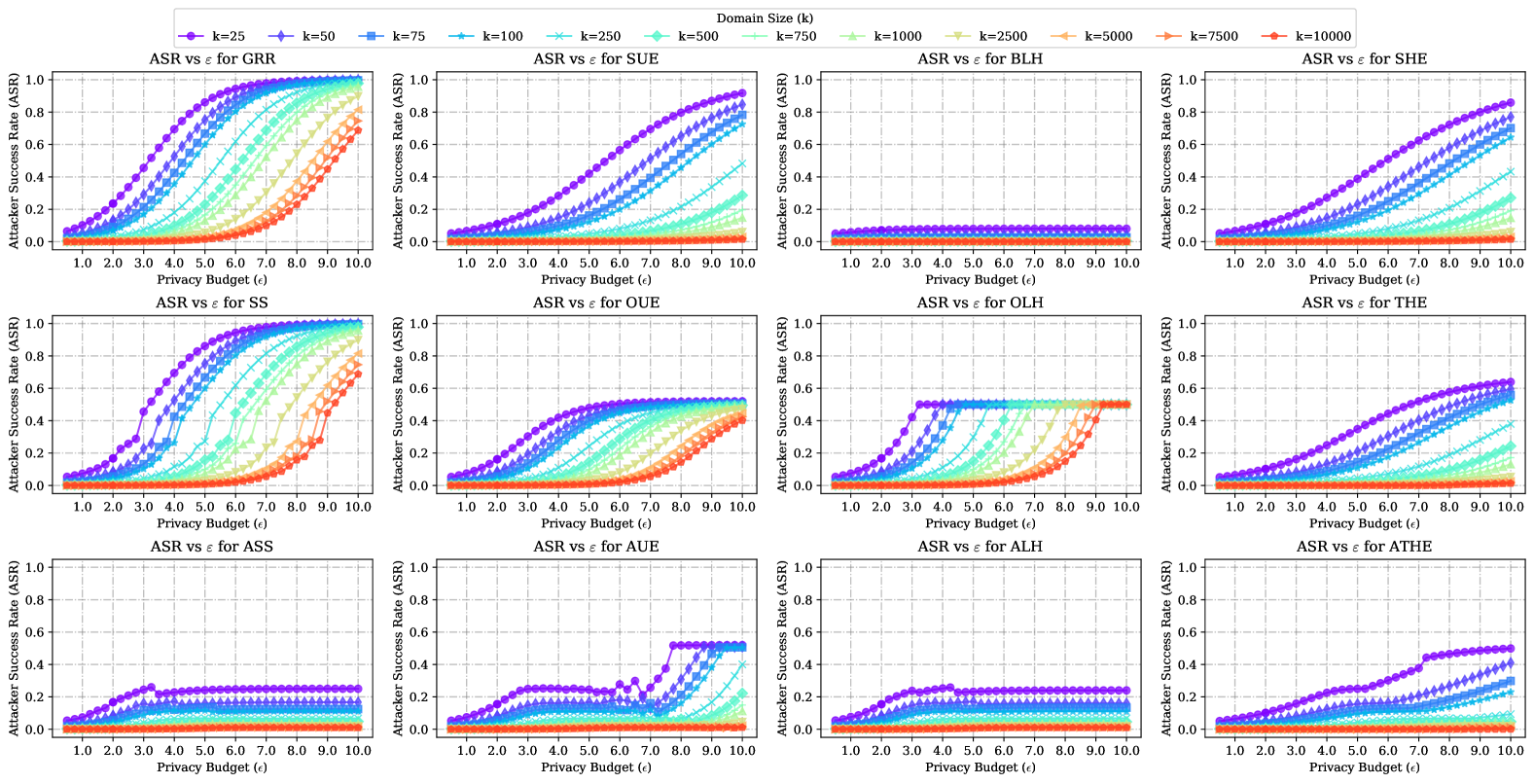
Figure 1. Attacker Success Rate (ASR) vs. privacy budget ($\varepsilon$) for different LDP frequency estimation protocols across varying domain sizes ($k$). The plots compare state-of-the-art LDP protocols, including GRR, SUE, BLH, OUE, OLH, SS, SHE, and THE, against our newly proposed adaptive protocols (ASS, AUE, ALH, ATHE). Each curve represents a different domain size, with $k$ ranging from $25$ to $10000$. The figure highlights the trade-offs between privacy and adversarial resilience for each protocol, showing how ASR evolves as the privacy budget and domain size change.

General trend across protocols: For all protocols, we observe that the ASR generally increases with increasing privacy budget $\varepsilon$ in Figure 1. This behavior is expected, as higher values of $\varepsilon$ correspond to weaker privacy guarantees, allowing the adversary to infer user data more effectively. For smaller domain sizes (i.e., $k\leq 100$, the ASR rises sharply, suggesting that the adversary’s ability to correctly guess the user’s input improves significantly as $\varepsilon$ increases. In contrast, larger domain sizes (i.e., $k\geq 1000$) show a more gradual increase in ASR, indicating that a larger domain inherently offers greater privacy protection. Nevertheless, our adaptive methods effectively counteract privacy threats regardless of $k$ and $\varepsilon$, underscoring the flexibility and robustness offered by our double-objective optimization framework.

Comparing traditional protocols: Among traditional protocols, GRR and SS demonstrate the highest ASR across all privacy budgets and domain sizes, making them the most vulnerable to privacy attacks. In contrast, SUE displays a more gradual increase in ASR, suggesting better resilience than GRR and SS. Protocols such as OUE and OLH exhibit a maximum ASR of approximately $0.5$, even as $\varepsilon$ increases, showing a clear boundary in their ASR. Notably, for SHE, ASR grows gradually as $\varepsilon$ increases, while THE’s thresholding strategy yields moderate ASR increments. Overall, BLH consistently achieves an exceptionally low ASR across all privacy budgets and domain sizes, highlighting its robustness against adversarial inference attacks.

Our refined and adaptive protocols: Our adaptive protocols (i.e., ASS, AUE, ALH, and ATHE) demonstrate significantly lower ASR compared to their traditional counterparts across all privacy budgets. For example, ASS effectively mitigates the ASR vulnerability of the state-of-the-art SS by capping the $\mathrm{ASR}$ below 0.25, in contrast to the traditional SS where the $\mathrm{ASR}$ gets to $1$ (i.e., the adversary can fully infer the user’s value). Similarly, AUE consistently achieves a lower or comparable ASR relative to the state-of-the-art OUE protocol, highlighting the benefits of its adaptive parameter optimization. For ALH, the adaptive mechanism achieves a balanced compromise between the low ASR of BLH and the moderate ASR of OLH by dynamically optimizing the hash domain size, resulting in a substantial reduction in ASR compared to traditional OLH. Finally, ATHE demonstrates more resilience than THE across all domain sizes, thereby showcasing the effectiveness of our framework in enhancing privacy protection.

ASR increases with $\varepsilon$, but our adaptive protocols resist: As the privacy budget $\varepsilon$ increases, ASR generally rises for all protocols due to weaker privacy guarantees. However, our adaptive protocols (ASS, AUE, ALH, ATHE) exhibit significantly lower (i.e., $\leq 5$ orders of magnitude) ASRs across a broad range of $\varepsilon$ values, underscoring their enhanced resilience against privacy attacks and their ability to maintain robust privacy protection.

6.3. MSE Analysis for LDP Protocols

In Figure 2, we examine the MSE behavior of the SS protocol and its adaptive counterpart ASS across varying privacy budgets $\varepsilon$. In Figure 3, we extend this analysis to compare MSE trends for UE-, LH-, and HE-based LDP protocols, including our adaptive versions (AUE, ALH, ATHE). These analyses aim to determine whether the adaptive protocols’ improved robustness to privacy attacks results in substantial estimation accuracy loss or if they maintain competitive MSE values. Notice that the MSE curves of SUE, OUE, BLH, OLH, SHE, and THE remain independent of the domain size $k$ due to their fixed parameterization, as established in previous literature (Wang et al., 2017).

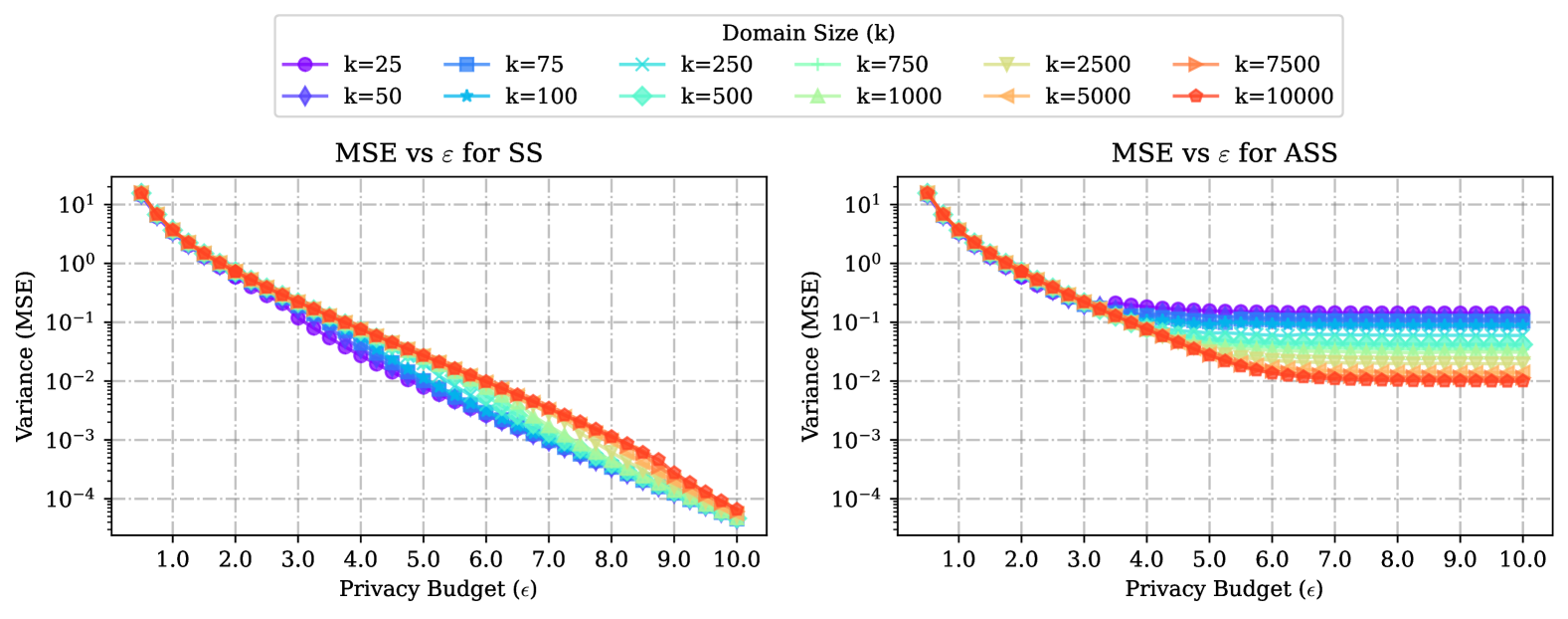
Figure 2. Variance (MSE) vs. privacy budget ($\varepsilon$) for the state-of-the-art SS protocol and our adaptive version ASS across various domain sizes $k$. Each curve represents a distinct domain size, illustrating how each protocol balances estimation accuracy with privacy as $\varepsilon$ changes.

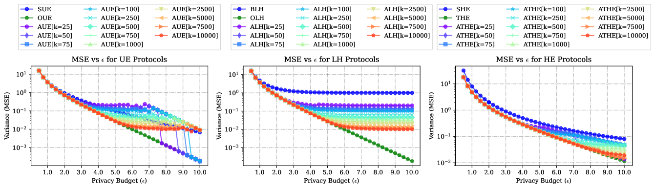
Figure 3. Variance (MSE) vs. privacy budget ($\varepsilon$) for the state-of-the-art LDP protocols (UE-, LH-, and HE-based) and our adaptive versions (AUE, ALH, and ATHE) across various domain sizes $k$. For our adaptive protocols, each curve represents a distinct domain size, illustrating how each protocol balances estimation accuracy with privacy as $\varepsilon$ changes.

For the SS protocol, we observe in Figure 2 that ASS exhibits an increase in MSE by up to two orders of magnitude compared to SS, particularly in higher privacy regimes ($\varepsilon\geq 4$). This increase is expected, as SS’s minimal MSE comes at the cost of extreme vulnerability, with ASR approaching 1 (e.g., see Figure 1), meaning an adversary can fully infer the user’s value. ASS, in contrast, balances this trade-off by introducing adaptive parameterization that mitigates privacy attacks while moderately increasing the MSE.

In Figure 3, we observe similar trends for the other adaptive protocols (AUE, ALH, and ATHE). For UE protocols, our adaptive AUE version achieves slightly higher MSE compared to OUE across all domain sizes $k$, with the gap becoming more pronounced as $\varepsilon$ increases. This is expected, as AUE optimizes its parameters to enhance robustness to privacy attacks, leading to a slight trade-off in utility. Notably, AUE remains competitive with SUE in high privacy regimes ($\varepsilon\leq 2$), offering similar MSE levels while achieving significantly improved ASR performance as shown earlier. In low privacy regimes ($\varepsilon>2$), AUE incurs a modest increase in MSE, which stays within an order of magnitude compared to OUE.

Moreover, for LH- and HE-based protocols, we observe in Figure 3 that our adaptive protocols (ALH and ATHE) demonstrate a variance (MSE) behavior that is consistently “sandwiched” between the two corresponding state-of-the-art protocols in their respective groups. Specifically, ALH achieves MSE values between those of BLH (which minimizes ASR at the cost of higher MSE) and OLH (which minimizes MSE but is more vulnerable to privacy attacks). Similarly, ATHE’s variance lies between SHE and THE, showing a trade-off where ATHE retains competitive MSE while prioritizing adversarial resilience. This positioning highlights how adaptivity allows our protocols to achieve a better privacy-utility trade-off.

Adaptive protocols maintain competitive MSE: Our adaptive protocols (ASS, AUE, ALH, ATHE) achieve higher MSE compared to their non-adaptive counterparts. However, these increases remain within acceptable bounds ($\leq 2$ orders of magnitude), highlighting that the improved adversarial resilience (ASR $\leq 5$ orders of magnitude) comes at a reasonable cost to the utility. This suggests that enhanced privacy protection against adversaries can be achieved without prohibitive increases in variance.

6.4. Pareto Frontier for ASR and MSE

In addition to evaluating how the ASR and the MSE vary with the privacy budget $\varepsilon$ separately (see Figures 1, 2 and 3), it is insightful to examine how ASR changes as a function of utility loss, measured by the variance (MSE) of the frequency estimation. Figure 4 presents the Pareto frontier between ASR and MSE for the considered LDP protocols, plotting ASR against MSE across small domain sizes and medium to low privacy regimes. This analysis highlights the performance of state-of-the-art protocols (GRR, SUE, BLH, SHE, SS, OUE, OLH, and THE) compared to our adaptive variants (ASS, AUE, ALH, and ATHE), providing insights into how effectively each method navigates the trade-off between user privacy and data utility. To address space limitations, additional results exploring the ASR-MSE trade-off under varying privacy regimes (high, medium, low) and domain sizes (small, medium, large) are provided in Appendix B. The findings and discussions in this section are supported by a comprehensive analysis that includes these extended results.

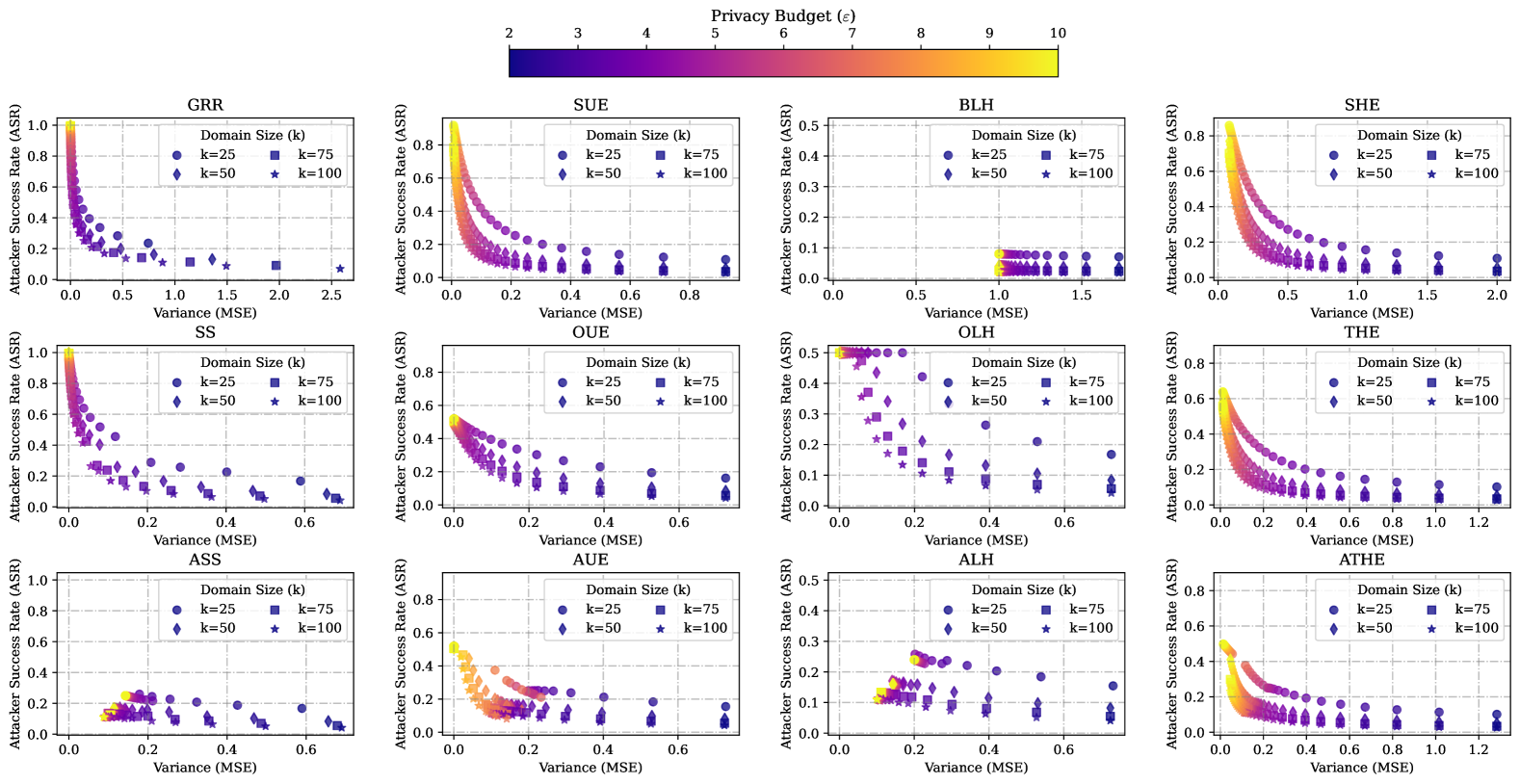
Figure 4. Attacker Success Rate (ASR) vs. Variance (MSE) for numerous LDP frequency estimation protocols. Each plot shows how each protocol performs under varying privacy budgets $\varepsilon$ and domain sizes ($k$), illustrating the trade-off between adversarial success rate (ASR) and utility (MSE). State-of-the-art LDP protocols (i.e., GRR, SUE, BLH, SHE, SS, OUE, OLH, and THE) are compared against our adaptive counterparts (i.e., ASS, AUE, ALH, and ATHE). Each point represents a different configuration of $\varepsilon$ (in medium to low privacy regimes) and $k$ (small domain), with colors indicating the privacy budget level.

General trend across protocols: For all protocols, there is a clear inverse relationship between ASR and MSE – lower variance estimates correspond to higher ASR, and vice versa. As the privacy budget $\varepsilon$ increases, protocols tend to yield estimates with lower MSE but simultaneously face higher ASRs, reflecting a direct cost to privacy when pursuing higher accuracy. Conversely, under stricter privacy regimes (lower $\varepsilon$), while ASR remains lower, the resulting estimates incur greater MSE. This fundamental tension highlights that simply tuning $\varepsilon$ does not guarantee a balanced privacy-utility outcome. Thus, understanding the ASR-MSE relationship is crucial for informed protocol selection.

Comparing traditional protocols: Among the traditional protocols, GRR and SS tend to cluster in regions with relatively lower MSE but higher ASR, especially at moderate-to-high $\varepsilon$ values. In contrast, SUE, SHE, and THE provide a more gradual trade-off curve, achieving lower ASR at slightly higher MSE levels, suggesting that these methods preserve more privacy when aiming for moderate accuracy. OUE and OLH occupy intermediate positions: they can reach points of low MSE but at the cost of increasing $\varepsilon$. BLH generally exhibits a low ASR while not bounding the MSE, indicating a low privacy-utility trade-off. Overall, none of the traditional protocols dominate the entire ASR-MSE space, and their effectiveness varies with the chosen privacy budget and domain size.

Our refined and adaptive protocols: Our adaptive protocols achieve more favorable ASR-MSE trade-offs, especially providing low-ASR even in low-privacy regimes (i.e., high $\varepsilon$ values). For instance, ASS, derived from SS, effectively prevents the sharp ASR increases observed in SS’s low-MSE regions by fine-tuning protocol parameters, resulting in points that align closer to a Pareto frontier between ASR and MSE. AUE, adapting from OUE, displays a particularly strong trade-off, often settling into low-ASR regimes without disproportionately large MSE. ALH, building on hashing-based approaches, maintains ASR reductions comparable to BLH or OLH but achieves them with more controlled MSE levels, ensuring that the benefits of hashing-based schemes are not compromised. ATHE consistently achieves configurations that lower ASR without excessively increasing MSE, indicating a more harmonious balance.

ASR-MSE trade-offs are protocol-dependent: Our findings show that each protocol exhibits a distinct ASR-MSE profile. By jointly optimizing for both privacy (ASR) and utility (MSE), our adaptive protocols consistently push these curves toward more favorable regimes in the ASR-MSE Pareto frontier.

6.5. Impact of Weights in the Objective Function

Thus far, we have focused on analyzing the performance of adaptive protocols under fixed objective configurations for the weights $(w_{\text{ASR}}=w_{\text{MSE}}=0.5)$ in Equation (23). However, our proposed multi-objective framework introduces a new degree of freedom: practitioners can adjust the relative importance of ASR vs. variance (MSE) when optimizing LDP protocols. Figure 5 illustrates how varying these weight combinations $(w_{\text{ASR}},w_{\text{MSE}})$ influences the ASR, MSE, and optimal parameter choices for AUE ($p$), ALH ($g$), ASS ($\omega$), and ATHE ($\theta$) under a fixed setting ($k=100$, $\varepsilon=4$).

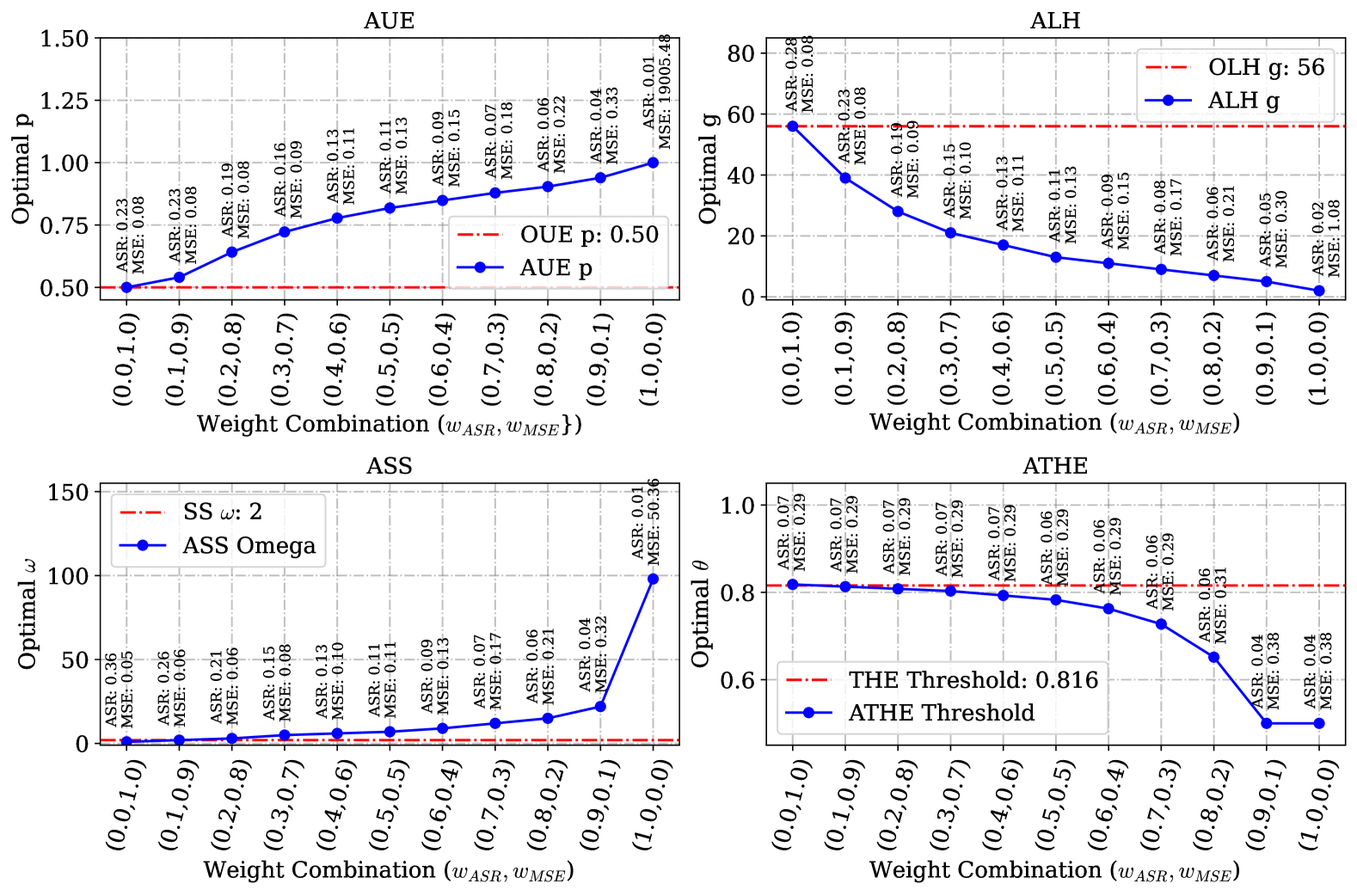
Figure 5. Optimal parameter choices for each adaptive protocol as a function of the weight combination $(w_{\text{ASR}},w_{\text{MSE}})$, evaluated at $k=100$ and $\varepsilon=4$. Each sub-figure compares the adaptive protocol’s chosen parameter (blue color curve) against the corresponding parameter choice in the original, non-adaptive protocol (red color dashed line).

From Figure 5, one can notice that as the weight on ASR $w_{\text{ASR}}$ increases, each adaptive protocol tends to choose parameter values that more aggressively reduce the ASR at the cost of increasing the MSE. Conversely, placing greater emphasis on MSE drives parameters toward configurations closer to or equal to those of the original protocols (i.e., SS, OUE, OLH, and THE), aiming to preserve utility even if it elevates the ASR. These results confirm the benefits of our two-objective optimization framework: rather than a static parameter choice, practitioners can tune the protocol parameters in response to changing priorities, achieving a more flexible trade-off between privacy (ASR) and utility (MSE).

6.6. Adaptive and Optimized Parameters

In this section, we analyze the optimization of parameters in our adaptive protocols (AUE, ALH, ASS, and ATHE) by examining the behavior of their objective functions (Equations (24)–(27)), which balance the ASR-MSE trade-off. Figure 6 illustrates the objective function as a function of key parameters: AUE ($p$), ALH ($g$), ASS ($\omega$), and ATHE ($\theta$), with a fixed $k=100$ and $\varepsilon=4$. The selected parameters for our adaptive protocols are compared against the fixed state-of-the-art parameters of OUE, OLH, SS, and THE.

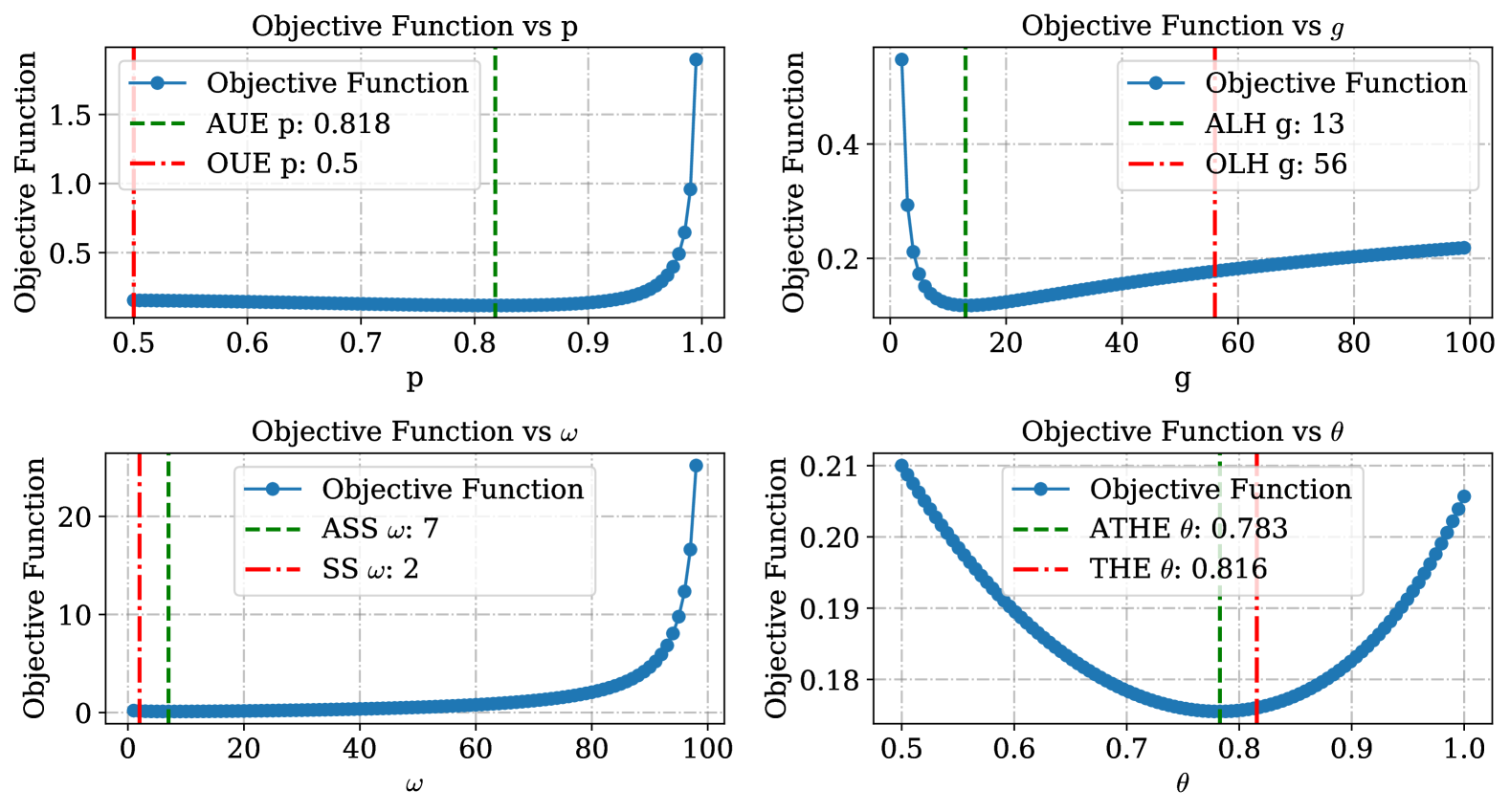
Figure 6. Objective function value as a function of key parameters for our adaptive protocols (AUE, ALH, ASS, and ATHE) compared with their state-of-the-art counterparts (OUE, OLH, SS, and THE). Vertical dashed lines (green color) indicate the optimal parameter values selected by our adaptive protocols, while vertical dash-dotted lines (red color) represent the fixed parameter values of the state-of-the-art protocols. Without loss of generality, we set $k=100$ and $\varepsilon=4$.

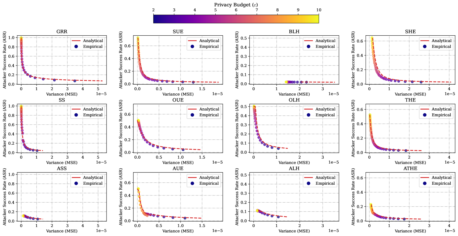
Figure 7. Comparison of empirical and analytical Pareto frontiers for ASR vs. Variance (MSE) across various LDP protocols (state-of-the-art and adaptive). Each subplot considers a range of privacy budgets $\varepsilon\in(2,10)$ and a fixed domain size $k=100$. Empirical results ($\circ$ makers) are averaged over $100$ independent runs with the Age attribute of the Adult dataset (Dua and Graff, 2017), while analytical results (red dashed lines) are computed using closed-form equations.

For AUE, we observe in the top-left plot that the objective function reaches its minimum at $p=0.818$, which is notably higher than the fixed $p=0.5$ used by OUE. This also means that parameter $q$ will increase to satisfy $\varepsilon$-LDP, i.e., increasing the probability of reporting random bits. For ALH, as shown in the top-right plot, the optimal hash domain size is reduced to $g=13$ in our adaptive protocol compared to $g=56$ in OLH. This reduction in $g$ lowers the ASR at the expense of slightly increased variance, aligning with our adaptive objective to achieve a better balance between privacy and utility. For ASS, as depicted in the bottom-left plot, the optimal subset size $\omega=7$ contrasts with the fixed $\omega=2$ used in SS. The larger $\omega$ effectively spreads the probability mass across a larger subset, reducing ASR while incurring a higher variance. For ATHE, the bottom-right plot shows that the adaptive threshold $\theta=0.783$ is slightly lower than the fixed threshold $\theta=0.816$ in THE. This subtle adjustment enables ATHE to reduce privacy attacks while maintaining competitive variance levels, showcasing the precision of our adaptive optimization.

Adaptive protocols optimize key parameters for better trade-offs: Our findings demonstrate that the optimized parameters selected by adaptive protocols significantly differ from the fixed parameters of state-of-the-art protocols, resulting in improved robustness to privacy attacks with controlled increases in variance. This optimization highlights the flexibility and effectiveness of our adaptive mechanisms in better navigating the privacy-utility trade-off space.

6.7. Empirical Pareto Frontier for ASR and MSE

To assess the accuracy of our closed-form ASR and MSE equations within the ASR-MSE two-objective framework (Section 5.2), we conduct empirical experiments using the Adult dataset from the UCI machine learning repository (Dua and Graff, 2017). We select the Age attribute with domain size $k=100$ (i.e., $\text{Age}\in[0,99]$) and $n=48842$ users, reporting results averaged over $100$ independent runs.

Figure 7 presents the comparison between empirical ($\circ$ makers) and analytical (red dashed lines) Pareto frontiers for ASR versus MSE across various LDP protocols, including both state-of-the-art and our adaptive variants. Each subplot represents a specific protocol (i.e., GRR, SUE, BLH, SHE, SS, OUE, OLH, THE, ASS, AUE, ALH and ATHE) with the privacy budget varying as $\varepsilon\in(2,10)$ with the domain size fixed at $k=100$. One can notice that across all protocols, the empirical results closely align with the analytical calculation, showcasing the robustness of the closed-form equations for ASR and MSE. This alignment highlights the reliability of our theoretical framework and previous analytical experiments across different privacy budgets and data distributions. To further support this claim, Appendix C provides additional experiments using a synthetic dataset generated from a Dirichlet distribution ($\mathbf{1}$), exploring variations in the number of users ($n\in\{5000,50000,500000\}$).

Analytical vs. empirical validation: Our findings demonstrate that the analytical results closely align with empirical ones, reaffirming the reliability of the closed-form equations across various privacy budgets and scenarios.

7. Conclusion and Perspectives

In this work, we introduced a general multi-objective optimization framework for refining LDP frequency estimation protocols, enabling adaptive parameter tuning based on multiple privacy and utility considerations. While the classical LDP paradigm primarily focuses on minimizing the estimation error (i.e., utility-driven), our framework provides a flexible optimization approach that balances multiple objectives in adversarial settings. As an instantiation of this framework, we focused on a two-objective formulation that jointly minimizes the Attacker Success Rate (ASR) under distinguishability attacks (Emre Gursoy et al., 2022; Arcolezi et al., 2023a; Arcolezi and Gambs, 2024) and Mean Squared Error (MSE), demonstrating that existing protocols (i.e., SS, OUE, OLH and THE) can be beneficially re-optimized. Our adaptive protocols, namely, ASS, AUE, ALH and ATHE, significantly reduce adversarial success rates while maintaining competitive estimation accuracy (e.g., see Figure 4).

Beyond this specific instantiation, our findings pave the way for broader applications of our framework. First, our approach naturally extends to alternative privacy, utility and security objectives, such as robustness to poisoning attacks (Cao et al., 2021; Cheu et al., 2021), resilience against inference (GÜRSOY, 2024; Arcolezi et al., 2023b) and re-identification (Murakami and Takahashi, 2021; Arcolezi et al., 2023a) risks or the integration of entropy-based utility metrics (Barnes et al., 2020). Additionally, incorporating constraints on communication cost and efficiency would enhance its applicability to real-world, resource-constrained environments. Finally, we envision the development of an LDP optimization suite that accommodates various objectives, such as constrained utility, constrained $\varepsilon$, double-objective problems, and so on. This suite could serve as a practical tool for deploying LDP mechanisms tailored to specific real-world requirements.

Appendix A Expected ASR Analyses

A.1. UE Protocols

Following the attack strategy for UE in Section 4.3, we consider two events:

• Event 0: The bit corresponding to the user’s value $x$ is flipped from 1 to 0, and all other bits remain 0.

  • The attacker’s guess is uniformly distributed over all $k$ possible values.

  • Success rate: $\frac{1}{k}$.

  • Probability: $\Pr(\text{Event 0})=(1-p)(1-q)^{k-1}$.

• Event 1: The bit corresponding to the user’s value $x$ remains 1, and $m-1$ of the remaining $k-1$ bits are flipped from 0 to 1.

  • The attacker’s guess is uniformly distributed over the bits set to 1.

  • If $m$ bits are set to 1, the success rate is $\frac{1}{m}$.

  • Probability: $\Pr(\text{Event 1 with }m\text{ bits set to 1})=\binom{k-1}{m-1}p(q)^{m-1}(1-q)^{k-m}$.

Thus, combining these two events, we can derive the expected ASR as:

$$\mathbb{E}[\text{ASR}]_{\mathrm{UE}}=\Pr(\text{Event 0})\cdot\frac{1}{k}+\sum_{m=1}^{k}\Pr(\text{Event 1 with }m\text{ bits set to 1})\cdot\frac{1}{m}\mathrm{.}$$

More formally, the probability calculations of each event are:

1. Probability of Event 0:

   $$\Pr(\text{Event 0})=(1-p)(1-q)^{k-1}\mathrm{.}$$

2. Probability of Event 1 with $m$ bits set to 1:

   $$\Pr(\text{Event 1 with }m\text{ bits set to 1})=\binom{k-1}{m-1}p(q)^{m-1}(1-q)^{k-m}\mathrm{.}$$

Combining these probabilities, the expected ASR for UE is:

$$\mathbb{E}[\text{ASR}]_{\mathrm{UE}}= \,(1-p)\cdot(1-q)^{k-1}\cdot\frac{1}{k}$$

$$+\sum_{m=1}^{k}p\cdot\frac{1}{m}\cdot\binom{k-1}{m-1}q^{m-1}(1-q)^{(k-1)-(m-1)}\mathrm{.}$$

A.2. SHE Protocol

The expected ASR of SHE is defined as the probability that $\hat{x}=x$:

$$\mathbb{E}[\text{ASR}]_{\mathrm{SHE}}=\Pr[\hat{x}=x]=\Pr\left[y_{x}>\max_{i\neq x}y_{i}\right]\mathrm{.}$$

Define the random variables:

$$y_{x} =1+Z_{x},\quad\text{where }Z_{x}\sim\text{Laplace}(0,b)\mathrm{,}$$

$$y_{i} =0+Z_{i}=Z_{i},\quad\text{where }Z_{i}\sim\text{Laplace}(0,b)\mathrm{,}\quad\forall i\neq x$$

All $Z_{i}$ and $Z_{x}$ are independent random variables. Let $M=\max_{i\neq x}y_{i}=\max_{i\neq x}Z_{i}$. Then, the expected ASR becomes:

$$\mathbb{E}[\text{ASR}]_{\mathrm{SHE}}=\Pr\left[y_{x}>M\right]=\Pr\left[1+Z_{x}>M\right]=\Pr\left[Z_{x}>M-1\right]\mathrm{.}$$

The cumulative distribution function (CDF) of the Laplace distribution $Z_{x}\sim\text{Laplace}(0,b)$ is:

$$F_{Z}(z)=\begin{cases}\dfrac{1}{2}\exp\left[\dfrac{z}{b}\right],&\text{if }z\leq 0\mathrm{,}\\ 1-\dfrac{1}{2}\exp\left[-\dfrac{z}{b}\right],&\text{if }z>0\mathrm{.}\end{cases}$$

The probability density function (PDF) of $Z_{x}$ is:

$$f_{Z}(z)=\dfrac{1}{2b}\exp\left[-\dfrac{|z|}{b}\right]\mathrm{.}$$

For $M=\max_{i\neq x}Z_{i}$, since $Z_{i}$ are independent and identically distributed (i.i.d.), the CDF of $M$ is:

(28) $$F_{M}(m)=\left[F_{Z}(m)\right]^{k-1}\mathrm{.}$$

The PDF of $M$ is then:

(29) $$f_{M}(m)=(k-1)\left[F_{Z}(m)\right]^{k-2}f_{Z}(m)\mathrm{.}$$

The ASR can be expressed as:

(30) $$\mathbb{E}[\text{ASR}]_{\mathrm{SHE}}=\int_{-\infty}^{\infty}\Pr\left[Z_{x}>m-1\right]f_{M}(m)\,dm\mathrm{.}$$

Since $Z_{x}$ and $M$ are independent, $\Pr\left[Z_{x}>m-1\right]=1-F_{Z}(m-1)$. Therefore:

(31) $$\mathbb{E}[\text{ASR}]_{\mathrm{SHE}}=\int_{-\infty}^{\infty}\left[1-F_{Z}(m-1)\right]f_{M}(m)\,dm\mathrm{.}$$

Empirical Estimation via Simulation. In this work, we estimate the expected ASR in Equation (31) empirically using Monte Carlo simulations, following:

1. Generate Samples:

   • Sample $Z_{x}$ from $\text{Laplace}(0,b)$.

   • Sample $Z_{i}$ for $i\neq x$ and compute $M=\max_{i\neq x}Z_{i}$.

2. Compute Success Indicator:

   • For each sample, check if $1+Z_{x}>M$.

3. Estimate ASR:

   • The ASR is estimated as the proportion of times $1+Z_{x}>M$ holds over all samples.

A.3. THE Protocol

Following the attack strategy for THE in Section 4.5.2, we have:

• Event 0: The bit corresponding to the user’s value $x$ is less than $\theta$ (i.e., remains 0) and all other bits also remain 0.

  • The attacker’s guess is uniformly distributed over all $k$ possible values.

  • Success rate: $\frac{1}{k}$.

  • Probability: $\Pr(\text{Event 0})=(1-p)(1-q)^{k-1}$.

• Event 1: The bit corresponding to the user’s value $x$ is greater than $\theta$ (i.e., flips to 1) and $m-1$ other bits also flip to 1.

  • The attacker’s guess is uniformly distributed over the bits set to 1.

  • If $m$ bits are set to 1, the success rate is $\frac{1}{m}$

  • Probability: $\Pr(\text{Event 1 with }m\text{ bits set to 1})=\binom{k-1}{m-1}p(q)^{m-1}(1-q)^{k-m}$.

Thus, by combining these two events, we can derive the expected ASR as:

$$\mathbb{E}[\text{ASR}]_{\mathrm{THE}}=\Pr(\text{Event 0})\cdot\frac{1}{k}+\sum_{m=1}^{k}\Pr(\text{Event 1 with }m\text{ bits set to 1})\cdot\frac{1}{m}\mathrm{.}$$

More formally, the probability calculations of each event are:

1. Probability of Event 0:

   $$\Pr(\text{Event 0})=(1-p)(1-q)^{k-1}\mathrm{.}$$

2. Probability of Event 1 with $m$ bits set to 1:

   $$\Pr(\text{Event 1 with }m\text{ bits set to 1})=\binom{k-1}{m-1}p(q)^{m-1}(1-q)^{k-m}\mathrm{.}$$

Combining these probabilities, the expected ASR for THE is:

$$\mathbb{E}[\text{ASR}]_{\mathrm{THE}}=(1-p)(1-q)^{k-1}\cdot\frac{1}{k}+\sum_{m=1}^{k}\binom{k-1}{m-1}p(q)^{m-1}(1-q)^{k-m}\cdot\frac{1}{m}\mathrm{.}$$

Appendix B Additional Analytical Results for the ASR vs. MSE Trade-Off

To complement the results of Figure 4 (medium to low privacy regimes and small domain size) in Section 6.4, Figures 8 to 12 illustrates the ASR-MSE trade-off considering:

• Figure 8: high privacy regime and small domain size.

• Figure 9: high privacy regime and medium domain size.

• Figure 10: high privacy regime and large domain size.

• Figure 11: medium to low privacy regimes and medium domain size.

• Figure 12: medium to low privacy regimes and large domain size.

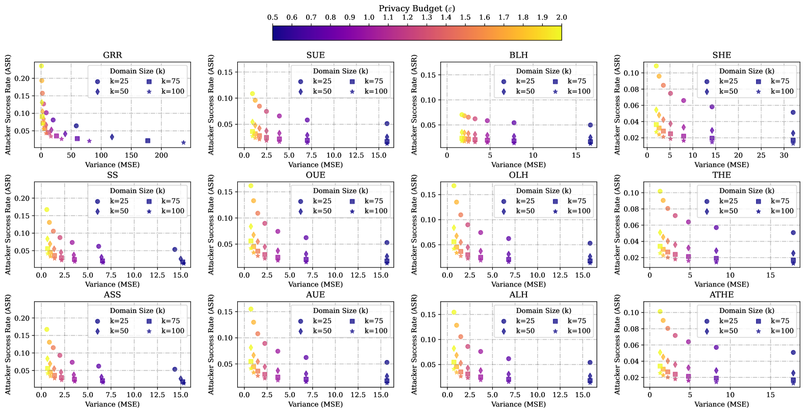
Figure 8. Attacker Success Rate (ASR) vs. Variance (MSE) for numerous LDP frequency estimation protocols. Each plot shows how each protocol performs under varying privacy budgets $\varepsilon$ and domain sizes ($k$), illustrating the trade-off between adversarial success rate (ASR) and utility (MSE). State-of-the-art LDP protocols (i.e., GRR, SUE, BLH, SHE, SS, OUE, OLH, and THE) are compared against our adaptive counterparts (i.e., ASS, AUE, ALH, and ATHE). Each point represents a different configuration of $\varepsilon$ (in high privacy regimes) and $k$ (small domain), with colors indicating the privacy budget level.

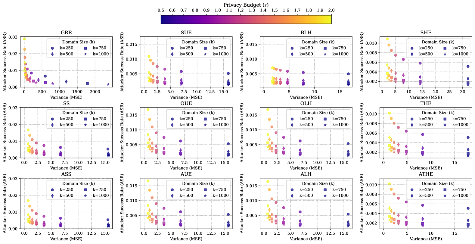
Figure 9. Attacker Success Rate (ASR) vs. Variance (MSE) for numerous LDP frequency estimation protocols. Each plot shows how each protocol performs under varying privacy budgets $\varepsilon$ and domain sizes ($k$), illustrating the trade-off between adversarial success rate (ASR) and utility (MSE). State-of-the-art LDP protocols (i.e., GRR, SUE, BLH, SHE, SS, OUE, OLH, and THE) are compared against our adaptive counterparts (i.e., ASS, AUE, ALH, and ATHE). Each point represents a different configuration of $\varepsilon$ (in high privacy regimes) and $k$ (medium domain), with colors indicating the privacy budget level.

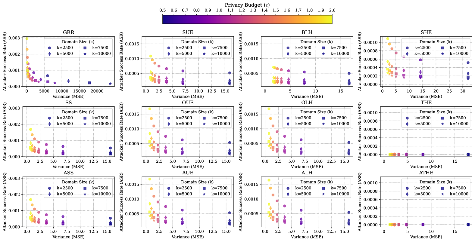
Figure 10. Attacker Success Rate (ASR) vs. Variance (MSE) for numerous LDP frequency estimation protocols. Each plot shows how each protocol performs under varying privacy budgets $\varepsilon$ and domain sizes ($k$), illustrating the trade-off between adversarial success rate (ASR) and utility (MSE). State-of-the-art LDP protocols (i.e., GRR, SUE, BLH, SHE, SS, OUE, OLH, and THE) are compared against our adaptive counterparts (i.e., ASS, AUE, ALH, and ATHE). Each point represents a different configuration of $\varepsilon$ (in high privacy regimes) and $k$ (large domain), with colors indicating the privacy budget level.

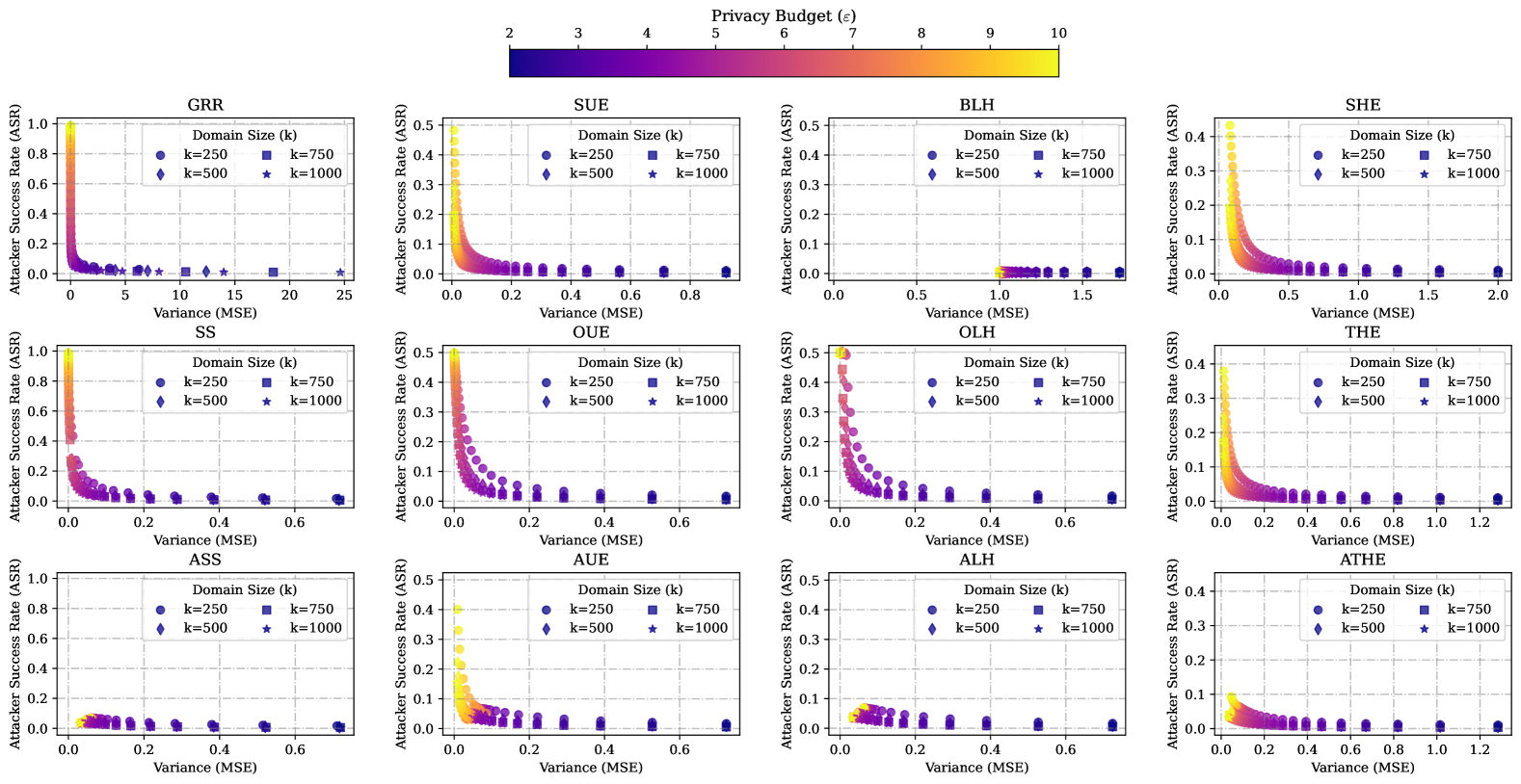
Figure 11. Attacker Success Rate (ASR) vs. Variance (MSE) for numerous LDP frequency estimation protocols. Each plot shows how each protocol performs under varying privacy budgets $\varepsilon$ and domain sizes ($k$), illustrating the trade-off between adversarial success rate (ASR) and utility (MSE). State-of-the-art LDP protocols (i.e., GRR, SUE, BLH, SHE, SS, OUE, OLH, and THE) are compared against our adaptive counterparts (i.e., ASS, AUE, ALH, and ATHE). Each point represents a different configuration of $\varepsilon$ (in medium to low privacy regimes) and $k$ (medium domain), with colors indicating the privacy budget level.

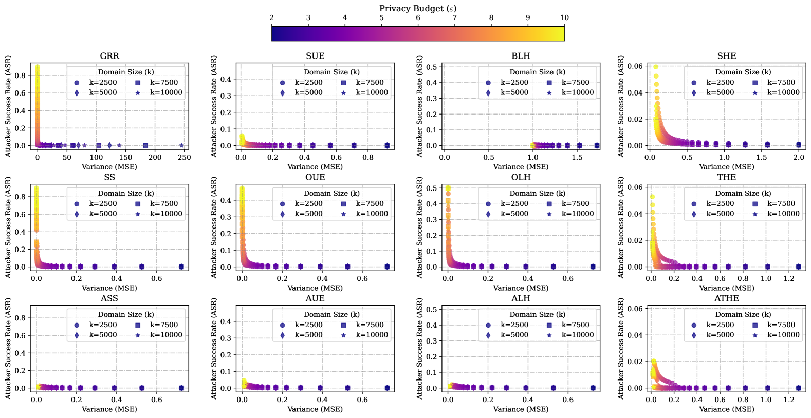
Figure 12. Attacker Success Rate (ASR) vs. Variance (MSE) for numerous LDP frequency estimation protocols. Each plot shows how each protocol performs under varying privacy budgets $\varepsilon$ and domain sizes ($k$), illustrating the trade-off between adversarial success rate (ASR) and utility (MSE). State-of-the-art LDP protocols (i.e., GRR, SUE, BLH, SHE, SS, OUE, OLH, and THE) are compared against our adaptive counterparts (i.e., ASS, AUE, ALH, and ATHE). Each point represents a different configuration of $\varepsilon$ (in medium to low privacy regimes) and $k$ (large domain), with colors indicating the privacy budget level.

Appendix C Additional Empirical Results for the ASR vs. MSE Trade-Off

To complement the results presented in Figure 7 (Adult dataset (Dua and Graff, 2017) with $n=48842$ and $k=100$ for the Age attribute), we now conduct experiments using a synthetic dataset generated from a Dirichlet distribution with parameter $\mathbf{1}$. Specifically, we compare empirical results obtained with varying numbers of users against analytical predictions computed using our closed-form equations from Section 5.3. Figure 13 presents the analytical Pareto frontier for ASR vs. MSE for SS, OUE, OLH, and THE against our adaptive counterparts, i.e., ASS, AUE, ALH, and ATHE, providing a baseline for evaluating the empirical results. Meanwhile, Figure 14 presents the empirical Pareto frontiers for the same protocols across different user counts ($n\in\{5000,50000,500000\}$). Each subplot of Figures 13 and 14 evaluates the trade-off between ASR and MSE under varying privacy budgets $\varepsilon\in(2,10)$ and a fixed domain size $k=100$.

Consistency across user counts: Notably, Figure 14 shows that while the absolute variance (MSE) scales inversely with the number of users, the overall shape of the ASR-MSE Pareto frontier remains consistent across different values of $n$. This behavior aligns with theoretical expectations, as increasing the number of users reduces the variance but does not alter the fundamental trade-off between privacy and utility.

Empirical and analytical alignment: Similar to the results in Figure 7, the empirical ASR-MSE trends in Figure 14 closely follow the analytical ones in Figure 13, reinforcing the validity of our closed-form equations across various dataset distributions and user settings. These findings confirm that our analytical framework provides a reliable approximation for real-world deployments of LDP protocols, allowing practitioners to anticipate privacy-utility trade-offs without requiring extensive empirical evaluations.

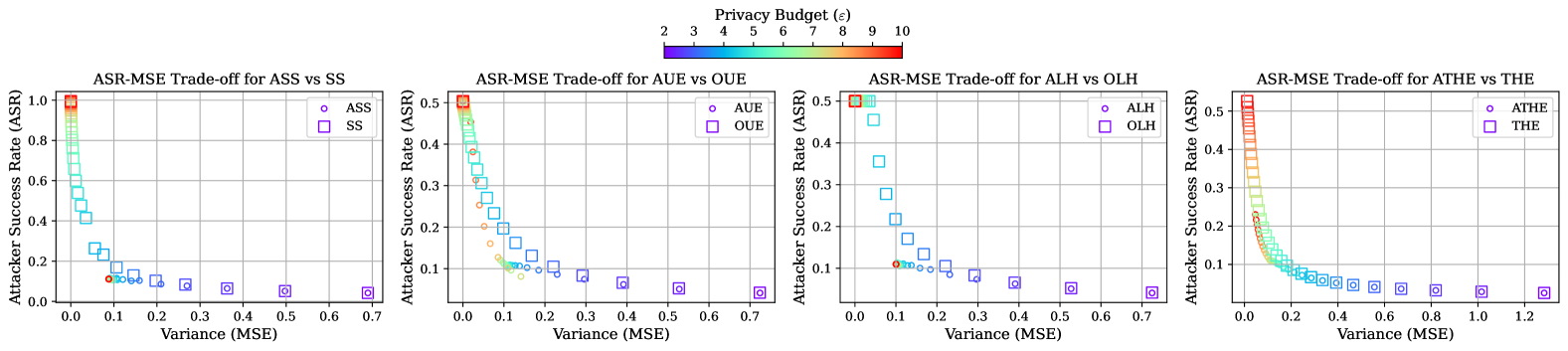
Figure 13. Analytical comparison of ASR vs. MSE Pareto frontier for four state-of-the-art LDP protocols (i.e., SS, OUE, OLH, and THE) and our proposed adaptive versions (i.e., ASS, AUE, ALH, ATHE). Each subplot considers a range of privacy budgets $\varepsilon\in(2,10)$ and a fixed domain size $k=100$.

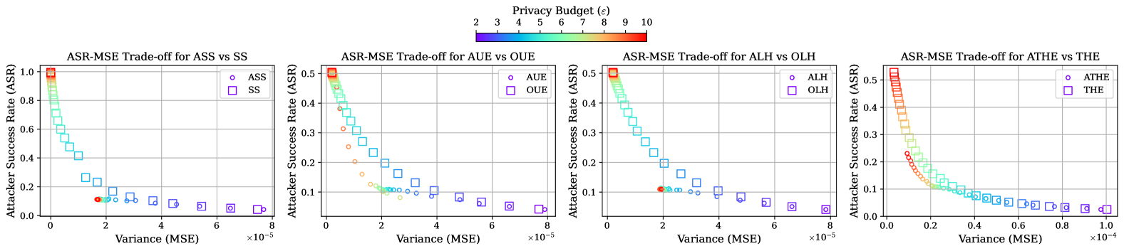
(a) Number of users $n=5000$.

(b) Number of users $n=50000$.

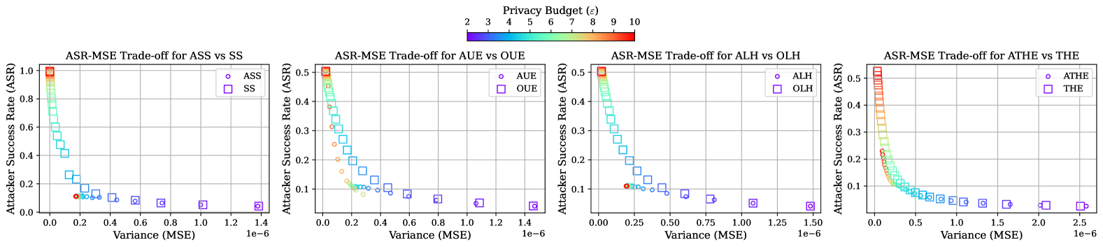
(c) Number of users $n=500000$.

Figure 14. Empirical comparison of ASR vs. MSE Pareto frontier for four state-of-the-art LDP protocols (i.e., SS, OUE, OLH, and THE) and our proposed adaptive versions (i.e., ASS, AUE, ALH, ATHE). Each subplot considers a range of privacy budgets $\varepsilon\in(2,10)$, a fixed domain size $k=100$, and varying numbers of users $n\in\{5000,50000,500000\}$. The dataset follows a Dirichlet distribution with parameter $\mathbf{1}$. Results are averaged over $100$ independent runs.