Provably optimal decision trees with arbitrary splitting rules in polynomial time

Abstract.

In this paper, we introduce a generic data structure called decision trees, which integrates several well-known data structures, including binary search trees, $K$-D trees, binary space partition trees, and decision tree models from machine learning. We provide the first axiomatic definition of decision trees. These axioms establish a firm mathematical foundation for studying decision tree problems. We refer to decision trees that satisfy the axioms as proper decision trees. We prove that only proper decision trees can be uniquely characterized as $K$-permutations. Since permutations are among the most well-studied combinatorial structures, this characterization provides a fundamental basis for analyzing the combinatorial and algorithmic properties of decision trees.

As a result of this advancement, we develop the first provably correct polynomial-time algorithm for solving the optimal decision tree problem. Our algorithm is derived using a formal program derivation framework, which enables step-by-step equational reasoning to construct side-effect-free programs with guaranteed correctness. The derived algorithm is correct by construction and is applicable to decision tree problems defined by any splitting rules that adhere to the axioms and any objective functions that can be specified in a given form. Examples include the decision tree problems where splitting rules are defined by axis-parallel hyperplanes, arbitrary hyperplanes, hypersurfaces. By extending the axioms, we can potentially address a broader range of problems. Moreover, the derived algorithm can easily accommodate various constraints, such as tree depth and leaf size, and is amenable to acceleration techniques such as thinning method.

Our results contradict several unproven claims in the literature, such as the incorrect characterization of decision trees that fail to satisfy the axioms as K-permutations, and the use of Catalan number-style recursion in solving decision tree problems. More importantly, we demonstrate that, while a dynamic programming recursion exists for this problem, the use of memoization is generally impractical in terms of space complexity. This finding questions the application of memoization techniques commonly used in the study of decision tree problems with binary feature data.

1. Introduction

A binary search tree (BST), also known as an ordered or sorted binary tree, is a rooted binary tree data structure constructed by comparing the keys of branch nodes with those of their subtree nodes. Specifically, the key of each branch node is greater than all keys in its left subtree and less than all keys in its right subtree. This comparison is based on a total order over one-dimensional objects, such as real numbers or integers. The decision tree generalizes the BST, with both structures designed for efficient information retrieval. Unlike the BST, which is constrained to a total order, the decision tree accommodates “comparisons” involving non-total orders for multi-dimensional objects. We will refer to the “comparisons” in a decision tree as splitting rules, which will be formally defined in later discussions. Additionally, in a BST, both leaf and branch nodes share the same type, while decision trees allow for distinct types for branch and leaf nodes. Due to the generality of the decision tree data structure, it encompasses tree-like structures across various domains. For example, the binary space partitioning tree (Tóth, 2005; De Berg, 2000) and the $K$-D-tree (Bentley, 1975) in computational geometry, as well as the decision tree model in machine learning (Breiman et al., 1984), are all special cases of the decision tree introduced in this paper.

It may be more appropriate to illustrate the decision tree in the context of machine learning, where there are typically no strict restrictions on the most suitable model. In this setting, any splitting rule can be applied, providing greater flexibility in constructing the tree. In contrast, in certain applications, such as the application of using $K$-D tree and binary space partition tree, the decision tree data structure may be constrained by specific requirements that limit the choice of splitting rules.

In machine learning, a decision tree is a model that can be applied to both supervised and unsupervised learning problems, known as classification trees and regression trees, respectively. It makes predictions by subdividing the feature space through a tree-based structure. Consider a flowchart or a series of “yes” or “no” questions that guide towards a final prediction decision. Geometrically, each question or condition at a node in the tree, splits the feature data into two groups based on a feature’s value, these splits are parallel to the axis of the feature space. For instance, at each node, the tree asks a question about a single feature: “Is feature $x_{d}$ greater than some value $v$?” This question divides the feature space into two regions, $x_{d}\leq v$ and $x_{d}>v$, through hyperplanes parallel to the axis, $x_{d}=0$. Due to the unparalleled simplicity and interpretability of the decision tree model, algorithms that can learn an accurate decision tree model—for instance, classification and regression trees (CART) (Breiman et al., 1984), C4.5 (Quinlan, 2014) and random forests (Breiman, 2001a)—are very widely used across various fields. Breiman (2001b) aptly noted, “On interpretability, trees rate an A+.”

The classical heuristic algorithms for creating decision trees, such as CART and C4.5, usually use a top-down, greedy approach. As a result, these approximate algorithms do not guarantee finding the global optimal solution. A global optimal solution, sometimes referred to as the optimal or exact solution, is the best possible solution to a problem with respect to a prespecified objective function. Algorithms that are guaranteed to find an optimal solution (or several with equivalent objectives) are called exact or optimal algorithms. We will use “exact” and “optimal” interchangeably in the following discussion. In the study of classification problems in machine learning, the final comparison is almost always based on one objective—the number of misclassifications—although this combinatorial objective is rarely directly optimized due to the inherent difficulty of optimizing such combinatorial objectives.

To improve the accuracy of the decision tree model, there are two common approaches. One is to find the globally optimal axis-parallel decision tree that minimizes the number of misclassifications. Alternatively, instead of constructing models that create axis-parallel hyperplanes, more complex splitting rules can be applied. For example, a generalization of the classical decision tree problem is the hyperplane (or oblique) decision tree, which uses hyperplane decision boundaries to potentially simplify boundary structures. The axis-parallel tree model is very restrictive in many situations. Indeed, it is easy to show that axis-parallel methods will have to approximate the true underlying decision boundary with a “staircase-like” structure. By contrast, the tree generated using hyperplane splits is often smaller and more accurate than the axis-parallel tree. It should be intuitively clear that when the true, underlying decision regions are defined by a polygonal space partition (such as that described by non-axis aligned hyperplane boundaries) it is preferable to use hyperplane decision trees for classification. By contrast, the axis-parallel tree model can only produce hyper-rectangular decision regions. Figure 7 depicts three different decision tree models—the axis-parallel decision tree, the hyperplane decision tree, and the hypersurface decision tree (defined by a degree-two polynomial)—to classify the same dataset. As the complexity of the splitting rule increases, the resulting decision tree becomes simpler and more accurate.

However, finding the optimal solution for the axis-parallel tree model and optimizing the hyperplane decision tree are both extremely difficult. It is well-known that the problem of finding the smallest axis-parallel decision tree is NP-hard Laurent and Rivest (1976). Similarly, for the hyperplane decision tree problem, even the top-down, inductive greedy optimization approach—similar to the CART algorithm—is NP-hard. This is a consequence of the fact that the 0-1 loss linear classification problem is NP-hard. As Murthy et al. (1994) explained, “But when the tree uses oblique splits, it is not clear, even for a fixed number of attributes, how to generate an optimal decision tree in polynomial time.”

Due to the formidable combinatorial complexity of decision tree problems, studies on decision tree problems focus on either designing good approximate algorithms (Wickramarachchi et al., 2016; Barros et al., 2011; Cai et al., 2020) or developing exact algorithms that produce trees with specific structures, such as the complete binary tree of a given depth, known as BinOCT Verwer and Zhang (2019). In particular, a substantial number of studies have focused on optimal decision tree algorithms for datasets with binary features (Lin et al., 2020; Hu et al., 2020; Aglin et al., 2021, 2020; Nijssen and Fromont, 2007, 2010; Zhang et al., 2023). This problem has a combinatorial complexity that is independent of the input data size, as the number of splitting rules depends solely on the number of possible features, thus it is polynomially solvable. On the other hand, exact algorithms addressing the axis-parallel decision tree problem in full generality primarily use mixed-integer programming (MIP) solvers (Aghaei et al., 2019; Mazumder et al., 2022; Aghaei et al., 2021; Bertsimas and Dunn, 2017; Günlük et al., 2021). For example, Bertsimas and Dunn (2017) employed MIP solvers for the hyperplane decision tree problem. However, it is well-known that MIP solvers have exponential (or worse) complexity in the worst case. Bertsimas and Dunn (2019) reported that their algorithm, based on MIP solvers, quickly becomes intractable when increasing the number of branch nodes. Additionally, Hu et al. (2019) observed that one solution presented in the figures of Bertsimas and Dunn (2017)’s is sub-optimal. However, since Bertsimas and Dunn (2017) did not release their code publicly, it remains unclear why their algorithm returns a sub-optimal solution. This suggests that Bertsimas and Dunn (2017)’s algorithm may not be exact, and our algorithm, presented in this paper, may be the only one capable of solving the hyperplane decision tree problem exactly.

In this paper, we solve the optimal decision tree problem in a way which is provably correct, based on a rigorous, axiomatic treatment. To the best of our knowledge, no such provably correct solution has been presented, and most solutions to the relaxed problems—those augmented with additional constraints to simplify optimization—are incorrect. More importantly, even when compared to potentially incorrect algorithms, our novel algorithm is the fastest, in terms of worst-case complexity.

The axiomatic treatment of decision trees offers several advantages. Firstly, it establishes the topic on a solid mathematical foundation. We demonstrate that only decision trees that satisfy the axioms (which we refer to as proper decision trees) can be characterized as $K$-permutations through a level-order traversal of the tree. Such $K$-permutations are then called valid $K$-permutations. Secondly, permutations are among the most well-studied combinatorial objects. As (Sedgewick, 1977) noted, “Perhaps more algorithms have been developed for generating permutations than any other kind of combinatorial structure.” This wealth of knowledge about permutations provides a solid basis for designing efficient programs to solve the optimal decision tree (ODT) problem. Thirdly, the axioms are general, encompassing a wide range of decision tree problems, including axis-parallel, hyperplane, and hypersurface decision tree problems. Furthermore, by extending the axioms, we have the potential to address an even broader range of problems. Finally, our rigorous characterization exposes several erroneous claims in the existing literature. For example, Hu et al. (2019), wrongly characterize their tree as $K$-permutations, because the decision tree over binary feature data does not satisfy the axioms presented here, hence cannot be characterized as $K$-permutations.

Algorithm designers often omit certain implementation details, leading to a gap between the abstract algorithm and its concrete implementation. By contrast, within the constructive algorithmics community (Bird and De Moor, 1996; de Moor and Gibbons, 1999; Bird, 1987, 2010; Bird and Gibbons, 2020), it is common to see formal developments of textbook algorithms that focus on design by logical derivation. These derivations typically proceed all the way to a complete concrete implementation, i.e. runnable code, although the resulting solution may be less efficient than more ad-hoc code (de Moor and Gibbons, 1999).

This paper represents a further exploration of constructive algorithmics (or program calculus) to address novel problems. We argue that employing a formal framework, such as the algebra of programming formalism proposed by Bird and De Moor (1996); Bird (2010), is essential for designing exact algorithms. The necessity of this approach becomes evident when considering how easily errors can arise without step-by-step equational reasoning. To effectively apply equational reasoning for program calculation, one must define all foundational elements—such as the minimization function $\mathit{min}$ and the objective function $E$—explicitly through programmatic specifications. Only by unambiguously establishing these components can we ensure the absence of errors, as the derivations are fully transparent and start from a clear, unambiguous specification. Admittedly, this rigorous process complicates the development of new algorithms; however, we argue that the benefits outweigh the difficulties, provided the reasoning for each step—fully transparent in our program derivation—remains sound, thereby guaranteeing correctness and eliminating mistakes.

Another benefit of adopting a generic formalism is the inherent universality of its principles. When a sufficiently general specification is formulated, the derived program achieves a level of generality far exceeding that of ad-hoc solutions. For example, the algorithm presented in this study is applicable to any decision tree problem that satisfies the proposed axioms and to any objective function expressed in the predefined program format and condition.

The secret to solving the ODT problem in polynomial time, lies in the fact that the original decision tree problem—finding the optimal decision tree with $K$ splitting rules out of a list of input rules $\mathit{rs}=\left[r_{1},r_{2},\ldots,r_{M}\right]$ ($M\geq K$) that minimize the number of misclassifications—is difficult to solve directly. However, after applying a sequence of equational reasoning steps, we are able to transform this difficult problem into a simplified problem—the ODT problem with respect $K$ fixed splitting rules. We then show that for this simplified problem, there exists a dynamic programming recursion, using which the algorithm for solving the simplified problem can be used to solve the original problem exactly.

More concretely: given a list of data $xs=\left[x_{n}\mid n\in\mathcal{N}\right]$, where $x_{n}:\mathbb{R}^{D}$ and $\mathcal{N}=\left\{1,2,\ldots,N\right\}$, and a list of $K$ splitting rules $\mathit{rs}{}_{K}=\left[r_{1},r_{2},\ldots r_{K}\right]$, we show that the simplified ODT problem can be solved exactly by following recursion,

(1) $$\mathit{sodt} :\left[\mathcal{R}\right]\times\mathcal{D}\to\mathit{DTree}\left(\mathcal{R},\mathcal{D}\right)$$

$$\mathit{sodt} \left(\left[\;\right],\mathit{xs}\right)=\left[\mathit{xs}\right]$$

$$\mathit{sodt} \left(\left[r\right],\mathit{xs}\right)=\left[\mathit{DN}\left(\mathit{DL}\left(r^{+}\right),r,\mathit{DL}\left(r^{-}\right)\right)\right]$$

$$\mathit{sodt} \left(\mathit{rs}_{K},\mathit{xs}\right)=\mathit{min}_{E}\left[\mathit{DN}\left(\mathit{sodt}\left(\mathit{rs}_{K}^{+},r_{i}^{+}\cap\mathit{xs}\right),r_{i},\mathit{sodt}\left(\mathit{rs}_{K}^{-},r_{i}^{-}\cap\mathit{xs}\right)\right)\mid\left(\mathit{rs}_{K}^{+},r_{i},\mathit{rs}_{K}^{-}\right)\leftarrow\mathit{splits}\left(\mathit{rs}_{K}\right)\right],$$

where $\mathit{min}_{E}$ is the minimizer over a list with respect to objective $E$, $\mathit{DN}\left(u,r,v\right)$ is the decision tree constructor, and $\mathit{rs}^{+}$ and $\mathit{rs}{}^{-}$, $r_{i}^{+}$ and $r_{i}^{-}$ are defined in the axioms of the decision tree. The $\mathit{sodt}$ algorithm above has $O\left(K!\times N\right)$ complexity in the worst-case, which is linear in $N$. Since $K$ is a predefined constant term and $N$ is typically much larger than $K$, the factorial term is manageable in practice. If the input rule list $\mathit{rs}$ has length $M$, and we run the $\mathit{sodt}$ algorithm for every $K$-combination of $rs$, then the original decision problem can then be solved exactly in $O\left(K!\times N\times M^{K}\right)$ time in the worst-case. In many applications, the size of the input rule list $M$ is related to the input data size $N$. For instance, the number of possible rules in axis-parallel and hyperplane decision tree problems is $O\left(ND\right)$ and $O\left(N^{D}\right)$, respectively, resulting in exact ODT algorithm complexities of $O\left(K!\times N\times N^{K}\right)$ and $O\left(K!\times N\times N^{DK}\right)$ in these special cases.

Although equation (1) is a dynamic programming recursion, i.e., there exist overlapping subproblems, the memoization technique is impractical. Moreover, the use of memoization in numerous studies (Lin et al., 2020; Hu et al., 2020; Aglin et al., 2021, 2020; Nijssen and Fromont, 2007, 2010; Zhang et al., 2023) for ODT over binary feature data, is incorrect. We spell out the reason why below.

The paper is organized as follows. In section 2 we explain the background, which includes basic knowledge of combinatorial geometry and then we explain the definition of decision trees and establish novel axioms for defining a proper decision tree. In section 3 we introduce a novel algorithm for solving the ODT problem. To improve readability, we present the algorithm derivation progressively through the following steps:

1. In subsection 3, we formally define the ODT problem (refered as original ODT problem) using a generate-and-select approach, i.e. a brute-force algorithm that first generates all possible configurations via a generator and then selects the optimal one.

2. Then, in subsection 3.2, we transform the original ODT problem into a simplified version (refered as simplified ODT problem) using basic laws (equational reasoning) from the theory of lists (Bird, 1987).

3. In subsection 3.2, we introduce an elegant and efficient definition for the partial decision tree generator based on a binary tree datatype. After introducing Gibbons (1996)’s downwards accumulation techniques in subsection 3.4, we then derive, in subsection 3.5, the complete decision tree generator through equational reasoning.

4. Finally, in section 3.6, we formally specify the objective function and derive an efficient dynamic programming recursion for solving the simplified ODT problem, which, in turn, can be used to solve the original ODT problem in polynomial time.

In section 4, we will explore three possible applications of our algorithm. Lastly, in section 5, we present a summary and brief discussion of contributions, and suggest future research directions.

2. Background

The types of real and natural numbers are denoted as $\mathbb{R}$ and $\mathbb{N}$, respectively. We use square brackets $\left[\mathcal{A}\right]$ to denote the set of all finite lists of elements $a:\mathcal{A}$, where $\mathcal{A}$ (or letters $B$ and $\mathcal{C}$ at the front of the alphabet) represent type variables. Hence, $\left[\mathcal{R}\right]$, $\left[\mathcal{H}\right]$, $\left[\mathcal{S}\right]$ and $\left[\mathbb{R}^{D}\right]$, denote the set of all finite lists of splitting rules, hyperplanes, hypersurfaces, and lists of data. We use $\mathcal{D}$ as a short-hand synonym for $\left[\mathbb{R}^{D}\right]$. Variables of these types are denoted using their corresponding lowercase letters e.g. $r:\left[\mathcal{R}\right]$, $h:\left[\mathcal{H}\right]$, $s:\left[\mathcal{S}\right]$.

2.1. Novel axioms for decision trees

As the name suggests, a decision tree is a tree-based model. In a directed graph, if there is a directed edge from one node to another, the node at the destination of the edge is called the child node of the source node, while the source node is referred to as the parent node. If there is a directed path connecting two nodes, the source node is called an ancestor node.

A tree can be viewed as a special case of a directed graph where each node has multiple child nodes but only one parent node. The topmost node is referred to as the root, and a tree contains no cycles—defined as a path where the source and destination nodes coincide. The nodes farthest from the root are called leaf nodes, while all other nodes are referred to as branch or internal nodes. A sequence of nodes along the edges from the root to the leaf of a tree is called path.

To the best of our knowledge, the concept of a decision tree has not been defined rigorously and varies significantly across different fields. Even within the same field, such as machine learning, various definitions of decision trees have been proposed (Lin et al., 2020; Bennett, 1992; Bennett and Blue, 1996; Hu et al., 2020; Narodytska et al., 2018; Aglin et al., 2021, 2020; Avellaneda, 2020; Verwer and Zhang, 2019; Jia et al., 2019; Zhang et al., 2023; Mazumder et al., 2022). These algorithms are all named “optimal decision tree algorithms”, suggesting they aim to solve the decision tree problem, but their definitions differ to some extent.

The various definitions of decision trees typically share several common features:

• Each branch node of a decision tree contains only one splitting rule, which divides the ambient space into two disjoint and continuous subspaces.

• Each leaf specifies a region defined by the path from the root to the leaf.

• A new splitting rule can only be generated from the subspace defined by its ancestor rules.

We will now formalize these concepts with more rigorous definitions.

2.1.1. Decision tree, complete graph and ancestry relation matrix

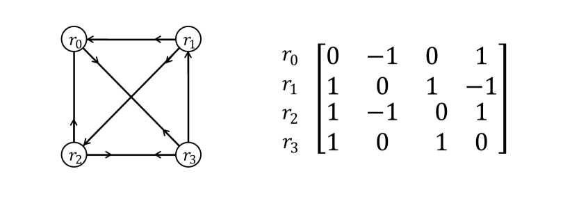
Figure 1. The ancestry relation graph (left) captures all ancestry relations between four splitting rules $\left[r_{0},r_{1},r_{2},r_{3}\right]$. In this graph, nodes represent rules, and arrows represent ancestral relations. An incoming arrow from $r_{j}$ to a node $r_{i}$ indicates that $r_{j}$ is the right-child of $r_{i}$. The absence of an arrow indicates no ancestral relation. An outgoing arrows from $r_{i}$ to a node $r_{j}$ indicates that $r_{j}$ is the left-child of $r_{i}$. The ancestral relation matrix (right) $\boldsymbol{K}$, where the elements $\boldsymbol{K}_{ij}=1$, $\boldsymbol{K}_{ij}=-1$, and $\boldsymbol{K}_{ij}=0$ indicate that $r_{j}$ lies on the positive side, negative side of $r_{i}$, or that there is no ancestry relation between them, respectively.

An important concept that we introduce is rule feasibility: this recognizes the fact that the decision tree model not only divides the ambient space into two regions but also constrains the space in which new splitting rules apply. If a new splitting rule applies only within the subspace defined by its ancestor, we refer to this rule as a feasible rule.

Feasibility essentially establishes an ancestry relation between splitting rules, which must satisfy transitivity. Specifically, if a splitting rule applies to the subspaces defined by its ancestor, it must also apply to the subspace defined by its ancestor’s ancestor rules. We can formalize this ancestry relation with the following definition.

Definition 2.1.

Ancestry relations. Given a list of $K$ rules $\mathit{rs}=\left[r_{1},r_{2},\ldots r_{K}\right]$, the ancestry relation between two hyperplanes is denoted by two arrows $\searrow$ and $\swarrow$. Define $r_{i}\swarrow r_{j}$ if $r_{j}$ is in the left branch of $r_{i}$, and $r_{i}\searrow r_{j}$ if $r_{j}$ is in the right branch of $r_{i}$, and $r_{i}\left(\swarrow\vee\searrow\right)r_{j}$ if $r_{j}$ is in the left or right branch of $r_{i}$.

The notation $\searrow$ and $\swarrow$ must be read from left to right because $h_{i}\swarrow h_{j}$ and $h_{i}\searrow h_{j}$ do not imply $h_{j}\searrow h_{i}$ and $h_{j}\swarrow h_{i}$, unless $h_{i}$ and $h_{j}$ are mutual ancestors of each other. In other words, $\searrow$ and $\swarrow$ are not commutative relations.

These ancestry relations can be characterized as homogeneous binary relations. Relations and graphs are closely related, and homogeneous binary relations over a set can be represented as directed graphs (Schmidt and Ströhlein, 2012). Therefore, the ancestry relations between hyperplanes can be encoded as a complete graph, where the branch nodes (hyperplanes) are the nodes in the graph, and the ancestry relations $\searrow$ and $\swarrow$ are represented as incoming and outgoing arrows in the graph. Note that the adjacent arrows to each node correspond to the ancestry relations. We refer to it as the ancestry relation graph. The reason this graph is complete is that every hyperplane is related to any other hyperplane in some way, either through an ancestry relation or by being unrelated. The left panel in Figure 1 illustrates the corresponding complete graph for a given set of splitting rules, defined by hyperplanes, as shown in Figure 3.

Moreover, binary relations can also be characterized as Boolean matrices. However, to encode two binary relations,$\searrow$ and $\swarrow$ in one matrix, the values $1$ and $-1$ are used to distinguish them. We define the ancestry relation matrix as follows.

Definition 2.2.

Ancestry relation matrix. Given a list of $K$ rules $\mathit{rs}=\left[r_{1},r_{2},\ldots r_{K}\right]$, the ancestry relations between any pair of rules can be characterized as a $K\times K$ square matrix $\boldsymbol{K}$, with elements defined as follows:

• $\boldsymbol{K}_{ij}=1$ if $r_{i}\swarrow r_{j}$ (i.e.,$r_{j}$ is in the left subtree of $r_{i}$),

• $\boldsymbol{K}_{ij}=-1$ if $r_{i}\searrow r_{j}$ (i.e.,$r_{j}$ is in the right subtree of $r_{i}$),

• $\boldsymbol{K}_{ij}=0$ if $r_{i}\overline{\left(\swarrow\vee\searrow\right)}r_{j}$, where $\overline{R}$ represent the complement relation of $R$. According to De Morgan’s law $r_{i}\overline{\left(\swarrow\vee\searrow\right)}r_{j}=\left(r_{i}\overline{\swarrow}r_{j}\right)\wedge\left(r_{i}\overline{\searrow}r_{j}\right)$. In other words, $\boldsymbol{K}_{ij}=0$ if and only if $h_{j}$ is not a branch node in both the left and right subtree of $h_{i}$ and $\boldsymbol{K}_{ij}\neq 0$, $i\neq j$, if $r_{i}$ is the ancestor of $r_{j}$.

We are now ready to formalize the axioms of the decision tree.

Axiom 1.

Axioms for proper decision trees. We call a decision tree that satisfies the following axioms, a proper decision tree:

1. Each branch node is defined by a single splitting rule $r:\mathcal{R}$, and each splitting rule subdivides the ambient space into two disjoint and connected subspaces, $r^{+}$ and $r^{-}$,

2. Each leaf $L$ is defined by the intersection of subspaces $\bigcap_{p\in P_{L}}r_{p}^{\pm}$ for all the splitting rules $\left\{r_{p}\mid p\in P_{L}\right\}$ in the path $P_{L}$ from the root to leaf $L$. The connected region (subspace) defined by $\bigcap_{p\in P_{L}}r_{p}^{\pm}$ is referred to as the decision region,

3. The ancestry relation between any pair of splitting rules $r_{i}\left(\swarrow\vee\searrow\right)r_{j}$ is transitive; in other words, if $r_{i}\left(\swarrow\vee\searrow\right)r_{j}$ and $r_{j}\left(\swarrow\vee\searrow\right)r_{k}$ then $r_{i}\left(\swarrow\vee\searrow\right)r_{k}$,

4. For any pair of splitting rules $r_{i}$ and $r_{j}$, only one of the following three cases is true: $r_{i}\swarrow r_{j}$, $r_{i}\searrow r_{j}$, and $r_{i}\overline{\left(\swarrow\vee\searrow\right)}r_{j}$; additionally, $r_{i}\overline{\left(\swarrow\vee\searrow\right)}r_{i}$ is always true; in other words, $\boldsymbol{K}_{ij}\in\left\{1,0,-1\right\}$, and $\boldsymbol{K}_{ii}=0$, $\forall i,j\in\mathcal{K}$.

Although the ancestry relation satisfies transitivity, it is not a preorder, as it fails to satisfy the reflexive property due to Axiom 4—no rule can be the ancestor of itself in a decision tree. For example, a decision tree with three splitting rules ($K=3$) is rendered as

These axioms encompass a wide range of decision trees, including decision tree models in machine learning, where splitting rules can be axis-parallel hyperplanes or hypersurfaces, as well as binary space partition trees (Tóth, 2005; Motwani and Raghavan, 1996) and $K$-D trees (Bentley, 1975) in computational geometry.

In this study, we focus exclusively on the ODT problem for such proper decision trees. There is potential to extend this framework by modifying or introducing additional axioms to those given above, such as those for the axis-parallel decision tree problem over binary feature data. For this problem, Axiom 4 no longer holds but we can modify it to permit $r_{i}\swarrow r_{j}$ and $r_{i}\searrow r_{j}$ to hold simultaneously for any pair of splitting rules.

2.1.2. When can decision trees be characterized by $K$-permutations?

Figure 2. A decision tree with three splitting rules, corresponds to 3-permutation $\left[r_{1},r_{2},r_{3}\right]$.

The formalization of proper decision trees enables the analysis of their algorithmic and combinatorial properties. One of the most important combinatorial properties discussed in this paper is that any proper decision tree can be uniquely characterized as a $K$-permutation through a level-order traversal of the tree.

Tree traversal refers to the process of visiting or accessing each node of the tree exactly once in a specific order. Level-order traversal visits all nodes at the same level before moving on to the next level. The main idea of level-order traversal is to visit all nodes at higher levels before accessing any nodes at lower levels, thereby establishing a hierarchy of nodes between levels. For example, the level-order traversal for the binary tree in Figure 2 has two possible corresponding $3$-permutations, $\left[r_{1},r_{2},r_{3}\right]$ or $\left[r_{1},r_{3},r_{2}\right]$. If we fix a traversal order such that the left subtree is visited before the right subtree, only one arrangement of rules can exist. Based on the axioms of the proper decision tree, we can state the following theorem about the level-order traversal of a proper decision tree.

Theorem 2.3.

Given a level-order traversal of a decision tree $\left[\ldots,r_{i},\ldots,r_{j},\ldots,r_{k},\ldots\right]$, if $r_{j}$ precedes $r_{k}$ in the traversal, and $r_{i}$ is the ancestor of $r_{j}$ and $r_{k}$, then either:

1. $r_{j}$ and $r_{k}$ are at the same level, or

2. $r_{k}$ is a descendant of $r_{j}$.

Only one of the two cases can occur. If the first case holds, they are the left or right children of another node, and their positions cannot be exchanged.

Proof.

We prove this by contradiction. Assume, by contradiction, $r_{j}$ is in the same level as $r_{k}$ and $r_{k}$ can be a descendant of $r_{j}$. Suppose we have a pair of rules $r_{k}$ and $r_{j}$, where $r_{j}$ precedes $r_{k}$ in the level-order traversal.

Case 1: Assume $r_{j}$ and $r_{k}$ are at the same level, we prove that $r_{k}$ cannot be the descendant of $r_{j}$. Because of Axiom 3, if $r_{j}$ is in the same level of $r_{k}$, then $r_{j}$ and $r_{k}$ are generated from different branches of some ancestor $r_{i}$, which means that they lie in two disjoint regions defined by $r_{i}$. If $r_{k}$ is the descendant of $r_{j}$ then it is also a left-descendant of $r_{i}$ due to associativity. According to Axiom 4, either $r_{j}$ is a left child of $r_{i}$ or right children of $r_{i}$ it can not be both. This leads to a contradiction, as it would imply $r_{k}$ belongs to both disjoint subregions defined by $r_{i}$.

Case 2: Assume $r_{k}$ is a descendant of $r_{j}$, we prove that $r_{j}$ and $r_{k}$ cannot be at the same level. By the transitivity of the ancestry relation, both $r_{k}$ and $r_{j}$ are descendants of the parent node (immediate ancestor) of $r_{j}$, which we call $r_{i}$. Since, $r_{k}$ cannot be both the right- and left-child of $r_{i}$ at the same time, as it must either be the left-child or right-child according to Axiom 4. So $r_{k}$ and $r_{j}$ can not be in the same level if $r_{k}$ is a descendant of $r_{j}$.

Thus, if $r_{j}$ precedes $r_{k}$ in the level-order traversal, this either places them at the same level or establishes an ancestor-descendant relationship between them, but not both. ∎

An immediate consequence of the above theorem is that any $K$-permutation of rules corresponds to the level-order traversal of at most one proper decision tree. The ordering between any two adjacent rules corresponds to only one structure: either they are on the same level, or one is the ancestor of the other. For instance, in Figure 2, if $r_{2}$ and $r_{3}$ are in the same level and $r_{2}$ is the left-child of $r_{1}$, then $r_{3}$ cannot be the child of $r_{2}$, because it cannot be the left-child of $r_{1}$. Hence, only a proper decision tree corresponds to the permutation $\left[r_{1},r_{2},r_{3}\right]$. Therefore, once a proper decision tree is given, we can obtain its $K$-permutation representation easily by using a level-order traversal.

Moreover, the one-to-one correspondence between valid $K$-permutations and proper decision trees implies that the number of $K$-permutations is strictly greater than the number of possible proper decision trees. For instance, if there is only one proper decision tree which corresponds to $K$-permutation $\left[r_{1},r_{3},r_{2}\right]$, then all other $K$-permutations of the set $\left\{r_{1},r_{2},r_{3}\right\}$, are invalid.

Corollary 2.4.

A decision tree consisting of $K$ splitting rules corresponds to a unique $K$-permutation permutation if and only if it is proper. In other words, there exist an injetive mapping from proper decision trees and valid $K$-permtuations.

Proof.

Sufficiency: If a decision tree is proper, its level-order traversal yields a unique valid $K$-permutation by level-order traversal, then it implies it is a proper decision tree

Part 1: Existence of mapping.

Because the level-order traversal algorithm is deterministic and the tree’s structure is fixed (each branch node has a fixed position, left or right child of its parent), thus any binary tree can be transformed into a $K$-permurations, by a level-order traversal.

Part 2: The mapping is injective.

To prove injectivity, we show that distinct proper decision trees $T_{1}\neq T_{2}$ produce distinct permutations $\sigma_{1}\neq\sigma_{2}$. Given two different proper decision trees $T_{1}$ and $T_{2}$, constructed by using rules $\mathit{rs}_{K}=\left\{r_{1},r_{2},\ldots,r_{K}\right\}$. Let $\sigma_{1}$ and $\sigma_{2}$ be their level-order traversals. Assume, for contradiction, that $\sigma_{1}=\sigma_{2}=\sigma=\left[r_{j_{1}},\ldots,r_{j_{K}}\right]$. Since $T_{1}\neq T_{2}$, they differ in some structural property (e.g., $r_{i}$’s parent, sibling order, or level, for any $r_{i}\in\mathit{rs}_{K}$). We examine three cases, showing each alters $\sigma$ :

1. Different sibling order: assume in $T_{1}$, $r_{2}\swarrow r_{3}$ (left child), but in $T_{2}$, $r_{3}\swarrow r_{2}$. In $T_{1}$, $\sigma$ might be $\left[r_{1},\ldots,r_{2},r_{3}\ldots\right]$, and in $T_{1}$, $\sigma$ might be $\left[r_{1},\ldots,r_{2},r_{3}\ldots\right]$, this contradicts $\sigma_{1}=\sigma_{2}$ as sibling order is fixed by Theorem 2.3.

2. Different levels: Suppose in $T_{1}$, $r_{2}$ is a child of $r_{1}$, but in $T_{2}$, $r_{2}$ is a grandchild. Assume $r_{3}$ is the child of $r_{1}$ and father the of $r_{2}$ in $T_{2}$, then we have $\sigma_{1}=\left[r_{1},\ldots,r_{2}\ldots\right]$, $\sigma_{1}=\left[r_{1},\ldots r_{3}\ldots,r_{2}\ldots\right]$. we show that $r_{3}$ can not precedes $r_{2}$ in $\sigma_{1}$. If $r_{3}$ precedes $r_{2}$ in $\sigma_{1}$, then $r_{3}$ is in the same level of $r_{1}$, so $r_{3}$ and $r_{1}$ they are in different branches of another nodes. So $r_{3}$ cannot be the children of $r_{1}$ because of the Theorem 2.3.

3. Different parents: Suppose $r_{1}$’s parent is $r_{2}$ in $T_{1}$ but $r_{3}$ in $T_{2}$. Assume $\sigma_{1}=\sigma_{2}=\sigma=\left[\ldots r_{2},\ldots r_{3}\ldots,r_{1}\ldots\right]$, because $r_{2}$ precedes $r_{3}$ in $\sigma$, so in $T_{1}$, $r_{3}$ must be a node in the same level with $r_{2}$. In $T_{2}$, it can have two possible situations: (1) $r_{2}$ be the ancestor of $r_{3}$; (2) $r_{2}$ is in the same level of $r_{3}$’s ancestor. However, as Theorem 2.3 explained $T_{2}$ cannot coexist with $T_{1}$, because $r_{2}$ and $r_{3}$ (and $r_{2}$ with $r_{3}$’s ancestor in the second case) must be the descendants of another node, if this node changes in $T_{1}$ and $T_{2}$, it results in different permutations anyway.

Thus $\sigma_{1}\neq\sigma_{2}$, we have a contradiction, and the mapping is injective.

Necessity: The mapping from decision trees to $K$-permutations is not injective if the trees are non-proper. Specifically, distinct non-proper decision trees can correspond to identical permutations, rendering the mapping non-unique and thus non-injective.

Consider a permutation $\left[\ldots,r_{i},\ldots,r_{j},\ldots,r_{k},\ldots\right]$. In the absence of Axioms 3 and 4, the structure of the tree is not sufficiently constrained: $r_{j}$ and $r_{k}$ may reside at the same level, or $r_{j}$ is the ancestor of $r_{k}$, within the same permutation. Consequently, this permutation can be realized by at least two distinct non-proper trees $T_{1}$ and $T_{2}$. Since $T_{1}\neq T_{2}$, this gives us an non-injective map. ∎

2.1.3. Incorrect claims in the literature

The study of exact algorithms for ODT problems in machine learning is dominated by the use of ad-hoc branch-and-bound (BnB) methods. Researchers often design algorithms or propose speed-up techniques based on intuition rather than rigorous proof, leading to logical or implementation errors. For instance, in the context of ODT algorithms, the decision tree problem over binary feature data has received the most attention—primarily because its combinatorial complexity is independent of input data size. Several fundamental errors have frequently appeared in the extensive literature on this topic.

The first error, as we note in the introduction, is that the ODT problem over binary feature data does not satisfy the Axiom 4 characterizing proper decision trees. For the decision tree problem over binary feature data, each splitting rule is defined as selecting a feature or not, thus any splitting rule can be both the left-child or right-child of another. So previous research, such as Hu et al. (2019), has wrongly characterized their tree as $K$-permutations, because the decision tree over binary feature data does not satisfy the proper decision tree axioms and hence cannot be characterized by $K$-permutations.

For example, in the decision tree over binary feature data, considering following two trees

Clearly, these two trees are different, but both of them correspond to the same permutation $\left[r_{1},r_{2},r_{3}\right]$ in a level-order traversal. These two trees cannot exist at the same time if they are proper, but can exists in the decision tree over binary feature data. Since the implementation by Hu et al. (2019) differs from their pseudo-code, it remains unclear how their algorithm was actually implemented. Without the required rigorous proof, their algorithm is likely incorrect.

The second error is fundamental: a direct consequence of proper decision tree Axiom 1, is that trees defined by the same set of rules and having the same shape, but organized with different labels, will result in distinct trees. Otherwise, they would be equivalent to unlabeled trees, which correspond to the combinatorial objects counted by Catalan numbers. For instance, consider two trees that share the same topological shape and the same set of splitting rules

These two trees are distinct according to Axiom 1: in the first tree, the decision region defined by the right subtree of $r_{2}$ remains intact after introducing $r_{1}$. Conversely, in the second tree, the decision region defined by the right subtree of $r_{1}$ remains intact after introducing $r_{2}$. Consequently, the first tree creates three decision regions: $r_{2}^{+}\cap r_{1}^{+}$, $r_{2}^{+}\cap r_{1}^{-}$, and $r_{2}^{-}$. The second tree, on the other hand, generates a different set of regions: $r_{2}^{+}\cap r_{1}^{+}$, $r_{2}^{+}\cap r_{1}^{-}$, and $r_{1}^{-}$, which is fundamentally different.

This oversight is a common mistake in the literature studying the ODT problem over binary feature data (Lin et al., 2020; Hu et al., 2020; Aglin et al., 2021, 2020; Nijssen and Fromont, 2007, 2010; Zhang et al., 2023). Many of these reports fail to distinguish trees with the same shape but different labels. For instance, some explicitly count the possible trees using Catalan numbers (Hu et al., 2019), while others employ Catalan number-style recursion (Demirović et al., 2022; Hu et al., 2019; Lin et al., 2020; Zhang et al., 2023; Aglin et al., 2021, 2020; Nijssen and Fromont, 2010).

Finally, another fundamental error found in the literature is the improper application of memoization techniques for decision tree problems, a problem which will be explained in detail in section 3.6.2.

2.2. Datatypes, homomorphisms and map functions

Function composition and partial application

The function composition is denoted by using infix symbol $\circ$:

$$\left(f\circ g\right)\left(a\right)=f\left(g\left(a\right)\right).$$

We will try to use infix binary operators wherever possible to simplify the discussion. A binary operator can be transformed into a unary operator through partial application (also known as sectioning). This technique allows us to fix one argument of the binary operator, effectively creating a unary function that can be applied to subsequent values

$$\oplus_{a}\left(b\right)=a\oplus b=\oplus^{b}\left(a\right),$$

where $\oplus$ is a binary operator, such as $+$ or $\times$ for numerical operations, can be partially applied. If $\oplus:\mathcal{A}\times\mathcal{B}\to\mathcal{C}$, then $\oplus_{a}:\mathcal{B}\to\mathcal{C}$, where $a:\mathcal{A}$ is fixed. Moreover, the variables $a$ and $b$ can be functions, we will see examples shortly when we explain the map function.

Datatypes

There are two binary tree data types used in this paper. The first is the leaf-labeled tree, which is defined as

$$\mathit{BTree}\left(\mathcal{A}\right)=L\mid N\left(\mathit{BTree}\left(\mathcal{A}\right),\mathcal{A},\mathit{BTree}\left(\mathcal{A}\right)\right).$$

This definition states that a binary tree $\mathit{BTree}\left(\mathcal{A}\right)$ is either an unlabeled leaf $L$ or a binary tree $N\left(u,a,v\right):\mathit{BTree}\left(\mathcal{A}\right)$, where $u,v:\mathit{BTree}\left(\mathcal{A}\right)$ are the left and right subtrees, respectively, and $a:\mathcal{A}$ is the root node.

An alternative tree definition, called a moo-tree, is named for its phonetic resemblance to the Chinese word for “tree” (Gibbons, 1991), is a binary tree in which leaf nodes and branch nodes have different types. Formally, it is defined as

$$\mathit{MTree}\left(\mathcal{A},\mathcal{B}\right)=DL\left(\mathcal{B}\right)\mid DN\left(\mathit{MTree}\left(\mathcal{A},\mathcal{B}\right),\mathcal{A},\mathit{MTree}\left(\mathcal{A},\mathcal{B}\right)\right).$$

A decision tree is a special case of the moo-tree datatype, which we can define as $\mathit{DTree}\left(\mathcal{R},\mathcal{D}\right)=\mathit{MTree}\left(\mathcal{R},\mathcal{D}\right)$, i.e. a decision tree is a moo-tree where branch nodes are splitting rules and leaf nodes are subsets of the dataset $\mathcal{D}$.

Homomorphisms and fusion

Homomorphisms are functions that fuse into (or propagate through) type constructors, preserving their structural composition. In functional programming and algebraic approaches to program transformation, homomorphisms enable efficient computation by fusing recursive structures into more compact representations.

For example, given a binary operator $\oplus$ and an identity element $e$, a homomorphism over a list is defined as follows:

$$h \left(\left[\,\right]\right)\>\;\quad=e$$

$$h \left(x\cup y\right)=h\left(x\right)\oplus h\left(y\right).$$

Here, $h$ denotes the homomorphism function, where the identity element maps the empty list, and the operation on the concatenation of two lists ($x\cup y$) is the result of applying the binary operator $\oplus$ to the images of the two lists.

Similarly, given $f$ and $y$, there exists a unique homomorphism $h$, such that, for all $u$, $r$ and $v$, the equations

$$h \left(\mathit{DL}\left(a\right)\right)\,\>\;\;\quad=f\left(a\right)$$

$$h \left(\mathit{DN}\left(u,r,v\right)\right)=g\left(h\left(u\right),r,h\left(v\right)\right),$$

hold. The homomorphism $h$ replaces every occurrence of the constructor $\mathit{DL}$ with the function $f$, and every occurrence of the constructor $\mathit{DN}$ with the function $g$, which is essentially a “relabelling” process. Once a homomorphism is identified, a number of fusion or distributivity laws (Bird and De Moor, 1996; Little et al., 2021) can be applied to reason about the properties of the program.

The map functions

One example of fusion is the map function. Given a list $x$ and a unary function $f$, the map function over the list, denoted $\mathit{mapL}$, can be defined as

$$\mathit{mapL}\left(f,x\right)=\left[f\left(x\right)\mid a\leftarrow x\right].$$

This definition corresponds to a standard list comprehension, meaning that the function $f$ is applied to each element $a$ in $x$. By using sectioning, $\mathit{mapL}$ can be partially applied by defining the unary operator $\mathit{mapL}{}_{f}\left(x\right)=\mathit{mapL}\left(f,x\right)$. Similarly, the map function can be defined over a decision tree as follows

$$\mathit{mapD} \left(f,\mathit{DL}\left(a\right)\right)=\mathit{DL}\left(f\left(a\right)\right)$$

$$\mathit{mapD} \left(f,\mathit{DN}\left(u,r,v\right)\right)=DN\left(\mathit{mapD}\left(f,u\right),r,\mathit{mapD}\left(f,v\right)\right).$$

This applies the function $f$ to every leaf of the tree.

3. A generic dynamic programming algorithm for solving the optimal, proper decision tree problem

3.1. Specifying the optimal proper decision tree problem through $K$-permutations

The goal of the ODT problem is to construct a function $\mathit{odt}:\mathbb{N}\times\left[\mathcal{R}\right]\to\mathit{DTree}\left(\mathcal{R},\mathcal{D}\right)$ that outputs the optimal decision tree with $K$ splitting rules. This can be specified as

(2) $$\mathit{odt}_{K} :\left[\mathcal{R}\right]\to\mathit{DTree}\left(\mathcal{R},\mathcal{D}\right)$$

$$\mathit{odt}_{K} =\mathit{min}_{E}\circ\mathit{genDTKs}_{K}.$$

The function $\mathit{genDTKs}_{K}$, short for “generate decision trees with $K$ splitting rules”, generates all possible decision trees of size $K\geq 1$ from a given input of splitting rules $\mathit{rs}:\left[r_{1},r_{2},\ldots r_{M}\right]$, where $M\geq K$. The function $\mathit{min}:\mathit{DTree}\left(\mathcal{R},\mathcal{D}\right)\to\mathbb{R}\to\left[\mathit{DTree}\left(\mathcal{R},\mathcal{D}\right)\right]\to\mathbb{R}$ selects an optimal decision tree from a (assume, non-empty) list of candidates based on the objective value calculated by $E:\mathit{DTree}\left(\mathcal{R},\mathcal{D}\right)\to\mathbb{R}$ (defined in subsection 3.6), which is given by

(3) $$\mathit{min}_{E} \left(\left[a\right]\right)=a$$

$$\mathit{min}_{E} \left(a:\mathit{as}\right)=\mathit{smaller}_{E}\left(a,min_{E}\left(\mathit{as}\right)\right),$$

where $:$ denotes list construction (or prepending) so that $a:as$ prepends the element $a$ to the front of the list $as$. The function $\mathit{smaller}_{E}$ is defined as follows

(4) $$\mathit{smaller}_{E}\left(a,b\right)=\begin{cases}a,&\text{if $E\left(a\right)\leq E\left(b\right)$}\\ b,&\text{otherwise}.\end{cases}$$

The above specification of $\mathit{odt}$ (2) is essentially a brute-force program, i.e. it exhaustively generates all possible configurations and then selects the best one. However, this specification is typically inefficient, as the number of trees generated by $\mathit{genDTKs}$ usually grows exponentially with the size of $\mathit{\mathit{rs}}$. Generating all possible trees and then comparing their costs one by one is not an efficient strategy.

To make this program practical, two major aspects must be considered to improve efficiency. Firstly, we need to define an efficient version of $\mathit{genDTKs}$; secondly, when the generator $\mathit{genDTKs}$ is defined as a recursive program, it is often possible to fuse $\mathit{min}_{E}$ and $\mathit{genDTKs}$ into a single function. This fusion allows for significant computational savings, as partial configurations that are non-optimal can be eliminated without fully generating them. Program fusion such as this is a powerful and general technique. In fact, dynamic programming, branch-and-bound, and greedy algorithms can all be derived through this kind of program fusion (De Moor, 1994; Bird and De Moor, 1996).

As discussed, proper decision trees can be characterized as $K$-permutations of rules. Thus one possible definition of the $\mathit{genDTKs}$ function is

(5) $$\mathit{genDTKs}_{K} :\left[\mathcal{R}\right]\to\left[\left[\mathcal{R}\right]\right]$$

$$\mathit{genDTKs}_{K} =\mathit{filter}_{p}\circ\mathit{kperms}_{K}.$$

The program begins by generating all possible $K$-permutations using $\mathit{kperms}_{K}$, and then filters out, using $\mathit{filter}_{p}$, those that cannot be used to construct proper decision trees. This two-step process ensures that only valid permutations—those that satisfy the predicate $p$, i.e. meet the structural and combinatorial requirements of proper decision trees—are retained in further computations. We can substitute $\mathit{genDTKs}_{K}$ into the definition of $\mathit{odt}_{K}$, and thus we have

(6) $$\mathit{odt}{}_{K} :\left[\mathcal{R}\right]\to\left[\left[\mathcal{R}\right]\right]$$

$$\mathit{odt}{}_{K} =\mathit{min}{}_{E}\circ\mathit{filte}r{}_{p}\circ\mathit{kperm}s{}_{K}.$$

As mentioned, numerous algorithms can generate permutations efficiently (Sedgewick, 1977). One possible definition of a $K$-permutation generator is defined through a $K$-combination generator—$K$-permutations are simply all possible rearrangements (permutations) of each $K$-combination. In other words, we can define $\mathit{kperms}_{K}$ by the following

(7) $$\mathit{kperms}{}_{K}=\mathit{concatMapL}{}_{perms}\circ\mathit{kcombs}_{K},$$

where $\mathit{perms}:\left[\mathcal{A}\right]\to\left[\left[\mathcal{A}\right]\right]$ generates all possible permutations of a given list, and $\mathit{concatMapL}=\mathit{concat}\circ\mathit{mapL}$, the flatten operation $\mathit{concat}:\left[\left[\mathcal{A}\right]\right]\to\left[\mathcal{A}\right]$ collapses the inner lists into a single list. Thus, by substituting the definition of $\mathit{kperms}{}_{K}$ into $\mathit{odt}_{K}$, we obtain,

(8) $$\mathit{odt}{}_{K} :\left[\mathcal{R}\right]\to\left[\left[\mathcal{R}\right]\right]$$

$$\mathit{odt}{}_{K} =\mathit{mi}n{}_{E}\circ\mathit{filter}{}_{p}\circ\mathit{concat}\circ\mathit{mapL}{}_{perms}\circ\mathit{kcombs}{}_{K},$$

and $\mathit{genDTKs}_{K}=\mathit{filter}{}_{p}\circ\mathit{concat}\circ\mathit{mapL}{}_{perms}\circ\mathit{kcombs}{}_{K}$. Since $\mathit{kcombs}{}_{K}$ produces only $\left(\begin{array}[]{c}M\\ K\end{array}\right)=O\left(M^{K}\right)$ $K$-combinations, and $K$-permutations are all possible permutations of each $K$-combinations, thus we have $\left|\mathit{kperms}_{K}\right|=K!\times\left(\begin{array}[]{c}M\\ K\end{array}\right)=O\left(M^{K}\right)$. This already gives a polynomial-time algorithm for solving the ODT problem (assuming that the predicate $p$ has polynomial complexity and $\mathit{min}_{E}$ is linear in the candidate list size).

3.1.1. The redundancy of $K$-permutations

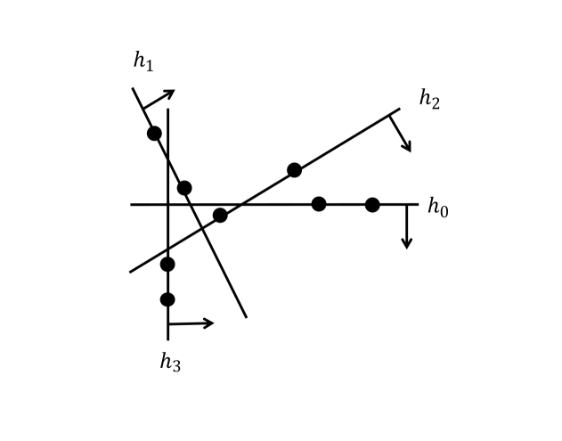
Figure 3. Four hyperplanes in $\mathbb{R}^{2}$. The black circles represent data points used to define these hyperplanes, and the black arrows indicate the direction of the hyperplanes.

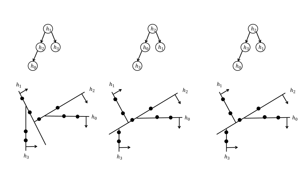
Figure 4. Three possible decision trees and their corresponding partitions of space in $\mathbb{R}^{2}$ for the four hyperplanes depicted in Figure 3. The three decision trees above represent all possible decision trees, the three figures below describe the partition of space $\mathbb{R}^{2}$ resulting from the corresponding decision tree.

The definition above, based on $K$-permutations, remains unsatisfactory. The number of proper decision trees for a given set of rules is typically much smaller than the total number of permutations, and determining whether a permutation is feasible is often non-trivial. To quantify the redundancy in generated permutations and the complexity of feasibility test, we examine a specific case—the hyperplane decision tree problem—where splitting rules are defined by hyperplanes.

He and Little (2023) showed that hyperplanes in $\mathbb{R}^{D}$ can be constructed using $D$-combinations of data points. Consequently, within a decision region, hyperplanes can only be generated from the data points contained in the decision region defined by their ancestors. This implies that the feasibility test $p$ in the hyperplane decision tree problem must ensure that all data points defining the hyperplanes in a subtree remain within the decision region specified by its ancestors. This requirement imposes a highly restrictive constraint.

To assess the impact of this constraint, we introduce simple probabilistic assumptions. Suppose each hyperplane classifies a data point into the positive or negative class with equal probability, i.e. 1/2 for each class. If a hyperplane can serve as the root of a decision tree, the probability of this occurring is $\left(\frac{1}{2}\right)^{D\times\left(K-1\right)}$, since each hyperplane is defined by $D$-combinations of data points. Furthermore, the probability of constructing a proper decision tree with a chain-like structure (each branch node has at most one child) is given by

$$\left(\frac{1}{2}\right)^{D\times\left(K-1\right)}\times\left(\frac{1}{2}\right)^{D\times\left(K-2\right)}\times\ldots\times\left(\frac{1}{2}\right)^{D}=O\left(\left(\frac{1}{2}\right)^{D\times K^{2}}\right).$$

In subsection 3.6.3, we will show that when a decision tree has a chain-like structure, it exhibits the highest combinatorial complexity. This naive probabilistic assumption provides insight into the rarity of proper decision trees with $K$ splitting rules compared to the total number of $K$-permutations of splitting rules.

For example, the 4-combination of hyperplanes shown in Figure 3 produces only three decision trees, as illustrated in Figure 4, while the total number of possible permutations is $4!$=24. Interestingly, although there are three possible trees, there are only two possible partitions. This suggests an interesting direction for further speeding up the algorithm by eliminating such cases, as our current algorithm cannot remove these duplicate partitions.

Moreover, the feasibility test is a non-trivial operation. For each hyperplane, it must be verified whether the data points used to define it lie within the same region as determined by its ancestor hyperplanes. Testing whether $D$ points are on the same side of a hyperplane requires $O\left(D^{2}\right)$ computations. Given that a decision tree is defined by $K$ hyperplanes, and in the worst case, a hyperplane may have $K$ ancestors, the feasibility test incurs a worst-case time complexity of $O\left(K^{2}D^{2}\right)$.

Therefore, in order to achieve the optimal efficiency, it is essential to design a tree generator that directly generates only proper decision trees, eliminating the need for post-generation filtering, and even better, this generator is amenable to fusion. Next, we will explain the design of such a proper decision tree generator and then demonstrate that the recursive generator is fusable with the $min_{E}$ function.

3.2. A simplified decision tree problem: the decision tree problem with $K$ fixed splitting rules (branch nodes)

In the expanded specification (8), we have obtained

(9) $$\mathit{genDTKs}_{K}=\mathit{filter}{}_{p}\circ\mathit{flatten}\circ\mathit{mapL}{}_{perms}\circ\mathit{kcombs}{}_{K}.$$

This program suggests two potential approaches for fusion. The first approach, as described in the previous section, involves fusing $mapL_{perms}$ with $\mathit{kcomb}s{}_{K}$ to obtain a single $\mathit{kperms}$ function. However, as illustrated above a major drawback of this method is that the number of proper decision trees for a given set of rules is significantly smaller than the total number of permutations.

Alternatively, we can try to fuse the composed function $\mathit{filter}{}_{p}\circ\mathit{concat}\circ\mathit{mapL}{}_{perms}$ by following equational reasoning

$$\mathit{filter}{}_{p}\circ\mathit{concat}\circ\mathit{mapL}{}_{perms}\circ\mathit{kcombs}{}_{K}$$

$$\equiv \mathit{filter}_{p}\circ\mathit{concat}=\mathit{concat}\circ\mathit{mapL}_{\mathit{filter}_{p}}$$ filter fusion laws

$$\mathit{concat}\circ\mathit{mapL}{}_{\mathit{filter}_{p}}\circ\mathit{mapL}{}_{perms}\circ\mathit{kcombs}{}_{K}$$

$$\equiv \mathit{mapL}_{f}\circ\mathit{mapL}_{g}=\mathit{mapL}_{f\circ g}$$ map composition

$$\mathit{concat}\circ\mathit{mapL}{}_{\mathit{filter}_{p}\circ\mathit{perms}}\circ\mathit{kcombs}{}_{K}$$

$$\equiv \mathit{genDTs}=\mathit{filter}_{p}\circ\mathit{perms}$$ define

$$\mathit{concatMapL}{}_{genDTs}\circ\mathit{kcombs}{}_{K},$$

where the laws used in above derivation can all be found in Bird (1987) (since these laws are easy to verify and intuitively obvious, we do not repeat their proofs here).

Now, we can redefine $\mathit{genDTKs}_{K}$ as

(10) $$\mathit{genDTKs}_{K}=\mathit{concatMapL}{}_{genDTs}\circ\mathit{kcombs}{}_{K},$$

where $\mathit{genDTs}=\mathit{filter}_{p}\circ\mathit{perms}$. The function $\mathit{genDTs}$ first generates all permutations of a given $K$-combination that then selects those the satisfy the feasibility test $p$. In other words, $\mathit{genDTs}$ returns all possible valid permutations of a given $K$-combination, and this function is applied to each $K$-combination generated by $\mathit{kcombs}{}_{K}$.

Note that (10) is just a new specification of $\mathit{genDTs}$; we have not yet come up with an efficient definition for it. If we can fuse $\mathit{filter}_{p}\circ\mathit{perms}$ into a single program, this would eliminate the need for a feasibility test, as all decision trees produced by the generator are inherently proper by design. We could then potentially obtain an efficient definition for $\mathit{genDTs}_{K}$ and consequently, an efficient definition for $\mathit{genDTKs}_{K}$ as well. Indeed, one of the main contributions of this paper is to derive an efficient definition for $\mathit{genDTs}$, which will be explored in subsection 3.5.

Assuming for now we have an efficient definition for $\mathit{genDTs}$, the optimal decision tree problem can be reformulated as

(11) $$\mathit{odt}{}_{K} :\left[\mathcal{R}\right]\to\mathit{DTree}\left(\mathcal{R},\mathcal{D}\right)$$

$$\mathit{odt}{}_{K} =\mathit{min}{}_{E}\circ\mathit{concatMapL}{}_{genDTs}\circ\mathit{kcombs}{}_{K}.$$

In this definition, $\mathit{odt}{}_{K}$ receives a list of all possible rules $\mathit{rs}$, where $\left|\mathit{rs}\right|\geq K$ and generates all possible $K$-combinations of them. Then the $\mathit{genDTs}$ function is applied to each $K$-combination of rules generated by $\mathit{kcombs}{}_{K}$. It is important to distinguish $\mathit{genDTs}$ from $\mathit{genDTKs}_{K}$. The latter is parameterized by $K$, whereas $\mathit{genDTs}$ operates on the output of $\mathit{kcombs}{}_{K}$, without being explicitly parameterized by $K$.

Moreover, specification (11) suggests another potential fusion

$$\mathit{min}{}_{E}\circ\mathit{mapL}{}_{genDTs}\circ\mathit{kcombs}{}_{K}$$

$$\equiv \mathit{minlist}_{E}\circ\mathit{concat}=\mathit{min}_{E}\circ\mathit{mapL}_{\mathit{min}_{E}}$$ reduce promotion law

$$\mathit{min}{}_{E}\circ\mathit{mapL}{}_{\mathit{min}_{E}\circ genDTs}\circ\mathit{kcombs}{}_{K}$$

$$\equiv \mathit{sodt}=\mathit{min}_{E}\circ\mathit{genDTs}$$ define

$$\mathit{min}{}_{E}\circ\mathit{mapL}_{\mathit{sodt}}\circ\mathit{kcombs}{}_{K}.$$

Again, the reduce promotion law used in the derivation can be found in Bird (1987). Then, we have following new definition for the optimal decision tree problem,

(12) $$\mathit{odt}{}_{K}^{\prime} :\left[\mathcal{R}\right]\to DTree\left(\mathcal{R},\mathcal{D}\right)$$

$$\mathit{odt}{}_{K}^{\prime} =\mathit{min}{}_{E}\circ\mathit{mapL}{}_{sodt}\circ\mathit{kcombs}{}_{K},$$

where $\mathit{sodt}$ is short for “simplified optimal decision tree problem”, which is defined as

(13) $$\mathit{sodt} :\left[\mathcal{R}\right]\to\mathit{DTree}\left(\mathcal{R},\mathcal{D}\right)$$

$$\mathit{sodt} =\mathit{min}{}_{E}\circ\mathit{genDTs}.$$

The function $\mathit{sodt}\left(\mathit{rs}_{K}\right)$ finds the optimal decision tree with respect to a $K$-combination of the rules $\mathit{rs}_{K}$. Then, if we apply $\mathit{sodt}\left(\mathit{rs}_{K}\right)$ to each $K$-combination of rules ($rs_{K}\in\mathit{kcombs}{}_{K}\left(\mathit{rs}\right)$), we thereby obtain the optimal solution to the ODT problem $\mathit{\mathit{odt}{}_{K}^{\prime}}$.

The function $\mathit{odt}{}_{K}^{\prime}$ is potentially more efficient than $\mathit{odt}{}_{K}$, for two reasons. Firstly, program $\mathit{sodt}$ is defined based on $\mathit{genDTs}$, which directly generates proper decision trees instead of $K$-permutations. As we have discussed, the number of possible $K$-permutations is much larger than the number of proper decision trees. Secondly, for each $K$-combination of $rs$, there is only one optimal decision tree returned by $\mathit{sodt}$. The $\mathit{min}{}_{E}$ function in $\mathit{odt}{}_{K}^{\prime}$ only needs to select the optimal decision tree from the set of optimal decision trees generated by $\mathit{mapL}{}_{sodt}\circ\mathit{kcombs}{}_{K}$, which is significantly smaller than the set of all possible decision trees of size $K$.

Therefore, the focus can be shifted to solving the following problem:

What is the optimal proper decision tree with respect to $K$ fixed splitting rules, where the splitting rules are hyperplanes characterized as combinations of data points? Does there exist a greedy or dynamic programming (DP) solution to this problem?

In other words, we seek an efficient definition for the function $\mathit{genDTs}$, which takes a fixed sequence ($K$-combination) of rules $rs_{K}$ and generates all possible decision trees based on $\mathit{rs}{}_{K}$. Moreover, if we can fuse $\mathit{min}{}_{E}$ with $\mathit{genDTs}$, it could lead to a greedy or dynamic programming solution for $\mathit{sodt}$. The following discussion addresses these two questions.

3.3. An efficient proper decision tree generator

As discussed in the background section, the structure of the decision tree is completely determined by the branch nodes, as the leaf nodes are defined by the intersections of the subspaces for all splitting rules in the path from the root to the leaf.

Therefore, to present a step-by-step derivation for $\mathit{genDTs}$, we first describe the construction of a “partial decision tree generator” $\mathit{genBTs}$, using the $\mathit{BTree}\left(\mathcal{R}\right)$ datatype. Then, we progressively extend the discussion to develop a “complete decision tree generator” by using Gibbons (1996)’s downward accumulation technique, in the next section.

In order to construct a tree generator, there is the need to address an important question: which splitting rules can be the root of the tree? Because of Axiom 3, not every splitting rule can be the ancestor of another, and the root of the tree is the only thing we need to consider, because all splitting rules are the root of some subtrees.

Since the ancestry relation satisfies transitivity, any splitting rules making up the root of the tree must be the ancestor of all its descendants. In other words, given $K$ fixed rules $\mathit{rs}_{K}$, if $r_{i}$ is the root, then $r_{i}\left(\swarrow\vee\searrow\right)r_{j}$, for all $r_{j}\in\mathit{rs}_{K}$ such that $j\neq i$. In the ancestry relation graph, if $r_{i}$ is the root, all edges connected to $r_{i}$ and $r_{j}\in rs_{K}$ for $j\neq i$ must have arrows, either incoming or outgoing. For example, in Figure 1, $r_{0}$ cannot be the root of $\mathit{rs}_{4}=\left[r_{0},r_{1},r_{2},r_{3}\right]$, because the head is closer to $r_{0}$ in the edge between $r_{0}$ to $r_{2}$, which does not contain an arrow. More simply, since $\boldsymbol{K}_{ij}\neq 0$, if $h_{i}$ can be the ancestor of $r_{j}$, then a rule $r_{i}$ can be the root if and only if $\boldsymbol{K}_{ij}\neq 0$ for all $r_{j}\in\mathit{rs}_{K}$. Therefore, a $\mathit{splits}$ function can be constructed that identifies which splitting rules, within a given list of rules $rs$, are viable candidates to become the root of a proper decision tree

$$splits :\left[\mathcal{R}\right]\to\left[\left(\left[\mathcal{R}\right],\mathcal{R},\left[\mathcal{R}\right]\right)\right]$$

$$splits \left(\mathit{rs}\right)=\left[\left(\mathit{rs}^{+},r_{i},\mathit{rs}^{-}\right)\mid r_{i}\leftarrow rs,\mathit{all}\left(r_{i},\mathit{rs}\right)=\mathit{True}\right],$$

where $rs^{+}=\left[r_{j}\mid r_{j}\leftarrow rs,K_{ij}=1\right]$, $rs^{+}=\left[r_{j}\mid r_{j}\leftarrow rs,K_{ij}=-1\right]$ and $\mathit{all}\left(r_{i},rs\right)$ returns true if all rules $r_{j}$ in $rs$ satisfy $K_{ij}\neq 0$ for $i\neq j$, and false otherwise.

The $\mathit{splits}$ function divides a list of rules $rs$ into a triple—the rules classified into the left subtree $rs^{+}$, the root hyperplanes $r$, and the rules classified into the right subtree $rs^{-}$. A similar $\mathit{splits}$ function is also used ambiguously in studying the ODT problem over binary feature data, as explored in several papers (Lin et al., 2020; Zhang et al., 2023; Hu et al., 2019). However, none of these studies explicitly define this splitting function, and it remains obscure how the algorithm works in actual implementation. Only Demirović et al. (2022) defines this function explicitly in a recursion but it is incorrect for the ODT problem over binary feature data because they have employed a Catalan number-style recursion.

With the help of the $\mathit{splits}$ function, which makes sure only feasible splitting rules—those that can serve as the root of a tree or subtree—are selected as the root—we can define an efficient decision tree generator as follows

$$\mathit{genBTs} :\left[\mathcal{R}\right]\to\left[\mathit{BTree}\left(\mathcal{R}\right)\right]$$

$$\mathit{genBTs} \left(\left[\;\right]\right)=\left[L\right]$$

$$\mathit{genBTs} \left(\left[r\right]\right)=\left[N\left(L,r,L\right)\right]$$

$$\mathit{genBTs} \left(\mathit{rs}\right)=\left[N\left(u,r_{i},v\right)\mid\left(rs^{+},r_{i},rs^{-}\right)\leftarrow\mathit{splits}\left(\mathit{rs}\right),u\leftarrow\mathit{genBTs}\left(\mathit{rs}^{+}\right),v\leftarrow\mathit{genBTs}\left(\mathit{rs}^{-}\right)\right].$$

This $\mathit{genBTs}$ generator function recursively constructs larger proper decision trees $N\left(u,r_{i},v\right)$ from smaller proper decision trees $\mathit{genBTs}\left(\mathit{rs}^{+}\right)$ and $\mathit{genBTs}\left(\mathit{rs}^{-}\right)$, the $\mathit{splits}$ funnction ensuring that only feasible splitting rules can become the root of a subtree during recursion. Note that the definition of $\mathit{\mathit{genBTs}}$ (and $\mathit{\mathit{genDTs}}$ as well) does not require the input sequence $rs$ to have a fixed size, as it can process input sequences of arbitrary length. However, when used within the $\mathit{sodt}$ function, it must be constrained to ensure that the generated tree has a fixed size $K$.

The complexity of $\mathit{genBTs}$ depends on the number of possible proper decision trees. Since this number is determined by the distribution of the data, it is challenging to analyze the complexity precisely. However, we will provide a worst-case combinatorial complexity analysis in a later discussion, which shows that the algorithm has a complexity of $O\left(K!\times N\right)$ in the worst case, where $K$ is the number of branch nodes.

3.4. Downwards accumulation for proper decision trees

We are now half way towards our goal. The $\mathit{genBTs}$ function provides an efficient way of generating the structure of the decision tree, namely binary tree representations of a decision tree. However, this is just a partial decision tree generator. Since a decision tree is not a binary tree, we need to figure out how to “pass information down the tree” from the root towards the leaves during the recursive construction of the tree. In other words, we need to accumulate all the information for each path of the tree from the root to each leaf.

In this section we introduce a technique called downwards accumulation Gibbons (1991), which will helps us to construct the “complete decision tree generator.” Accumulations are higher-order operations on structured objects that leave the shape of an object unchanged, but replace every element of that object with some accumulated information about other elements. For instance, the prefix sums (with binary operator $\oplus$) over a list are an example of accumulation over list $\left[a_{1},a_{2},\ldots a_{n}\right]$,

$$\left[a_{1},a_{1}\oplus a_{2},\ldots,a_{1}\oplus a_{2}\oplus\ldots\oplus a_{n}\right].$$

Downward accumulation over binary trees is similar to list accumulation, as it replaces every element of a tree with some function of that element’s ancestors. For example, given a tree

applying downwards accumulation with binary operator $\oplus$ to the above tree results in

The information in each leaf is determined by the path from the root to that leaf. Therefore, Gibbons (1991)’s downward accumulation method can be adopted for constructing the decision tree generator.

To formalize downward accumulation, as usual, we first need to define a path generator and a path datatype. The ancestry relation can be viewed as a path of length one, thus we can abstract $\swarrow$ and $\searrow$ as constructors of the datatype. We define the path datatype recursively as

$$\mathcal{P}\left(\mathcal{A}\right)=S\left(\mathcal{A}\right)\mid\mathcal{P}\left(\mathcal{A}\right)\swarrow\mathcal{P}\left(\mathcal{A}\right)\mid\mathcal{P}\left(\mathcal{A}\right)\searrow\mathcal{P}\left(\mathcal{A}\right),$$

in words, a path is either a single node $S\left(\mathcal{A}\right)$, or two paths connected by $\swarrow$ or $\searrow$.

The path reduction (also known as a path homomorphism), applies to a path and reduces it to a single value:

$$\mathit{pathRed} ::\left(\mathcal{A}\to\mathcal{B}\right)\times\left(\mathcal{A}\to\mathcal{B}\to\mathcal{B}\right)\times\left(\mathcal{A}\to\mathcal{B}\to\mathcal{B}\right)\times\mathcal{P}\left(\mathcal{A}\right)\to\mathcal{B}$$

$$\mathit{pathRed} \left(f,\oplus,\otimes,S\left(\mathit{xs}\right)\right)=f\left(\mathit{xs}\right)$$

$$\mathit{pathRed} \left(f,\oplus,\otimes,p\swarrow q\right)=\mathit{pathRed}\left(\oplus^{\mathit{pathRed}\left(f,\oplus,\otimes,q\right)},\oplus,\otimes,p\right)$$

$$\mathit{pathRed} \left(f,\oplus,\otimes,p\searrow q\right)=\mathit{pathRed}\left(\otimes^{\mathit{pathRed}\left(f,\oplus,\otimes,q\right)},\oplus,\otimes,p\right).$$

The next step toward defining downward accumulation requires a function that generates all possible paths of a tree. For this purpose, Gibbons (1996) introduced a definition of paths over a binary tree, which replaces each node with the path from the root to that node. However, the accumulation required for the decision tree problem differs from the classical formulation. In Gibbons (1996)’s downward accumulation algorithm, information is propagated to every node, treating both branch and leaf nodes uniformly. By contrast, the decision tree problem requires passing information only to the leaf nodes, leaving the branch nodes unchanged.

Analogous to Gibbons (1996)’s definition of $\mathit{paths}$ for binary tree datatypes, we can alternatively define the path generator as

$$\mathit{paths} :\left(\mathcal{B}\to\mathcal{A}\right)\times\left(\mathcal{B}\to\mathcal{A}\right)\times\mathit{DTree}\left(\mathcal{B},\mathcal{A}\right)\to\mathit{DTree}\left(\mathcal{B},\mathcal{P}\left(\mathcal{A}\right)\right)$$

$$\mathit{paths} \left(f,g,\mathit{DL}\left(\mathit{xs}\right)\right)=\mathit{DL}\left(S\left(\mathit{xs}\right)\right)$$

$$\mathit{paths} \left(f,g,\mathit{DN}\left(u,r,v\right)\right)=\mathit{DN}\left(\mathit{mapD}{}_{\swarrow_{S\left(f\left(r\right)\right)}}\left(\mathit{paths}\left(f,g,u\right)\right),S\left(r\right),\mathit{mapD}{}_{\searrow_{S\left(g\left(r\right)\right)}}\left(\mathit{paths}\left(f,g,v\right)\right)\right),$$

where $\mathcal{P}$ receives only one type $\mathcal{A}$, two functions $f$ and $g$ are used to transform $r:\mathcal{B}$ into type $\mathcal{A}$ , while also distinguishing between “left turn” ($\swarrow$) and “right turn” ($\searrow$).

To see how this works, consider the decision tree $T$ given below, where for simplicity, the singleton path constructor $S\left(\;\right)$ is left implicit, and we denote the leaf value using symbol $\diamond:S\left(\mathcal{A}\right)$:

Running $paths$ on decision tree $T$, we obtain

Here, only the leaf nodes are replaced with the path from the root to the ancestors, while the structure and branch nodes of the tree remain unchanged. Our required downward accumulation over proper decision tree datatypes, passes all information to the leaf nodes, leaving the splitting rules (branch nodes) unchanged. This can be formally defined as

$$\mathit{dacc}_{h,f,g,\oplus,\otimes} =\mathit{mapD}{}_{\mathit{pathRed}{}_{h,\oplus,\otimes}}\circ\mathit{paths}_{f,g}.$$

Every downward accumulation has the following property

$$\mathit{mapD}{}_{\mathit{pathRed}{}_{h,\oplus,\otimes}} \left(\mathit{paths}_{f,g}\left(\mathit{DN}\left(u,r,v\right)\right)\right)=$$

$$\mathit{DN}\bigg{(}\mathit{mapD}{}_{\oplus_{f\left(r\right)}}\left(\mathit{mapD}{}_{\mathit{pathRed}{}_{h,\oplus,\otimes}}\left(\mathit{paths}_{f,g}\left(u\right)\right)\right),r$$

$$\quad\quad\quad\mathit{mapD}{}_{\otimes_{g\left(r\right)}}\left(\mathit{mapD}{}_{\mathit{pathRed}{}_{h,\oplus,\otimes}}\left(\mathit{paths}_{f,g}\left(v\right)\right)\right)\bigg{)},$$

which can be proved by following equational reasoning

$$\mathit{mapD}{}_{\mathit{pathRed}{}_{h,\oplus,\otimes}}\left(\mathit{paths}_{f,g}\left(\mathit{DN}\left(u,r,v\right)\right)\right)$$

$$\equiv \mathit{paths}$$ definition of

$$\mathit{mapD}{}_{\mathit{pathRed}{}_{h,\oplus,\otimes}}\left(\mathit{DN}\left(\mathit{mapD}_{\swarrow_{S\left(f\left(r\right)\right)}}\left(\mathit{paths}_{f,g}\left(u\right)\right),r,\mathit{mapD}_{\searrow_{S\left(g\left(r\right)\right)}}\left(\mathit{paths}_{f,g}\left(v\right)\right)\right)\right)$$

$$\equiv \mathit{mapD}$$ definition of

$$\mathit{DN}\left(\mathit{mapD}{}_{\mathit{pathRed}{}_{h,\oplus,\otimes}}\left(\mathit{mapD}_{\swarrow_{S\left(f\left(r\right)\right)}}\left(\mathit{paths}_{f,g}\left(u\right)\right)\right),r,\mathit{mapD}{}_{\mathit{pathRed}{}_{h,\oplus,\otimes}}\left(\mathit{mapD}_{\searrow_{S\left(g\left(r\right)\right)}}\left(\mathit{paths}_{f,g}\left(v\right)\right)\right)\right)$$

$$\equiv$$ map composition

$$\mathit{DN}\left(\mathit{mapD}_{\mathit{pathRed}{}_{h,\oplus,\otimes}\circ\swarrow_{S\left(f\left(r\right)\right)}}\left(\mathit{paths}_{f,g}\left(u\right)\right)\right),r,\mathit{mapD}{}_{\mathit{pathRed}{}_{h,\oplus,\otimes}}\left(\mathit{mapD}_{\mathit{pathRed}{}_{h,\oplus,\otimes}\circ\searrow_{S\left(g\left(r\right)\right)}}\left(\mathit{paths}_{f,g}\left(v\right)\right)\right)$$

$$\equiv \mathit{pathRed}$$ definition of

$$\mathit{DN}\left(\mathit{mapD}{}_{\oplus_{f\left(r\right)}\circ\mathit{pathRed}{}_{h,\oplus,\otimes}}\left(\mathit{paths}_{f,g}\left(u\right)\right),r,\mathit{mapD}{}_{\mathit{\otimes_{g\left(r\right)}\circ pathRed}{}_{h,\oplus,\otimes}}\left(\mathit{paths}_{f,g}\left(v\right)\right)\right)$$

$$\equiv$$ map composition

$$\mathit{DN}\left(\mathit{mapD}_{\oplus_{f\left(r\right)}}\left(\mathit{mapD}{}_{\mathit{pathRed}{}_{h,\oplus,\otimes}}\left(\mathit{paths}_{f,g}\left(u\right)\right)\right),r,\mathit{mapD}_{\otimes_{g\left(r\right)}}\left(\mathit{mapD}{}_{\mathit{pathRed}{}_{h,\oplus,\otimes}}\left(\mathit{paths}_{f,g}\left(v\right)\right)\right)\right),$$

then downwards accumulation is both efficient and homomorphic. This homomorphic downward accumulation can be computed in parallel functional time proportional to the product of the depth of the tree and the time taken by the individual operations (Gibbons, 1996), and thus is amenable to fusion.

3.5. An efficient definition of a proper decision tree generator

In section 3.3, we described the construction of a decision tree generator based on the binary tree data type. However, the $\mathit{\mathit{genBTs}}$ function generates only the structure of the decision tree, which contains information solely about the branch nodes. While this structure is sufficient for evaluating the tree, constructing a complete decision tree—one that incorporates both branch nodes and leaf nodes—is essential for improving the algorithm’s efficiency.

Before we moving towards deriving a complete decision tree generator, we need to generalize $\mathit{genBTs}$ to define it over the $\mathit{DTree}$ datatype

$$\mathit{genBTs}^{\prime} :\left[\mathcal{R}\right]\times\mathcal{D}\to\left[\mathit{DTree}\left(\mathcal{R},\mathcal{D}\right)\right]$$

$$\mathit{genBTs}^{\prime} \left(\left[\;\right],\mathit{xs}\right)=\left[\mathit{DL}\left(\mathit{xs}\right)\right]$$

$$\mathit{genBTs}^{\prime} \left(\left[r\right],\mathit{xs}\right)=\left[\mathit{DN}\left(\mathit{DL}\left(\mathit{xs}\right),r,\mathit{DL}\left(\mathit{xs}\right)\right)\right]$$

$$\mathit{genBTs}^{\prime} \left(\mathit{rs},\mathit{xs}\right)=\left[\mathit{DN}\left(u,r_{i},v\right)\mid\left(\mathit{rs}{}^{+},r_{i},\mathit{rs}{}^{-}\right)\leftarrow\mathit{splits}\left(\mathit{rs}\right),u\leftarrow\mathit{genBTs}^{\prime}\left(\mathit{rs}{}^{+},\mathit{xs}\right),v\leftarrow\mathit{genBTs}^{\prime}\left(\mathit{rs}{}^{-},\mathit{xs}\right)\right].$$

The difference between complete and partial decision tree generator lies in the fact that the complete one contains accumulated information in leaves and the partial one has no information, just the leaf label $L$. This reasoning allows us to define the complete decision tree generator $\mathit{genDTs}$ based on the partial $\mathit{genBTs}^{\prime}$ as follows:

$$\mathit{genDTs}\left(\mathit{rs},\mathit{xs}\right)=\mathit{mapL}_{\mathit{dacc}_{\mathit{id},\mathit{sl},\mathit{sr},\cap,\cap}}\left(\mathit{genBTs}^{\prime}\left(\mathit{rs},\mathit{xs}\right)\right),$$

where $\mathit{sl}$ and $\mathit{sr}$ are short for “split left”, and “split right”, respectively, defined as $\mathit{sl}\left(r\right)=r^{+}$ and $\mathit{sr}\left(r\right)=r^{-}$. We can derive $\mathit{genDTs}$ by the following equational reasoning

$$\mathit{mapL}_{\mathit{dacc}_{\mathit{id},\mathit{sl},\mathit{sr},\cap,\cap}}\left(\mathit{genBTs}^{\prime}\left(\mathit{rs},\mathit{xs}\right)\right)$$

$$\equiv dacc$$ definition of

$$\mathit{mapL}{}_{\mathit{mapD}{}_{\mathit{pathRed}_{id,\cap,\cap}}\circ\mathit{paths}_{\mathit{sl},\mathit{sr}}}\left(\mathit{genBTs}^{\prime}\left(\mathit{rs},\mathit{xs}\right)\right)$$

$$\equiv \mathit{genBTs}^{\prime}$$ definition of

$$\begin{aligned} &\mathit{mapL}{}_{\mathit{mapD}{}_{\mathit{pathRed}_{id,\cap,\cap}}\circ\mathit{paths}_{\mathit{sl},\mathit{sr}}}\bigg{[}\mathit{DN}\left(u,r_{i},v\right)\mid\\ &\quad\quad\left(\mathit{rs}^{+},r_{i},\mathit{rs}^{-}\right)\leftarrow\mathit{splits}\left(rs\right),u\leftarrow\mathit{genBTs}^{\prime}\left(\mathit{rs}^{+},\mathit{xs}\right),v\leftarrow\mathit{genBTs}^{\prime}\left(\mathit{rs}^{-},xs\right)\bigg{]},\end{aligned}$$

$$\equiv \text{ definition of }\mathit{mapL}$$

$$\begin{aligned} &\bigg{[}\mathit{mapD}{}_{\mathit{pathRed}{}_{id,\cap,\cap}}\left(\mathit{paths}_{\mathit{sl},\mathit{sr}}\left(\mathit{DN}\left(u,r_{i},v\right)\right)\right)\mid\\ &\quad\quad\left(\mathit{rs}^{+},r_{i},\mathit{rs}^{-}\right)\leftarrow\mathit{splits}\left(rs\right),u\leftarrow\mathit{genBTs}^{\prime}\left(\mathit{rs}^{+},\mathit{xs}\right),v\leftarrow\mathit{genBTs}^{\prime}\left(\mathit{rs}^{-},xs\right)\bigg{]},\end{aligned}$$

$$\equiv \mathit{sl}\left(r\right) \mathit{sr}\left(r\right)$$ property of downward accumulation, definition of and

$$\begin{aligned} &\bigg{[}\mathit{DN}\left(\mathit{mapD}{}_{\cap_{r^{+}}\circ\mathit{pathRed}{}_{id,\cup,\cup}}\left(\mathit{paths}_{\mathit{sl},\mathit{sr}}\left(u\right)\right),r_{i},\mathit{mapD}{}_{\cap_{r^{-}}\circ\mathit{pathRed}{}_{id,\cap,\cap}}\left(\mathit{paths}_{\mathit{\mathit{sl}},\mathit{sr}}\left(v\right)\right)\right)\mid\\ &\quad\quad\left(\mathit{rs}^{+},r_{i},\mathit{rs}^{-}\right)\leftarrow\mathit{splits}\left(rs\right),u\leftarrow\mathit{genBTs}^{\prime}\left(\mathit{rs}^{+},\mathit{xs}\right),v\leftarrow\mathit{genBTs}^{\prime}\left(\mathit{rs}^{-},xs\right)\bigg{]},\end{aligned}$$

$$\equiv$$ map composition, definition of list comprehension

$$\begin{aligned} &\bigg{[}\mathit{DN}\left(\mathit{mapD}{}_{\cap_{r^{+}}}\left(u\right),r_{i},\mathit{mapD}{}_{\cap_{r^{-}}}\left(v\right)\right)\mid\\ &\quad\quad\left(\mathit{rs}^{+},r_{i},\mathit{rs}^{-}\right)\leftarrow\mathit{splits}\left(rs\right),u\leftarrow\mathit{mapL}_{\mathit{mapD}_{\mathit{pathRed}{}_{id,\cap,\cap}}\circ\mathit{paths}_{\mathit{sl},\mathit{sr}}}\left(\mathit{genBTs}^{\prime}\left(\mathit{rs}^{+},\mathit{xs}\right)\right)\\ &\quad\quad\quad\quad\quad\quad\quad\quad\quad\quad\quad\quad\quad\quad v\leftarrow\mathit{mapL}_{\mathit{mapD}_{\mathit{pathRed}{}_{id,\cap,\cap}}\circ\mathit{paths}_{\mathit{sl},\mathit{sr}}}\left(\mathit{genBTs}^{\prime}\left(\mathit{rs}^{-},\mathit{xs}\right)\right)\bigg{]},\end{aligned}$$

$$\equiv \mathit{genDTs}$$ definition of

$$\begin{aligned} &\bigg{[}\mathit{DN}\left(\mathit{mapD}{}_{\cap_{r^{+}}}\left(u\right),r_{i},\mathit{mapD}{}_{\cap_{r^{-}}}\left(v\right)\right)\mid\\ &\quad\quad\left(\mathit{rs}^{+},r_{i},\mathit{rs}^{-}\right)\leftarrow\mathit{splits}\left(rs\right),u\leftarrow\mathit{genDTs}\left(\mathit{rs}^{+},\mathit{xs}\right),v\leftarrow\mathit{genDTs}\left(\mathit{rs}^{-},\mathit{xs}\right)\bigg{]}.\end{aligned}$$

The singleton and empty cases are easy to prove, so we only prove the singleton case here, the empty case is omitted for reasons of space:

$$\mathit{mapL}_{\mathit{dacc}_{\mathit{id},\mathit{sl},\mathit{sr},\cap,\cap}}\left(\mathit{genBTs}^{\prime}\left(\mathit{rs},\mathit{xs}\right)\right)$$

$$\equiv \mathit{genBTs}^{\prime}$$ definition of

$$\mathit{mapL}_{\mathit{dacc}_{\mathit{id},\mathit{sl},\mathit{sr},\cap,\cap}}\left[\mathit{DN}\left(\mathit{DL}\left(\mathit{xs}\right),r,\mathit{DL}\left(\mathit{xs}\right)\right)\right]$$

$$\equiv \text{ definition of }\mathit{mapL}$$

$$\left[\mathit{dacc}_{\mathit{id},\mathit{sl},\mathit{sr},\cap,\cap}\left(\mathit{DN}\left(\mathit{DL}\left(\mathit{xs}\right),r,\mathit{DL}\left(\mathit{xs}\right)\right)\right)\right]$$

$$\equiv \mathit{dacc}_{\mathit{id},\mathit{sl},\mathit{sr},\cap,\cap}$$ definition of

$$\mathit{DN}\left(\mathit{DL}\left(r^{+}\right),r,\mathit{DL}\left(r^{-}\right)\right).$$

Finally, an efficient definition for $\mathit{genDTs}$ is rendered as

$$\mathit{genDTs} :\left[\mathcal{R}\right]\times\mathcal{D}\to\left[\mathit{DTree}\left(\mathcal{R},\mathcal{D}\right)\right]$$

$$\mathit{genDTs} \left(\left[\;\right],\mathit{xs}\right)=\left[\mathit{DL}\left(\mathit{xs}\right)\right]$$

$$\mathit{genDTs} \left(\left[r\right],\mathit{xs}\right)=\left[DN\left(\mathit{DL}\left(r^{+}\right),r,\mathit{DL}\left(r^{-}\right)\right)\right]$$

$$\mathit{genDTs} \left(\mathit{rs},\mathit{xs}\right)=\bigg{[}\mathit{DN}\left(\mathit{mapD}{}_{\cap_{r_{i}^{+}}}\left(u\right),r_{i},\mathit{mapD}{}_{\cap_{r_{i}^{-}}}\left(v\right)\right)\mid$$

$$\begin{aligned} &\quad\quad\quad\left(\mathit{rs}^{+},r_{i},\mathit{rs}^{-}\right)\leftarrow\mathit{splits}\left(\mathit{rs}\right),u\leftarrow\mathit{genDTs}\left(\mathit{rs}^{+},\mathit{xs}\right),v\leftarrow\mathit{genDTs}\left(\mathit{rs}^{-},\mathit{xs}\right)\bigg{]}.\end{aligned}$$

Running algorithm $\mathit{genDTs}\left(\mathit{rs},\mathit{xs}\right)$ will generate all proper decision trees with respect to a list of rules $\mathit{rs}$, and the leaf nodes of each tree contain all downward accumulated information with respect to input sequence $\mathit{xs}$.

The difference between $\mathit{genDTs}$ and $\mathit{genBTs}^{\prime}$ is that $\mathit{genDTs}$ accumulates information every time it creates a root $r_{i}$ for every proper decision subtree generated by $\mathit{genDTs}\left(rs^{+},xs\right)$, using the $\mathit{mapD}{}_{\cap_{r_{i}^{+}}}$ function.

3.6. A generic dynamic programming algorithm for the proper decision tree problem

3.6.1. A dynamic programming recursion

The key fusion step in designing a DP algorithm is to fuse the $\mathit{min}_{E}$ function with the generator, thereby preventing the generation of partial configurations that cannot be extended to optimal solutions, i.e. optimal solutions to problems can be expressed purely in terms of optimal solutions to subproblems. This is also known as the principle of optimality, originally investigated by (Bellman, 1954). Since 1967 (Karp and Held, 1967), extensive study (Karp and Held, 1967; Ibaraki, 1977; Bird and De Moor, 1996; Bird and Gibbons, 2020) shows that the essence of the principle of optimality is monotonicity. In this section, we will explain the role of monotonicity in the decision tree problem and demonstrate how it leads to the derivation of the dynamic programming algorithm.

We have previously specified the simplified decision tree problem in (13). However this specification concerns decision tree problems in general, which may not involve any input data. Since here we aim to derive a dynamic programming algorithm for solving an optimization problem, we now redefine (we can use the same reasoning to derive parameterized $\mathit{sodt}$ from a parameterized $\mathit{odt}_{K}$ specification) the $\mathit{sodt}:\left[\mathcal{R}\right]\to\mathcal{D}\to\mathit{DTree}\left(\mathcal{R},\mathcal{D}\right)$ problem by parameterizing it with an input sequence $\mathit{xs}$

$$\mathit{sodt}_{rs}=\mathit{\mathit{min}{}_{E}}\circ\mathit{genDTs}_{rs},$$

where $\mathit{min}_{E}$ selects the optimal tree returned by $\mathit{genDTs}_{rs}:\mathcal{D}\to\left[\mathit{DTree}\left(\mathcal{R},\mathcal{D}\right)\right]$, with respect to the objective value calculated by $E$.

The objective function for any decision tree problem conforms to the following general scheme:

(14) $$E :\mathit{DTree}\left(\mathcal{R},\mathcal{D}\right)\to\mathbb{R}$$

$$E \left(f,g,\mathit{DL}\left(\mathit{xs}\right)\right)=f\left(\mathit{xs}\right)$$

$$E \left(f,g,\mathit{DN}\left(u,r,v\right)\right)=g\left(E\left(\mathit{mapD}{}_{\cap_{r_{i}^{+}}}\left(u\right)\right),E\left(\mathit{mapD}{}_{\cap_{r_{i}^{+}}}\left(v\right)\right)\right).$$

such that $g\left(a,b\right)\geq a\wedge b$.

For example, consider the decision tree model for the classification problem. Like all classification problems, its goal is to find an appropriate decision tree that minimizes the number of misclassifications (Breiman et al., 1984). Assume each data point is assigned a label $y_{i}\in\left\{1,2,\ldots,K\right\}=\mathcal{K}$, i.e. $xs=\left[\left(x_{1},y_{1}\right),\left(x_{2},y_{2}\right),\ldots,\left(x_{n},y_{n}\right)\right]$. Given a tree $\mathit{DN}\left(u,r,v\right)$, we can define this objective as

(15) $$E^{\prime} :\mathit{DTree}\left(\mathcal{R},\mathcal{D}\right)\to\mathbb{R}$$

$$E^{\prime} \left(\mathit{DL}\left(\mathit{xs}\right)\right)=\sum_{\left(x_{i},y_{i}\right)\in\mathit{xs}}\mathbf{1}\left[\hat{y}\neq y_{i}\right]$$

$$E^{\prime} \left(\mathit{DN}\left(u,r,v\right)\right)=E^{\prime}\left(\mathit{mapD}{}_{\cap_{r_{i}^{+}}}\left(u\right)\right)+E^{\prime}\left(\mathit{mapD}{}_{\cap_{r_{i}^{+}}}\left(v\right)\right),$$

where $\hat{y}=\underset{k\in\mathcal{K}}{\text{argmax}}\sum_{\left(x_{i},y_{i}\right)\in\mathit{xs}}\mathbf{1}\left[y_{i}=k\right]$, which is the majority class in a leaf. This is the most common decision tree objective function used in machine learning; alternative objective functions can also be used.

Based on this definition of the objective function, the following lemma trivially holds.

Lemma 3.1.

Monotonicity in the decision tree problem. Given left subtrees $u$ and $u^{\prime}$ and right subtrees $v$ and $v^{\prime}$ rooted at $r$, the implication

(16) $$E\left(u\right)\leq E\left(u^{\prime}\right)\wedge E\left(v\right)\leq E\left(v^{\prime}\right)\Longrightarrow E\left(DN\left(u,r,v\right)\right)\leq E\left(DN\left(u^{\prime},r,v^{\prime}\right)\right)$$

only holds, in general, if $r=r^{\prime}$.

Proof.

Assume $E\left(u\right)\leq E\left(u^{\prime}\right)\wedge E\left(v\right)\leq E\left(v^{\prime}\right)$. According to the definition of the objective function, $E\left(DN\left(u,r,v\right)\right)\leq E\left(DN\left(u^{\prime},r,v^{\prime}\right)\right)$ only holds, in general if $r=r^{\prime}$. ∎

Note that the monotonicity described above does not rule out the possibility that $E\left(\mathit{DN}\left(u,r,v\right)\right)\leq E\left(\mathit{DN}\left(u^{\prime},r^{\prime},v^{\prime}\right)\right)$ for objective functions with special $f$ and $g$.

To apply equational reasoning to the optimization problem, we need to modify the $\mathit{min}_{E}$ function to make it into a non-deterministic (relational) function $\mathit{minR}_{E}:\left[\mathit{DTree}\left(\mathcal{R},\mathcal{D}\right)\right]\to\mathit{\mathit{DTree}\left(\mathcal{R},\mathcal{D}\right)}$, which selects one of the optimal solutions out of a list of candidates. Redefining this from scratch would be cumbersome; $\mathit{minR}_{E}$ is simply introduced to extend our powers of specification and will not appear in any final algorithm. It is safe to use as long as we remember that $\mathit{minR}_{E}$ returns one possible optimal solution (Bird and Gibbons, 2020; Bird and De Moor, 1996).

Due to the monotonicity of the problem, we can now derive the program by following equational reasoning

$$\begin{aligned} &\mathit{minR}{}_{E}\bigg{[}\mathit{DN}\left(\mathit{mapD}{}_{\cap_{r_{i}^{+}}}\left(u\right),r_{i},\mathit{mapD}{}_{\cap_{r_{i}^{-}}}\left(v\right)\right)\mid\\ &\quad\quad\left(\mathit{rs}^{+},r_{i},\mathit{rs}^{-}\right)\leftarrow\mathit{splits}\left(\mathit{rs}\right),u\leftarrow\mathit{genDTs}\left(\mathit{rs}^{+},\mathit{xs}\right),v\leftarrow\mathit{genDTs}\left(\mathit{rs}^{-},\mathit{xs}\right)\bigg{]}\end{aligned}$$

$$\equiv$$ monotonicity

$$\mathit{minR}_{E}\bigg{[}\mathit{DN}\bigg{(}\mathit{minR}_{E}\left[\mathit{mapD}{}_{\cap_{r_{i}^{+}}}\left(u\right)\mid u\leftarrow\mathit{genDTs}\left(\mathit{rs}^{+},\mathit{xs}\right)\right],r_{i},$$

$$\quad\quad\mathit{minR}_{E}\left[\mathit{mapD}{}_{\cap_{r_{i}^{-}}}\left(u\right)\mid u\leftarrow\mathit{genDTs}\left(\mathit{rs}^{-},\mathit{xs}\right)\right]\bigg{)}\mid\left(\mathit{rs}^{+},r_{i},\mathit{rs}^{-}\right)\leftarrow\mathit{splits}\left(rs\right)\bigg{]}$$

$$\equiv \mathit{mapL}$$ definition of

$$\begin{aligned} &\mathit{minR}_{E}\bigg{[}\mathit{DN}\bigg{(}\mathit{minR}_{E}\left(mapL_{\mathit{mapD}{}_{\cap_{r_{i}^{+}}}}\left(\mathit{genDTs}\left(\mathit{rs}^{+},\mathit{xs}\right)\right)\right),r_{i},\\ &\quad\quad\mathit{minR}_{E}\left(mapL_{\mathit{mapD}{}_{\cap_{r_{i}^{-}}}}\left(\mathit{genDTs}\left(\mathit{rs}^{-},\mathit{xs}\right)\right)\right)\bigg{)}\mid\left(\mathit{rs}^{+},r_{i},\mathit{rs}^{-}\right)\leftarrow\mathit{splits}\left(\mathit{rs}\right)\bigg{]}\end{aligned}$$

$$\equiv \mathit{mapD}$$ definition of

$$\begin{aligned} &\mathit{minR}_{E}\bigg{[}\mathit{DN}\bigg{(}\mathit{minR}_{E}\left(\mathit{genDTs}\left(\mathit{rs}^{+},r_{i}^{+}\cap\mathit{xs}\right)\right),r_{i},\\ &\quad\quad\mathit{minR}_{E}\left(\mathit{genDTs}\left(\mathit{rs}^{-},r_{i}^{-}\cap\mathit{xs}\right)\right)\bigg{)}\mid\left(\mathit{rs}^{+},r_{i},\mathit{rs}^{-}\right)\leftarrow\mathit{splits}\left(\mathit{rs}\right)\bigg{]}\end{aligned}$$

$$\equiv \mathit{sodt}$$ definition of

$$\mathit{minR}_{E}\bigg{[}\mathit{DN}\bigg{(}sodt\left(\mathit{rs}^{+},r_{i}^{+}\cap xs\right),r_{i},\left(sodt\left(\mathit{rs}^{-},r_{i}^{-}\cap\mathit{xs}\right)\right)\bigg{)}\mid\left(\mathit{rs}^{+},r_{i},\mathit{rs}^{-}\right)\leftarrow\mathit{splits}\left(\mathit{rs}\right)\bigg{]}.$$

Again, the proof for singleton and empty cases are trivial to verify. Therefore, the optimal decision tree problem with $K$ fixed splitting rules can be solved exactly using

(17) $$\mathit{sodt} :\left[\mathcal{R}\right]\times\mathcal{D}\to\mathit{DTree}\left(\mathcal{R},\mathcal{D}\right)$$

$$\mathit{sodt} \left(\left[\;\right],\mathit{xs}\right)=\left[\mathit{DL}\left(\mathit{xs}\right)\right]$$

$$\mathit{sodt} \left(\left[r\right],\mathit{xs}\right)=\left[\mathit{DN}\left(\mathit{DL}\left(r^{+}\right),r,\mathit{DL}\left(r^{-}\right)\right)\right]$$

$$\mathit{sodt} \left(\mathit{rs},\mathit{xs}\right)=\mathit{min}{}_{E}\bigg{[}\mathit{DN}\left(\mathit{sodt}\left(\mathit{rs}^{+},r_{i}^{+}\cap\mathit{xs}\right),r_{i},\mathit{sodt}\left(\mathit{rs}^{-},r_{i}^{-}\cap\mathit{xs}\right)\right)\mid\left(\mathit{rs}^{+},r_{i},\mathit{rs}^{-}\right)\leftarrow\mathit{splits}\left(\mathit{rs}\right).$$

This $\mathit{sodt}$ algorithm recursively constructs the ODT from optimal subtrees $\mathit{sodt}\left(rs^{+},r_{i}^{+}\cap\mathit{xs}\right)$ with respect to a smaller data set $r_{i}^{+}\cap\mathit{xs}$.

3.6.2. Applicability of the memoization technique

In the computer science community, dynamic programming is widely recognized as recursion with overlapping subproblems, combined with memoization to avoid re-computations of subproblems. If both conditions are satisfied, we say, a dynamic programming solution exists.

At first glance, the ODT problem involves shared subproblems, suggesting that a DP solution is possible. However, we will explain in this section that, despite the existence of these shared subproblems, memoization is impractical for most of the decision tree problems.

Below, we analyze why this is the case, using a counterexample where the memoization technique is applicable—the matrix chain multiplication problem (MCMP)—and discuss the key differences.

In dynamic programming algorithms, a key requirement often overlooked in literature is that the optimal solution to one subproblem must be equivalent to the optimal solution to another. For example, in the matrix chain multiplication problem, the goal is to determine the most efficient way to multiply a sequence of matrices. Consider multiplying four matrices $A$, $B$, $C$, and $D$. The equality $\left(\left(AB\right)C\right)D=\left(AB\right)\left(CD\right)$ states that two ways of multiplying the matrices will yield the same result.

Because the computations involved may differ due to varying matrix sizes, the computation on one side may be more efficient than the other. Nonetheless, our discussion here is not focused on the computational complexity of this problem. One of the key components of the DP algorithm for MCMP is that the computational result $\left(AB\right)$ can be reused. This is evident as $\left(AB\right)$ appears in both $\left(\left(AB\right)C\right)D$ and $\left(AB\right)\left(CD\right)$. It is therefore possible to compute the result for the subproblem $\left(AB\right)$ first, and then directly use it in the subsequent computations of $\left(\left(AB\right)C\right)D$ and $\left(AB\right)\left(CD\right)$, thereby avoiding the recomputation of $\left(AB\right)$.

However, in the decision tree problem, due to Lemma 3.1, the implication only holds true if $r=r^{\prime}$. Therefore, to use the memoization technique, we need to store not only the optimal solution of a subtree generated by a given set of rules $rs$, but also the root of each subtree. This requires at least $O\left(\sum_{k\in\mathcal{K}}\left|\mathcal{S}_{\text{Dtree}}\left(k\right)\right|\times\left|\mathcal{S}_{\mathcal{H}}\right|\right)$ space, where $\left|\mathcal{S}_{\text{Dtree}}\left(k\right)\right|$ and $\left|\mathcal{S}_{\mathcal{H}}\right|$ are the number of possible decision trees with respect to $k$ splitting rules and the number of possible roots, respectively, with $\mathcal{K}=\left\{1,\ldots,K\right\}$. Thus, storing all this information during the algorithm’s runtime is impractical in terms of space complexity for most decision tree problems considered in machine learning.

For example, a hyperplane decision tree problem involves $O\left(N^{D}\right)$ possible splitting rules and $O\left(N^{DK}\right)$ possible subtrees in the worst case. Therefore, the use of the memoization technique in many well-established studies (Hu et al., 2019; Aglin et al., 2021; Zhang et al., 2023; Lin et al., 2020; Demirović et al., 2022; Nijssen and Fromont, 2007, 2010; Aghaei et al., 2019) is wrong, as they only store the optimal solution of the subtree for a particular root. However, for different roots, the optimal subtree may differ.

3.6.3. Complexity of the decision tree

It is difficult to precisely analyze the average (or best) combinatorial complexity of the decision tree problem because it is highly dependent on the data, unless certain assumptions are made about the distribution of the data. In this section, we will analyze the worst-case complexity of this problem, which is related to the following lemma.

Lemma 3.2.

The decision tree problem with $K$ fixed rules achieves maximum combinatorial complexity when any rule can serve as the root and each branch node has exactly one child. Formally, for any $r_{i}\in rs$ , we have $\boldsymbol{K}_{ij}=1$ or $\boldsymbol{K}_{ij}=-1$ for all $r_{j}\in rs$, $i\neq j$, and $\left|\sum_{j\in rs^{\prime}}\boldsymbol{K}_{ij}\right|=\left|rs^{\prime}\right|-1$ and for each subtree defined by splitting rule subset $rs^{\prime}\subseteq rs$. Then the decision tree problem has the largest combinatorial complexity.

Proof.

Consider the case where for any $r_{i}\in rs$ , we have $\boldsymbol{K}_{ij}=1$ or $\boldsymbol{K}_{ij}=-1$ for all $h_{j}\in hs$, $i\neq j$, and $\left|\sum_{j\in rs^{\prime}}\boldsymbol{K}_{ij}\right|=\left|rs^{\prime}\right|-1$. Under these conditions, each subtree has exactly one child, resulting in a tree with a single path (excluding leaf nodes). Since the structure is fully determined by the branch nodes, we can disregard the leaf nodes. This configuration permits any permutation of branch nodes, yielding maximum combinatorial complexity. We demonstrate this by proving that placing pairs of splitting rules at the same tree level reduces the problem’s complexity.

For a $K$-permutation $p$, consider first the case of a chain of decision rules where each node has exactly one child. Given our assumption that any splitting rule can serve as the root, all permutations of the decision tree are valid, resulting in $K!$ possible chains. For the alternative case, consider a permutation $p=\left[\ldots,r_{j},r_{k},\ldots\right]$ where rules $r_{j}$ and $r_{k}$ occupy the same level with immediate ancestor $r_{i}$. By Theorem 2.3, these rules must be the left and right children of $r_{i}$, respectively, and their positions are immutable. When $r_{i}$ precedes both $r_{k}$ and $r_{j}$ in the permutation, $r_{j}$ and $r_{k}$ will always be separated into different branches. In the worst case, $r_{k}$ and $r_{j}$ are at the tail of the permutation list, i.e. $p^{\prime}=\left[\ldots,r_{j},r_{k}\right]$. Thus, when the permutation $\left[\ldots,r_{k},r_{j}\right]$ is not allowed, all permutations where $\left(K-2\right)$ rules precede both $r_{k}$ and $r_{j}$ become invalid, eliminating $\left(K-2\right)!$ possible permutations. As additional pairs of rules become constrained to the same level, the number of invalid permutations increases monotonically. Therefore, the decision tree attains maximal combinatorial complexity when it assumes a “chain” structure, where each non-leaf node has exactly one child node. ∎

This fact implies that the decision tree generator given above, for $K$ splitting rules, has a worst-case time complexity of $O\left(K!\right)$. Therefore, assume the predictions of all splitting rules are pre-computed and can be indexed in $O\left(1\right)$ time, and denote by $T\left(K\right)$ the worst-case complexity of $\mathit{sodt}$ with respect to $K$splitting rules, so the following recurrence for the time complexity applies,

$$T \left(1\right)=O\left(1\right)$$

$$T \left(K\right)=K\times\left(T\left(K-1\right)+T\left(1\right)\right)+O\left(N\right),$$

with solution $T\left(K\right)=O\left(K!\times N\right)$. While this complexity is factorial in $K$, it is important to note that the worst-case scenario occurs only when the tree consists of a single path of length $K$. However, such a tree is generally considered the least useful solution in practical decision tree problems, as it represents an extremely deep and narrow structure.

In most cases, decision trees that are as shallow as possible are preferred, as shallow trees are typically more interpretable. Deeper trees tend to become less interpretable, particularly when the number of nodes increases. Therefore, while the worst-case complexity is factorial, it does not necessarily represent the typical behavior of decision tree generation in practical scenarios, where the goal is often to minimize tree depth for improved clarity and efficiency.

3.7. Further speed-up—prefix-closed filtering and thinning method

3.7.1. Prefix-closed filtering

In machine learning research, to prevent overfitting, a common approach is to impose a constraint that the number of data points in each leaf node must exceed a fixed size, $N_{\min}$, to avoid situations where a leaf contains only a small number of data points. One straightforward method to apply this constraint is to incorporate a filtering process by defining

(18) $$\mathit{genDTFs}{}_{N_{\text{min}},rs}=\mathit{filter}{}_{q_{N_{\text{min}}}}\circ\mathit{genDTs}_{rs}.$$

However, this direct specification is not ideal, as $\mathit{genDTs}_{\mathit{rs}}$ can potentially generate an extremely large number of trees, making post-generation filtering computationally inefficient. To make this program efficient, it is necessary to fuse the post-filtering process inside the generating function. It is well-known in various fields (Bird and De Moor, 1996; Ruskey, 2003; Bird and Gibbons, 2020) that if the one-step update function in a recursion “reflects” a predicate $p$, then the filtering process can be incorporated directly into the recursion. This approach allows for the elimination of infeasible configurations before they are fully generated.

In this context, we say that “$f$ reflects $p$” if $p\left(f\left(\mathit{DN}\left(u,r,v\right)\right)\right)\implies p\left(u\right)\wedge p\left(v\right)$, where $f$ is defined as $f\left(\mathit{DN}\left(u,r,v\right)\right)=\mathit{DN}\left(\mathit{mapD}{}_{\cap_{r_{i}^{+}}}\left(u\right),r_{i},\mathit{mapD}{}_{\cap_{r_{i}^{-}}}\left(v\right)\right)$ in the $\mathit{genDTs}$ function. Since the number of data points in each leaf decreases as more splitting rules are introduced, it is trivial to verify that the implication holds.

As a result, the filtering process can be integrated into the generator, and the new generator, after fusion, is defined as

$$\mathit{genDTFs}{}_{N_{\text{min}}} :\left[\mathcal{R}\right]\times\mathcal{D}\to\left[\mathit{DTree}\left(\mathcal{R},\mathcal{D}\right)\right]$$

$$\mathit{genDTFs}{}_{N_{\text{min}}} \left(\left[\;\right],\mathit{xs}\right)=\left[\mathit{\mathit{DL}}\left(xs\right)\right]$$

$$\mathit{genDTFs}{}_{N_{\text{min}}} \left(\left[r\right],\mathit{xs}\right)=\left[\mathit{DN}\left(\mathit{DL}\left(r^{+}\right),r,\mathit{DL}\left(r^{-}\right)\right)\right]$$

$$\mathit{genDTFs}{}_{N_{\text{min}}} \left(\mathit{rs},\mathit{xs}\right)=\mathit{filter}{}_{q_{N_{\text{min}}}}\Big{[}\mathit{DN}\left(\mathit{mapD}{}_{\cap_{r_{i}^{+}}}\left(u\right),r_{i},\mathit{mapD}{}_{\cap_{r_{i}^{-}}}\left(v\right)\right)\mid$$

$$\begin{aligned} &\quad\quad\quad\quad\quad\quad\quad\quad\quad\quad\quad\left(\mathit{rs}^{+},r_{i},\mathit{rs}^{-}\right)\leftarrow\mathit{splits}\left(\mathit{rs}\right),\\ &\quad\quad\quad\quad\quad\quad\quad\quad\quad\quad\quad u\leftarrow\mathit{genDTFs}{}_{N_{\text{min}}}\left(\mathit{rs}^{+},\mathit{xs}\right),\;v\leftarrow\mathit{genDTFs}{}_{N_{\text{min}}}\left(\mathit{rs}^{-},\mathit{xs}\right)\Big{]}\Bigg{)}.\end{aligned}$$

Substituting definition $\mathit{genDTFs}{}_{N_{\text{min}}}$ into the derivation of $\mathit{sodt}$ could potential give a more efficient definition for $\mathit{sodt}$, as $\mathit{genDTFs}{}_{N_{\text{min}}}$ generates provably less configurations than $\mathit{genDTs}$.

Alternatively, one can also incorporate a tree-depth constraint. It is trivial to verify that the predicate defining the tree-depth constraint will also be reflected by $f$, as adding more branch nodes will inevitably increase the tree depth. In other words, we have $q^{\prime}\left(f\left(\mathit{DN}\left(u,r,v\right)\right)\right)\implies q^{\prime}\left(u\right)\wedge q^{\prime}\left(v\right)$, where $q^{\prime}$ calculate the tree depth.

3.7.2. Thinning method

The thinning algorithm is equivalent to the exploitation of dominance relations in the algorithm design literature (Ibaraki, 1977; Bird and De Moor, 1996). The use of thinning or dominance relations is concerned with improving the time complexity of naive dynamic programming algorithms (Galil and Giancarlo, 1989; de Moor and Gibbons, 1999).

The thinning technique exploits the fundamental fact that certain partial configurations are superior to others, and it is a waste of computational resources to extend these non-optimal partial configurations. The thinning relation can be introduced into an optimization problem by the following

(19) $$\mathit{genDTTs}_{r}=\mathit{thin}_{r}\circ\mathit{genDTs},$$

where $\mathit{thin}_{r}:\left[\mathcal{A}\right]\to\left[\mathcal{A}\right]$ and $r:\mathcal{A}\to\mathcal{A}\to\mathit{Bool}$ is a Boolean-valued binary function. Following Bird and De Moor (1996)’s result, if we can find a relation $r$ which is a preorder and satisfies monotonicity Bird and De Moor (1996), then

(20) $$\mathit{genDTTs}_{r} :\left[\mathcal{R}\right]\times\mathcal{D}\to\left[\mathit{DTree}\left(\mathcal{R},\mathcal{D}\right)\right]$$

$$\mathit{genDTTs}_{r} \left(\left[\;\right],\mathit{xs}\right)=\left[\mathit{DL}\left(\mathit{xs}\right)\right]$$

$$\mathit{\mathit{genDTTs}_{r}} \left(\left[r\right],\mathit{xs}\right)=\left[\mathit{DN}\left(\mathit{DL}\left(r^{+}\right),r,\mathit{DL}\left(r^{-}\right)\right)\right]$$

$$\mathit{genDTTs}_{r} \left(\mathit{rs},\mathit{xs}\right)=\mathit{thin}_{r}\bigg{(}\bigg{[}\mathit{\mathit{DN}}\left(\mathit{mapD}{}_{\cap_{r_{i}^{+}}}\left(u\right),r_{i},\mathit{mapD}{}_{\cap_{r_{i}^{-}}}\left(v\right)\right)\mid$$

$$\begin{aligned} &\quad\quad\quad\left(\mathit{rs}^{+},r_{i},\mathit{rs}^{-}\right)\leftarrow\mathit{splits}\left(\mathit{\mathit{rs}}\right),u\leftarrow\mathit{genDTTs}\left(\mathit{rs}^{+},\mathit{xs}\right),v\leftarrow\mathit{genDTTs}\left(\mathit{rs}^{-},\mathit{xs}\right)\bigg{]}\bigg{)}.\end{aligned}$$

Again, substituting the definition of $\mathit{genDTTs}_{r}$ in the derivation of $\mathit{sodt}$ could potentially yield a more efficient definition for $\mathit{sodt}$, as $\mathit{genDTTs}_{r}$ provably generates fewer configurations than $\mathit{genDTs}$. However, whether the program actually runs faster depends on the implementation of $\mathit{thin}_{r}$ and the specific application, as the complexity of $\mathit{thin}_{r}$ is nontrivial, since removing more configurations requires additional computations. One example definition of the thinning algorithm can be found in Bird and Gibbons (2020).

Thinning is different from $\mathit{min}_{E}$. Indeed, the $\mathit{min}_{E}$ function can be understood as a special thinning function with respect to a total order defined by the objective function $E$, whereas the thinning is based on a preorder $r$. In a preorder relation, some configurations are not comparable. Thus, $\mathit{thin}_{r}:\left[\mathcal{A}\right]\to\left[\mathcal{A}\right]$ receives a list and returns a list, whereas $\mathit{min}_{E}:\left[\mathcal{A}\right]\to\mathcal{A}$ always returns a single element.

4. Applications

4.1. Binary space partition problem

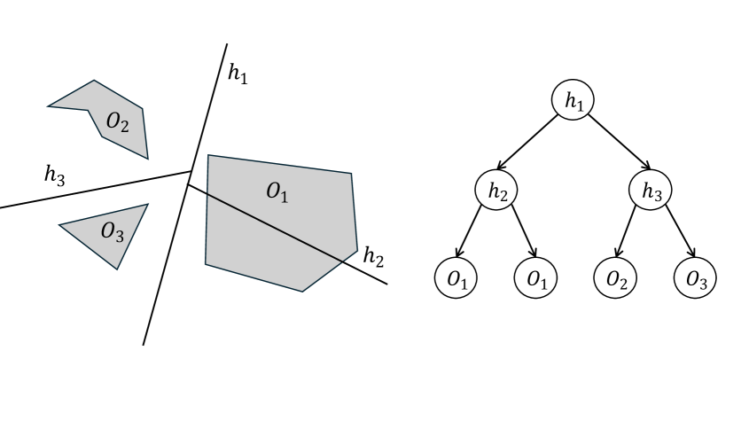
Figure 5. A binary space partition (left) of objects $O_{1}$, $O_{2}$ and $O_{3}$ using hyperplanes $h_{1}$, $h_{2}$, and $h_{3}$, and the corresponding binary space partition tree (right).

Binary space partitioning (BSP) arose from the need in computer graphics to rapidly draw three-dimensional scenes composed of some physical objects. A simple way to draw such scenes is painter’s algorithm: draw polygons in order of distance from the viewer, back to front, painting over the background and previous polygons with each closer object. The objects are then scanned in this so-called depth order, starting with the one farthest from the viewpoint.

However, successfully applying painter’s algorithm depends on the ability to quickly sort objects by depth, which is not always trivial. In some cases, a strict depth ordering may not exist. In such cases, objects must be subdivided into pieces before sorting. To implement the painter’s algorithm in a real-time environment, such as flight simulation, preprocessing the scene is essential to ensure that a valid rendering order can be determined efficiently for any viewpoint.

A BSP tree provides an elegant solution to this problem, which is essentially a decision tree in which each leaf node contains at most one polygon (or it can be empty), with splitting rules defined by hyperplanes. For instance, consider the 2D case; the left panel of figure 5 illustrates the situation where the splitting rules are defined by hyperplanes, and the objects are polygons.

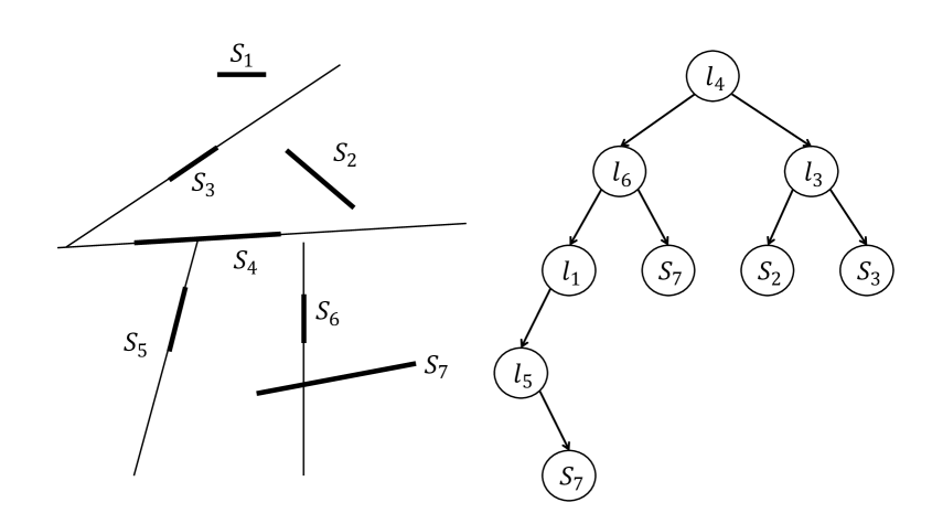
Figure 6. The auto-partition (left) for segments $S_{1}$, $S_{2}$, $S_{3}$, $S_{4}$, $S_{5}$, $S_{6}$, $S_{7}$, and the corresponding binary space partition tree (right). We denote the extending lines for segment $S_{i}$ as $l_{i}$.

To make painter’s algorithm efficient, the resulting BSP tree should be as small as possible in the sense that it has a minimal number of leaf nodes and splitting rules. In theory, the splitting rules used to define the BSP tree can be arbitrary. However, since BSP is primarily applied to problems that require highly efficient solutions—such as dynamically rendering a scene in real time—the splitting rules are typically chosen based on segments (or, in the three-dimensional case, affine flats created by 2D polygons) present in the diagram. A BSP tree that uses only these segments to define splitting rules is called an auto-partition, and we will refer to these rules as auto-rules. For example, as shown in figure 6, when the objects being partitioned are segments, the auto-rules generated by these segments are their extending lines.

The most common algorithm for creating a BSP tree involves randomly choosing permutations of auto-rules and then selecting the best permutation (Motwani and Raghavan, 1996; De Berg, 2000), although the exhaustiveness of permutations has not been properly analyzed in any previous research. While auto-partitions cannot always produce a minimum-size BSP tree, previous probability analyses have shown that the BSP tree created by randomly selecting auto-rules can still produce reasonably small trees, with an expected size of $O\left(N\log N\right)$ for 2D objects and $O\left(N^{2}\right)$ for 3D objects, where $N$ is the number of auto-rules (Motwani and Raghavan, 1996).

For a BSP tree, any splitting rule can become the root, but some segments may split others into two, thereby creating new splitting rules, as seen in figure 6, where segment $S_{7}$ is split into two. Therefore, we need to modify the $\mathit{splits}$ function by defining it as

(21) $$\mathit{splits}_{\text{BSP}}\left(\mathit{rs}\right)=\left[\left(\mathit{sp}_{\text{BSP}}\left(r_{i},\mathit{rs}\right),r_{i},\mathit{sn}_{\text{BSP}}\left(r_{i},\mathit{rs}\right)\right)\mid r_{i}\leftarrow rs\right],$$

where $\mathit{sp}_{\text{BSP}}:\mathcal{R}\to\left[\mathcal{R}\right]\to\left[\mathcal{R}\right]$ and $\mathit{sn}_{\text{BSP}}:\mathcal{R}\to\left[\mathcal{R}\right]\to\left[\mathcal{R}\right]$ are short for “split positive” and “split negative”, respectively. These functions take a splitting rule $r$ and a list of rules $\mathit{rs}$ and return all segments lying on the positive and negative sides of $r$, respectively, including the newly generated rules. At the same time, we need to modify the objective function by simply counting the number of leaf nodes and branch nodes

(22) $$E_{\text{BSP}} :\mathit{DTree}\left(\mathcal{R},\mathcal{D}\right)\to\mathbb{N}$$

$$E_{\text{BSP}} \left(\mathit{DL}\left(\mathit{xs}\right)\right)=1$$

$$E_{\text{BSP}} \left(\mathit{DN}\left(u,r,v\right)\right)=E\left(u\right)+E\left(v\right)+1.$$

The BSP tree produced by the $\mathit{sodt}$ algorithm can, by definition, achieve the minimal size tree with respect to a given set of auto-rules, with a worst-case complexity of $O\left(K!\times N\right)$. By contrast, the classical randomized algorithm always checks all possible permutations in all scenarios to obtain the minimal BSP tree, requiring provably more computations compared to the worst-case scenario of the $\mathit{sodt}$ algorithm. This is because calculating permutations involves additional steps to transform them into trees, and several permutations may correspond to the same tree.

Moreover, the BSP tree is a very general data structure that encompasses several well-known structures, including the $K$-D tree, the max-margin tree ($\mathit{MM}$-tree), and random-projection tree (RP-tree) (Fan et al., 2018, 2019). We will explore how to construct optimal $K$-D tree shortly.

4.2. Optimal decision tree problems with axis-parallel, hyperplane or hypersurface splitting rules

Figure 7. An axis-parallel decision tree model (left), a hyperplanes (oblique) decision tree model (middle), and a hypersurface (defined by degree-$2$ polynomials) decision tree model (right). As the complexity of the splitting functions increase, the tree’s complexity decreases (involving fewer splitting nodes), while achieving higher accuracy.

As discussed in the introduction, due to the intractable combinatorics of the decision tree problem, studies on the ODT problem with even axis-parallel splitting rules are scarce, let alone research on the ODT problem for hyperplanes or more complex hypersurface splitting rules.

However, the more complex the splitting rules, the simpler and more accurate the resulting tree tends to be. To illustrate, Figure 7 three different decision tree models—the axis-parallel, the hyperplane, and the hypersurface decision tree (defined by a degree-two polynomial)—used to classify the same dataset. As the complexity of the splitting rule increases, the resulting decision tree becomes simpler and more accurate. The $\mathit{odt}$ algorithm that we propose will solve all these problems exactly in polynomial time. We now discuss how to approach this problem in more detail.

Unlike the BSP problem, where splitting rules are predefined, for the ODT problem in machine learning, the splitting rules are unknown. The algorithm must learn the best set of rules that will yield the best partition. Therefore, we need a separate process to generate all possible splitting rules in $\mathbb{R}^{D}$. At first glance, the number of possible splitting rules for any given type appears infinite, as the space is continuous. Despite the apparent infinitude of possible splitting rules, the finiteness of the dataset constrains the number of distinct partitions that these rules can generate. This implies the existence of equivalence classes among different rules. It can be proven that the number of equivalence classes for axis-parallel, hyperplane, and hypersurface (defined by degree-$M$ polynomials) decision trees are $O\left(N\times D\right)$, $O\left(N^{D}\right)$ and $O\left(N^{G}\right)$, respectively, where $G=\left(\begin{array}[]{c}D+M\\ D\end{array}\right)-1$ and $N$ is the number of data items. Since the primary focus of this paper is not on combinatorial geometry, we ignore the detailed proof. The intuition behind this combinatorial analysis stems from the fact that axis-parallel, hyperplane, and hypersurface splitting rules can all be defined through combinations of data points.

Assume data points are in general position, meaning no $d+2$ points lies on $d$-dimensional affine flats. The axis-parallel hyperplane has only one degree of freedom, which can be uniquely determined by one data point. Since there are $D$ possible dimensions, there are$N\times D$ possible splitting rules in total. Similarly, a hyperplane in $\mathbb{R}^{D}$ can be uniquely characterized by $D$ data points. Therefore, enumerating all possible hyperplanes in $\mathbb{R}^{D}$ requires $\left(\begin{array}[]{c}N\\ D\end{array}\right)=O\left(N^{D}\right)$ time. Lastly, the hypersurface defined by a degree-$M$ polynomial is isomorphic to a hyperplane in $\mathbb{R}^{G}$. Thus, it can be characterized by using $G$ data points, and all possible hypersurface rules can be enumerated in $O\left(N^{G}\right)$ time.

Therefore, the splitting rule generation process can be done using a combination generator, while the$\mathit{odt}$ and $\mathit{sodt}$ algorithms remain unchanged. This results in a complexity of $O\left(N\times D+K!\times N\times\left(N\times D\right)^{K}\right)=O\left(N^{K}\right)$ for axis-parallel splitting rules, $O\left(N^{D}+K!\times N\times\left(N^{D}\right)^{K}\right)=O\left(N^{DK}\right)$ for hyperplane splitting rules, and $O\left(N^{G}+K!\times N\times\left(N^{G}\right)^{K}\right)=O\left(N^{GK}\right)$ for hypersurface splitting rules.

Even better, with the help of an ingenious combination generator, such as the one developed (He and Little, 2024), we can create the ODT with mixed splitting rules—where axis-parallel, hyperplane, and hypersurface splitting rules are used simultaneously within the same tree. In contrast, classical approaches can only assume one type of splitting rule. To the best of our knowledge, such a decision tree with mixed splitting rules has not been described previously.

4.3. Matrix chain multiplication problem

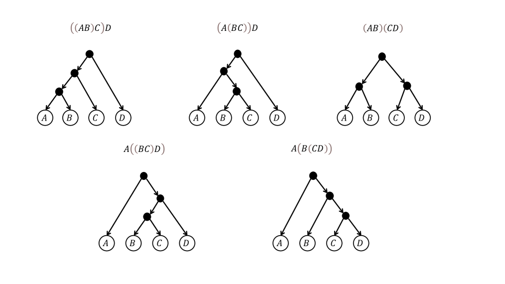
Figure 8. The possible parenthesizations for multiplication of four matrices $A$, $B$, $C$, $D$ correspond to the leaf-labeled trees below, where solid black nodes are the branch nodes that contain no information, and each leaf node stores a matrix.

The special case of our algorithm for the matrix chain multiplication problem (MCMP) was explored previously by Bird and Gibbons (2020). The only modification needed for the MCMP is that the branch nodes become vacuous nodes, containing no information. Alternatively, as Bird and Gibbons (2020) have shown, we can simply delete the branch nodes and define the tree as

$$\mathit{Tree}_{\text{MCMP}}\left(\mathcal{A}\right)=L\left(\mathcal{A}\right)\mid N\left(\mathit{Tree}_{\text{MCMP}}\left(\mathcal{A}\right),\mathit{Tree}_{\text{MCMP}}\left(\mathcal{A}\right)\right).$$

In the case of the MCMP problem, for $N$ matrices stored in a list, we can think of the MCMP as the number of ways to associate parenthesizations of the $N$ matrices. For instance, when $N=4$, as demonstrated in Figure 8, there are five possible parenthesizations:$\left(\left(AB\right)C\right)D$, $\left(A\left(BC\right)\right)D$, $\left(AB\right)\left(CD\right)$, $A\left(\left(BC\right)D\right)$, and $A\left(B\left(CD\right)\right)$.

The only modification we need to make is to the $\mathit{splits}$ function. Similar to the BSP problem, the splits can be arbitrary, but here we do not require any rules to be the root. Therefore, we can define the $\mathit{splits}$ function by simply splitting a sequence of matrices into a pair of non-empty sub-sequences. In other words, if all matrices are stored in a list $\mathit{rs}$ then we want to know all possible partitions $\mathit{ys}$ and $\mathit{zs}$ such that $\mathit{rs}=\mathit{ys}\cup\mathit{zs}$. Hence, the $\mathit{splits}_{\text{MCMP}}$ function, as shown by Bird and Gibbons (2020), can be defined as

$$\mathit{splits}_{\text{MCMP}} \left(\left[\right]\right)=\left[\right]$$

$$\mathit{splits}_{\text{MCMP}} \left(\left[r\right]\right)=\left[\right]$$

$$\mathit{splits}_{\text{MCMP}} \left(r:\mathit{rs}\right)=\left(r,\mathit{rs}\right):\left[\left(x:\mathit{ys},\mathit{zs}\right)\mid\left(\mathit{ys},\mathit{zs}\right)\leftarrow\mathit{splits}_{\text{MCMP}}\left(\mathit{rs}\right)\right].$$

This method of splitting a list of rules is analogous to the calculation of the Catalan number, which implies that any combinatorial objects counted by Catalan numbers can be generated in this way. Stanley and Fomin (1999) described 66 different interpretations of the Catalan numbers. Indeed, Demirović et al. (2022) explicitly employed the $\mathit{splits}_{\text{MCMP}}$ in their recursion and claimed it to be one of their main contributions. However, as we have shown previously, this is an inappropriate splitting function for the decision tree problem in machine learning.

4.4. $K$-D tree

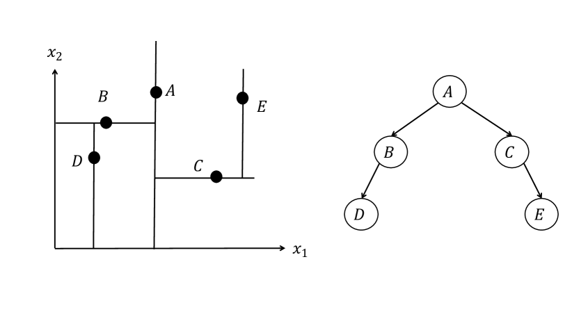
Figure 9. A $K$-D contains seven data points. The split axis for branch nodes at the same level is consistent. Node $A$ splits along the first coordinate,$x_{1}$, while nodes $B$ and $C$ split along the second coordinate, $x_{2}$. Nodes $D$ and $E$ then split along the first coordinate, $x_{1}$, once again.

The $K$-D tree is a fundamental data structure designed for efficiently processing multi-dimensional search queries. Introduced by Bentley (1975) in 1975, it shares similarities with the axis-parallel decision tree model in machine learning. The key distinction lies in the branching rules: while axis-parallel decision trees allow branch nodes to be defined by arbitrary axis-aligned splitting rules, $K$-D trees impose a constraint in which all branch nodes at the same level must follow a predefined splitting rule based on a specific dimension.

For instance, in the $K$-D tree illustrated in Figure 9, the root node applies a splitting rule based on the horizontal axis. Then the splitting axis alternates between the vertical and horizontal axes at each subsequent level.

Similar to an axis-parallel hyperplane decision tree, where possible splitting rules are derived from the data—each dimension having $O\left(N\right)$ choices—resulting in a total of $O\left(N\times D\right)$ possible splits. However, the K-D tree imposes an additional constraint: all splits at the same level must occur along a fixed dimension. This restriction reduces the combinatorial complexity of the problem, as it limits the consideration to $O\left(N\right)$ possible splits, each corresponding to one of the $O\left(N\right)$ data points along a predetermined dimension. Consequently, the tree data type must be redefined to incorporate dimension information at the root of each subtree. This can be achieved by pairing each branch node of the tree with a natural number:

$$\mathit{Tree}_{\text{KD}}\left(\mathcal{A},\mathcal{B}\right)=L\left(\mathcal{B}\right)\mid N\left(\mathit{Tree}_{\text{KD}}\left(\mathcal{A},\mathcal{B}\right),\left(\mathcal{A},\mathbb{N}\right),\mathit{Tree}_{\text{KD}}\left(\mathcal{A},\mathcal{B}\right)\right).$$

Also, the $\mathit{splits}$ function is redefined to incorporate the tree’s depth information, formally expressed as:

$$\mathit{splits}_{\text{KD}} \left(d,\mathit{xs}\right)=\left[\left(\mathit{sp}_{\text{KD}}\left(x,d,\mathit{xs}\right),x,\mathit{sn}_{\text{KD}}\left(x,\mathit{xs}\right)\right)\mid x\leftarrow xs\right],$$

where $\mathit{xs}$ represents a list of data points in $\mathbb{R}^{D}$. The function $\mathit{sp}_{\text{KD}}$ takes a root node $x_{i}$ and outputs all data points in $\mathit{xs}$ whose $d$th coordinate is smaller than that of$x$. Similarly, the function $\mathit{sn}_{\text{KD}}$ selects all data points in $\mathit{xs}$ with greater $d$th coordinates than $x$.

Since $K$-D trees have numerous applications, including nearest neighbor search (finding the closest point(s) to a given query point in a dataset), range search (retrieving all points within a specified range or bounding box), and image processing (feature matching or clustering in multi-dimensional feature spaces), the definition of the objective function depends on the specific application requirements. By combining the $\mathit{splits}_{\text{KD}}$ functions with the$\mathit{odt}$ program, we can construct an optimal $K$-D tree tailored to a given objective function.

5. Discussion and future work

In this paper, we set out four novel axioms that formally define what we refer to as proper decision trees, and then prove that proper decision trees can be characterized as $K$-permutations. This allows us to formally analyze the combinatorial and algorithmic properties of proper decision trees. We then derive a polynomial-time algorithm for the specification by using equational reasoning.

After several rounds of derivation, we obtain a directly executable program for solving the ODT problem that is both elegant and concise. Although the use of formal reasoning to derive programs—particularly in establishing the equivalence of different programs—introduces additional complexity in algorithm design, we argue that such rigor is indispensable for the development of exact algorithms, and we defend this claim with the following two reasons.

Firstly, as we see, defining the complex definition of $\mathit{genDTs}$ directly is difficult and error-prone, whereas, defining $\mathit{genBTs}$ is relatively easy, as it involves only the structure of the tree. Based on the definition of $\mathit{genBTs}$, we can derive the definition of $\mathit{genDTs}$ simply and safely. This highlights a key advantage of the equational reasoning style of derivation: its ability to separate the concerns of efficiency and implementability. Our approach consistently begins with a clear, albeit potentially inefficient, specification, from which we subsequently derive an efficient algorithm.

Secondly, as demonstrated by this problem, numerous studies have reported incorrect results even for the relaxed decision tree problems. There are subtle details that are easy to overlook, and errors resulting from these omissions are difficult to detect without equational reasoning. For instance, previously, we have the following intermediate step for program fusion

(23) $$\mathit{minR}_{E}\bigg{[}\mathit{DN}\bigg{(}\mathit{minR}_{E}\left(\mathit{mapL}{}_{\mathit{\mathit{mapD}}{}_{\cap_{r_{i}^{+}}}}\left(\mathit{genDTs}\left(rs^{+}\right)\right)\right),r_{i},$$

$$\quad\quad\mathit{minR}_{E}\left(\mathit{mapL}{}_{\mathit{\mathit{mapD}}{}_{\cap_{r_{i}^{-}}}}\left(\mathit{genDTs}\left(rs^{-}\right)\right)\right)\bigg{)}\mid\left(\mathit{rs}^{+},r_{i},\mathit{rs}^{-}\right)\leftarrow\mathit{splits}\left(\mathit{rs}\right)\bigg{]},$$

where $\mathit{genDTs}$ is not parameterized with $\mathit{xs}$. If we want to obtain the final recursive program, which, here should be a simple recursive pattern, such as $\mathit{minR}_{E}\left(\mathit{genDTs}\left(rs^{+}\right)\right)$, then, because $\mathit{sodt}\left(\mathit{rs}^{+}\right)=\mathit{minR}_{E}\left(\mathit{genDTs}\left(rs^{+}\right)\right)$, we will have an elegant recursive solution. However, as we can see above, the real-world is not like this. There is a map function $mapL_{\mathit{mapD}{}_{\cap_{r_{i}^{-}}}}$ between $\mathit{minR}_{E}$ and $\mathit{genDTs}$. Changing the definition of $\mathit{genDTs}$ (to make it parameterized by $\mathit{xs}$) is the only way that we can come up with to fuse the $mapL_{\mathit{mapD}{}_{\cap_{r_{i}^{-}}}}$ function inside the definition of $\mathit{genDTs}$. Then we have a recursive definition for $\mathit{sodt}$. However, without presenting all the intermediate fusion steps, such as (23), we will directly fuse the program to obtain

(24) $$\mathit{sodt}\left(\mathit{\mathit{rs}}\right) =\mathit{minR}_{E}\bigg{[}\mathit{DN}\bigg{(}\mathit{mapD}{}_{\cap_{r_{i}^{+}}}\left(\mathit{sodt}\left(\mathit{rs}^{+}\right)\right),r_{i},\mathit{mapD}{}_{\cap_{r_{i}^{+}}}\left(\mathit{sodt}\left(\mathit{rs}^{-}\right)\right)\bigg{)}\mid$$

$$\quad\quad\quad\quad\quad\left(\mathit{rs}^{+},r_{i},\mathit{rs}^{-}\right)\leftarrow\mathit{splits}\left(\mathit{rs}\right)\bigg{]},$$

which updates the information in the leaves after obtaining the optimal subtree $\mathit{sodt}\left(\mathit{rs}^{+}\right)$. Although the above definition resembles the one provided earlier, it is incorrect, as $\mathit{sodt}\left(\mathit{rs}^{-}\right)$ still returns the optimal subtree with respect to the original dataset. This kind of subtle mistake is particularly difficult to detect without deriving the algorithm through equational reasoning.

There are several interesting topics worth exploring in future work. First, the decision tree problem with splitting rules defined as hypersurfaces is an example which satisfies the proper decision tree axioms. Developing the first algorithm for solving this problem would be a significant advancement for the study of interpretable machine learning. Moreover, focusing on a specific problem enables the design of tailored bounding techniques, which are frequently used in the BnB method to further accelerate the algorithm. Such an algorithm would have tremendous impact on interpretable machine learning research especially in high-stakes applications, as numerous studies have shown that tree models still outperform deep neural networks for tabular data, where the data is structured and each feature is meaningful (Grinsztajn et al., 2022; Shwartz-Ziv and Armon, 2022). Also, many studies of optimal decision tree problems (Bertsimas and Dunn, 2017; Rudin, 2019), even though some of them might have errors and therefore be non-optimal, have shown that they still outperform current state-of-art approximate decision tree algorithms, such as CART and C4.5.

Lastly, while memoization is generally impractical for most decision tree problems, it may be feasible to store the root and subtrees in the case of axis-parallel decision trees or a more relaxed variant, such as decision trees for binary feature data. This feasibility arises because there are only $O\left(ND\right)$ possible splitting rules. However, more sophisticated algorithms and data structures are required to manage memoization efficiently.

References

- (1)
- Aghaei et al. (2019) Sina Aghaei, Mohammad Javad Azizi, and Phebe Vayanos. 2019. Learning optimal and fair decision trees for non-discriminative decision-making. In Proceedings of the AAAI Conference on Artificial Intelligence, Vol. 33. 1418–1426.
- Aghaei et al. (2021) Sina Aghaei, Andrés Gómez, and Phebe Vayanos. 2021. Strong optimal classification trees. ArXiv preprint ArXiv:2103.15965 (2021).
- Aglin et al. (2020) Gaël Aglin, Siegfried Nijssen, and Pierre Schaus. 2020. Learning optimal decision trees using caching branch-and-bound search. In Proceedings of the AAAI Conference on Artificial Intelligence, Vol. 34. 3146–3153.
- Aglin et al. (2021) Gaël Aglin, Siegfried Nijssen, and Pierre Schaus. 2021. Pydl8. 5: a library for learning optimal decision trees. In Proceedings of the Twenty-Ninth International Conference on International Joint Conferences on Artificial Intelligence. 5222–5224.
- Avellaneda (2020) Florent Avellaneda. 2020. Efficient inference of optimal decision trees. In Proceedings of the AAAI Conference on Artificial Intelligence, Vol. 34. 3195–3202.
- Barros et al. (2011) Rodrigo C Barros, Ricardo Cerri, Pablo A Jaskowiak, and André CPLF De Carvalho. 2011. A bottom-up oblique decision tree induction algorithm. In 11th International Conference on Intelligent Systems Design and Applications. IEEE, 450–456.
- Bellman (1954) Richard Bellman. 1954. The theory of dynamic programming. Bull. Amer. Math. Soc. 60, 6 (1954), 503–515.
- Bennett (1992) Kristin P Bennett. 1992. Decision tree construction via linear programming. Technical Report. University of Wisconsin-Madison Department of Computer Sciences.
- Bennett and Blue (1996) Kristin P Bennett and Jennifer A Blue. 1996. Optimal decision trees. Rensselaer Polytechnic Institute Math Report 214, 24 (1996), 128.
- Bentley (1975) Jon Louis Bentley. 1975. Multidimensional binary search trees used for associative searching. Commun. ACM 18, 9 (1975), 509–517.
- Bertsimas and Dunn (2017) Dimitris Bertsimas and Jack Dunn. 2017. Optimal classification trees. Machine Learning 106 (2017), 1039–1082.
- Bertsimas and Dunn (2019) Dimitris Bertsimas and Jack Dunn. 2019. Machine learning under a modern optimization lens. Dynamic Ideas LLC Charlestown, MA.
- Bird (2010) Richard Bird. 2010. Pearls of functional algorithm design. Cambridge University Press.
- Bird and De Moor (1996) Richard Bird and Oege De Moor. 1996. The algebra of programming. NATO ASI DPD 152 (1996), 167–203.
- Bird and Gibbons (2020) Richard Bird and Jeremy Gibbons. 2020. Algorithm Design with Haskell. Cambridge University Press.
- Bird (1987) Richard S Bird. 1987. An introduction to the theory of lists. In Logic of Programming and Calculi of Discrete Design: International Summer School directed by FL Bauer, M. Broy, EW Dijkstra, CAR Hoare. Springer, 5–42.
- Breiman (2001a) Leo Breiman. 2001a. Random forests. Machine learning 45 (2001), 5–32.
- Breiman (2001b) Leo Breiman. 2001b. Statistical modeling: the two cultures (with comments and a rejoinder by the author). Statistical science 16, 3 (2001), 199–231.
- Breiman et al. (1984) L. Breiman, J. Friedman, C.J. Stone, and R.A. Olshen. 1984. Classification and Regression Trees. Taylor & Francis. https://books.google.co.uk/books?id=JwQx-WOmSyQC
- Cai et al. (2020) Yuliang Cai, Huaguang Zhang, Qiang He, and Jie Duan. 2020. A novel framework of fuzzy oblique decision tree construction for pattern classification. Applied Intelligence 50 (2020), 2959–2975.
- De Berg (2000) Mark De Berg. 2000. Computational geometry: algorithms and applications. Springer Science & Business Media.
- De Moor (1994) Oege De Moor. 1994. Categories, relations and dynamic programming. Mathematical Structures in Computer Science 4, 1 (1994), 33–69.
- de Moor and Gibbons (1999) Oege de Moor and Jeremy Gibbons. 1999. Bridging the algorithm gap: A linear-time functional program for paragraph formatting. Science of Computer Programming 35, 1 (1999), 3–27. https://doi.org/10.1016/S0167-6423(99)00005-2
- Demirović et al. (2022) Emir Demirović, Anna Lukina, Emmanuel Hebrard, Jeffrey Chan, James Bailey, Christopher Leckie, Kotagiri Ramamohanarao, and Peter J Stuckey. 2022. Murtree: optimal decision trees via dynamic programming and search. Journal of Machine Learning Research 23, 26 (2022), 1–47.
- Fan et al. (2018) Xuhui Fan, Bin Li, and Scott Sisson. 2018. The binary space partitioning-tree process. In International Conference on Artificial Intelligence and Statistics. PMLR, 1859–1867.
- Fan et al. (2019) Xuhui Fan, Bin Li, and Scott Anthony Sisson. 2019. The binary space partitioning-tree process. arXiv preprint arXiv:1903.09343 (2019).
- Galil and Giancarlo (1989) Zvi Galil and Raffaele Giancarlo. 1989. Speeding up dynamic programming with applications to molecular biology. Theoretical Computer Science 64, 1 (1989), 107–118.
- Gibbons (1991) Jeremy Gibbons. 1991. Algebras for tree algorithms. Ph. D. Dissertation. University of Oxford.
- Gibbons (1996) Jeremy Gibbons. 1996. Computing downwards accumulations on trees quickly. Theoretical Computer Science 169, 1 (1996), 67–80.
- Grinsztajn et al. (2022) Léo Grinsztajn, Edouard Oyallon, and Gaël Varoquaux. 2022. Why do tree-based models still outperform deep learning on typical tabular data? Advances in Neural Information Processing Systems 35 (2022), 507–520.
- Günlük et al. (2021) Oktay Günlük, Jayant Kalagnanam, Minhan Li, Matt Menickelly, and Katya Scheinberg. 2021. Optimal decision trees for categorical data via integer programming. Journal of Global Optimization 81 (2021), 233–260.
- He and Little (2023) Xi He and Max A Little. 2023. An efficient, provably exact algorithm for the 0-1 loss linear classification problem. ArXiv preprint ArXiv:2306.12344 (2023).
- He and Little (2024) Xi He and Max A Little. 2024. EKM: an exact, polynomial-time algorithm for the -medoids problem. ArXiv preprint ArXiv:2405.12237 (2024).
- Hu et al. (2020) Hao Hu, Mohamed Siala, Emmanuel Hebrard, and Marie-José Huguet. 2020. Learning optimal decision trees with MaxSAT and its integration in AdaBoost. In 29th International Joint Conference on Artificial Intelligence and the 17th Pacific Rim International Conference on Artificial Intelligence.
- Hu et al. (2019) Xiyang Hu, Cynthia Rudin, and Margo Seltzer. 2019. Optimal sparse decision trees. Advances in Neural Information Processing Systems 32 (2019).
- Ibaraki (1977) Toshihide Ibaraki. 1977. The power of dominance relations in branch-and-bound algorithms. J. ACM 24, 2 (1977), 264–279.
- Jia et al. (2019) Su Jia, Fatemeh Navidi, R Ravi, et al. 2019. Optimal decision tree with noisy outcomes. Advances in Neural Information Processing Systems 32 (2019).
- Karp and Held (1967) Richard M Karp and Michael Held. 1967. Finite-state processes and dynamic programming. SIAM J. Appl. Math. 15, 3 (1967), 693–718.
- Laurent and Rivest (1976) Hyafil Laurent and Ronald L Rivest. 1976. Constructing optimal binary decision trees is NP-complete. Inform. Process. Lett. 5, 1 (1976), 15–17.
- Lin et al. (2020) Jimmy Lin, Chudi Zhong, Diane Hu, Cynthia Rudin, and Margo Seltzer. 2020. Generalized and scalable optimal sparse decision trees. International Conference on Machine Learning, 6150–6160.
- Little et al. (2021) Max A Little, Xi He, and Ugur Kayas. 2021. Dynamic programming by polymorphic semiring algebraic shortcut fusion. ArXiv preprint ArXiv:2107.01752 (2021).
- Mazumder et al. (2022) Rahul Mazumder, Xiang Meng, and Haoyue Wang. 2022. Quant-BnB: A scalable branch-and-bound method for optimal decision trees with continuous features. In International Conference on Machine Learning. PMLR, 15255–15277.
- Motwani and Raghavan (1996) Rajeev Motwani and Prabhakar Raghavan. 1996. Randomized algorithms. ACM Computing Surveys (CSUR) 28, 1 (1996), 33–37.
- Murthy et al. (1994) Sreerama K Murthy, Simon Kasif, and Steven Salzberg. 1994. A system for induction of oblique decision trees. Journal of Artificial Intelligence Research 2 (1994), 1–32.
- Narodytska et al. (2018) Nina Narodytska, Alexey Ignatiev, Filipe Pereira, and Joao Marques-Silva. 2018. Learning optimal decision trees with SAT. In 27th International Joint Conference on Artificial Intelligence. International Joint Conferences on Artificial Intelligence Organization, 1362–1368. https://doi.org/10.24963/ijcai.2018/189
- Nijssen and Fromont (2007) Siegfried Nijssen and Elisa Fromont. 2007. Mining optimal decision trees from itemset lattices. In Proceedings of the 13th ACM SIGKDD international conference on Knowledge discovery and data mining. 530–539.
- Nijssen and Fromont (2010) Siegfried Nijssen and Elisa Fromont. 2010. Optimal constraint-based decision tree induction from itemset lattices. Data Mining and Knowledge Discovery 21 (2010), 9–51.
- Quinlan (2014) J Ross Quinlan. 2014. C4. 5: programs for machine learning. Elsevier.
- Rudin (2019) Cynthia Rudin. 2019. Stop explaining black box machine learning models for high stakes decisions and use interpretable models instead. Nature Machine Intelligence 1, 5 (2019), 206–215.
- Ruskey (2003) Frank Ruskey. 2003. Combinatorial generation. Preliminary working draft. University of Victoria, Victoria, BC, Canada 11 (2003), 20.
- Schmidt and Ströhlein (2012) Gunther Schmidt and Thomas Ströhlein. 2012. Relations and graphs: discrete mathematics for computer scientists. Springer Science & Business Media.
- Sedgewick (1977) Robert Sedgewick. 1977. Permutation generation methods. ACM Computing Surveys (CSUR) 9, 2 (1977), 137–164.
- Shwartz-Ziv and Armon (2022) Ravid Shwartz-Ziv and Amitai Armon. 2022. Tabular data: Deep learning is not all you need. Information Fusion 81 (2022), 84–90.
- Stanley and Fomin (1999) Richard P. Stanley and Sergey Fomin. 1999. Enumerative combinatorics volume 2. Cambridge University Press.
- Tóth (2005) Csaba D Tóth. 2005. Binary space partitions: recent developments. Combinatorial and Computational Geometry 52 (2005), 525–552.
- Verwer and Zhang (2019) Sicco Verwer and Yingqian Zhang. 2019. Learning optimal classification trees using a binary linear program formulation. In Proceedings of the AAAI Conference on Artificial Intelligence, Vol. 33. 1625–1632.
- Wickramarachchi et al. (2016) Darshana Chitraka Wickramarachchi, Blair Lennon Robertson, Marco Reale, Christopher John Price, and Jennifer Brown. 2016. HHCART: an oblique decision tree. Computational Statistics & Data Analysis 96 (2016), 12–23.
- Zhang et al. (2023) Rui Zhang, Rui Xin, Margo Seltzer, and Cynthia Rudin. 2023. Optimal sparse regression trees. In Proceedings of the AAAI Conference on Artificial Intelligence, Vol. 37. 11270–11279.