Leap into the future: shortcut to dynamics for quantum mixtures

Abstract

The study of the long-time dynamics of quantum systems can be a real challenge, especially in systems like ultracold gases, where the required timescales may be longer than the lifetime of the system itself. In this work, we show that it is possible to access the long-time dynamics of a strongly repulsive atomic gas mixture in shorter times. The shortcut-to-dynamics protocol that we propose does not modify the fate of the observables, but effectively jumps ahead in time without changing the system’s inherent evolution. Just like the next-chapter button in a movie player that allows to quickly reach the part of the movie one wants to watch, it is a leap into the future.

Observing and studying quantum phenomena that occur over long timescales can be a daunting task. For example, it can be extremely difficult to distinguish between a very slow thermalization dynamics and a situation where thermalization does not occur Luitz et al. (2015); Alet and Laflorencie (2018), since this requires observing dynamics over a very long time, time in which the quantum system could be deeply perturbed by the coupling with the external environment. Another phenomenon that is interesting to study over a long time, and which can suffer from the decoherence induced by the interaction with the environment, is the coherence spreading. This observable may give access, for instance, to new forms of quantum information transfer Qiao et al. (2020).

When experimental timescales become a limiting factor, the question arises if it is possible to devise a shortcut protocol that fast forwards the dynamics for a given time, thereby reducing the time needed to observe a physical phenomenon of interest. The concept of driving the dynamics has been previously introduced (see for instance Masuda and Nakamura (2008, 2009); Torrontegui et al. (2012, 2013); Martínez-Garaot et al. (2016); Patra and Jarzynski (2017); Guéry-Odelin et al. (2019); Bernardo (2020) and references therein), but as a strategy to speed up an adiabatic evolution to attain a target state or realize a given protocol in a shorter time Chen et al. (2010); Schaff et al. (2010, 2011); del Campo (2011a); del Campo and Boshier (2012); del Campo (2013); Deng et al. (2018); Diao et al. (2018). Here the idea is different: fast-forwarding the dynamics to access the system’s dynamics starting from a time $\tau_{\smalltriangleright\scalebox{0.5}{|}}$ after a time $t_{\smalltriangleright\scalebox{0.5}{|}}\ll\tau_{\smalltriangleright\scalebox{0.5}{|}}$. The goal is not to target a specific quantum state, neither to speed up a specific protocol but rather to jump ahead to the time when we want to start observing the dynamics, just as when we use the next-chapter button to watch the part of the movie that interests us, without needing to know anything of the movie in advance (see Fig. 1).

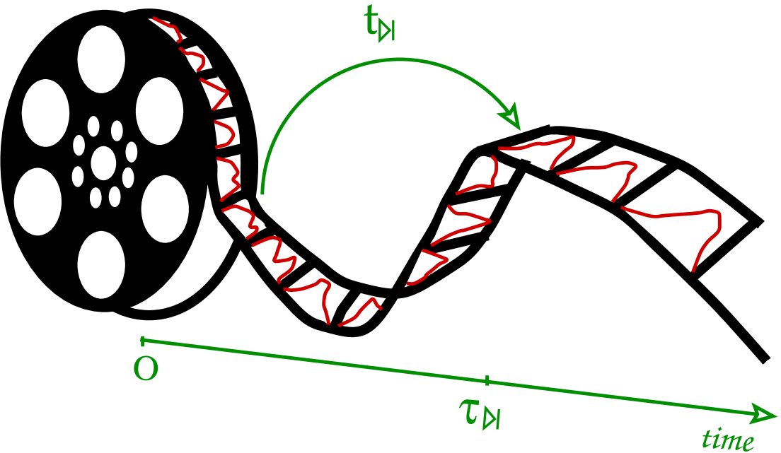
Figure 1: Schematic representation of the shortcut-to-dynamics protocol proposed in this work: a time leap $\tau_{\smalltriangleright\scalebox{0.5}{|}}$ realized in a time $t_{\smalltriangleright\scalebox{0.5}{|}}$, with $t_{\smalltriangleright\scalebox{0.5}{|}}\ll\tau_{\smalltriangleright\scalebox{0.5}{|}}$.

Our protocol applies to one-dimensional (1D) strongly repulsive quantum mixtures Zürn et al. (2012). Such systems can be mapped onto Heisenberg spin chains Deuretzbacher et al. (2014); Volosniev et al. (2016); Aupetit-Diallo et al. (2022) and admit an exact solution in the limit of infinite interactions Volosniev et al. (2014), so that they are a paradigm for the study of the long-time dynamics in the vicinity of integrability Pecci et al. (2022); Musolino et al. (2024). They could also be a good candidate for the study of the interplay between interactions and disorder Capuzzi et al. (2024). In strongly repulsive 1D mixtures, the charge and the spin degrees of freedom separate Arute et al. (2020). More precisely, the dynamics of the different spin components is governed, in addition to the strength of the interaction and the statistics, by the total density, whose evolution, however, does not depend on the inter-component dynamics Deuretzbacher et al. (2008); Volosniev et al. (2014); Deuretzbacher et al. (2014); Pecci et al. (2022); Capuzzi et al. (2024); Musolino et al. (2024).

In this letter, we show that this separation allows to fast-forward the spin-components dynamics up to a time $\tau_{\smalltriangleright\scalebox{0.5}{|}}$ by first compressing and then decompressing the total density during a much shorter time $t_{\smalltriangleright\scalebox{0.5}{|}}$, $\tau_{\smalltriangleright\scalebox{0.5}{|}}$ being a function of $t_{\smalltriangleright\scalebox{0.5}{|}}$, $\tau_{\smalltriangleright\scalebox{0.5}{|}}=\tau(t_{\smalltriangleright\scalebox{0.5}{|}})$. If the compression-decompression cycle is suitably performed such that the total density recovers its initial size at $t_{\smalltriangleright\scalebox{0.5}{|}}$ without further exciting the system, then for $t=t_{\smalltriangleright\scalebox{0.5}{|}}+t^{\prime}$ the system continues the time evolution such as it was at time $\tau_{\smalltriangleright\scalebox{0.5}{|}}+t^{\prime}$: we get a shortcut to dynamics for the spin components.

Model - We consider a fermionic or bosonic spin mixture with $\kappa$ components, trapped in an 1D time-dependent harmonic trap of frequency $\omega(t)$. The mixture obeys the Hamiltonian

$$\begin{split}\hat{H}&=\sum^{\kappa}_{\sigma=1}\sum_{i=1}^{N_{\sigma}}\left[-\frac{\hbar^{2}}{2m}\frac{\partial^{2}}{\partial x_{i,\sigma}^{2}}+\dfrac{1}{2}m\omega(t)^{2}x_{i,\sigma}^{2}\right]+\sum^{\kappa}_{\sigma=1}g_{\sigma\sigma}\\ &\sum_{i=1}^{N_{\sigma}}\sum_{j>i}^{N_{\sigma}}\delta(x_{i,\sigma}-x_{j,\sigma})+\frac{1}{2}\sum^{\kappa}_{\sigma\neq\sigma^{\prime}=1}g_{\sigma\sigma^{\prime}}\sum_{i=1}^{N_{\sigma}}\sum_{j=1}^{N_{\sigma^{\prime}}}\delta(x_{i,\sigma}-x_{j,\sigma^{\prime}}),\\ \end{split}$$ (1)

where $\kappa$ is the number of spin species, $N_{\sigma}$ the number of particles with spin $\sigma$, $g_{\sigma\sigma^{\prime}}$ and $g_{\sigma\sigma}$ are the inter- and intra-species interaction strengths. The latter concerns only identical bosons, since for identical fermions s-wave contact interactions are forbidden. The regime we are interested in is the strongly repulsive one, where $g_{\sigma\sigma}m/(\hbar^{2}n(x=0)\gg 1$ and $g_{\sigma\sigma^{\prime}}m/(\hbar^{2}n(x=0)\gg 1$, for any $\sigma,\sigma^{\prime}$, where $n(x=0)$ is the density at the trap center.

The proposed protocol applies to any mixture that obeys the Hamiltonian (1) in such a regime, one of the key points being the spin-density separation that occurs for strongly repulsive interactions. Nevertheless, in the following, we will focus on the case of a SU(2) balanced fermionic mixture ($\kappa=2$, $g_{\uparrow\uparrow}=g_{\downarrow\downarrow}$, $g_{\uparrow\downarrow}=g$ and $N_{\uparrow}=N_{\downarrow}=N/2$). The system evolution we want to measure at long times is that of the two spin-components in a static harmonic confinement Pecci et al. (2022). The shortcut to dynamics idea is to drive the proper time of the spin components by modifying the harmonic trapping during a short time. For that matter, we will construct the many-body wavefunction for such time-dependent Hamiltonian starting from the many-body wavefunction of the time-independent one. This will allow us to engineer our shortcut-to-dynamics protocol.

The evolution for a time-independent Hamiltonian - As a first step, we consider the evolution of the system under time-independent harmonic trapping, $\omega(t)=\omega_{0}$, $\forall t$, in the absence of charge excitations. In the strongly repulsive regime, the many-body wavefunction, $\Psi(\vec{X},\vec{\sigma},t)$ with $\vec{X}=\{x_{1},x_{2},\dots,x_{N}\}$ and $\vec{\sigma}=\{\sigma_{1},\sigma_{2},\dots,\sigma_{N}\}$, vanishes whenever $x_{i}=x_{j}$. It can be written as follows Deuretzbacher et al. (2008); Volosniev et al. (2014)

$$\Psi(\vec{X},\vec{\sigma},t)=\sum_{P\in S_{N}}\alpha_{P}(t)\theta_{P}(\vec{X})\Xi_{A}(\vec{X}),$$ (2)

where the $\vec{\sigma}$-dependence is hidden in the spin coefficients $\alpha_{P}(t)$, with $P$ permutation of $N$ elements in $S_{N}$. $\theta_{P}(\vec{X})$ is the generalized Heaviside function, which is equal to 1 in the coordinate sector $x_{P(1)}<\dots<x_{P(N)}$ and 0 elsewhere, and $\Xi_{A}=(1/\sqrt{N!})\det[\chi_{j}(x_{k})]$ is the Slater determinant built from the orbitals $\chi_{j}(x)$ of the single-particle Hamiltonian for the harmonic potential, $H_{0}\chi_{j}(x)=\varepsilon_{j}\chi_{j}(x)$, with

$$H_{0}=-\frac{\hbar^{2}}{2m}\frac{\partial^{2}}{\partial x^{2}}+\dfrac{1}{2}m\omega_{0}^{2}x^{2}.$$ (3)

Since there are no charge excitations, $\Xi_{A}$ is time independent, and the many-body evolution is dictated by $\alpha_{P}$.

The time evolution of the $\alpha_{P}(t)$’s coefficients is determined by the effective spin-chain Hamiltonian  Deuretzbacher et al. (2014)

$$H_{S}^{0}=\sum_{j=1}^{N-1}\left(-J_{j}^{0}\hat{1}+J_{j}^{0}\hat{P}_{j,j+1}\right)$$ (4)

where $\hat{P}_{j,j^{\prime}}$ is the permutation operator. The hopping amplitudes $J_{i}^{0}$ in Eq. (4) can be written as

$$J_{i}^{0}=\frac{N!}{g}\int_{-\infty}^{\infty}dX~\delta(x_{i}-x_{i+1})\theta_{\text{id}}(\vec{X})\Bigl{\lvert}\frac{\partial\Xi_{A}}{\partial x_{i}}\Big{\lvert}^{2},$$ (5)

where $\Theta_{\text{id}}(\vec{X})$ is the generalized Heaviside function for the identity permutation. Let $\varepsilon_{S,j}$ and $\alpha_{P}^{j}$ be the eigenvalues and the corresponding eigenvectors of $H_{s}^{0}$. If we write $\alpha_{P}(t=0)=\beta_{j}\alpha_{P}^{j}$, then the evolution of $\alpha_{P}$ is given by

$$\alpha_{P}(t)=\sum_{j}\beta_{j}\alpha_{P}^{j}e^{-i\varepsilon_{S,j}t/\hbar}.$$ (6)

Such a system has a time-independent total density

$$n_{0}(x)=\int dx_{2}\,dx_{3}\dots dx_{N}|\Xi_{A}(x,x_{2},\dots x_{N})|^{2}$$ (7)

and spin-component densities

$$n_{\sigma,0}(x,t)=\sum_{i=1}^{N}\left(\sum_{P}|\alpha_{p}(t)|^{2}\delta_{\sigma,\sigma_{i}}\rho_{0}^{(i)}(x)\right)$$ (8)

where the density of the $i-$th fermion reads

$$\rho_{0}^{(i)}(x)=N!\int_{\mathcal{I}_{i}}\prod_{j\neq i}|\Xi_{A}(x_{1},\dots x_{i-1},c,x_{i+1},\dots,x_{N})|^{2},$$ (9)

$\mathcal{I}_{i}$ being the integration interval constrained by $x_{1}<x_{2}<\dots<x_{i-1}<x<x_{i+1}<\dots<x_{N}$.

If the initial spin state is not an eigenstate of the $H_{S}^{0}$, even if the total density is constant in time, there is a relative motion between the spin components Wei et al. (2022); Pecci et al. (2022); Musolino et al. (2024), so that the density magnetization $m_{0}(x,t)=n_{\uparrow,0}(x,t)-n_{\downarrow,0}(x,t)$ is not constant in time. Following the time-evolution of its center of mass

$$d_{0}(t)=\frac{1}{N}\int dx\,x\,m_{0}(x,t).$$ (10)

one can have access to interesting physical phenomena related to the motion of the spin components such as superdiffusion at short time Wei et al. (2022); Pecci et al. (2022), universal oscillations at intermediate time Pecci et al. (2022), and eventually thermalization at long times Pecci et al. (2022); Capuzzi et al. (2024). In the strongly interacting regime, the timescale for the spin’s motion is $\hbar/J_{i}^{0}$, namely, it scales with the particle’s interaction strength so that it can be very large with respect to the harmonic oscillator period. The observation of the spin dynamics at long times can therefore become difficult to access due to the finite lifetime of the trapped system. Our goal will be to have access to the spin dynamics for $t>\tau_{\smalltriangleright\scalebox{0.5}{|}}$ after a time with $t_{\smalltriangleright\scalebox{0.5}{|}}\ll\tau_{\smalltriangleright\scalebox{0.5}{|}}$. In particular, we shall focus our analysis on the evolution of the spin-component densities $n_{\sigma,0}(x,t)$ and the magnetization center of mass $d_{0}(t)$.

The evolution for the time-dependent Hamiltonian - When the trap frequency depends on time, the evolution of the many-body wavefunction admits a scaling solution that keeps the same form as the one for the time-independent problem

$$\Psi(\vec{X},\vec{\sigma},t)=\sum_{P\in S_{N}}a_{P}(t)\theta_{P}(\vec{X})\Psi_{A}(\vec{X},t),$$ (11)

Here

$$\Psi_{A}(\vec{X},t)=\dfrac{1}{b^{N/2}}\Xi_{A}(\vec{Y})\,e^{\displaystyle-\frac{i}{\hbar}\int_{0}^{t}dt^{\prime}/b^{2}\sum_{j=0}^{N-1}\varepsilon_{j}}\times e^{\displaystyle i\frac{m}{\hbar}\frac{\dot{b}}{2b}\sum_{k=1}^{N}x_{k}^{2}}$$ (12)

is the Slater determinant of the space-and-time rescaled time-dependent one-particle orbitals Minguzzi and Gangardt (2005); Gritsev et al. (2010); Chen et al. (2010); del Campo (2011b); Schaff et al. (2011); Guéry-Odelin et al. (2019)

$$\phi_{j}(x_{k},t)=\dfrac{1}{\sqrt{b}}\chi_{j}(y_{k})e^{\displaystyle-\frac{i}{\hbar}\varepsilon_{j}\int_{0}^{t}dt^{\prime}/b^{2}}\,e^{\displaystyle i\frac{m}{\hbar}\frac{\dot{b}}{2b}x_{k}^{2}}$$ (13)

where $y_{k}=x_{k}/b$ and the scaling function $b(t)$ verifies the Ermakov equation

$$\ddot{b}+\omega^{2}(t)b=\dfrac{\omega_{0}^{2}}{b^{3}}.$$ (14)

The Slater determinant scaling allows us to obtain the scaling properties of the hopping amplitudes $J_{i}(t)$ governing the spin dynamics:

$$\begin{split}J_{i}(t)&=\frac{N!}{g}\int_{-\infty}^{\infty}dX~\delta(x_{i}-x_{i+1})\theta_{\text{id}}(X)\Bigl{\lvert}\frac{\partial\Psi_{A}}{\partial x_{i}}\Big{\lvert}^{2}\\ &=\frac{N!}{g}\int_{-\infty}^{\infty}dX~\delta(x_{i}-x_{i+1})\theta_{\text{id}}(X)\frac{1}{b^{N+2}}\Bigl{\lvert}\frac{\partial\Xi_{A}}{\partial y_{i}}\Big{\lvert}^{2}\\ &\frac{N!}{gb^{3}}\int_{-\infty}^{\infty}dY~\delta(y_{i}-y_{i+1})\theta_{\text{id}}(Y)\Bigl{\lvert}\frac{\partial\Xi_{A}}{\partial y_{i}}\Big{\lvert}^{2}\\ &=\dfrac{J_{i}^{0}}{b^{3}}.\end{split}$$ (15)

This implies that the sector amplitudes $a_{P}$ can be expressed as a function of the ones for the time-independent Hamiltonian $\alpha_{P}$ by rescaling the time. Namely, $a_{P}(t)=\alpha_{P}(\tau)$, with $\tau=\int_{0}^{t}dt^{\prime}/b(t^{\prime})^{3}$. This means that by manipulating the scaling function $b(t)$ through a suitable protocol for $\omega(t)$, one can observe the spin dynamics of the time-independent Hamiltonian at different times $\tau$.

For the time-dependent problem, the total density reads

$$\begin{split}n_{0}(x,t)&=\int dx_{2}\,dx_{3}\dots dx_{N}|\Psi_{A}(x,x_{2},\dots x_{N})|^{2}\\ &=\dfrac{1}{b}n_{0}(x/b)\end{split}$$ (16)

and the density of the $i-$th fermion scales as $\rho^{(i)}(x,t)=1/b\,\rho_{0}^{(i)}(x/b)$. Thus, the spin component densities can be written as

$$\begin{split}n_{\sigma}(x,t)&=\sum_{i=1}^{N}\left(\sum_{P}|a_{p}(t)|^{2}\delta_{\sigma,\sigma_{i}}\rho^{(i)}(x,t)\right)\\ &=\frac{1}{b}\sum_{i=1}^{N}\left(\sum_{P}|\alpha_{p}(\tau(t))|^{2}\delta_{\sigma,\sigma_{i}}\rho_{0}^{(i)}(x/b)\right)\\ &=\dfrac{1}{b}n_{\sigma,0}(x/b,\tau(t)).\end{split}$$ (17)

Analogously, the magnetization can be written as

$$m(x,t)=\frac{1}{b}m_{0}(x/b,\tau(t))$$ (18)

and its center of mass

$$\begin{split}d(t)&=\frac{1}{N}\int dx\,x\,m(x,t)\\ &=b(t)d_{0}(\tau(t)).\end{split}$$ (19)

Remark that if the initial state is an eigenstate of $H_{S}^{0}$, it will be an eigenstate of $H_{S}^{0}/b^{3}$ too. In such a case $\alpha_{p}(\tau(t))=\alpha_{p}^{j}$, so that the magnetization density follows the same scaling law as the total density, namely $m(x,t)=m_{0}(x/b)/b$.

Shortcut-to-dynamics protocol for the spin dynamics - We seek a scaling transformation $b(t)$, and thus a time-dependent trap frequency $\omega(t)$ that can be experimentally realized and that allows to reach our shortcut-to-dynamics goal. We choose the strategy to fast compress and decompress the total density using a shortcut protocol Chen et al. (2010); Schaff et al. (2010, 2011), so that the initial density and the final density for $t\geq t_{\smalltriangleright\scalebox{0.5}{|}}$ are identical, ie, $b(0)=1$ and $b(t\geq t_{\smalltriangleright\scalebox{0.5}{|}})=1$, but the elapsed time for the spin dynamics is significantly longer than the time duration of the compression-decompression cycle. The shortcut protocol implies that $\dot{b}(0)=0$, $\dot{b}(t_{\smalltriangleright\scalebox{0.5}{|}})=0$, $\ddot{b}(0)=0$, $\ddot{b}(t_{\smalltriangleright\scalebox{0.5}{|}})=0$, while the fast-forward condition is fulfilled if $b(0<t<t_{\smalltriangleright\scalebox{0.5}{|}})<1$.

As a specific example, we choose the compression and the decompression times to be equal, by imposing $\dot{b}(t_{\smalltriangleright\scalebox{0.5}{|}}/2)=0$. Proposing a lower order polynomial solution to the Ermakov equation, we can write a solution for the scaling parameter $b$ as

$$b(t)=1-|A|\left(-({t}/{t_{\smalltriangleright\scalebox{0.5}{|}}})^{6}+3(t/t_{\smalltriangleright\scalebox{0.5}{|}})^{5}-3(t/t_{\smalltriangleright\scalebox{0.5}{|}})^{4}+(t/t_{\smalltriangleright\scalebox{0.5}{|}})^{3}\right),$$ (20)

which, in turn, determines the trapping strength through Eq. (14). The amplitude $|A|$ has to be chosen so that $\omega^{2}(t)>0$ to ensure the system remains confined during the shortcut protocol.

In Fig. 2, we show the behaviour of $\omega^{2}(t)/\omega_{0}^{2}$ as a function of $t/t_{\smalltriangleright\scalebox{0.5}{|}}$ for different values of $\tau_{\smalltriangleright\scalebox{0.5}{|}}/t_{\smalltriangleright\scalebox{0.5}{|}}$ that are determined by the value of $|A|$. We observe that longer time leaps require larger variations in trapping strength, and consequently, in density. This must be considered in experimental realizations to avoid the gas leaving the strongly interacting regime that is assured for $gm/(\hbar^{2}n(x=0,t))\gg 1$ for all time.

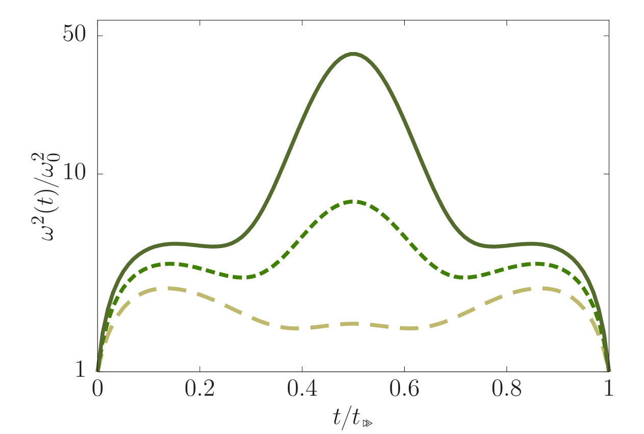
Figure 2: Trapping strength $\omega^{2}(t)/\omega_{0}^{2}$ as a function of $t/t_{\smalltriangleright\scalebox{0.5}{|}}$ for $\tau(t_{\smalltriangleright\scalebox{0.5}{|}})/t_{\smalltriangleright\scalebox{0.5}{|}}$=1.77 ($|A|=20$, long-dashed line), 2.80 ($|A|=30$, short-dashed line), 5.56 ($|A|=40$, solid line).

We have implemented the shortcut-to-dynamics protocol outlined above for the case $|A|=30$, which corresponds to a maximum change of the trapping potential of a factor $\sim 3$ and to a maximum variation of the density at the center of the trap of the $\sim 30\%$ at $t\simeq t_{\smalltriangleright\scalebox{0.5}{|}}/2$. This choice fixes $\tau_{\smalltriangleright\scalebox{0.5}{|}}=2.80t_{\smalltriangleright\scalebox{0.5}{|}}$. We have studied the time evolution of the spin densities (see Fig. 3 for $n_{\uparrow}(t)$) and of the center of mass of the magnetization $d(t)$ (see Fig. 4) for the case of 4+4 SU(2) fermions initially prepared in a domain wall configuration at $x=0$, where the spins up and down are located in the two opposite sides of the trap. In both Figs. 3 and 4, we compare the dynamics with and without using our shortcut-to-dynamics protocol, and we show that the dynamics at a time $t_{\smalltriangleright\scalebox{0.5}{|}}+t^{\prime}$ in the first case coincides with that at a time $\tau_{\smalltriangleright\scalebox{0.5}{|}}+t^{\prime}$ in the second case, as expected.

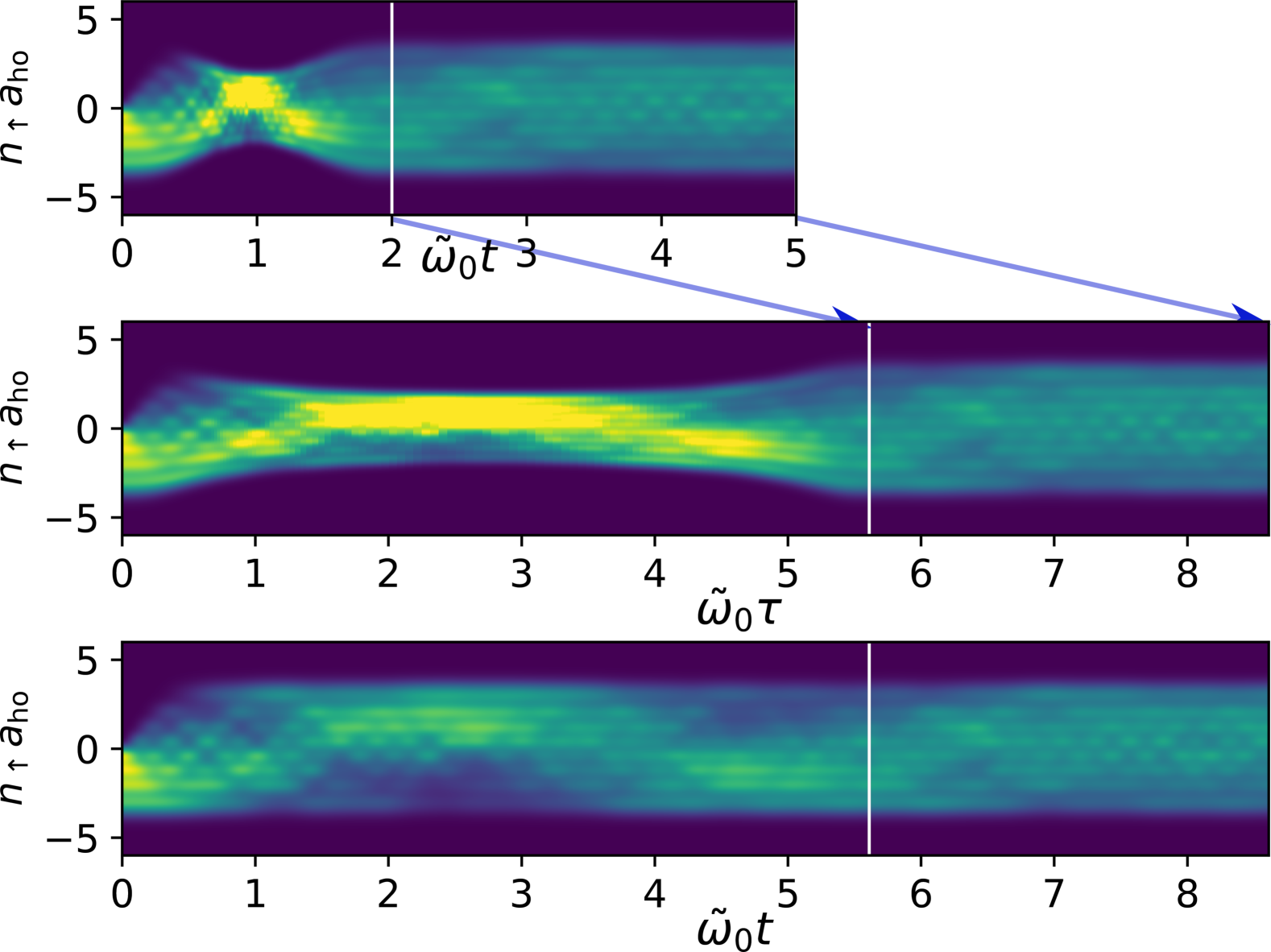
Figure 3: Time evolution of the spin density $n_{\uparrow}(t)$ for a SU(2) fermionic balanced mixture ($N=8$), the initial state being a domain wall. Top panel: Time evolution by applying the shortcut-to-dynamics protocol, as a function of $\tilde{\omega}_{0}t$, with $\tilde{\omega}_{0}=\hbar\omega_{0}^{2}a_{ho}/g$. Middle panel: the same as the top panel but a function of $\tilde{\omega}_{0}\tau(t)$. Bottom panel: Time evolution without applying the shortcut-to-dynamics protocol, as a function of $\tilde{\omega}_{0}t$. The white vertical lines indicate $t_{\smalltriangleright\scalebox{0.5}{|}}$ in the top panel and $\tau(t_{\smalltriangleright\scalebox{0.5}{|}})$ in the middle and bottom panels. The first blue arrow shows the correspondence between $t_{\smalltriangleright\scalebox{0.5}{|}}$ and $\tau_{\smalltriangleright\scalebox{0.5}{|}}$, while the second one shows the correspondence between the final times $t_{F}$ and $\tau(t_{F})$. The spin-down density $n_{\downarrow}(t)$ (not shown in the figure) is the mirror reflection of $n_{\uparrow}(t)$ with respect to the trap center for the particular spin excitation considered in this example.

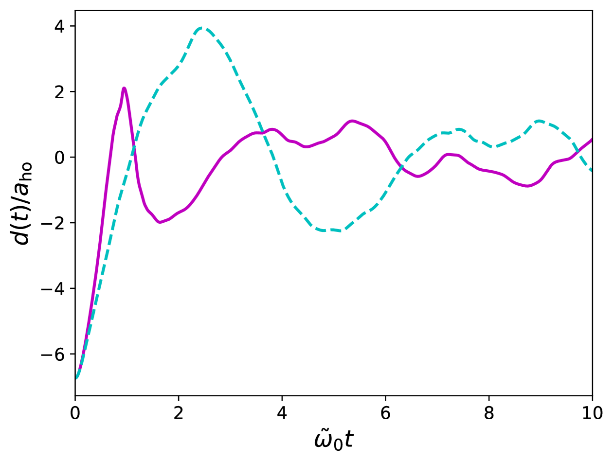
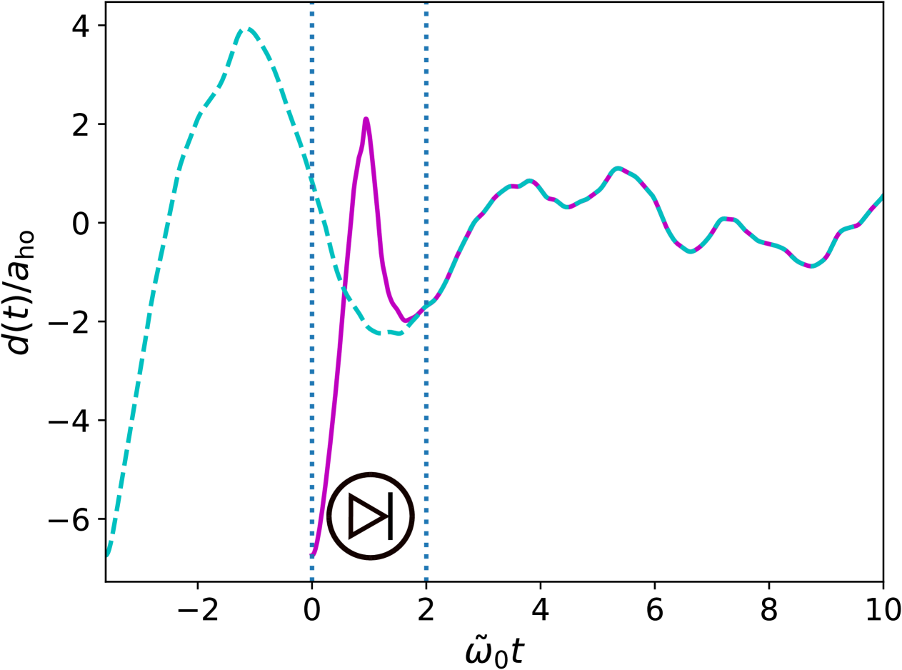
Figure 4: Top panel: The magnetization center of mass $d(t)$ as a function of $\tilde{\omega}_{0}t$, with $\tilde{\omega}_{0}=\hbar\omega_{0}^{2}a_{ho}/g$ for a SU(2) fermionic balanced mixture ($N=8$), the initial state being a domain wall. We study its time-evolution without exciting the total density (cyan dashed curve) and under the action of the shortcut-to-dynamics protocol (magenta solid curve). Bottom panel: same as the top panel, but with the cyan curve plotted as a function of $t-(\tau_{\smalltriangleright\scalebox{0.5}{|}}-t_{\smalltriangleright\scalebox{0.5}{|}})$ with $\tau_{\smalltriangleright\scalebox{0.5}{|}}-t_{\smalltriangleright\scalebox{0.5}{|}}$ being the gained time with the shortcut-to-dynamics protocol. The fast-forward time region has been delimited by the two vertical dashed lines.

We note that the same shortcut-to-dynamics protocol can be repeated several times in the same experiment, so that one can have access to the spin long-time dynamics with a sequence of time leaps. Let us underline once more that the same protocol can be applied to any possible spin excitation in any mixture described by the Hamiltonian (1) in the limit of strong repulsive interactions, namely in situations where the total density behaves as that of a system of non-interacting fermions, and the spin-dynamics is driven by the total density.

Conclusions - We have shown that it is possible to jump forward in the spin dynamics in a strongly repulsive quantum mixture by rapidly compressing and then decompressing the total density. The time $t_{\smalltriangleright\scalebox{0.5}{|}}$ of the compression-decompression cycle is the time needed for the fast-forward process to advance the spin system to a later time $\tau_{\smalltriangleright\scalebox{0.5}{|}}$ of its natural evolution, with $\tau_{\smalltriangleright\scalebox{0.5}{|}}\gg t_{\smalltriangleright\scalebox{0.5}{|}}$. The many-body wavefunction is identical to the one at time $\tau_{\smalltriangleright\scalebox{0.5}{|}}$ except for a global phase factor that does not affect any physical observable, while the spatial component follows a simple scaling equation. Our protocol is analytical for the case of a system that is trapped in a harmonic confinement, but one could look for some numerical protocols for the case of a strongly interacting mixture in the presence of disorder. This would pave the way to an easier access, both numerically and experimentally, to the long-time many-body dynamics of these quantum systems.

As a final remark, one could wonder if a similar fast-backward (previous chapter) protocol would be possible. This would imply a time $\tau_{\smalltriangleright\scalebox{0.5}{|}}$ that is negative, but it wouldn’t be possible by keeping the interaction strength constant. Indeed, even if $b(t)$ were negative, the positivity of the density dictates that $d\tau=dt/|b|^{3}$. $d\tau$ being always positive, it is not possible to bring the spin system to its past. However, a possible strategy could involve sweeping from strongly repulsive to strongly attractive interaction using a confinement induced resonance Astrakharchik et al. (2005); Haller et al. (2009); Guan and Chen (2010). This would change the sign of the hopping amplitudes $J_{i}$, and thus the orientation of the time axis. From an experimental point of view, the difficulty would reside in the metastability of the gas in the attractive regime, but this fast-backward strategy deserves to be explored in future works.

References

- Luitz et al. (2015) D. J. Luitz, N. Laflorencie, and F. Alet, Phys. Rev. B 91, 081103 (2015), URL https://link.aps.org/doi/10.1103/PhysRevB.91.081103.
- Alet and Laflorencie (2018) F. Alet and N. Laflorencie, Comptes Rendus Physique 19, 498 (2018), URL https://doi.org/10.1016/j.crhy.2018.03.003.
- Qiao et al. (2020) H. Qiao, Y. P. Kandel, K. Deng, S. Fallahi, G. C. Gardner, M. J. Manfra, E. Barnes, and J. M. Nichol, Phys. Rev. X 10, 031006 (2020), URL https://link.aps.org/doi/10.1103/PhysRevX.10.031006.
- Masuda and Nakamura (2008) S. Masuda and K. Nakamura, Phys. Rev. A 78, 062108 (2008), URL https://link.aps.org/doi/10.1103/PhysRevA.78.062108.
- Masuda and Nakamura (2009) S. Masuda and K. Nakamura, Proc. of the Royal Society A 466, 1135 (2009), URL https://doi.org/10.1098/rspa.2009.0446.
- Torrontegui et al. (2012) E. Torrontegui, S. Martínez-Garaot, A. Ruschhaupt, and J. G. Muga, Phys. Rev. A 86, 013601 (2012), URL https://link.aps.org/doi/10.1103/PhysRevA.86.013601.
- Torrontegui et al. (2013) E. Torrontegui, S. Martínez-Garaot, M. Modugno, X. Chen, and J. G. Muga, Phys. Rev. A 87, 033630 (2013), URL https://link.aps.org/doi/10.1103/PhysRevA.87.033630.
- Martínez-Garaot et al. (2016) S. Martínez-Garaot, M. Palmero, J. G. Muga, and D. Guéry-Odelin, Phys. Rev. A 94, 063418 (2016), URL https://link.aps.org/doi/10.1103/PhysRevA.94.063418.
- Patra and Jarzynski (2017) A. Patra and C. Jarzynski, New Journal of Physics 19, 125009 (2017), URL https://dx.doi.org/10.1088/1367-2630/aa924c.
- Guéry-Odelin et al. (2019) D. Guéry-Odelin, A. Ruschhaupt, A. Kiely, E. Torrontegui, S. Martínez-Garaot, and J. G. Muga, Rev. Mod. Phys. 91, 045001 (2019), URL https://link.aps.org/doi/10.1103/RevModPhys.91.045001.
- Bernardo (2020) B. d. L. Bernardo, Phys. Rev. Res. 2, 013133 (2020), URL https://link.aps.org/doi/10.1103/PhysRevResearch.2.013133.
- Chen et al. (2010) X. Chen, A. Ruschhaupt, S. Schmidt, A. del Campo, D. Guéry-Odelin, and J. G. Muga, Phys. Rev. Lett. 104, 063002 (2010), URL https://link.aps.org/doi/10.1103/PhysRevLett.104.063002.
- Schaff et al. (2010) J.-F. Schaff, X.-L. Song, P. Vignolo, and G. Labeyrie, Phys. Rev. A 82, 033430 (2010), URL https://link.aps.org/doi/10.1103/PhysRevA.82.033430.
- Schaff et al. (2011) J.-F. Schaff, P. Capuzzi, G. Labeyrie, and P. Vignolo, New Journal of Physics 13, 113017 (2011), URL https://iopscience.iop.org/article/10.1088/1367-2630/13/11/113017.
- del Campo (2011a) A. del Campo, Phys. Rev. A 84, 031606 (2011a), URL https://link.aps.org/doi/10.1103/PhysRevA.84.031606.
- del Campo and Boshier (2012) A. del Campo and M. G. Boshier, Scientific Reports p. 648 (2012), URL https://www.nature.com/articles/srep00648.
- del Campo (2013) A. del Campo, Phys. Rev. Lett. 111, 100502 (2013), URL https://link.aps.org/doi/10.1103/PhysRevLett.111.100502.
- Deng et al. (2018) S. Deng, P. Diao, Q. Yu, A. del Campo, and H. Wu, Phys. Rev. A 97, 013628 (2018), URL https://link.aps.org/doi/10.1103/PhysRevA.97.013628.
- Diao et al. (2018) P. Diao, S. Deng, F. Li, S. Yu, A. Chenu, A. del Campo, and H. Wu, New Journal of Physics 20, 105004 (2018), URL https://dx.doi.org/10.1088/1367-2630/aae45e.
- Zürn et al. (2012) G. Zürn, F. Serwane, T. Lompe, A. N. Wenz, M. G. Ries, J. E. Bohn, and S. Jochim, Phys. Rev. Lett. 108, 075303 (2012), URL https://link.aps.org/doi/10.1103/PhysRevLett.108.075303.
- Deuretzbacher et al. (2014) F. Deuretzbacher, D. Becker, J. Bjerlin, S. M. Reimann, and L. Santos, Phys. Rev. A 90, 013611 (2014), publisher: American Physical Society, URL https://link.aps.org/doi/10.1103/PhysRevA.90.013611.
- Volosniev et al. (2016) A. G. Volosniev, H.-W. Hammer, and N. T. Zinner, Phys. Rev. B 93, 094414 (2016), URL https://link.aps.org/doi/10.1103/PhysRevB.93.094414.
- Aupetit-Diallo et al. (2022) G. Aupetit-Diallo, G. Pecci, C. Pignol, F. Hébert, A. Minguzzi, M. Albert, and P. Vignolo, Phys. Rev. A 106, 033312 (2022), URL https://link.aps.org/doi/10.1103/PhysRevA.106.033312.
- Volosniev et al. (2014) A. G. Volosniev, D. V. Fedorov, A. S. Jensen, M. Valiente, and N. T. Zinner, Nature Communications 5, 5300 (2014), ISSN 2041-1723, URL https://doi.org/10.1038/ncomms6300.
- Pecci et al. (2022) G. Pecci, P. Vignolo, and A. Minguzzi, Phys. Rev. A 105, L051303 (2022), URL https://link.aps.org/doi/10.1103/PhysRevA.105.L051303.
- Musolino et al. (2024) S. Musolino, M. Albert, A. Minguzzi, and P. Vignolo, Phys. Rev. Lett. 133, 183402 (2024), URL https://link.aps.org/doi/10.1103/PhysRevLett.133.183402.
- Capuzzi et al. (2024) P. Capuzzi, L. Tessieri, Z. Akdeniz, A. Minguzzi, and P. Vignolo, Phys. Rev. A 109, 063315 (2024), URL https://link.aps.org/doi/10.1103/PhysRevA.109.063315.
- Arute et al. (2020) F. Arute, K. Arya, R. Babbush, D. Bacon, J. C. Bardin, R. Barends, A. Bengtsson, S. Boixo, M. Broughton, B. B. Buckley, et al., Observation of separated dynamics of charge and spin in the fermi-hubbard model (2020), eprint 2010.07965, URL https://arxiv.org/abs/2010.07965.
- Deuretzbacher et al. (2008) F. Deuretzbacher, K. Fredenhagen, D. Becker, K. Bongs, K. Sengstock, and D. Pfannkuche, Phys. Rev. Lett. 100, 160405 (2008), publisher: American Physical Society, URL https://link.aps.org/doi/10.1103/PhysRevLett.100.160405.
- Wei et al. (2022) D. Wei, A. Rubio-Abadal, B. Ye, F. Machado, J. Kemp, K. Srakaew, S. Hollerith, J. Rui, S. Gopalakrishnan, N. Y. Yao, et al., Science 376, 716 (2022), URL https://www.science.org/doi/10.1126/science.abk2397.
- Minguzzi and Gangardt (2005) A. Minguzzi and D. M. Gangardt, Phys. Rev. Lett. 94, 240404 (2005), URL https://link.aps.org/doi/10.1103/PhysRevLett.94.240404.
- Gritsev et al. (2010) V. Gritsev, P. Barmettler, and E. Demler, New Journal of Physics 12, 113005 (2010), URL https://iopscience.iop.org/article/10.1088/1367-2630/12/11/113005.
- del Campo (2011b) A. del Campo, Europhysics Letters 96, 60005 (2011b), URL https://doi.org/10.1209/0295-5075/96/60005.
- Astrakharchik et al. (2005) G. E. Astrakharchik, J. Boronat, J. Casulleras, and S. Giorgini, Phys. Rev. Lett. 95, 190407 (2005), URL https://link.aps.org/doi/10.1103/PhysRevLett.95.190407.
- Haller et al. (2009) E. Haller, M. Gustavsson, M. J. Mark, J. G. Danzl, R. Hart, G. Pupillo, and H.-C. Nägerl, Science 325, 1224 (2009), URL https://www.science.org/doi/10.1126/science.1175850.
- Guan and Chen (2010) L. Guan and S. Chen, Phys. Rev. Lett. 105, 175301 (2010), URL https://link.aps.org/doi/10.1103/PhysRevLett.105.175301.