Eau De $Q$-Network: Adaptive Distillation of Neural Networks in Deep Reinforcement Learning

Théo Vincent     Tim Faust     Yogesh Tripathi

Jan Peters     Carlo D’Eramo

Keywords: Deep Reinforcement Learning, Sparse Training, Distillation.

Abstract

Recent works have successfully demonstrated that sparse deep reinforcement learning agents can be competitive against their dense counterparts. This opens up opportunities for reinforcement learning applications in fields where inference time and memory requirements are cost-sensitive or limited by hardware. Until now, dense-to-sparse methods have relied on hand-designed sparsity schedules that are not synchronized with the agent’s learning pace. Crucially, the final sparsity level is chosen as a hyperparameter, which requires careful tuning as setting it too high might lead to poor performances. In this work, we address these shortcomings by crafting a dense-to-sparse algorithm that we name Eau De $Q$-Network (EauDeQN). To increase sparsity at the agent’s learning pace, we consider multiple online networks with different sparsity levels, where each online network is trained from a shared target network. At each target update, the online network with the smallest loss is chosen as the next target network, while the other networks are replaced by a pruned version of the chosen network. We evaluate the proposed approach on the Atari $2600$ benchmark and the MuJoCo physics simulator, showing that EauDeQN reaches high sparsity levels while keeping performances high.

1 Introduction

Training large neural networks in reinforcement learning (RL) has been demonstrated to be harder than in the fields of computer vision and natural language processing (Henderson et al., 2018; Ota et al., 2024). It is only in the last years that the RL community developed algorithms capable of training larger networks leading to performance increase (Espeholt et al., 2018; Schwarzer et al., 2023; Bhatt et al., 2024; Nauman et al., 2024). In reaction to those breakthroughs and inspired by the success of sparse neural networks in other fields (Han et al., 2015; Zhu & Gupta, 2018; Mocanu et al., 2018; Liu et al., 2020; Evci et al., 2020; Franke et al., 2021), recent works have attempted to apply pruning algorithms in RL to achieve well-performing agents composed of fewer parameters (Yu et al., 2019; Sokar et al., 2021; Tan et al., 2023; Ceron et al., 2024). Reducing the number of parameters promises to lower the cost of deploying RL agents. It is also essential for embedded systems where the agent’s latency and memory footprint are a hard constraint.

Imposing sparsity in RL is not straightforward (Liu et al., 2019; Graesser et al., 2022). The main objective is to reach high sparsity levels using as few environment interactions as possible. Therefore, we focus on methods that are gradually increasing the sparsity level, so-called dense-to-sparse training, as they generally perform better than sparse-to-sparse training methods, where the network is pruned before the training starts (Arnob et al., 2021; Sokar et al., 2021; Tan et al., 2023). Most of those approaches borrow pruning techniques from the field of supervised learning, which were not designed for handling the specificities of RL (Sokar et al., 2021; Tan et al., 2023; Ceron et al., 2024). Strikingly, those techniques impose pruning schedules that are not synchronized with the agent’s learning pace. Additionally, the final sparsity level is a hyperparameter of the pruning algorithm, which is not convenient as its value is hard to predict and depends on the reinforcement learning setting, the task, the network architecture, and the training length (Evci et al., 2019).

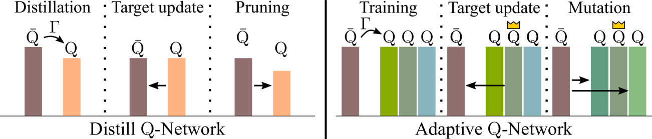
Figure 1: Left: In Distill $Q$-Network, the online network $Q$ is a pruned version of the target network $\bar{Q}$, transforming the classical temporal-difference loss, using the Bellman operator $\Gamma$, into a distillation loss. Right: Adaptive $Q$-Network (Vincent et al., 2025b) uses several online networks, each one defined with different hyperparameters and trained from a shared target network $\bar{Q}$. At each target update, the online network $Q$ with the lowest cumulated loss (represented with a crown) is chosen as the next target network. The target network is then copied to replace the other networks and the hyperparameters of the crowned network are mutated.

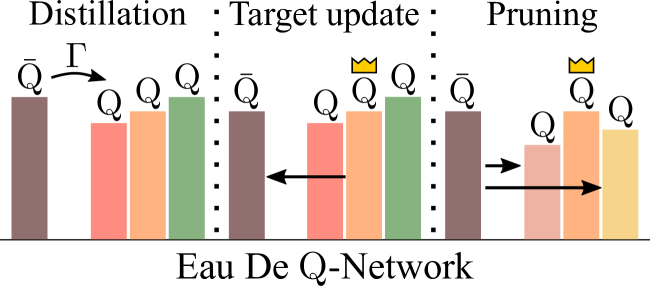
Figure 2: Eau De $Q$-Network is based on Distill $Q$-Network (Figure 1, left) and uses the adaptive ability of Adaptive $Q$-Network (Figure 1, right) to prune the weights of the neural network at the agent’s learning pace.

In this work, we propose a novel approach to sparse training that gradually prunes the weights of the neural networks at the agent’s learning pace to finish at a sparsity level that is discovered by the algorithm. This behavior is made possible thanks to the combination of two independent methods, namely Distill $Q$-Network and Adaptive $Q$-Network (Vincent et al., 2025b), gathered in a single algorithm coined Eau De $Q$-Network (EauDeQN). In Distill $Q$-Network (DistillQN), the online network is a pruned version of the target network, thereby using the common temporal-difference loss as a distillation loss (Figure 1, left). While DistillQN is also a novel approach to sparse training introduced in this work, it still relies on a hand-designed pruning schedule. This is why we will mainly focus on EauDeQN. Adaptive $Q$-Network (AdaQN) was originally introduced to tune the RL agent’s hyperparameters (Vincent et al. (2025b), Figure 1, right). When combined with DistillQN, the resulting algorithm considers several online networks with equal or higher sparsity levels than the target network. At each target update, the online network with the lowest cumulated loss, represented with a crown in Figure 2, is chosen as the next target network. Therefore, the ability to select between different sparsity levels according to the value of the cumulated loss synchronizes the pruning schedule to the agent’s learning pace. The target network is then copied and pruned to replace the other networks. Crucially, by keeping the online network with the lowest cumulated loss for the next iteration, the algorithm can keep the sparsity level steady if the cumulated loss increases for higher sparsity levels. This results in an algorithm capable of discovering the final sparsity level as opposed to the current methods, which rely on a hand-designed sparsity level.

2 Background

Deep $Q$-Network (Mnih et al., 2015)    In a sequential decision-making problem, the optimal action-value function $Q^{*}(s,a)$ is the optimal expected sum of discounted future reward, given a state $s$, an action $a$. From this quantity, the optimal policy $\pi^{*}$ yielding the highest sum of discounted reward can be obtained by directly maximizing $Q^{*}(s,\cdot)$ for a given state $s$. Importantly, the optimal action-value function is the fixed point of the Bellman operator, which is a contraction mapping. The fixed point theorem guarantees that iterating endlessly over any $Q$-function with the Bellman operator converges to the fixed point $Q^{*}$. This is why, to compute $Q^{*}$, Ernst et al. (2005) proposes to learn the successive Bellman iterations using an online network $Q$ and a target network $\bar{Q}$ representing the previous Bellman iteration. The training loss relies on the temporal-difference error, which is defined from a sample $(s,a,r,s^{\prime})$ as

$$\mathcal{L}_{\text{QN}}(Q)=(r+\gamma\max_{a^{\prime}}\bar{Q}(s^{\prime},a^{\prime})-Q(s,a))^{2},$$ (1)

where QN stands for $Q$-Network. After a predefined number of gradient steps, the target network is updated to represent the next Bellman iteration. This procedure repeats until the training ends. Mnih et al. (2015) adapts this framework to the online setting where the agent interacts with the environment using an $\epsilon$-greedy policy (Sutton & Barto, 1998) computed from the online network $Q$.

Adaptive $Q$-Network (Vincent et al., 2025b)    The hyperparameters of DQN are numerous and hard to tune. This is why Vincent et al. (2025b) introduced AdaQN, which is designed to adaptively select DQN’s hyperparameters during training. This is done by considering several online networks trained with different hyperparameters and sharing a single target network. At each target update, the online network with the lowest cumulated loss is selected as the next target network. After each target update, the selected online network is copied to replace the other online networks, and genetic mutations are applied to the hyperparameters of each copy to explore the space of hyperparameters.

3 Related Work

As discussed in Section 1, we focus on dense-to-sparse training methods in this work, as they generally perform better than sparse-to-sparse methods (Graesser et al., 2022). Sparse-to-sparse methods prune a dense network before the training starts (Arnob et al., 2021), relying on the lottery ticket hypothesis (Frankle & Carbin, 2018). The lottery ticket hypothesis makes the assumption that, when initializing a dense network, there exist sub-networks that can lead to similar performances as the dense network if given similar resources. For such methods, the network morphology can still be adapted during training using gradient information (Tan et al., 2023), or evolutionary methods (Sokar et al., 2021; Grooten et al., 2023). On the other hand, dense-to-sparse methods start with a dense network and prune its connections during training. In the machine learning literature, we find approaches using variational dropout to sparsify the network (Molchanov et al., 2017). Alternatively, Liu et al. (2019) design learnable masks by approximating the gradient of the loss function w.r.t. the sparsity level with a piecewise polynomial estimate. Nonetheless, those approaches have not been adapted to an RL setting yet. In the RL literature, Yu et al. (2019) evaluates the lottery ticket hypothesis in an RL setting using a hand-designed geometric sparsity schedule. They conclude that the lottery ticket hypothesis is only valid for a subset of Atari games (Bellemare et al., 2013). Notably, Figure $5$ in Yu et al. (2019) shows that the performances greatly depend on the imposed final sparsity level. Livne & Cohen (2020) makes use of a pre-trained teacher to boost performances. Distillation techniques using pre-trained networks have also been used to kickstart the training in single-task RL settings (Zhang et al., 2019) and multi-task RL settings (Schmitt et al., 2018).

Ceron et al. (2024) is the closest work to our approach. The authors gradually prune the neural network weights during training. They use a polynomial pruning schedule introduced in Zhu & Gupta (2018) and demonstrate that it is effective on the Atari (Bellemare et al., 2013) and MuJoCo (Todorov et al., 2012) benchmarks, yielding even higher performances than the dense counterpart for wide neural networks. As the authors do not give a name to their method, we will refer to it as Polynomial Pruning $Q$-Networks (PolyPruneQN). At any time $t$ during training, a binary mask filtering out the weights with lowest magnitude imposes the sparsity $s_{t}$ to the neural network. $s_{t}$ is defined as

$$s_{t}=s_{F}\left(1-\left(1-\text{Clip}\left(\frac{t-t_{\text{start}}}{t_{\text{end}}-t_{\text{start}}},0,1\right)\right)^{n}\right),$$ (2)

where $s_{F}$ corresponds to the final sparsity level, $t_{\text{start}}$ is the first timestep where the pruning starts, $t_{\text{end}}$ is the timestep after which the sparsity level is kept constant at $s_{F}$, and $n$ controls the steepness of the pruning schedule. One shortcoming of this approach is that those hyperparameters need to be tuned by hand for each RL setting, task, network architecture, and training length.

4 Eau De Q-Network

Our approach uses AdaQN’s adaptivity to learn a pruning schedule synchronized with the agent’s learning pace, therefore avoiding the need to impose a hard-coded sparsity schedule and final sparsity level. For that, we first introduce a novel algorithm called Distill $Q$-Network (DistillQN), which resembles DQN except for the fact that after each target update, the online network is pruned as shown in Figure 1 (left). This algorithm belongs to the dense-to-sparse training family and relies on a hand-designed pruning schedule. We remark that PolyPruneQN is an instance of DistillQN when PolyPruneQN’s pruning period is synchronized with the target update period.

Algorithm 1 Eau De Deep $Q$-Network (EauDeDQN). Modifications to DQN are marked in purple.

1: Initialize $K$ online parameters $(\theta^{k})_{k=1}^{K}$, and an empty replay buffer $\mathcal{D}$. Set $\psi=0$ and $\bar{\theta}\leftarrow\theta^{\psi}$ the target parameters. Set the cumulated losses $L_{k}=0$, for $k=1,\ldots,K$.

2: repeat

3:  Set $\psi^{b}\sim\texttt{Choice}(\{1,..,K\},p=\{\frac{1}{L_{1}},..,\frac{1}{L_{K}}\})$. Illustrated in Figure 3 (right).

4:  Take action $a\sim\epsilon\text{-greedy}(Q_{\theta^{{\color[rgb]{0,0,0}\psi^{b}}}}(s,\cdot))$; Observe reward $r$, next state $s^{\prime}$.

5:  Update $\mathcal{D}\leftarrow\mathcal{D}\bigcup\{(s,a,r,s^{\prime})\}$.

6:  every $G$ steps

7:   Sample a mini-batch $\mathcal{B}=\{(s,a,r,s^{\prime})\}$ from $\mathcal{D}$.

8:   Compute the shared target $y\leftarrow r+\gamma\max_{a^{\prime}}Q_{\bar{\theta}}(s^{\prime},a^{\prime})$.

9:   for $k=1,...,K$ do [in parallel]

10:    Compute the loss w.r.t $\theta^{k}$, $\mathcal{L}^{k}_{\text{QN}}=\sum_{(s,a,r,s^{\prime})\in\mathcal{B}}\left(y-Q_{\theta^{k}}(s,a)\right)^{2}$.

11:    Update $\theta^{k}$ from $\nabla_{\theta^{k}}\mathcal{L}^{k}_{\text{QN}}$ and $L_{k}\leftarrow L_{k}+\mathcal{L}^{k}_{\text{QN}}$.

12:  every $T$ steps

13:   Update the target network $\bar{\theta}\leftarrow\theta^{\psi}$, where $\psi\leftarrow\operatorname*{arg\,min}_{k}L_{k}$.

14:   Exploitation: Select $K$ networks with repetition from the current population using the cumulated losses $L_{k}$. The process is illustrated in Figure 3 (left).

15:   Exploration: Prune the duplicated networks at a sparsity level defined in Equation 3. The process is illustrated in Figure 3 (middle).

16:   Reset $L_{k}\leftarrow 0$, for $k\in\{1,\ldots,K\}$.

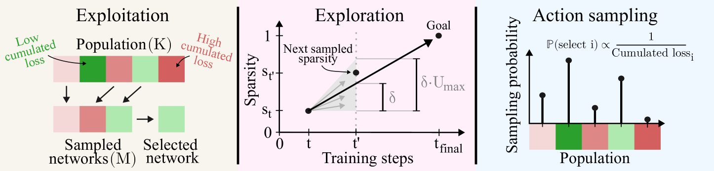
Figure 3: Left: The exploitation phase consists of selecting $K$ networks with repetition from the current population. Each network is selected as the one with the lowest cumulated loss out of $M$ uniformly sampled networks. Middle: In the exploration phase, new sparsity levels are sampled along the line joining the current point $(t,s_{t})$ and the goal $(t_{\text{final}},1)$. To enhance exploration, the obtained sparsity is scaled by $U\sim\mathcal{U}(0,U_{\text{max}})$. Right: At each environment interaction, a network is selected from a probability distribution that is inversely proportional to the cumulated loss.

The combination of DistillQN and AdaQN, which we call Eau De $Q$-Network (EauDeQN), adaptively selects the sparsity level based on the agent’s learning pace. Indeed, EauDeQN considers $K$ online networks with different sparsity levels, each trained against a shared target network. Following the AdaQN algorithm, at each target update, the online network with the lowest cumulated loss is selected as the next target network (see Figure 2). Therefore, at each target update, the online network with the sparsity level that has been the most adapted to the optimization landscape related to the given loss function is selected as the next target network. Before the training continues, the cumulated loss of each online network is used to select the new population of $K$ online networks that will be used to continue the training. Inspired by Miller et al. (1995), and Franke et al. (2021), each member of this new population is selected by randomly sampling $M$ online networks from the $K$ online networks and choosing the one with the lowest cumulated loss as illustrated in Figure 3 (left). One spot in the new population is reserved for the online network chosen as the next target network, i.e., the one with minimal cumulated loss. This is referred to as the exploitation phase in Algorithm 1, Line 14 as it filters out the online networks with a sparsity level that was not well suited for minimizing the current loss function. Then, an exploration phase is responsible for sampling a new sparsity level for each duplicated network. The new sparsity levels chosen at timestep $t$, are kept until timestep $t^{\prime}=t+T$, which corresponds to the timestep of the following target update. We sample each new sparsity level on the line between the current point $(t,s_{t})$ and the goal $(t_{\text{final}},1)$ of reaching a sparsity level of $1$ at the end of the training as illustrated in Figure 3 (middle). This gives the point $(t^{\prime},s_{t}+\delta)$, where $\delta=\frac{1-s_{t}}{t_{\text{final}}-t}(t^{\prime}-t)$. To increase exploration, we scale the obtained sparsity level by $U\sim\mathcal{U}(0,U_{\text{max}})$. Additionally, we ensure that the sampled sparsity level does not remove more than $S_{\text{max}}\times 100\%$ of the remaining parameters such that the jumps in sparsity levels are not too high at the end of the training. This leads to

$$s_{t^{\prime}}=s_{t}+\min\{\underbrace{\frac{1-s_{t}}{t_{\text{final}}-t}(t^{\prime}-t)}_{\text{linear schedule to sparsity of $1$}}\overbrace{U}^{\mathclap{\begin{subarray}{c}\text{stochasticity}\\ \text{injection}\end{subarray}}},\underbrace{(1-s_{t})S_{\text{max}}}_{\text{geometric speed cap}}\},\text{where }U\sim\mathcal{U}(0,U_{\text{max}}).$$ (3)

In practice, setting a sparsity level of $s_{t}$ is done by updating a binary mask over the weights, where the entries corresponding to the $s_{t}\times 100\%$ of the lowest magnitude weights are switched to zero.

Sampling actions are usually performed using an $\epsilon$-greedy policy computed from the online network (Mnih et al., 2015). One could consider using the online network with minimal cumulated loss. However, Vincent et al. (2025b) argue that it is insufficient because the other networks would learn passively, which is detrimental in the long run (Ostrovski et al., 2021). Following the recommendations of Vincent et al. (2025b), we sample an online network from a distribution inversely proportional to the cumulated loss as shown in Figure 3 (right). Then, an $\epsilon$-greedy policy is built on top of this selected network to foster exploration, as described in Line 4 in Algorithm 1.

Overall, this framework is designed to minimize the sum of approximation errors over the training. This motivation is supported by a well-established theoretical result (Theorem $3.4$ from Farahmand (2011)) stating that the sum of approximation errors influences a bound on the performance loss, i.e., the distance between the optimal $Q$-function and the $Q$-function related to the greedy policy obtained at the end of the training. As this property is inherited from AdaQN, we refer to Vincent et al. (2025b) for further details. In the following, we adapted the presented framework to different algorithms. Each time, we append the name of the algorithm with the prefix "EauDe". As an example, EauDeSAC is an instance of EauDeQN applied to Soft Actor-Critic (SAC, Haarnoja et al. (2018)), its pseudo-code is presented in Algorithm 2.

5 Experiments

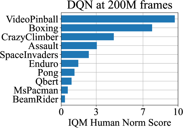
Figure 10: The selected Atari games cover a wide range of normalized returns obtained by DQN after $200$M frames, showcasing their diversity.

We evaluate our approach on $10$ Atari games (Bellemare et al., 2013) and $6$ MuJoCo environments (Todorov et al., 2012). We apply EauDeQN on $3$ different algorithms corresponding to $3$ RL settings. We use DQN (Mnih et al., 2015) in an online scenario, Conservative $Q$-Learning (CQL, Kumar et al. (2020)) in an offline scenario, and SAC (Haarnoja et al., 2018) in an actor-critic setting. In each RL setting, we compare our approach to its dense counterpart and to PolyPruneQN since it is state-of-the-art among pruning methods (Graesser et al., 2022; Ceron et al., 2024). We focus on obtaining returns comparable to those of the dense approach while reaching high final sparsity levels. For that, we report the Inter-Quantile Mean (IQM, Agarwal et al. (2021)) of the normalized return and the sparsity levels along with $95\%$ bootstrapped confidence intervals over $5$ seeds for the Atari games and $10$ seeds for the MuJoCo environments. We believe that the number of samples used during training is the main limiting factor for pruning algorithms. This is why we report the number of environment interactions as the $x$-axis, except for the offline experiments where we report the number of batch updates. We use the hyperparameters shared by Ceron et al. (2024) for PolyPruneQN as they demonstrate that their method is also effective on the considered RL setting, i.e., $s_{F}=0.95,n=3,t_{\text{start}}=0.2\cdot t_{\text{final}},$ and $t_{\text{end}}=0.8\cdot t_{\text{final}},$ where $t_{\text{final}}$ corresponds to the training length. For EauDeQN, we fix $U_{\text{max}}=3,S_{\text{max}}=0.01,K=5$ and $M=3$ and discuss these values in Section 5.4. The shared hyperparameters are kept fixed across the methods and are reported in Table 4 and 4. We reduced the set of $15$ games selected by Ceron et al. (2024) and Graesser et al. (2022) for their diversity to $10$ games to minimize computational costs. Figure 10 testifies that this set of games conserves a wide variety in the magnitude of the normalized return. Details on experiment settings are shared in Section A. The individual learning curves for each environment are presented in the supplementary material.

5.1 Online Q-Learning

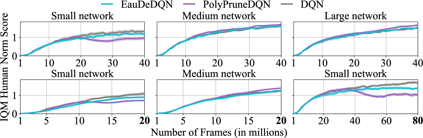
Figure 4: Thanks to its adaptive capability, EauDeDQN performs similarly to its dense counterpart on $10$ Atari games across different network sizes (top row) and training lengths (bottom row). PolyPruneDQN struggles to reach similar returns due to its hard-coded sparsity schedule.

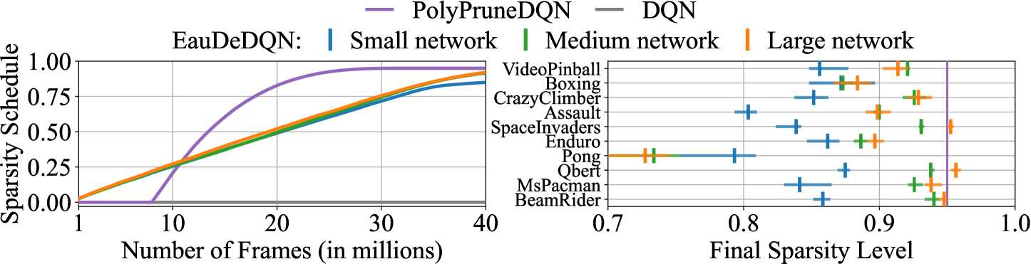
Figure 5: EauDeDQN’s sparsity schedule (left) differs across the $3$ tested network sizes. Higher final sparsity levels are reached for larger network sizes at the end of the training (right), showcasing EauDeDQN’s adaptivity.

We evaluate EauDeDQN’s ability to adapt the sparsity schedule and final sparsity level to different network architectures and training lengths. We make the number of neurons in the first linear layer vary from $32$ (small network) to $512$ (medium network) to $2048$ (large network) while keeping the convolutional layers identical. In Figure 4, EauDeDQN exhibits a stable behavior across the different network sizes (top row) and training lengths (bottom row). EauDeDQN reaches similar performances compared to its dense counterpart as opposed to PolyPruneDQN, which struggles to obtain high returns with a small network architecture.

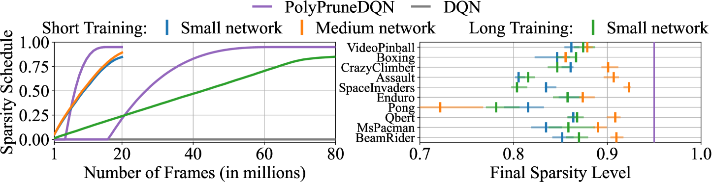
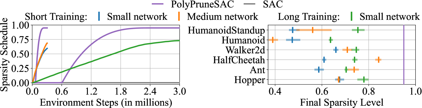
Figure 11: EauDeDQN (top) and EauDeSAC (bottom) adapt the sparsity schedule to the training length. For small networks, increasing the training length leads to higher final sparsity levels (blue and green curves), except for the games Pong, SpaceInvaders, and CrazyClimber. Similarly to Figure 5 and 8, larger networks are pruned at a higher final sparsity level (blue and orange curves), with an exception for Pong and Humanoid.

As the representation capacity of the different network architectures is the same (same convolutional layers), one would desire an adaptive pruning algorithm to prune larger networks more, as compared to smaller networks. Figure 5 (left) shows the sparsity schedule obtained by EauDeDQN along with the hard-coded one of PolyPruneDQN. Interestingly, after following a linear curve, the $3$ EauDeDQN’s sparsity schedules split into $3$ different curves to end at a final sparsity level that is environment-dependent (Figure 5, right). Notably, except for the game Pong, larger final sparsity levels are reached for larger networks, as desired. Figure 11 (top) exhibits similar behaviors where higher final sparsity levels are discovered when more environment interactions are available.

Could the knowledge about the fact that PolyPruneDQN’s medium network performs well with $5\%$ of its weights (Figure 4, middle), be used to tune PolyPruneDQN’s final sparsity level $s_{F}$ for training the small network using the proportion of the network sizes? As the medium network contains $12.4$ times more weights than the small network (see Table 1), the small network should perform well with $62\%$ ($=12.4\times 5\%$) of its weights. This means that one could set $s_{F}$ to $0.38$ ($=1-0.62$) for training the small network. However, even if PolyPruneDQN would achieve good performances at this final sparsity level, it would be significantly lower than the lowest final sparsity level discovered by EauDeDQN ($0.79$ on Pong).

5.2 Offline Q-Learning

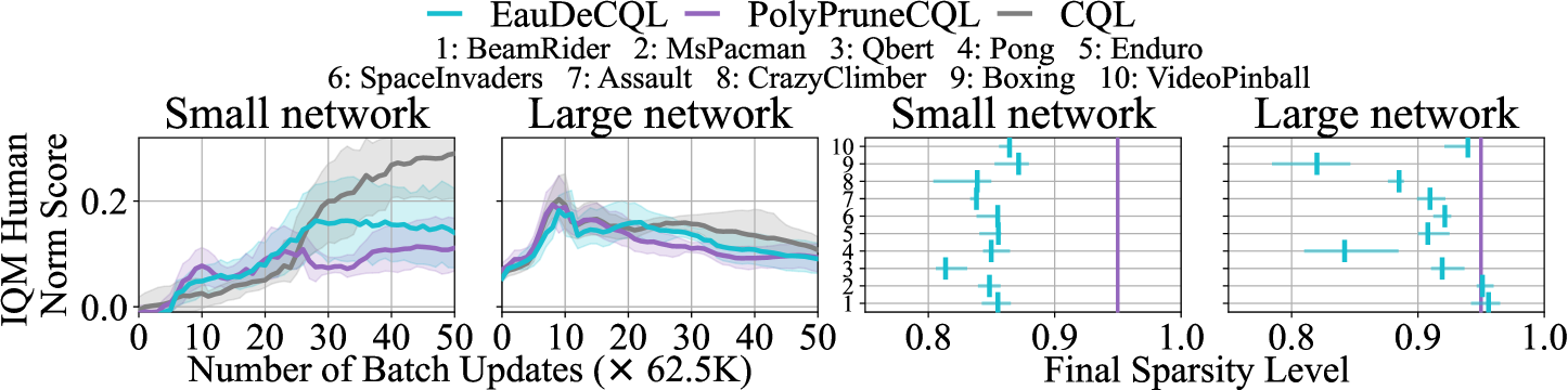
Figure 6: EauDeCQL outperforms PolyPruneCQL when evaluated on $10$ Atari games with a small network and reaches a return similar to the one of CQL with a large network. Importantly, EauDeCQL discovers higher final sparsity levels with a larger network, as desired.

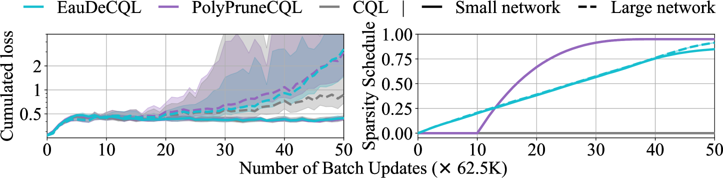
Figure 12: Left: In the offline setting, the larger networks suffer from overfitting as the cumulated losses (reported at every target update and averaged over $T$ updates) increase over time. Right: EauDeCQL adapts the sparsity schedule to the network size. Indeed, sparsity levels are lower for the small network towards the end of the training.

EauDeQN is also designed to work offline as it relies on the cumulated loss to select sparsity levels. Therefore, we evaluate the proposed approach on the same set of $10$ Atari games, using an offline dataset that is composed of $5\%$ of the samples collected by a DQN agent during $200$M environment interactions (Agarwal et al., 2020). In Figure 6 (left), EauDeCQL outperforms PolyPruneCQL for the small network while reaching high sparsity levels, as shown on the right side of the figure. Nonetheless, we note that the confidence intervals overlap and that there is a gap between EauDeCQL and CQL performances. For the larger network, all algorithms reach similar return, with slowly decreasing return over time, as also observed in Ceron et al. (2024). We attribute this behavior to overfitting as the cumulated losses increase over time (see Figure 12, left). Notably, the sparsity levels reached by EauDeCQL are higher for the larger network, as desired (see Figure 6).

5.3 Actor-Critic Method

We verify that the proposed framework can be used in an actor-critic setting. Similarly to the online Atari experiments in Section 5.1, we observe in Figure 7 a stable behavior of EauDeSAC, which yields comparable performances to SAC when the network architecture and the training length vary. On the other hand, PolyPruneSAC suffers when evaluated on small network sizes. The small network corresponds to the commonly used architecture ($256$ neurons for each of the $2$ linear layers (Haarnoja et al., 2018)), the number of neurons per layer is scaled by $5$ for the medium network and by $8$ for the large network. As a sanity check, we verified that the final sparsity levels discovered by EauDeSAC can also be used by PolyPruneSAC to achieve high returns. In Figure 7 (bottom), PolyPruneSAC (oracle) validates this hypothesis by reaching similar performances as SAC and EauDeSAC.

Figure 8 shows the sparsity schedules (left) that lead to the final sparsity levels (right). This time, the difference between the $3$ sparsity schedules of EauDeSAC is even more pronounced than for the online Atari experiments. This can be explained by the fact that the differences in scale between the networks are larger than for the Atari experiments (see Table 1). Indeed, the small network is $18.8$ times smaller than the medium network and $46.6$ times smaller than the large network. By adaptively selecting the network with the lowest cumulated loss, EauDeSAC filters out the networks with sparsity levels that are too high to fit the regression target. This is why the curve of EauDeSAC’s sparsity schedule for the small network is lower than for the larger networks (except for the Humanoid environment). Similar conclusions can be drawn for the sparsity schedules obtained with varying training lengths (see Figure 11, bottom).

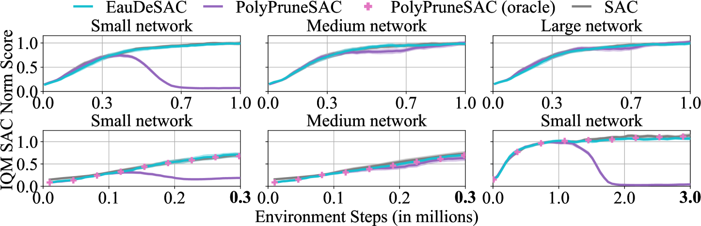
Figure 7: Thanks to its adaptive capability, EauDeSAC performs similarly to its dense counterpart on $6$ MuJoCo games across different network sizes (top row) and training lengths (bottom row). PolyPruneSAC struggles to reach similar returns due to its hard-coded sparsity schedule. PolyPruneSAC (oracle) performs well when the final sparsity is set to the value discovered by EauDeSAC.

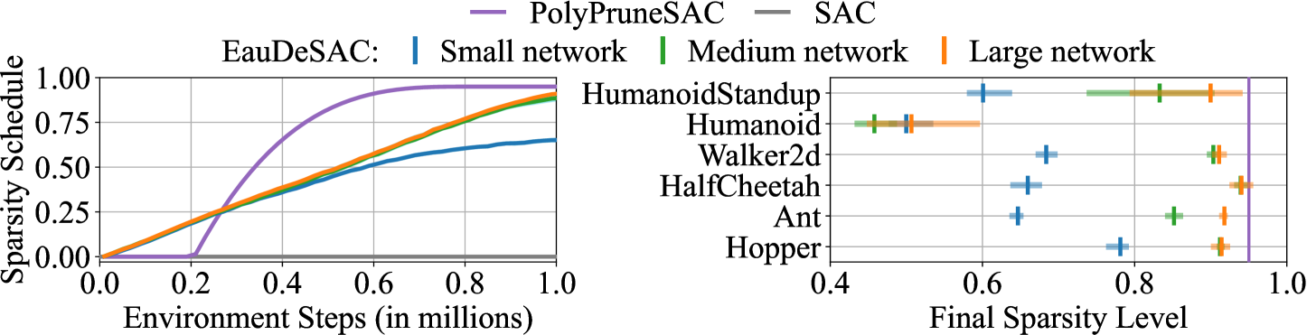
Figure 8: EauDeSAC’s sparsity schedule (left) differs across the $3$ tested network sizes. Higher final sparsity levels are reached for larger network sizes at the end of the training (right), showcasing EauDeSAC’s adaptivity.

Knowing that PolyPruneSAC’s medium network performs well with $5\%$ of its weights can also not be used to tune PolyPruneSAC’s final sparsity level for the small network. Indeed, the medium network is $18.8$ times smaller than the small network. This means that the small network could perform well with $94\%$ ($=18.8\times 5\%$) of its weights. This leads to a final sparsity level for PolyPruneSAC of $0.06$ ($=1-0.94$), which is significantly lower than the lowest sparsity level discovered by EauDeSAC ($0.5$ for Humanoid).

5.4 Ablation Study

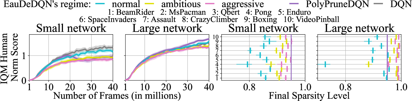
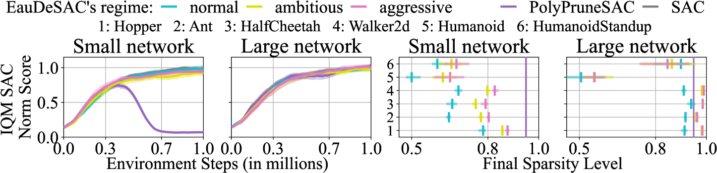
Figure 9: Evaluation of EauDeDQN on $10$ Atari games (top) and EauDeSAC on $6$ MuJoCo environments (bottom) demonstrating that the tradeoff between high return and high sparsity can be tuned using $U_{\text{max}}$. For higher values of $U_{\text{max}}$ (more aggressive regimes), EauDeQN reaches higher final sparsity levels at the cost of a lower return.

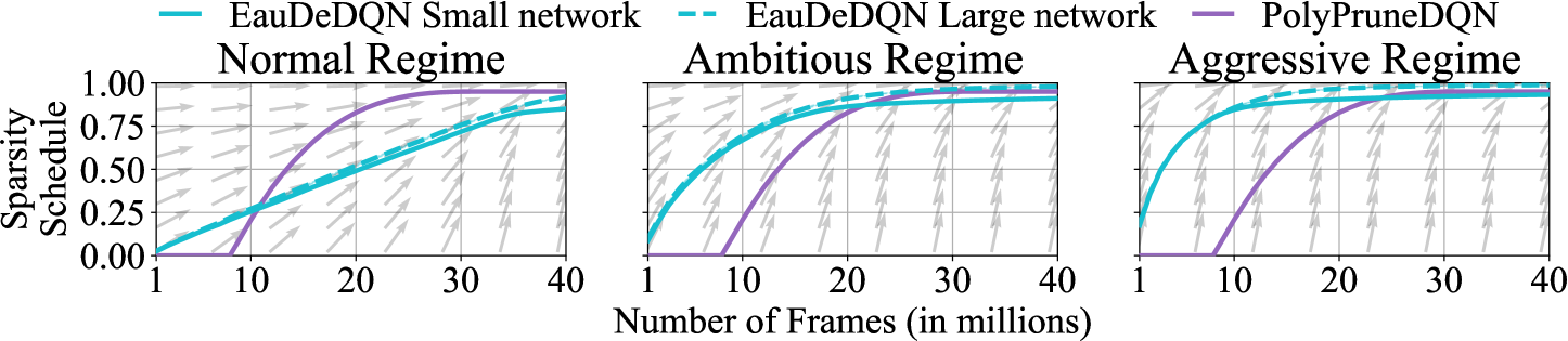
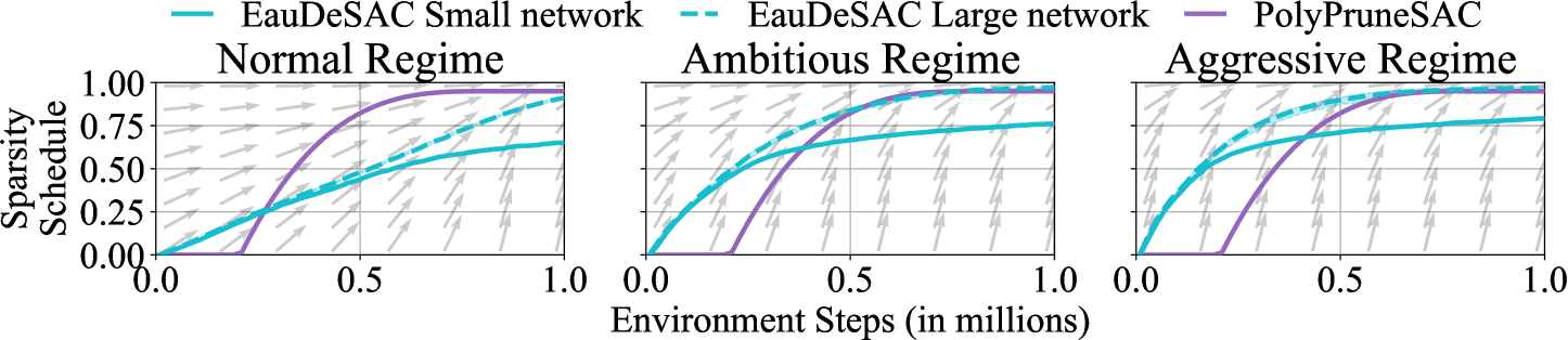
Figure 14: Sparsity schedules of EauDeDQN on $10$ Atari games (top) and EauDeSAC on $6$ MuJoCo environments (bottom) for different regimes: normal ($U_{\text{max}}=3$), ambitious ($U_{\text{max}}=10$), and aggressive ($U_{\text{max}}=30$). The vector fields in the background show the average direction from which the new sparsities are sampled, similar to Figure 3 (middle). As desired, larger networks tend to reach higher sparsity levels. Remarkably, the sparsity levels of the ambitious and aggressive regimes for the large network surpass PolyPruneQN sparsity levels, obtaining higher final sparsity levels while keeping performances high (see Figure 9).

We now study the sensitivity of EauDeQN to the exploration hyperparameter $U_{\text{max}}$ introduced in Equation 3. For that, in Figure 9, we evaluate EauDeDQN (top row) and EauDeSAC (bottom row) with small and large networks, setting $U_{\text{max}}$ to $3,10,$ and $30$. This results in a normal, ambitious, and aggressive regime respectively. On both benchmarks, we observe that this hyperparameter offers a tradeoff between high return and high sparsity. As expected, more aggressive regimes constantly yield higher final sparsity levels as higher values of $U_{\text{max}}$ lead to higher values of sampled sparsity. Across all regimes, we recover the property identified earlier that the final sparsity level for the small networks is lower than for the large network. Figure 14 confirms this behavior by showing the sparsity schedules obtained by EauDeDQN (top row) and EauDeSAC (bottom row). Remarkably, with the large network, the aggressive regime reaches final sparsity levels higher than $0.95$ while keeping high performances. We also observe that the aggressive regime is less well suited for the small network on the Atari experiments. Therefore, we recommend increasing the aggressivity of the regime with the network size. In Figure 13 (left), we compare the Pareto front between sparsity and return of EauDeSAC and PolyPruneSAC. We conclude that EauDeSAC’s regime parameter ($U_{\text{max}}$) is easier to tune as setting it too high does not lead to poor performances as opposed to setting PolyPruneSAC’s final sparsity level at a high value. Finally, Figure 13 (right) presents another ablation study on $2$ other hyperparameters ($S_{\text{max}}$ and the population size $K$) showing that EauDeSAC’s performance remains stable for a wide range of hyperparameter values.

6 Conclusion and Limitations

We introduced EauDeQN, an algorithm capable of pruning the neural networks’ weights at the agent’s learning pace. As opposed to current approaches, the final level of sparsity is discovered by the algorithm. These capabilities are achieved by combining DistillQN (also introduced in this work) with AdaQN (Vincent et al., 2025b). We demonstrated that EauDeQN yields high final sparsity levels while keeping performances close to its dense counterpart in a wide variety of problems.

Limitations Similarly to AdaQN, EauDeQN requires additional time and memory during training. This is a usual drawback of dense-to-sparse approaches (Graesser et al., 2022). Nonetheless, those additional requirements remain reasonable as quantified in Table 2. Another limitation of our work concerns the actor-critic framework. Our algorithm focuses on pruning the critic only. Nonetheless, it is usually the network of the critic that requires a larger amount of parameters (Zhou et al., 2020; Kostrikov et al., 2021; Graesser et al., 2022; Bhatt et al., 2024). Future work could investigate pruning the actor with a simple hand-designed pruning schedule, as done in Xu et al. (2024), while using EauDeQN to prune the critic.

Appendix A Appendix

Our codebase is written in Jax (Bradbury et al., 2018) and relies on JaxPruner (Lee et al., 2024). The code is available in the supplementary material and will be made open source upon acceptance. After each exploration step of EauDeQN, we reset the optimizer of the duplicated networks, as advocated by Asadi et al. (2023), while leaving the optimizer of the other networks intact, similarly to PolyPruneQN.

Atari experiment. We build our codebase on Vincent et al. (2025a) implementation which follows Castro et al. (2018) standards. Those standards are detailed in Machado et al. (2018). Namely, we use the game over signal to terminate an episode instead of the life signal. The input given to the neural network is a concatenation of $4$ frames in grayscale of dimension $84$ by $84$. To get a new frame, we sample $4$ frames from the Gym environment (Brockman et al., 2016) configured with no frame-skip, and we apply a max pooling operation on the $2$ last grayscale frames. We use sticky actions to make the environment stochastic (with $p=0.25$). The reported performance is the one obtained during training.

MuJoCo experiment. We build PolyPruneSAC and EauDeSAC on top of SBX (Raffin et al., 2021). The agent is evaluated every $10$k environment interaction. While Ceron et al. (2024) apply the hand-designed sparsity schedule on the actor and the critic, in this work, we only prune the critic for PolyPruneSAC and EauDeSAC to remain aligned with the theoretical motivation behind EauDeQN and AdaQN (Vincent et al., 2025b).

Table 1: Number of parameters of the different network sizes and scaling factor compared to the small network (in parenthesis). Computations were made on the game SpaceInvaders and on Ant.

	Small network	Medium network	Large network
Atari	$326\,022$	$4\,046\,502$ ($\times 12.4$)	$15\,952\,038$ ($\times 48.9$)
MuJoCo	$94\,984$	$1\,785\,608$ ($\times 18.8$)	$4\,429\,832$ ($\times 46.6)$

Table 2: While EauDeQN requires additional resources compared to PolyPruneQN, it avoids the need to tune the final sparsity level, which in turn saves resources. Computations are reported for the medium network for every algorithm.

	EauDeDQN	EauDeCQL	EauDeSAC
	vs PolyPruneDQN	vs PolyPruneCQL	vs PolyPruneSAC
Training time	$\times 1,39$	$\times 1,17$	$\times 1,08$
GPU vRAM usage	$+0,73$ Gb	$+0,65$ Gb	$+0,01$ Gb
FLOPs for a gradient update	$\times 1.55$	$\times 1.55$	$\times 4.03$
FLOPs for sampling an action	$\times 1.01$	(offline)	$\times 1.00$

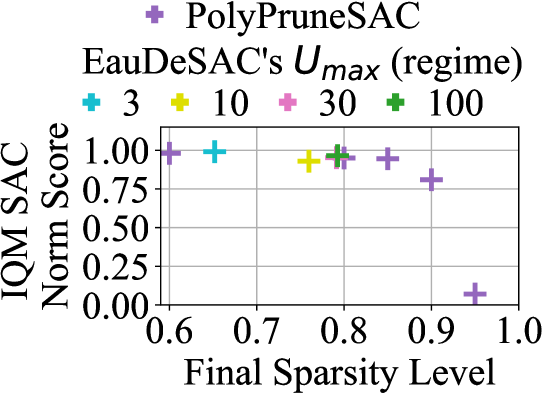
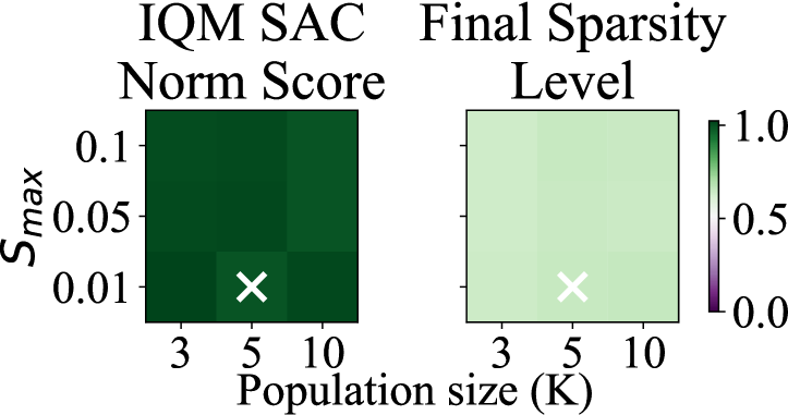
Figure 13: We evaluate EauDeSAC on $6$ MuJoCo environments for $1$M with the small network. Left: PolyPruneSAC suffers when its final sparsity level is too high as opposed to EauDeSAC, which yields high returns for all considered values of $U_{\text{max}}$. Right: EauDeSAC remains stable across different values of $S_{\text{max}}$ and population size $K$ (see Equation 3), showcasing its robustness w.r.t. hyperparameter changes. The number of subsampled networks $M$ is set to $\left\lceil\frac{K}{2}\right\rceil$. The default hyperparameters of EauDeQN are indicated with a white cross.

Algorithm 2 Eau De Soft Actor-Critic (EauDeSAC). Modifications to SAC are marked in purple.

1: Initialize the policy parameters $\phi$, $2$ $\cdot K$ online parameters $(\theta_{i}^{k})_{k=1}^{K}$, for $i\in\{1,2\}$, and an empty replay buffer $\mathcal{D}$. For $k=1,..,K$ and $i\in\{1,2\}$, set the target parameters $\bar{\theta}_{i}^{k}\leftarrow\theta_{i}^{k}$, and the cumulated losses $L_{i}^{k}=0$. Set $\psi_{1}=\psi_{2}=0$ the indices to be selected for computing the target.

2: repeat

3:  Take action $a\sim\pi_{\phi}(\cdot|s)$; Observe reward $r$, next state $s^{\prime}$; $\mathcal{D}\leftarrow\mathcal{D}\bigcup\{(s,a,r,s^{\prime})\}$.

4:  for UTD updates do

5:   Sample a mini-batch $\mathcal{B}=\{(s,a,r,s^{\prime})\}$ from $\mathcal{D}$.

6:   Compute the shared target

$$y\leftarrow r+\gamma\left(\min_{\bar{\theta}\in\left\{\bar{\theta}_{1}^{{\color[rgb]{0,0,0}\psi_{1}}},\bar{\theta}_{2}^{{\color[rgb]{0,0,0}\psi_{2}}}\right\}}Q_{\bar{\theta}}(s^{\prime},a^{\prime})-\alpha\log\pi_{\phi}(a^{\prime}|s^{\prime})\right),\text{where }a^{\prime}\sim\pi_{\phi}(\cdot|s^{\prime}).$$

7:   for $k=1,..,K$ and $i=1,2$ do [in parallel]

8:    Compute the loss w.r.t $\theta_{i}^{k}$, $\mathcal{L}^{k,i}_{\text{QN}}=\sum_{(s,a,r,s^{\prime})\in\mathcal{B}}\left(y-Q_{\theta_{i}^{k}}(s,a)\right)^{2}$.

9:    Update $\theta_{i}^{k}$ from $\nabla_{\theta_{i}^{k}}\mathcal{L}^{k,i}_{\text{QN}}$, $\bar{\theta}_{i}^{k}\leftarrow\tau\theta_{i}^{k}+(1-\tau)\bar{\theta}_{i}^{k}$, and $L_{i}^{k}\leftarrow(1-\tau)L_{i}^{k}+\tau\mathcal{L}^{k,i}_{\text{QN}}$.

10:   Set $\psi_{i}\leftarrow\operatorname*{arg\,min}_{k}L_{i}^{k}$, for $i\in\{1,2\}$.

11:  Set $\psi_{i}^{b}\sim\texttt{Choice}(\{1,..,K\},p=\{\frac{1}{L_{i}^{1}},..,\frac{1}{L_{i}^{K}}\})$, for $i\in\{1,2\}$.

12:  Update $\phi$ with gradient ascent using the loss

$$\min_{\theta\in\left\{\theta_{1}^{{\color[rgb]{0,0,0}\psi_{1}^{b}}},\theta_{2}^{{\color[rgb]{0,0,0}\psi_{2}^{b}}}\right\}}Q_{\theta}(s,a)-\alpha\log\pi_{\phi}(a|s),~~a\sim\pi_{\phi}(\cdot|s)$$

13:  every $P$ steps

14:   Exploitation: Select $K$ networks with repetition from the current population using the cumulated losses $L_{i}^{k}$. The process is illustrated in Figure 3 (left).

15:   Exploration: Prune the duplicated networks at a sparsity level defined in Equation 3. The process is illustrated in Figure 3 (middle).

16:   Reset $L_{i}^{k}\leftarrow 0$, for $k\in\{1,\ldots,K\}$ and $i\in\{1,2\}$.

Supplementary Materials
The following content was not necessarily subject to peer review.

 

Figure 15: Online Atari: Per game metrics for the experiment on the small network. The aggregated performances are available in Figure 4 (top, left).

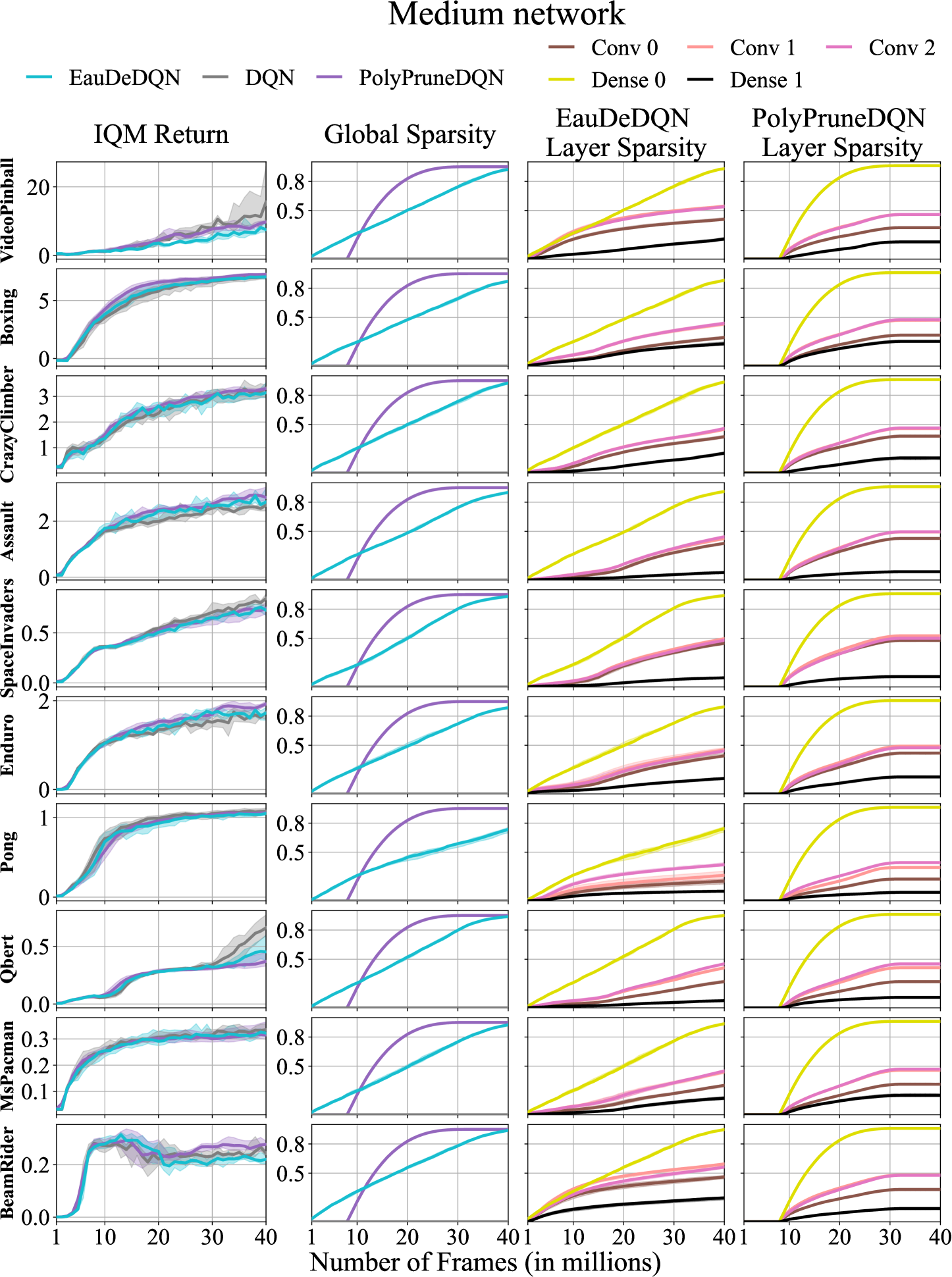
Figure 16: Online Atari: Per game metrics for the experiment on the medium network. The aggregated performances are available in Figure 4 (top, middle).

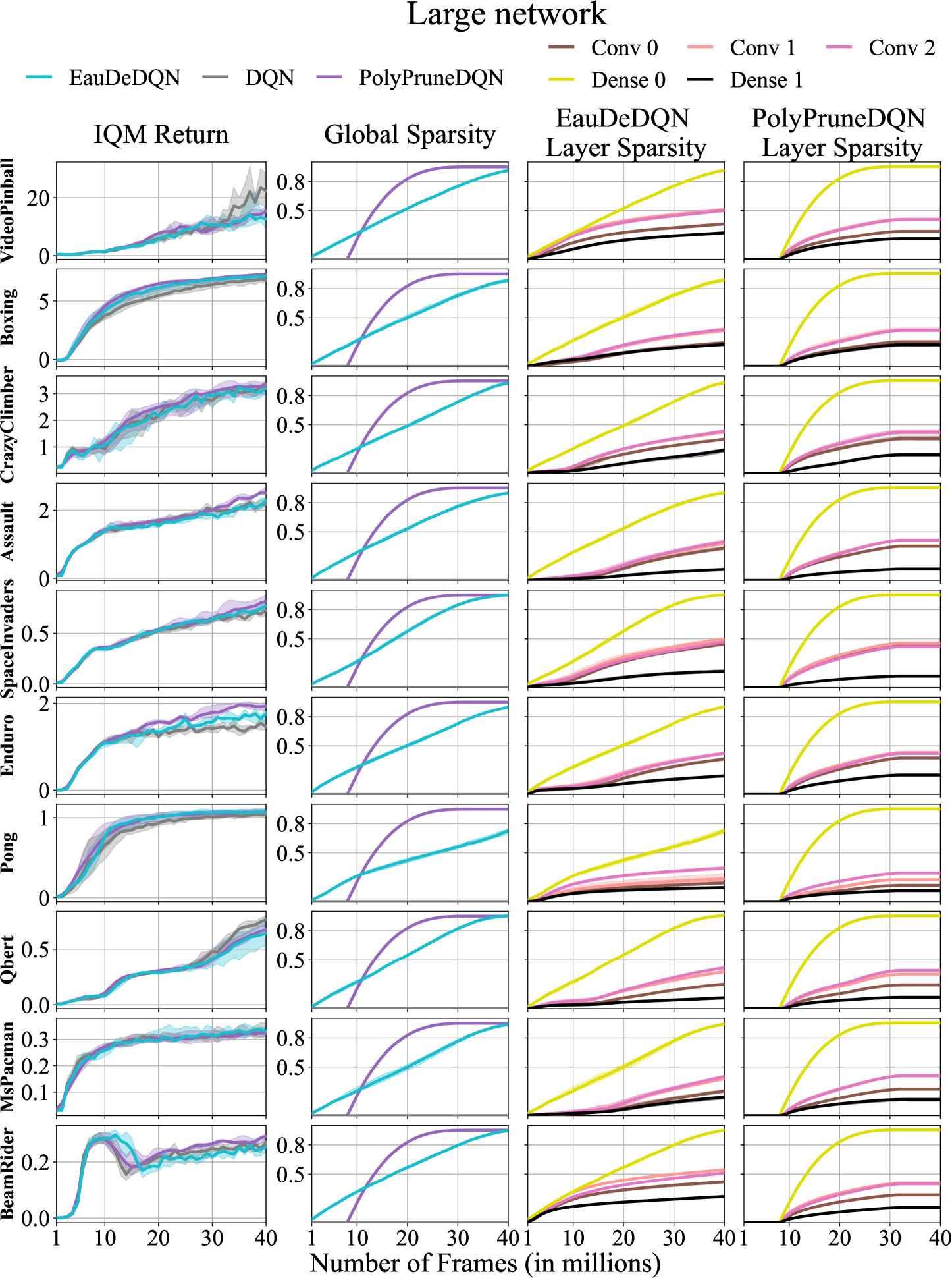
Figure 17: Online Atari: Per game metrics for the experiment on the large network. The aggregated performances are available in Figure 4 (top, right).

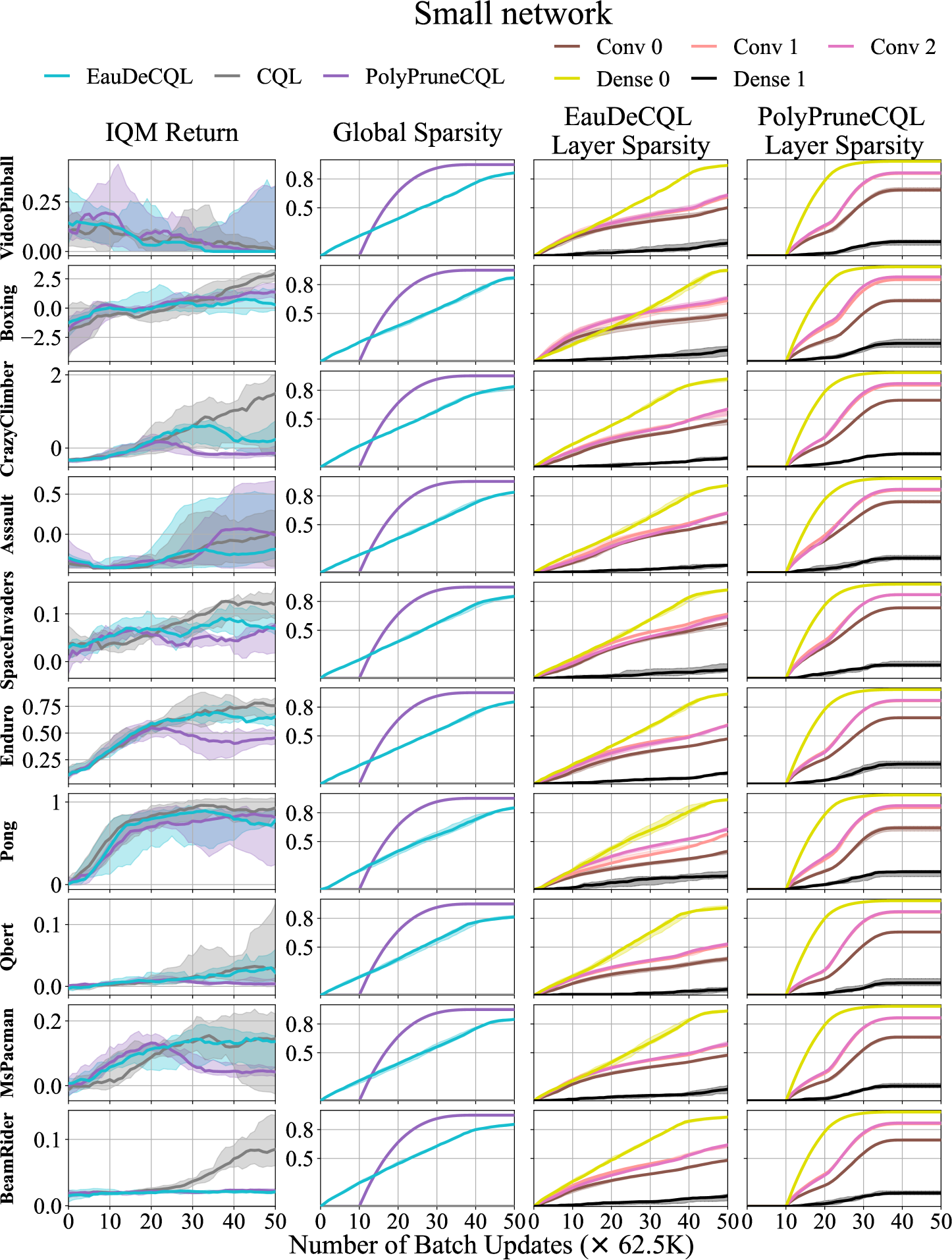
Figure 18: Offline Atari: Per game metrics for the experiment on the small network. The aggregated performances are available in Figure 6 ($1^{\text{st}}$ plot to the left).

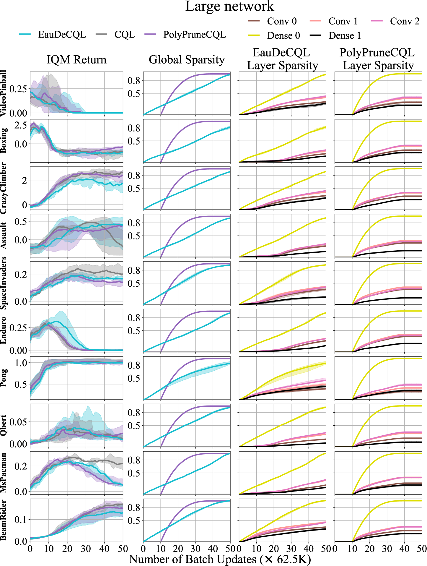
Figure 19: Offline Atari: Per game metrics for the experiment on the large network. The aggregated performances are available in Figure 6 ($2^{\text{nd}}$ plot to the left).

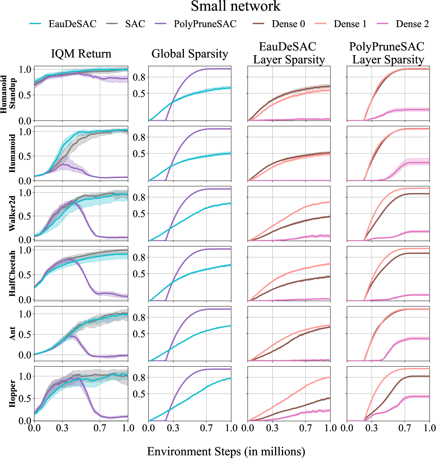
Figure 20: Online MuJoCo: Per game metrics for the experiment on the small network. The aggregated performances are available in Figure 7 (top, left).

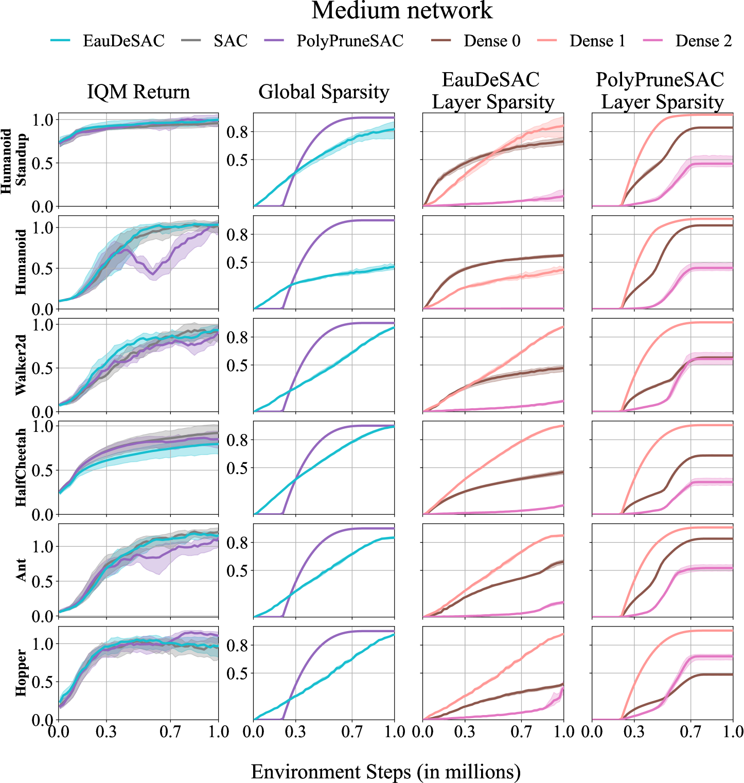
Figure 21: Online MuJoCo: Per game metrics for the experiment on the medium network. The aggregated performances are available in Figure 7 (top, middle).

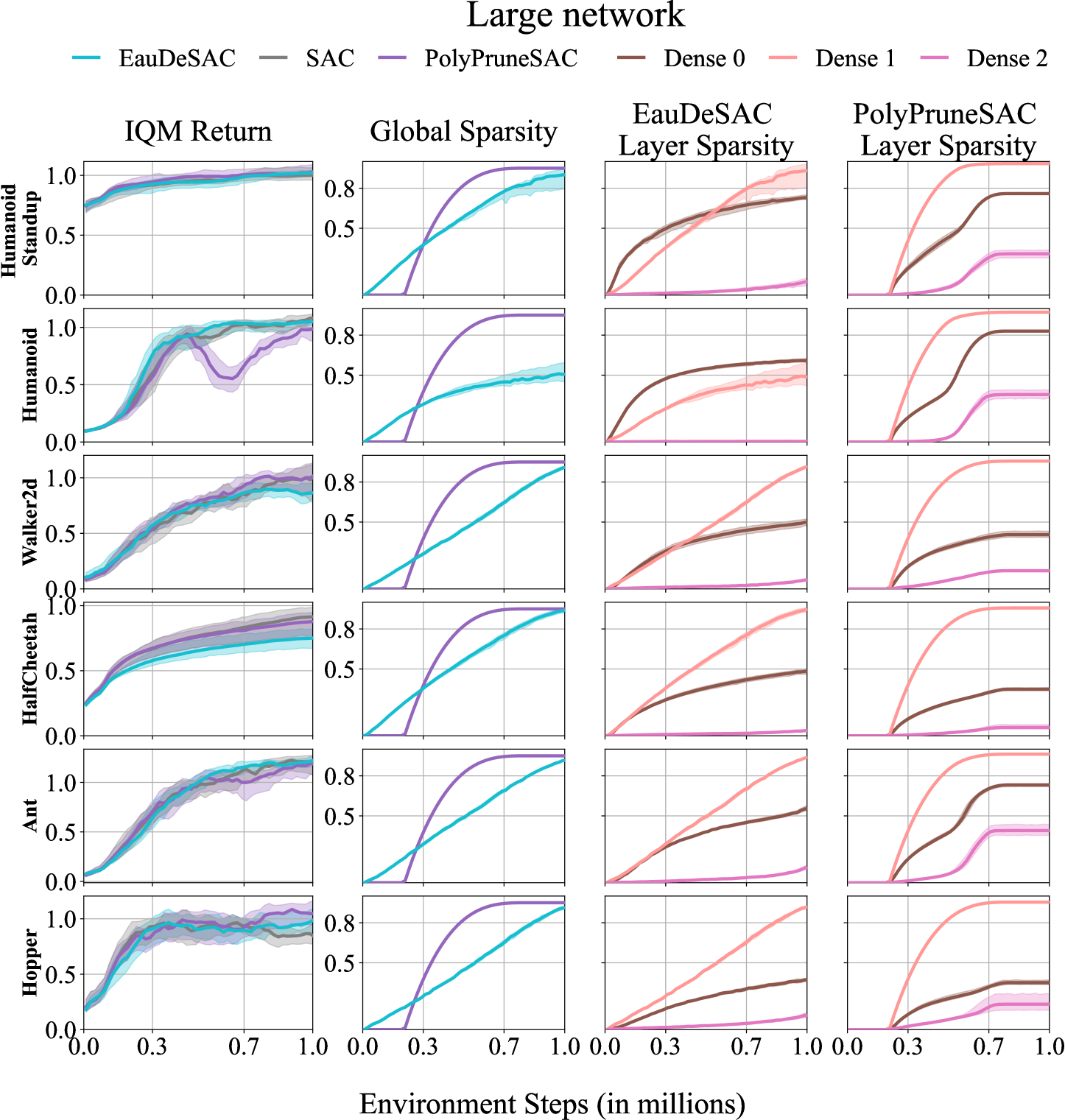
Figure 22: Online MuJoCo: Per game metrics for the experiment on the large network. The aggregated performances are available in Figure 7 (top, right).

Table 3: Summary of the shared hyperparameters used for the Atari experiments. We note $\text{Conv}_{a,b}^{d}C$ a $2D$ convolutional layer with $C$ filters of size $a\times b$ and of stride $d$, and $\text{FC }E$ a fully connected layer with $E$ neurons.

Environment
Discount factor $\gamma$	$0.99$
Horizon $H$	$27\,000$
Full action space	No
Reward clipping	clip($-1,1$)
All experiments
Batch size	$32$
Torso architecture	$\text{Conv}_{8,8}^{4}32$
	$-\text{Conv}_{4,4}^{2}64$
	$-\text{Conv}_{3,3}^{1}64$
Head architecture	$\text{FC }32$ (small)
	$\text{FC }512$ (medium)
	$\text{FC }2048$ (large)
	$-\text{FC }n_{\mathcal{A}}$
Activations	ReLU
PolyPruneQN	$4\,000$ (online)
pruning period	$1\,000$ (offline)
Online experiments
Number of training	$250\,000$
steps per epochs
Target update	$8\,000$
period $T$
Type of the	FIFO
replay buffer $\mathcal{D}$
Initial number	$20\,000$
of samples in $\mathcal{D}$
Maximum number	$1\,000\,000$
of samples in $\mathcal{D}$
Gradient step	$4$
period $G$
Starting $\epsilon$	$1$
Ending $\epsilon$	$0.01$
$\epsilon$ linear decay	$250\,000$
duration
Batch size	$32$
Learning rate	$6.25\times 10^{-5}$
Adam $\epsilon$	$1.5\times 10^{-4}$
Offline experiments
Number of training	$62\,500$
steps per epochs
Target update	$2\,000$
period $T$
Dataset size	$2\,500\,000$
Learning rate	$5\times 10^{-5}$
Adam $\epsilon$	$3.125\times 10^{-4}$

Table 4: Summary of all hyperparameters used for the MuJoCo experiments. We note $\text{FC }E$ a fully connected layer with $E$ neurons.

Environment
Discount factor $\gamma$	$0.99$
Horizon $H$	$1\,000$
All algorithms
Number of	$1\,000\,000$
training steps
Type of the	FIFO
replay buffer $\mathcal{D}$
Initial number	$5\,000$
of samples in $\mathcal{D}$
Maximum number	$1\,000\,000$
of samples in $\mathcal{D}$
Update-To-Data	$1$
UTD
Batch size	$256$
Learning rate	$10^{-3}$
Policy delay	$1$
Actor architecture	$\text{FC }256$
	$-\text{FC }256$
Critic architecture	$\text{FC }256$
	$-\text{FC }256$ (small)
	$\text{FC }1280$
	$-\text{FC }1280$ (medium)
	$\text{FC }2048$
	$-\text{FC }2048$ (large)
Soft target update	$5\times 10^{-3}$
period $\tau$
Pruning period $P$	$1\,000$

References

- Agarwal et al. (2020) Rishabh Agarwal, Dale Schuurmans, and Mohammad Norouzi. An optimistic perspective on offline reinforcement learning. In International Conference on Machine Learning, 2020.
- Agarwal et al. (2021) Rishabh Agarwal, Max Schwarzer, Pablo Samuel Castro, Aaron Courville, and Marc Bellemare. Deep reinforcement learning at the edge of the statistical precipice. In Advances in Neural Information Processing Systems, 2021.
- Arnob et al. (2021) Samin Yeasar Arnob, Riyasat Ohib, Sergey Plis, and Doina Precup. Single-shot pruning for offline reinforcement learning. Neurips Workshop on Offline Reinforcement Learning, 2021.
- Asadi et al. (2023) Kavosh Asadi, Rasool Fakoor, and Shoham Sabach. Resetting the optimizer in deep RL: An empirical study. In Advances in Neural Information Processing Systems, 2023.
- Bellemare et al. (2013) Marc G Bellemare, Yavar Naddaf, Joel Veness, and Michael Bowling. The arcade learning environment: An evaluation platform for general agents. Journal of Artificial Intelligence Research, 2013.
- Bhatt et al. (2024) Aditya Bhatt, Daniel Palenicek, Boris Belousov, Max Argus, Artemij Amiranashvili, Thomas Brox, and Jan Peters. Crossq: Batch normalization in deep reinforcement learning for greater sample efficiency and simplicity. International Conference on Learning Representations, 2024.
- Bradbury et al. (2018) James Bradbury, Roy Frostig, Peter Hawkins, Matthew James Johnson, Chris Leary, Dougal Maclaurin, George Necula, Adam Paszke, Jake VanderPlas, Skye Wanderman-Milne, and Qiao Zhang. JAX: composable transformations of Python+NumPy programs, 2018.
- Brockman et al. (2016) Greg Brockman, Vicki Cheung, Ludwig Pettersson, Jonas Schneider, John Schulman, Jie Tang, and Wojciech Zaremba. Openai gym. arXiv preprint arXiv:1606.01540, 2016.
- Castro et al. (2018) Pablo Samuel Castro, Subhodeep Moitra, Carles Gelada, Saurabh Kumar, and Marc G Bellemare. Dopamine: A research framework for deep reinforcement learning. arXiv preprint arXiv:1812.06110, 2018.
- Ceron et al. (2024) Johan Samir Obando Ceron, Aaron Courville, and Pablo Samuel Castro. In value-based deep reinforcement learning, a pruned network is a good network. In International Conference on Machine Learning, 2024.
- Ernst et al. (2005) Damien Ernst, Pierre Geurts, and Louis Wehenkel. Tree-based batch mode reinforcement learning. Journal of Machine Learning Research, 2005.
- Espeholt et al. (2018) Lasse Espeholt, Hubert Soyer, Remi Munos, Karen Simonyan, Vlad Mnih, Tom Ward, Yotam Doron, Vlad Firoiu, Tim Harley, Iain Dunning, et al. Impala: Scalable distributed deep-rl with importance weighted actor-learner architectures. In International Conference on Machine Learning, 2018.
- Evci et al. (2019) Utku Evci, Fabian Pedregosa, Aidan Gomez, and Erich Elsen. The difficulty of training sparse neural networks. In ICML Workshop on Identifying and Understanding Deep Learning Phenomena, 2019.
- Evci et al. (2020) Utku Evci, Trevor Gale, Jacob Menick, Pablo Samuel Castro, and Erich Elsen. Rigging the lottery: Making all tickets winners. In International Conference on Machine Learning, 2020.
- Farahmand (2011) Amir-massoud Farahmand. Regularization in reinforcement learning. PhD thesis, University of Alberta, 2011.
- Franke et al. (2021) Jörg KH Franke, Gregor Koehler, André Biedenkapp, and Frank Hutter. Sample-efficient automated deep reinforcement learning. In International Conference on Learning Representations, 2021.
- Frankle & Carbin (2018) Jonathan Frankle and Michael Carbin. The lottery ticket hypothesis: Finding sparse, trainable neural networks. In International Conference on Learning Representations, 2018.
- Graesser et al. (2022) Laura Graesser, Utku Evci, Erich Elsen, and Pablo Samuel Castro. The state of sparse training in deep reinforcement learning. In International Conference on Machine Learning, 2022.
- Grooten et al. (2023) Bram Grooten, Ghada Sokar, Shibhansh Dohare, Elena Mocanu, Matthew E Taylor, Mykola Pechenizkiy, and Decebal Constantin Mocanu. Automatic noise filtering with dynamic sparse training in deep reinforcement learning. In International Conference on Autonomous Agents and Multiagent System, 2023.
- Haarnoja et al. (2018) Tuomas Haarnoja, Aurick Zhou, Pieter Abbeel, and Sergey Levine. Soft actor-critic: Off-policy maximum entropy deep reinforcement learning with a stochastic actor. In International Conference on Machine Learning, 2018.
- Han et al. (2015) Song Han, Huizi Mao, and William J Dally. Deep compression: Compressing deep neural networks with pruning, trained quantization and huffman coding. International Conference on Learning Representations, 2015.
- Henderson et al. (2018) Peter Henderson, Riashat Islam, Philip Bachman, Joelle Pineau, Doina Precup, and David Meger. Deep reinforcement learning that matters. In Association for the Advancement of Artificial Intelligence, 2018.
- Kostrikov et al. (2021) Ilya Kostrikov, Rob Fergus, Jonathan Tompson, and Ofir Nachum. Offline reinforcement learning with fisher divergence critic regularization. In International Conference on Machine Learning, 2021.
- Kumar et al. (2020) Aviral Kumar, Aurick Zhou, George Tucker, and Sergey Levine. Conservative q-learning for offline reinforcement learning. Advances in Neural Information Processing Systems, 2020.
- Lee et al. (2024) Joo Hyung Lee, Wonpyo Park, Nicole Elyse Mitchell, Jonathan Pilault, Johan Samir Obando Ceron, Han-Byul Kim, Namhoon Lee, Elias Frantar, Yun Long, Amir Yazdanbakhsh, et al. Jaxpruner: A concise library for sparsity research. In Conference on Parsimony and Learning, 2024.
- Liu et al. (2020) Junjie Liu, Zhe Xu, Runbin Shi, Ray CC Cheung, and Hayden KH So. Dynamic sparse training: Find efficient sparse network from scratch with trainable masked layers. International Conference on Learning Representations, 2020.
- Liu et al. (2019) Zhuang Liu, Mingjie Sun, Tinghui Zhou, Gao Huang, and Trevor Darrell. Rethinking the value of network pruning. In International Conference on Learning Representations, 2019.
- Livne & Cohen (2020) Dor Livne and Kobi Cohen. Pops: Policy pruning and shrinking for deep reinforcement learning. IEEE Journal of Selected Topics in Signal Processing, 2020.
- Machado et al. (2018) Marlos C Machado, Marc G Bellemare, Erik Talvitie, Joel Veness, Matthew Hausknecht, and Michael Bowling. Revisiting the arcade learning environment: Evaluation protocols and open problems for general agents. Journal of Artificial Intelligence Research, 2018.
- Miller et al. (1995) Brad L Miller, David E Goldberg, et al. Genetic algorithms, tournament selection, and the effects of noise. Complex systems, 1995.
- Mnih et al. (2015) Volodymyr Mnih, Koray Kavukcuoglu, David Silver, Andrei A Rusu, Joel Veness, Marc G Bellemare, Alex Graves, Martin Riedmiller, Andreas K Fidjeland, Georg Ostrovski, et al. Human-level control through deep reinforcement learning. Nature, 2015.
- Mocanu et al. (2018) Decebal Constantin Mocanu, Elena Mocanu, Peter Stone, Phuong H Nguyen, Madeleine Gibescu, and Antonio Liotta. Scalable training of artificial neural networks with adaptive sparse connectivity inspired by network science. Nature Communications, 2018.
- Molchanov et al. (2017) Dmitry Molchanov, Arsenii Ashukha, and Dmitry Vetrov. Variational dropout sparsifies deep neural networks. In International Conference on Machine Learning, 2017.
- Nauman et al. (2024) Michal Nauman, Mateusz Ostaszewski, Krzysztof Jankowski, Piotr Miłoś, and Marek Cygan. Bigger, regularized, optimistic: scaling for compute and sample-efficient continuous control. Advances in Neural Information Processing Systems, 2024.
- Ostrovski et al. (2021) Georg Ostrovski, Pablo Samuel Castro, and Will Dabney. The difficulty of passive learning in deep reinforcement learning. Advances in Neural Information Processing Systems, 34:23283–23295, 2021.
- Ota et al. (2024) Kei Ota, Devesh K Jha, and Asako Kanezaki. Training larger networks for deep reinforcement learning. Machine Learning, 2024.
- Raffin et al. (2021) Antonin Raffin, Ashley Hill, Adam Gleave, Anssi Kanervisto, Maximilian Ernestus, and Noah Dormann. Stable-baselines3: Reliable reinforcement learning implementations. Journal of Machine Learning Research, 2021.
- Schmitt et al. (2018) Simon Schmitt, Jonathan J Hudson, Augustin Zidek, Simon Osindero, Carl Doersch, Wojciech M Czarnecki, Joel Z Leibo, Heinrich Kuttler, Andrew Zisserman, Karen Simonyan, et al. Kickstarting deep reinforcement learning. NeurIPS Workshop on Deep Reinforcement Learning, 2018.
- Schwarzer et al. (2023) Max Schwarzer, Johan Samir Obando Ceron, Aaron Courville, Marc G Bellemare, Rishabh Agarwal, and Pablo Samuel Castro. Bigger, better, faster: Human-level atari with human-level efficiency. In International Conference on Machine Learning, 2023.
- Sokar et al. (2021) Ghada Sokar, Elena Mocanu, Decebal Constantin Mocanu, Mykola Pechenizkiy, and Peter Stone. Dynamic sparse training for deep reinforcement learning. International Joint Conference on Artificial Intelligence, 2021.
- Sutton & Barto (1998) Richard Sutton and Andrew Barto. Reinforcement learning: An introduction. MIT Press, 1998.
- Tan et al. (2023) Yiqin Tan, Pihe Hu, Ling Pan, Jiatai Huang, and Longbo Huang. Rlx2: Training a sparse deep reinforcement learning model from scratch. In International Conference on Learning Representations, 2023.
- Todorov et al. (2012) Emanuel Todorov, Tom Erez, and Yuval Tassa. Mujoco: A physics engine for model-based control. In International Conference on Intelligent Robots and Systems, 2012.
- Vincent et al. (2025a) Théo Vincent, Daniel Palenicek, Boris Belousov, Jan Peters, and Carlo D’Eramo. Iterated -network: Beyond one-step bellman updates in deep reinforcement learning. Transactions on Machine Learning Research, 2025a.
- Vincent et al. (2025b) Théo Vincent, Fabian Wahren, Jan Peters, Boris Belousov, and Carlo D’Eramo. Adaptive -network: On-the-fly target selection for deep reinforcement learning. In International Conference on Learning Representations, 2025b.
- Xu et al. (2024) Meng Xu, Xinhong Chen, and Jianping Wang. A novel topology adaptation strategy for dynamic sparse training in deep reinforcement learning. IEEE Transactions on Neural Networks and Learning Systems, 2024.
- Yu et al. (2019) Haonan Yu, Sergey Edunov, Yuandong Tian, and Ari S Morcos. Playing the lottery with rewards and multiple languages: lottery tickets in rl and nlp. International Conference on Learning Representations, 2019.
- Zhang et al. (2019) Hongjie Zhang, Zhuocheng He, and Jing Li. Accelerating the deep reinforcement learning with neural network compression. In International Joint Conference on Neural Networks, 2019.
- Zhou et al. (2020) Wei Zhou, Yiying Li, Yongxin Yang, Huaimin Wang, and Timothy Hospedales. Online meta-critic learning for off-policy actor-critic methods. In Advances in Neural Information Processing Systems, 2020.
- Zhu & Gupta (2018) Michael H Zhu and Suyog Gupta. To prune, or not to prune: Exploring the efficacy of pruning for model compression. In ICLR Workshop, 2018.