Driven similarity renormalization group with a large active space: Applications to oligoacenes, zeaxanthin, and chromium dimer

Abstract

We present a new implementation of the driven similarity renormalization group (DSRG) based on a density matrix renormalization group (DMRG) reference. The explicit build of high-order reduced density matrices is avoided by forming matrix-product-state compressed intermediates. This algorithm facilitates the application of DSRG second- and third-order perturbation theories to dodecacene with an active space of 50 electrons in 50 orbitals. This active space appears the largest employed to date within the framework of internally contracted multireference formalism. The DMRG-DSRG approach is applied to several challenging systems, including the singlet-triplet gaps ($\Delta_{\rm ST}$) of oligoacenes ranging from naphthalene to dodecacene, the vertical excitation energies of zeaxanthin, and the ground-state potential energy curve (PEC) of Cr2 molecule. Our best estimate for the vertical $\Delta_{\rm ST}$ of dodecacene is 0.22 eV, showing an excellent agreement with that of the linearized adiabatic connection method (0.24 eV). For zeaxanthin, all DSRG schemes suggest the order of $\rm 2\,^{1}A_{g}^{-}<1\,^{1}B_{u}^{+}<1\,^{1}B_{u}^{-}$ for excited states. Both the equilibrium and the shoulder regions of the Cr2 PEC are reasonably reproduced by the linearized DSRG with one- and two-body operators.

I. Introduction

An accurate description of systems involving strongly correlated electrons continues to be one of the great challenges in ab initio quantum chemistry. The wave function of such systems exhibits notable deviations from the mean-field picture and typically necessitates a linear combination of electron configurations for qualitatively correct results. While it is now possible to exactly solve the ground state for 24 electrons in 24 molecular orbitals (MOs) using a wave function composed of $10^{12}$ Slater determinants,Vogiatzis et al. (2017) the cost is prohibitive when applying a similar treatment to more MOs. Numerous approximate approaches have been introduced to go beyond this limit, such as density matrix renormalization group (DMRG),White (1992); Schollwöck (2011); Chan et al. (2016) selected configuration interaction (sCI),Evangelisti, Daudey, and Malrieu (1983); Schriber and Evangelista (2016); Holmes, Tubman, and Umrigar (2016); Liu and Hoffmann (2016) full configuration interaction quantum Monte Carlo,Booth, Thom, and Alavi (2009) and the method of variational two-electron reduced density matrix (v2RDM).Gidofalvi and Mazziotti (2008); Fosso-Tande et al. (2016) Some of these approaches have enabled near-exact computations for systems with more than 100 orbitals.Sharma et al. (2017a); Zhai and Chan (2021) Nevertheless, it remains insufficient for broader applications in quantum chemistry.

Multireference (MR) methods offer a more practical route for molecular systems by making a distinction between static and dynamical electron correlation. The static correlation arises from the strong mixing of quasidegenerate configurations in the active space and requires a near-exact treatment using the methods mentioned above. These configurations of the active space are generated by allocating a number of electrons to a set of active orbitals while keeping the core and virtual orbitals doubly occupied and unoccupied, respectively. The resulting wave function provides a decent reference state for the correction of dynamical correlation, which is captured by particle-hole excitations using either configuration interaction (MRCI),Szalay et al. (2012); Luo et al. (2018) perturbation theory (MRPT),Andersson, Malmqvist, and Roos (1992); Angeli et al. (2001); Sharma et al. (2017b) or coupled cluster theory (MRCC).Lyakh et al. (2012); Evangelista (2018) We note that both static and dynamical correlation should be addressed in order to achieve high accuracy, especially for the excited states of conjugated systemsSokolov et al. (2017) and the potential energy curve of chromium dimer.Andersson et al. (1994); Larsson et al. (2022)

The second-order MRPT represents a collection of affordable and extensively employed MR approaches, including the complete active space perturbation theory (CASPT2)Andersson, Malmqvist, and Roos (1992) and n-electron valence state perturbation theory (NEVPT2).Angeli et al. (2001) Both CASPT2 and NEVPT2 techniques have been integrated with DMRG to effectively address large active spaces.Kurashige and Yanai (2011); Guo et al. (2016) However, the necessity for high-order reduced density matrices (RDMs) constrains their applicability to approximately 30 active orbitals.Kurashige et al. (2014); Guo et al. (2016); Phung, Wouters, and Pierloot (2016) Alternative MR methods that rely solely on 1- and 2-RDMs have been proposed. Notable examples are multiconfiguration pair-density functional theory (PDFT),Li Manni et al. (2014) and the linearized adiabatic connection method (AC0),Pernal (2018); Pastorczak and Pernal (2018) both of which have shown applicable for more than 45 active orbitals using either a generalized active space (GAS)Ghosh et al. (2017) or a DMRG reference wave function.Zuzak et al. (2024)

The driven similarity renormalization group (DSRG) provides another promising route to computations for large active spaces.Evangelista (2014); Li and Evangelista (2019) The MR-DSRG approach is closely related to in-medium similarity renormalization group,Hergert et al. (2014) canonical transformation theory,Yanai and Chan (2006, 2007) and internally contracted MRCC methods.Datta, Kong, and Nooijen (2011); Hanauer and Köhn (2011) In MR-DSRG,Li and Evangelista (2019) the dynamical correlation is addressed by a unitary transformation to the Hamiltonian and a parametrized flow equation is adopted to mitigate numerical instabilities that may arise in other internally contracted formulations.Yanai and Chan (2007); Datta, Kong, and Nooijen (2011); Hanauer and Köhn (2011) With the linearized commutator approximation,Yanai and Chan (2006); Li and Evangelista (2016) the resulting MR-LDSRG(2) energy expression incorporates at most 3-RDMs. A perturbative analysis on the MR-LDSRG(2) equations leads to the development of the DSRG second- and third-order perturbation theories (PT2/3).Li and Evangelista (2015, 2017) Additionally, a state-averaged (SA) extension of DSRG has been introduced for electronic excited states,Li and Evangelista (2018) where only 1- and 2-RDMs are necessary for vertical transition energies. The (SA-)DSRG hierarchy has been benchmarked on second-row diatomic molecules,Zhang, Li, and Evangelista (2019); Li and Evangelista (2021) transition-metal energetics,Li and Evangelista (2021); Phung, Nam, and Saitow (2023) and excited states,Wang, Fang, and Li (2023); Huang and Evangelista (2023, 2024) showing comparable accuracy to other well-established methods.

In this work, we extend the (SA-)DSRG methodology by adopting DMRG as the active space solver to facilitate applications that necessitate large active spaces. The (SA-)DSRG-PT2 based on a DMRG or sCI reference wave function has been reported and applied to oligoacenes,Schriber et al. (2018) polyenes,Khokhlov and Belov (2021) and carotenoids.Khokhlov and Belov (2022) However, the number of active orbitals is limited to 30 in these studies, which is well below the potential of DSRG-PT2 for incorporating large active spaces.Li et al. (2017) Herein, we implement an algorithm based on the compressed representation of intermediate statesSokolov et al. (2017) to avoid the explicit computation of 3-RDMs of the reference, broadening the scope of DMRG-DSRG-PT2/3 to accommodate up to 50 active orbitals. Furthermore, the non-perturbative DMRG-LDSRG(2) method is applied to nonacene with an active space of 38 electrons in 38 orbitals, marking the largest active space employed in a MRCC computation to date.

Figure 1: Molecular systems studied in this work.

We apply the DMRG-DSRG methods to oligoacenes, zeaxanthin, and chromium dimer, as shown in Fig. 1. These three molecules exemplify some of the challenging strongly correlated systems for ab initio quantum chemistry concerning polyradicals, excited states of conjugated molecules, and transition-metal chemistry. Oligoacenes consist of linearly fused benzene rings and only one Clar sextet can be drawn among all resonance structures, suggesting an increase in reactivity as the size grows.Tönshoff and Bettinger (2021) Indeed, both theory and experiment support this argument. Various theoretical methods suggest the emergence of polyradical character in large oligoacenes,Hachmann et al. (2007); Yang, Davidson, and Yang (2016); Fosso-Tande et al. (2016); Trinquier, David, and Malrieu (2018) characterized by the small singlet-triplet splittings ($\Delta_{\rm ST}$). The synthesis of oligoacenes longer than hexacene is only possible under matrix isolation conditions or on-surface generations.Mondal, Shah, and Neckers (2006); Shen et al. (2018); Zuzak et al. (2018); Eisenhut et al. (2020); Zuzak et al. (2024); Ruan et al. (2025) The largest oligoacene observed experimentally to date is pentadecacene ($k=15$), with a $\Delta_{\rm ST}$ of 124 meV.Ruan et al. (2025) Nonetheless, accurately predicting the $\Delta_{\rm ST}$ of large oligoacenes appears challenging for theories.Zuzak et al. (2024)

Zeaxanthin is a natural carotenoid commonly found in the xanthophyll cycle of plants and retinas of animal eyes. The extended chain of alternating single and double bonds leads to a unique electronic structure for the excited state, which closely resembles that of polyenes in $\rm C_{2h}$ symmetry.Tavan and Schulten (1987) It is generally accepted that a dark state $\rm 2\,^{1}A_{g}^{-}$ exists between the optically accessible $\rm 1\,^{1}B_{u}^{+}$ state and the ground state ($\rm 1\,^{1}A_{g}^{-}$).Kopczynski et al. (2007); Ostroumov et al. (2013) The presence of an additional weakly allowed transition lying below the $\rm 1\,^{1}B_{u}^{+}$ state has also been suggested by experiments for carotenoids with nine or more double bonds.Wang et al. (2005); Ostroumov et al. (2013) However, the relative vertical energies of these states remain controversy for theories,Andreussi et al. (2015); Khokhlov and Belov (2020, 2022) as they cannot be easily extracted from experiments. Here, we provide SA-DSRG predictions on the vertical excitation energies of zeaxanthin, which in principle surpass the existing applications of density function theory (DFT) and second-order MRPTs.Götze and Thiel (2013); Andreussi et al. (2015); Khokhlov and Belov (2022)

Chromium dimer is one of the most notorious diatomic molecules for molecular electronic-structure theories.Scuseria and Schaefer (1990); Andersson et al. (1994); Larsson et al. (2022) The unusual bonding character along the dissociation coordinates poses a significant issue for theoretical computations and requires a balanced treatment between static and dynamical electron correlation.Roos and Andersson (1995); Angeli et al. (2006); Müller (2009); Kurashige and Yanai (2011); Guo et al. (2016); Li et al. (2020); Larsson et al. (2022) Extensive theoretical attempts have been made to reproduce the experimental curve,Casey and Leopold (1993) which is achieved very recently using a composite approach of DMRG, sCI, and matrix-product-state-approximated multireference retaining excitation PT2 (MPS-REPT2).Sharma et al. (2017b); Larsson et al. (2022) Despite this tremendous feat, the MR-DSRG prediction on this challenging system remains unexplored and it may serve as a serious benchmark for MR-DSRG on transition-metal complexes.

This article is organized as follows. Section II provides a concise overview of the DSRG and DMRG theories, followed by a discussion on their integration and the associated challenges when using large active spaces. The DMRG-DSRG approach is employed to compute the singlet-triplet gaps of oligoacenes, the vertical transition energies of zeaxanthin, and the ground-state potential energy curve of chromium dimer. The computational details and numerical results are presented in Secs. III and IV, respectively. Lastly, we conclude and finish our discussions in Sec. V.

II. Theory

II.1. State-averaged driven similarity renormalization group (SA-DSRG)

We begin with an overview of the SA-DSRG approach and more details can be found in Refs. 43 and 34. The SA-DSRG ansatz incorporates the dynamical electron correlation on top of a set of zeroth-order multi-configuration reference states $\{{\Psi_{0}^{\alpha}}{\alpha}|\alpha=1,2,\cdots,n\}$ by forming an effective Hamiltonian $\bar{H}(s)$ via a unitary transformation to the Born-Oppenheimer Hamiltonian $\hat{H}$

$$\hat{H}\rightarrow\bar{H}(s)=\hat{U}^{\dagger}(s)\hat{H}\hat{U}(s).$$ (1)

Here, the parameter $s\in[0,\infty)$ controls the extent of the transformation such that excitations with energy denominators smaller than $s^{-1/2}$ are dampened, effectively mitigating the intruder-state problem.Roos and Andersson (1995) Specifically, we require the many-body components of $\bar{H}(s)$ [${\bar{H}}_{ab\cdots}^{ij\cdots}(s)$] equal to the first-order Hamiltonian elements of the single-reference similarity renormalization group [${r}_{ab\cdots}^{ij\cdots}(s)$]

$${\bar{H}}_{ab\cdots}^{ij\cdots}(s)={r}_{ab\cdots}^{ij\cdots}(s),$$ (2)

where indices $i,j,\dots$ label hole (core and active) and $a,b,\dots$ label particle (active and virtual) orbitals.

In the linear two-body approximation of DSRG [LDSRG(2)],Li and Evangelista (2016) the unitary transformation $\hat{U}(s)$ is parametrized using the one- [$\hat{T}_{1}(s)$] and two-body [$\hat{T}_{2}(s)$] cluster operators

$$\hat{U}(s)=e^{\hat{A}_{1}(s)+\hat{A}_{2}(s)},\quad\hat{A}_{k}(s)=\hat{T}_{k}(s)-\hat{T}_{k}^{\dagger}(s),$$ (3)

and the transformed Hamiltonian $\bar{H}(s)$ is approximated by keeping at most two-body terms for every commutator in the Baker–Campbell–Hausdorff (BCH) expansion

$$\bar{H}(s)\approx \,\hat{H}+[\hat{H},\hat{A}_{1,2}(s)]_{0,1,2}$$

$$+\frac{1}{2}[[\hat{H},\hat{A}_{1,2}(s)]_{1,2},\hat{A}_{1,2}(s)]_{0,1,2}+\cdots$$ (4)

with the short-hand notation $\hat{A}_{1,2}(s)=\hat{A}_{1}(s)+\hat{A}_{2}(s)$. Equation (2) can now be understood as the set of equations to determine the cluster operators, solving which requires an iterative procedure in a similar fashion to the coupled cluster theory with singles and doubles. By contrast, the perturbation theory formulated by truncating the LDSRG(2) $\bar{H}(s)$ to second- and third-order terms (DSRG-PT2/3) is non-iterative.Li and Evangelista (2015, 2017)

Once the cluster operators are determined, we solve the active-space eigenvalue problem using $\bar{H}(s)$ for the ground- and excited-state energies [$E_{\alpha}(s)$] and the relaxed reference states [${\Psi^{\prime}_{\alpha}}(s)$]:

$$\bar{H}(s)\ket{{\Psi^{\prime}_{\alpha}}(s)}=E_{\alpha}(s)\ket{{\Psi^{\prime}_{\alpha}}(s)}.$$ (5)

In this work, both the original (${\Psi_{0}^{\alpha}}{\alpha}$) and the relaxed [${\Psi^{\prime}_{\alpha}}(s)$] reference states are computed using DMRG (see Sec. II.2). The relaxed states ${\Psi^{\prime}_{\alpha}}(s)$ may also be taken as a new set of reference states for DSRG, leading to alternating solutions between Eq. (5) and Eq. (2). The converged energies resulting from this iterative procedure are referred to as the fully relaxed energies.Li and Evangelista (2017) All LDSRG(2) results in this work correspond to those of fully relaxed. By contrast, a one-shot relaxation step [Eq. (5)] is performed for DSRG-PT2/3 due to a balance between cost and accuracy.Li and Evangelista (2017)

We note that evaluating the commutators of Eq. (II.1) requires the 1-, 2-, and 3-particle RDMs of the reference states. Importantly, the 3-RDM contributions only appear in the scalar terms (e.g., $[\hat{H},\hat{A}_{1,2}(s)]_{0}$). As such, there is no need to compute the 3-RDMs for vertical transition energies in the SA-DSRG formalism.

II.2. Density matrix renormalization group (DMRG)

As mentioned previously, we adopt the DMRG approach to account for the static correlation within the active space and to obtain the RDMs required for evaluating the DSRG Hamiltonian. To this end, we write a reference state ${\Psi_{0}^{\alpha}}{}$ in the form of matrix product state (MPS):

$$\ket{{\Psi_{0}^{\alpha}}{}}=\sum_{n_{1}n_{2}\cdots n_{L}}\mathbf{A}[1]^{n_{1}}\mathbf{A}[2]^{n_{2}}\cdots\mathbf{A}[L]^{n_{L}}\ket{n_{1}n_{2}\dots n_{L}},$$ (6)

where $L$ is the number of active orbitals (sites) and $n_{l}$ labels the occupation state of site $l$. Every matrix ${\bf A}[l]$ with $1<l<L$ is of dimension $M\times M$, while the leftmost and rightmost matrices are $1\times M$ and $M\times 1$ vectors, respectively. The parameter $M$ is the so-called MPS bond dimension, which controls the accuracy and complexity of the DMRG algorithm. In Eq. (6) and the following, we drop the state label $\alpha$ in the reference state for brevity.

The active space eigenvalue problem [e.g., Eq. (5)] is equivalent to minimizing the Rayleigh quotient ${\cal R}=\braket{{\Psi_{0}^{\alpha}}{}|\hat{H}|{\Psi_{0}^{\alpha}}{}}/\braket{{\Psi_{0}^{\alpha}}{}|{\Psi_{0}^{\alpha}}{}}$ for the Hamiltonian $\hat{H}$. Here, $\hat{H}$ is also in the matrix-product form, termed matrix product operators (MPOs).Schollwöck (2011); Chan et al. (2016) The minimization of $\cal R$ is achieved via the sweep algorithm,White (1993) which optimizes the MPS matrices step by step. We adopt the state-averaged representation for solving the ground and excited states.Dorando, Hachmann, and Chan (2007) Briefly, we find $n$ orthogonal states in a common basis of renormalized states constructed at a given site during the sweep. The density matrices of these states are then averaged to build the common renormalized basis in the next iteration. The computational and memory complexities of the state-averaged DMRG are $O(nL^{3}M^{3}+L^{4}M^{2})$ and $O(L^{2}M^{2})$, respectively. We assume the spin-adapted formalismSharma and Chan (2012); Wouters et al. (2014); Keller and Reiher (2016) in all DMRG computations. Further details on ab initio DMRG can be found in Refs. 4, 13 and 81.

Given an optimized MPS $\ket{{\Psi_{0}^{\alpha}}{}}$ with bond dimension $M$, the spin-traced RDMs are computed using a DMRG-like sweep algorithm. At every iteration during a sweep, we obtain a few RDM elements via tensor contractions and reuse the partially contracted intermediates for efficiency.Kurashige et al. (2014); Guo et al. (2016) For each state, the complexity of building $k$-RDM scales as $O(L^{k+1}M^{3}+L^{2k}M^{2})$ in computational timeGuo et al. (2016) and $O(L^{k}M^{2})$ in memory. We note that algorithms with lower memory requirements exist, yet a larger prefactor emerges in the computational cost and the cost of writing scratch files.Zhai et al. (2023)

II.3. SA-DSRG based on DMRG reference wave functions

The combination of SA-DSRG and DMRG is straightforward. We employ DMRG to obtain wave functions within the active space and subsequently correct for the missing dynamical correlation using DSRG. The key ingredients can be summarized as follows. Given an ordering of the active orbitals, the zeroth-order reference states of SA-DSRG are obtained by the SA-DMRG self-consistent field (SCF), where both MPSs and molecular orbitals are simultaneously optimized. Then, the 1-, 2-, and 3-RDMs of the converged MPSs are computed. However, the 3-RDM can be safely ignored without affecting the vertical transition energies as stated in Sec. II.1. At this stage, we can build the DSRG Hamiltonian and solve for the cluster amplitudes for a given value of $s$ [Eq. (2)]. Finally, the active-space eigenvalue problem with the DSRG transformed Hamiltonian is solved using DMRG to obtain the relaxed energies [Eq. (5)].

When targeting large active spaces (e.g., $L>45$), the direct integration between DMRG and DSRG may run into memory issue due to the computation of 3-RDM. By itself, there are $L^{6}$ elements in 3-RDM and it may still fit in memory for $L\sim 50$. However, a computationally efficient evaluation of 3-RDMs in DMRG requires a memory allocation of $O(L^{3}M^{2})$.Kurashige et al. (2014) This memory demand quickly becomes the bottleneck for any decent DMRG computations with $M\sim 1000$. To this end, several strategies have been proposed to alleviate the issue of high-order RDMs in internally contracted MR theories.Zgid et al. (2009); Kurashige et al. (2014); Li, Misiewicz, and Evangelista (2023); Chatterjee and Sokolov (2020); Kollmar et al. (2021)

These approaches roughly fall into two categories. One is to approximate the high-order RDMs using the cumulant decomposition and then entirely or partially ignore the high-order density cumulants.Zgid et al. (2009); Kurashige et al. (2014); Li, Misiewicz, and Evangelista (2023) For example, Evangelista and co-workersLi, Misiewicz, and Evangelista (2023) suggest a partial neglect scheme of keeping the elements of the 3-body density cumulant ($\boldsymbol{\Lambda}_{3}$) with at least one identical particle-hole pair in the semicanonical basis:

$$\boldsymbol{\Lambda}_{3}^{\rm d}=\begin{cases}\Lambda_{uvw}^{xyw},\Lambda_{uvw}^{xwy},\Lambda_{uvw}^{wxy},\dots\\ 0,\quad\text{otherwise}.\end{cases}$$ (7)

The error introduced to the DSRG-PT2 energy due to Eq. (7) is found less than 1 m$E_{\rm h}$.Li, Misiewicz, and Evangelista (2023) Due to the index permutation symmetry of $\boldsymbol{\Lambda}_{3}$, only $\Lambda_{uvw}^{xyw}$ and $\Lambda_{uvw}^{xwy}$ need to be stored. These two quantities must be computed directly from the diagonal 3-RDMs and low-order RDMs. However, Eq. (7) is not invariant with respect to orbital rotations. This aspect is important in DMRG-DSRG because DMRG performs the best using localized active orbitals (particularly for the quasi-one-dimensional systems studied in this work), while DSRG assumes semicanonical orbitals. To obtain the semicanonical $\boldsymbol{\Lambda}_{3}^{\rm d}$, one needs to perform orbital rotations to all six indices of $\boldsymbol{\Lambda}_{3}$ in localized basis, rendering this approach not applicable for our purposes.

The other category is to avoid the explicit build of high-order RDMs by forming clever intermediates for the impeding terms.Sokolov et al. (2017); Chatterjee and Sokolov (2020); Kollmar et al. (2021) In this work, we adopt the algorithm of MPS compressed intermediates as introduced in time-dependent NEVPT2.Sokolov et al. (2017) Take one of the 3-RDM contributions to the DSRG energy as an example:

$$[\hat{H},\hat{A}_{2}(s)]_{0} \leftarrow\sum_{e}^{\rm virtual}\sum_{uvwxyz}^{\rm active}\braket{ew|xy}{t}_{ez}^{uv}(s)\tilde{\Gamma}_{uwv}^{xyz},$$ (8)

$$\tilde{\Gamma}_{uwv}^{xyz} =\sum_{\sigma\sigma^{\prime}\sigma^{\prime\prime}}^{\rm spin}\braket{\Psi|\hat{a}^{\dagger}_{x\sigma}\hat{a}^{\dagger}_{y\sigma^{\prime}}\hat{a}_{w\sigma^{\prime}}\hat{a}^{\dagger}_{z\sigma^{\prime\prime}}\hat{a}_{v\sigma^{\prime\prime}}\hat{a}_{u\sigma}|\Psi},$$ (9)

where $\braket{ew|xy}$, ${t}_{ez}^{uv}(s)$, and $\hat{a}^{\dagger}_{p}$ ($\hat{a}_{p}$) are two-electron integrals, cluster amplitudes, and creation (annihilation) operators, respectively. Instead of storing $\tilde{\Gamma}_{uwv}^{xyz}$, one may evaluate Eq. (8) by first building an intermediate state for every virtual orbital

$$\ket{\Phi^{e}_{\sigma}} =\sum_{uvz}^{\rm active}\sum_{\sigma^{\prime}}^{\rm spin}\hat{a}^{\dagger}_{z\sigma^{\prime}}\hat{a}_{v\sigma^{\prime}}\hat{a}_{u\sigma}\ket{\Psi}{t}_{ez}^{uv}(s)$$ (10)

and rewrite Eq. (8) as

$$[\hat{H},\hat{A}_{2}(s)]_{0} \leftarrow\sum_{e}^{\rm virtual}\sum_{wxy}^{\rm active}\sum_{\sigma\sigma^{\prime}}^{\rm spin}\braket{\Phi^{e}_{\sigma}|\hat{a}^{\dagger}_{w\sigma^{\prime}}\hat{a}_{y\sigma^{\prime}}\hat{a}_{x\sigma}|\Psi}\braket{ew|xy}.$$ (11)

The intermediate state $\ket{\Phi^{e}_{\sigma}}$ can be exactly expressed as an MPS of bond dimension $LM$. We truncate this bond dimension to $M^{\prime}$ via a variational minimization of the distance between the approximate state $\ket{\tilde{\Phi}^{e}_{\sigma}}$ and $\ket{\Phi^{e}_{\sigma}}$ using a DMRG-like sweep algorithm. For every virtual index, the bond dimension of the required MPO [e.g., $\sum_{uvz}^{\rm active}\sum_{\sigma^{\prime}}^{\rm spin}{t}_{ez}^{uv}(s)\hat{a}^{\dagger}_{z\sigma^{\prime}}\hat{a}_{v\sigma^{\prime}}\hat{a}_{u\sigma}$] is $L$ for both Eqs. (10) and  (11), leading to a $O(L^{2}M^{\prime 2}M+L^{3}M^{\prime}M)$ cost in computation with a $O(LM^{\prime}M)$ memory requirement. Therefore, the memory cost is reduced by at least a factor of $L$ compared to the standard 3-RDM algorithm. The computational complexity may also benefit from this algorithm if $M^{\prime}<\sqrt{\frac{M+L^{2}}{VM}}LM$ with $V$ being the number of virtual orbitals. We will present the accuracy of this approximation numerically in Sec. IV.1. We also mention that this approach can be efficiently combined with the recursive evaluation of the BCH expansion [Eq. (II.1)] because $\ket{\tilde{\Phi}^{e}_{\sigma}}$ can be reused for all nested commutators.

III. Computational Details

We implemented an interface between open-source codes Block2 Zhai et al. (2023) and Forte.Evangelista et al. (2024) The former provides efficient algorithms for DMRG and RDMs computations, while various DSRG methods are available in the latter. Special treatments of the 3-RDMs (Sec. II.3) were implemented in a local branch of Forte.MyF (2025)

For oligoacenes, we directly took the geometries from Ref. 31, which were optimized using B3LYP/6-31G(d,p). We considered the complete valence $\pi$ orbitals as active, resulting in ($4k+2$,$4k+2$) active space for $k$-acene. As usual, the ($N$,$L$) pair indicates an active space of $N$ electrons in $L$ orbitals. Both adiabatic and vertical singlet-triplet gaps ($\Delta_{\rm ST}=E_{\rm T_{1}}-E_{\rm S_{0}}$) were reported. The adiabatic $\Delta_{\rm ST}$ was calculated as the energy difference of two state-specific (SS) DMRG-DSRG computations using individually optimized orbitals and geometries. Contrarily, the vertical $\Delta_{\rm ST}$ was obtained by one single SA-DMRG-DSRG computation using the ground-state geometry and the SA-DMRG-SCF orbitals averaged over both states with equal weights.

The above SA-DMRG-DSRG procedure was also employed to compute the vertical excitation energies of zeaxanthin. Following Ref. 52, we adopted the (22,22) active space for the entire $\pi$ system. The lowest three singlet states ($\rm 1\,^{1}A_{g}^{-},2\,^{1}A_{g}^{-},1\,^{1}B_{u}^{-}$) were averaged in SA-DMRG-SCF, while the $\rm 1\,^{1}B_{u}^{+}$ state was additionally included in the subsequent SA-DSRG. The ground-state ($\rm 1\,^{1}A_{g}^{-}$) geometry of zeaxanthin was taken from Ref. 52, which was optimized at the CAM-B3LYP/cc-pVDZ level of theory.

The pseudo-one-dimension structure of oligoacenes and zeaxanthin enabled us to use a small bond dimension in DMRG computations. In consistent with previous findings,Sharma et al. (2019); Khokhlov and Belov (2022) we found that $M=600$ was sufficient to yield converged energy differences and therefore, this value was used in all DMRG computations of oligoacenes and zeaxanthin. The initial guess of active orbitals for DMRG-SCF was obtained by the Pipek-Mezey localizationPipek and Mezey (1989) sorted in the Fiedler ordering.Olivares-Amaya et al. (2015)

For chromium dimer, we tested two active spaces: (12,12) and (12,22). The former was derived from the 3d and 4s orbitals of Cr atoms, while the latter was obtained by augmenting the (12,12) active space with an additional set of d orbitals. Following an earlier work,Kurashige and Yanai (2009) we ordered the 22 active orbitals by the bonding characters: $\sigma,\sigma^{\ast},\pi_{xz},\pi^{\ast}_{xz},\pi_{yz},\pi^{\ast}_{yz},\delta_{xy},\delta^{\ast}_{xy},\delta_{x^{2}-y^{2}},\delta^{\ast}_{x^{2}-y^{2}}$. The DMRG bond dimension was set to $M=1000$ for a balance between cost and accuracy (discarded weights $\leq 5\times 10^{-6}$). We note that the conventional exactly diagonalized complete active space (CAS) was adopted for the smaller (12,12) active space. The scalar relativistic effect was described using the second-order Douglas–Kroll–Hess Hamiltonian.Hess (1986); Wolf, Reiher, and Hess (2002) The final single-point energy was extrapolated to the complete basis set (CBS) limit $E^{\infty}=E_{\rm ref}^{\infty}+E_{\rm corr}^{\infty}$, which consists of the DMRG reference energy ($E_{\rm ref}^{\infty}$) and the DSRG correlation energy ($E_{\rm corr}^{\infty}$):Feller (1993); Helgaker et al. (1997)

$$E_{\rm ref}(X) =E_{\rm ref}^{\infty}+a\exp(-bX),$$ (12)

$$E_{\rm corr}(X) =E_{\rm corr}^{\infty}+cX^{-3}.$$ (13)

Here, $E(X)$ is the energy of the cc-pwCV$\bar{X}$Z-DK basis setBalabanov and Peterson (2005) with $X=3,4,5$ for $\bar{X}={\rm T,Q,5}$, respectively. Specifically, we adopted $X=4$ and $5$ to determine the fitting parameters in Eq. (13).

All computations utilized the density-fitted (DF) two-electron integrals from Psi4,Smith et al. (2020) where a common auxiliary basis set was used for the entire DMRG-DSRG procedure. We employed the def2-universal-JKFIT auxiliary basis setPritchard et al. (2019) for oligoacenes and zeaxanthin, while the auxiliary basis set for Cr2 was generated by the AutoAux method.Stoychev, Auer, and Neese (2017); Pritchard et al. (2019) The frozen-core approximation was assumed for all DSRG treatments of electron correlation.

In this work, we only considered the sequential version of LDSRG(2) [sq-LDSRG(2)],Zhang, Li, and Evangelista (2019) which has been shown to yield similar accuracy to that of LDSRG(2).Zhang, Li, and Evangelista (2019); Li and Evangelista (2021) In sq-LDSRG(2), the Hamiltonian is computed as $\bar{H}(s)=e^{-\hat{A}_{2}(s)}[e^{-\hat{A}_{1}(s)}\hat{H}e^{\hat{A}_{1}(s)}]e^{\hat{A}_{2}(s)}$, where the intermediate in the bracket $\tilde{H}(s)=e^{-\hat{A}_{1}(s)}\hat{H}e^{\hat{A}_{1}(s)}$ can be firstly evaluated via orbital rotations and the linear two-body approximation [Eq. (II.1)] only applies to $e^{-\hat{A}_{2}(s)}\tilde{H}(s)e^{\hat{A}_{2}(s)}$. Moreover, for each commutator in Eq. (II.1) the two-body terms labeled by three and four virtual indices were ignored.Zhang, Li, and Evangelista (2019) We truncated the virtual orbital space by keeping 98% of the total DSRG-PT2 natural occupation numbersLi et al. (2024) to reduce the computational cost for the DSRG-PT3 and sq-LDSRG(2) computations of oligoacenes and zeaxanthin. Unless otherwise noted, the flow parameter was set to 0.5 $E_{\rm h}^{-2}$, which were shown to yield accurate potential energy surfaces.Li and Evangelista (2015, 2017, 2018) For vertical transition energies, we used the previously calibrated values for SA-DSRG-PT3 ($s=2.0$ $E_{\rm h}^{-2}$) and SA-sq-LDSRG(2) ($s=1.5$ $E_{\rm h}^{-2}$).Wang, Fang, and Li (2023)

IV. Numerical Results

IV.1. Singlet-triplet splittings of oligoacenes

Table 1: Vertical singlet-triplet splittings (in eV) of the $k$-acene ($k=2,3,\dots,12$) series.

		SA-DMRG-DSRGa
		def2-SVP			def2-TZVP		GAS-	DMRG-
$k$	active space	PT2	PT3	sq-L2	PT2	PT3	PDFTb	PDFTc	AC0d	ec-MRCISD+Qe	pp-RPAf	CCSD(T)g
2	(10,10)	$3.13$	$3.17$	$3.19$	$3.10$	$3.15$	$3.25$	$3.35$	$3.36$	$3.43$	$2.87$	$3.30$
3	(14,14)	$2.22$	$2.31$	$2.31$	$2.18$	$2.27$	$2.19$	$2.33$	$2.44$	$2.48$	$1.98$	$2.46$
4	(18,18)	$1.58$	$1.69$	$1.68$	$1.55$	$1.65$	$1.50$	$1.58$	$1.78$	$1.82$	$1.39$	$1.75$
5	(22,22)	$1.15$	$1.26$	$1.25$	$1.11$	$1.22$	$1.08$	$1.13$	$1.33$	$1.36$	$0.98$	$1.36$
6	(26,26)	$0.80$	$0.91$	$0.90$	$0.76$	$0.86$	$0.75$	$0.79$	$1.01$	$0.98$	$0.66$	$0.99$
7	(30,30)	$0.52$	$0.60$	$0.60$	$0.48$	$0.56$	$0.46$	$0.61$	$0.78$	$0.68$	$0.39$	$0.78$
8	(34,34)	$0.37$	$0.43$	$0.43$	$0.33$	$0.39$	$0.23$		$0.42$	$0.49$	$0.23$	$0.58$
9	(38,38)	$0.29$	$0.34$	$0.33$	$0.25$	$0.29$	$0.19$		$0.33$	$0.37$	$0.15$	$0.46$
10	(42,42)	$0.24$	$0.28$		$0.21$	$0.24$	$0.16$		$0.27$		$0.11$	$0.35$
11	(46,46)	$0.22$	$0.26$		$0.19$	$[0.23]$	$0.07$		$0.24$		$0.11$	$0.31$
12	(50,50)	$0.20$	$0.24$		$0.18$	$[0.22]$			$0.24$		$0.13$

• This work, UB3LYP/6-31G(d,p) geometries from Ref. 31. The DSRG-PT3 values in brackets are estimated using the additive assumption $\Delta_{\rm ST}^{\text{PT3/def2-TZVP}}=\Delta_{\rm ST}^{\text{PT3/def2-SVP}}-\Delta_{\rm ST}^{\text{PT2/def2-SVP}}+\Delta_{\rm ST}^{\text{PT2/def2-TZVP}}$.

• Ref. 31, tPBE on-top functional with the 6-31+G(d,p) basis set, WFP-3 GAS partition, UB3LYP/6-31G(d,p) geometries.

• Ref. 88, tPBE on-top functional with the 6-31+G(d,p) basis set, DMRG $M=500$, UB3LYP/6-31G(d,p) geometries from Ref. 31.

• Ref. 101, DMRG $M=1000$, $k\in[2,7]$: the 6-31G(d,p) basis set and UB3LYP/6-31G(d,p) geometries, $k\in[8,12]$: the cc-pVDZ basis set and PBE0/def2-SVP geometries.

• Ref. 15, externally contracted MRCI with singles and doubles plus Davidson correction (ec-MRCISD+Q), the ANO-L-VTZP(C)/ANO-S-MB(H) basis set, DMRG $M=1000$, UB3LYP/6-31G(d,p) geometries.

• Ref. 56, particle-particle random phase approximation (pp-RPA) with the B3LYP functional, the cc-pVDZ basis set, UB3LYP/6-31G^∗ geometries.

• Ref. 102, focal point analysis up to coupled cluster theory with singles, doubles, and perturbative triples [CCSD(T)], B3LYP/cc-pVTZ geometries.

Table 1 reports the vertical $\Delta_{\rm ST}$ of oligoacenes at various levels of theories. For a given basis set, all SA-DMRG-DSRG results show good agreements with each other. The SA-DSRG-PT3 values deviate from those of SA-sq-LDSRG(2) by a maximum of 0.02 eV, while the SA-DSRG-PT2 data are underestimated by 0.04–0.11 eV in comparison to SA-DSRG-PT3. In general, the vertical $\Delta_{\rm ST}$ of SA-DSRG decreases as the size of basis set increases. For example, the SA-DSRG-PT3/def2-TZVP results are, on average, 0.04 eV lower than those of SA-DSRG-PT3/def2-SVP. Overall, we observe a fairly constant deviation when varying the correlation hierarchy of SA-DSRG with a fixed basis set or vice versa, enabling the focal point analysis in SA-DSRG.East and Allen (1993); Li and Evangelista (2021) The final SA-DSRG prediction for the vertical $\Delta_{\rm ST}$ of dodecacene is 0.22 eV, which is in excellent agreement with the DMRG-AC0 value of 0.24 eV. For large acenes ($k\geq 8$), the CCSD(T) vertical $\Delta_{\rm ST}$ is overestimated in comparison to the SA-DSRG predictions, but GAS-PDFT and pp-RPA findings are typically underestimated. Nonetheless, we find perfect agreement between the SA-DSRG values of naphthalene and the CC3/aug-cc-pVTZ value (3.17 eV).Véril et al. (2021)

Table 2: Errors of the DSRG-PT2/def2-SVP adiabatic $\Delta_{\rm ST}$ (in meV) for using the compression 3-RDM algorithm with a few selected $M^{\prime}$ values.^a

molecule	1	1.5	2	3	exact
hexacene	$0.58$	$0.10$	$0.02$	$0.00$	$0.602$
heptacene	$1.13$	$0.20$	$0.04$	$0.00$	$0.442$
octacene	$1.86$	$0.34$	$0.06$	$0.00$	$0.340$
nonacene	$2.72$	$0.51$	$0.08$	$0.01$	$0.282$
decacene	$3.83$	$0.74$	$0.11$	$0.01$	$0.253$
undecacene	$5.34$	$1.01$	$0.12$	$0.00$	$0.240$

• $M^{\prime}$ values are given in multiples of $M=600$. The last column lists the adiabatic $\Delta_{\rm ST}$ (in eV) computed using the exact 3-RDM.

We note that computing the vertical $\Delta_{\rm ST}$ only requires the 1- and 2-RDMs of the reference wave functions. In contrast, 3-RDMs contribute to the DSRG adiabatic $\Delta_{\rm ST}$ and their construction leads to a memory bottleneck for the dodecacene computations with the (50,50) active space. Therefore, we compute the DSRG energies of dodecacene using the MPS compression algorithm as explained in Sec. II.3. The bond dimension of the intermediate state is set to $M^{\prime}=2M$. This value of $M^{\prime}$ is selected based on the benchmark for smaller acenes, as illustrated in Table 2. For a given $M^{\prime}$, the accuracy slightly deteriorates as moving to larger acenes, yet $M^{\prime}=1.5M$ is sufficient to achieve micro eV accuracy for undecacene. This observation is consistent with that observed in the time-dependent NEVPT2 with MPS compression,Sokolov et al. (2017) where $M^{\prime}\approx 2M$ is found to be sufficiently accurate.

Table 3: Adiabatic singlet-triplet splittings (in eV) of the $k$-acene ($k=2,3,\dots,12$) series.

		SS-DMRG-DSRGa
		def2-SVP			def2-TZVP		ACI-	GAS-	DMRG-
$k$	active space	PT2	PT3	sq-L2	PT2	PT3	DSRG-PT2b	PDFTc	PDFTd	AC0e	ec-MRCISD+Qf	CCSD(T)g
2	(10,10)	$2.63$	$2.85$	$2.85$	$2.63$	$2.88$	$2.66$	$2.81$	$2.91$	$2.96$	$2.72$	$2.85$
3	(14,14)	$1.80$	$2.03$	$2.02$	$1.78$	$2.06$	$1.82$	$1.87$	$2.00$	$2.10$	$1.81$	$2.09$
4	(18,18)	$1.23$	$1.46$	$1.45$	$1.21$	$1.48$	$1.21$	$1.25$	$1.37$	$1.50$	$1.23$	$1.45$
5	(22,22)	$0.85$	$1.06$	$1.05$	$0.83$	$1.07$	$0.78$	$0.89$	$0.98$	$1.09$	$0.93$	$1.10$
6	(26,26)	$0.60$	$0.78$	$0.77$	$0.57$	$0.79$	$0.49$	$0.65$	$0.73$	$0.79$	$0.67$	$0.77$
7	(30,30)	$0.44$	$0.58$	$0.57$	$0.40$	$0.55$	$0.33$	$0.43$	$0.62$	$0.59$	$0.48$	$0.58$
8	(34,34)	$0.34$	$0.44$	$0.43$	$0.29$	$0.41$		$0.28$			$0.33$	$0.40$
9	(38,38)	$0.28$	$0.36$	$0.35$	$0.24$	$0.32$		$0.22$			$0.24$	$0.30$
10	(42,42)	$0.25$	$0.31$		$0.21$	$0.26$		$0.22$				$0.20$
11	(46,46)	$0.24$	$0.28$		$0.20$	$[0.24]$		$0.13$				$0.16$
12	(50,50)	$0.24$	$0.27$		$0.20$	$[0.23]$

• This work, UB3LYP/6-31G(d,p) geometries from Ref. 31. The DSRG-PT3 values in brackets are estimated using the additive assumption $\Delta_{\rm ST}^{\text{PT3/def2-TZVP}}=\Delta_{\rm ST}^{\text{PT3/def2-SVP}}-\Delta_{\rm ST}^{\text{PT2/def2-SVP}}+\Delta_{\rm ST}^{\text{PT2/def2-TZVP}}$.

• Ref. 50, DSRG $s=0.5$ $E_{\rm h}^{-2}$, the cc-pVTZ basis set, UB3LYP/6-31G(d) geometries, restricted Hartree-Fock orbitals.

• Ref. 31, tPBE on-top functional with the 6-31+G(d,p) basis set, WFP-3 GAS partition, UB3LYP/6-31G(d,p) geometries.

• Ref. 88, tPBE on-top functional with the 6-31+G(d,p) basis set, DMRG $M=500$, UB3LYP/6-31G(d,p) geometries from Ref. 31.

• Ref. 101, the 6-31G(d,p) basis set, DMRG $M=1000$, UB3LYP/6-31G(d,p) geometries.

• Ref. 15, the ANO-L-VTZP(C)/ANO-S-MB(H) basis set, DMRG $M=1000$, UB3LYP/6-31G(d,p) geometries.

• Ref. 102, focal point analysis, B3LYP/cc-pVTZ geometries.

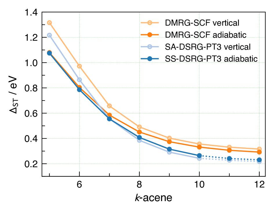
Figure 2: Singlet–triplet gaps of oligoacenes obtained using DMRG-SCF and DSRG-PT3 with the def2-TZVP basis set. The DSRG-PT3 results of undecacene and dodecacene are estimated using the additive assumption $\Delta_{\rm ST}^{\text{PT3/def2-TZVP}}=\Delta_{\rm ST}^{\text{PT3/def2-SVP}}-\Delta_{\rm ST}^{\text{PT2/def2-SVP}}+\Delta_{\rm ST}^{\text{PT2/def2-TZVP}}$.

In Table 3, we list the adiabatic $\Delta_{\rm ST}$ of oligoacenes obtained using numerous theoretical methods. Similar to the findings of vertical $\Delta_{\rm ST}$, the DSRG-PT3 and sq-LDSRG(2) methods yield nearly identical adiabatic $\Delta_{\rm ST}$ and they are higher than the DSRG-PT2 predictions by 0.15 eV on average with the def2-SVP basis set. The DSRG adiabatic $\Delta_{\rm ST}$ is noticeably lower than the vertical counterpart for small acenes ($k<8$). As the acene size grows, the difference between the adiabatic and vertical $\Delta_{\rm ST}$ decreases to less than 0.04 eV (see Fig. 2), indicating that the geometry plays a minor role in the $\Delta_{\rm ST}$ of large oligoacenes. Indeed, previous findings also suggest highly analogous bond-length alternation pattern in singlet and triplet geometries in oligoacenes beyond octacene.Mullinax et al. (2019) However, accurate predictions on adiabatic $\Delta_{\rm ST}$ may still require geometries that go beyond density function theory. The comparison between the ACI- and DMRG-DSRG-PT2 data suggests that the ACI reference may be overly truncated for hexacene and heptacene as the DSRG-PT2 values of the two references differ by more than 0.07 eV. Comparing to other methods, our best estimate of the adiabatic $\Delta_{\rm ST}$ from the DSRG-PT3/def2-TZVP method demonstrates surprising agreement with DMRG-AC0 and CCSD(T) with a mean absolute deviation of 0.03 eV.

IV.2. Vertical excitation energies of zeaxanthin

The SA-DMRG-DSRG vertical transitions of zeaxanthin are presented in Table 4. In general, all SA-DSRG methods support the sequence of $\rm 2\,^{1}A_{g}^{-}<1\,^{1}B_{u}^{+}<1\,^{1}B_{u}^{-}$. Taking the SA-sq-LDSRG(2) data as reference, the predictions of SA-DSRG-PT2 are underestimated by 0.17 eV on average. Increasing the size of basis set from double-$\zeta$ to triple-$\zeta$ significantly reduces the vertical transition energy (VTE) of $\rm 1\,^{1}B_{u}^{+}$ by 0.15 eV and 0.19 eV for SA-DSRG-PT2 and PT3, respectively. The other two states are less sensitive to the basis set, resulting in a decrease in VTE from 0.05 to 0.07 eV. In addition, Table 4 includes the SA-DSRG-PT3/def2-TZVP results derived from the ground-state DMRG-SCF(22,22)/cc-pVDZ geometry. Despite the consistent relative ordering of these states, the SA-DSRG-PT3/def2-TZVP VTEs obtained from different geometries show an average variation of 0.09 eV.

Table 4: Vertical excitation energies ($\omega$, in eV) and oscillator strengths ($f$) of zeaxanthin obtained using various SA-DMRG-DSRG methods.

	def2-SV(P)						def2-TZVP
	PT2		PT3		sq-L2		PT2		PT3		PT3a
state	$\omega$	$f$	$\omega$	$f$	$\omega$	$f$	$\omega$	$f$	$\omega$	$f$	$\omega$	$f$
$\rm 2\,^{1}A_{g}^{-}$	$3.12$	$0.002$	$3.32$	$0.000$	$3.27$	$0.001$	$3.07$	$0.005$	$3.26$	$0.001$	$3.35$	$0.001$
$\rm 1\,^{1}B_{u}^{+}$	$3.39$	$3.720$	$3.75$	$3.309$	$3.59$	$3.699$	$3.24$	$3.775$	$3.56$	$3.686$	$3.65$	$3.565$
$\rm 1\,^{1}B_{u}^{-}$	$3.70$	$0.176$	$3.93$	$0.575$	$3.87$	$0.217$	$3.65$	$0.108$	$3.86$	$0.193$	$3.94$	$0.191$

• The ground-state DMRG-SCF(22,22)/cc-pVDZ geometry.

In Table 5, we compare the VTEs of zeaxanthin obtained from SA-DMRG-DSRG and other theoretical approaches. The effect of dynamical correlation is prominently evident in the optically bright $\rm 1\,^{1}B_{u}^{+}$ state, where the SA-DMRG VTE is lowered by over 1.85 eV as a result of the SA-DSRG treatment of electron correlation. The current predictions of SA-DSRG-PT2 are generally higher than those previously reported using a larger flow parameter,Khokhlov and Belov (2022) particularly for the $\rm 1\,^{1}B_{u}^{+}$ state. However, the benchmark on butadiene reveals a substantial underestimation of the $\rm 1\,^{1}B_{u}^{+}$ state in SA-DSRG-PT2 using a converged flow parameter.Wang, Fang, and Li (2023) As also suggested by the def2-SV(P) results, we speculate that the SA-DSRG-PT3 VTEs of zeaxanthin are generally overestimated. Indeed, the experimental value of the $\rm 1\,^{1}B_{u}^{+}$ state, albeit corresponding to adiabatic excitations, is only 2.48 eV.Josue and Frank (2002)

Table 5: Theoretical estimates for the low-lying vertical excitation energies (in eV) of zeaxanthin.

			SA-DMRG-DSRG
state	DFT/MRCIa	SA-DMRGb	PT2c	PT2b	PT3b
$\rm 2\,^{1}A_{g}^{-}$	$2.11$	$3.59$	$2.92$	$3.07$	$3.26$
$\rm 1\,^{1}B_{u}^{+}$	$2.48$	$5.41$	$2.90$	$3.24$	$3.56$
$\rm 1\,^{1}B_{u}^{-}$	$2.75$	$4.19$		$3.65$	$3.86$

• Ref. 67, B3LYP/6-311G(d) geometry.

• This work, def2-TZVP basis set, CAM-B3LYP/cc-pVDZ geometry.

• Ref. 52, cc-pVDZ basis set, CAM-B3LYP/cc-pVDZ geometry, flow parameter $s=1.0$ $E_{\rm h}^{-2}$.

IV.3. Ground-state potential energy curve of Cr2

Figure 3 depicts the ground-state $X\,^{1}\Sigma_{\rm g}^{+}$ potential energy curve (PEC) of Cr2. The experimental PEC fitLarsson et al. (2022) is shifted so that the bottom of the well meets the experimental dissociation energy of 1.56 eV.Simard et al. (1998) As shown in the left panel of Fig. 3, the shape of the experimental PEC is qualitatively reproduced by DSRG-PT3 and sq-LDSRG(2). However, relative to the dissociation limit, the DSRG energies are significantly underestimated by more than 0.16 eV for bond lengths ($r_{\rm Cr-Cr}$) greater than 1.9 Å. Analogous to previous findings,Kurashige and Yanai (2011); Guo et al. (2016); Vancoillie, Malmqvist, and Veryazov (2016) the use of double-shell active space leads to an improved description of the entire PEC over that of the valence active space. Figure 3 also presents the DSRG-PT3 results without reference relaxation [i.e., Eq. (5) is skipped], labeled as uDSRG-PT3.Li and Evangelista (2017) Comparing to the default DSRG-PT3 that incorporates this effect, the reference relaxation deepens the potential well by 0.10–0.15 eV in the bonding region of 1.5–2.1 Å.

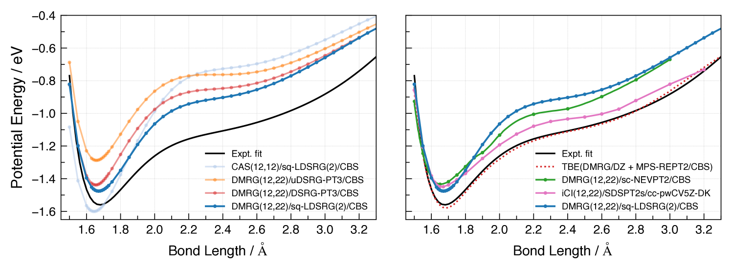
Figure 3: The ground-state potential energy curves of Cr2. The curves of theoretical best estimate (TBE) and experimental fit are taken from Ref. 23.

In the right panel of Fig. 3, we compare the sq-LDSRG(2) PEC to a few selected theoretical methods, including the strongly contracted NEVPT2 (sc-NEVPT2)Guo et al. (2016) and the static-dynamic-static second-order perturbation theory with selection (SDSPT2s) based on an iterative configuration interaction (iCI) reference.Lei et al. (2025) These multireference perturbation theories yield comparable equilibrium bond distance and dissociation energy to those of sq-LDSRG(2). However, the PEC of $r_{\rm Cr-Cr}$ ¿ 1.9 Å is better described by SDSPT2s than sc-NEVPT2 and sq-LDSRG(2). This observation suggests that the coupling between excited configurations inside and outside the active space may be of importance for Cr2.

We report the spectroscopic constants of the ground-state Cr2 in Table 6. The DSRG values were obtained by fitting the PEC using 11 data points near the equilibrium based on the weighted least squares approach.Bender et al. (2014) The DMRG-sq-LDSRG(2)/CBS predictions are in reasonable agreements with the theoretical best estimates (TBE),Larsson et al. (2022) deviated by 0.014 Å, 10 cm^-1, and 0.10 eV for equilibrium bond length ($r_{e}$), harmonic vibrational frequency ($\omega_{e}$), and dissociation energy ($D_{e}$), respectively. We also observe good agreements between DMRG-sq-LDSRG(2)/CBS and the experiment of Ref. 111, differing by 0.01 Å, 26 cm^-1, and 0.01 eV for $r_{e}$, $\omega_{e}$, and $D_{e}$, respectively.

Table 6: Spectroscopic constants (equilibrium bond length $r_{e}$, harmonic vibrational frequency $\omega_{e}$, fundamental vibrational frequency $\Delta G_{1/2}$, dissociation energy with respect to the bottom of the potential $D_{e}$) for the ground-state of Cr2.

method	active space	basis set	$r_{e}$ / Å	$\omega_{e}$ / cm-1	$\Delta G_{1/2}$ / cm-1	$D_{e}$ / eV	reference
sq-LDSRG(2)	(12,12)	CBS(QZ/5Z)	$1.644$	$572$	$556$	$1.60$	this work
DMRG-DSRG-PT3	(12,22)	CBS(QZ/5Z)	$1.655$	$579$	$553$	$1.44$	this work
DMRG-sq-LDSRG(2)	(12,22)	CBS(QZ/5Z)	$1.671$	$505$	$487$	$1.48$	this work
DMRG-CASPT2/$\rm g_{1}$	(12,28)	cc-pwCV5Z	$1.681$	$480$		$1.61$	Ref. 24
RASPT2a	(12,22)	CBS(QZ/5Z)	$1.666$	$489$		$1.89$	Ref. 108
DMRG-sc-NEVPT2	(12,22)	CBS(QZ/5Z)	$1.656$	$470$		$1.43$	Ref. 25
iCI-SDSPT2s	(12,22)	cc-pwCV5Z-DK	$1.659$	$462$		$1.45$	Ref. 109
MRAQCCb	(12,12)	CBS(TZ/QZ)	$1.685$	$459$	$431$	$1.36$	Ref. 73
DMRG-ec-MRCISD+Q	(12,42)	ANO-RCC-VQZP	$1.71$	$477$		$1.62$	Ref. 15
TBE		CBS(QZ/5Z)	$1.685$	$495$	$468$	$1.58$	Ref. 23
experiments			$1.6788$	$470$	$452.34\pm 0.02$		Ref. 112
			$1.68$	$479$		$1.472\pm 0.052$	Ref. 111
				$480.6\pm 0.5$	$455\pm 10$		Ref. 75
						$1.56\pm 0.06$c	Ref. 107

• RASPT2: restricted active space second-order perturbation theory.

• MRAQCC: multireference averaged quadratic coupled cluster.

• A zero-point energy of 0.03 eV is applied to the experimental $D_{0}=1.53\pm 0.06$ value.

V. Conclusions

In this work, we have combined DMRG and SA-DSRG to achieve an accurate description of both static and dynamical electron correlation in strongly correlated molecular systems. A straightforward joint of these two methods can be routinely applied to molecules requiring 30–40 active orbitals at either MRPT or MRCC level of the SA-DSRG theory. Moreover, we have implemented the algorithm of forming the MPS-compressed intermediates,Sokolov et al. (2017) which enables SA-DSRG-PT2 and PT3 computations on dodecacene with an active space of (50,50). To the best of our knowledge, this active space is the largest employed in the internally contracted formalism of multireference theories.

We have performed DMRG-DSRG computations on the singlet-triplet gaps of oligoacenes, the low-lying vertical excitations of zeaxanthin, and the ground-state potential energy curve of chromium dimer. For large oligoacenes, the vertical and adiabatic $\Delta_{\rm ST}$ values are found nearly identical, differing by less than 0.04 eV. Our best estimates of the vertical and adiabatic $\Delta_{\rm ST}$ of dodecacene are 0.22 and 0.23 eV, respectively. For zeaxanthin, we find that all SA-DSRG methods follow the order of $\rm 2\,^{1}A_{g}^{-}<1\,^{1}B_{u}^{+}<1\,^{1}B_{u}^{-}$ on vertical excitation energies. The shape of the Cr2 ground-state potential energy curve is also reasonably reproduced by DMRG(12,22)-sq-LDSRG(2), showing an equilibrium bond length of 1.671 Å and an harmonic frequency of 505 cm^-1.

This work motivates further developments of DMRG-DSRG. Given the previously noted inconsistencies of C-C bond lengths in DFT and v2RDM optimized geometries,Mullinax et al. (2019) it may be useful to develop the analytic energy gradientsWang, Li, and Evangelista (2021); Park (2022) for DMRG-DSRG-PT2 to assess the impact of molecular geometry on the oligoacene series. Additionally, improving the DSRG-PT3 and LDSRG(2) implementations are essential for computations involving large basis sets. Future benchmark studies on transition-metal complexes are also warranted for DMRG-based DSRG-PT3 and LDSRG(2) methods. Nevertheless, we believe that DMRG-DSRG opens up new applications in the realm of conjugated molecules, including nanographenes,Yu and Heine (2023) chlorophylls, and carotenoids.Accomasso et al. (2024)

Author Contributions

C.L.: conceptualization, data curation, formal analysis, funding acquisition, investigation, methodology, resources, software, supervision, visualization, writing – original draft, writing – review & editing. X.W.: data curation, formal analysis, investigation, visualization, writing – review & editing. H.Z.: formal analysis, methodology, software, writing – review & editing. W.F.: funding acquisition, resources, writing – review & editing.

References

- Vogiatzis et al. (2017) K. D. Vogiatzis, D. Ma, J. Olsen, L. Gagliardi, and W. A. de Jong, J. Chem. Phys. 147, 184111 (2017).
- White (1992) S. R. White, Phys. Rev. Lett. 69, 2863 (1992).
- Schollwöck (2011) U. Schollwöck, Ann. Phys. (N. Y). 326, 96 (2011).
- Chan et al. (2016) G. K.-L. Chan, A. Keselman, N. Nakatani, Z. Li, and S. R. White, J. Chem. Phys. 145, 014102 (2016).
- Evangelisti, Daudey, and Malrieu (1983) S. Evangelisti, J.-P. Daudey, and J.-P. Malrieu, Chem. Phys. 75, 91 (1983).
- Schriber and Evangelista (2016) J. B. Schriber and F. A. Evangelista, J. Chem. Phys. 144, 161106 (2016).
- Holmes, Tubman, and Umrigar (2016) A. A. Holmes, N. M. Tubman, and C. J. Umrigar, J. Chem. Theory Comput. 12, 3674 (2016).
- Liu and Hoffmann (2016) W. Liu and M. R. Hoffmann, J. Chem. Theory Comput. 12, 1169 (2016).
- Booth, Thom, and Alavi (2009) G. H. Booth, A. J. W. Thom, and A. Alavi, J. Chem. Phys. 131, 054106 (2009).
- Gidofalvi and Mazziotti (2008) G. Gidofalvi and D. A. Mazziotti, J. Chem. Phys. 129, 134108 (2008).
- Fosso-Tande et al. (2016) J. Fosso-Tande, T.-S. Nguyen, G. Gidofalvi, and A. E. DePrince, J. Chem. Theory Comput. 12, 2260 (2016).
- Sharma et al. (2017a) S. Sharma, A. A. Holmes, G. Jeanmairet, A. Alavi, and C. J. Umrigar, J. Chem. Theory Comput. 13, 1595 (2017a).
- Zhai and Chan (2021) H. Zhai and G. K.-L. Chan, J. Chem. Phys. 154, 224116 (2021), arXiv:2103.09976 .
- Szalay et al. (2012) P. G. Szalay, T. Müller, G. Gidofalvi, H. Lischka, and R. Shepard, Chem. Rev. 112, 108 (2012).
- Luo et al. (2018) Z. Luo, Y. Ma, X. Wang, and H. Ma, J. Chem. Theory Comput. 14, 4747 (2018).
- Andersson, Malmqvist, and Roos (1992) K. Andersson, P.-Å. Malmqvist, and B. O. Roos, J. Chem. Phys. 96, 1218 (1992).
- Angeli et al. (2001) C. Angeli, R. Cimiraglia, S. Evangelisti, T. Leininger, and J.-P. Malrieu, J. Chem. Phys. 114, 10252 (2001).
- Sharma et al. (2017b) S. Sharma, G. Knizia, S. Guo, and A. Alavi, J. Chem. Theory Comput. 13, 488 (2017b).
- Lyakh et al. (2012) D. I. Lyakh, M. Musiał, V. F. Lotrich, and R. J. Bartlett, Chem. Rev. 112, 182 (2012).
- Evangelista (2018) F. A. Evangelista, J. Chem. Phys. 149, 030901 (2018).
- Sokolov et al. (2017) A. Y. Sokolov, S. Guo, E. Ronca, and G. K.-L. Chan, J. Chem. Phys. 146, 244102 (2017).
- Andersson et al. (1994) K. Andersson, B. Roos, P.-Å. Malmqvist, and P.-O. Widmark, Chem. Phys. Lett. 230, 391 (1994).
- Larsson et al. (2022) H. R. Larsson, H. Zhai, C. J. Umrigar, and G. K.-L. Chan, J. Am. Chem. Soc. 144, 15932 (2022), arXiv:2206.10738 .
- Kurashige and Yanai (2011) Y. Kurashige and T. Yanai, J. Chem. Phys. 135, 094104 (2011).
- Guo et al. (2016) S. Guo, M. A. Watson, W. Hu, Q. Sun, and G. K.-L. Chan, J. Chem. Theory Comput. 12, 1583 (2016).
- Kurashige et al. (2014) Y. Kurashige, J. Chalupský, T. N. Lan, and T. Yanai, J. Chem. Phys. 141, 174111 (2014).
- Phung, Wouters, and Pierloot (2016) Q. M. Phung, S. Wouters, and K. Pierloot, J. Chem. Theory Comput. 12, 4352 (2016).
- Li Manni et al. (2014) G. Li Manni, R. K. Carlson, S. Luo, D. Ma, J. Olsen, D. G. Truhlar, and L. Gagliardi, J. Chem. Theory Comput. 10, 3669 (2014).
- Pernal (2018) K. Pernal, Phys. Rev. Lett. 120, 013001 (2018).
- Pastorczak and Pernal (2018) E. Pastorczak and K. Pernal, J. Chem. Theory Comput. 14, 3493 (2018).
- Ghosh et al. (2017) S. Ghosh, C. J. Cramer, D. G. Truhlar, and L. Gagliardi, Chem. Sci. 8, 2741 (2017).
- Zuzak et al. (2024) R. Zuzak, M. Kumar, O. Stoica, D. Soler‐Polo, J. Brabec, K. Pernal, L. Veis, R. Blieck, A. M. Echavarren, P. Jelinek, and S. Godlewski, Angew. Chemie Int. Ed. 63, e202317091 (2024).
- Evangelista (2014) F. A. Evangelista, J. Chem. Phys. 141, 054109 (2014).
- Li and Evangelista (2019) C. Li and F. A. Evangelista, Annu. Rev. Phys. Chem. 70, 245 (2019).
- Hergert et al. (2014) H. Hergert, S. K. Bogner, T. D. Morris, S. Binder, A. Calci, J. Langhammer, and R. Roth, Phys. Rev. C 90, 041302 (2014).
- Yanai and Chan (2006) T. Yanai and G. K.-L. Chan, J. Chem. Phys. 124, 194106 (2006).
- Yanai and Chan (2007) T. Yanai and G. K.-L. Chan, J. Chem. Phys. 127, 104107 (2007).
- Datta, Kong, and Nooijen (2011) D. Datta, L. Kong, and M. Nooijen, J. Chem. Phys. 134, 214116 (2011).
- Hanauer and Köhn (2011) M. Hanauer and A. Köhn, J. Chem. Phys. 134, 204111 (2011).
- Li and Evangelista (2016) C. Li and F. A. Evangelista, J. Chem. Phys. 144, 164114 (2016).
- Li and Evangelista (2015) C. Li and F. A. Evangelista, J. Chem. Theory Comput. 11, 2097 (2015).
- Li and Evangelista (2017) C. Li and F. A. Evangelista, J. Chem. Phys. 146, 124132 (2017).
- Li and Evangelista (2018) C. Li and F. A. Evangelista, J. Chem. Phys. 148, 124106 (2018).
- Zhang, Li, and Evangelista (2019) T. Zhang, C. Li, and F. A. Evangelista, J. Chem. Theory Comput. 15, 4399 (2019).
- Li and Evangelista (2021) C. Li and F. A. Evangelista, J. Chem. Phys. 155, 114111 (2021), arXiv:2106.07097 .
- Phung, Nam, and Saitow (2023) Q. M. Phung, H. N. Nam, and M. Saitow, J. Phys. Chem. A 127, 7544 (2023).
- Wang, Fang, and Li (2023) M. Wang, W.-H. Fang, and C. Li, J. Chem. Theory Comput. 19, 122 (2023).
- Huang and Evangelista (2023) M. Huang and F. A. Evangelista, J. Chem. Phys. 158, 124112 (2023), arXiv:2212.04369 .
- Huang and Evangelista (2024) M. Huang and F. A. Evangelista, J. Chem. Theory Comput. 20, 7990 (2024).
- Schriber et al. (2018) J. B. Schriber, K. P. Hannon, C. Li, and F. A. Evangelista, J. Chem. Theory Comput. 14, 6295 (2018).
- Khokhlov and Belov (2021) D. Khokhlov and A. Belov, J. Chem. Theory Comput. 17, 4301 (2021).
- Khokhlov and Belov (2022) D. Khokhlov and A. Belov, J. Phys. Chem. A 126, 4376 (2022).
- Li et al. (2017) C. Li, P. Verma, K. P. Hannon, and F. A. Evangelista, J. Chem. Phys. 147, 074107 (2017).
- Tönshoff and Bettinger (2021) C. Tönshoff and H. F. Bettinger, Chem. – A Eur. J. 27, 3193 (2021).
- Hachmann et al. (2007) J. Hachmann, J. J. Dorando, M. Avilés, and G. K.-L. Chan, J. Chem. Phys. 127, 134309 (2007).
- Yang, Davidson, and Yang (2016) Y. Yang, E. R. Davidson, and W. Yang, Proc. Natl. Acad. Sci. 113, E5098 (2016).
- Trinquier, David, and Malrieu (2018) G. Trinquier, G. David, and J.-P. Malrieu, J. Phys. Chem. A 122, 6926 (2018).
- Mondal, Shah, and Neckers (2006) R. Mondal, B. K. Shah, and D. C. Neckers, J. Am. Chem. Soc. 128, 9612 (2006).
- Shen et al. (2018) B. Shen, J. Tatchen, E. Sanchez‐Garcia, and H. F. Bettinger, Angew. Chemie Int. Ed. 57, 10506 (2018).
- Zuzak et al. (2018) R. Zuzak, R. Dorel, M. Kolmer, M. Szymonski, S. Godlewski, and A. M. Echavarren, Angew. Chemie Int. Ed. 57, 10500 (2018).
- Eisenhut et al. (2020) F. Eisenhut, T. Kühne, F. García, S. Fernández, E. Guitián, D. Pérez, G. Trinquier, G. Cuniberti, C. Joachim, D. Peña, and F. Moresco, ACS Nano 14, 1011 (2020).
- Ruan et al. (2025) Z. Ruan, J. Schramm, J. B. Bauer, T. Naumann, L. V. Müller, F. Sättele, H. F. Bettinger, R. Tonner-Zech, and J. M. Gottfried, J. Am. Chem. Soc. , DOI: 10.1021/jacs.4c13296 (2025).
- Tavan and Schulten (1987) P. Tavan and K. Schulten, Phys. Rev. B 36, 4337 (1987).
- Kopczynski et al. (2007) M. Kopczynski, F. Ehlers, T. Lenzer, and K. Oum, J. Phys. Chem. A 111, 5370 (2007).
- Ostroumov et al. (2013) E. E. Ostroumov, R. M. Mulvaney, R. J. Cogdell, and G. D. Scholes, Science (80-. ). 340, 52 (2013).
- Wang et al. (2005) P. Wang, R. Nakamura, Y. Kanematsu, Y. Koyama, H. Nagae, T. Nishio, H. Hashimoto, and J.-P. Zhang, Chem. Phys. Lett. 410, 108 (2005).
- Andreussi et al. (2015) O. Andreussi, S. Knecht, C. M. Marian, J. Kongsted, and B. Mennucci, J. Chem. Theory Comput. 11, 655 (2015).
- Khokhlov and Belov (2020) D. Khokhlov and A. Belov, J. Phys. Chem. A 124, 5790 (2020).
- Götze and Thiel (2013) J. P. Götze and W. Thiel, Chem. Phys. 415, 247 (2013).
- Scuseria and Schaefer (1990) G. E. Scuseria and H. F. Schaefer, Chem. Phys. Lett. 174, 501 (1990).
- Roos and Andersson (1995) B. O. Roos and K. Andersson, Chem. Phys. Lett. 245, 215 (1995).
- Angeli et al. (2006) C. Angeli, B. Bories, A. Cavallini, and R. Cimiraglia, J. Chem. Phys. 124, 054108 (2006).
- Müller (2009) T. Müller, J. Phys. Chem. A 113, 12729 (2009).
- Li et al. (2020) J. Li, Y. Yao, A. A. Holmes, M. Otten, Q. Sun, S. Sharma, and C. J. Umrigar, Phys. Rev. Res. 2, 012015 (2020), arXiv:1909.12319 .
- Casey and Leopold (1993) S. M. Casey and D. G. Leopold, J. Phys. Chem. 97, 816 (1993).
- White (1993) S. R. White, Phys. Rev. B 48, 10345 (1993).
- Dorando, Hachmann, and Chan (2007) J. J. Dorando, J. Hachmann, and G. K.-L. Chan, J. Chem. Phys. 127, 084109 (2007), arXiv:0707.3121 .
- Sharma and Chan (2012) S. Sharma and G. K.-L. Chan, J. Chem. Phys. 136, 124121 (2012), arXiv:1408.5039 .
- Wouters et al. (2014) S. Wouters, W. Poelmans, P. W. Ayers, and D. Van Neck, Comput. Phys. Commun. 185, 1501 (2014).
- Keller and Reiher (2016) S. Keller and M. Reiher, J. Chem. Phys. 144, 134101 (2016), arXiv:1602.01145 .
- Zhai et al. (2023) H. Zhai, H. R. Larsson, S. Lee, Z.-H. Cui, T. Zhu, C. Sun, L. Peng, R. Peng, K. Liao, J. Tölle, J. Yang, S. Li, and G. K.-L. Chan, J. Chem. Phys. 159, 234801 (2023).
- Zgid et al. (2009) D. Zgid, D. Ghosh, E. Neuscamman, and G. K.-L. Chan, J. Chem. Phys. 130, 194107 (2009).
- Li, Misiewicz, and Evangelista (2023) S. Li, J. P. Misiewicz, and F. A. Evangelista, J. Chem. Phys. 159, 114106 (2023).
- Chatterjee and Sokolov (2020) K. Chatterjee and A. Y. Sokolov, J. Chem. Theory Comput. 16, 6343 (2020).
- Kollmar et al. (2021) C. Kollmar, K. Sivalingam, Y. Guo, and F. Neese, J. Chem. Phys. 155, 234104 (2021).
- Evangelista et al. (2024) F. A. Evangelista, C. Li, P. Verma, K. P. Hannon, J. B. Schriber, T. Zhang, C. Cai, S. Wang, N. He, N. H. Stair, M. Huang, R. Huang, J. P. Misiewicz, S. Li, K. Marin, Z. Zhao, and L. A. Burns, J. Chem. Phys. 161, 062502 (2024).
- MyF (2025) See https://github.com/lcyyork/forte/tree/dmrg_init_orbs, last accessed: Feb. 17 (2025).
- Sharma et al. (2019) P. Sharma, V. Bernales, S. Knecht, D. G. Truhlar, and L. Gagliardi, Chem. Sci. 10, 1716 (2019), arXiv:1808.06273 .
- Pipek and Mezey (1989) J. Pipek and P. G. Mezey, J. Chem. Phys. 90, 4916 (1989).
- Olivares-Amaya et al. (2015) R. Olivares-Amaya, W. Hu, N. Nakatani, S. Sharma, J. Yang, and G. K.-L. Chan, J. Chem. Phys. 142, 034102 (2015).
- Kurashige and Yanai (2009) Y. Kurashige and T. Yanai, J. Chem. Phys. 130, 234114 (2009).
- Hess (1986) B. A. Hess, Phys. Rev. A 33, 3742 (1986).
- Wolf, Reiher, and Hess (2002) A. Wolf, M. Reiher, and B. A. Hess, J. Chem. Phys. 117, 9215 (2002).
- Feller (1993) D. Feller, J. Chem. Phys. 98, 7059 (1993).
- Helgaker et al. (1997) T. Helgaker, W. Klopper, H. Koch, and J. Noga, J. Chem. Phys. 106, 9639 (1997).
- Balabanov and Peterson (2005) N. B. Balabanov and K. A. Peterson, J. Chem. Phys. 123, 064107 (2005).
- Smith et al. (2020) D. G. A. Smith, L. A. Burns, A. C. Simmonett, R. M. Parrish, M. C. Schieber, R. Galvelis, P. Kraus, H. Kruse, R. Di Remigio, A. Alenaizan, A. M. James, S. Lehtola, J. P. Misiewicz, M. Scheurer, R. A. Shaw, J. B. Schriber, Y. Xie, Z. L. Glick, D. A. Sirianni, J. S. O’Brien, J. M. Waldrop, A. Kumar, E. G. Hohenstein, B. P. Pritchard, B. R. Brooks, H. F. Schaefer, A. Y. Sokolov, K. Patkowski, A. E. DePrince, U. Bozkaya, R. A. King, F. A. Evangelista, J. M. Turney, T. D. Crawford, and C. D. Sherrill, J. Chem. Phys. 152, 184108 (2020).
- Pritchard et al. (2019) B. P. Pritchard, D. Altarawy, B. Didier, T. D. Gibson, and T. L. Windus, J. Chem. Inf. Model. 59, 4814 (2019).
- Stoychev, Auer, and Neese (2017) G. L. Stoychev, A. A. Auer, and F. Neese, J. Chem. Theory Comput. 13, 554 (2017).
- Li et al. (2024) C. Li, S. Mao, R. Huang, and F. A. Evangelista, J. Chem. Theory Comput. 20, 4170 (2024).
- Beran et al. (2021) P. Beran, M. Matoušek, M. Hapka, K. Pernal, and L. Veis, J. Chem. Theory Comput. 17, 7575 (2021), arXiv:2108.12803 .
- Hajgató, Huzak, and Deleuze (2011) B. Hajgató, M. Huzak, and M. S. Deleuze, J. Phys. Chem. A 115, 9282 (2011).
- East and Allen (1993) A. L. L. East and W. D. Allen, J. Chem. Phys. 99, 4638 (1993).
- Véril et al. (2021) M. Véril, A. Scemama, M. Caffarel, F. Lipparini, M. Boggio‐Pasqua, D. Jacquemin, and P. Loos, WIREs Comput. Mol. Sci. 11, e1517 (2021), arXiv:2011.14675 .
- Mullinax et al. (2019) J. W. Mullinax, E. Epifanovsky, G. Gidofalvi, and A. E. DePrince, J. Chem. Theory Comput. 15, 276 (2019).
- Josue and Frank (2002) J. S. Josue and H. A. Frank, J. Phys. Chem. A 106, 4815 (2002).
- Simard et al. (1998) B. Simard, M.-A. Lebeault-Dorget, A. Marijnissen, and J. J. ter Meulen, J. Chem. Phys. 108, 9668 (1998).
- Vancoillie, Malmqvist, and Veryazov (2016) S. Vancoillie, P. Å. Malmqvist, and V. Veryazov, J. Chem. Theory Comput. 12, 1647 (2016).
- Lei et al. (2025) Y. Lei, Y. Guo, B. Suo, and W. Liu, J. Chem. Theory Comput. , DOI: 10.1021/acs.jctc.4c01596 (2025).
- Bender et al. (2014) J. D. Bender, S. Doraiswamy, D. G. Truhlar, and G. V. Candler, J. Chem. Phys. 140, 54302 (2014).
- Hilpert and Ruthardt (1987) K. Hilpert and R. Ruthardt, Berichte der Bunsengesellschaft für Phys. Chemie 91, 724 (1987).
- Bondybey and English (1983) V. Bondybey and J. English, Chem. Phys. Lett. 94, 443 (1983).
- Wang, Li, and Evangelista (2021) S. Wang, C. Li, and F. A. Evangelista, J. Chem. Theory Comput. 17, 7666 (2021), arXiv:2109.14548 .
- Park (2022) J. W. Park, J. Chem. Theory Comput. 18, 2233 (2022), arXiv:2111.07253 .
- Yu and Heine (2023) H. Yu and T. Heine, J. Am. Chem. Soc. 145, 19303 (2023).
- Accomasso et al. (2024) D. Accomasso, G. Londi, L. Cupellini, and B. Mennucci, Nat. Commun. 15, 847 (2024).