ACTIVA: Amortized Causal Effect Estimation without Graphs via
Transformer-based
Variational Autoencoder
Abstract
Predicting the distribution of outcomes under hypothetical interventions is crucial in domains like healthcare, economics, and policy-making. Current methods often rely on strong assumptions, such as known causal graphs or parametric models, and lack amortization across problem instances, limiting their practicality. We propose a novel transformer-based conditional variational autoencoder architecture, named ACTIVA, that extends causal transformer encoders to predict causal effects as mixtures of Gaussians. Our method requires no causal graph and predicts interventional distributions given only observational data and a queried intervention. By amortizing over many simulated instances, it enables zero-shot generalization to novel datasets without retraining. Experiments demonstrate accurate predictions for synthetic and semi-synthetic data, showcasing the effectiveness of our graph-free, amortized causal inference approach.
1 Introduction
Causal effect estimation from observational data is an important task in many domains including healthcare (Shi & Norgeot, 2022), economics (Panizza & Presbitero, 2014), and finance (Kumar et al., 2023). The task can be summarized by the following question: Given observations of certain variables, how will their distribution change when a specific action is performed?
Additionally to answering cause-effect questions, this distribution can provide further task-relevant insights such as uncertainty while preventing erroneous average effect predictions (Rissanen & Marttinen, 2021). However, distributional causal effect estimation is a challenging task, due to possible lack of interventional data, abundance of possibilities for modeling estimated distributions, and the inherent challenges of identifiability from observational data (Bareinboim et al., 2022), among others.
To cope with these difficulties, current approaches often rely on strong assumptions, such as having prior knowledge of the causal graph and imposing parametric assumptions on the underlying causal model (see Section 5 for more detail). For related causal tasks, there have been various proposals to tackle these challenges by extracting causal information from datasets via neural networks (Lorch et al., 2022; Scetbon et al., 2024; Sauter et al., 2024b; Annadani et al., 2025; Hollmann et al., 2025). Results from these approaches suggest that we can effectively amortize over datasets coming from different causal models for various downstream tasks. In a similar setup, amortized causal effect estimation has been studied but with restrictions to scenarios with known causal graphs (Mahajan et al., 2024).
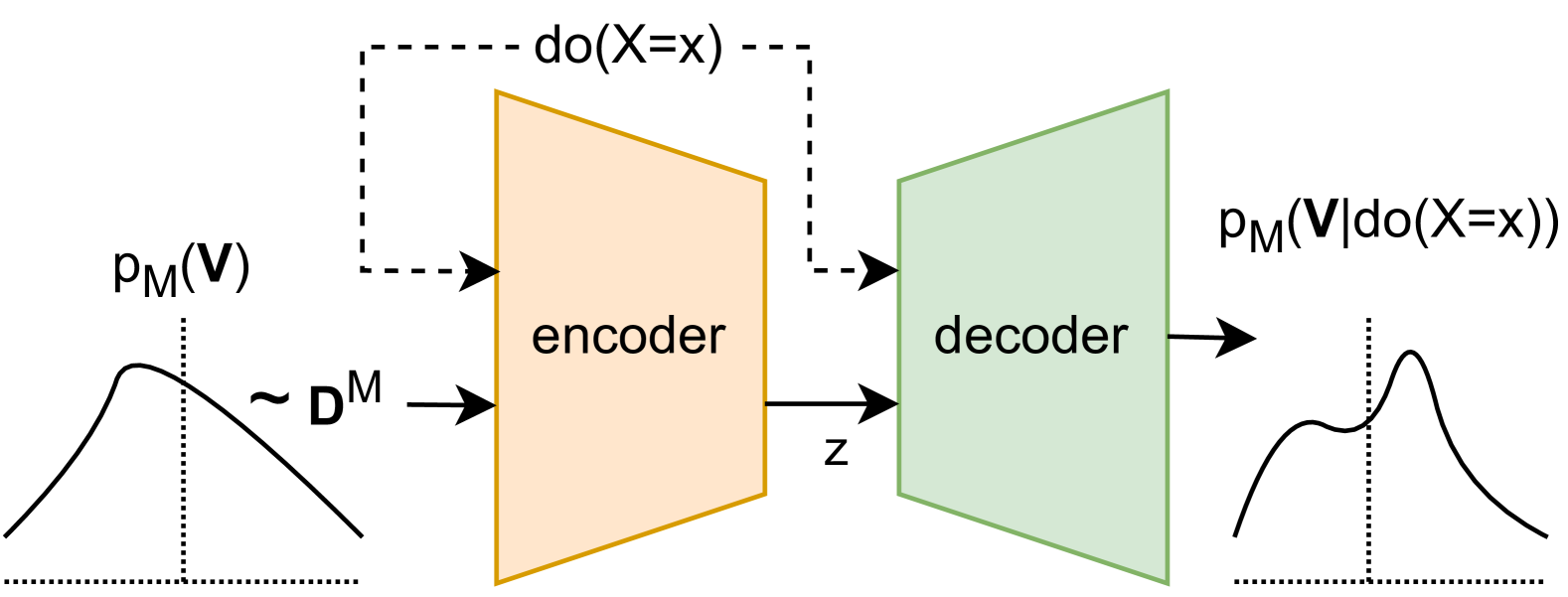
In this paper, we overcome these restrictions by proposing a causal encoder-decoder architecture called ACTIVA. Conditioned on an interventional query, the encoder maps the observational data to a latent space and the conditional decoder transforms the encoded causal information into a mixture of Gaussians, representing the interventional distribution. Moreover, both the encoder and decoder are equivariant regarding variable ordering. We derive the evidence lower bound (ELBO) (Kingma & Welling, 2013) for our amortized learning setup with observational and interventional training data, optimizing for reconstruction of the intervened data while simultaneously regularizing the latent space.
Importantly, there is no need to have access to the underlying causal graph neither during training nor inference, avoiding common pitfalls when relying on such graphs (Poinsot et al., 2024). In empirical evaluations, we show that our architecture can be trained on synthetic data and then be applied to novel instances during inference. This allows for the potential zero-shot transfer from simulated scenarios to the real-world ones. Below we provide a list of our main contributions:
-
•
We provide a conditional encoder-decoder architecture for amortized causal effect prediction. Our model takes an observational dataset and a query intervention as input, predicts a latent representation of the dataset and outputs an estimate of the respective interventional distribution as visualized in Figure 1.
-
•
We formulate a loss function for amortized causal effect prediction based on the ELBO, optimizing for the conditional reconstruction of interventional data from observational data while regularizing the latent space.
-
•
We show empirically that ACTIVA successfully predicts interventional distributions given observational data and interventional queries both on synthetic and semi-synthetic data.
Overall, our work highlights the significance of amortized causal inference as a tool to overcome traditional hurdles in distributional causal effect estimation.111The code to our model is available at https://anonymous.4open.science/r/Amortized_Interventional_Distribution_Estimation-30B2/.
2 Background
2.1 Background on Conditional -VAEs
Variational Autoencoders (VAEs) are generative models that approximate the joint distribution , where are latent variables capturing unobserved variables governing the data. The marginal likelihood is optimized using the ELBO (Kingma & Welling, 2013):
| (1) |
The ELBO balances two terms: the reconstruction term, which ensures the model accurately reconstructs the data from the latent representation, and the Kullback-Leibler (KL) divergence, which regularizes the learned latent distribution to remain close to some pre-defined prior .
Conditional VAEs (CVAEs) (Sohn et al., 2015) extend this framework to conditional distributions , where represents auxiliary information. In -VAEs (Higgins et al., 2017), the KL divergence term is scaled by a hyperparameter , leading to a modified ELBO as follows:
| (2) |
The choice of governs the trade-off between disentangling latent representations and reconstruction fidelity. While emphasizes disentanglement, in our setting, we use to prioritize accurate reconstruction over latent disentanglement.
To enhance flexibility, and reduce over-regularization we adopt the variational mixture of posteriors (VAMP) prior (Tomczak & Welling, 2018), which models the prior through a learnable mixture of variational posteriors:
| (3) |
where are learned parameters that can be thought of as hyperparameters of the prior replacing actual inputs to the encoder.
2.2 Causal Models
In this paper, we employ the notation of structural causal models (SCM) for describing causal data generating processes. For a detailed definition, we refer the reader to (Bareinboim et al., 2022). Specifically, we treat a causal model as a generative process over variables . The model is causal in the sense that each variable is the direct cause of a subset of . Specifically, any variable is determined by its direct causes with , where is an arbitrary function of the direct causes (representing parent variables of ) and a noise term . All causal relations combined form the causal graph . Each model induces a joint distribution , called the observational distribution.
In a causal model, performing a so-called intervention , manipulates such that the target variable is forced to take on value , regardless of ’s causes. Such an intervention results in an intervened model that we denote or when is clear from the context. Analogously, we denote the variables of as . In this work, is one possible intervention value for which the training data contains samples. Similarly to its observational counterpart, induces a joint distribution that we call the interventional distribution.
The task of distributional causal effect estimation is to identify from an observational dataset , where is the number of samples and . In general, estimating this effect is not possible without additional assumptions or interventional data (Bareinboim et al., 2022). This work aims at alleviating this challenge by using interventional data at training time and exploiting the learned, amortized information at inference time without needing interventional data or causal graphs.
3 Model Architecture
We propose a method for amortized prediction of interventional distributions from observational data using a conditional -VAE with VAMP prior. Our model employs a transformer-based encoder (Kossen et al., 2021; Lorch et al., 2022) and decoder that predicts the parameters of a mixture of Gaussians which represents the interventional distribution. This formulation allows us to model arbitrary interventional distributions that are permutation equivariant regarding the variables, i.e. permuting the variable ordering in the input data leads to an equivalent permutation of the dimension of the estimated distribution. Figure 2 gives an overview of our model. More details and hyperparameters can be found in Appendix C.
3.1 Representing Interventions
To effectively condition our VAE on a given intervention, we create a matrix representation of the interventions. More precisely, we consider the index of a possible intervention value , where is the number of possible values, and a selector indicating the target(s) of the intervention. By not encoding the intervention value directly, but rather the index of the intervention, we remove the need to have a full specification of the intervention. This allows us to model interventional distributions based on placeholder IDs of the interventions, as long as they can be attributed to interventional training data.
From and we construct the intervention representation representing as follows. We perform a one-hot encoding of creating a vector and repeat it times, resulting in a matrix . We then apply as a mask to this matrix, effectively zeroing out the rows that correspond to non-intervened variables.
This construction of the conditional of our VAE ensures that the intervention-relevant information for each variable is provided as local information alongside the variable itself. This design guarantees that the information for one variable is stored independently of all other variables, ensuring permutation equivariance of the model with respect to the variable ordering in the data even after conditioning on the intervention.
3.2 Encoder
We model our encoder based on the extension of non-parametric encoders (Kossen et al., 2021) described in (Lorch et al., 2022). As it has been shown for various causal tasks, this encoder architecture can successfully encode a dataset into a vector containing relevant information about the underlying causal model, such as causal structure (Lorch et al., 2022), topological ordering (Scetbon et al., 2024), informative interventions (Annadani et al., 2025), or more abstract prediction tasks (Hollmann et al., 2025). In our setup, we employ this architecture to encode information necessary to predict interventional distributions.
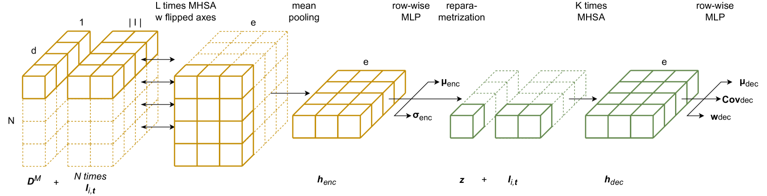
Given a dataset of observational samples from , an intervention index and a binary target vector , the encoder predicts the mean and variance of a multivariate normal Gaussian (MVN) representing the interventional distribution. To do so, we first extend the intervention representation by repeating it times. We then append the expanded representation to the dataset resulting in an augmented dataset . Then we apply blocks of multi-head self-attention (MHSA) that alternate in attending over features and samples. This ensures permutational equivariance to both the sample and the feature dimension (Lorch et al., 2022). Furthermore, we apply layer normalization, residual connections, and dropout following the transformer block setup (Vaswani et al., 2017). After the transformer blocks, we average over the sample axis to obtain an embedding , where indicates the embedding dimension. By taking the average, we ensure that the embedding is permutation invariant regarding the sample dimension. To obtain the mean and log-variance we apply a multi-layer perceptron (MLP) to the embedding of each feature independently. Overall, characterizes a standard normal distribution, where are the parameters of our encoder.
3.3 Decoder
We model the decoder as a transformer with parameters that outputs parameters of a mixture of Gaussians with components, where is an encoding, indicates a possible intervention value , and defines the target vector. This allows us to get a closed-form expression of the estimated interventional distributions.
Similarly to the encoder, we concatenate along the feature dimension of to get the final input to the decoder . After standard transformer blocks (Vaswani et al., 2017), we get the resulting embedding . We feed this embedding through a row-wise linear layer to predict the means , maintaining permutation equivariance regarding the variable ordering. To also predict the covariances in a permutation equivariant manner, we first apply a row-wise linear layer to compute as an intermediate step and then compute the covariances via similarly to (Lorch et al., 2022). To increase numerical stability, we add a small constant to the diagonal of the covariance matrix. Lastly, we predict the component weights of the mixture by first averaging along the feature dimensions and then passing the pooled representation through a linear layer and a softmax layer.
Since encodes causal information as argued in Section 3.2, by conditioning on an intervention via and , we enable our model to estimate interventional distributions. It is noteworthy that we maintain permutation equivariance of the means and covariances of the resulting mixture w.r.t. the ordering of the variables in . This allows us to propagate the permutations of the variables in the input data, through the encoder and the decoder to the estimated interventional distribution.
3.4 Learning Objective
Our model optimizes a conditional version of the ELBO on the log-likelihood of the data. Specifically, we aim to maximize the log-likelihood of the interventional data . We point out that, while SCMs are useful for describing our approach, we do not rely on any specific formalization of causal models to derive our ELBO loss.
To derive our learning objective, we begin by factorizing our conditional distribution in terms of latent variables. Furthermore, as argued in Section 3.2, we assume that the latents together with and contain all information necessary to generate . Hence, we take advantage of the fact that , resulting in the following equality.
| (4) | ||||
| (5) |
We then introduce the conditional variational posterior , parameterized by the output of the encoder and simplify further as shown below222Note that for readability we denote the variational posterior as :
| (6) | ||||
| (7) |
We then apply Jensen’s inequality and rearrange the resulting term into reconstruction and divergence term leading to the ELBO.
| (8) | ||||
| (9) | ||||
where the first term represents the expected log-likelihood of the data given the latent variable and the intervention, and the second term is the KL divergence between the variational posterior and the prior . To make this bound tractable, we approximate the true posterior with the VAMP prior .
We estimate the log-likelihood with samples per interventional distributions in our training set, simultaneously ensuring that the ELBO is maximized for each intervention value and target. To enable gradient-based optimization, we use the reparameterization trick (Kingma & Welling, 2013), allowing backpropagation through the stochastic sampling process of . This results in the reconstruction loss
| (10) |
The second term, the KL divergence , acts as a regularizer, encouraging the variational posterior to remain close to the prior distribution. Similarly to the reconstruction loss, we compute this simultaneously for all intervention-target pairs, resulting in the KL loss
| (11) |
We then define the overall loss of our model as
| (12) |
This formulation is useful to learn a model that predicts the interventional distributions for a single input data set , which needs to be known at training time. To successfully apply our model to data sets that were not in the training data, we expand the objective to an amortizing objective. More specifically, we consider causal models from predefined classes of models. The observational and interventional datasets are sampled from these models, inducing a distribution over these datasets. Optimizing our amortized objective then amounts to minimizing the expectation of our loss regarding the distribution of these datasets:
| (13) |
This objective ensures that our model can make inferences on datasets coming from the class of predefined causal models, even if the specific dataset was not in the training set. It furthermore implies that the more general the training distribution of data sets is, the more the model will generalize to new data sets during inference.
4 Experiments
4.1 Datasets
We evaluate the performance of the proposed method across four different types of datasets: two purely synthetic and one semi-synthetic dataset. Below we provide an overview of each dataset category. For each causal model in these categories, we draw samples from the observational and each interventional distribution. Detailed information on dataset generation and the exact parameters can be found in Appendix A.
Synthetic Data (Gaussian and Beta Noise).
We generate data from linear additive causal models of the form
where is drawn either from a Gaussian distribution or a Beta distribution . We generate data for single-variable interventions on each variable. In general, linear Gaussian-noise models are not identifiable without additional constraints or interventional data, whereas beta-noise models are identifiable from merely observational data (Peters et al., 2017). While it is unclear whether this result transfers to the amortized learning setting in this paper, this aspect makes these two classes of data interesting for comparison.
Semi-Synthetic (SERGIO).
We generate biologically inspired data using the SERGIO simulator (Dibaeinia & Sinha, 2020) for gene-expression. SERGIO models single-cell gene expressions with the resulting data aligning closely with real gene-expression patterns. Notably, we use the implementation provided by (Lorch et al., 2022) that allows interventions in the simulator. We generate data for single-variable interventions on each variable to simulate gene-knockout.
4.2 Metrics
To assess the fidelity of the learned distributions, we rely on three sample-based metrics and a permutation-based statistical test. A detailed introduction to these metrics can be found in Appendix B.
Maximum Mean Discrepancy (MMD).
MMD (Gretton et al., 2012) is a kernel-based measure that compares the mean embeddings of two distributions in a reproducing kernel Hilbert space. Smaller values indicate a closer match in the induced feature space.
Wasserstein Distance (WSD).
WSD (Villani, 2009), captures the minimal “transport cost” required to transform one distribution into another, providing a geometric notion of dissimilarity. Lower values indicate closeness of the samples.
Energy Distance (ERG).
The energy distance (Székely & Rizzo, 2013) indicates pairwise differences between samples from two distributions. A lower energy distance corresponds to higher distributional similarity.
Energy-Based Permutation Test.
We further employ a permutation test using the energy distance to evaluate whether the estimated samples differ significantly from ground-truth data. By comparing the observed energy distance against a null distribution formed via random permutations of the pooled samples, we obtain a statistical measure of distributional mismatch. The higher the resulting p-value, the more our samples are indistinguishable from the samples drawn from the ground-truth distribution.
4.3 Conditional Baseline
We compare with a baseline that estimates the interventional distribution using conditional distributions. Concretely, it fits a multivariate normal (MVN) to the dataset in order to approximate the observational distribution . From the fitted MVN, it derives the conditional distribution . Then, it draws samples from this conditional distribution and assigns the intervention value to each variable in . This approach provides a straightforward conditional baseline, enabling us to compare the degree to which our method captures genuinely causal information, rather than relying solely on conditioning.
4.4 Demonstration of Capturing the Underlying Causal Model
In this experiment, we examine whether our model’s inference procedure indeed captures the causal model of the data-generating process. Specifically, we train our model on the Beta and Gaussian datasets, both described in Section 4.1. We first consider the bivariate case where each dataset consists of pairs of variables under distinct causal mechanisms. Next, we extend this evaluation by training ACTIVA on Gaussian and Beta datasets with 8 variables to show its ability to scale to more complex scenarios. In particular, we train two more models for each of the two datasets. One with a single component (Gaussian1 and Beta1) and one with a mixture of 10 components, (Gaussian10 and Beta10), for the output distribution. This facilitates better comparison to the baseline since it only has one Gaussian for the output distribution as well, while demonstrating the full modeling power of our model. Details about hyperparameter settings are presented in Appendix C.
Quantitative Evaluation.
To assess our method’s performance, we compare it against the conditional baseline on a test set of novel causal models. Table 1 reports the average scores on the two test sets in the bivariate case. Firstly, we observe that ACTIVA outperforms the baseline across all metrics. Secondly, we note that for both datasets, the estimated interventional distributions of our method are not significantly different from the ground-truth interventional distributions on average333Using a 5% significance level., whereas the conditional baseline’s estimates are significantly different. This demonstrates that the distributions that are estimated with ACTIVA are indistinguishable from the ground-truth distribution on average.
| MMD | WSD | ERG | P | ||
|---|---|---|---|---|---|
| Gaussian | baseline | .92 | 6.06 | 11.13 | .00 |
| ACTIVA | .36 | 2.79 | 2.57 | .06 | |
| Beta | baseline | .91 | 6.02 | 11.45 | .00 |
| ACTIVA | .30 | 2.66 | 2.52 | .20 |
Table 2 shows the inference performance on the Gaussian test sets and the conditional baseline for the eight variables case. Results for the Beta models are presented in Section D.1. Even in this more complex task, we observe that ACTIVA outperforms the conditional baseline in terms of MMD and ERG. This becomes even more apparent when we increase the expressiveness of the predicted distribution by adding more components to the Gaussian mixture. In this case, our model’s estimates are almost indistinguishable from the ground truth distribution with an average p-value of . In contrast, the higher WSD reflects a greater “transport cost” in the distribution space, which we attribute to ACTIVA’s tendency to predict higher variances on average.444Average variance of 0.93 for the baseline, 38.8 and 35.91 for Gaussian1 and Gaussian10, respectively.
| mmd | wsd | erg | p | |
|---|---|---|---|---|
| Baseline | .89 | 10.62 | 16.13 | .00 |
| Gaussian 1 | .54 | 13.93 | 11.12 | .001 |
| Gaussian 10 | .49 | 11.83 | 9.31 | .048 |
Qualitative Analysis.
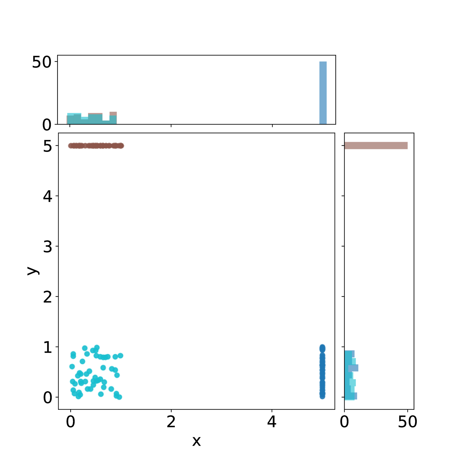
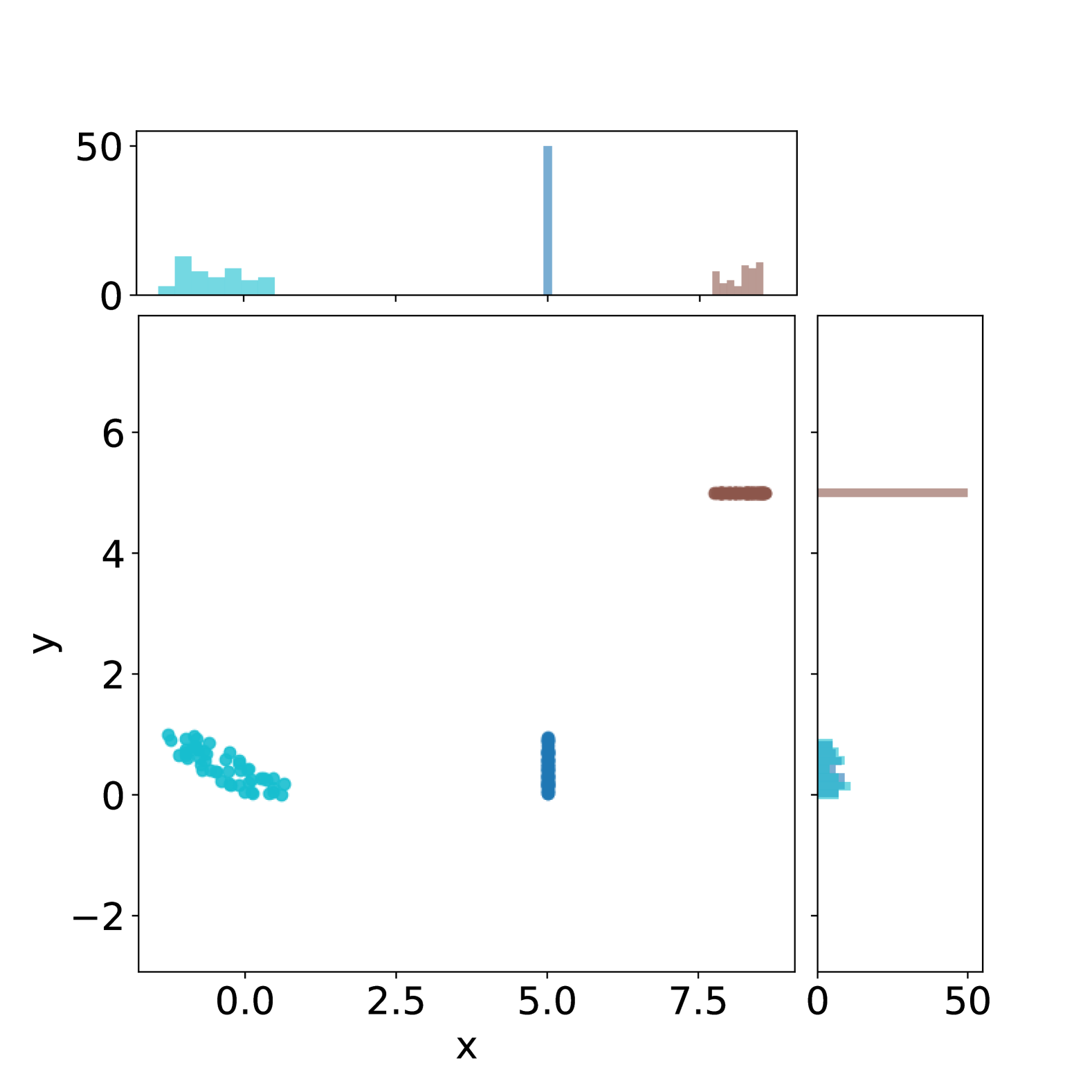
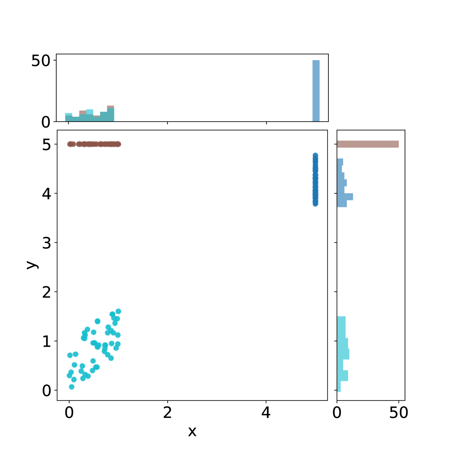
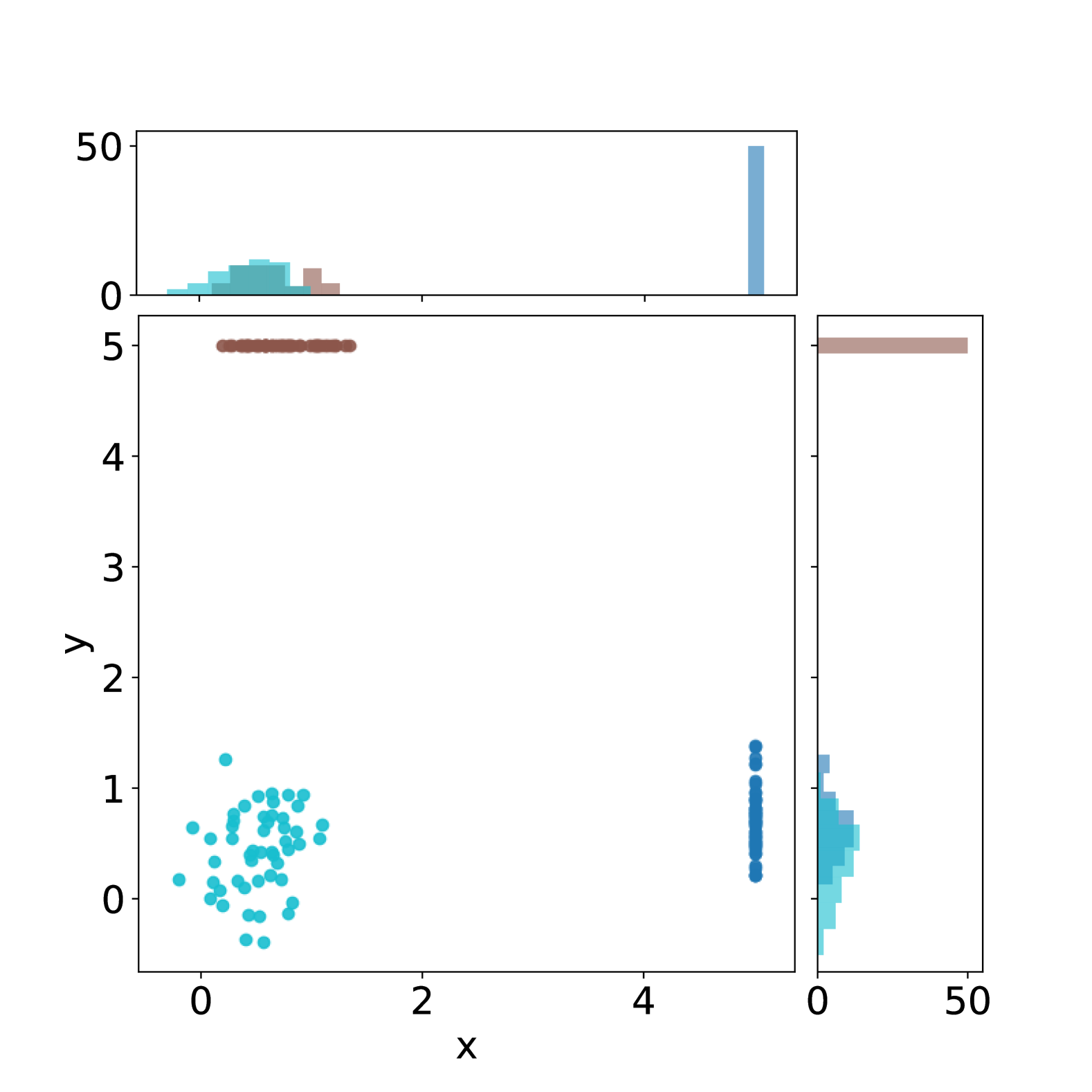
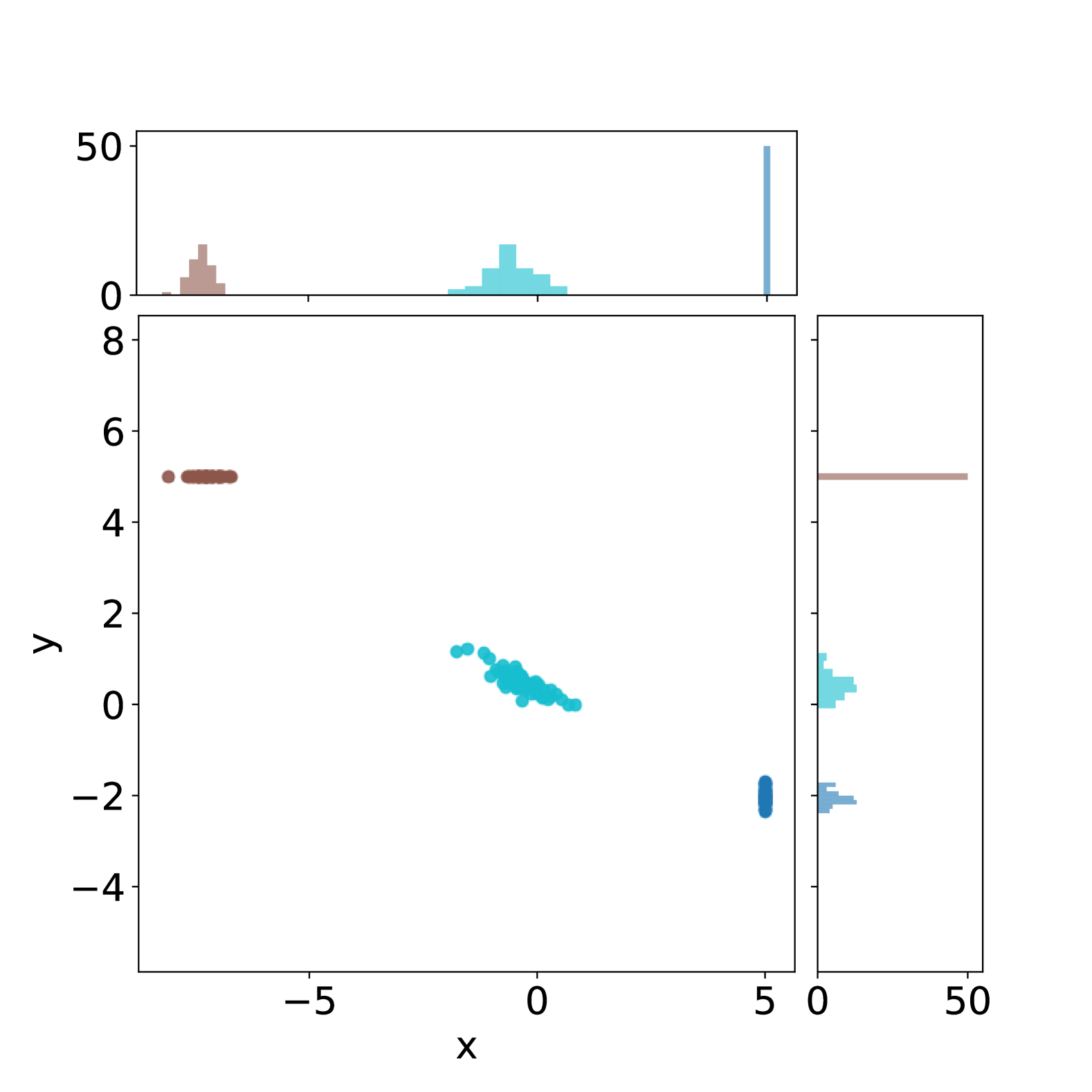
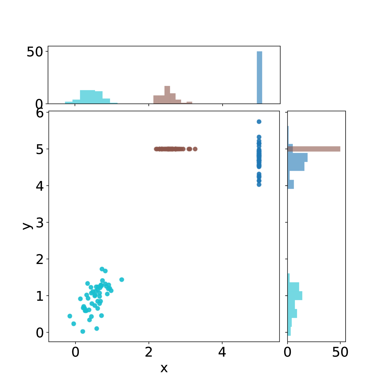
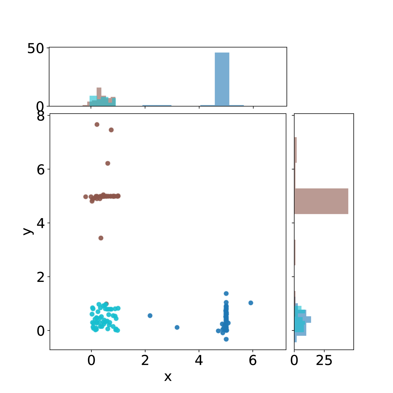
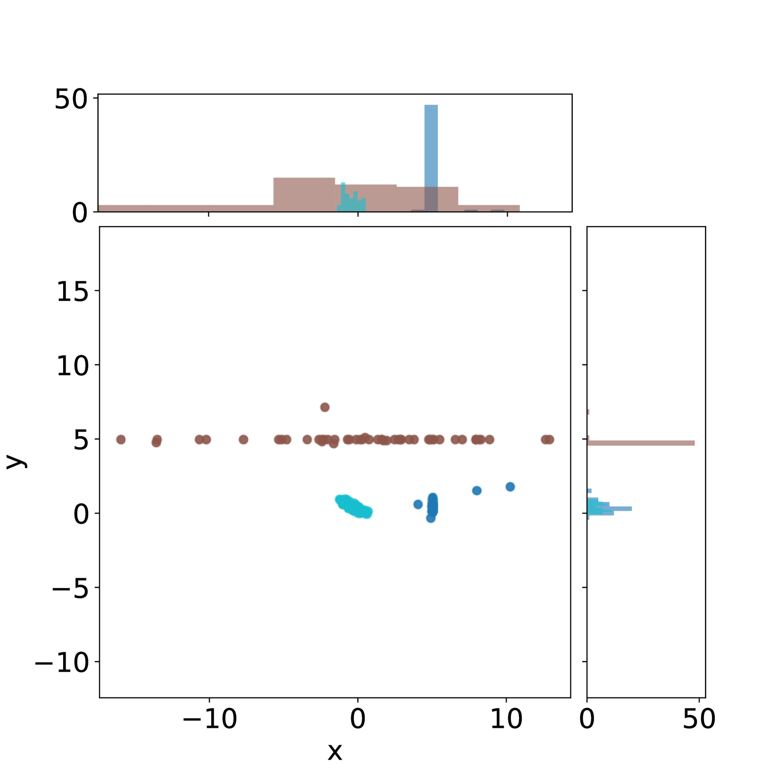
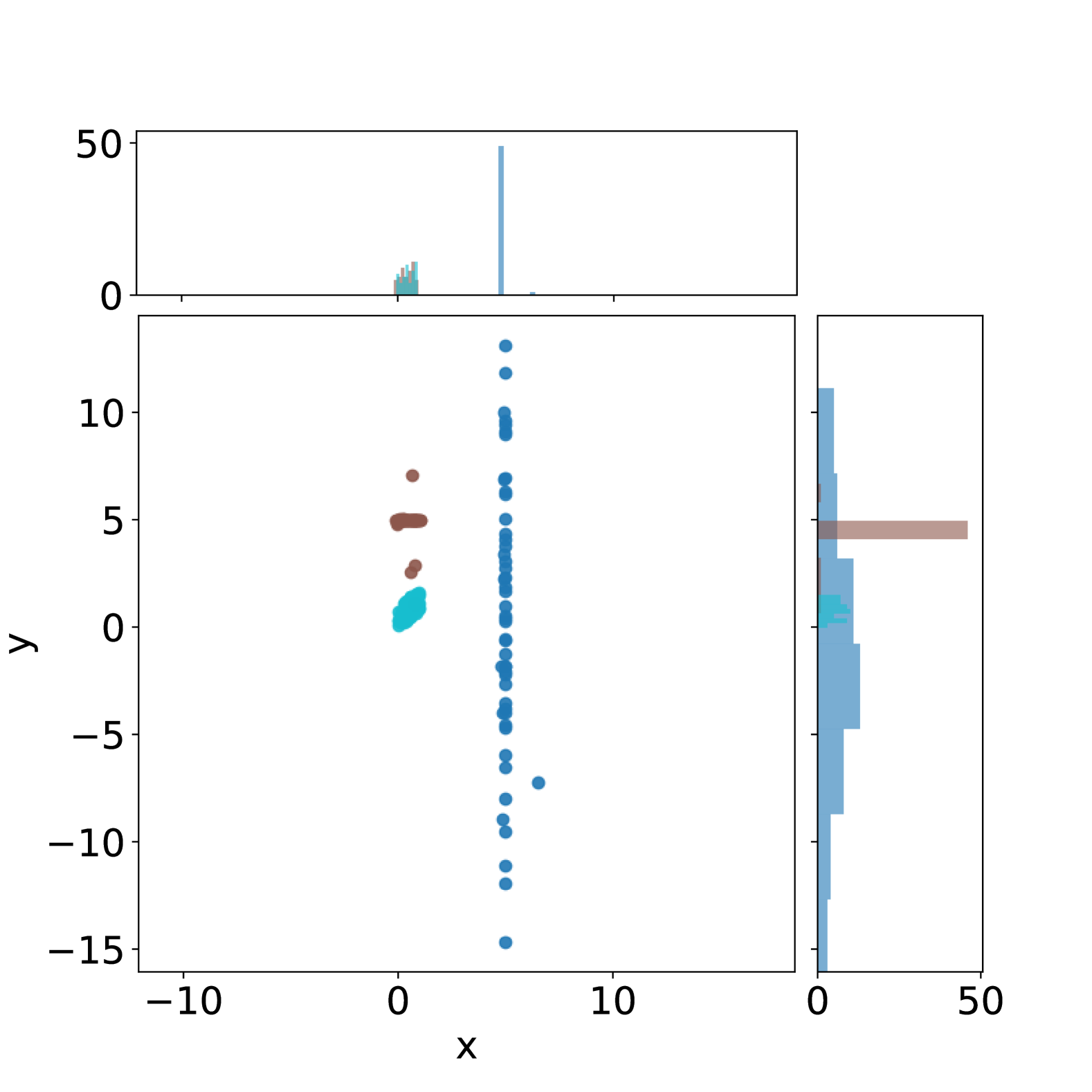
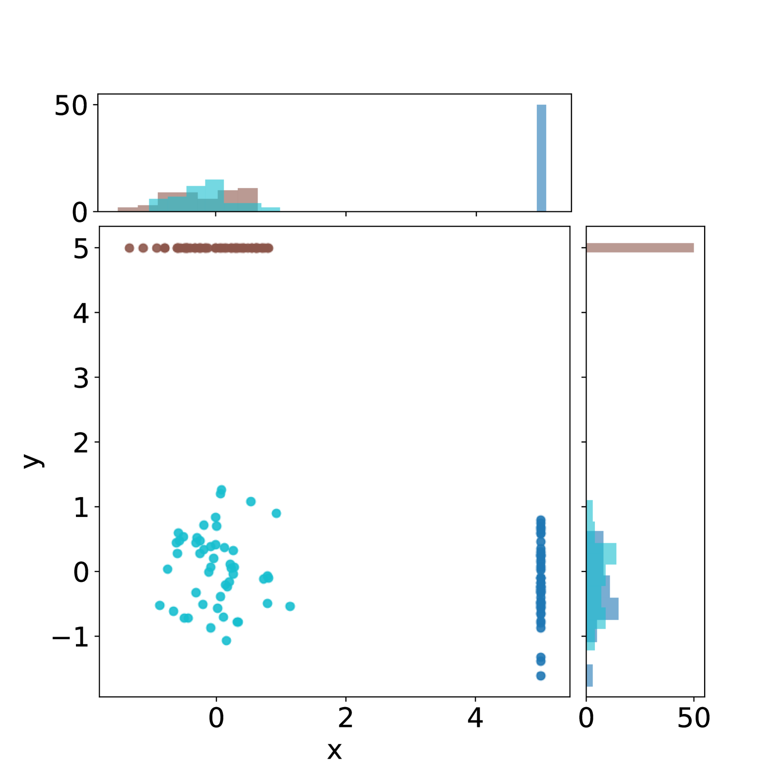
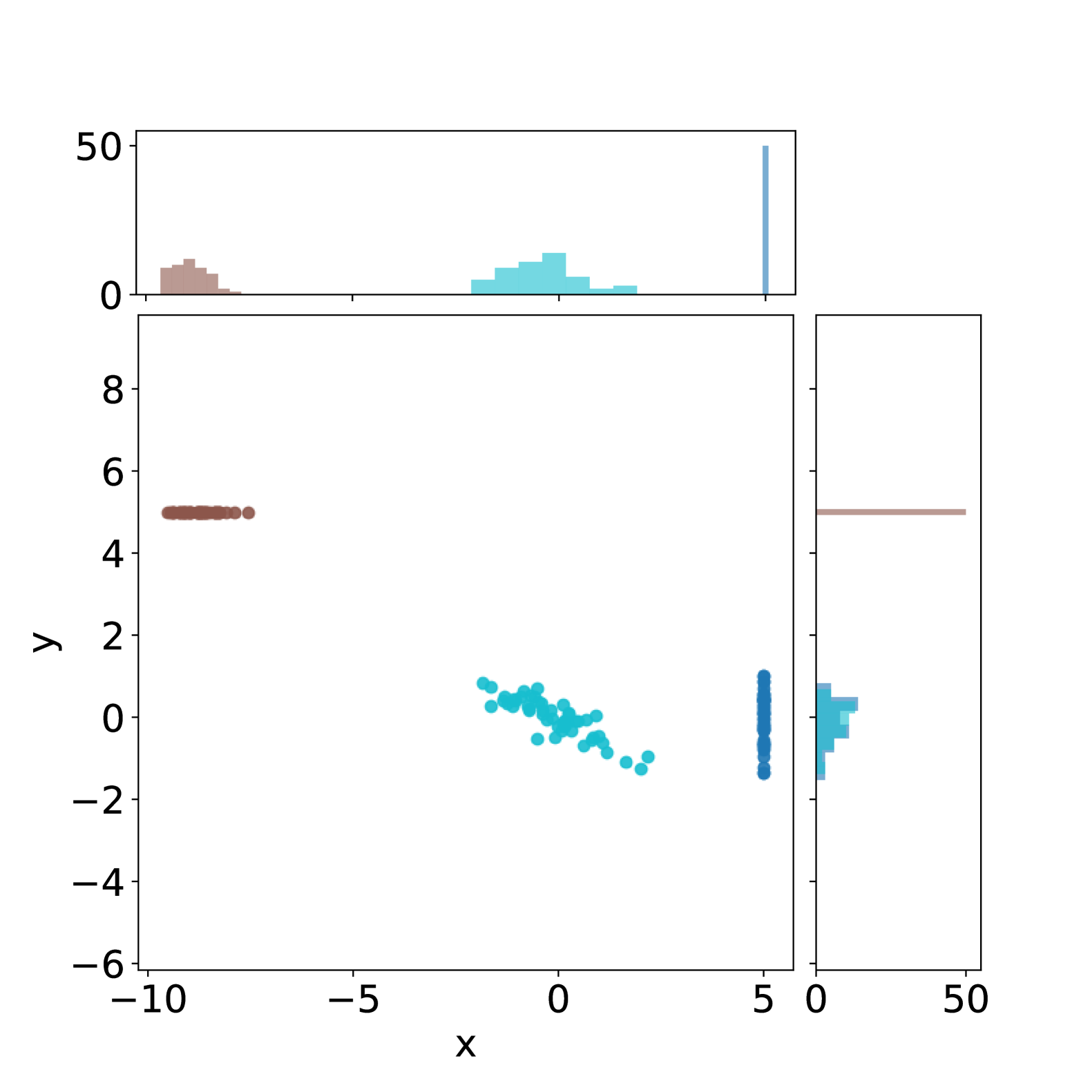
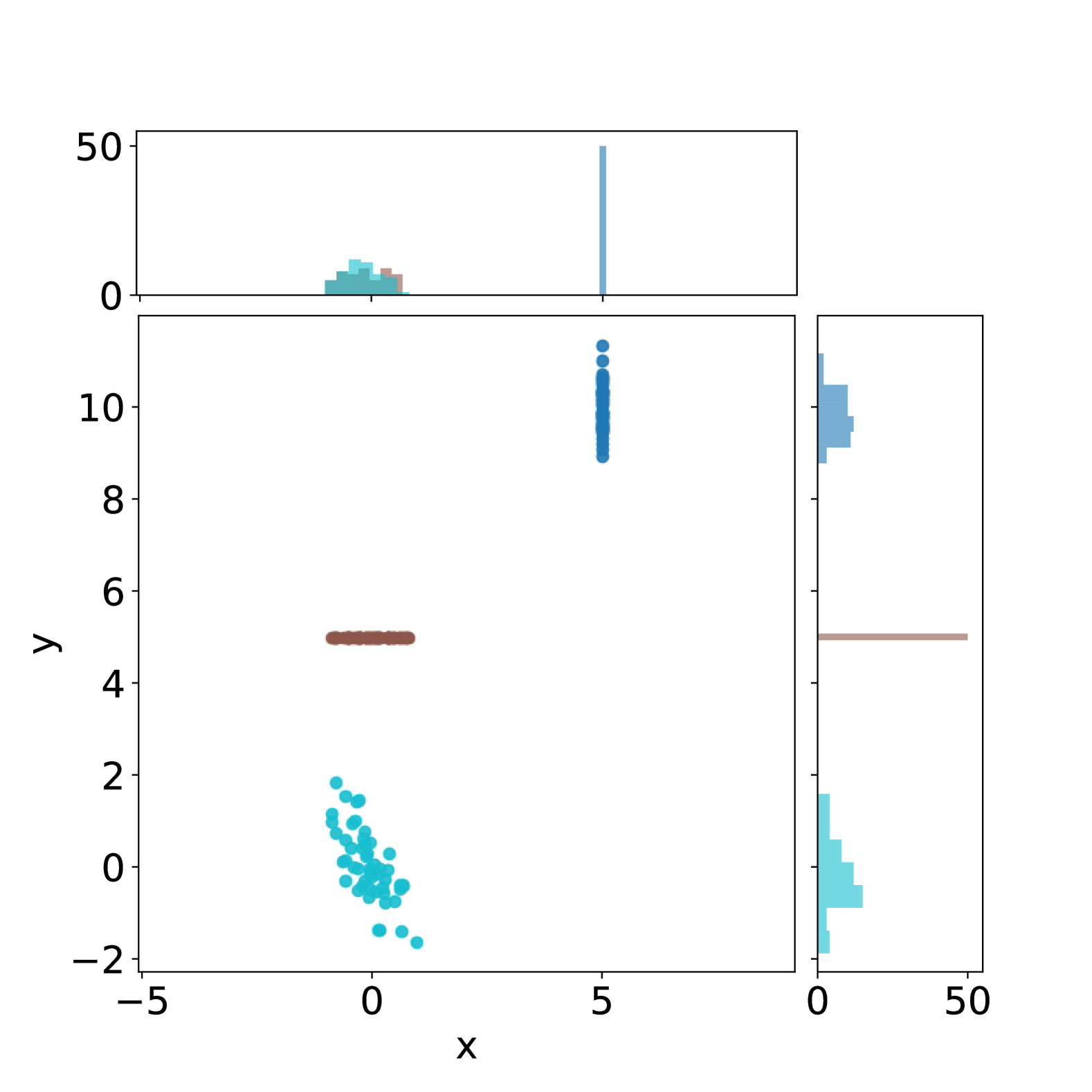
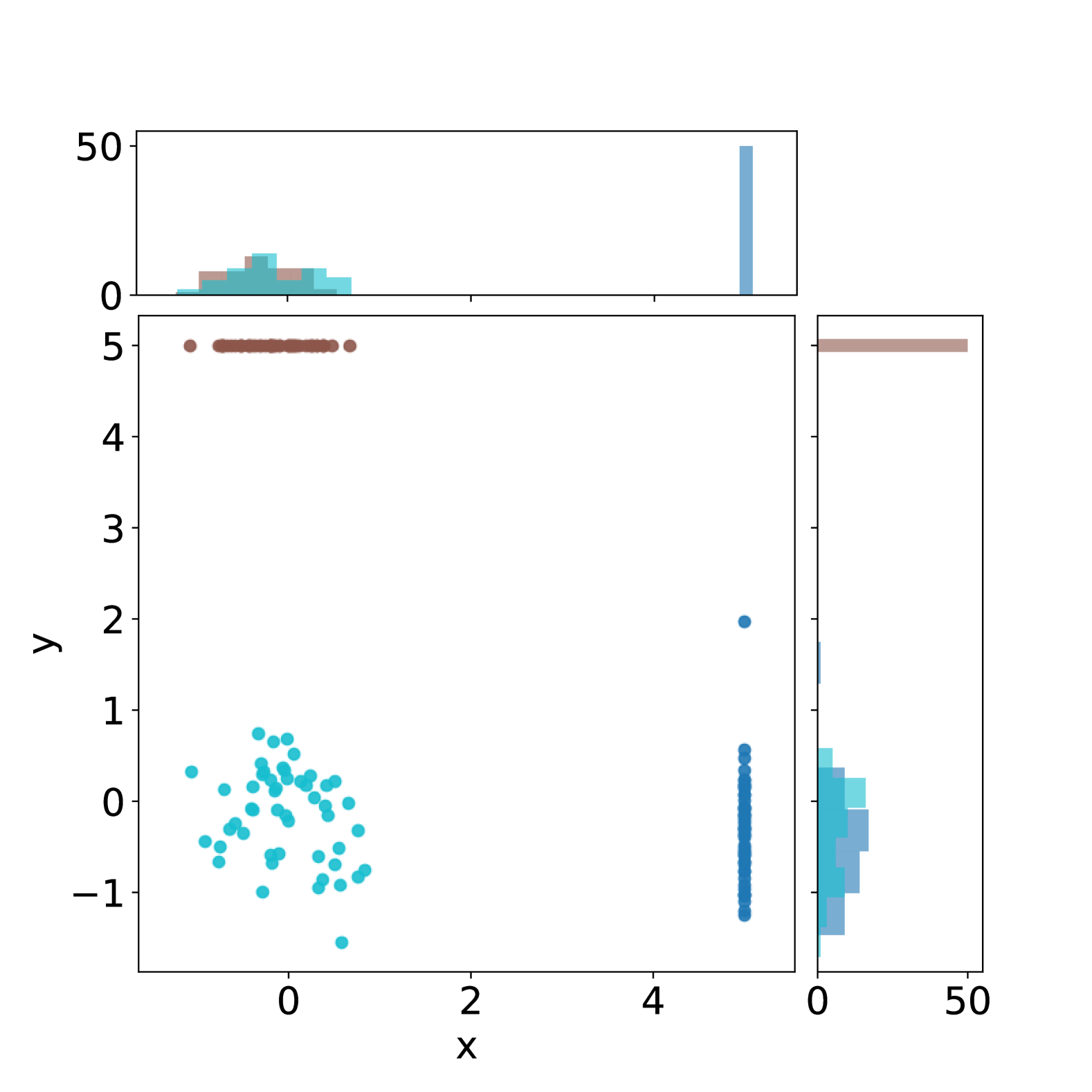
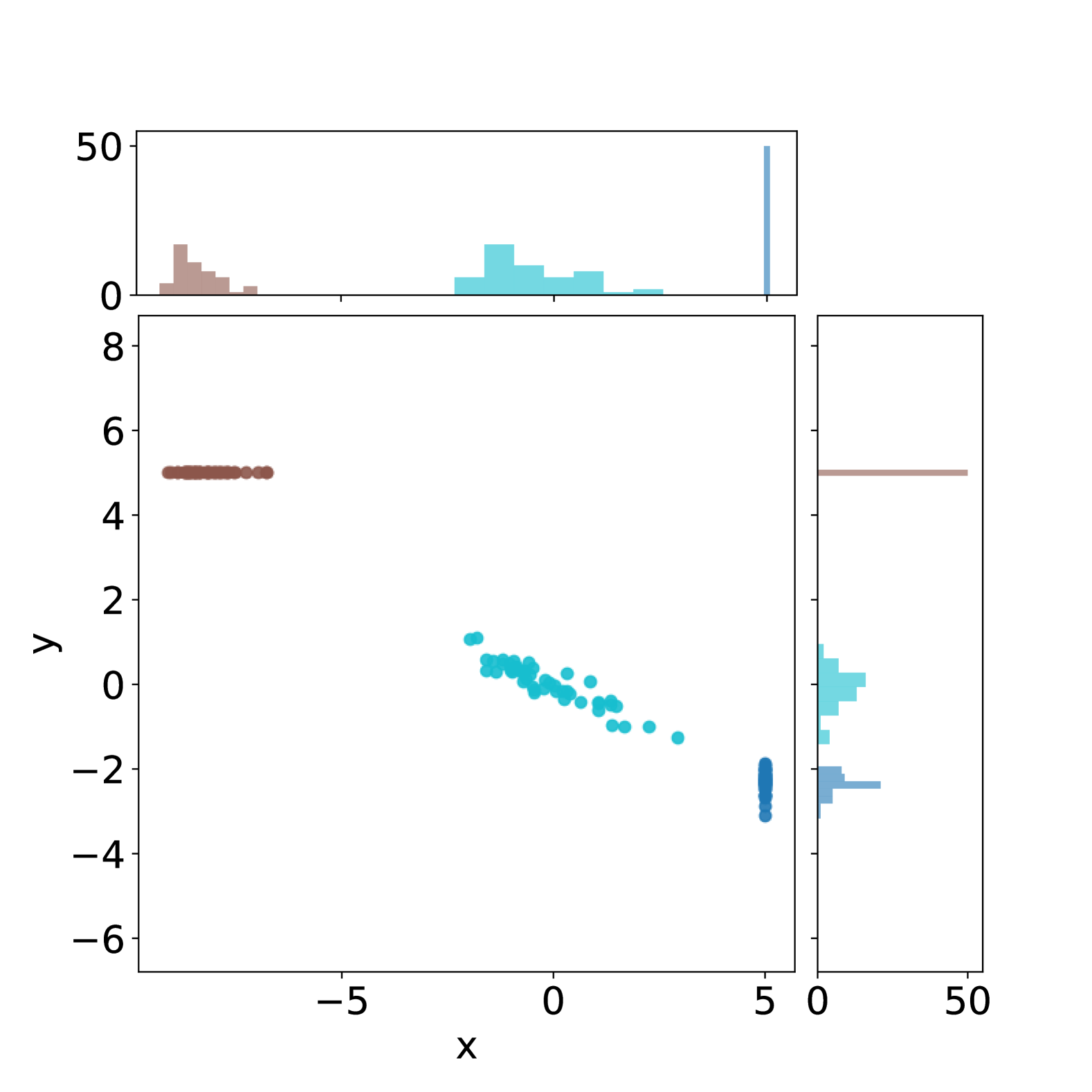
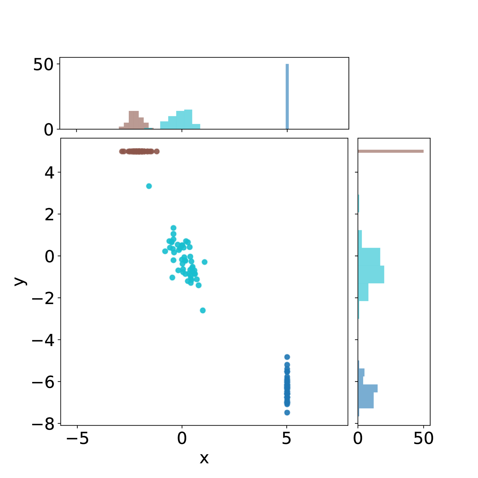
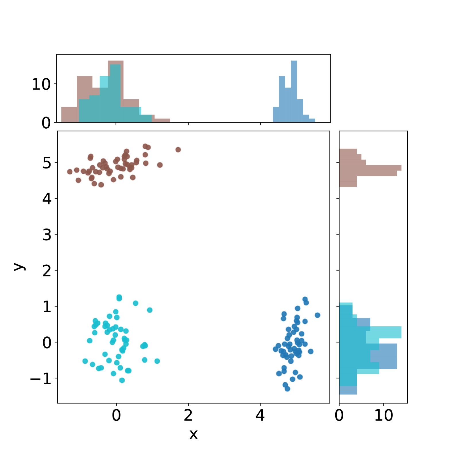
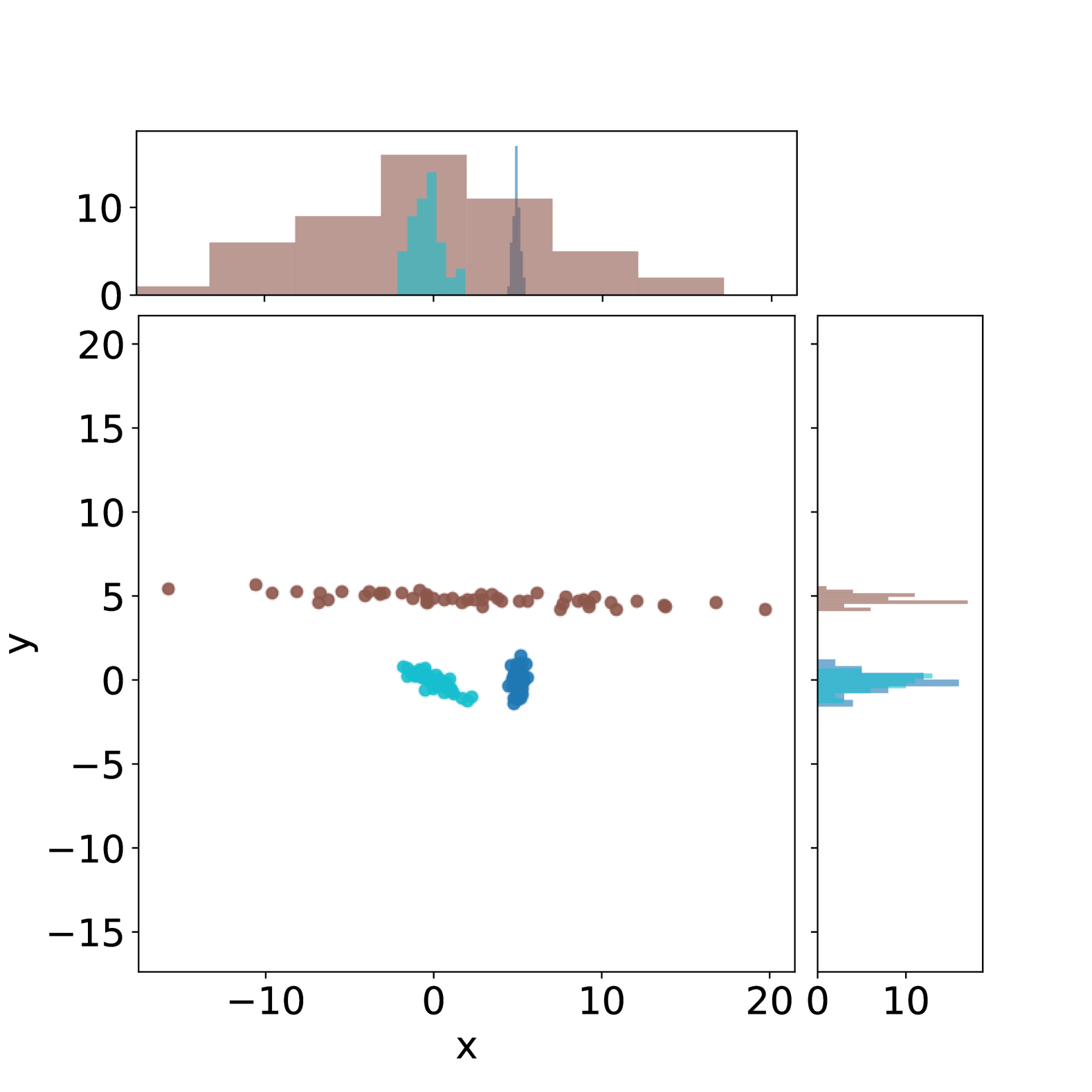
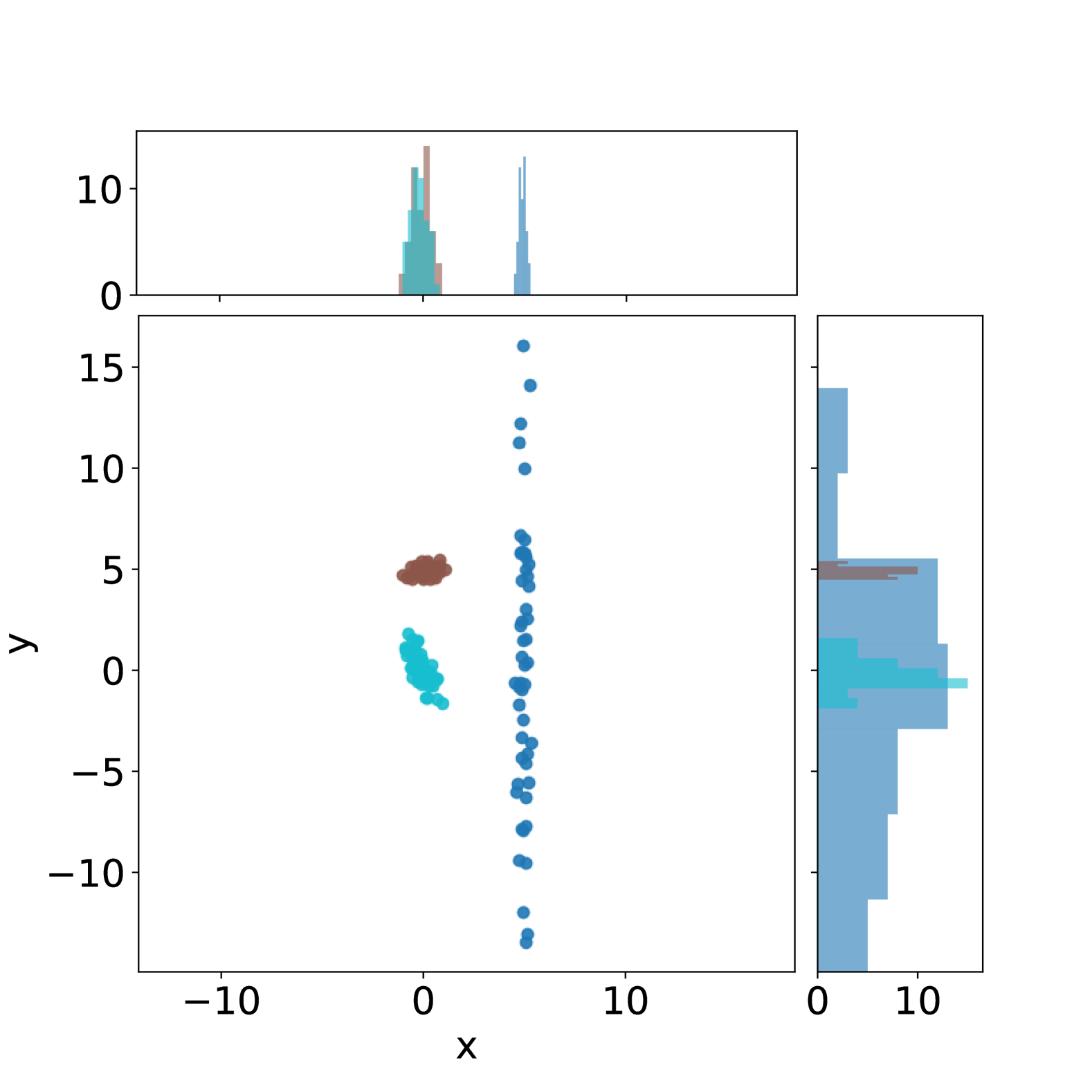
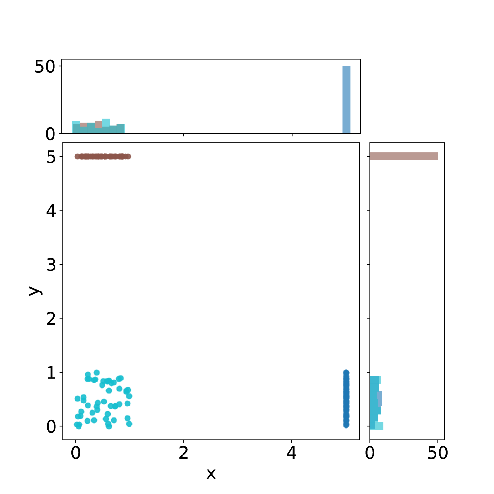
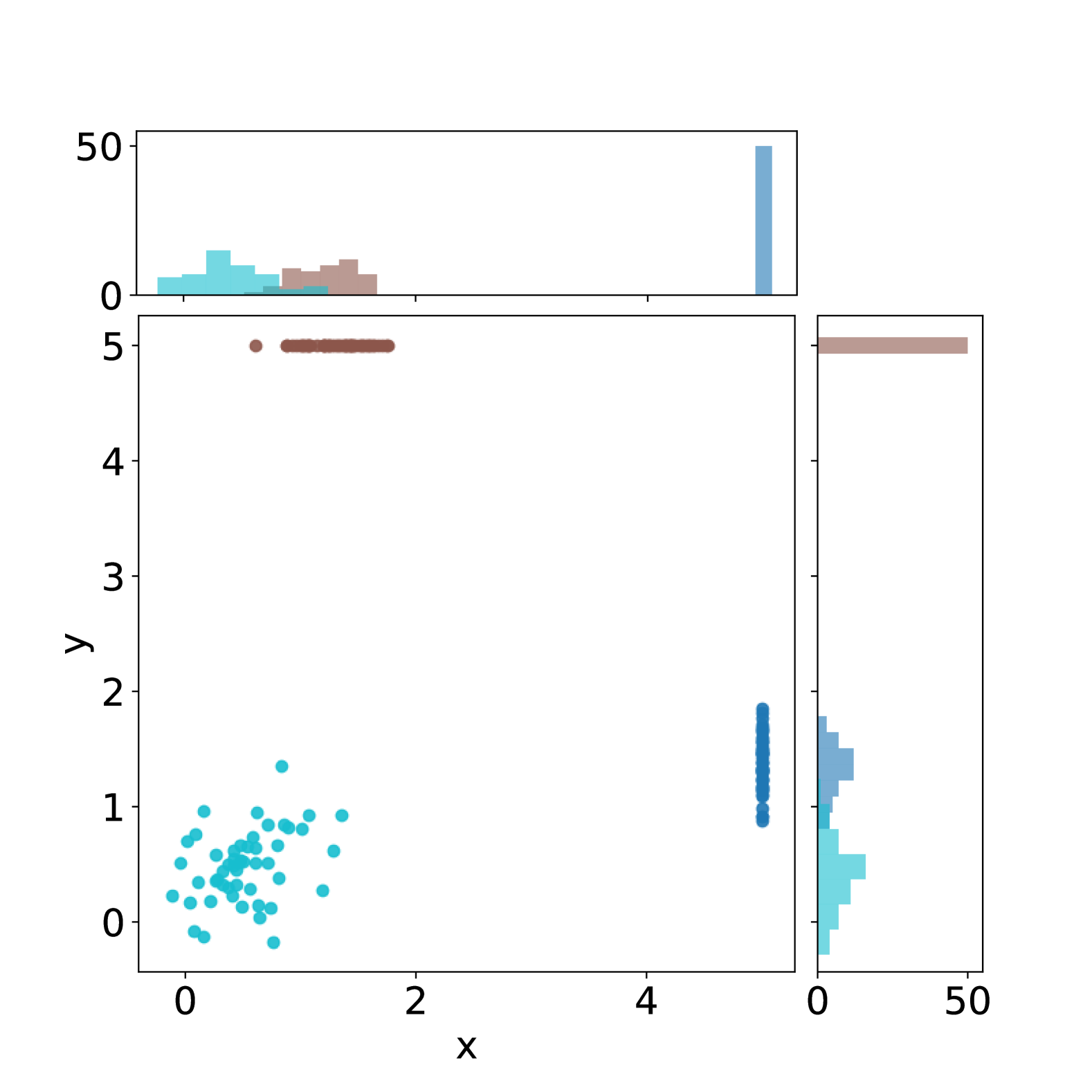
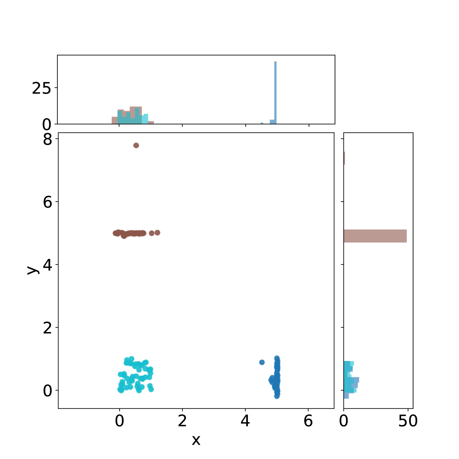
Figure 3 provides a qualitative view of the learned models on the held-out test Beta dataset. In this example, there is no causal effect between and . The turquoise points represent samples from the observational distribution, while the blue and brown points depict samples drawn from the interventional distributions by intervening on and (setting them to 5).
We see that conditioning alone shifts the mean of both interventional distributions, although no causal effect is present. For example, note how the distribution of (brown points) shifts when conditioned on , even though, according to the ground-truth model, it should remain unchanged. In contrast, our method correctly learns the underlying causal structure, preventing these erroneous shifts. Similar results appear in additional experiments for both the Beta and Gaussian test sets, shown in Figures 4 and 5 in the Appendix.
Conclusion.
These results indicate that our method successfully leverages causal information during inference. By performing a single forward pass at test time, the model estimates accurate interventional distributions that respect the true causal mechanisms governing the data-generating process, even for unseen test data.
4.5 Performance on Semi-Synthetic Data
To evaluate our method on data that more closely resembles real-world scenarios, we employ the SERGIO (Dibaeinia & Sinha, 2020) simulator for generating gene expression data. Following the setup in (Lorch et al., 2022), we create training and test sets using a fixed set of simulator parameters, as well as an out-of-distribution (OOD) evaluation dataset with a different set of parameters. In all datasets, the intervention corresponds to a gene-knockout experiment on one of the possible genes. Appendix A.2 provides the full list of hyperparameters used in this experiment.
Table 3 presents the results of our trained model and the baseline on both the test set and the OOD evaluation set, reporting the average performance metrics over the respective datasets.The results largely align with the ones found in Section 4.4, with the exception the estimated distributions now significantly differ from the ground truth. Still, the slightly higher -values for ACTIVA imply that its generated samples may deviate less from the ground truth overall.
| MMD | WSD | ERG | P | ||
|---|---|---|---|---|---|
| test | baseline | .50 | 5.07 | 3.49 | .0003 |
| ACTIVA | .32 | 6.19 | 2.08 | .004 | |
| ood | baseline | .63 | 8.36 | 8.62 | .001 |
| ACTIVA | .40 | 10.60 | 4.87 | .004 |
We also observe that performance degrades on the OOD data for both ACTIVA and the baseline. However, in addition to reflecting more challenging conditions, this decrease is partly confounded by the fact that the metrics are sensitive to data scale as detailed in Appendix B. Hence, changes in scale between the test (mean value 2.16) and OOD dataset (mean value 3.71) can amplify discrepancies in the reported metrics, even without a reduction in model performance.
Conclusion.
ACTIVA exhibits robust performance on unseen semi-synthetic data, confirming its applicability to more realistic domains. Furthermore, ACTIVA remains effective even under distribution shifts, highlighting its potential for handling OOD scenarios. ACTIVA’s advantage over the conditional baseline on semi-synthetic OOD data further highlights the benefits of its causal architecture in more accurately estimating interventional distributions and its potential transfer from simulated training data to real-world test data.
5 Related Work
Deep learning methods for causal inference have made progress in modeling observational, interventional, and counterfactual distributions. Some methods utilize variational autoencoders to learn latent causal representations for high-dimensional inputs, often assuming knowledge of the causal graph or learning the causal graph (Yang et al., 2021; Qi & Yu, 2023). Diffusion-based approaches train separate generative models for each variable and require graph structures upfront (Sanchez et al., 2022; Chao et al., 2023). Other methods leverage graph neural networks or normalizing flows to model causal relations but depend heavily on predefined graphs (Zečevi et al., 2021; Sánchez-Martin et al., 2022; Javaloy et al., 2023; Poinsot et al., 2024).
Joint inference methods estimate both graph structures and causal mechanisms, but typically require retraining (Lorch et al., 2021; Nishikawa-Toomey et al., 2022; Deleu et al., 2023). Other approaches focus on estimating treatment-outcome relationships without modeling the whole distribution (Louizos et al., 2017; Vowels et al., 2021; Wu & Fukumizu, 2023), require dataset-specific retraining (Khemakhem et al., 2021; Melnychuk et al., 2023) or are limited to specific classes of causal models (Cundy et al., 2021). Some approaches focus on special cases, such as limited overlap or marginal interventional data, but cannot handle joint distributions across all variables (Vanderschueren et al., 2023; Garrido et al., 2024).
Recently, (Mahajan et al., 2024) explored zero-shot learning for causal inference. Their approach is restricted to additive noise models and relies on knowing the underlying causal graphs during training, restricting its applicability to real-world scenarios. In contrast, our approach amortizes causal models to directly predict the joint interventional distribution for any dataset via a single forward pass. This eliminates retraining and assumptions on the causal structure, providing a scalable, flexible solution for causal inference.
6 Conclusion
In this work, we proposed ACTIVA, a novel approach for amortized causal inference that directly predicts the interventional distribution from observational data without requiring the underlying causal graph. Our transformer-based method is both permutation equivariant and permutation invariant to variable and sample ordering, respectively, making it robust and scalable across different causal models. Furthermore, the ability to perform inference in a zero-shot manner allows ACTIVA to generalize to new datasets without retraining, making it particularly promising for many real-world applications where interventional data is scarce or unavailable.
Our experimental results demonstrate that ACTIVA accurately estimates interventional distributions across synthetic and semi-synthetic datasets. The model consistently outperforms a conditional baseline, showing its ability to capture causal relationships beyond conditioning. The results confirm that ACTIVA effectively amortizes over many causal models, providing reliable inference beyond simple point estimates even for previously unseen and OOD datasets.
Regarding the limitations, the accuracy of ACTIVA is inherently tied to the representativeness of the training data. If the training distribution does not sufficiently capture the diversity of causal models encountered during inference, the model’s predictions may still be suboptimal. Additionally, while our empirical results are promising, further theoretical work is needed to better understand the generalization properties of amortized causal learning and the conditions under which the learned representations faithfully capture underlying causal mechanisms.
Nevertheless, our work highlights the significance of amortized causal inference as a scalable alternative to traditional approaches. By leveraging the expressivity of deep generative architectures, ACTIVA represents a step toward more flexible, efficient, and broadly applicable causal reasoning. Future research directions include extending the method to handle more complex scenarios and exploring connections between amortized inference and causal identifiability. We hope this work inspires further developments in rethinking causal inference in an amortized learning context with both theoretical and practical advances.
Impact Statement
This paper presents work whose goal is to advance the field of Machine Learning. There are many potential societal consequences of our work, none of which we feel must be specifically highlighted here.
Acknowledgments
We thank Frank van Harmelen, Emile van Krieken, Majid Mohammadi and Álvaro Serra-Gómez for their helpful inputs to this project.
This research was partially funded by the Hybrid Intelligence Center, a 10-year programme funded by the Dutch Ministry of Education, Culture and Science through the Netherlands Organisation for Scientific Research, https://hybrid-intelligence-centre.nl, grant number 024.004.022
References
- Annadani et al. (2025) Annadani, Y., Tigas, P., Bauer, S., and Foster, A. Amortized Active Causal Induction with Deep Reinforcement Learning. Advances in Neural Information Processing Systems, 37:44216–44239, 1 2025. URL https://arxiv.org/abs/2405.16718v1.
- Bareinboim et al. (2022) Bareinboim, E., Correa, J. D., Ibeling, D., and Icard, T. On Pearl’s Hierarchy and the Foundations of Causal Inference. Probabilistic and Causal Inference, pp. 507–556, 2 2022. doi: 10.1145/3501714.3501743. URL https://dl.acm.org/doi/10.1145/3501714.3501743.
- Chao et al. (2023) Chao, P., Blöbaum, P., Prasad, S., and Amazon, K. Interventional and Counterfactual Inference with Diffusion Models. arXiv preprint, 2023. URL https://github.com/patrickrchao/.
- Cundy et al. (2021) Cundy, C., Grover, A., and Ermon, S. BCD Nets: Scalable Variational Approaches for Bayesian Causal Discovery. Advances in Neural Information Processing Systems, 34:7095–7110, 12 2021.
- Deleu et al. (2023) Deleu, T., Nishikawa-Toomey, M., Subramanian, J., Malkin, N., Charlin, L., and Bengio, Y. Joint Bayesian Inference of Graphical Structure and Parameters with a Single Generative Flow Network. In Oh, A., Neumann, T., Globerson, A., Saenko, K., Hardt, M., and Levine, S. (eds.), Advances in Neural Information Processing Systems, volume 36, pp. 31204–31231. Curran Associates, Inc., 2023.
- Dibaeinia & Sinha (2020) Dibaeinia, P. and Sinha, S. SERGIO: A Single-Cell Expression Simulator Guided by Gene Regulatory Networks. Cell Systems, 11(3):252–271, 9 2020. ISSN 2405-4712. doi: 10.1016/J.CELS.2020.08.003.
- Dozat (2016) Dozat, T. Incorporating Nesterov Momentum into Adam, 2 2016.
- Garreau et al. (2017) Garreau, D., Jitkrittum, W., and Kanagawa, M. Large sample analysis of the median heuristic. 7 2017. URL https://arxiv.org/abs/1707.07269v3.
- Garrido et al. (2024) Garrido, S., Kirschbaum, E., Kekic, A., and Mastakouri, A. Estimating Joint interventional distributions from marginal interventional data. 9 2024. URL http://arxiv.org/abs/2409.01794.
- Gretton et al. (2012) Gretton, A., Borgwardt, K. M., Rasch, M. J., Smola, A., Schölkopf, B., and Smola GRETTON, A. A Kernel Two-Sample Test. Journal of Machine Learning Research, 13(25):723–773, 2012. ISSN 1533-7928. URL http://jmlr.org/papers/v13/gretton12a.html.
- Higgins et al. (2017) Higgins, I., Matthey, L., Pal, A., Burgess, C., Glorot, X., Botvinick, M., Mohamed, S., and Lerchner, A. beta-VAE: Learning Basic Visual Concepts with a Constrained Variational Framework, 2 2017.
- Hollmann et al. (2025) Hollmann, N., Müller, S., Purucker, L., Krishnakumar, A., Körfer, M., Bin Hoo, S., Schirrmeister, R. T., and Hutter, F. Accurate predictions on small data with a tabular foundation model. Nature —, 637:319, 2025. doi: 10.1038/s41586-024-08328-6. URL https://doi.org/10.1038/s41586-024-08328-6.
- Javaloy et al. (2023) Javaloy, A., Sanchez-Martin, P., and Valera, I. Causal normalizing flows: from theory to practice. Advances in Neural Information Processing Systems, 36:58833–58864, 12 2023. URL https://github.com/psanch21/causal-flows.
- Khemakhem et al. (2021) Khemakhem, I., Monti, R. P., Leech, R., and Hyvärinen, A. Causal Autoregressive Flows, 3 2021. ISSN 2640-3498. URL https://proceedings.mlr.press/v130/khemakhem21a.html.
- Kingma & Welling (2013) Kingma, D. P. and Welling, M. Auto-Encoding Variational Bayes. 2nd International Conference on Learning Representations, ICLR 2014 - Conference Track Proceedings, 12 2013. doi: 10.61603/ceas.v2i1.33. URL https://arxiv.org/abs/1312.6114v11.
- Kossen et al. (2021) Kossen, J., Band, N., Lyle, C., Gomez, A. N., Rainforth, T., and Gal, Y. Self-Attention Between Datapoints: Going Beyond Individual Input-Output Pairs in Deep Learning. Advances in Neural Information Processing Systems, 34:28742–28756, 12 2021.
- Kumar et al. (2023) Kumar, S., Vivek, Y., Ravi, V., and Bose, I. Causal Inference for Banking Finance and Insurance A Survey. 7 2023. URL https://arxiv.org/abs/2307.16427v1.
- Lorch et al. (2021) Lorch, L., Rothfuss, J., Schölkopf, B., and Krause, A. DiBS: Differentiable Bayesian Structure Learning. Advances in Neural Information Processing Systems, 34:24111–24123, 12 2021. URL https://github.com/larslorch/dibs.
- Lorch et al. (2022) Lorch, L., Sussex, S., Rothfuss, J., Krause, A., and Schölkopf, B. Amortized Inference for Causal Structure Learning. In Koyejo, S., Mohamed, S., Agarwal, A., Belgrave, D., Cho, K., and Oh, A. (eds.), Advances in Neural Information Processing Systems, volume 35, pp. 13104–13118. Curran Associates, Inc., 2022.
- Louizos et al. (2017) Louizos, C., Shalit, U., Mooij, J. M., Sontag, D., Zemel, R., and Welling, M. Causal Effect Inference with Deep Latent-Variable Models. Advances in Neural Information Processing Systems, 30, 2017.
- Mahajan et al. (2024) Mahajan, D., Gladrow, J., Hilmkil, A., Zhang, C., and Scetbon, M. Zero-Shot Learning of Causal Models. arXiv preprint, 2024.
- Marbach et al. (2009) Marbach, D., Schaffter, T., Mattiussi, C., and Floreano, D. Generating realistic in silico gene networks for performance assessment of reverse engineering methods. Journal of computational biology : a journal of computational molecular cell biology, 16(2):229–239, 2009. ISSN 1557-8666. doi: 10.1089/CMB.2008.09TT. URL https://pubmed.ncbi.nlm.nih.gov/19183003/.
- Melnychuk et al. (2023) Melnychuk, V., Frauen, D., and Feuerriegel, S. Normalizing Flows for Interventional Density Estimation. In International Conference on Machine Learning, pp. 24361–24397, 2023. URL https://github.com/.
- Nishikawa-Toomey et al. (2022) Nishikawa-Toomey, M., Deleu, T., Subramanian, J., Bengio, Y., and Charlin, L. Bayesian learning of Causal Structure and Mechanisms with GFlowNets and Variational Bayes. 11 2022. URL https://arxiv.org/abs/2211.02763v3.
- Panizza & Presbitero (2014) Panizza, U. and Presbitero, A. F. Public debt and economic growth: Is there a causal effect? Journal of Macroeconomics, 41:21–41, 9 2014. ISSN 0164-0704. doi: 10.1016/J.JMACRO.2014.03.009.
- Peters et al. (2017) Peters, J., Janzig, D., and Schölkopf, B. Elements of causal inference: foundations and learning algorithms. The MIT Press, 2017.
- Poinsot et al. (2024) Poinsot, A., Leite, A., Chesneau, N., Sébag, M., and Schoenauer, M. Learning Structural Causal Models through Deep Generative Models: Methods, Guarantees, and Challenges. arXiv preprint, 2024.
- Qi & Yu (2023) Qi, G. and Yu, H. CMVAE: Causal Meta VAE for Unsupervised Meta-Learning. Proceedings of the AAAI Conference on Artificial Intelligence, 37(8):9480–9488, 6 2023. ISSN 2374-3468. doi: 10.1609/AAAI.V37I8.26135. URL https://ojs.aaai.org/index.php/AAAI/article/view/26135.
- Rissanen & Marttinen (2021) Rissanen, S. and Marttinen, P. A Critical Look at the Identifiability of Causal Effects with Deep Latent Variable Models. In Conference on Neural Information Processing Systems, 2021.
- Sanchez et al. (2022) Sanchez, P., Tsaftaris, S. A., Schölkopf, B., Uhler, C., and Zhang, K. Diffusion Causal Models for Counterfactual Estimation, 6 2022. ISSN 2640-3498. URL https://proceedings.mlr.press/v177/sanchez22a.html.
- Sánchez-Martin et al. (2022) Sánchez-Martin, P., Rateike, M., and Valera, I. VACA: Designing Variational Graph Autoencoders for Causal Queries. Proceedings of the AAAI Conference on Artificial Intelligence, 36(7):8159–8168, 6 2022. ISSN 2374-3468. doi: 10.1609/AAAI.V36I7.20789. URL https://ojs.aaai.org/index.php/AAAI/article/view/20789.
- Sauter et al. (2024a) Sauter, A., Acar, E., and Plaat, A. CausalPlayground: Addressing Data-Generation Requirements in Cutting-Edge Causality Research. arXiv preprint, 2024a.
- Sauter et al. (2024b) Sauter, A. W. M., Botteghi, N., Acar, E., and Plaat, A. CORE: Towards Scalable and Efficient Causal Discovery with Reinforcement Learning. Proceedings of the 23rd International Conference on Autonomous Agents and Multiagent Systems (AAMAS), pp. 1664–1672, 2024b.
- Scetbon et al. (2024) Scetbon, M., Jennings, J., Hilmkil, A., Zhang, C., and Ma, C. A Fixed-Point Approach for Causal Generative Modeling, 2024.
- Shi & Norgeot (2022) Shi, J. and Norgeot, B. Learning Causal Effects From Observational Data in Healthcare: A Review and Summary. Frontiers in Medicine, 9:864882, 7 2022. ISSN 2296858X. doi: 10.3389/FMED.2022.864882/BIBTEX. URL www.frontiersin.org.
- Sohn et al. (2015) Sohn, K., Yan, X., and Lee, H. Learning Structured Output Representation using Deep Conditional Generative Models. Advances in Neural Information Processing Systems, 2015.
- Székely & Rizzo (2013) Székely, G. J. and Rizzo, M. L. Energy statistics: A class of statistics based on distances. Journal of Statistical Planning and Inference, 143(8):1249–1272, 8 2013. ISSN 0378-3758. doi: 10.1016/J.JSPI.2013.03.018.
- Tomczak & Welling (2018) Tomczak, J. M. and Welling, M. VAE with a VampPrior. In International conference on artificial intelligence and statistics. PMLR, pp. 1214–1223, 2018.
- Vanderschueren et al. (2023) Vanderschueren, T., Berrevoets, J., Verbeke, W., and Leuven, K. U. NOFLITE: Learning to Predict Individual Treatment Effect Distributions. Transactions on Machine Learning Research, 2023.
- Vaswani et al. (2017) Vaswani, A., Brain, G., Shazeer, N., Parmar, N., Uszkoreit, J., Jones, L., Gomez, A. N., Kaiser, L., and Polosukhin, I. Attention Is All You Need. In Advances in Neural Information Processing Systems, 2017.
- Villani (2009) Villani, C. Optimal Transport. 338, 2009. doi: 10.1007/978-3-540-71050-9. URL http://link.springer.com/10.1007/978-3-540-71050-9.
- Vowels et al. (2021) Vowels, M. J., Cihan Camgoz, N., and Bowden, R. Targeted VAE: Variational and Targeted Learning for Causal Inference. IEEE International Conference on Smart Data Services, 2021. doi: 10.1109/SMDS53860.2021.00027. URL https://github.com/matthewvowels1/TVAE.
- Wu & Fukumizu (2023) Wu, P. and Fukumizu, K. -Intact-VAE: Identifying and Estimating Causal Effects under Limited Overlap. International Conference on Learning Representation, 2023.
- Yang et al. (2021) Yang, M., Liu, F., Chen, Z., Shen, X., Hao, J., and Wang, J. CausalVAE: Disentangled Representation Learning via Neural Structural Causal Models. Proceedings of the IEEE/CVF Conference on Computer Vision and Pattern Recognition (CVPR), 2021.
- Zečevi et al. (2021) Zečevi, M., Singh Dhami, D., Veličkovi, P., and Kersting KERSTING, K. Relating Graph Neural Networks to Structural Causal Models. arXiv preprint, 2021. URL https://anonymous.4open.science/r/.
Appendix A Datasets
We evaluate the performance of the proposed method across three different types of datasets: two purely synthetic (Gaussian and Beta) and one semi-synthetic (SERGIO). Below, we provide an overview of each dataset category along with the relevant parameters. For every causal model in these categories, we draw samples from both the observational and the interventional distributions to create paired datasets. Details about the exact number of models, how we split into training/test sets, and further parameter choices are given in the subsections below.
A.1 Synthetic Data (Gaussian and Beta Noise)
We generate data from linear additive causal models of the form:
where is drawn from either: A Gaussian distribution, , or A Beta distribution, . For each variable , we generate interventional data by applying a single-variable intervention . In total, this yields one observational dataset and interventional dataset for each causal model. All synthetic data is generated with the Causal Playground library (Sauter et al., 2024a).
When the noise terms follow a Gaussian distribution, we sample uniformly from and let . For the Beta case, we again draw in , but the noise terms follow with .
We examine both a 2-variable and an 8-variable scenario:
-
•
Two Variables. We randomly generate 6000 linear models using 3 distinct causal graphs (e.g., , , or no edges) and sample 50 points each for the observational and interventional distributions. We split these 6000 models into 5400 for training and 600 for testing.
-
•
Eight Variables. We generate 30,000 linear models (with 2000 distinct graphs, each instantiated with different parameters). For each model, we sample 30 data points for the observational and for each interventional distribution. Of these 30,000 models, 27,000 are used for training and 3000 are held out for testing.
A.2 Semi-Synthetic Data (SERGIO)
To evaluate on data with biological realism, we employ the SERGIO simulator (Dibaeinia & Sinha, 2020), which generates single-cell gene-expression data. Notably, we use the version of SERGIO provided in (Lorch et al., 2022), which includes functionality for performing interventions. We treat single-gene knockouts as interventions, thus applying to each gene . This yields one observational dataset and 11 single-gene interventional datasets per simulated gene-regulatory network.
Simulator Settings and Network Structures.
Following the procedure in (Marbach et al., 2009; Lorch et al., 2021), we randomly sample subgraphs of known gene-regulatory networks from E. coli or S. cerevisiae, ensuring that each subgraph has 11 genes. For each subgraph, we draw model parameters (e.g., activation constants, decay rates, and noise magnitudes) from predefined ranges. We then generate observational data as well as data from each gene-knockout intervention.
Training, Testing, and Out-of-Distribution (OOD) Splits.
We run 15,000 SERGIO simulations for our in-distribution dataset and sample 30 cells (data points) for each observational and interventional condition. We then split these 15,000 simulations into training (90%) and test (10%). We also construct an OOD set of 1800 simulations, where some SERGIO parameters (e.g., noise or decay rates) are sampled from partially disjoint ranges, creating a controlled distribution shift. For evaluation, we again sample 30 cells per observational/interventional condition in these OOD simulations.
In summary, the synthetic datasets allow us to systematically analyze the ability of our amortized approach to capture linear causal effects under distinct noise assumptions, while the semi-synthetic SERGIO datasets bring our method closer to real-world conditions by simulating biologically realistic gene-expression data under interventions.
| parameter | in-distribution | out-of-distribution |
|---|---|---|
| b | Uniform(0, 1) | Uniform(0.5, 2.0) |
| k_param | Uniform(1, 5) | Uniform(3, 7) |
| k_sign | Beta(1, 1) | Beta(0.5, 0.5) |
| hill | { 1.9, 2.0, 2.1} | { 1.5, 2.5} |
| decays | { 0.7, 0.8, 0.9} | { 0.5, 1.5} |
| noise_params | {0.9, 1.0, 1.1} | {0.5, 1.5} |
Appendix B Metrics
To quantitatively assess how closely our estimated interventional distributions align with the ground-truth or observed distributions, we employ three sample-based distance measures and a permutation-based statistical test. Specifically, we use:
-
•
Maximum Mean Discrepancy (MMD)
-
•
Wasserstein Distance (WSD)
-
•
Energy Distance (ERG)
-
•
Energy-Based Permutation Test
Each of these distances captures a distinct notion of distributional similarity. The MMD is a kernel-based embedding measure that detects differences in distribution means in a reproducing kernel Hilbert space; the Wasserstein distance considers a geometric “transport cost” viewpoint; the energy distance focuses on pairwise distance comparisons; and the permutation test provides a statistical criterion for whether two sets of samples could plausibly come from the same underlying distribution. Taken together, these four methods give a robust picture of how well our learned distributions match the ground truth in terms of shape, location, and higher-order moments.
Maximum Mean Discrepancy (MMD).
The MMD (Gretton et al., 2012) compares the mean embeddings of two distributions, and , in a reproducing kernel Hilbert space (RKHS). Concretely, for samples and , MMD is computed as:
where is a positive-definite kernel. Lower MMD values indicate that the two sets of samples are more similar with respect to that kernel-induced feature map. In our experiments, we use a Gaussian (RBF) kernel
whose bandwidth parameter is chosen via the median heuristic (i.e., by setting the kernel scale to the median distance among all pairs of training samples). This approach is a common, adaptive way to select an appropriate kernel width without extensive hyperparameter tuning (Garreau et al., 2017).
Wasserstein Distance (WSD).
Also referred to as the Earth Mover’s Distance, the Wasserstein distance (Villani, 2009) evaluates how much “effort” is needed to transform one distribution into another. Formally, for :
where is the set of all couplings of and , and is a distance metric (usually Euclidean). A lower Wasserstein distance indicates that the two distributions are closer in a geometric sense, reflecting both differences in location and in spread.
Energy Distance (ERG).
The energy distance (Székely & Rizzo, 2013) offers yet another perspective on distributional similarity by comparing pairwise distances:
where and . Lower energy distance values indicate higher overall similarity between and in terms of both mean locations and dispersion patterns.
Energy-Based Permutation Test.
Finally, we apply a permutation test based on the energy distance to determine whether two sets of samples are statistically indistinguishable from one another. Specifically, we first compute the observed energy distance between the real (or ground-truth) samples and the model-generated samples. Then we pool the two sets of samples and repeatedly sample 100 random permutations to split them into two groups of the original sizes. Finally we compute the energy distance for each permutation, thereby approximating a null distribution in which and are “mixed.”
If is not significantly larger than typical values (at a chosen significance level), we fail to reject the null hypothesis that both sets of samples come from the same distribution. Hence, a high -value indicates that our learned samples are statistically indistinguishable from the ground truth.
Appendix C Hyperparameters
Table 5 provides a summary of the principal hyperparameters used in our experiments, along with their chosen values for each model variant.
Models and Experiments.
-
•
Gaussian and Beta refer to the models used in the bivariate experiments described in Section 4.4.
-
•
Gaussian 1 and Gaussian 10 are two versions of our architecture (with single-component and 10-component Gaussian output mixtures, respectively) used in the eight-variable experiments on Gaussian data.
-
•
Beta 1 and Beta 10 analogously represent single-component and 10-component mixture versions for the eight-variable Beta-noise experiments (see Appendix D.1 for results).
-
•
SERGIO is the version of our model employed for the semi-synthetic gene-expression data of the experiment in Section 4.5).
Explanation of Table Columns.
-
•
Batch size indicates how many datasets are processed in each training step.
-
•
Heads is the number of heads used in the multi-head self-attention layers.
-
•
K (in our table notation) specifies the number of Transformer blocks used in the decoder.
-
•
Dropout is the probability of randomly dropping units in the attention and feed-forward sublayers.
-
•
e indicates the embedding dimension for each feature before attention is applied.
-
•
d is the dimensionality of input features.
-
•
c denotes the number of Gaussian components used in the mixture for the decoder’s output distribution.
-
•
L is the number of Transformer blocks in the encoder, alternating attention over sample and feature axes. This always has to be an even number.
-
•
epochs is the total number of passes through the training dataset.
-
•
lr is the learning rate used for the Adam-based optimizer (Dozat, 2016).
-
•
seed ensures reproducibility of parameter initialization and dataset splits.
-
•
is the coefficient that balances the KL term in our -VAE training objective (see Section 4 of the main text). A value less than 1 places more emphasis on accurate reconstruction over disentanglement.
| batch size | heads | K | dropout | e | d | c | L | epochs | lr | seed | ||
|---|---|---|---|---|---|---|---|---|---|---|---|---|
| Gaussian | 1800 | 6 | 2 | 0.1 | 16 | 2 | 10 | 4 | 20000 | 0.001 | 42 | 0.01 |
| Gaussian 1 | 350 | 6 | 2 | 0.1 | 16 | 8 | 1 | 4 | 10000 | 0.001 | 42 | 0.0005 |
| Gaussian 10 | 350 | 6 | 2 | 0.1 | 16 | 8 | 10 | 4 | 9650 | 0.001 | 42 | 0.0005 |
| Beta | 1800 | 6 | 2 | 0.1 | 16 | 2 | 10 | 4 | 20000 | 0.001 | 42 | 0.005 |
| Beta 1 | 350 | 6 | 2 | 0.1 | 16 | 8 | 1 | 4 | 10000 | 0.001 | 42 | 0.0005 |
| Beta 10 | 350 | 6 | 2 | 0.1 | 16 | 8 | 10 | 4 | 9650 | 0.001 | 42 | 0.0005 |
| SERGIO | 256 | 8 | 2 | 0.1 | 16 | 8 | 15 | 4 | 20000 | 0.0005 | 42 | 0.005 |
All runs were performed on an NVIDIA A6000 GPU, except for the SERGIO model, which was trained on an NVIDIA A100. Training times vary depending on model size (d, e, c) and dataset size (batch size, epochs). Larger mixture components () and higher embedding dimensions () generally increase both training time and representational capacity. Potential NaN’s in the optimization are zeroed.
In summary, the hyperparameters in Table 5 reflect our balancing of model complexity, regularization, and computational resource constraints. Values are chosen empirically to ensure stable training and satisfactory performance across different experimental settings.
Appendix D Additional Results
In this section, we provide further experimental results that complement those presented in the main paper. We first show additional quantitative comparisons for Beta-noise models with 8 variables, and then include extended visualizations of bivariate predictions for both Beta and Gaussian data.
D.1 More Results on Beta-Noise Models
Table 6 reports the inference performance of two versions of our model, Beta 1 and Beta 10, evaluated on 3000 previously unseen test causal models with 8 variables each. These models differ only in the number of Gaussian mixture components ( vs. ) used to parameterize the decoder output. As in the main text, we compare against the conditional baseline that fits a single multivariate normal to observational data and then conditions on the intervened variables.
| mmd | wsd | erg | p | |
|---|---|---|---|---|
| Baseline | .94 | 10.90 | 18.52 | .00 |
| Beta 1 | .59 | 14.85 | 12.44 | .00 |
| Beta 10 | .59 | 15.41 | 11.53 | .002 |
The comparison exhibits a similar pattern as the Gaussian-noise models:
-
•
MMD and ERG are substantially lower for both Beta 1 and Beta 10 than for the baseline, indicating that our method’s samples align more closely with the true interventional distributions in a kernel embedding and pairwise-distance sense.
-
•
The WSD is higher for both Beta 1 and Beta 10. We hypothesize that this is due to the model outputting broader variances in some directions, leading to higher “transport cost” under the Wasserstein metric.
-
•
The permutation test -value remains relatively low for all methods (including ours), suggesting some residual mismatch to the true distribution.
D.2 Visualizations of Bivariate Estimates
To complement our quantitative results, Figures 4 and 5 provide qualitative illustrations of the learned interventional distributions for bivariate models with either Beta or Gaussian additive noise. Each figure consists of four rows, each corresponding to a distinct data-generating process (or parameter configuration). In each subplot:
-
•
The left column (“Original”) shows samples from the ground-truth observational (turquoise) and interventional distributions (blue/brown).
-
•
The middle column (“Baseline”) shows reconstructed samples from conditioning on the intervened variables in a single fitted MVN.
-
•
The right column (“Model”) shows the corresponding draws from ACTIVA’s learned interventional distributions.
In Figures 4 and 5, we observe:
-
•
False Shifts in the Conditional Baseline. Conditioning alone often shifts non-target variables, even when there is no causal path. This is particularly visible for certain Beta-noise cases.
-
•
Correct Zero-Effect Modeling. ACTIVA preserves the distribution of non-target variables unless there is a true causal relationship, avoiding unnecessary changes.
-
•
Increased Variance. Our model sometimes outputs broader distributions, which can manifest in higher Wasserstein distance but still yield more faithful coverage of the true data-generating process.
Overall, these additional results reinforce our main findings. ACTIVA accurately captures causal asymmetries in both Beta and Gaussian noise settings and avoids the pitfall of naively “conditioning away” correlations to produce artifacts where no causal effect exists.