Robust Simulation-Based Inference
under Missing Data via Neural Processes

Abstract

Simulation-based inference (SBI) methods typically require fully observed data to infer parameters of models with intractable likelihood functions. However, datasets often contain missing values due to incomplete observations, data corruptions (common in astrophysics), or instrument limitations (e.g., in high-energy physics applications). In such scenarios, missing data must be imputed before applying any SBI method. We formalize the problem of missing data in SBI and demonstrate that naive imputation methods can introduce bias in the estimation of SBI posterior. We also introduce a novel amortized method that addresses this issue by jointly learning the imputation model and the inference network within a neural posterior estimation (NPE) framework. Extensive empirical results on SBI benchmarks show that our approach provides robust inference outcomes compared to standard baselines for varying levels of missing data. Moreover, we demonstrate the merits of our imputation model on two real-world bioactivity datasets (Adrenergic and Kinase assays). Code is available at https://github.com/Aalto-QuML/RISE.

1 Introduction

Mechanistic models for studying complex physical or biological phenomena have become indispensable tools in research fields as diverse as genetics (Riesselman et al., 2018), epidemiology (Kypraios et al., 2017), gravitational wave astronomy (Dax et al., 2021), and radio propagation (Bharti et al., 2022a). However, fitting such models to observational data can be challenging due to the intractability of their likelihood functions, which renders standard Bayesian inference methods inapplicable. Simulation-based inference (SBI) methods (Cranmer et al., 2020) tackle this issue by relying on forward simulations from the model instead of evaluating the likelihood. These simulations are then either used to train a conditional density estimator (Papamakarios and Murray, 2016; Lueckmann et al., 2017b; Greenberg et al., 2019; Papamakarios et al., 2019; Radev et al., 2020), or to measure distance with the observed data (Sisson, 2018; Briol et al., 2019; Pesonen et al., 2023), to approximately estimate the posterior distribution of the model parameters of interest.

SBI methods implicitly assume that the observed data distribution belongs to the family of distributions induced by the model; i.e., the model is well-specified. However, this assumption is often violated in practice where models tend to be misspecified since the complex real-world phenomena under study are not accurately represented. Even if the model is well-specified, the data collection mechanism might hinder the applicability of SBI methods since it can induce missing data due to, for instance, incomplete observations (Luken et al., 2021), instrument limitations (Kasak et al., 2024), or unfavorable experimental conditions.

Although the former problem of model misspecification has been studied in a number of works (Frazier et al., 2020; Dellaporta et al., 2022; Fujisawa et al., 2021; Bharti et al., 2022b; Ward et al., 2022; Schmitt et al., 2023; Gloeckler et al., 2023; Huang et al., 2023; Gao et al., 2023; Kelly et al., 2024), the latter problem of missing data in SBI has received relatively less attention. A notable exception is the work of Wang et al. (2024), which attempts to handle missing data by augmenting and imputing constant values (e.g., zero or sample mean) and performing inference with a binary mask indicator. However, this approach can lead to biased estimates, reduced variability, and distorted relationships between variables (Graham et al., 2007). This is exemplified in Figure˜1 where we investigate the impact of missing data on neural posterior estimation (NPE, Papamakarios and Murray (2016))—a popular SBI method—on a population genetics model. We observe that simply incorporating missing values and their corresponding masks in NPE methods as in Wang et al. (2024) leads to biased posterior estimates.

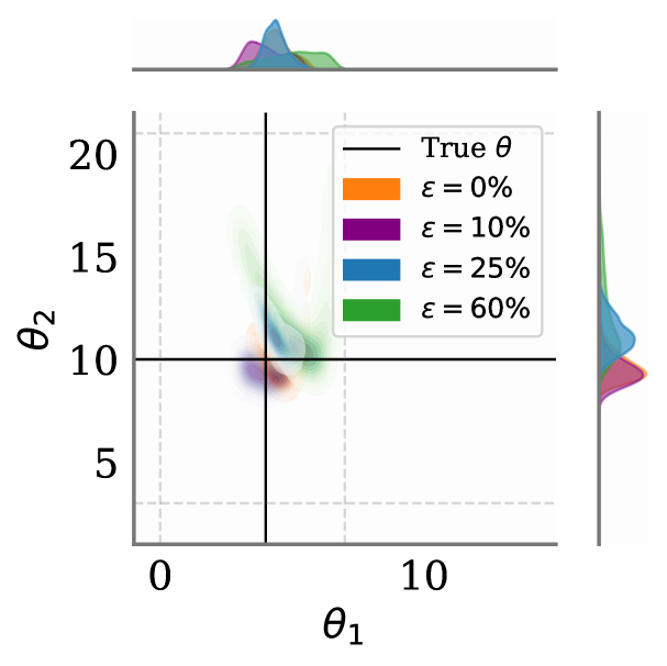
Figure 1: Effect of missing data on SBI. NPE posterior for the two-parameter Ricker model (Wood, 2010) where the method of Wang et al. (2024) (with zero augmentation) is used to handle $\varepsilon\%$ of values missing in the data. As $\varepsilon$ increases, the NPE posteriors become biased and drift away from the true parameter value, denoted by the black lines.

Other SBI works that address missing data include Lueckmann et al. (2017a) and Gloeckler et al. (2024), however, they fail to account for the underlying mechanism that leads to missing values in the data.

Outside of SBI, the problem of missing data has been extensively studied (Van Buuren and Groothuis-Oudshoorn, 2011), with Rubin (1976) categorizing it into three types: missing completely at random (MCAR), missing at random (MAR), and missing not at random (MNAR). Recent advances in machine learning have led to the development of novel methods for addressing this problem using generative adversarial networks (GANs, Luo et al. (2018); Yoon et al. (2018); Li et al. (2019); Yoon and Sull (2020)), variational autoencoders (VAEs, Nazabal et al. (2020); Collier et al. (2020); Mattei and Frellsen (2019); Ipsen et al. (2020); Ghalebikesabi et al. (2021b)), Gaussian processes (Casale et al., 2018; Fortuin et al., 2020; Ramchandran et al., 2021; Ong et al., 2024), and optimal transport (Muzellec et al., 2020; Zhao et al., 2023; Vo et al., 2024). These methods offer new perspectives on the problem of missing data imputation, but their application has been primarily limited to predicting missing values. Notably, they have not been developed for inference
over missing values, which remains a significant challenge for SBI.

Contributions.

In this paper, we introduce a novel SBI method that is robust to shift in the posterior distribution due to missing data. Our method, named RISE (short for “Robust Inference under imputed SimulatEd data”), jointly performs imputation and inference by combining NPE with latent neural processes (Foong et al., 2020). Doing so allows us to learn an amortized model unlike other robust SBI methods in the literature, and to handle missing data under different assumptions (Little and Rubin, 2019). We summarize our main contributions below:

• we motivate the problem of missing data in SBI, arguing how it can induce bias in posterior estimation;

• we propose RISE, an amortized method, that jointly learns an imputation and inference network to deal with missing data;

• RISE outperforms competing baselines in inference and imputation tasks across varying levels of missingness, demonstrating robust performance in settings entailing missing data.

2 Preliminaries

Consider a simulator-based model $p(\cdot\,|\,\theta)$ that takes in a parameter vector $\theta\in\Theta\subseteq\mathbb{R}^{p}$ and maps it to a point $\mathbf{x}=[x_{1},\dots,x_{d}]^{\top}$ in some data space $\mathcal{X}\subseteq\mathbb{R}^{d}$. We assume that $p(\cdot\,|\,\theta)$ is intractable, meaning that its associated likelihood function is unavailable and cannot be evaluated point-wise. However, in our setting, generating independent and identically distributed (iid) realisations $\mathbf{x}\sim p(\cdot\,|\,\theta)$ for a fixed $\theta$ is straightforward. Given a dataset $\tilde{\mathbf{x}}$ collected via real-world experiments from some true data-generating process and a prior distribution on the parameters $p(\theta)$, we are interested in approximating the posterior distribution $p(\theta\,|\,\tilde{\mathbf{x}})\propto p(\tilde{\mathbf{x}}\,|\,\theta)p(\theta)$. This can be achieved, for instance, using the popular neural posterior estimation (NPE) method, which we now introduce.

Neural posterior estimation.

NPE (Papamakarios and Murray, 2016) involves training conditional density estimators, such as normalizing flows (Papamakarios et al., 2021), to learn a mapping from each datum $\mathbf{x}$ to the posterior distribution $p(\theta\,|\,\mathbf{x})$. Specifically, we can approximate the posterior distribution with $q_{\phi}(\theta\,|\,\mathbf{x})$ using learnable parameters $\phi$. In particular, we can train $q_{\phi}$ by minimizing an empirical loss

$$\ell_{\mathrm{NPE}}(\phi)\triangleq-\frac{1}{n}\sum_{i=1}^{n}\log q_{\phi}(\theta_{i}\,|\,\mathbf{x}_{i})\approx-\mathbb{E}_{\theta\sim p(\theta)}[\mathbb{E}_{\mathbf{x}\sim p(\mathbf{x}\,|\,\theta)}[\log q_{\phi}(\theta\,|\,\mathbf{x})]],$$ (1)

using the dataset $\{(\theta_{i},\mathbf{x}_{i})\}_{i=1}^{n}$ simulated from the joint distribution $p(\theta,\mathbf{x})=p(\mathbf{x}\,|\,\theta)p(\theta)$. When the data space $\mathcal{X}$ is high-dimensional, or there are multiple observations $\mathbf{X}=[\mathbf{x}^{(1)},\dots,\mathbf{x}^{(m)}]$ for each $\theta$, we can use a summary function $\eta:\mathcal{X}\rightarrow\mathcal{S}$ (such as a deep set (Zaheer et al., 2017)) to enable a condensed representation. Assuming that the summary function is parameterized by $\kappa$, the joint NPE loss with respect to both $\phi$ and $\kappa$ can be defined as $\ell_{\mathrm{NPE}}(\phi,\kappa)\triangleq-\frac{1}{n}\sum_{i=1}^{n}\log q_{\phi}(\theta_{i}\,|\,\eta_{\kappa}(\mathbf{x}_{i}))$. Once both $q_{\phi}$ and $\eta_{\kappa}$ are trained, the NPE posterior estimate $q_{\hat{\phi}}(\theta\,|\,\eta_{\hat{\kappa}}(\tilde{\mathbf{x}}))$ for any given real data $\tilde{\mathbf{x}}$ is obtained by a simple forward pass of $\tilde{\mathbf{x}}$ through the trained networks, making NPEs amortized. We now provide a brief background on the missing data problem, which is the focus of this work.

Missing data background.

In the context of missing data, each data sample is composed of an observed part $\mathbf{x}_{\text{obs}}$ and a missing (or unobserved) part $\mathbf{x}_{\text{mis}}$ such that $\mathbf{x}=(\mathbf{x}_{\text{obs}},\mathbf{x}_{\text{mis}})$. The missingness pattern for each $\mathbf{x}$ is described by a binary mask variable $\mathbf{s}\in\{0,1\}^{d}$, where $s_{i}=1$ if the element $x_{i}$ is observed and $s_{i}=0$ if $x_{i}$ is missing, $i\in\{1,\dots,d\}$. The joint distribution of $\mathbf{x}$ and $\mathbf{s}$ can be factorized as $p(\mathbf{x},\mathbf{s})=p(\mathbf{s}\,|\,\mathbf{x})p(\mathbf{x})$. Based on specific assumptions about what the conditional distribution of the mask (or the missingness mechanism) depends on, three different scenarios arise (Little and Rubin, 2019): (i) missing-completely-at-random (MCAR), where $p(\mathbf{s}\,|\,\mathbf{x})=p(\mathbf{s})$; (ii) missing-at-random (MAR), where $p(\mathbf{s}\,|\,\mathbf{x})=p(\mathbf{s}\,|\,\mathbf{x}_{\text{obs}})$; and (iii) missing-not-at-random (MNAR), where $p(\mathbf{s}\,|\,\mathbf{x})=p(\mathbf{s}\,|\,\mathbf{x}_{\text{obs}},\mathbf{x}_{\text{mis}})$.

The missingness mechanism can be ignored for both MCAR and MAR when learning $p(\mathbf{x}_{\text{obs}},\mathbf{s})$, but not for MNAR where it depends on $\mathbf{x}_{\text{mis}}$ (Ipsen et al., 2020). We aim to handle all the three cases when performing SBI.

3 Method

We begin by analyzing the issue of missing data in SBI settings in Section˜3.1. We then present RISE — our method for handling missing data in SBI. Section˜3.2 outlines our learning objective, and Section˜3.3 describes how we parameterize the imputation model in RISE using neural processes.

3.1 Missing data problem in SBI

We assume that the simulator can faithfully replicate the true data-generating process (i.e., the simulator is well-specified), however, the data collection mechanism induces missing values in each data point $\mathbf{x}$. As a result, $\mathbf{x}$ contains both observed and missing values, represented as $\mathbf{x}=(\mathbf{x}_{\text{obs}},\mathbf{x}_{\text{mis}})$. For instance, $\mathbf{x}=\begin{pmatrix}0.1\ 1.2\ -\ 0.9\end{pmatrix}$ exemplifies a scenario where a specific coordinate ${x}_{i}$ is missing (indicated by ‘$-$’). Naturally, SBI methods cannot operate on missing values, and so imputing $\mathbf{x}_{\text{mis}}$ is necessary before proceeding to inference. However, if the missing values are not imputed accurately, then the corresponding SBI posterior becomes biased (e.g., as observed in Figure˜1 due to constant imputation). We now describe this problem mathematically.

Definition 1 (SBI posterior under true imputation).

Let $p_{\text{true}}(\mathbf{x}_{\text{mis}}\,|\,\mathbf{x}_{\text{obs}})$ be the true predictive distribution of the missing values given the observed data. Then, the SBI posterior can be written as

$$p_{\text{SBI}}(\theta\,|\,\mathbf{x}_{\text{obs}})=\int\underbrace{p_{\text{SBI}}(\theta\,|\,\mathbf{x}_{\text{obs}},\mathbf{x}_{\text{mis}})}_{\text{Inference}}\underbrace{p_{\text{true}}(\mathbf{x}_{\text{mis}}\,|\,\mathbf{x}_{\text{obs}})}_{\text{Imputation}}d\mathbf{x}_{\text{mis}}.$$ (2)

We thus have a distribution over the missing values given $\mathbf{x}_{\text{obs}}$, and the problem of SBI under missing data is formulated as an expectation of the SBI posterior $p_{\text{SBI}}(\theta\,|\,\mathbf{x}_{\text{obs}},\mathbf{x}_{\text{mis}})$ with respect to $p_{\text{true}}(\mathbf{x}_{\text{mis}}\,|\,\mathbf{x}_{\text{obs}})$, analogous to traditional (likelihood-based) Bayesian inference methods (Schafer and Schenker, 2000; Zhou and Reiter, 2010). Therefore, estimating the above expectation requires access to $p_{\text{true}}(\mathbf{x}_{\text{mis}}\,|\,\mathbf{x}_{\text{obs}})$ (Raghunathan et al., 2001; Gelman et al., 1995), which is infeasible in most practical cases.

Definition 2 (SBI posterior under estimated imputation).

Let $\hat{p}(\mathbf{x}_{\text{mis}}\,|\,\mathbf{x}_{\text{obs}})$ denote an estimate of the true imputation model $p_{\text{true}}(\mathbf{x}_{\text{mis}}\,|\,\mathbf{x}_{\text{obs}})$. Then, the corresponding SBI posterior can be written as

$$\hat{p}_{\text{SBI}}(\theta\,|\,\mathbf{x}_{\text{obs}})=\int p_{\text{SBI}}(\theta\,|\,\mathbf{x}_{\text{obs}},\mathbf{x}_{\text{mis}})\hat{p}(\mathbf{x}_{\text{mis}}\,|\,\mathbf{x}_{\text{obs}})d\mathbf{x}_{\text{mis}}.$$ (3)

Proposition 1.

If $\hat{p}(\mathbf{x}_{\text{mis}}\,|\,\mathbf{x}_{\text{obs}})$ is misaligned with $p_{\text{true}}(\mathbf{x}_{\text{mis}}\,|\,\mathbf{x}_{\text{obs}})$, then the estimated SBI posterior $\hat{p}_{\text{SBI}}(\theta\,|\,\mathbf{x}_{\text{obs}})$ will be biased (in general), i.e., $\mathbb{E}_{\theta\sim p_{\text{SBI}}(\cdot\,|\,\mathbf{x}_{\text{obs}})}[\theta]\neq\mathbb{E}_{\theta\sim\hat{p}_{\text{SBI}}(\cdot\,|\,\mathbf{x}_{\text{obs}})}[\theta]$ .

The proof, which follows straightforwardly using Definition˜1 and Definition˜2, is given in Appendix A.2.1 for completeness. Proposition˜1 says that the bias in the SBI posterior directly comes from the discrepancy between the true imputation model $p_{\text{true}}(\mathbf{x}_{\text{mis}}\,|\,\mathbf{x}_{\text{obs}})$ and the estimated one $\hat{p}(\mathbf{x}_{\text{mis}}\,|\,\mathbf{x}_{\text{obs}})$. This applies irrespective of the inference method used, and therefore, rather unsurprisingly, the key to reducing this bias is to learn the imputation model as accurately as possible. The rest of this section presents our method, named RISE, which combines the imputation task with SBI to reduce this bias.

3.2 Robust SBI under missing data

Let $p_{\text{true}}(\theta\,|\,\mathbf{x}_{\text{obs}},\mathbf{x}_{\text{mis}})$ be the true posterior given both the observed data and the missing values, i.e., given $\mathbf{x}=(\mathbf{x}_{\text{obs}},\mathbf{x}_{\text{mis}})$. Our objective is to estimate the true posterior given only $\mathbf{x}_{\text{obs}}$. That is, we seek to approximate

$$p_{\text{true}}(\theta\,|\,\mathbf{x}_{\text{obs}})\triangleq\int p_{\text{true}}(\theta\,|\,\mathbf{x}_{\text{obs}},\mathbf{x}_{\text{mis}})p_{\text{true}}(\mathbf{x}_{\text{mis}}\mid\mathbf{x}_{\text{obs}})d\mathbf{x}_{\text{mis}}~=\int p_{\text{true}}(\theta,\mathbf{x}_{\text{mis}}\,|\,\mathbf{x}_{\text{obs}})d\mathbf{x}_{\text{mis}}~.$$

We therefore introduce a family of distributions $r_{\psi}(\theta,\mathbf{x}_{\text{mis}}\mid\mathbf{x}_{\text{obs}})$ parameterized by $\psi$, and propose to solve the following optimization problem

$$\operatorname*{arg\,min}_{\psi}\,\mathbb{E}_{\mathbf{x}_{\text{obs}}\sim p_{\text{true}}}\,\text{KL}\left[p_{\text{true}}(\theta,\mathbf{x}_{\text{mis}}\mid\mathbf{x}_{\text{obs}})\mid\mid\underbrace{r_{\psi}(\theta,\mathbf{x}_{\text{mis}}\mid\mathbf{x}_{\text{obs}})}_{\textbf{(joint imputation and inference)}}\right]~.$$ (4)

Solving this problem requires access to $p_{\text{true}}(\mathbf{x}_{\text{mis}}\mid\mathbf{x}_{\text{obs}}$), which in most real-world scenarios, we do not have. Since samples for $\mathbf{x}_{\text{mis}}$ are required during training, we need to resort to methods such as variational approximation or expectation maximization. Here, we adopt a variational approach, treating $\mathbf{x}_{\text{mis}}$ as latent variables in a probabilistic imputation setting. Specifically, the imputation network needs to estimate these latents for the inference network to map them to the output space. Both networks are tightly coupled since the distribution induced by the imputation network shapes the input of the inference network.

Mathematically, assuming access to only data samples $(\mathbf{x}_{\text{obs}},\theta)\sim p_{\text{true}}$, we proceed to solving

$$\operatorname*{arg\,min}_{\psi}\,\mathbb{E}_{\mathbf{x}_{\text{obs}}\sim p_{\text{true}}}\,\text{KL}[p_{\text{true}}(\theta\mid\mathbf{x}_{\text{obs}})\mid\mid r_{\psi}(\theta\mid\mathbf{x}_{\text{obs}})]~.$$ (5)

Our next proposition computes a variational lower bound for this objective, which we can maximize efficiently using an encoder-decoder architecture resembling variational autoencoders (VAEs).

Proposition 2 (Training objective).

The objective in Equation˜5 admits a variational lower bound, resulting in the following optimization problem.

$$\hat{\phi},\hat{\varphi} =\operatorname*{arg\,min}_{\phi,\varphi}-\,\mathbb{E}_{(\mathbf{x}_{\text{obs}},\theta)\sim p_{\text{true}}}\mathbb{E}_{\mathbf{x}_{\text{mis}}\sim p(\mathbf{x}_{\text{mis}}\mid\mathbf{x}_{\text{obs}})}\left[\log\underbrace{\hat{p}_{\varphi}(\mathbf{x}_{\text{mis}}\mid\mathbf{x}_{\text{obs}})}_{\textbf{(imputation)}}+\log\underbrace{q_{\phi}(\theta\mid\mathbf{x}_{\text{obs}},\mathbf{x}_{\text{mis}})}_{\textbf{(inference)}}\right]$$ (6)

$$=\operatorname*{arg\,min}_{\phi,\varphi}\ell_{\text{RISE }}(\phi,\varphi),$$

where $\ell_{\text{RISE }}(\phi,\varphi)$ denotes the loss function for RISE.

Therefore, we can approximate the true imputation model $p_{\text{true}}(\mathbf{x}_{\text{mis}}\,|\,\mathbf{x}_{\text{obs}})$ using a parametric neural network $\hat{p}_{\varphi}$, parameterized by its vector of weights and biases $\varphi$, and the SBI posterior given the full dataset $p_{\text{SBI}}(\theta\,|\,\mathbf{x}_{\text{mis}},\mathbf{x}_{\text{obs}})$ using the conditional density $q_{\phi}$ as in NPE.

The proof of Proposition˜2 is outlined in Appendix A.2.2. Note that $\ell_{\text{RISE }}$ is a general loss which reduces to $\ell_{\text{NPE}}$ when there is no missing data, i.e., $\mathbf{x}=\mathbf{x}_{\text{obs}}$. In case a summary network $\eta_{\kappa}$ is required before passing the data to $q_{\phi}$, the joint loss function for RISE can be simply defined as

$$\ell_{\text{RISE }}(\phi,\varphi,\kappa)\triangleq-\mathbb{E}_{(\mathbf{x}_{\text{obs}},\theta)\sim p_{\text{true}},{\mathbf{x}}_{\text{mis}}\sim p(\mathbf{x}_{\text{mis}}\,|\,\mathbf{x}_{\text{obs}})}\left[\log q_{\phi}(\theta\,|\,\eta_{\kappa}(\mathbf{x}_{\text{obs}},{\mathbf{x}}_{\text{mis}}))+\log\hat{p}_{\varphi}(\mathbf{x}_{\text{mis}}\,|\,\mathbf{x}_{\text{obs}})\right].$$

The expectation in Equation˜6 is taken with respect to the joint distribution of the simulator and the prior (as is standard for SBI methods), and the variational imputation distribution $p(\mathbf{x}_{\text{mis}}\,|\,\mathbf{x}_{\text{obs}})$. Note that for simulations in our controlled experiments, we do not need to resort to the variational distribution $p(\mathbf{x}_{\text{mis}}\,|\,\mathbf{x}_{\text{obs}})$, and can instead generate samples from $p_{\text{true}}(\mathbf{x}_{\text{mis}}\,|\,\mathbf{x}_{\text{obs}})$ directly by first sampling $\mathbf{x}$ using the simulator, and then partitioning it into $\mathbf{x}_{\text{obs}}$ and $\mathbf{x}_{\text{mis}}$ based on the missingness assumption (i.e. creating the mask $\mathbf{s}$ under MCAR or MAR or MNAR assumption) such that $\varepsilon\%$ portion of the data is missing. The $\mathbf{x}_{\text{mis}}$ values are then used as true labels when comparing against the output of the imputation model $\hat{p}_{\varphi}$ during training. This allows us to amortize over instances of real data. In Section˜3.3, we discuss how RISE can be used to amortize over the proportion of missing values $\varepsilon$ in the data.

Using a latent variable representation (Kingma, 2013) for the imputation model, we factorize $\hat{p}_{\varphi}(\mathbf{x}_{\text{mis}}\,|\,\mathbf{x}_{\text{obs}})$, similarly to Mattei and Frellsen (2019), as

$$\hat{p}_{\varphi}(\mathbf{x}_{\text{mis}}\,|\,\mathbf{x}_{\text{obs}})=\int\hat{p}_{\alpha}(\mathbf{x}_{\text{mis}}\,|\,\tilde{\mathbf{z}})~\hat{p}_{\beta}(\tilde{\mathbf{z}}\,|\,\mathbf{x}_{\text{obs}})d\tilde{\mathbf{z}}~,$$

where $\varphi=(\alpha,\beta)$ are parameters of the imputation model, and $\tilde{\mathbf{z}}=(\mathbf{z},\mathbf{s})$ represents both the latent variable $\mathbf{z}$ and the masking variable $\mathbf{s}$, which we can utilize to simulate various missingness environments. The conditional distribution of the latent $\hat{p}_{\beta}(\tilde{\mathbf{z}}\,|\,\mathbf{x}_{\text{obs}})$ may depend on both the observed and the missing data depending on the different missingness assumptions (Little and Rubin, 2019):

• MCAR: $\hat{p}_{\beta}(\tilde{\mathbf{z}}\,|\,\mathbf{x}_{\text{obs}})=p_{\beta_{1}}(\mathbf{z}\,|\,\mathbf{x}_{\text{obs}})p_{\beta_{2}}(\mathbf{s})$

• MAR: $\hat{p}_{\beta}(\tilde{\mathbf{z}}\,|\,\mathbf{x}_{\text{obs}})=p_{\beta_{1}}(\mathbf{z}\,|\,\mathbf{x}_{\text{obs}})p_{\beta_{2}}(\mathbf{s}\,|\,\mathbf{x}_{\text{obs}})$

• MNAR: $\hat{p}_{\beta}(\tilde{\mathbf{z}}\,|\,\mathbf{x}_{\text{obs}})=p_{\beta_{1}}(\mathbf{z}\,|\,\mathbf{x}_{\text{obs}})\int p_{\beta_{2}}(\mathbf{s}\,|\,\mathbf{x}_{\text{mis}},\mathbf{x}_{\text{obs}})p(\mathbf{x}_{\text{mis}}\,|\,\mathbf{x}_{\text{obs}})d\mathbf{x}_{\text{mis}}$ .

Note that for the MCAR and MAR cases, we only need the latent $\mathbf{z}$ in order to impute $\mathbf{x}_{\text{mis}}$ (Mattei and Frellsen, 2019), in which case $\tilde{\mathbf{z}}=\mathbf{z}$. However, in the MNAR case, $\tilde{\mathbf{z}}=(\mathbf{z},\mathbf{s})$ as we will explicitly need to account for the missingness mechanism (Ipsen et al., 2020). Hereafter, we continue to denote the latent variable with $\tilde{\mathbf{z}}$ for a general formulation encompassing all the three cases. The pseudocode for training RISE is outlined in Algorithm˜1.

3.3 Learning the imputation model using Neural Process

We utilize neural processes (NPs, Garnelo et al. (2018)) for parameterizing the imputation model $\hat{p}_{\varphi}(\mathbf{x}_{\text{mis}}\,|\,\mathbf{x}_{\text{obs}})$. NPs represent a family of neural network-based meta-learning models

Figure 2: Plate diagram

that combine the flexibility of deep learning with well-calibrated uncertainty estimates and a tractable training objective. These models learn a distribution over predictors given their target positions or locations. We refer the interested reader to Appendix A.3 for a detailed background. We employ neural processes to model the predictive density over missing values at their specific locations.

Let $\mathbf{c}_{\text{mis}}=(c_{\text{mis},1},\dots,c_{\text{mis},k})$ and $\mathbf{c}_{\text{obs}}=(c_{\text{obs},1},\dots,c_{\text{obs},d-k})$ denote the locations pertaining to $\mathbf{x}_{\text{mis}}$ and $\mathbf{x}_{\text{obs}}$, respectively, where $k$ denotes the number of missing values (or the dimensionality of $\mathbf{x}_{\text{mis}}$). Furthermore, let $C=\{\mathbf{x}_{\text{obs}},\mathbf{c}_{\text{obs}}\}$ be the observed context set. Then, following latent neural processes (Foong et al., 2020), we obtain

$$\begin{split}\hat{p}_{\varphi}(\mathbf{x}_{\text{mis}}\,|\,\mathbf{c}_{\text{mis}},C)&=\int\hat{p}_{\alpha}\big{(}\mathbf{x}_{\text{mis}}\,|\,\mathbf{c}_{\text{mis}},\tilde{\mathbf{z}}\big{)}\hat{p}_{\beta}(\tilde{\mathbf{z}}\,|\,C)d\tilde{\mathbf{z}}\\ &=\int\hat{p}_{\beta}(\tilde{\mathbf{z}}\,|\,C)\prod_{i=1}^{k}\hat{p}_{\alpha}\big{(}x_{\text{mis},i}\,|\,c_{\text{mis},i},\tilde{\mathbf{z}}\big{)}d\tilde{\mathbf{z}}~.\end{split}$$ (7)

Here we have assumed conditional independence of each $x_{\text{mis},i}$ given $c_{\text{mis},i}$ and $\tilde{\mathbf{z}}$, which allows for the joint distribution to factorize into a product of its marginals. Note that this factorization directly inherits the consistency properties from neural processes, as established by Garnelo et al. (2018) and Dubois et al. (2020), ensuring a consistent distribution representation. The associated plate diagram is given in Figure˜2. To fully specify the model, we utilize the following:

• Encoder $\hat{p}_{\beta}(\tilde{\mathbf{z}}\,|\,C)$, which provides a distribution over the latent variables $\tilde{\mathbf{z}}$ having observed the context set $C$. The encoder is parameterized to be permutation invariant to correctly treat $C$ as a set (as required by NPs).

• Decoder $\hat{p}_{\alpha}(x_{\text{mis},i}\,|\,c_{\text{mis},i},\tilde{\mathbf{z}})$, which provides a predictive distribution over each missing value $x_{\text{mis},i}$ conditioned on $\tilde{\mathbf{z}}$ and the missing location $c_{\text{mis},i}$. In practice, this distribution is assumed to be a Gaussian, and the parameters $\alpha$ denote the predicted mean and variance.

The likelihood given in Equation˜7 is not analytically tractable. Therefore, following Foong et al. (2020), we estimate $\hat{p}_{\varphi}(\mathbf{x}_{\text{mis}}\,|\,\mathbf{c}_{\text{mis}},C)$ using $m$ Monte Carlo samples $\tilde{\mathbf{z}}_{1},\dots,\tilde{\mathbf{z}}_{m}\sim\hat{p}_{\beta}(\tilde{\mathbf{z}}\,|\,C)$ as

$$\log\hat{p}_{\varphi}(\mathbf{x}_{\text{mis}}\,|\,\mathbf{c}_{\text{mis}},C)\approx\log\left(\frac{1}{m}\sum_{j=1}^{m}\prod_{i=1}^{k}\hat{p}_{\alpha}\big{(}x_{\text{mis},i}\,|\,c_{\text{mis},i},\tilde{\mathbf{z}}_{j}\big{)}\right).$$ (8)

This can directly be used with standard optimizers (Kingma, 2014) to learn the model parameters.

Algorithm 1 RISE (training)

1:Simulator $p(\cdot\,|\,\theta)$, prior $p(\theta)$, iterations $n_{\mathrm{iter}}$, missingness degree $\varepsilon$

2:Initialize parameters $\phi,\varphi$ of RISE

3:for $k=1,\ldots,n_{\mathrm{iter}}$ do

4:  Sample $(\mathbf{x},\theta)\sim p(\cdot\,|\,\theta)p(\theta)$

5:  Create mask $\mathbf{s}$ wrt $\varepsilon$ and MCAR/MAR/MNAR

6:  Compute $\ell_{\text{RISE }}$ using Equation˜6

7:  $\phi,\varphi\xleftarrow{}\texttt{optimize}(\ell_{\text{RISE }};\phi,\varphi)$

8:end for

As NPs are meta-learning models, we can utilize them to amortize over the proportion of missing values $\varepsilon$. Doing so is beneficial in cases where inference is required on multiple datasets with varying proportions of missing values, so as to avoid re-training for each $\varepsilon$. Assuming $p(\varepsilon)$ to be the distribution of the missingness proportion, we can consider each sample from $p(\varepsilon)$ to be one task when training RISE. Specifically, this can be done by first initializing the parameters of RISE, and then repeating the following: (i) Sample $\varepsilon\sim p(\varepsilon)$, and (ii) Perform Steps 2-7 from Algorithm˜1. We name this variant of our method as RISE-Meta. For each sample from the imputation model, we obtain a posterior distribution via the inference network, thus resulting in an ensemble of posterior distributions across all samples. In Section˜5.3, we test the ability of RISE-Meta to generalize to unknown levels of missing values.

4 Related work

Missing data in SBI.

Wang et al. (2024) attempt to handle missing data by augmenting the missing values with, e.g. zeros or sample mean, and subsequently training NPE with a binary mask indicator, but this approach can lead to biased posterior estimates, as we saw in Figure˜1 and Section˜3.1. Wang et al. (2022; 2023) propose imputing missing values by sampling from a kernel density estimate of the training data or using a nearest-neighbor search, and training the NPE model using augmented simulations. However, these approaches neglect the missingness mechanisms, which can distort the relationships between variables (Graham et al., 2007) and are not scalable to higher dimensions. Lueckmann et al. (2017a) learn an imputation model agnostic of the missingness mechanism. More recently, Gloeckler et al. (2024) have proposed a transformer-based architecture for SBI that can potentially handle conditioning on data with missing values. This method can perform arbitrary conditioning and evaluation, i.e. for a given $\mathbf{x}=[\mathbf{x}_{\text{obs}},\mathbf{x}_{\text{mis}}]$, it first estimates the imputation distribution, i.e. $p(\mathbf{x}_{\text{mis}}\,|\,\mathbf{x}_{\text{obs}})$, and then estimates the posterior distribution $p(\theta\,|\,\mathbf{x}_{\text{obs}},\mathbf{x}_{\text{mis}})$. However, it does not model the mechanism underlying the missing data and is thus not equipped to handle the MNAR settings. In contrast, RISE incorporates the missingness mechanism during its training and is therefore able to estimate the full posterior distribution, accounting for all variables.

Deep imputation methods.

There is a growing body of work on imputing missing data using deep generative models. These include using GANs for missing data under MCAR assumption (Yoon et al., 2018; Li et al., 2019), and VAEs under MAR assumption (Mattei and Frellsen, 2019; Nazabal et al., 2020). Deep generative models have also been studied under MNAR assumption (Ghalebikesabi et al., 2021a; Gong et al., 2021; Ipsen et al., 2020; Ma and Zhang, 2021). We contribute to this line of work by using latent NPs to handle missing data under all the three missingness assumptions. Instead of learning an imputation model, Smieja et al. (2018) propose replacing a typical neuron’s response in the first hidden layer by its expected value to process missing data in neural networks.

5 Experiments

In this section, we assess the significance of RISE via detailed empirical investigations. Our first objective is to demonstrate that RISE yields posteriors that are robust to missing values in the data compared to baseline methods (see Section˜5.1 and Section˜5.2). Secondly, we aim to test the generalization capability of RISE-Meta in cases where the proportion of missing values in the data is not known a priori (Section˜5.3). Thirdly, as learning the imputation model accurately is central to RISE’s performance, we aim to validate that employing a NP-based imputation model in RISE yields state-of-the-art results when imputing real-world datasets. Finally, we intend to provide some experimental evidence where learning the inference and imputation components jointly, as is done in RISE, performs better than learning them separately.

Our experiments are organized as follows. We first provide results on SBI benchmarks in Sections 5.1, 5.2, and 5.3. In Section˜5.4, we report our ablation studies to evaluate the imputation performance of RISE on real-world bioactivity datasets.

Performance metrics.

We evaluate the accuracy of the posterior using the following metrics: (i) the nominal log posterior probability of true parameters (NLPP), (ii) the classifier two-sample test (C2ST) score (Lopez-Paz and Oquab, 2017), and (iii) the maximum mean discrepancy (MMD) (Gretton et al., 2012). The MMD and C2ST metrics are computed between the posterior samples obtained under missing data (either using RISE or the baseline methods) and samples from a reference NPE posterior under no missing data. We use a radial basis function kernel for computing the MMD, and set its lengthscale using the median heuristic (Gretton et al., 2012) on the reference posterior samples.

Baselines.

We evaluate RISE’s performance against baselines derived from NPE (Greenberg et al., 2019). These include the mask-based method proposed by Wang et al. (2024), and NPE-NN that combines NPE with a feed-forward neural network for joint training and imputation (Lueckmann et al., 2017a). While NPE-NN shares RISE’s joint training paradigm, it performs single imputation rather than the multiple imputation approach used in RISE. We also compare against Simformer (Gloeckler et al., 2024), a recent diffusion and transformer-based approach for posterior estimation.

Table 1: NLPP and C2ST metrics under MCAR and MNAR scenarios, with missing value proportion $\varepsilon$. RISE demonstrates superior posterior estimation performance. For MNAR scenarios, the proportion of missing values averages below $\varepsilon$ due to self-censoring (details in Section˜A.4.3). Note that Simformer results are unavailable for Ricker and OUP due to the lack of official implementation.

	Dataset	$\epsilon$	NLPP					C2ST
			NPE-NN	Wang et al.	Simformer	RISE		NPE-NN	Wang et al.	Simformer	RISE
MCAR	GLU	$10\%$	$-2.51\pm 0.11$	$-2.50\pm 0.10$	$-2.45\pm 0.12$	$\mathbf{-2.31}\pm 0.10$		$0.87\pm 0.01$	$0.87\pm 0.01$	$0.85\pm 0.01$	$\mathbf{0.83}\pm 0.01$
		$25\%$	$-3.92\pm 0.11$	$\mathbf{-3.54}\pm 0.17$	$-3.65\pm 0.17$	$-3.71\pm 0.11$		$0.90\pm 0.01$	$0.92\pm 0.01$	$0.91\pm 0.01$	$\mathbf{0.89}\pm 0.01$
		$60\%$	$-6.37\pm 0.12$	$-6.52\pm 0.17$	$-6.62\pm 0.27$	$\mathbf{-6.21}\pm 0.11$		$0.98\pm 0.01$	$0.97\pm 0.01$	$0.96\pm 0.01$	$\mathbf{0.93}\pm 0.01$
	GLM	$10\%$	$-6.57\pm 0.13$	$-7.10\pm 0.11$	$-6.47\pm 0.16$	$\mathbf{-6.32}\pm 0.15$		$0.84\pm 0.01$	$0.86\pm 0.01$	$0.84\pm 0.01$	$\mathbf{0.80}\pm 0.01$
		$25\%$	$-7.72\pm 0.16$	$-7.84\pm 0.17$	$-7.37\pm 0.13$	$\mathbf{-7.22}\pm 0.17$		$0.93\pm 0.01$	$0.94\pm 0.01$	$0.92\pm 0.01$	$\mathbf{0.91}\pm 0.01$
		$60\%$	$-9.02\pm 0.17$	$-8.97\pm 0.15$	$-8.93\pm 0.18$	$\mathbf{-8.71}\pm 0.14$		$0.99\pm 0.01$	$0.99\pm 0.01$	$0.98\pm 0.01$	$\mathbf{0.97}\pm 0.01$
	Ricker	$10\%$	$-4.90\pm 0.16$	$-4.74\pm 0.31$	-	$\mathbf{-4.20}\pm 0.09$		$0.94\pm 0.01$	$0.93\pm 0.01$	-	$\mathbf{0.90}\pm 0.01$
		$25\%$	$-4.94\pm 0.17$	$-5.14\pm 0.27$	-	$\mathbf{-4.64}\pm 0.15$		$0.96\pm 0.01$	$0.95\pm 0.01$	-	$\mathbf{0.92}\pm 0.01$
		$60\%$	$-4.97\pm 0.17$	$-5.24\pm 0.11$	-	$\mathbf{-4.72}\pm 0.17$		$0.97\pm 0.01$	$0.99\pm 0.01$	-	$\mathbf{0.94}\pm 0.01$
	OUP	$10\%$	$-2.25\pm 0.18$	$-2.37\pm 0.18$	-	$\mathbf{-2.09}\pm 0.11$		$0.89\pm 0.01$	$0.88\pm 0.01$	-	$\mathbf{0.87}\pm 0.01$
		$25\%$	$-2.74\pm 0.18$	$-2.55\pm 0.13$	-	$\mathbf{-2.43}\pm 0.15$		$0.90\pm 0.01$	$0.91\pm 0.01$	-	$\mathbf{0.89}\pm 0.01$
		$60\%$	$-2.87\pm 0.19$	$-2.75\pm 0.17$	-	$\mathbf{-2.52}\pm 0.11$		$0.95\pm 0.01$	$0.94\pm 0.01$	-	$\mathbf{0.93}\pm 0.01$
MNAR	GLU	$10\%$	$-2.35\pm 0.10$	$-2.42\pm 0.17$	$-2.15\pm 0.10$	$-\mathbf{1.90}\pm 0.09$		$0.89\pm 0.01$	$0.88\pm 0.01$	$0.87\pm 0.01$	$\mathbf{0.85}\pm 0.01$
		$25\%$	$-3.31\pm 0.17$	$-3.67\pm 0.12$	$-\mathbf{3.12}\pm 0.12$	$-3.26\pm 0.10$		$0.92\pm 0.01$	$0.93\pm 0.01$	$0.91\pm 0.01$	$\mathbf{0.88}\pm 0.01$
		$60\%$	$-5.97\pm 0.19$	$-6.03\pm 0.11$	$-6.02\pm 0.12$	$-\mathbf{5.80}\pm 0.27$		$0.96\pm 0.01$	$0.95\pm 0.01$	$0.93\pm 0.01$	$\mathbf{0.92}\pm 0.01$
	GLM	$10\%$	$-6.05\pm 0.27$	$-5.98\pm 0.22$	$-6.17\pm 0.18$	$-\mathbf{5.82}\pm 0.11$		$0.89\pm 0.01$	$0.90\pm 0.01$	$0.87\pm 0.01$	$\mathbf{0.85}\pm 0.01$
		$25\%$	$-6.47\pm 0.14$	$-6.51\pm 0.32$	$-6.57\pm 0.14$	$-\mathbf{6.12}\pm 0.15$		$0.94\pm 0.01$	$0.95\pm 0.01$	$0.92\pm 0.01$	$\mathbf{0.89}\pm 0.01$
		$60\%$	$-7.78\pm 0.37$	$-8.38\pm 0.12$	$-7.56\pm 0.15$	$-\mathbf{7.11}\pm 0.17$		$0.97\pm 0.01$	$0.98\pm 0.01$	$0.96\pm 0.01$	$\mathbf{0.95}\pm 0.01$
	Ricker	$10\%$	$-4.67\pm 0.24$	$-4.35\pm 0.13$	-	$-\mathbf{4.10}\pm 0.18$		$0.94\pm 0.01$	$0.94\pm 0.01$	-	$\mathbf{0.92}\pm 0.01$
		$25\%$	$-4.91\pm 0.20$	$-5.05\pm 0.18$	-	$-\mathbf{4.75}\pm 0.23$		$0.95\pm 0.01$	$0.96\pm 0.01$	-	$\mathbf{0.93}\pm 0.01$
		$60\%$	$-5.25\pm 0.21$	$-5.12\pm 0.16$	-	$-\mathbf{4.82}\pm 0.26$		$0.97\pm 0.01$	$0.99\pm 0.01$	-	$\mathbf{0.95}\pm 0.01$
	OUP	$10\%$	$-2.21\pm 0.13$	$-2.32\pm 0.18$	-	$-\mathbf{2.10}\pm 0.12$		$0.93\pm 0.01$	$0.92\pm 0.01$	-	$\mathbf{0.88}\pm 0.01$
		$25\%$	$-2.42\pm 0.17$	$-2.57\pm 0.11$	-	$-\mathbf{2.24}\pm 0.17$		$0.97\pm 0.01$	$0.95\pm 0.01$	-	$\mathbf{0.93}\pm 0.01$
		$60\%$	$-2.92\pm 0.15$	$-2.79\pm 0.21$	-	$-\mathbf{2.47}\pm 0.21$		$0.99\pm 0.01$	$0.99\pm 0.01$	-	$\mathbf{0.97}\pm 0.01$

Implementation.

RISE is implemented in PyTorch (Paszke et al., 2019) and utilizes the same training configuration as the competing baselines (see Section˜A.4.4 for details). We take ${\varepsilon}\in\{10\%,25\%,60\%\}$ to test performance from low to high missingness scenarios. We adopt the masking approach as described in Mattei and Frellsen (2019) and Ipsen et al. (2020) for MCAR and MNAR respectively. Specifically, for MCAR we randomly mask $\varepsilon\%$ of the data, and for MNAR we use $\varepsilon$ to compute a masking probability, which is then used to mask data according to their values. This self-censoring approach is described in Section˜A.4.3, and leads to a missingness proportion less than (or equal to) $\varepsilon$. We set a simulation budget of $n=1000$ for all the SBI experiments, and take 1000 samples from the posterior distributions to compute the MMD, C2ST and NLPP. The performance is evaluated over 10 random runs. For further details, see Section˜A.4.

5.1 Performance on SBI benchmarks

We evaluate the performance of RISE in settings with missing data using four common benchmark models from the SBI literature, namely, (i) Ricker model: a two parameter simulator from population genetics (Wood, 2010); (ii) Ornstein-Uhlenbeck process (OUP): a two parameter stochastic differential equation model (Chen et al., 2021); (iii) Generalized Linear Model (GLM): a 10 parameter model with Bernoulli observations; and (iv) Gaussian Linear Uniform (GLU): a 10-dimensional Gaussian model with the mean vector as the parameter and a fixed covariance. The models are described in Section˜A.4.1, and the prior distributions we used are reported in Section˜A.4.2.

The results for NLPP, C2ST are shown in Table˜1 and MMD in Table˜5, comparing performance across varying missingness levels $\varepsilon$ under both MCAR and MNAR conditions. We observe that RISE achieves the lowest values of C2ST across missingness types, thus outperforming the baselines in estimating the posterior distributions. As $\varepsilon$ increases, the gap between RISE and the baselines increases, indicating that RISE is able to better handle high missingness levels in the data. As a sanity check, we also investigate the imputation capability of RISE . Figure˜5 shows that RISE achieves better imputation, which then naturally translates to robust posterior estimation. The difference in performance is more stark in the MNAR case, as expected, since the baseline methods do not explicitly model the missingness mechanism.

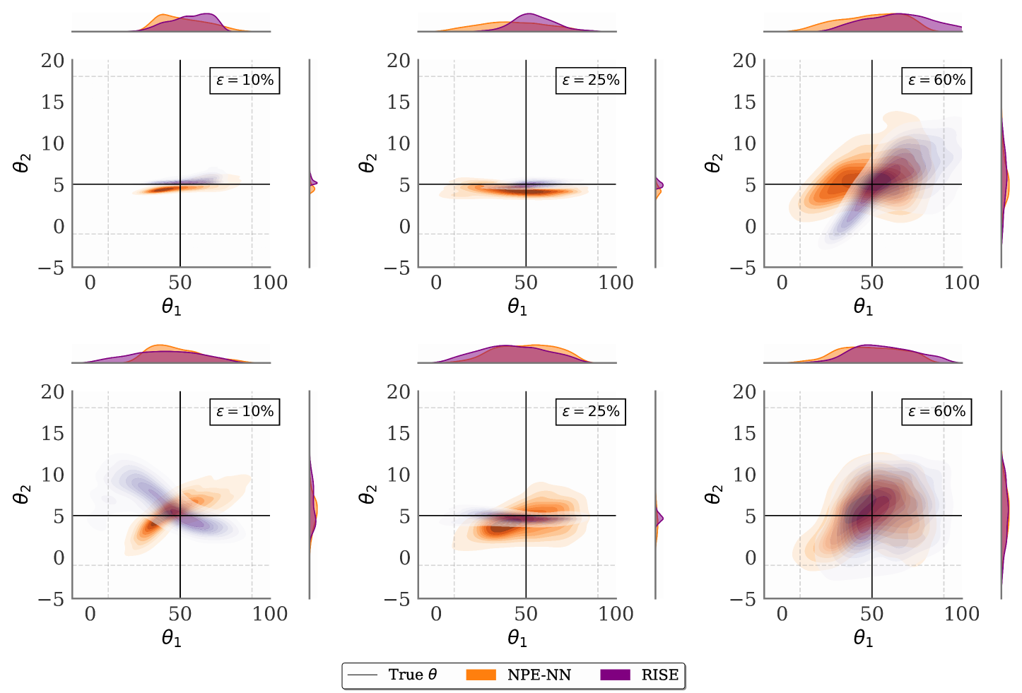
Figure 3: Posterior estimates for the Hodgkin-Huxley model under MCAR (top row) and MNAR (bottom row) with varying proportions of missing values in the data (denoted by $\varepsilon$). The posteriors obtained from RISE stay close to the true parameter (denoted by the black lines) for all values of $\varepsilon$, while those from the baseline methods move further away as $\varepsilon$ increases.

5.2 Hodgkin-Huxley model

We now apply RISE on a real-world computational neuroscience simulator (Hodgkin and Huxley, 1952), namely the Hodgkin-Huxley model, which is a popular example in the SBI literature (Lueckmann et al., 2017b; Gao et al., 2023; Gloeckler et al., 2023). The aim is to infer the posterior over two parameters given the data of dimension 1200 (see Section˜A.4.1 for the model description).

We set uniform priors and perform inference under different values of $\varepsilon$ and missingness assumptions, similar to Section˜5.1. Figure˜3 shows that RISE’s posteriors are robust to increasing proportions of missing values as they stay around the true parameter value as compared to NPE-NN. We also evaluate the expected coverage of the posterior in Section˜B.2, which demonstrates that RISE produces conservative posterior approximations and achieves better calibration than NPE-NN.

5.3 Generalizing across unknown levels of missingness

Next, we test the generalization capability of our method to unknown levels of missing values. We perform meta-learning over different proportions of missing values ${\varepsilon}$ in the dataset (termed RISE-Meta). For training RISE-Meta, we take the distribution of $p({\varepsilon})$ to be an equiprobable discrete distribution on the set $\{10\%,25\%,60\%\}$. We also train NPE-NN with a missingness degree of $60\%$ as a baseline. We evaluate all the methods over 100 samples of varying missingness proportion $\varepsilon\sim\mathcal{U}([0,1])$. Figure˜4 shows the MMD results on GLM, GLU, Ricker and OUP tasks. We observe that RISE-Meta achieves the lowest MMD values for both the tasks, thus demonstrating its ability to better generalize to unknown levels of missing values in the data.

5.4 Ablation studies

Imputation performance on real-world datasets.

We now look at how the neural process-based imputation model in RISE performs on real-world datasets. The

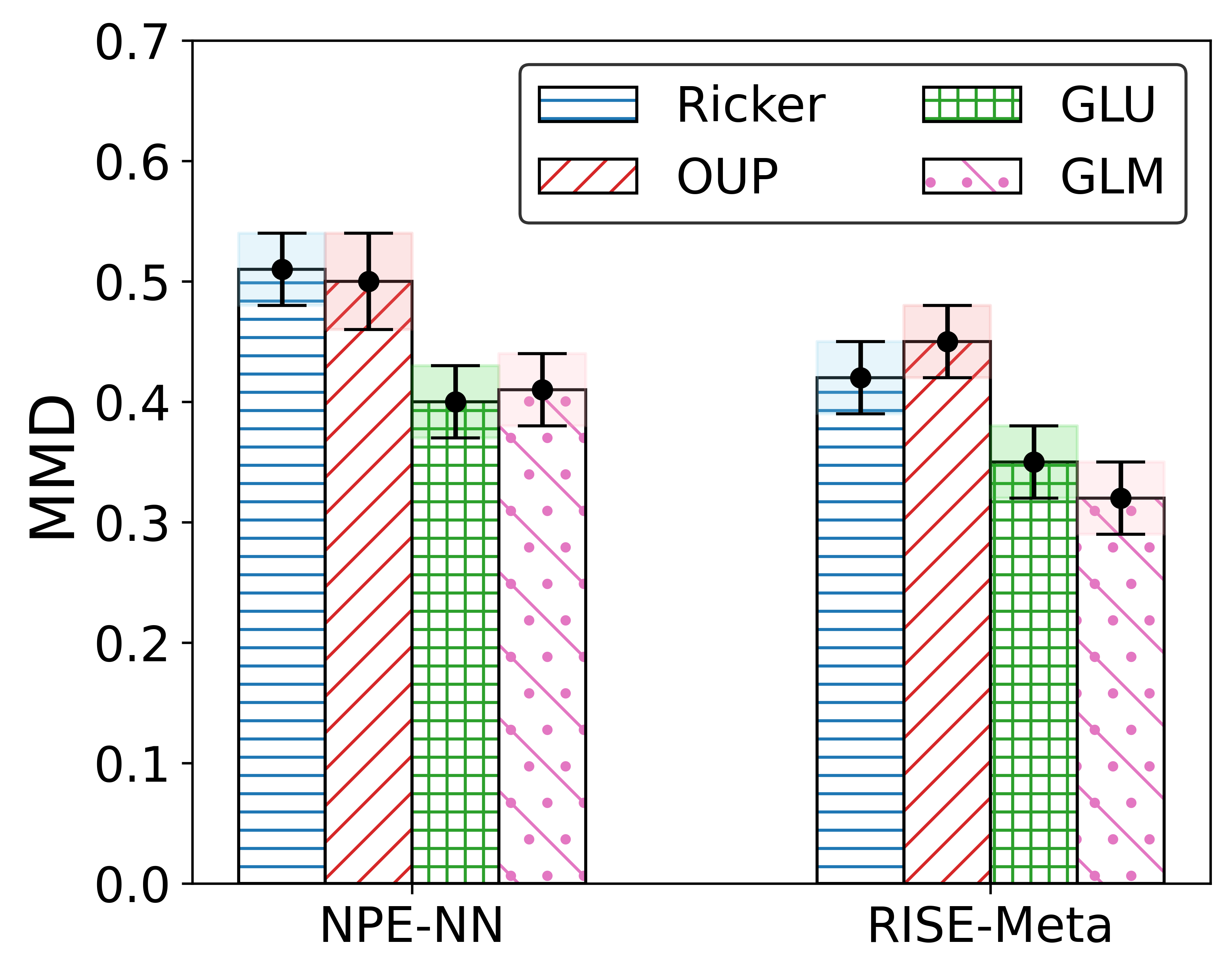
Figure 4: Generalizing over missingness.

task is to predict and impute bioactivity data on Adrenergic receptor assays (Whitehead et al., 2019) and Kinase assays (Martin et al., 2017) from the field of drug discovery. The Kinase test data consists of outliers, unlike the training data, which makes imputation challenging. We can therefore use such data to assess the generalization capabilities of RISE. We compare the RISE imputation method to other methods from this field such as QSAR (Cherkasov et al., 2014), Conduit (Whitehead et al., 2019), and Collective Matrix Factorization (CMF) (Singh and Gordon, 2008). We also include a standard deep neural network (DNN) and a vanilla neural process as baselines. Table 2 (left) reports the coefficient of determination $R^{2}$ (Wright, 1921) between the true and the predicted assays. We observe that RISE achieves state-of-the-art results in these tasks, demonstrating the efficacy of the neural processes-based imputation model.

Table 2: Ablation studies. (left) $R^{2}$ scores ($\uparrow$) on the bioactivity datasets. (right) RMSE ($\downarrow$) across different proportions of missingness ($\varepsilon$) for comparing the effect of joint versus separate learning.

Method	Adrenergic	Kinase
QSAR	(N/A)	-0.19 $\pm$ 0.01
CMF	0.59 $\pm$ 0.02	-0.11 $\pm$ 0.01
DNN	0.60 $\pm$ 0.05	0.11 $\pm$ 0.01
NP	0.61 $\pm$ 0.03	0.17 $\pm$ 0.04
Conduilt	0.62 $\pm$ 0.04	0.22 $\pm$ 0.03
CNP	0.65 $\pm$ 0.04	0.24 $\pm$ 0.02
RISE	0.67 $\pm$ 0.03	0.26 $\pm$ 0.03

Missigness ($\epsilon$)	Method	GLM	GLU
$10\%$	NPE-RF-Sep	0.69 $\pm$0.03	0.44 $\pm$0.02
	RISE-Sep	0.67 $\pm$0.03	0.43 $\pm$0.02
	RISE	0.65 $\pm$0.04	0.41$\pm$0.01
$25\%$	NPE-RF-Sep	1.02 $\pm$0.05	0.48 $\pm$0.02
	RISE-Sep	0.99 $\pm$0.03	0.45 $\pm$0.02
	RISE	0.93 $\pm$0.06	0.43 $\pm$0.02
$60\%$	NPE-RF-Sep	1.34 $\pm$0.10	0.64 $\pm$0.02
	RISE-Sep	1.31 $\pm$0.03	0.58 $\pm$0.03
	RISE	1.27 $\pm$0.01	0.56 $\pm$0.03

Joint vs separate learning.

This experiment involves investigating the impact of training the imputation and the inference model in RISE jointly (as we proposed) versus separately (termed RISE-Sep). We also include another baseline termed NPE-RF-Sep where a random forest (RF) model is first used for imputation, followed by NPE. Table 2 (right) reports the RMSE values on GLM and GLU tasks for different missingness proportion $\varepsilon$. We observe that training the imputation and inference networks jointly yields improvement in performance over training them separately.

We report the results from additional ablation studies for runtime comparisons, flow architecture, and simulation budget in Appendix˜C.

6 Conclusion and Limitations

We analyzed the problem of performing SBI under missing data and showed that inaccurately imputing the missing values may lead to bias in the resulting posterior distributions. We then proposed RISE as a method that aims to reduce this bias under different notions of the underlying missingness mechanism. RISE combines the inference network of NPE with an imputation model based on neural processes (NPs) to achieve robustness to missing data whilst being amortized. Additionally, RISE can be trained in a meta-learning manner over the proportion of missing values in the data, thus allowing for amortization across datasets with varying levels of missingness. While RISE offers substantial advantages, there are limitations to address. RISE inherits the issues of NPE and may yield posteriors that are not well-calibrated (see, e.g., Hermans et al. (2022)). Moreover, the normality assumption in NPs may exhibit limited expressivity in practice when learning complex imputation distributions.

Appendix A Appendix

Section˜A.1 discusses the aspect of handling multiple observations and model misspecfication in the context of RISE . In Section˜A.2, we present the proofs for Proposition˜1 and Proposition˜2. Section˜A.3 provides a background on neural processes, and Section˜A.4 presents the implementation details for the experiments of Section˜5. Appendix˜B contains additional metrics, coverage plots and visulaizations. Appendix˜C reports the results from additional ablation studies.

A.1 Discussion

Handling multiple observations.

Although so far we have focused on the single observation case where we have one data vector $\mathbf{x}$ for each $\theta$, RISE can straightforwardly be extended to the multiple observations case where we obtain $\mathbf{x}^{(1:m)}=(\mathbf{x}_{1},\dots,\mathbf{x}_{m})$ for each $\theta$. Then, $\mathbf{x}^{(1:m)}=(\mathbf{x}^{(1:m)}_{\text{obs}},\mathbf{x}^{(1:m)}_{\text{mis}})$, and the objective for RISE becomes

$$\operatorname*{arg\,min}_{\phi,\varphi,\kappa}-\,\mathbb{E}_{(\mathbf{x}^{(1:m)}_{\text{obs}},\theta)\sim p_{\text{true}}}\mathbb{E}_{\mathbf{x}^{(1:m)}_{\text{mis}}\sim\prod_{i=1}^{m}p(\mathbf{x}^{(i)}_{\text{mis}}\mid\mathbf{x}^{(i)}_{\text{obs}})}\left[\dfrac{1}{m}\sum_{i=1}^{m}\log\underbrace{\hat{p}_{\varphi}(\mathbf{x}^{(i)}_{\text{mis}}\mid\mathbf{x}^{(i)}_{\text{obs}})}_{\textbf{(imputation)}}+\log\underbrace{q_{\phi}(\theta\mid\eta_{\kappa}(\mathbf{x}^{1:m}_{\text{obs}},\mathbf{x}^{1:m}_{\text{mis}}))}_{\textbf{(inference)}}\right].$$

Note that we can summarize the data using the network $\eta_{\kappa}$ (for instance, a deep set [Zaheer et al., 2017]) before passing the data into the inference network, which is standard practice when using NPE with multiple observations [Chan et al., 2018]. Alternatively, one could use recent extensions based on score estimation [Geffner et al., 2023, Linhart et al., 2024] as well.

Handling model misspecification.

We conjecture that replacing the inference network in RISE from the usual NPE to a robust variant such as the method of Ward et al. [2022] or Huang et al. [2023] would help in addressing model misspecification issues. It would be an interesting avenue for future research to see how to train these robust NPE methods jointly with the imputation network of RISE, and how effective such an approach is. One way is to assume a certain error model over the observed data $\mathbf{x}$, corrupt the data to $\tilde{\mathbf{x}}$ by adding a Gaussian noise, and infer the correct $\theta$ via the inference network. This can be formulated as

$$\mathrm{argmin}_{\phi,\varphi}-\mathbb{E}_{(\mathbf{x}_{\text{obs}},\theta)\sim p(\mathbf{x}_{\text{obs}},\theta),\tilde{\mathbf{x}}_{\text{obs}}\sim\mathcal{N}(\mathbf{x}_{\text{obs}},\sigma^{2}),{\mathbf{\tilde{x}}}_{\text{mis}}\sim p_{\text{true}}(\mathbf{\tilde{x}}_{\text{mis}}\mid\mathbf{\tilde{x}}_{\text{obs}},\theta)}\left[\log\hat{p}_{\varphi}(\mathbf{\tilde{x}}_{\text{mis}}\mid\mathbf{\tilde{x}}_{\text{obs}})+\log q_{\phi}(\theta\mid\mathbf{\tilde{x}}_{\text{obs}},{\mathbf{\tilde{x}}}_{\text{mis}})\right].$$ (9)

Moreover, our method can also be readily extended to incorporate prior mis-specification:

$$\mathrm{argmin}_{\phi,\varphi}-\mathbb{E}_{(\mathbf{x}_{\text{obs}},\theta)\sim p(\mathbf{x}_{\text{obs}},\theta),\tilde{\theta}\sim\mathcal{N}(\theta,\sigma^{2}),{\mathbf{\tilde{x}}}_{\text{mis}}\sim p_{\text{true}}(\mathbf{\tilde{x}}_{\text{mis}}\mid\mathbf{\tilde{x}}_{\text{obs}},\tilde{\theta})}\left[\log\hat{p}_{\varphi}(\mathbf{\tilde{x}}_{\text{mis}}\mid\mathbf{\tilde{x}}_{\text{obs}})+\log q_{\phi}(\theta\mid\mathbf{\tilde{x}}_{\text{obs}},{\mathbf{\tilde{x}}}_{\text{mis}})\right].$$ (10)

A.2 Proofs

A.2.1 Proof for Proposition˜1

Proof.

Using Equation˜2 and Equation˜3, we note that

$$\mathbb{E}_{\theta\sim p_{\text{SBI}}(\theta\,|\,\mathbf{x}_{\text{obs}})}[\theta]-\mathbb{E}_{\theta\sim\hat{p}_{\text{SBI}}(\theta\,|\,\mathbf{x}_{\text{obs}})}[\theta]$$

$$=\int\theta p_{\text{SBI}}(\theta\,|\,\mathbf{x}_{\text{obs}})d\theta-\int\theta\hat{p}_{\text{SBI}}(\theta\,|\,\mathbf{x}_{\text{obs}})d\theta$$

$$=\int\theta\left[p_{\text{SBI}}(\theta\,|\,\mathbf{x}_{\text{obs}})-\hat{p}_{\text{SBI}}(\theta\,|\,\mathbf{x}_{\text{obs}})\right]d\theta$$

$$=\int\theta\left[\int p_{\text{SBI}}(\theta\,|\,\mathbf{x}_{\text{obs}},\mathbf{x}_{\text{mis}})p_{\text{true}}(\mathbf{x}_{\text{mis}}\,|\,\mathbf{x}_{\text{obs}})d\mathbf{x}_{\text{mis}}-\int p_{\text{SBI}}(\theta\,|\,\mathbf{x}_{\text{obs}},\mathbf{x}_{\text{mis}})\hat{p}(\mathbf{x}_{\text{mis}}\,|\,\mathbf{x}_{\text{obs}})d\mathbf{x}_{\text{mis}}\right]d\theta$$

$$=\int\theta\int p_{\text{SBI}}(\theta\,|\,\mathbf{x}_{\text{obs}},\mathbf{x}_{\text{mis}})\left[p_{\text{true}}(\mathbf{x}_{\text{mis}}\,|\,\mathbf{x}_{\text{obs}})-\hat{p}(\mathbf{x}_{\text{mis}}\,|\,\mathbf{x}_{\text{obs}})\right]d\mathbf{x}_{\text{mis}}d\theta~.$$

Thus to ensure that the bias is zero, we require that $\hat{p}(\mathbf{x}_{\text{mis}}\,|\,\mathbf{x}_{\text{obs}})$ be aligned with $p_{\text{true}}(\mathbf{x}_{\text{mis}}\,|\,\mathbf{x}_{\text{obs}})$. ∎

A.2.2 Proof for Proposition˜2

Proof.

Recall our optimization problem from Equation˜5:

$$\operatorname*{arg\,min}_{\psi}\,\mathbb{E}_{\mathbf{x}_{\text{obs}}\sim p_{\text{true}}}\,\text{KL}[p_{\text{true}}(\theta\mid\mathbf{x}_{\text{obs}})\mid\mid r_{\psi}(\theta\mid\mathbf{x}_{\text{obs}})]~.$$

Expanding the KL term, we note that the above is equivalent to

$$\operatorname*{arg\,min}_{\psi}\,\mathbb{E}_{\mathbf{x}_{\text{obs}}\sim p_{\text{true}}}\mathbb{E}_{\theta\sim p_{\text{true}}(\theta\mid\mathbf{x}_{\text{obs}})}\log\left(\dfrac{p_{\text{true}}(\theta\mid\mathbf{x}_{\text{obs}})}{r_{\psi}(\theta\mid\mathbf{x}_{\text{obs}})}\right)~.$$

Since $p_{\text{true}}(\theta\mid\mathbf{x}_{\text{obs}})$ does not depend on $\psi$, we immediately note that the problem is equivalent to

$$\mathrm{argmin}_{\psi}\,\mathbb{E}_{\mathbf{x}_{\text{obs}}\sim p_{\text{true}}}\,\mathbb{E}_{p_{\text{true}}(\theta\mid\mathbf{x}_{\text{obs}})}[-\log\,r_{\psi}(\theta\mid\mathbf{x}_{\text{obs}})]~$$

$$=\operatorname*{arg\,max}_{\psi}\,\mathbb{E}_{(\mathbf{x}_{\text{obs}},\theta)\sim p_{\text{true}}}\,[\log\,r_{\psi}(\theta\mid\mathbf{x}_{\text{obs}})]~.$$

We now obtain a lower bound for $\mathbb{E}_{(\mathbf{x}_{\text{obs}},\theta)\sim p_{\text{true}}}\,[\log\,r_{\psi}(\theta\mid\mathbf{x}_{\text{obs}})]$. Formally, we have

$$\mathbb{E}_{(\mathbf{x}_{\text{obs}},\theta)\sim p_{\text{true}}}[\log r_{\psi}(\theta\mid\mathbf{x}_{\text{obs}})] =\mathbb{E}_{(\mathbf{x}_{\text{obs}},\theta)\sim p_{\text{true}}}\log\int r_{\psi}(\theta,\mathbf{x}_{\text{mis}}\mid\mathbf{x}_{\text{obs}})d\mathbf{x}_{\text{mis}}$$

$$=\mathbb{E}_{(\mathbf{x}_{\text{obs}},\theta)\sim p_{\text{true}}}\log\int\frac{p(\mathbf{x}_{\text{mis}}\mid\mathbf{x}_{\text{obs}})r_{\psi}(\theta,\mathbf{x}_{\text{mis}}\mid\mathbf{x}_{\text{obs}})}{p(\mathbf{x}_{\text{mis}}\mid\mathbf{x}_{\text{obs}})}d\mathbf{x}_{\text{mis}}$$

$$\geq\mathbb{E}_{(\mathbf{x}_{\text{obs}},\theta)\sim p_{\text{true}}}\mathbb{E}_{\mathbf{x}_{\text{mis}}\sim p(\mathbf{x}_{\text{mis}}\mid\mathbf{x}_{\text{obs}})}\left[\log\frac{r_{\psi}(\theta,\mathbf{x}_{\text{mis}}\mid\mathbf{x}_{\text{obs}})}{p(\mathbf{x}_{\text{mis}}\mid\mathbf{x}_{\text{obs}})}\right]~$$

$$=\mathbb{E}_{(\mathbf{x}_{\text{obs}},\theta)\sim p_{\text{true}}}\mathbb{E}_{\mathbf{x}_{\text{mis}}\sim p(\mathbf{x}_{\text{mis}}\mid\mathbf{x}_{\text{obs}})}\left[\log\frac{r_{\psi}(\mathbf{x}_{\text{mis}}\mid\mathbf{x}_{\text{obs}})r_{\psi}(\theta\mid\mathbf{x}_{\text{obs}},\mathbf{x}_{\text{mis}})}{p(\mathbf{x}_{\text{mis}}\mid\mathbf{x}_{\text{obs}})}\right]~,$$

where we invoked the Jensen’s inequality to swap the log and the conditional expectation. Splitting parameters $\psi$ into imputation parameters $\varphi$ and inference parameters $\phi$, and denoting the corresponding imputation and inference networks by $\hat{p}_{\varphi}$ and $q_{\phi}$ respectively, we immediately get

$$\mathbb{E}_{(\mathbf{x}_{\text{obs}},\theta)\sim p_{\text{true}}}[\log r_{\phi,\varphi}(\theta\mid\mathbf{x}_{\text{obs}})]\geq\mathbb{E}_{(\mathbf{x}_{\text{obs}},\theta)\sim p_{\text{true}}}\mathbb{E}_{\mathbf{x}_{\text{mis}}\sim p(\mathbf{x}_{\text{mis}}\mid\mathbf{x}_{\text{obs}})}\left[\log\frac{\hat{p}_{\varphi}(\mathbf{x}_{\text{mis}}\mid\mathbf{x}_{\text{obs}})q_{\phi}(\theta\mid\mathbf{x}_{\text{obs}},\mathbf{x}_{\text{mis}})}{p(\mathbf{x}_{\text{mis}}\mid\mathbf{x}_{\text{obs}})}\right].$$

Thus, we obtain the following variational objective:

$$\mathrm{argmax}_{\phi,\varphi}\mathbb{E}_{(\mathbf{x}_{\text{obs}},\theta)\sim p_{\text{true}}}\mathbb{E}_{\mathbf{x}_{\text{mis}}\sim p(\mathbf{x}_{\text{mis}}\mid\mathbf{x}_{\text{obs}})}\left[\log\frac{\hat{p}_{\varphi}(\mathbf{x}_{\text{mis}}\mid\mathbf{x}_{\text{obs}})q_{\phi}(\theta\mid\mathbf{x}_{\text{obs}},\mathbf{x}_{\text{mis}})}{p(\mathbf{x}_{\text{mis}}\mid\mathbf{x}_{\text{obs}})}\right]$$

$$=\,\, \mathrm{argmax}_{\phi,\varphi}\mathbb{E}_{(\mathbf{x}_{\text{obs}},\theta)\sim p_{\text{true}}}\left(\mathbb{E}_{\mathbf{x}_{\text{mis}}\sim p(\mathbf{x}_{\text{mis}}\mid\mathbf{x}_{\text{obs}})}\left[\log\hat{p}_{\varphi}(\mathbf{x}_{\text{mis}}\mid\mathbf{x}_{\text{obs}})+\log q_{\phi}(\theta\mid\mathbf{x}_{\text{obs}},\mathbf{x}_{\text{mis}})\right]~+~\mathbb{H}(p(\mathbf{x}_{\text{mis}}\mid\mathbf{x}_{\text{obs}})\right)$$

$$=\,\, \mathrm{argmax}_{\phi,\varphi}\mathbb{E}_{(\mathbf{x}_{\text{obs}},\theta)\sim p_{\text{true}}}\mathbb{E}_{\mathbf{x}_{\text{mis}}\sim p(\mathbf{x}_{\text{mis}}\mid\mathbf{x}_{\text{obs}})}\left[\log\underbrace{\hat{p}_{\varphi}(\mathbf{x}_{\text{mis}}\mid\mathbf{x}_{\text{obs}})}_{\text{imputation}}+\log\underbrace{q_{\phi}(\theta\mid\mathbf{x}_{\text{obs}},\mathbf{x}_{\text{mis}})}_{\text{inference}}\right]~,$$

since the entropy term $\mathbb{H}(p(\mathbf{x}_{\text{mis}}\mid\mathbf{x}_{\text{obs}})$ does not depend on the optimization variables $\phi$ and $\varphi$.

∎

A.3 Neural process

Neural Process [Garnelo et al., 2018, Foong et al., 2020] models the predictive distribution over target locations $\mathbf{x}_{t}$ by, (i) constructing a learnable mapping $f_{\gamma}$ from the context set $(\mathbf{x}_{c},\mathbf{y}_{c})$ to a latent representation $\mathbf{r}$ as,

$$\mathbf{r}=f_{\gamma}(\mathbf{x}_{c},\mathbf{y}_{c})$$ (11)

and then (ii) utilizing the representation $\mathbf{r}$ to approximate the predictive distribution, given the target locations $\mathbf{x}_{t}$, via a learnable decoder $g_{\omega}$ as,

$$p(\mathbf{y}_{t}\mid\mathbf{x}_{t},\mathbf{r})=g_{\omega}(\mathbf{r},\mathbf{x}_{t})$$ (12)

where $\mathbf{x}_{c},\mathbf{x}_{t}\in\mathcal{X}\subseteq\mathbb{R}^{d_{x}}$ are the input vectors (often locations or positions) and $\mathbf{y}_{c},\mathbf{y}_{t}\in\mathcal{Y}\subseteq\mathbb{R}^{d_{y}}$ the output vectors. In practice, the predictive distribution is often assumed to factorize as a product of Gaussians:

$$p(\mathbf{y}_{t}\mid\mathbf{x}_{t},\mathbf{r})=\prod_{m=1}^{M}p(\mathbf{y}_{t,m}\mid\mathbf{x}_{t,m},\mathbf{r} )=\prod_{m=1}^{M}\mathcal{N}(\mathbf{y}_{t,m}\mid\mu_{\omega,m},\sigma^{2}_{\omega,m})$$ (13)

where $\mu_{\omega,m},\sigma_{\omega,m}=g_{\omega}(\mathbf{r},\mathbf{x}_{t,m})$. For a fixed context $(\mathbf{x}_{c},\mathbf{y}_{c})$, using Kolmogorov’s extension theorem [Oksendal, 2013], the collection of these finite dimensional distributions defines a stochastic process if these are consistent under (i) permutations of any entries of $(\mathbf{x}_{t},\mathbf{y}_{t})$ and (ii) marginalisations of any entries of $\mathbf{y}_{t}$.

A.4 Implementation Details

This section is arranged as follows:

• Section˜A.4.1: Description of SBI benchmarking simulators

• Section˜A.4.2: Prior distributions used for the SBI experiments

• Section˜A.4.3: Procedure for creating the missingness mask under MCAR and MNAR

• Section˜A.4.4: Details of the neural network settings.

A.4.1 Model descriptions

Ricker model simulates the temporal evolution of population size in ecological systems. In this model, the population size $N_{t}$ at time $t$ evolves as $N_{t+1}=N_{t}\exp(\theta_{1})\exp(N_{t}+e_{t}),t\in\{1,\ldots,T\}$. The parameter $\exp(\theta_{1})$ represents the growth rate, while $e_{t}$ denote independent and identically distributed Gaussian noise terms with zero mean and variance $\sigma_{e}^{2}$. The initial population size is set to $N_{0}=1$. Observations $x_{t}$ are modeled as Poisson random variables with rate parameter $\theta_{2}N_{t}$, such that $x_{t}\sim\mathrm{Poiss}(\theta_{2}N_{t})$. For our simulations, we fixed $\sigma_{e}^{2}=0.09$ and focused on estimating the parameter vector $\theta=[\theta_{1},\theta_{2}]^{\top}$. The prior distribution is set as a uniform distribution $\mathcal{U}([2,8]\times[0,20])$. We simulated the process for $T=100$ time steps to generate sufficient data for inference, and considered a simulation budget of 1000 to create the dataset.

Ornstein-Uhlenbeck process (OUP) is a stochastic differential equation model widely used in financial mathematics and evolutionary biology. The OU process $x_{t}$ is defined as,

$$x_{t+1} =x_{t}+\Delta x_{t},\quad t\in\{1,\ldots,T\}$$ (14)

$$\Delta x_{t} =\theta_{1}[\exp(\theta_{2})-x_{t}]\Delta t+0.5w$$ (15)

where $T=25$, $\Delta t=0.2$, $x_{0}=10$, and $w\sim\mathcal{N}(0,\Delta t)$.

Generalized Linear Model (GLM). A $10$ parameter Generalized Linear Model (GLM) with Bernoulli observations.

Gaussian Linear Uniform (GLU). A $10$ dimensional Gaussian model, where data points are simulated as $x\sim\mathcal{N}(x\mid\theta,\Sigma)$. The parameter $\theta$ is the mean, and the covariance $\Sigma=0.1\mathbb{I}$ is fixed, with a uniform prior ($\theta\in\mathcal{U}([-1,1]^{10})$). We refer to Lueckmann et al. [2021], Tejero-Cantero et al. [2020] for further details on these SBI tasks.

Hodgkin Huxley Model. Hodgkin Huxley Model is a real-world computational neuroscience simulator. It describes the intricate dynamics of the generation and propagation of action potentials along neuronal membranes with the capture of the time course of membrane voltage by modeling the behavior of ion channels, particularly sodium and potassium, as well as leak currents. It consists of two parameters: $\theta_{1}\equiv\bar{g}_{\text{Na}}$, and $\theta_{2}\equiv\bar{g}_{\text{K}}$, which describe the density of Na and K specifically. The dynamics are parameterized as a set of differential equations,

$$C_{m}\frac{dV}{dt} =g_{1}(E-V)+\theta_{1}m^{3}h(E_{\text{Na}}-V)+\theta_{2}n^{4}h(E_{\text{K}}-V)+\bar{g}_{\text{M}}p(E_{\text{M}}-V)+I_{\text{inj}}+\sigma\eta(t)$$

$$\frac{dq}{dt} =\frac{q_{\infty}(V)-q}{\tau_{q}(V)},~~q\in\{m,h,n,p\}$$

Here, $V$ represents the membrane potential, $C_{m}$ the membrane capacitance, $g_{1}$ is the leak conductance, $E_{1}$ is the membrane reverse potential, $\theta_{1},\theta_{2}$ are the densities of Na and K channel, $\bar{g}_{\text{M}}$ is the density for M channel, $E_{\text{Na,K,M}}$ denotes the reversal potential, and $\sigma\eta(t)$ is the intrinsic neural noise. The right hand side of the voltage dynamics is composed of a leak current, a voltage-dependent $\text{Na}^{+}$, a delayed rectifier $\text{K}^{+}$, a slow voltage-dependent $\text{K}^{+}$ current responsible for spike-frequency adaptation, and an injected current $I_{\text{inj}}$. Channel gating variables $q$ have dynamics fully characterized by the neuron membrane potential $V$, given the respective steady-state $q_{\infty}(V)$ and time constant $\tau_{q}(V)$. For more details, see Pospischil et al. [2008].

A.4.2 Prior distributions

We utilize the following prior distributions for our experiment tasks:

• Ricker: Uniform distribution $\mathcal{U}([2,8]\times[0,20])$

• OUP: Uniform prior $\mathcal{U}([0,2]\times[-2,2])$

• Hodgkin-Huxley: Uniform distribution $\mathcal{U}([10^{-4},-0.5]\times[15.0,100.0])$

• GLU: Uniform distribution $\mathcal{U}([-1,1]^{10})$

• GLM: A multivariate normal $\mathcal{N}(0,(\textbf{F}^{\top}\textbf{F})^{-1})$ computed as follows,

  $$\textbf{F}_{i,i-2}=1,\textbf{F}_{i,i-1}=-2,\textbf{F}_{i,i}=1+\sqrt{\frac{i-1}{9}},\textbf{F}_{i,j}=0~\text{otherwise},1\leq i,j\leq 9$$ (16)

A.4.3 Creating the missingness mask

MCAR.

We adopted random masking to simulate the MCAR scenario. For a given missingness degree $\varepsilon$, we randomly mask out $\varepsilon\%$ of the data sample.

MNAR.

We employed the self-masking or self-censoring approach as outlined by Ipsen et al. [2020]. For a given data sample $\mathbf{x}\in\mathbb{R}^{d}$, and following Sinelnikov et al. [2024], Ong et al. [2024], the probability of a particular data-point to be missing depends on its value. Specifically, we sample the mask $s_{i}$ for $i^{th}$ value for data sample as,

$$s_{i}\sim\mathrm{Bern}(p_{i}),\quad p_{i}={\varepsilon}\cdot\frac{x_{i}}{\max_{d}(\mathbf{x})}$$ (17)

where $0\leq i\leq d$, $\max_{d}(\mathbf{x})$ represents the maximum value in the data sample and $p_{i}$ is the masking probability for data-point $x_{i}$ which is computed using the proportion of missing values $\varepsilon$.

A.4.4 Network Parametrization

Summary Networks.

For the Ricker and Huxley model, the summary network is composed of 1D convolutional layers, whereas for the OUP, it is a combination of bidirectional long short-term memory (LSTM) recurrent modules and 1D convolutional layers. The dimension of the statistic space is set to four for both the models. We do not use summary networks for GLM and GLU.

Imputation Model.

The parameters for the neural process-based imputation model used in RISE are given in Table˜3 and Table˜4.

Table 3: Default hyperparameters for imputation model $\hat{p}_{\varphi}$ for Ricker, OUP and Huxley model.

Module	Hyperparameter	Meaning	Value
Encoder	CNN blocks	Number of CNN layers	1
	Hidden dimension	Number of output channels of each CNN layer	64
	Kernel size	Kernel size of each convolution layer	9
	Stride	Stride of each convolution layer	1
	Padding	Padding size of each convolution layer	4
Latent	CNN blocks	Number of CNN layers	2
	Hidden dimension	Number of output channels of each CNN layer	32
	Kernel size	Kernel size of each convolution layer	3
	Stride	Stride of each convolution layer	1
	Padding	Padding size of each convolution layer	1
Decoder	CNN blocks	Number of CNN layers	[6,1]
	Hidden dimension	Number of output channels of each CNN layer	[32,2]
	Kernel size	Kernel size of each convolution layer	5
	Stride	Stride of each convolution layer	1
	Padding	Padding size of each convolution layer	2

Table 4: Default hyperparameters for imputation model $\hat{p}_{\varphi}$ for GLM and GLU.

Module	Hyperparameter	Meaning	Value
Encoder	MLP blocks	Number of MLP layers	[1,1]
	Hidden dimension	Number of output channels of each MLP layer	[32,64]
Latent	MLP blocks	Number of MLP layers	2
	Hidden dimension	Number of output channels of each MLP layer	32
Decoder	MLP blocks	Number of MLP layers	[6,1]
	Hidden dimension	Number of output channels of each MLP layer	[32,10]

Inference model.

Our inference model implementations are based on publicly available code from the sbi library https://github.com/mackelab/sbi. We use the NPE-C model [Greenberg et al., 2019] with Masked Autoregressive Flow (MAF) [Papamakarios et al., 2017] as the backbone inference network, and adopt the default configuration with 20 hidden units and 5 transforms for MAF. Throughout our experiments, we maintained a consistent batch size of 50 and a fixed learning rate of $5\times 10^{-4}$.

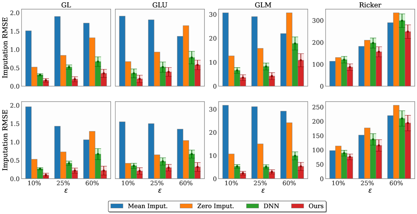
Figure 5: Imputation RMSE for MCAR (top) and MNAR (bottom) over various synthetic datasets. Here GL refers to a 10 dimension Gaussian linear model, see Lueckmann et al. [2021] for details.

Appendix B Additional Results

Figure˜5 shows how accurate our proposed method is in imputing the values of missing data simulated from the SBI benchmark models compared to the baselines. The performance is measured in terms of RMSE of the imputed values. Our method (denoted in red) performs the best in imputing the missing values (which eventually helps in improving the estimation of the posterior distribution).

B.1 MMD

In Table˜5, we report the MMD values for the experiment on SBI benchmark simulators presented in Section˜5.1. Similar to the NLPP and C2ST results of Table˜1, we observe that RISE yields lowest MMD for almost all the cases, especially for Ricker and OUP where RISE beats the baselines comprehensively.

Table 5: MMD under MCAR and MNAR scenarios, with missing value proportion $\varepsilon$. RISE demonstrates superior posterior estimation performance. For MNAR scenarios, the proportion of missing values averages below $\varepsilon$ due to self-censoring (details in Section˜A.4.3). Note that Simformer results are unavailable for Ricker and OUP due to the lack of official implementation.

	Dataset	$\epsilon$	MCAR					MNAR
			NPE-NN	Wang et al.	Simformer	RISE		NPE-NN	Wang et al.	Simformer	RISE
MMD	GLU	$10\%$	$0.21\pm 0.02$	$0.20\pm 0.03$	$0.20\pm 0.01$	$\mathbf{0.18}\pm 0.01$		$0.25\pm 0.03$	$0.23\pm 0.02$	$0.18\pm 0.01$	$\mathbf{0.16}\pm 0.01$
		$25\%$	$0.27\pm 0.02$	$0.27\pm 0.01$	$0.27\pm 0.01$	$\mathbf{0.26}\pm 0.01$		$0.29\pm 0.02$	$0.26\pm 0.02$	$0.25\pm 0.01$	$\mathbf{0.22}\pm 0.02$
		$60\%$	$0.40\pm 0.04$	$0.36\pm 0.02$	$0.39\pm 0.03$	$\mathbf{0.33}\pm 0.03$		$0.33\pm 0.02$	$0.31\pm 0.02$	$0.32\pm 0.02$	$\mathbf{0.27}\pm 0.02$
	GLM	$10\%$	$0.15\pm 0.01$	$0.15\pm 0.02$	$0.17\pm 0.01$	$\mathbf{0.12}\pm 0.01$		$0.16\pm 0.01$	$0.14\pm 0.02$	$0.16\pm 0.01$	$\mathbf{0.13}\pm 0.01$
		$25\%$	$0.37\pm 0.02$	$0.30\pm 0.02$	$0.31\pm 0.03$	$\mathbf{0.27}\pm 0.03$		$0.18\pm 0.02$	$0.22\pm 0.02$	$0.25\pm 0.03$	$\mathbf{0.17}\pm 0.01$
		$60\%$	$0.50\pm 0.04$	$0.44\pm 0.02$	$0.52\pm 0.03$	$\mathbf{0.38}\pm 0.05$		$0.62\pm 0.04$	$0.53\pm 0.02$	$0.50\pm 0.03$	$\mathbf{0.47}\pm 0.02$
	Ricker	$10\%$	$0.45\pm 0.01$	$0.38\pm 0.02$	-	$\mathbf{0.31}\pm 0.01$		$0.49\pm 0.01$	$0.32\pm 0.02$	-	$\mathbf{0.27}\pm 0.02$
		$25\%$	$0.47\pm 0.02$	$0.39\pm 0.02$	-	$\mathbf{0.35}\pm 0.02$		$0.49\pm 0.02$	$0.41\pm 0.02$	-	$\mathbf{0.36}\pm 0.03$
		$60\%$	$0.51\pm 0.02$	$0.43\pm 0.02$	-	$\mathbf{0.37}\pm 0.01$		$0.57\pm 0.01$	$0.46\pm 0.02$	-	$\mathbf{0.41}\pm 0.05$
	OUP	$10\%$	$0.35\pm 0.02$	$0.31\pm 0.02$	-	$\mathbf{0.29}\pm 0.02$		$0.42\pm 0.03$	$0.41\pm 0.02$	-	$\mathbf{0.38}\pm 0.03$
		$25\%$	$0.36\pm 0.02$	$0.33\pm 0.02$	-	$\mathbf{0.30}\pm 0.02$		$0.43\pm 0.02$	$0.41\pm 0.02$	-	$\mathbf{0.38}\pm 0.02$
		$60\%$	$0.39\pm 0.03$	$0.37\pm 0.02$	-	$\mathbf{0.35}\pm 0.02$		$0.44\pm 0.03$	$0.41\pm 0.02$	-	$\mathbf{0.39}\pm 0.02$

B.2 Coverage Plots

We compute the expected coverage [Hermans et al., 2022] of our method on various confidence levels. Figure˜6 shows the expected coverage for the HH task and GLU at various levels of missingness. We observe that RISE is able to produce conservative posterior approximations, and is better calibrated than NPE-NN.

Figure 6: Expected coverage of RISE and NPE-NN for HH (top) and GLU (bottom) task over various level of missingness. The estimator becomes more conservative with increase in missingness due to the lack of information to estimate posterior and imputation distribution.

B.3 Additional visualizations

The fig.˜7 offers further insight into the posterior bias illustrated in fig.˜1, specifically from the perspective of learned statistics. Our observations indicate that statistics for augmented datasets deviate from the fully observed statistic value, consequently causing a shift in the corresponding NPE posterior away from the true parameter value.

Figure 7: Shifting Statistics. The corresponding learned statistics for fully observed and augmented datasets as described in fig.˜1. Observe that the statistics for augmented datasets shift away from the fully observed statistic value, thereby leading to a shift in the corresponding NPE posterior away from the true parameter value. Note that as we re-train the method for each missingness level, the three statistics plots should not be compared with each other.

Appendix C Additional Ablation Studies

Performance as function of simulation budget.

We conduct a study to quantify RISE’s performance as a function of the simulation budget on GLU and GLM dataset. Table˜7 shows C2ST and MMD for different simulation budgets for RISE, for $10\%$ missingness level. As the budget increases, the performance improves. We also visualize the posterior obtained for different simulation budgets for Ricker and OUP in LABEL:fig:ricker_plot.

Runtime comparison.

We perform an ablation study to compare the computational complexity of RISE to that of standard NPE. Table˜7 describes the time (in seconds) per epoch to train different models on a single V100 GPU. We observe that there is a minimal increase in runtime due to the inclusion of the imputation model. The training time remains the same with respect to missingness levels over a certain data dimensionality.

Flow architecture.

Our final experiment involves comparing RISE’s performance for different flow architectures. We utilize neural spline flow [Durkan et al., 2019] and masked autoregressive flow as competing architectures and evaluate on the GLM model under $10\%$ missigness. Table˜6 shows that both NSF and MAF yield similar results.

Table 6: Ablation on flow architectures (left) and meta learning the missingness (right).

Method	C2ST	RMSE	MMD
RISE-MAF	0.80	0.65	0.12
RISE-NSF	0.80	0.67	0.11

Method	Ricker		OUP
	RMSE	MMD	RMSE	MMD
NPE-NN	1.97	0.51	1.32	0.50
RISE-Meta	1.52	0.42	0.89	0.45

Table 7: Runtime comparisons (left) and Simulation budget comparisons (right).

Method	GLM	GLU
NPE	0.12	0.10
RISE	0.18	0.16

Budget	GLU		GLM
	C2ST	MMD	C2ST	MMD
1000	0.83	0.18	0.80	0.12
10000	0.78	0.15	0.75	0.10

References

- Bharti et al. (2022a) Ayush Bharti, Francois-Xavier Briol, and Troels Pedersen. A general method for calibrating stochastic radio channel models with kernels. IEEE Transactions on Antennas and Propagation, 70(6):3986–4001, 2022a. doi: 10.1109/tap.2021.3083761.
- Bharti et al. (2022b) Ayush Bharti, Louis Filstroff, and Samuel Kaski. Approximate Bayesian computation with domain expert in the loop. In International Conference on Machine Learning, volume 162, pages 1893–1905, 2022b.
- Briol et al. (2019) F-X. Briol, A. Barp, A. B. Duncan, and M. Girolami. Statistical inference for generative models with maximum mean discrepancy. arXiv:1906.05944, 2019.
- Casale et al. (2018) Francesco Paolo Casale, Adrian Dalca, Luca Saglietti, Jennifer Listgarten, and Nicolo Fusi. Gaussian process prior variational autoencoders. Advances in neural information processing systems, 31, 2018.
- Chan et al. (2018) Jeffrey Chan, Valerio Perrone, Jeffrey Spence, Paul Jenkins, Sara Mathieson, and Yun Song. A likelihood-free inference framework for population genetic data using exchangeable neural networks. Advances in neural information processing systems, 31, 2018.
- Chen et al. (2021) Yanzhi Chen, Dinghuai Zhang, Michael U. Gutmann, Aaron Courville, and Zhanxing Zhu. Neural approximate sufficient statistics for implicit models. In International Conference on Learning Representations, 2021.
- Cherkasov et al. (2014) Artem Cherkasov, Eugene N Muratov, Denis Fourches, Alexandre Varnek, Igor I Baskin, Mark Cronin, John Dearden, Paola Gramatica, Yvonne C Martin, Roberto Todeschini, et al. Qsar modeling: where have you been? where are you going to? Journal of medicinal chemistry, 57(12):4977–5010, 2014.
- Collier et al. (2020) Mark Collier, Alfredo Nazabal, and Christopher KI Williams. Vaes in the presence of missing data. arXiv preprint arXiv:2006.05301, 2020.
- Cranmer et al. (2020) Kyle Cranmer, Johann Brehmer, and Gilles Louppe. The frontier of simulation-based inference. Proceedings of the National Academy of Sciences, 117(48):30055–30062, 2020.
- Dax et al. (2021) Maximilian Dax, Stephen R. Green, Jonathan Gair, Jakob H. Macke, Alessandra Buonanno, and Bernhard Schölkopf. Real-time gravitational wave science with neural posterior estimation. Physical Review Letters, 127(24):241103, December 2021. ISSN 1079-7114. doi: 10.1103/physrevlett.127.241103.
- Dellaporta et al. (2022) Charita Dellaporta, Jeremias Knoblauch, Theodoros Damoulas, and Francois-Xavier Briol. Robust bayesian inference for simulator-based models via the mmd posterior bootstrap. In International Conference on Artificial Intelligence and Statistics, volume 151, pages 943–970, 2022.
- Dubois et al. (2020) Yann Dubois, Jonathan Gordon, and Andrew YK Foong. Neural process family. http://yanndubs.github.io/Neural-Process-Family/, September 2020.
- Durkan et al. (2019) Conor Durkan, Artur Bekasov, Iain Murray, and George Papamakarios. Neural spline flows. Advances in neural information processing systems, 32, 2019.
- Foong et al. (2020) Andrew Foong, Wessel Bruinsma, Jonathan Gordon, Yann Dubois, James Requeima, and Richard Turner. Meta-learning stationary stochastic process prediction with convolutional neural processes. Advances in Neural Information Processing Systems, 33:8284–8295, 2020.
- Fortuin et al. (2020) Vincent Fortuin, Dmitry Baranchuk, Gunnar Ratsch, and Stephan Mandt. Gp-vae: Deep probabilistic time series imputation. In International conference on artificial intelligence and statistics, pages 1651–1661. PMLR, 2020.
- Frazier et al. (2020) David T. Frazier, Christian P. Robert, and Judith Rousseau. Model misspecification in approximate bayesian computation: consequences and diagnostics. Journal of the Royal Statistical Society: Series B (Statistical Methodology), 82(2):421–444, 2020. doi: 10.1111/rssb.12356.
- Fujisawa et al. (2021) Masahiro Fujisawa, Takeshi Teshima, Issei Sato, and Masashi Sugiyama. -abc: Outlier-robust approximate bayesian computation based on a robust divergence estimator. In International Conference on Artificial Intelligence and Statistics, volume 130, pages 1783–1791, 2021.
- Gao et al. (2023) Richard Gao, Michael Deistler, and Jakob H Macke. Generalized bayesian inference for scientific simulators via amortized cost estimation. Advances in Neural Information Processing Systems, 36, 2023.
- Garnelo et al. (2018) Marta Garnelo, Dan Rosenbaum, Christopher Maddison, Tiago Ramalho, David Saxton, Murray Shanahan, Yee Whye Teh, Danilo Rezende, and SM Ali Eslami. Conditional neural processes. In International conference on machine learning, pages 1704–1713. PMLR, 2018.
- Geffner et al. (2023) Tomas Geffner, George Papamakarios, and Andriy Mnih. Compositional score modeling for simulation-based inference. In International Conference on Machine Learning, pages 11098–11116. PMLR, 2023.
- Gelman et al. (1995) Andrew Gelman, John B Carlin, Hal S Stern, and Donald B Rubin. Bayesian data analysis. Chapman and Hall/CRC, 1995.
- Ghalebikesabi et al. (2021a) Sahra Ghalebikesabi, Rob Cornish, Chris Holmes, and Luke Kelly. Deep generative missingness pattern-set mixture models. In International conference on artificial intelligence and statistics, pages 3727–3735. PMLR, 2021a.
- Ghalebikesabi et al. (2021b) Sahra Ghalebikesabi, Rob Cornish, Luke J. Kelly, and Chris Holmes. Deep generative pattern-set mixture models for nonignorable missingness, 2021b.
- Gloeckler et al. (2023) Manuel Gloeckler, Michael Deistler, and Jakob H Macke. Adversarial robustness of amortized bayesian inference. arXiv preprint arXiv:2305.14984, 2023.
- Gloeckler et al. (2024) Manuel Gloeckler, Michael Deistler, Christian Dietrich Weilbach, Frank Wood, and Jakob H. Macke. All-in-one simulation-based inference. In Ruslan Salakhutdinov, Zico Kolter, Katherine Heller, Adrian Weller, Nuria Oliver, Jonathan Scarlett, and Felix Berkenkamp, editors, Proceedings of the 41st International Conference on Machine Learning, volume 235 of Proceedings of Machine Learning Research, pages 15735–15766. PMLR, 21–27 Jul 2024.
- Gong et al. (2021) Yu Gong, Hossein Hajimirsadeghi, Jiawei He, Thibaut Durand, and Greg Mori. Variational selective autoencoder: Learning from partially-observed heterogeneous data. In International Conference on Artificial Intelligence and Statistics, pages 2377–2385. PMLR, 2021.
- Graham et al. (2007) JW Graham, AE Olchowski, and TD Gilreath. Review: A gentle introduction to imputation of missing values. Prev. Sci, 8:206–213, 2007.
- Greenberg et al. (2019) David Greenberg, Marcel Nonnenmacher, and Jakob Macke. Automatic posterior transformation for likelihood-free inference. In International Conference on Machine Learning, pages 2404–2414. PMLR, 2019.
- Gretton et al. (2012) Arthur Gretton, Karsten M Borgwardt, Malte J Rasch, Bernhard Schölkopf, and Alexander Smola. A kernel two-sample test. The Journal of Machine Learning Research, 13(1):723–773, 2012.
- Hermans et al. (2022) Joeri Hermans, Arnaud Delaunoy, François Rozet, Antoine Wehenkel, Volodimir Begy, and Gilles Louppe. A crisis in simulation-based inference? beware, your posterior approximations can be unfaithful. Transactions on Machine Learning Research, 2022. ISSN 2835-8856. URL https://openreview.net/forum?id=LHAbHkt6Aq.
- Hodgkin and Huxley (1952) Alan L Hodgkin and Andrew F Huxley. A quantitative description of membrane current and its application to conduction and excitation in nerve. The Journal of physiology, 117(4):500, 1952.
- Huang et al. (2023) Daolang Huang, Ayush Bharti, Amauri Souza, Luigi Acerbi, and Samuel Kaski. Learning robust statistics for simulation-based inference under model misspecification. Advances in Neural Information Processing Systems, 36, 2023.
- Ipsen et al. (2020) Niels Bruun Ipsen, Pierre-Alexandre Mattei, and Jes Frellsen. not-miwae: Deep generative modelling with missing not at random data. arXiv preprint arXiv:2006.12871, 2020.
- Kasak et al. (2024) Milosz Kasak, Kamil Deja, Maja Karwowska, Monika Jakubowska, Lukasz Graczykowski, and Malgorzata Janik. Machine-learning-based particle identification with missing data. The European Physical Journal C, 84(7):691, 2024.
- Kelly et al. (2024) Ryan P. Kelly, David J Nott, David Tyler Frazier, David J Warne, and Christopher Drovandi. Misspecification-robust sequential neural likelihood for simulation-based inference. Transactions on Machine Learning Research, 2024. ISSN 2835-8856.
- Kingma (2013) Diederik P Kingma. Auto-encoding variational bayes. arXiv preprint arXiv:1312.6114, 2013.
- Kingma (2014) Diederik P Kingma. Adam: A method for stochastic optimization. arXiv preprint arXiv:1412.6980, 2014.
- Kypraios et al. (2017) Theodore Kypraios, Peter Neal, and Dennis Prangle. A tutorial introduction to bayesian inference for stochastic epidemic models using approximate bayesian computation. Mathematical Biosciences, 287:42–53, May 2017. ISSN 0025-5564. doi: 10.1016/j.mbs.2016.07.001.
- Li et al. (2019) Steven Cheng-Xian Li, Bo Jiang, and Benjamin Marlin. Misgan: Learning from incomplete data with generative adversarial networks. International Conference on Learning Representations, 2019.
- Linhart et al. (2024) Julia Linhart, Gabriel Victorino Cardoso, Alexandre Gramfort, Sylvain Le Corff, and Pedro LC Rodrigues. Diffusion posterior sampling for simulation-based inference in tall data settings. arXiv preprint arXiv:2404.07593, 2024.
- Little and Rubin (2019) Roderick JA Little and Donald B Rubin. Statistical analysis with missing data, volume 793. John Wiley & Sons, 2019.
- Lopez-Paz and Oquab (2017) David Lopez-Paz and Maxime Oquab. Revisiting classifier two-sample tests. In International Conference on Learning Representations, 2017. URL https://openreview.net/forum?id=SJkXfE5xx.
- Lueckmann et al. (2017a) Jan-Matthis Lueckmann, Pedro J Goncalves, Giacomo Bassetto, Kaan Öcal, Marcel Nonnenmacher, and Jakob H Macke. Flexible statistical inference for mechanistic models of neural dynamics. Advances in neural information processing systems, 30, 2017a.
- Lueckmann et al. (2017b) Jan-Matthis Lueckmann, Pedro J. Gonçalves, Giacomo Bassetto, Kaan Öcal, Marcel Nonnenmacher, and Jakob H. Macke. Flexible statistical inference for mechanistic models of neural dynamics. In Advances in Neural Information Processing Systems (NIPS), page 1289–1299, 2017b.
- Lueckmann et al. (2021) Jan-Matthis Lueckmann, Jan Boelts, David Greenberg, Pedro Goncalves, and Jakob Macke. Benchmarking simulation-based inference. In International conference on artificial intelligence and statistics, pages 343–351. PMLR, 2021.
- Luken et al. (2021) Kieran J Luken, Rabina Padhy, and X Rosalind Wang. Missing data imputation for galaxy redshift estimation. arXiv preprint arXiv:2111.13806, 2021.
- Luo et al. (2018) Yonghong Luo, Xiangrui Cai, Ying Zhang, Jun Xu, et al. Multivariate time series imputation with generative adversarial networks. Advances in neural information processing systems, 31, 2018.
- Ma and Zhang (2021) Chao Ma and Cheng Zhang. Identifiable generative models for missing not at random data imputation. Advances in Neural Information Processing Systems, 34:27645–27658, 2021.
- Martin et al. (2017) Eric J Martin, Valery R Polyakov, Li Tian, and Rolando C Perez. Profile-qsar 2.0: kinase virtual screening accuracy comparable to four-concentration ic50s for realistically novel compounds. Journal of chemical information and modeling, 57(8):2077–2088, 2017.
- Mattei and Frellsen (2019) Pierre-Alexandre Mattei and Jes Frellsen. Miwae: Deep generative modelling and imputation of incomplete data sets. In International Conference on Machine Learning, pages 4413–4423. PMLR, 2019.
- Muzellec et al. (2020) Boris Muzellec, Julie Josse, Claire Boyer, and Marco Cuturi. Missing data imputation using optimal transport, 2020.
- Nazabal et al. (2020) Alfredo Nazabal, Pablo M Olmos, Zoubin Ghahramani, and Isabel Valera. Handling incomplete heterogeneous data using vaes. Pattern Recognition, 107:107501, 2020.
- Oksendal (2013) Bernt Oksendal. Stochastic differential equations: an introduction with applications. Springer Science & Business Media, 2013.
- Ong et al. (2024) Priscilla Ong, Manuel Haussmann, and Harri Lahdesmaki. Learning high-dimensional mixed models via amortized variational inference. In ICML 2024 Workshop on Structured Probabilistic Inference & Generative Modeling, 2024.
- Papamakarios and Murray (2016) George Papamakarios and Iain Murray. Fast -free inference of simulation models with bayesian conditional density estimation. Advances in neural information processing systems, 29, 2016.
- Papamakarios et al. (2017) George Papamakarios, Theo Pavlakou, and Iain Murray. Masked autoregressive flow for density estimation. Advances in neural information processing systems, 30, 2017.
- Papamakarios et al. (2019) George Papamakarios, David Sterratt, and Iain Murray. Sequential neural likelihood: Fast likelihood-free inference with autoregressive flows. In The 22nd International Conference on Artificial Intelligence and Statistics, pages 837–848. PMLR, 2019.
- Papamakarios et al. (2021) George Papamakarios, Eric Nalisnick, Danilo Jimenez Rezende, Shakir Mohamed, and Balaji Lakshminarayanan. Normalizing flows for probabilistic modeling and inference. Journal of Machine Learning Research, 22(57):1–64, 2021.
- Paszke et al. (2019) Adam Paszke, Sam Gross, Francisco Massa, Adam Lerer, James Bradbury, Gregory Chanan, Trevor Killeen, Zeming Lin, Natalia Gimelshein, Luca Antiga, et al. Pytorch: An imperative style, high-performance deep learning library. Advances in neural information processing systems, 32, 2019.
- Pesonen et al. (2023) Henri Pesonen, Umberto Simola, Alvaro Köhn-Luque, Henri Vuollekoski, Xiaoran Lai, Arnoldo Frigessi, Samuel Kaski, David T Frazier, Worapree Maneesoonthorn, Gael M Martin, et al. Abc of the future. International Statistical Review, 91(2):243–268, 2023.
- Pospischil et al. (2008) Martin Pospischil, Maria Toledo-Rodriguez, Cyril Monier, Zuzanna Piwkowska, Thierry Bal, Yves Frégnac, Henry Markram, and Alain Destexhe. Minimal hodgkin–huxley type models for different classes of cortical and thalamic neurons. Biological cybernetics, 99:427–441, 2008.
- Radev et al. (2020) Stefan T. Radev, Ulf K. Mertens, Andreas Voss, Lynton Ardizzone, and Ullrich Köthe. Bayesflow: Learning complex stochastic models with invertible neural networks, 2020. URL https://arxiv.org/abs/2003.06281.
- Raghunathan et al. (2001) Trivellore E Raghunathan, James M Lepkowski, John Van Hoewyk, Peter Solenberger, et al. A multivariate technique for multiply imputing missing values using a sequence of regression models. Survey methodology, 27(1):85–96, 2001.
- Ramchandran et al. (2021) Siddharth Ramchandran, Gleb Tikhonov, Kalle Kujanpää, Miika Koskinen, and Harri Lähdesmäki. Longitudinal variational autoencoder. In International Conference on Artificial Intelligence and Statistics, pages 3898–3906. PMLR, 2021.
- Riesselman et al. (2018) Adam J. Riesselman, John B. Ingraham, and Debora S. Marks. Deep generative models of genetic variation capture the effects of mutations. Nature Methods, 15(10):816–822, September 2018. ISSN 1548-7105. doi: 10.1038/s41592-018-0138-4.
- Rubin (1976) Donald B Rubin. Inference and missing data. Biometrika, 63(3):581–592, 1976.
- Schafer and Schenker (2000) Joseph L Schafer and Nathaniel Schenker. Inference with imputed conditional means. Journal of the American Statistical Association, 95(449):144–154, 2000.
- Schmitt et al. (2023) Marvin Schmitt, Paul-Christian Bürkner, Ullrich Köthe, and Stefan T Radev. Detecting model misspecification in amortized bayesian inference with neural networks. In DAGM German Conference on Pattern Recognition, pages 541–557. Springer, 2023.
- Sinelnikov et al. (2024) Maksim Sinelnikov, Manuel Haussmann, and Harri Lähdesmäki. Latent variable model for high-dimensional point process with structured missingness. arXiv preprint arXiv:2402.05758, 2024.
- Singh and Gordon (2008) Ajit P Singh and Geoffrey J Gordon. Relational learning via collective matrix factorization. In Proceedings of the 14th ACM SIGKDD international conference on Knowledge discovery and data mining, pages 650–658, 2008.
- Sisson (2018) Scott A. Sisson. Handbook of Approximate Bayesian Computation. Chapman and Hall/CRC, 2018.
- Smieja et al. (2018) Marek Smieja, Lukasz Struski, Jacek Tabor, Bartosz Zielinski, and Przemyslaw Spurek. Processing of missing data by neural networks. Advances in neural information processing systems, 31, 2018.
- Tejero-Cantero et al. (2020) Alvaro Tejero-Cantero, Jan Boelts, Michael Deistler, Jan-Matthis Lueckmann, Conor Durkan, Pedro J. Gonçalves, David S. Greenberg, and Jakob H. Macke. sbi: A toolkit for simulation-based inference. Journal of Open Source Software, 5(52):2505, 2020. doi: 10.21105/joss.02505.
- Van Buuren and Groothuis-Oudshoorn (2011) Stef Van Buuren and Karin Groothuis-Oudshoorn. mice: Multivariate imputation by chained equations in r. Journal of statistical software, 45:1–67, 2011.
- Vo et al. (2024) Vy Vo, He Zhao, Trung Le, Edwin V Bonilla, and Dinh Phung. Optimal transport for structure learning under missing data. arXiv preprint arXiv:2402.15255, 2024.
- Wang et al. (2022) Bingjie Wang, Joel Leja, Ashley Villar, and Joshua S Speagle. Monte carlo techniques for addressing large errors and missing data in simulation-based inference. arXiv preprint arXiv:2211.03747, 2022.
- Wang et al. (2023) Bingjie Wang, Joel Leja, V Ashley Villar, and Joshua S Speagle. Sbi++: Flexible, ultra-fast likelihood-free inference customized for astronomical applications. The Astrophysical Journal Letters, 952(1):L10, 2023.
- Wang et al. (2024) Zijian Wang, Jan Hasenauer, and Yannik Schälte. Missing data in amortized simulation-based neural posterior estimation. PLOS Computational Biology, 20(6):e1012184, 2024.
- Ward et al. (2022) Daniel Ward, Patrick Cannon, Mark Beaumont, Matteo Fasiolo, and Sebastian M Schmon. Robust neural posterior estimation and statistical model criticism. In Advances in Neural Information Processing Systems, 2022.
- Whitehead et al. (2019) Thomas M Whitehead, Benedict WJ Irwin, P Hunt, Matthew D Segall, and Gareth John Conduit. Imputation of assay bioactivity data using deep learning. Journal of chemical information and modeling, 59(3):1197–1204, 2019.
- Wood (2010) Simon N. Wood. Statistical inference for noisy nonlinear ecological dynamic systems. Nature, 466(7310):1102–1104, 2010. doi: 10.1038/nature09319.
- Wright (1921) Sewall Wright. Correlation and causation. Journal of agricultural research, 20(7):557, 1921.
- Yoon et al. (2018) Jinsung Yoon, James Jordon, and Mihaela Schaar. Gain: Missing data imputation using generative adversarial nets. In International Conference on Machine Learning, pages 5689–5698. PMLR, 2018.
- Yoon and Sull (2020) Seongwook Yoon and Sanghoon Sull. Gamin: Generative adversarial multiple imputation network for highly missing data. In Proceedings of the IEEE/CVF conference on computer vision and pattern recognition, pages 8456–8464, 2020.
- Zaheer et al. (2017) Manzil Zaheer, Satwik Kottur, Siamak Ravanbakhsh, Barnabas Poczos, Russ R Salakhutdinov, and Alexander J Smola. Deep sets. Advances in neural information processing systems, 30, 2017.
- Zhao et al. (2023) He Zhao, Ke Sun, Amir Dezfouli, and Edwin V Bonilla. Transformed distribution matching for missing value imputation. In International Conference on Machine Learning, pages 42159–42186. PMLR, 2023.
- Zhou and Reiter (2010) Xiang Zhou and Jerome P Reiter. A note on bayesian inference after multiple imputation. The American Statistician, 64(2):159–163, 2010.