Soybean Disease Detection via Interpretable Hybrid CNN-GNN: Integrating MobileNetV2 and GraphSAGE with Cross-Modal Attention

Abstract

Soybean leaf disease detection is critical for agricultural productivity but faces challenges due to visually similar symptoms and limited interpretability in conventional methods. While Convolutional Neural Networks (CNNs) excel in spatial feature extraction, they often neglect inter-image relational dependencies, leading to misclassifications. This paper proposes an interpretable hybrid Sequential CNN-Graph Neural Network (GNN) framework that synergizes MobileNetV2 for localized feature extraction and GraphSAGE for relational modeling. The framework constructs a graph where nodes represent leaf images, with edges defined by cosine similarity-based adjacency matrices and adaptive neighborhood sampling. This design captures fine-grained lesion features and global symptom patterns, addressing inter-class similarity challenges. Cross-modal interpretability is achieved via Grad-CAM and Eigen-CAM visualizations, generating heatmaps to highlight disease-influential regions. Evaluated on a dataset of ten soybean leaf diseases, the model achieves 97.16% accuracy, surpassing standalone CNNs ($\leq$95.04%) and traditional machine learning models ($\leq$77.05%). Ablation studies validate the sequential architecture’s superiority over parallel or single-model configurations. With only 2.3 million parameters, the lightweight MobileNetV2-GraphSAGE combination ensures computational efficiency, enabling real-time deployment in resource-constrained environments. The proposed approach bridges the gap between accurate classification and practical applicability, offering a robust, interpretable tool for agricultural diagnostics while advancing CNN-GNN integration in plant pathology research.

I Introduction

Soybean (Glycine max) is one of the most significant crops globally, providing essential nutrients and oil for both human consumption and animal feed. However, various diseases often threaten its production, including soybean rust, septoria brown spot, and frog eye leaf spot. These diseases severely affect the quality and yield of soybean crops, leading to substantial economic losses for farmers. Traditional methods of disease detection, primarily based on manual inspection, are time-consuming, labor-intensive, and subjective, making them unsuitable for large-scale, automated applications.

With the advent of machine learning and deep learning, significant progress has been made in automating plant disease detection, particularly through Convolutional Neural Networks (CNNs). CNNs have demonstrated strong performance in image classification tasks by automatically learning spatial features from raw images, eliminating the need for manual feature extraction. Numerous studies have highlighted their effectiveness in soybean leaf disease classification [1, 2, 3, 4, 5, 6, 7, 8, 9]. However, most existing approaches — whether using CNNs or transfer learning techniques [10, 11] — focus on extracting features from individual images, overlooking critical relational information between images. This becomes particularly problematic when diseases present visually similar symptoms triggered by different factors, such as nutrient deficiencies, pest damage, or environmental stress, often leading to misclassifications. Moreover, these conventional models offer limited explainability, providing little insight into which leaf regions drive predictions, reducing interpretability and trust among agricultural experts.

Graph Neural Networks (GNNs) have emerged as a complementary approach capable of modeling relational dependencies between samples to address these limitations. GNNs are particularly well-suited for cases where relationships between images — such as symptom similarity or shared environmental conditions — provide valuable diagnostic cues [12, 13]. By treating images as nodes and defining edges based on pairwise similarities, GNNs aggregate information from neighboring images, enabling context-aware classification incorporating local features and global relational patterns. However, GNNs alone lack the ability to extract fine-grained spatial features directly from raw images — a key strength of CNNs. Therefore, combining CNNs and GNNs into a hybrid framework offers a synergistic advantage: CNNs capture localized spatial features within individual images, while GNNs enrich these representations with relational context across images. This hybrid approach is particularly valuable for soybean leaf disease classification, where local lesion characteristics and broader symptom similarity across fields, varieties, and conditions are essential for accurate and interpretable diagnosis.

To address these gaps, we propose an interpretable hybrid Sequential CNN-GNN architecture that sequentially combines MobileNetV2 for efficient spatial feature extraction and Graph Sample and Aggregation (GraphSAGE), a GNN architecture, for relational dependency modeling between soybean leaf images. By constructing a similarity graph where nodes represent leaf images and edges encode pairwise feature similarity, GraphSage [14] aggregates information from neighboring nodes, enriching the feature representations with relational context. This fusion of local spatial learning and global relational learning enhances classification accuracy while ensuring computational efficiency, making the model suitable for real-time field deployment. Additionally, we incorporate Grad-CAM and Eigen-CAM visualizations to provide interpretable heatmaps that highlight the specific leaf regions influencing each classification decision, bridging the gap between model predictions and expert validation. To the best of our knowledge, this is the first interpretable CNN-GNN hybrid framework applied to soybean leaf disease detection, addressing critical gaps in relational modeling, model transparency, and computational efficiency in plant disease classification research.

We make the following key contributions in this work:

1. Sequential CNN-GNN Architecture: We propose a novel pipeline combining a pre-trained MobileNetV2 for local feature extraction and a GraphSAGE model for global relational reasoning, enhancing our model’s ability to capture fine-grained disease symptoms and inter-symptom dependencies.

2. Graph Construction with Node Fusion and Adaptive Sampling: We introduce a domain-specific graph construction where each image is represented as a node with embeddings that fuse spatial and semantic features, while adaptive neighborhood sampling ensures robust classification even with similar symptoms or background noise.

3. Cross-Modal Interpretability: We employ Grad-CAM and Eigen-CAM for both CNN and graph-level feature attribution, providing clear insights into which image regions and relational cues contributed to our model’s decision and enhancing transparency in disease diagnosis.

The remainder of this paper is organized as follows: Section II reviews related work in plant disease detection using CNNs and GNNs. Section III describes the proposed methodology, including model architecture. Section IV presents the data preprocessing and experimental setup. Section V discusses the results and compares the performance of the proposed model with other baseline models, and Section VI concludes the paper with suggestions for future research.

II Literature Review

Soybean disease identification has become a key research focus in smart agriculture, with machine learning and deep learning techniques significantly improving classification accuracy. Early methods relied on traditional image processing and handcrafted features, such as K-means clustering and SVMs [15] or Gabor filters with ANNs [16], but these approaches struggled to generalize across diverse symptoms and complex backgrounds.

Recent agricultural image classification research has increasingly adopted deep learning, demonstrating strong performance across various crops and datasets. Chen et al. [1] introduced LeafNetCNN, achieving 90.16% accuracy for tea plant diseases, while Sethy et al. [2] combined CNN feature extraction with SVM classification for rice leaf diseases. Dou et al. [3] achieved 98.75% accuracy in citrus disease classification using a CBAM-MobileNetV2 model. Lightweight and attention-based models, such as GSNet [4], RAFA-Net [5], and LiRAN [7], have further enhanced classification accuracy while reducing computational complexity. Studies by Rahman et al. [6] and Wang et al.[8] also highlight the benefits of tailored CNN architectures for crop and pest classification, addressing challenges such as background complexity and inter-class similarity. Wu et al.[9] introduced ResNet9-SE, achieving 99.7% accuracy in strawberry disease detection by incorporating squeeze-and-excitation blocks. Hyperspectral imaging has also been explored for plant disease detection, offering rich spectral information but introducing significant computational challenges [17].

GNNs have emerged as effective tools for capturing relational dependencies, particularly in domains where contextual similarity between samples influences classification outcomes. While CNNs excel at extracting spatial features within individual images, they lack the ability to model relationships between samples—an essential capability for tasks like disease diagnosis, where symptoms may appear subtly across different conditions. Kipf and Welling [18] introduced the foundational Graph Convolutional Network (GCN), enabling node classification through spectral graph convolution, while GraphSAGE [19] extended this to inductive learning, making it suitable for evolving datasets such as agricultural image collections. GNNs have since shown strong performance in medical diagnosis [20], remote sensing [21], and plant disease detection [12, 13], where capturing both local and global structural dependencies enhances classification accuracy.

Hybrid CNN-GNN architectures have emerged as promising solutions to combine the strengths of spatial feature extraction and relational modeling. Thangamariappan et al. [22] demonstrated that integrating CNN-extracted spatial features with GNN-derived relational embeddings improves classification for structured images. Similarly, Nikolentzos et al. [23] proposed converting images into graphs, where nodes represent pixels or segments and edges capture spatial or semantic proximity, enabling explicit relational modeling. Hua and Li [24] applied a multi-scale attention-enhanced CNN-GNN framework to remote sensing change detection, demonstrating improved spatial coherence and detection accuracy. Tang et al. [25] further optimized graph construction to reduce computational overhead while preserving classification performance. While these studies highlight the potential of CNN-GNN hybrids, they focus largely on structured imagery, leaving agricultural disease classification—where symptoms are often subtle, variable, and environment-dependent—relatively underexplored.

In the domain of soybean leaf disease detection, current research has largely focused on standalone CNN models and transfer learning techniques, with limited attention paid to relational modeling. Existing studies [10, 11] primarily employ deep CNN architectures trained directly on leaf images, achieving reasonable accuracy but lacking mechanisms to capture inter-image relationships that could improve robustness, especially in cases where different diseases present visually similar symptoms. Furthermore, most existing methods lack interpretability, providing little insight into the specific features or regions driving predictions, which reduces confidence and usability for domain experts such as plant pathologists and agronomists.

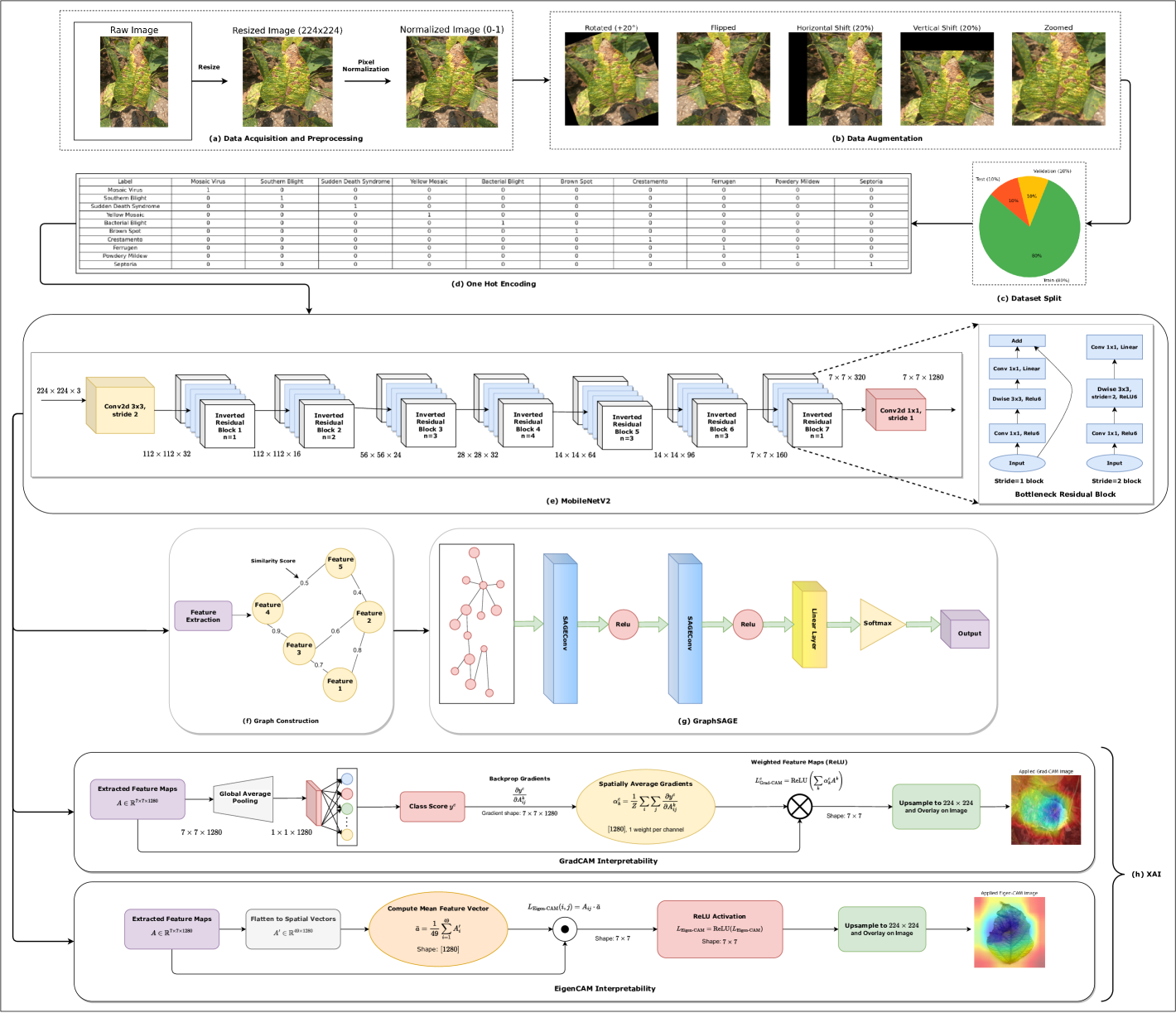
Figure 1: Proposed Sequential MobileNetV2-GraphSAGE framework: (a) Images are resized to $224\times 224$ pixels and normalized. (b) Data augmentation includes rotation, flipping, shifting, and zooming. (c) Dataset is split (80%-10%-10%) for training, validation, and testing. (d) Disease labels are one-hot encoded. (e) MobileNetV2 extracts local features. (f) Graph construction captures relationships. (g) GraphSAGE aggregates neighborhood information. (h) Cross-modal interpretation uses Grad-CAM and Eigen-CAM.

III Methodology

This section outlines the methodology used in this work for classifying soybean leaf diseases using a Sequential CNN-GNN model. The overall pipeline consisting of data preprocessing, augmentation, and model development used in this study is illustrated in Figure 1. The pipeline consists of several key steps, including image acquisition, resizing, pixel normalization, augmentation, dataset splitting, and one-hot encoding, ensuring a standardized dataset for training and evaluation. During model development, images are first passed through a MobileNetV2 architecture to extract local features. These features are then structured into a graph, with edges representing the relationships between image features. GraphSAGE is used to aggregate neighborhood information and capture global dependencies within the data. Finally, the aggregated features are fed into a classifier to predict soybean leaf diseases. This integrated approach ensures local feature extraction and global dependency modeling, leveraging the strengths of both CNN and GNN architectures for improved disease classification.

III-A Model Framework and Architecture

The proposed Sequential CNN-GNN model combines a CNN for extracting local features from images and a GNN for capturing the relationships between these features. The model is designed in a sequential manner: the CNN first extracts detailed local features, and then the GNN processes these features to understand global dependencies, enhancing classification accuracy.

The model begins by taking an input image $I\in\mathbb{R}^{H\times W\times C}$, where $H$, $W$, and $C$ represent the height, width, and the number of channels (3 for RGB). The input image is first passed through the MobileNetV2 CNN, which is known for its efficiency and low computational cost. MobileNetV2 uses depthwise separable convolutions, reducing the number of parameters and operations compared to traditional convolutions. This makes it ideal for extracting local features efficiently.

The output from the MobileNetV2 CNN is a set of feature maps $F_{\text{cnn}}\in\mathbb{R}^{H^{\prime}\times W^{\prime}\times C^{\prime}}$, where $H^{\prime}$, $W^{\prime}$, and $C^{\prime}$ represent the spatial dimensions and depth of the extracted feature maps. These feature maps are then normalized to a range between 0 and 1 by dividing by 255, ensuring consistent scaling across the dataset:

$$F_{\text{cnn}}=\frac{F_{\text{cnn}}}{255}$$ (1)

These normalized feature maps serve as input for the GNN branch, where each feature map is treated as a node in a graph. To construct the graph, we calculate the cosine similarity between feature vectors from different image patches to measure their relationships. The similarity between two feature vectors $F_{i}$ and $F_{j}$ is computed as:

$$S_{ij}=\frac{F_{i}\cdot F_{j}}{\|F_{i}\|\|F_{j}\|}$$ (2)

where $\|F_{i}\|$ and $\|F_{j}\|$ are the L2 norms of $F_{i}$ and $F_{j}$, respectively. An adjacency matrix $A$ is constructed based on these similarities. If the similarity between two nodes exceeds a threshold $\theta$, we set $A_{ij}=1$; otherwise, $A_{ij}=0$. This adjacency matrix defines how the nodes (image patches) are connected in the graph.

GraphSAGE is then used to aggregate information from the neighbors of each node. Unlike traditional GNNs, which aggregate information from all neighboring nodes, GraphSAGE performs neighborhood sampling to handle large graphs efficiently. The feature update rule for a node $H^{(k+1)}$ at the $(k+1)$-th layer is as follows:

$$H^{(k+1)}=\sigma\left(\hat{A}H^{(k)}W^{(k)}\right)$$ (3)

where $H^{(k)}\in\mathbb{R}^{N\times F_{k}}$ is the feature matrix at the $k$-th layer, with $N$ nodes and $F_{k}$ features per node. $\hat{A}$ is the normalized adjacency matrix (with self-loops added), and $W^{(k)}\in\mathbb{R}^{F_{k}\times F_{k+1}}$ is the learnable weight matrix at layer $k$. $\sigma$ is the non-linear activation function (typically ReLU).

GraphSAGE aggregates the features of neighboring nodes using a sampling-based approach and iteratively updates the node features to capture both local and global information. After several layers of graph convolutions, the final node features $H^{(K)}$ are passed through a softmax layer to compute the class probabilities:

$$\hat{y}=\text{softmax}(H^{(K)})$$ (4)

These probabilities represent the likelihood of each class for the image.

III-A1 Sequential Architecture

The architecture of the Sequential CNN-GNN model combines the strengths of both CNNs and GNNs. The CNN branch captures local image patterns, while the GraphSAGE-based GNN branch aggregates information from neighboring patches to understand global relationships. This sequential structure allows the model to leverage local and global feature representations, making it particularly effective for complex image classification tasks, such as soybean leaf disease identification.

1. Input: The model accepts an image $I\in\mathbb{R}^{H\times W\times C}$.

2. CNN Branch: MobileNetV2 extracts local features, resulting in feature maps $F_{\text{cnn}}\in\mathbb{R}^{H^{\prime}\times W^{\prime}\times C^{\prime}}$.

3. GNN Branch: The feature maps are treated as nodes in a graph. The adjacency matrix $A$ is constructed using cosine similarity, and the GraphSAGE algorithm updates the node features through graph convolutions.

4. Output: The final node features are passed through a softmax layer to output class probabilities.

III-B Feature Extraction Techniques

The feature extraction step leverages MobileNetV2, a lightweight convolutional neural network architecture specifically designed for efficient image classification tasks, particularly in resource-constrained environments. MobileNetV2 utilizes depthwise separable convolutions, significantly reducing computational complexity and the number of parameters while maintaining high performance. This makes MobileNetV2 especially effective for extracting meaningful local features from images without incurring high computational costs, which is crucial for large-scale agricultural datasets.

For the soybean leaf disease classification task, MobileNetV2 effectively captures local image features, which are essential for distinguishing between different leaf disease types. Mathematically, the feature extraction process can be represented as:

$$F_{\text{cnn}}=\text{MobileNetV2}(I)$$ (5)

where $F_{\text{cnn}}\in\mathbb{R}^{H^{\prime}\times W^{\prime}\times C^{\prime}}$ represents the feature map extracted from the input image $I$, with $H^{\prime}$, $W^{\prime}$, and $C^{\prime}$ denoting the spatial dimensions and depth of the extracted features.

After the extraction, the feature maps undergo normalization to ensure the pixel values fall within the range [0, 1]. This normalization step standardizes the subsequent GNN input, ensuring consistent scaling across the dataset. This consistency is crucial for improving model convergence during training and helping the model learn more effectively.

III-C Graph Construction and Representation

After feature extraction, each feature map $F_{\text{cnn}}$ is treated as a node in the graph. The relationship between these nodes is modeled by computing the cosine similarity between the feature vectors extracted from different image patches. This similarity helps to capture the structural and semantic relationships between the image regions, which is critical for understanding global dependencies.

The adjacency matrix $A$ is then constructed based on these cosine similarities. Each element $A_{ij}$ in the matrix represents the relationship between nodes $i$ and $j$, with higher values indicating a stronger relationship. To simplify the graph structure, we threshold the cosine similarity to form a binary adjacency matrix:

$$A_{ij}=\begin{cases}1&\text{if }S_{ij}>\theta\\ 0&\text{otherwise}\end{cases}$$ (6)

where $S_{ij}$ denotes the cosine similarity between nodes $i$ and $j$, and $\theta$ is the similarity threshold. The threshold $\theta$ controls how strongly nodes must be related to be connected in the graph. This binary representation helps reduce complexity while preserving the most meaningful relationships. This graph structure enables the GNN to model and learn the interdependencies between image patches, capturing local and global patterns for enhanced classification performance.

III-D Optimization Methods and Loss Function

The model is trained using categorical cross-entropy as the loss function, which is suitable for multi-class classification. The loss function is defined as:

$$L=-\sum_{i}y_{i}\log(\hat{y_{i}})$$ (7)

where $y_{i}$ is the true class label for the $i$-th image, and $\hat{y_{i}}$ is the predicted probability for class $i$.

We use the Adam optimizer with a learning rate of 0.001 for model optimization, as it is efficient and adapts the learning rate during training. Dropout is applied to fully connected layers to prevent overfitting, with a dropout rate of 0.5.

III-E Model Training and Evaluation

The model was trained using an 80%-20% data split, with 80% of the dataset allocated for training and 20% for testing. A batch size 32 was used, and training was conducted for 20 epochs to ensure sufficient learning. The model’s performance was evaluated using standard classification metrics, including accuracy, precision, recall, and F1 score. Accuracy represents the percentage of correctly classified samples, while precision measures the proportion of correctly predicted positive instances out of all predicted positives. Recall quantifies the model’s ability to identify all actual positive cases, and the F1 score provides a balanced measure by computing the harmonic mean of precision and recall.

III-F Mathematical Formulations

GraphSAGE updates node features through a neighborhood sampling and aggregation process designed to efficiently handle large-scale graphs. Instead of directly using the entire adjacency matrix, GraphSAGE samples a fixed-size set of neighboring nodes for each target node at every layer. For a given node $v$ at layer $k$, its feature representation is updated by aggregating the feature vectors of its sampled neighbors. This aggregation can be performed using different strategies such as mean aggregation, pooling, or an LSTM-based aggregator. The aggregated neighbor features are then concatenated with the current node’s own features, and the concatenated vector is passed through a learnable linear transformation followed by a non-linear activation function (typically ReLU). Mathematically, the feature update at layer $k$ can be expressed as:

$$h_{v}^{(k+1)}=\sigma\left(W^{(k)}\cdot\text{AGGREGATE}\left(\{h_{u}^{(k)}:u\in\mathcal{N}(v)\}\right)\,\|\,h_{v}^{(k)}\right)$$ (8)

where $h_{v}^{(k)}$ denotes the feature vector of node $v$ at layer $k$, $\mathcal{N}(v)$ denotes the sampled neighborhood of node $v$, $W^{(k)}$ is a trainable weight matrix, $\sigma$ is a non-linear activation function, and $\|$ denotes the concatenation operation. This sampling and aggregation process allows GraphSAGE to efficiently scale to large graphs while maintaining flexibility in how neighbor information is combined. After $K$ layers of neighborhood aggregation, the final node embeddings $h_{v}^{(K)}$ can be directly used for downstream tasks such as node classification, where they are passed through a softmax layer to compute class probabilities:

$$\hat{y}_{v}=\text{softmax}(h_{v}^{(K)})$$ (9)

This formulation allows GraphSAGE to learn expressive node representations while being computationally efficient, as it avoids the need to process all neighbors at every step, unlike traditional GCNs.

III-G Innovative Techniques

The proposed model leverages a hybrid architecture that combines MobileNetV2 with GraphSAGE, capitalizing on the complementary strengths of CNNs and GNNs. MobileNetV2 is a lightweight feature extractor, efficiently capturing fine-grained local patterns from the input image through depthwise separable convolutions. These extracted features are then transformed into graph-structured data, where GraphSAGE aggregates information from neighboring nodes, enabling the model to learn spatial and semantic relationships between localized regions. This explicit modeling of local texture details and global relational dependencies enhances the model’s ability to distinguish subtle variations between disease patterns, particularly in cases where visual symptoms exhibit spatial spread or irregular clustering. Compared to traditional CNN pipelines, this hybrid design reduces reliance on large convolutional stacks, improving computational efficiency while enhancing spatial reasoning — a limitation in purely convolutional architectures. Moreover, unlike GCN and GAT, which assume fixed graph structures or require dense attention computations, GraphSAGE’s sampling-based neighborhood aggregation balances performance and scalability, making it well-suited for irregular and incomplete spatial patterns common in leaf disease imaging. This combination of efficient feature extraction, flexible graph modeling, and reduced computational overhead positions the proposed approach as a robust alternative to standalone CNN, standalone GNN, parallel CNN-GNN connection, and other hybrid CNN-GNN variants.

IV Experiments

IV-A Datasets and Preprocessing

The dataset utilized in this study comprises high-quality images of soybean leaves affected by ten different diseases, including Mosaic Virus, Southern Blight, Sudden Death Syndrome, Yellow Mosaic, Bacterial Blight, Brown Spot, Crestamento, Ferrugen, Powdery Mildew, and Septoria. The dataset is well-labeled and encompasses a diverse range of real-world conditions, making it highly suitable for plant disease classification tasks. To ensure consistency in the input size, all images were resized to $224\times 224$ pixels. Pixel values were normalized by scaling them between 0 and 1, achieved by dividing by 255. Data augmentation techniques, such as random rotation up to $20^{\circ}$, horizontal flipping, width and height shifts of 20%, and zooming, were applied to enhance model robustness. The dataset was partitioned into 80% training and 20% testing, with 10% of the total dataset reserved for validation during training, while the remaining 10% was utilized for final testing. Furthermore, the categorical disease labels were one-hot encoded to facilitate multi-class classification. These preprocessing steps ensured the model was trained on standardized and augmented data, improving its ability to generalize effectively to unseen samples.

IV-B Experimental Configuration

The experiments were conducted using a GPU $T4\times 2$ setup to enable efficient and accelerated training. The deep learning framework utilized for model development was TensorFlow 2.x with Keras, along with essential libraries such as NumPy, Matplotlib, and Scikit-learn. The implementation was done in Python 3.8. The training process employed the Adam optimizer with a learning rate of 0.001, a batch size of 32, and 20 epochs. To mitigate overfitting, a dropout rate of 0.5 was applied to the fully connected layers. The model’s performance was evaluated using accuracy, precision, recall, and F1 score. To assess the effectiveness of the Sequential CNN-GNN model, we conducted comparisons against baseline models and performed ablation tests.

IV-C Evaluation Strategy

To demonstrate the benefits of integrating local feature extraction from CNNs with global relational reasoning from GNNs, we compare the proposed model against a diverse set of baselines, including traditional machine learning models (Support Vector Classifier, Random Forest, Logistic Regression, K-Nearest Neighbors), standalone CNNs (MobileNetV2, EfficientNetB0, ResNet50, VGG16, VGG19, Xception, DenseNet family, InceptionV3, NASNetLarge, and ResNet variants), and hybrid combinations of CNNs and GNNs (GCN, GAT, and GraphSAGE). This comprehensive evaluation highlights the strengths and limitations of each architecture, particularly the ability of the MobileNetV2-GraphSAGE combination to balance lightweight feature extraction with neighborhood-aware reasoning. To ensure fairness and reproducibility, all models were trained and evaluated under the same conditions, using identical batch size, learning rate, optimizer, number of epochs, data augmentation pipeline, and training-validation-test splits. This consistent experimental setup ensures that performance differences reflect genuine architectural advantages rather than variations in training protocols.

V Results and Discussion

V-A Performance Comparison

The benchmarking results, as shown in Table I, provide critical insights into the performance of various CNN-GNN hybrid models for soybean leaf disease classification. Among the tested models, MobileNetV2 + GraphSAGE and InceptionV3 + GraphSAGE achieved the highest accuracy of 97.16%, with MobileNetV2 + GraphSAGE showing a slight edge in precision (97.51%) and InceptionV3 + GraphSAGE excelling in F1-score (97.06%). These results indicate that integrating GraphSAGE with lightweight CNN architectures can significantly enhance classification performance. On the other hand, traditional machine learning models like SVC, Random Forest, Logistic Regression, and KNN showed significantly lower performance, with accuracies ranging from 66.39% to 77.05%. These results highlight the superiority of deep learning models, particularly the Sequential CNN-GNN, over traditional machine learning models for this image classification task.

GraphSAGE consistently outperformed GCN and GAT across all CNN backbones, highlighting its superior capability in extracting meaningful graph-based features. While deeper CNN architectures like DenseNet201 and DenseNet169 also demonstrated strong results, achieving accuracy above 96%, their performance was slightly below the best-performing models. EfficientNetB0 exhibited extremely poor results ($\approx$15.6% accuracy) across all GNN variants, indicating its inefficacy in this classification task.

Furthermore, ResNet101 and ResNet152 performed poorly with GCN but improved significantly with GraphSAGE and GAT, emphasizing the importance of selecting the right GNN variant for a given CNN backbone. Overall, the results confirm that combining lightweight CNNs with GraphSAGE offers the most effective approach for soybean leaf disease classification. Among the models, MobileNetV2 + GraphSAGE stands out as the proposed model due to its superior balance between accuracy, computational efficiency, and ease of deployment. While InceptionV3 + GraphSAGE achieved similar accuracy, MobileNetV2’s lightweight architecture makes it more suitable for real-world applications, particularly in resource-constrained environments where efficiency and scalability are critical.

According to Table III, traditional CNNs like ResNet, VGG, Inception, and NASNet have larger parameter counts, with NASNetLarge at 84.9M. These models are more complex and resource-intensive. MobileNetV2 and EfficientNetB0 are lightweight models with 2-4M parameters, which are ideal for mobile or edge devices. DenseNet models (7M to 18M parameters) feature dense connectivity for better information flow with moderate size. GCN, GAT, and GraphSAGE, with 10K to 67K parameters, are specialized for graph tasks and have much fewer parameters than CNNs. Larger models like InceptionV3 and ResNet152 offer high performance but require more resources, while smaller models like MobileNetV2 balance performance and efficiency.

TABLE I: Benchmarking Results on Soybean Leaf Disease Dataset. Bold indicates the best performance and Underline indicates the second best performance.

Model	Accuracy ($\uparrow$)	Precision ($\uparrow$)	Recall ($\uparrow$)	F1 Score ($\uparrow$)
SVC	77.05%	76.00%	77.05%	73.65%
RandomForest	77.05%	74.86%	77.05%	73.65%
Logistic Regression	77.05%	73.39%	77.05%	74.42%
KNN	66.39%	70.00%	66.39%	61.21%
MobileNetV2	93.62%	93.75%	93.62%	92.77%
MobileNetV2 + GCN	95.74%	95.60%	95.74%	95.46%
MobileNetV2 + GAT	96.45%	96.89%	96.45%	96.11%
MobileNetV2 + GraphSAGE	97.16%	97.51%	97.16%	96.79%
EfficientNetB0	19.86%	3.94%	19.86%	6.58%
EfficientNetB0 + GCN	15.60%	2.43%	15.60%	4.21%
EfficientNetB0 + GAT	15.60%	2.43%	15.60%	4.21%
EfficientNetB0 + GraphSAGE	15.60%	2.43%	15.60%	4.21%
ResNet50	47.52%	35.18%	47.52%	36.20%
ResNet50 + GCN	50.35%	45.06%	50.35%	43.79%
ResNet50 + GAT	62.41%	61.20%	62.41%	57.48%
ResNet50 + GraphSAGE	63.12%	63.81%	63.12%	58.90%
VGG16	82.98%	80.23%	82.98%	79.29%
VGG16 + GCN	94.33%	91.88%	94.33%	93.03%
VGG16 + GAT	94.33%	92.62%	94.33%	93.36%
VGG16 + GraphSAGE	93.62%	91.44%	93.62%	92.38%
VGG19	80.14%	78.19%	80.14%	76.14%
VGG19 + GCN	95.04%	91.97%	95.04%	93.40%
VGG19 + GAT	92.20%	90.03%	92.20%	90.78%
VGG19 + GraphSAGE	95.04%	91.97%	95.04%	93.40%
Xception	92.20%	92.78%	92.20%	91.20%
Xception + GCN	94.33%	94.81%	94.33%	94.34%
Xception + GAT	95.04%	95.26%	95.04%	94.96%
Xception + GraphSAGE	95.04%	95.13%	95.04%	94.95%
DenseNet121	92.91%	92.76%	92.91%	92.37%
DenseNet121 + GCN	93.62%	91.69%	93.62%	92.45%
DenseNet121 + GAT	95.04%	95.65%	95.04%	94.70%
DenseNet121 + GraphSAGE	95.74%	95.45%	95.74%	95.45%
DenseNet169	92.91%	90.43%	92.91%	91.15%
DenseNet169 + GCN	96.45%	96.11%	96.45%	96.14%
DenseNet169 + GAT	95.74%	94.96%	95.74%	95.27%
DenseNet169 + GraphSAGE	96.45%	96.73%	96.45%	95.59%
DenseNet201	95.04%	93.03%	95.04%	93.75%
DenseNet201 + GCN	94.33%	94.17%	94.33%	93.82%
DenseNet201 + GAT	97.16%	96.87%	97.16%	96.87%
DenseNet201 + GraphSAGE	96.45%	96.32%	96.45%	96.20%
InceptionV3	92.20%	92.10%	92.20%	91.73%
InceptionV3 + GCN	96.45%	96.70%	96.45%	96.05%
InceptionV3 + GAT	95.04%	95.55%	95.04%	94.21%
InceptionV3 + GraphSAGE	97.16%	97.46%	97.16%	97.06%
InceptionResNetV2	90.07%	87.73%	90.07%	87.92%
NASNetLarge	89.36%	90.10%	89.36%	87.96%
NASNetLarge + GCN	92.91%	93.59%	92.91%	92.95%
NASNetLarge + GAT	91.49%	91.41%	91.49%	91.33%
NASNetLarge + GraphSAGE	91.49%	91.57%	91.49%	91.27%
NASNetMobile	91.49%	91.40%	91.49%	91.08%
ResNet101	46.10%	45.24%	46.10%	36.43%
ResNet101 + GCN	62.41%	66.52%	62.41%	56.18%
ResNet101 + GAT	77.30%	74.59%	77.30%	72.90%
ResNet101 + GraphSAGE	80.85%	79.69%	80.85%	78.11%
ResNet152	57.45%	43.31%	57.45%	48.26%
ResNet152 + GCN	65.25%	57.83%	65.25%	58.55%
ResNet152 + GAT	68.79%	62.10%	68.79%	62.66%
ResNet152 + GraphSAGE	55.32%	67.60%	55.32%	51.35%
ResNet50V2	95.04%	94.78%	95.04%	94.30%
ResNet50V2 + GCN	94.33%	95.13%	94.33%	93.55%
ResNet50V2 + GAT	95.74%	95.96%	95.74%	95.69%
ResNet50V2 + GraphSAGE	94.33%	94.49%	94.33%	94.12%

TABLE II: Ablation Study of Sequential CNN-GNN Model

Model Variant	Accuracy ($\uparrow$)	Precision ($\uparrow$)	Recall ($\uparrow$)	F1 Score ($\uparrow$)
MobileNetV2 w/o GraphSAGE	93.62%	93.75%	93.62%	92.77%
GraphSAGE w/o MobileNetV2	91.30%	90.76%	91.30%	90.22%
MobileNetV2 + GraphSAGE (Parallel)	95.74%	96.36%	95.74%	94.96%
GNN + MobileNetV2 (Sequential)	96.45%	97.07%	96.45%	95.67%
Sequential MobileNetV2 + GraphSAGE (Proposed)	97.16%	97.51%	97.16%	96.79%

TABLE III: CNN and GNN Models and their Parameter Counts

Model	Parameter Count ($\downarrow$)
MobileNetV2	2,257,984
EfficientNetB0	4,049,571
ResNet50	23,587,712
VGG16	14,714,688
VGG19	20,024,384
Xception	20,861,480
DenseNet121	7,037,504
DenseNet169	12,642,880
DenseNet201	18,321,984
InceptionV3	21,802,784
NASNetLarge	84,916,818
ResNet101	42,658,176
ResNet152	58,370,944
ResNet50V2	23,564,800
GCN	10,666
GAT	25,418
GraphSAGE	67,210
MobileNetV2+GraphSAGE	2,325,194

V-B Ablation Studies

To better understand the contribution of each component of the proposed model, we conducted an ablation study, the results of which are summarized in Table II. The study evaluates the performance of different model variants, including MobileNetV2 w/o GraphSAGE, GraphSAGE w/o MobileNetV2, and other combinations.

1. The MobileNetV2 w/o GraphSAGE variant, which only uses MobileNetV2 for feature extraction, achieved an accuracy of 93.62%.

2. The GraphSAGE w/o MobileNetV2 variant, which uses only GraphSAGE for feature aggregation, achieved an accuracy of 91.30%.

3. The MobileNetV2 + GraphSAGE (Parallel) model, where MobileNetV2 and GraphSAGE are applied in parallel, resulted in an accuracy of 95.74%.

4. The GraphSAGE + MobileNetV2 (Sequential) model, where GraphSAGE is applied after MobileNetV2, achieved an accuracy of 97.16%.

The proposed Sequential MobileNetV2+GraphSAGE model outperformed all other variants, with an accuracy of 97.16%, demonstrating that the sequential combination of MobileNetV2 and GraphSAGE is the most effective approach for this task. This ablation study highlights the importance of both components working together in a sequential manner rather than independently or in parallel.

V-C Interpretability

The interpretability of the model was evaluated using Grad-CAM and Eigen-CAM to visualize the regions of the images that contribute most to the model’s decisions. These techniques allow us to understand which parts of the soybean leaves the model focuses on when classifying diseases.

The Grad-CAM visualizations, shown in Figure 2, indicate that the model primarily focuses on the areas of the leaves that show clear signs of disease, such as lesions, spots, and discoloration. The figure shows the original images (top row) alongside the corresponding Grad-CAM heatmaps (bottom row), highlighting the areas of interest that influence the model’s classification decision. The Eigen-CAM visualizations, shown in Figure 3, further help identify the key features associated with each disease type, confirming that the model learns discriminative features essential for accurate classification. The Eigen-CAM heatmaps provide a detailed view of how the model interprets different features within the leaf images. These visualizations provide confidence in the model’s decision-making process and demonstrate its ability to focus on relevant image patterns, making it more interpretable and trustworthy.

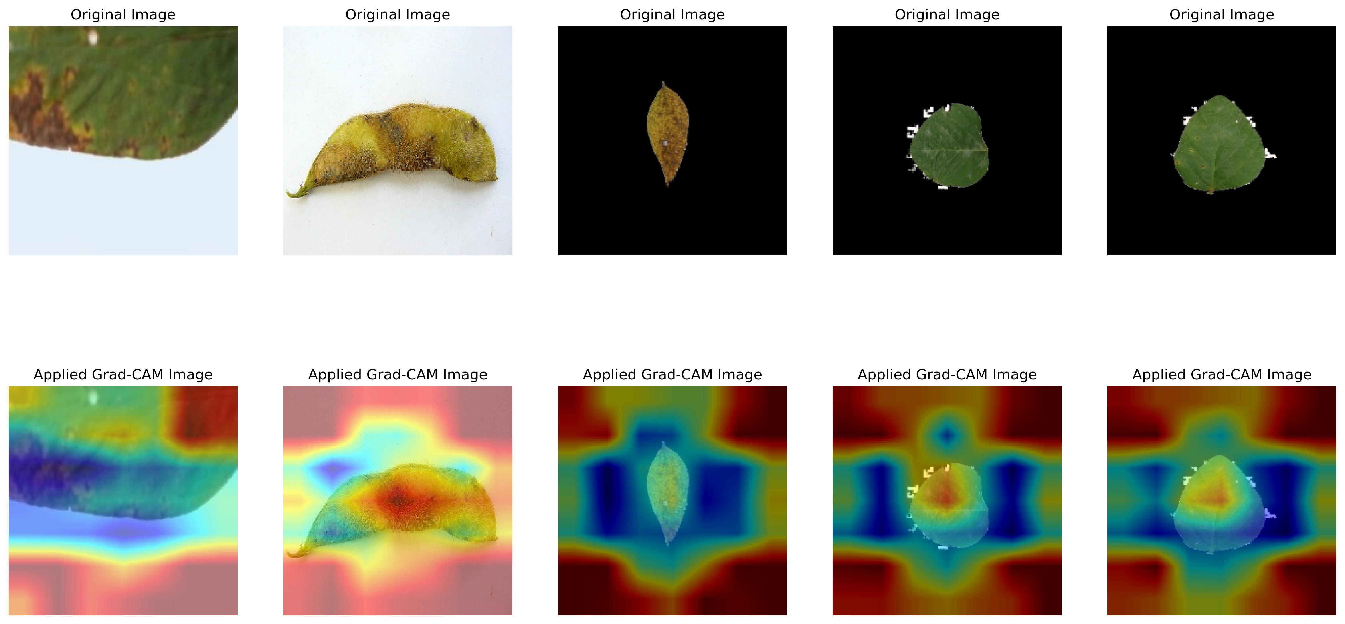
Figure 2: Grad-CAM Visualizations. The figure shows the original images (top row) alongside the corresponding Grad-CAM heatmaps (bottom row), highlighting the areas of interest that influence the model’s classification decision.

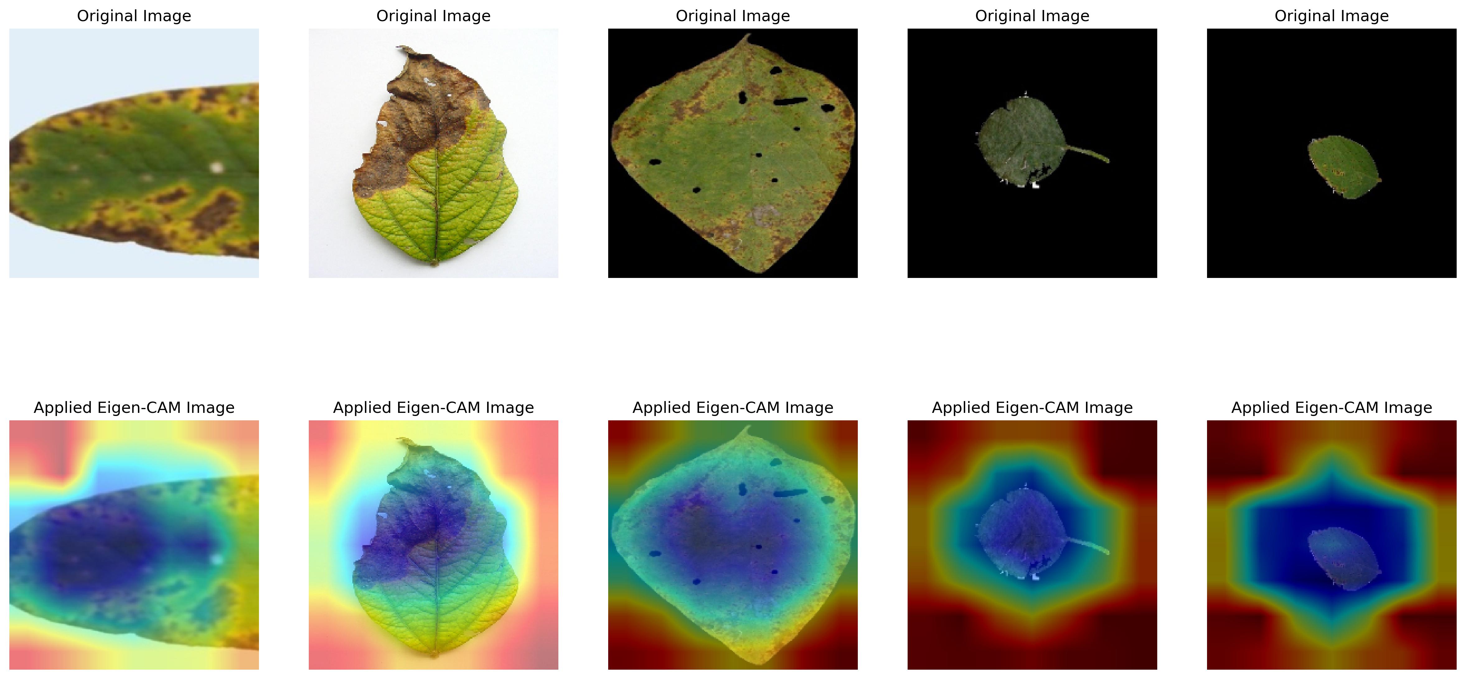
Figure 3: Eigen-CAM Visualizations. The figure shows the original images (top row) and the applied Eigen-CAM heatmaps (bottom row), providing a detailed view of how the model interprets different features within the leaf images.

VI Conclusion and Future Work

This work presented a hybrid soybean leaf disease detection framework, combining MobileNetV2 for efficient feature extraction and GraphSAGE for capturing symptom relationships. The resulting MobileNetV2 + GraphSAGE model achieved 97.16% accuracy, 97.51% precision, and 96.79% F1 score, outperforming alternative architectures while maintaining low computational cost and fast inference, which are the key factors for deployment in mobile and edge environments. Grad-CAM and Eigen-CAM provided further insights into visual and relational features driving predictions, enhancing the model’s interpretability and trustworthiness for real-world use. This approach underscores the potential of integrating GNNs with lightweight CNNs for efficient, scalable plant disease detection.

Future work will focus on improving generalization through expanded datasets incorporating environmental variables (e.g., soil, climate), optimizing the model via pruning and quantization, and investigating advanced architectures like attention-based and multi-modal models. Using TensorFlow Lite and ONNX deployment strategies will ensure real-time performance on resource-constrained devices, enabling practical smart farming solutions.

References

- [1] J. Chen, J. Chen, D. Zhang, Y. Sun, and Y. A. Nanehkaran, “Using deep transfer learning for image-based plant disease identification,” Computers and electronics in agriculture, vol. 173, p. 105393, 2020, publisher: Elsevier.
- [2] P. K. Sethy, N. K. Barpanda, A. K. Rath, and S. K. Behera, “Deep feature based rice leaf disease identification using support vector machine,” Computers and Electronics in Agriculture, vol. 175, p. 105527, 2020, publisher: Elsevier.
- [3] S. Dou, L. Wang, D. Fan, L. Miao, J. Yan, and H. He, “Classification of Citrus Huanglongbing Degree based on CBAM-MobileNetV2 and transfer learning,” Sensors, vol. 23, no. 12, p. 5587, 2023, publisher: MDPI.
- [4] G. Sheng, W. Min, T. Yao, J. Song, Y. Yang, L. Wang, and S. Jiang, “Lightweight food image recognition with global shuffle convolution,” IEEE Transactions on AgriFood Electronics, vol. 2, no. 2, pp. 392–402, 2024.
- [5] A. Bera, O. Krejcar, and D. Bhattacharjee, “Rafa-net: Region attention network for food items and agricultural stress recognition,” IEEE Transactions on AgriFood Electronics, pp. 1–13, 2024.
- [6] M. A. Rahman, A. A. Khan, M. M. Hasan, M. S. Rahman, and M. T. Habib, “Deep learning modeling for potato breed recognition,” IEEE Transactions on AgriFood Electronics, vol. 2, no. 2, pp. 419–427, 2024.
- [7] S. Janarthan, S. Thuseethan, S. Rajasegarar, Q. Lyu, Y. Zheng, and J. Yearwood, “Liran: A lightweight residual attention network for in-field plant pest recognition,” IEEE Transactions on AgriFood Electronics, pp. 1–12, 2024.
- [8] X. Wang, D. Wang, Z. He, Z. Lin, and S. Xie, “Ama-net: Adaptive masking attention network for agricultural crop classification from uav images,” IEEE Transactions on AgriFood Electronics, pp. 1–8, 2025.
- [9] J. Wu, V. Abolghasemi, M. H. Anisi, U. Dar, A. Ivanov, and C. Newenham, “Strawberry disease detection through an advanced squeeze-and-excitation deep learning model,” IEEE Transactions on AgriFood Electronics, vol. 2, no. 2, pp. 259–267, 2024.
- [10] A. Karlekar and A. Seal, “Soynet: Soybean leaf diseases classification,” Computers and Electronics in Agriculture, vol. 172, p. 105342, 2020.
- [11] Q. Wu, X. Ma, H. Liu, C. Bi, H. Yu, M. Liang, J. Zhang, Q. Li, Y. Tang, and G. Ye, “A classification method for soybean leaf diseases based on an improved convnext model,” Scientific Reports, vol. 13, no. 1, p. 19141, 2023.
- [12] R. B. D. T. Senthil Prakash, Vandana C. P. and A. Kiran, “Auto-metric graph neural network for paddy leaf disease classification,” Archives of Phytopathology and Plant Protection, vol. 56, no. 19, pp. 1487–1508, 2023.
- [13] D. Li, “Application of Deep Reinforcement Learning Based Graph Convolutional Neural Network for Sugarcane Leaf Disease Identification,” in Proceedings of the 2023 5th International Conference on Internet of Things, Automation and Artificial Intelligence, ser. IoTAAI ’23. New York, NY, USA: Association for Computing Machinery, 2024, p. 13–17.
- [14] W. Hamilton, Z. Ying, and J. Leskovec, “Inductive Representation Learning on Large Graphs,” in Advances in Neural Information Processing Systems, vol. 30. Curran Associates, Inc., 2017.
- [15] P. B. Padol and A. A. Yadav, “SVM classifier based grape leaf disease detection,” in 2016 Conference on advances in signal processing (CASP). IEEE, 2016, pp. 175–179.
- [16] A. H. Kulkarni and A. Patil, “Applying image processing technique to detect plant diseases,” International Journal of Modern Engineering Research, vol. 2, no. 5, pp. 3661–3664, 2012, publisher: Citeseer.
- [17] R. Rayhana, Z. Ma, Z. Liu, G. Xiao, Y. Ruan, and J. S. Sangha, “A review on plant disease detection using hyperspectral imaging,” IEEE Transactions on AgriFood Electronics, vol. 1, no. 2, pp. 108–134, 2023.
- [18] T. N. Kipf and M. Welling, “Semi-Supervised Classification with Graph Convolutional Networks,” in Proceedings of the 5th International Conference on Learning Representations, ser. ICLR’17, 2017.
- [19] W. L. Hamilton, R. Ying, and J. Leskovec, “Inductive representation learning on large graphs,” in Proceedings of the 31st International Conference on Neural Information Processing Systems, ser. NIPS’17. Red Hook, NY, USA: Curran Associates Inc., 2017, p. 1025–1035.
- [20] D. Ahmedt-Aristizabal, M. A. Armin, S. Denman, C. Fookes, and L. Petersson, “Graph-Based Deep Learning for Medical Diagnosis and Analysis: Past, Present and Future,” Sensors (Basel, Switzerland), vol. 21, no. 14, p. 4758, July 2021.
- [21] D. Kavran, D. Mongus, B. Žalik, and N. Lukač, “Graph neural network-based method of spatiotemporal land cover mapping using satellite imagery,” Sensors, vol. 23, no. 14, 2023.
- [22] P. Thangamariappan, M. Singh, M. Arthi, T. Kannan, and S. Saraswathy, “Enhanced structural image classification using hybrid cnn-gnn model,” in 2024 International Conference on Knowledge Engineering and Communication Systems (ICKECS), vol. 1, 2024, pp. 1–6.
- [23] G. Nikolentzos, M. Thomas, A. R. Rivera, and M. Vazirgiannis, “Image classification using graph-based representations and graph neural networks,” in Complex Networks & Their Applications IX, R. M. Benito, C. Cherifi, H. Cherifi, E. Moro, L. M. Rocha, and M. Sales-Pardo, Eds. Cham: Springer International Publishing, 2021, pp. 142–153.
- [24] Y. Zhang, X. Song, Z. Hua, and J. Li, “Cgmma: Cnn-gnn multiscale mixed attention network for remote sensing image change detection,” IEEE Journal of Selected Topics in Applied Earth Observations and Remote Sensing, vol. 17, pp. 7089–7103, 2024.
- [25] T. Tang, X. Chen, Y. Wu, S. Sun, and M. Yu, “Image classification based on deep graph convolutional networks,” in 2022 IEEE 9th International Conference on Data Science and Advanced Analytics (DSAA), 2022, pp. 1–6.