Online Learning of Nonlinear Parametric Models under Non-smooth Regularization using EKF and ADMM

Abstract

This paper proposes a novel combination of extended Kalman filtering (EKF) with the alternating direction method of multipliers (ADMM) for learning parametric nonlinear models online under non-smooth regularization terms, including $\ell_{1}$ and $\ell_{0}$ penalties and bound constraints on model parameters. For the case of linear time-varying models and non-smooth convex regularization terms, we provide a sublinear regret bound that ensures the proper behavior of the online learning strategy. The approach is computationally efficient for a wide range of regularization terms, which makes it appealing for its use in embedded control applications for online model adaptation. We show the performance of the proposed method in three simulation examples, highlighting its effectiveness compared to other batch and online algorithms.

Keywords Kalman filtering  $\cdot$ non-smooth regularization  $\cdot$ online learning  $\cdot$ parameter estimation  $\cdot$ adaptive control  $\cdot$ neural networks.

1 Introduction

Online learning of nonlinear parametric models is of paramount importance in several domains, including model-based adaptive control and real-time estimation of unmeasured variables. Typically, parametric models derived from physics [1] or black-box [2] structures are identified offline on training data, then directly deployed and used without any further updates. On the other hand, further adapting the model online can significantly improve its predictive capabilities [3], especially when the phenomenon we are modeling changes over time. Moreover, online model learning allows for smaller model structures that adapt to varying operating conditions, unlike single, overall models trained offline to cover all conditions.

A vast literature currently exists for online learning [4] and several approaches have been investigated, such as stochastic gradient descent (SGD) [5], follow-the-regularized-leader (FTRL) [6], and online ADMM (alternating direction method of multipliers) [7]. While such approaches provide reasonable learning performance with limited computational effort and can deal with quite general loss functions and regularization terms, they usually learn very slowly, which might be a critical issue, for example, in adaptive control applications.

By treating parameters as constant states, extended Kalman filtering (EKF) has also been proven to be an effective strategy for recursively adapting models from measurements [8, 9, 10, 11, 12, 13] with a faster convergence rate [14]. In particular, [12] proposed a modification of the classical EKF to deal with forgetting factors and an exponential moving-average regularization, improving the performance and flexibility of the online parameter estimation setting, while [11] investigated the use of EKF for the online training of neural network models under general smooth convex losses and smooth regularization functions, with $\ell_{1}$-regularization treated as a special limit case of a smooth regularization. In fact, the main limitation of EKF is that it requires quadratic approximations of nonlinear penalty functions to be able to rephrase the penalty as a squared Euclidean norm of a properly-defined measurement error. This limitation makes EKF not directly suitable for dealing with general non-smooth regularization terms, such as $\ell_{0}$ regularization, group-Lasso penalties, and bound constraints on model parameters, which could instead be beneficial to reduce the complexity of the learned model.

In this paper, we propose a simple and computationally efficient modification of the EKF algorithm by intertwining updates based on online measurements and output prediction errors with updates related to ADMM iterations. This modification allows EKF to deal with a broad class of non-smooth regularization terms for which ADMM is applicable, including $\ell_{0}$/$\ell_{1}$ penalties and bound constraints on model parameters. For linear time-varying models and convex regularization terms, we provide a sublinear regret bound that proves the proper behavior of the resulting online learning strategy. The proposed method is computationally efficient and numerically robust, making it especially appealing for embedded adaptive control applications.

The rest of the paper is organized as follows. Section 2 gives a quick introduction to the use of EKF for online model learning, setting the background for the proposed ADMM+EKF approach described in Section 3. In Section 4, we prove a sublinear regret bound for the proposed approach in the convex linear case. Simulation results are shown in Section 5 and conclusions are drawn in Section 6.

2 EKF for online model learning

Given a set of input/output data $(z_{k},y_{k})$, $z\in\mathbb{R}^{n_{z}}$, $y\in\mathbb{R}^{n_{y}}$, $k=0,1,\ldots,N-1$, our goal is to recursively estimate a nonlinear parametric model

$$y=h(k,z;x)$$ (1)

which describes the (possibly time-varying) relationship between the input and output signals. In (1), $x\in\mathbb{R}^{n_{x}}$ is the parameter vector to be learned, such as the weights of a feedforward neural network mapping $z$ into $y$, or the coefficients of a nonlinear autoregressive model, with $y$ representing the current output and $z$ a vector of past inputs and outputs of a dynamical system. In order to estimate $x$ and capture its possible time-varying nature, we consider the nonlinear dynamical model

$$x_{k+1}=x_{k}+q_{k},\quad y_{k}^{nl}=h_{k}(x_{k})+r_{k}$$ (2)

where $x_{k}\in\mathbb{R}^{n_{x}}$ is the update of the vector of parameters after collecting $k$ measurements, $h_{k}(\cdot)=h(k,z_{k};\cdot)$, with $h_{k}:\mathbb{R}^{n_{x}}\rightarrow\mathbb{R}^{n_{y}}$ differentiable for all $k$, $y_{k}^{nl}\in\mathbb{R}^{n_{y}}$ is the measurements vector, and $r_{k}\sim\mathcal{N}(0,R_{k}),q_{k}\sim\mathcal{N}(0,Q_{k})$ are the process and measurement noise that we introduce to model, respectively, measurement errors and variations of the model parameters over time, with covariance matrices $R_{k}=R_{k}^{\prime}\succ 0$, $Q_{k}=Q_{k}^{\prime}\succ 0$. By linearizing model (2) around a value $\overline{x}_{k}$ of the parameter vector, i.e., by approximating $h_{k}(x_{k})\approx h_{k}(\overline{x}_{k})+C_{k}(x_{k}-\overline{x}_{k})$, $[C_{k}]_{i:}=\nabla_{x}h_{ki}(\overline{x}_{k})^{\prime}$, $i=1,\ldots,n_{y}$, we obtain the linear time-varying model

$$x_{k+1}=x_{k}+q_{k},\quad y_{k}=C_{k}x_{k}+r_{k}$$ (3)

with $y_{k}=y_{k}^{nl}-h_{k}(\overline{x}_{k})+C_{k}\overline{x}_{k}$. The classical Kalman filter [15] can be used to estimate the state in (3), i.e., to learn the parameters $x_{k}$ recursively. Given $\hat{x}_{0|-1},P_{0|-1}$ we perform the following iterations for $k=0,\dots,N-1$:

$$P_{k|k}^{-1}=P_{k|k-1}^{-1}+C_{k}^{T}R_{k}^{-1}C_{k}$$ (4)

$$\hat{x}_{k|k}=\hat{x}_{k|k-1}+P_{k|k}C_{k}^{T}R_{k}^{-1}(y_{k}^{m}-C_{k}\hat{x}_{k|k-1})$$

$$P_{k+1|k}^{-1}=(Q_{k}+P_{k|k})^{-1}$$

$$\hat{x}_{k+1|k}=\hat{x}_{k|k}$$

with $\overline{x}_{k}=\hat{x}_{k|k-1}$. The first two updates in (4) are usually referred to as the correction step and the last two as the prediction step. Note that (4) is an EKF for model (2), since $C_{k}$ is the Jacobian of the output function at $\hat{x}_{k|k-1}$ and the output prediction error used in the correction step is $e_{k}=y_{k}^{m}-C_{k}=y_{k}^{nl,m}-h_{k}(\hat{x}_{k|k-1})$.

As shown in [16], the state estimates $\hat{x}_{k|k},\hat{x}_{k+1|k}$ generated by the Kalman filter (4) are part of the optimizer of the following optimization problem

$$\hat{x}_{0|k},\dots,\hat{x}_{k|k},\hat{x}_{k+1|k}=\operatorname*{arg\,min}_{x_{0},\dots,x_{k},x_{k+1}}\left\lVert x_{0}-\hat{x}_{0|-1}\right\rVert^{2}_{P_{0|-1}^{-1}}+\sum_{i=0}^{k}\left\lVert y_{i}^{m}-C_{i}x_{i}\right\rVert^{2}_{R_{i}^{-1}}+\left\lVert x_{i+1}-x_{i}\right\rVert^{2}_{Q_{i}^{-1}}.$$ (5)

Problem (5) can be solved recursively at each step $k$ by minimizing the following cost functions:

$$\hat{x}_{k|k}=\operatorname*{arg\,min}_{x_{k}}\left\lVert x_{k}-\hat{x}_{k|k-1}\right\rVert^{2}_{P_{k|k-1}^{-1}}+\left\lVert y_{k}^{m}-C_{k}x_{k}\right\rVert^{2}_{R_{k}^{-1}}$$ (6a)

$$\hat{x}_{k+1|k},\hat{x}_{k|k}=\operatorname*{arg\,min}_{x_{k+1},x_{k}}\left\lVert x_{k}-\hat{x}_{k|k}\right\rVert^{2}_{P_{k|k}^{-1}}+\left\lVert x_{k+1}-x_{k}\right\rVert^{2}_{Q_{k}^{-1}}$$ (6b)

where $\hat{x}_{k+1|k},\hat{x}_{k|k},P_{k+1|k}$, and $P_{k|k}$ are the state estimates and covariance matrices computed as in (4).

3 EKF under non-smooth regularization

We want to modify the classical iterations (4) by changing the minimization in (6a) with the following

$$\hat{x}_{k|k}= \operatorname*{arg\,min}_{x_{k}}\frac{1}{2}\left\lVert x_{k}-\hat{x}_{k|k-1}\right\rVert^{2}_{P_{k|k-1}^{-1}}+\frac{1}{2}\left\lVert y_{k}^{m}-C_{k}x_{k}\right\rVert^{2}_{R_{k}^{-1}}+g(x_{k})$$ (7)

where $g(\cdot):\mathbb{R}^{n_{x}}\rightarrow\mathbb{R}\cup\{+\infty\}$ is a possibly non-smooth and non-convex regularization term. By defining $\mathcal{S}=\{(x_{k},\nu)\in\mathbb{R}^{n_{x}}\times\mathbb{R}^{n_{x}}:\ x_{k}=\nu\}$, (7) can be equivalently reformulated as the following constrained optimization problem

$$\hat{x}_{k|k},\nu^{\star}= \operatorname*{arg\,min}_{(x_{k},\nu)\in\mathcal{S}}\frac{1}{2}\left\lVert x_{k}-\hat{x}_{k|k-1}\right\rVert^{2}_{P_{k|k-1}^{-1}}+\frac{1}{2}\left\lVert y_{k}^{m}-C_{k}x_{k}\right\rVert^{2}_{R_{k}^{-1}}+g(\nu)$$ (8)

which can be solved by executing the following scaled ADMM iterations [17]:

$$\hat{x}_{k|k}^{t+1} = \operatorname*{arg\,min}_{x_{k}}\left\lVert x_{k}-\hat{x}_{k|k-1}\right\rVert^{2}_{P_{k|k-1}^{-1}}+\left\lVert y_{k}^{m}-C_{k}x_{k}\right\rVert^{2}_{R_{k}^{-1}}+\rho\left\lVert x_{k}-\nu^{t}+w^{t}\right\rVert_{2}^{2}$$ (9a)

$$\nu^{t+1} = \operatorname*{arg\,min}_{\nu}g(\nu)+\frac{\rho}{2}\left\lVert\nu-\hat{x}_{k|k}^{t+1}-w^{l}\right\rVert_{2}^{2}=\text{prox}_{\frac{g}{\rho}}(\hat{x}_{k|k}^{t+1}+w^{t})$$ (9b)

$$w^{t+1} = w^{t}+\hat{x}_{k|k}^{t+1}-\nu^{t+1}$$ (9c)

for $t=0,\dots,n_{a}-1$, where $\rho>0$ is a hyper-parameter to be calibrated and “prox” is the proximal operator [18]. As shown in [17], in the convex case, the ADMM iterations (9a)–(9c) converge to the optimizer of (8) as $n_{a}\rightarrow\infty$, and often converge to a solution of acceptable accuracy within a few tens of iterations.

Iteration (9c) is straightforward to compute; iteration (9b) can be solved explicitly and efficiently with complexity $\mathcal{O}(n_{x})$ for a wide range of non-smooth and non-convex regularization functions $g$, such as $g(x)=\|x\|_{0}$, $g(x)=\|x\|_{1}$, and the indicator function $g(x)=0$ if $x_{\rm min}\leq x\leq x_{\rm max}$ or $+\infty$ otherwise [18]. Iteration (9a) can be rewritten as

$$\hat{x}_{k|k}^{t+1}=\operatorname*{arg\,min}_{x_{k}}\left\lVert x_{k}-\hat{x}_{k|k-1}\right\rVert^{2}_{P_{k|k-1}^{-1}}+\left\lVert\overline{y}_{k}^{m}-\overline{C}_{k}x_{k}\right\rVert^{2}_{\overline{R}_{k}^{-1}}$$ (10)

where $\overline{y}_{k}^{m}=[(y_{k}^{m})^{\prime}\ (\nu^{t}-w^{t})^{\prime}]^{\prime}$, $\overline{C}_{k}=[C_{k}^{\prime}\ I]^{\prime}$, and $\overline{R}_{k}=\left[\begin{smallmatrix}R_{k}&0\\ 0&\rho^{-1}I\end{smallmatrix}\right]$. Therefore, iteration (9a) can be performed directly in the correction step of the EKF by including $n_{x}$ additional “fake” state measurements $\nu^{t}-w^{t}$ with covariance matrix $\rho^{-1}I$.

Algorithm 1 summarizes the proposed extension of EKF with ADMM iterations (EKF-ADMM). The algorithm returns the estimate $\hat{x}_{k|k}$ of the parameter vector $x$ obtained after processing $N$ measurements. It also returns the last value of $\nu$, which could be used as an alternative estimate of $x$ too; for example, in case $g$ is the indicator function of a constraint set, $\nu$ would be guaranteed to be feasible. Note that the dual vector $w$ is not reset at each EKF iteration $k$; it is used as a warm start for the next $n_{a}$ ADMM iterations at step $k+1$, as the solutions $\hat{x}_{k|k}$ at consecutive time instants $k$ are usually similar.

Algorithm 1 EKF-ADMM

0: $\hat{x}_{0|-1},P_{0|-1}^{-1},\nu=\hat{x}_{0|-1},w=0,\rho>0$

 for $k=0,\dots,N-1$ do

  $K_{k}=P_{k|k-1}\overline{C}_{k}^{T}(\overline{R}_{k}+\overline{C}_{k}P_{k|k-1}\overline{C}_{k}^{T})^{-1}$

  for $t=0,\dots,n_{a}-1$ do

   $\hat{x}_{k|k}\leftarrow\hat{x}_{k|k-1}+K_{k}\bigg{(}\begin{pmatrix}y_{k}^{m}\\ \nu-w\end{pmatrix}-\overline{C}_{k}\hat{x}_{k|k-1}\bigg{)}$

   $\nu\leftarrow\text{prox}_{\frac{g}{\rho}}(\hat{x}_{k|k}+w)$

   $w\leftarrow w+\hat{x}_{k|k}-\nu$

  end for

  $P_{k|k}=(I-K_{k}\overline{C}_{k})P_{k|k-1}$

  $\hat{x}_{k+1|k}=\hat{x}_{k|k}$

  $P_{k+1|k}=P_{k|k}+Q_{k}$

 end for

 return  $\hat{x}_{N-1|N-1}$, $\nu$

3.1 Computational complexity

Given the block-diagonal structure of the measurement noise covariance matrix $\overline{R}_{k}$, in (10), we can separate the contributions of the true measurements $y_{k}^{m}$ and of the fake regularization measurements $\nu^{t}-w^{t}$; moreover, we can process the measurements $\nu^{t}_{i}-w^{t}_{i}$ separately one by one. This allows designing a computationally more efficient and numerically robust version of the proposed EKF-ADMM algorithm, as the correction due to the true measurements $y_{k}^{m}$ can be performed only once, instead of $n_{a}$ times, and there is no need for any matrix inversion when processing the fake measurements. Assuming a complexity $\mathcal{O}(n_{x})$ for evaluating the proximal operator, EKF-ADMM has complexity $\mathcal{O}(n_{x}^{3}+n_{a}n_{x}^{2})$, which is the same order of the full EKF for general state estimation. Moreover, EKF-ADMM has the same number of Jacobian matrices evaluations than the classical EKF, which is usually the most time-consuming part in case $x$ represents the weights and bias terms of a neural network model to learn. Summarizing, the proposed approach is computationally efficient and, if the Kalman filter is implemented using numerically robust factored or square-root modifications [19, 20], the method is appealing for embedded applications.

4 Regret analysis

We investigate the theoretical properties of EKF-ADMM for linear time-varying models, i.e., models of the form

$$y_{k}=h_{k}(x_{k})=C_{k}x_{k}$$ (11)

where $C_{k}$ are now given time-varying matrices for $k=0,1,\ldots,N-1$, and convex regularization terms $g$. In particular, we want to evaluate the ability of the algorithm to solve the optimization problem $\min_{x}\sum_{k=0}^{N-1}(f_{k}(x)+g(x))$ online, where $f_{k}(x)=\frac{1}{2}\left\lVert y_{k}^{m}-C_{k}x\right\rVert^{2}_{R_{k}^{-1}}$, via the following two regret functions $R_{f}(N)=\sum_{k=0}^{N-1}(f_{k}(x_{k})+g(\nu_{k}))-\min_{x,\nu\in\mathcal{S}}\sum_{k=0}^{N-1}(f_{k}(x)+g(\nu))$ and $R_{c}(N)=\sum_{k=0}^{N-1}\left\lVert x_{k+1}-\nu_{k}\right\rVert^{2}$, where, to simplify the notation, we have defined $x_{k}=\hat{x}_{k|k-1},P_{k}=P_{k|k-1},\forall k=0,1,\ldots,N-1$. Notice that $R_{f}(N)$ quantifies the loss we suffer by learning the model online instead of solving it in a batch way given all $N$ measurements, while $R_{c}(N)$ quantifies the violation of the constraint $x=\nu$. To ensure a proper behavior of EKF-ADMM, we want to prove a sublinear regret bound for both, i.e., $R_{f}(N)\leq\mathcal{O}(\sqrt{N})$ and $R_{c}(N)\leq\mathcal{O}(\sqrt{N})$ [7].

EKF-ADMM is a generalization of the online ADMM method proposed in [7], in which a sublinear regret bound is derived for the case $n_{a}=1$ and $P_{k}^{-1}=P^{-1}\succ 0,\forall k$, while, more recently, in [21] a sublinear regret bound has been derived for the case $n_{a}=1$ and $P_{k}^{-1}\succeq P_{k+1}^{-1},\forall k$. Here we will provide a sublinear regret in the case $n_{a}=1$ and $P_{k}^{-1}=P_{k+1}^{-1},\forall k\geq k_{n}\ll N$, which is a reasonable assumption as the EKF covariance matrix, when estimating the parameters of a model, usually has a transient and then reaches a steady-state value. By assuming $n_{a}=1$ and $P_{k}^{-1}=P_{k+1}^{-1},\forall k\geq k_{n}\ll N$, Algorithm 1 can be equivalently rewritten as in Algorithm 2.

Algorithm 2 EKF-ADMM ($n_{a}=1$, frozen $P$)

0: $x_{0},P_{0}^{-1},\nu_{1}=x_{0},w_{0}=0,\rho,\eta>0$, $k_{n}\geq 0$

 for $k=0,\dots,N-1$ do

  $\begin{aligned} x_{k+1}\leftarrow&\operatorname*{arg\,min}_{x}\frac{1}{2}\left\lVert y_{k}^{m}-C_{k}x\right\rVert^{2}_{R_{k}^{-1}}+w_{k}^{T}(x-\nu_{k})+\frac{\rho}{2}\left\lVert x-\nu_{k}\right\rVert^{2}+\frac{\eta}{2}\left\lVert x-x_{k}\right\rVert^{2}_{P_{k}^{-1}}\end{aligned}$

  $\begin{aligned} \nu_{k+1}\leftarrow&\operatorname*{arg\,min}_{\nu}g(\nu)+w_{k}^{T}(x_{k+1}-\nu)+\frac{\rho}{2}\left\lVert x_{k+1}-\nu\right\rVert^{2}=\text{prox}_{\frac{g}{\rho}}(x_{k+1}+\frac{w_{k}}{\rho})\end{aligned}$

  $w_{k+1}\leftarrow w_{k}+\rho(x_{k+1}-\nu_{k+1})$

  if $k<k_{n}$ then

   $P_{k+1}^{-1}\leftarrow(Q_{k}+(P_{k}^{-1}+\overline{C}_{k}^{T}\overline{R}_{k}^{-1}\overline{C}_{k})^{-1})^{-1}$

  else

   $P_{k+1}^{-1}\leftarrow P_{k}^{-1}$

  end

 end for

 return  $x_{N},\nu_{N}$

The following Theorem 4.1 is an extension of [7, Theorem 4], and provides conditions for sublinear regret bounds of Algorithm 2 in the case of a linear time-varying model (11) and convex regularization function $g$.

Theorem 4.1

Let $\{x_{k},\nu_{k},w_{k}\}_{k=0}^{N-1}$ be the sequence generated by Algorithm 2 and let

$$x^{\star},\nu^{\star}=\operatorname*{arg\,min}_{x,\nu\in\mathcal{S}}\sum_{k=0}^{N-1}(f_{k}(x)+g(\nu))$$

be the best solution in hindsight. Let the following assumptions hold:

1. $\exists\alpha,G_{f},D_{x},D_{\nu},F>0$ such that $\forall k=0,\dots,N-1$:

   1. $\left\lVert x-y\right\rVert^{2}_{P_{k}^{-1}}\geq\alpha\left\lVert x-y\right\rVert_{2}^{2}$, $\forall x,y$

   2. $\left\lVert\nabla f_{k}(x_{k})\right\rVert_{2}^{2}=\left\lVert C_{k}^{T}R_{k}^{-1}(C_{k}x_{k}-y_{k}^{m})\right\rVert_{2}^{2}\leq G_{f}^{2}$

   3. $\frac{1}{2}\left\lVert x^{\star}\right\rVert^{2}_{P_{k}^{-1}}\leq D_{x}^{2}$ and $\left\lVert\nu^{\star}\right\rVert^{2}_{2}\leq D_{\nu}$

   4. $f_{k}(x_{k+1})+g(\nu_{k+1})-(f_{k}(x^{\star})+g(\nu^{\star}))\geq-F$

2. $\exists M_{k_{n}}\geq 0$ such that $\frac{1}{2}\sum_{k=1}^{k_{n}}\left\lVert x^{\star}-x_{k}\right\rVert^{2}_{(P_{k}^{-1}-P_{k-1}^{-1})}\leq M_{k_{n}}$

3. To ease the notation, $x_{0}=0,g(0)=0$ and $g(\nu)\geq 0$.

Then, if $\eta=\frac{G_{f}\sqrt{N}}{D_{x}\sqrt{2\alpha}}$ and $\rho=\sqrt{N}$, the following sublinear regret bounds are guaranteed:

$$R_{f}(N)\leq\frac{\sqrt{N}D_{\nu}}{2}+\frac{G_{f}D_{x}\sqrt{N}}{\sqrt{2\alpha}}+\frac{G_{f}\sqrt{N}(D_{x}^{2}+M_{k_{n}})}{D_{x}\sqrt{2\alpha}}$$ (12a)

$$R_{c}(N)\leq 2F\sqrt{N}+D_{\nu}+\frac{2G_{f}}{D_{x}\sqrt{2\alpha}}(D_{x}^{2}+M_{k_{n}}).$$ (12b)

Proof. See Appendix A. $\Box$

Corollary 4.2

Consider the linear time-invariant case $C_{k}\equiv C_{0}$, $\forall k\geq 0$. If the steady-state Kalman filter is used, then Theorem 4.1 holds with $M_{k_{n}}=0$.

In general, as proved in [21], Theorem 4.1 holds with $M_{k_{n}}=0$ whenever $P_{k}^{-1}\succeq P_{k+1}^{-1},\forall k$. Intuitively, this means that for online model adaptation we need to limit the importance of the previous samples to promptly adapt the model to changes and therefore bound the regret function. This can be accomplished, for example, using the EKF with a proper forgetting factor [12].

5 Simulation results

We evaluate the performance of the proposed EKF-ADMM algorithm on three different examples: online LASSO [22], online training of a neural network on data from a static model under $\ell_{1}$ regularization or bound constraints, online adaptation of a neural network on data from a time-varying model under $\ell_{0}$ regularization.

5.1 Online LASSO

Consider the LASSO problem $\min_{x}\sum_{k=0}^{N-1}(\frac{1}{2}\left\|y_{k}^{m}\right.$ $-$ $\left.C_{k}x\right\|^{2}_{R^{-1}}$ $+$ $\lambda\left\lVert x\right\rVert_{1})$, where $x\in\mathbb{R}^{3}$ is the parameter vector, $C_{k}\in\mathbb{R}^{2\times 3}$ are randomly generated matrices with coefficients drawn from the standard normal distribution, and $y_{k}^{m}=C_{k}x_{\rm true}+r_{k}\in\mathbb{R}^{2}$ is the vector of measurements. We will evaluate the behavior of the regret functions $R_{f}(N)$ and $R_{c}(N)$ as $N\rightarrow\infty$ when using Algorithm 2. The following EKF-ADMM settings are used: $P_{0|-1}=I,Q_{k}=10^{-6}I,R=10^{-3}I,k_{n}=10^{3},\rho=10^{4}\sqrt{N}$ and $\eta=10^{-6}\sqrt{N}$. Results for different values of $\lambda$ and $N$ are shown in Figure 1. In this case, Theorem 2 holds and, as expected, both the regrets $R_{f}(N)$ and $R_{c}(N)$ decrease as the number $N$ of samples increases.

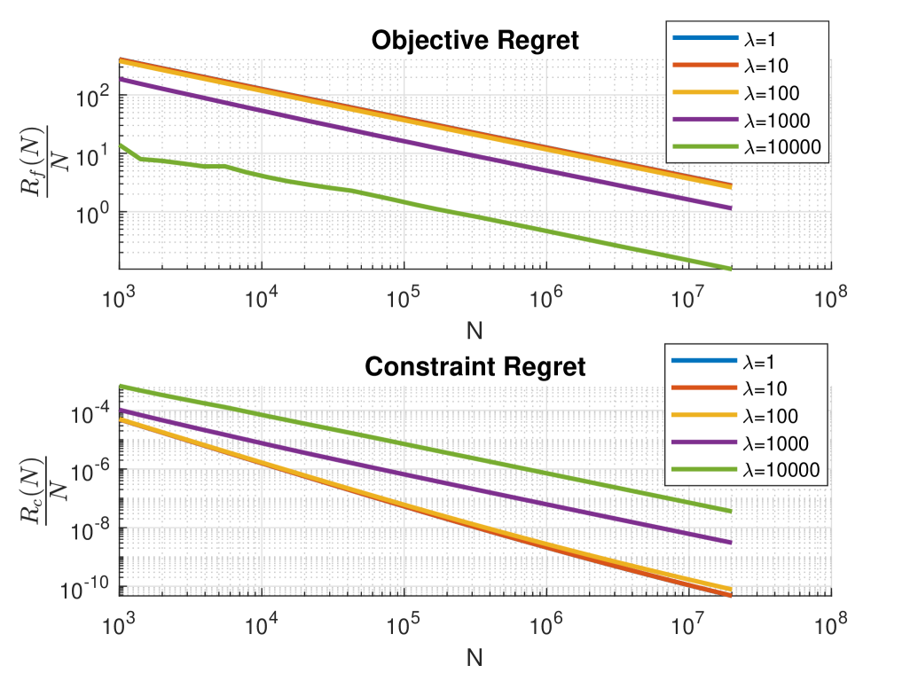
Figure 1: Objective and constraint regret for online LASSO.

5.2 Online learning of a static model

Consider the dataset generated by the static nonlinear model

$$y^{m}_{k}=\frac{z_{1,k}^{2}-e^{\frac{z_{2,k}}{10}}}{3+|z_{1,k}+z_{2,k}|}+r_{k}.$$

We want to train online a neural network $h_{k}(x)$ with $2$ layers, $8$ neurons in each layer, and $\tanh$ activation function, with $n_{x}=105$ trainable weights in total. The training is performed on $N=10^{5}$ randomly generated data points. Let $\{x_{k}\}_{k=0}^{N-1}$ be the sequence of weights generated by Algorithm 1. We evaluate the performance by means of the regret function $R_{f}(N)=\sum_{k=0}^{N-1}(f_{k}(x_{k})+g(x_{k}))-\min_{x}\sum_{k=0}^{N-1}(f_{k}(x)+g(x))$, where $f_{k}(x)=\frac{1}{2}\left\lVert y_{k}^{m}-h_{k}(x)\right\rVert^{2}$ and the optimal solution in hindsight is computed by performing 150 epochs using the NAILM algorithm proposed in [23]. The following performance indices will be used for evaluating the quality of the current solution $x$:

$$\begin{array}[]{rl}\text{Loss}(x)&=\frac{1}{N}\sum_{k=0}^{N-1}(f_{k}(x)+g(x))\\ \text{Mse}(x)&=\frac{1}{N}\sum_{k=0}^{N-1}f_{k}(x)\\ \text{Reg}(x)&=\frac{1}{N}\sum_{k=0}^{N-1}g(x)\\ \text{Cv}(x)&=\left\lVert x-\Pi_{\mathcal{C}}(x)\right\rVert_{2}^{2}\end{array}$$

where $\Pi_{\mathcal{C}}(x)$ is the projection of the point $x$ onto the set $\mathcal{C}$. The training is performed in MATLAB R2022a on an Intel Core i7 12700H CPU with 16 GB of RAM, using the library CasADi [24] to compute the required Jacobian matrices via automatic differentiation. All results are averaged over 20 runs starting from different initial conditions, that were randomly generated using Xavier initialization [25].

5.2.1 $\ell_{1}$ regularization

We train the neural model under the regularization function $g(x)=\lambda\left\lVert x\right\rVert_{1}$, with $\lambda=10^{-4}$. We selected the following hyper-parameters: $\rho=10\lambda$, $n_{a}=1$, $Q_{k}=10^{-4}I$, $R_{k}=I$ and $P_{0|0}=100I$. We compare the results to different online optimization alternatives: online ADMM [7] with constant matrix $P=10^{-2}I$ (online-ADMM), EKF-ADMM with time-varying $\rho_{k}=10^{\frac{k}{N}-2}\lambda$ (EKF-ADMMtv), and EKF with $\ell_{1}$-regularization [23] (EKF-$\ell_{1}$). The reason for choosing a time-varying $\rho_{k}$ is that fake measurements are usually not accurate initially, so that it is better to start with a higher value of $\frac{1}{\rho_{k}}$ and then decrease it progressively. In addition, we compare with two offline batch algorithms: NAILM [23] and LBFGS [26], the latter using the Python library jax-sysid. Such batch approaches are considered just for performance comparison. The results obtained at the end of the training phase are averaged over $20$ runs and reported in Table 1.

Table 1: Online learning a static model of (1) with $\ell_{1}$ regularization: mean Loss, Mse, sparsity ratio and execution time (standard deviation) obtained over 20 runs.

	Loss ($10^{-3}$)	Mse ($10^{-3}$)	Sparsity (%)	Time [s]
LBFGS [26]	$5.40$ ($0.72$)	$1.03$ ($0.19$)	$80.66$ ($5.32$)	$80.51$ ($2.42$)
NAILM [23]	$5.24$ ($0.48$)	$1.06$ ($0.15$)	$63.85$ ($5.00$)	$235.41$ ($52.78$)
EKF-ADMM	$5.99$ ($0.68$)	$1.44$ ($0.17$)	$45.28$ ($4.98$)	$58.27$ ($1.41$)
EKF-ADMMtv	$5.27$ ($0.46$)	$1.29$ ($0.42$)	$57.00$ ($7.95$)	$55.90$ ($1.41$)
online-ADMM [7]	$10.38$ ($1.7$)	$4.68$ ($1.8$)	$3.62$ ($2.21$)	$530.69$ ($29.09$)
EKF-$\ell_{1}$ [23]	$5.47$ ($0.67$)	$1.42$ ($0.26$)	$56.42$ ($7.67$)	$12.46$ ($0.27$)

EKF-ADMMtv provides the lowest loss. This is also true during the training phase, as shown in Figure 2. Note that all the online algorithms consume the dataset only once (1 epoch), except NAILM and LBFGS that run over 150 and 5000 epochs respectively. The slow execution of online-ADMM is due to solving a non-convex optimization problem at each time step, that we solved using the MATLAB function fminunc (quasi-Newton optimizer). LBFGS provides very sparse solutions, even at the cost of a slightly higher loss function, suggesting that it is particularly suited for sparsification. The online learning performance of EKF-ADMM can be also evaluated by looking at the regret function in Figure 3, where it is also apparent that the proposed algorithm improves the solution quality as more samples are provided.

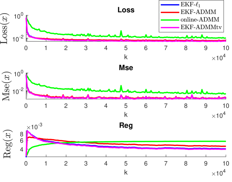
Figure 2: Online learning with $\ell_{1}$ regularization: Loss, Mse and Reg averaged over $20$ runs.

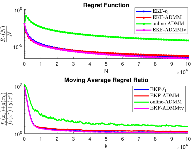
Figure 3: Online learning with $\ell_{1}$ regularization: regret and sample regret averaged over $20$ runs.

5.2.2 Bound constraints

Let us now repeat the training under the bound constraints imposed by the regularization function $g(x)=0$ if $x\in\mathcal{C}$ and $g(x)=+\infty$ otherwise, where $\mathcal{C}=\{x\in\mathbb{R}^{n_{x}}:\ |x_{i}|\leq 0.5\}$. We use the hyper-parameters $\rho=1,n_{a}=5,Q_{k}=10^{-4}I,P_{0|0}=100I$, and $R_{k}=I$. In this example, besides the batch solution obtained by running NAILM, we also run a simple clipping step of the Kalman filter (EKF-CLIP), to compare our proposed approach with a naive solution. Results obtained at the end of the training phase and averaged over $20$ runs are reported in Table 2. EKF-ADMM better enforces constraints that EKF-CLIP. Figure 2 shows the performance of the solution during the training phase. Among the online approaches, considering the final Mse, Cv and execution time, EKF-ADMM provides the best quality solution.

Table 2: Online learning a static model (1) with bound constraints: mean (standard deviation) Mse, constraints violation, and execution time averaged over 20 runs.

	Mse	Cv ($10^{-6}$)	Time [s]
LBFGS [26]	$0.122$ ($0.011$)	$0$ ($0$)	$75.87$ ($5.58$)
NAILM [23]	$0.137$ ($0.013$)	$0.38$ ($0.71$)	$101.82$ ($3.88$)
EKF-ADMM	$0.131$ ($0.011$)	$10.76$ ($4.93$)	$70.46$ ($3.45$)
online-ADMM [7]	$0.129$ ($0.010$)	$90.77$ ($59.37$)	$610.73$ ($9.82$)
EKF-CLIP	$0.214$ ($0.048$)	$0$ ($0$)	$11.89$ ($0.12$)

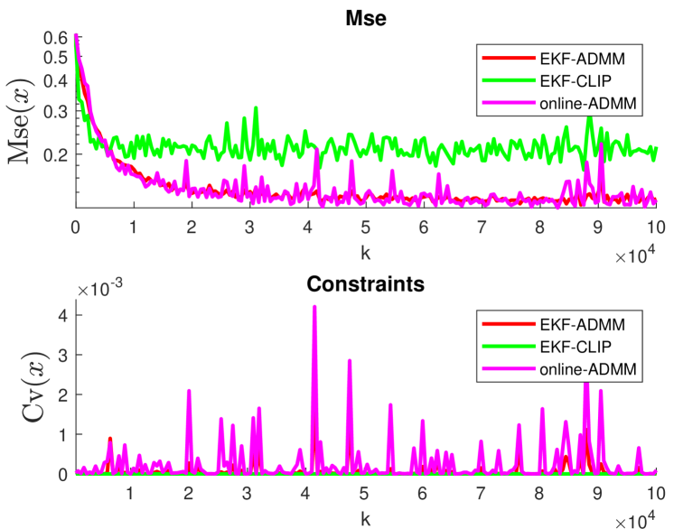
Figure 4: Online learning with bounds: Mse and constraints violation averaged over 20 runs.

5.3 Online learning of a time-varying model

We test now the ability of EKF-ADMM to adapt the same neural network model, under $\ell_{0}$ regularization, when the data-generating system switches as follows:

$$y^{m}_{k}=\begin{cases}\frac{z_{1,k}^{2}-e^{\frac{z_{2,k}}{10}}}{3+|z_{1,k}+z_{2,k}|}+r_{k}\;\;k\leq\frac{N}{3}\\ \frac{z_{1,k}^{2}-e^{\frac{z_{2,k}}{2}}}{3+|z_{1,k}+z_{2,k}|}+r_{k}\;\;\frac{N}{3}<k\leq\frac{2N}{3}\\ \frac{0.3\cdot z_{1,k}^{2}-e^{\frac{z_{2,k}}{2}}}{3+|z_{1,k}+z_{2,k}|}+r_{k}\;\;\frac{2N}{3}<k\\ \end{cases}$$ (13)

with $N=1.5\cdot 10^{5}$. We evaluate the regret function $R_{f}(N)=\sum_{k=0}^{N-1}(f_{k}(x_{k})+g(x_{k}))-\min_{z_{1},z_{2},z_{3}}\sum_{i=1}^{3}r_{i}(z_{i})$, with $r_{i}(z_{i})=\sum_{k=(i-1)\frac{N}{3}}^{i\frac{N}{3}}(f_{k}(z_{i})+g(z_{i}))$, where $\{x_{k}\}_{k=0}^{N-1}$ is the sequence generated by Algorithm 1. The regularization term is $g(x)=\lambda\left\lVert w\right\rVert_{0}$, with $\lambda=10^{-4}$, and use the EKF-ADMM hyper-parameters $\rho=10^{3}\cdot\lambda$, $p_{a}=1$, $Q_{k}=10^{-4}I$, and $P_{0|0}=100I$. Since the model is now time-varying, we will also use an EKF implementation with forgetting factor $\alpha=0.9$ [12], which simply amounts of scaling the covariance matrix as $\frac{1}{\alpha}P_{k}$ at each step. The resulting regret function is shown in Figure 5. It is apparent that EKF-ADMM can track changes of the underlying data-generating system.

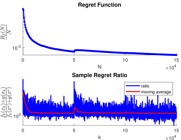
Figure 5: Online learning with $\ell_{0}$ regularization: regret and sample regret averaged over $20$ runs.

6 Conclusions

We have proposed a novel algorithm for online learning of nonlinear parametric models under non-smooth regularization using a combination of EKF and ADMM, for which we derived a sublinear regret bound for the convex linear time-varying case. The approach is computationally cheap and is suitable for factorized or square-root implementations that can make it numerically robust, and is therefore very appealing for embedded applications of adaptive control, such as adaptive model predictive control. The effectiveness of the approach has been evaluated in three numerical examples. Future investigations will focus on extending the approach to the recursive identification of parametric nonlinear state-space dynamical models from input/output data under non-smooth regularization, in which both the hidden states and the parameters are jointly estimated.

Appendix A Proof of Theorem 1

Starting from $R_{f}(N)$, since $x_{k+1},\nu_{k+1}$ are the optimal solutions of the first two optimization problems in Algorithm 2 and since $w_{k}=w_{k+1}-\rho(x_{k+1}-\nu_{k+1})$ we have that $\nabla f_{k}(x_{k+1})=-(w_{k+1}-\rho(\nu_{k}-\nu_{k+1}))-\eta(P_{k}^{-1}x_{k+1}-P_{k}^{-1}x_{k})$ and $w_{k+1}\in\partial g(\nu_{k+1})$, where $\partial g$ is the subgradient of $g$. Due to the convexity of $f_{k}(\cdot)$ and $g(\cdot)$,

$$f_{k}(x_{k+1})-f_{k}(x^{\star})\leq\nabla f_{k}(x_{k+1})^{T}(x_{k+1}-x^{\star})=-w_{k+1}^{T}(x_{k+1}-\nu^{\star})+\frac{\rho}{2}(\left\lVert\nu^{\star}-\nu_{k}\right\rVert^{2}-\left\lVert\nu^{\star}-\nu_{k+1}\right\rVert^{2}+$$ (14)

$$\left\lVert x_{k+1}-\nu_{k+1}\right\rVert^{2}-\left\lVert x_{k+1}-\nu_{k}\right\rVert^{2})+\frac{\eta}{2}\left(\left\lVert x^{\star}-x_{k}\right\rVert^{2}_{P_{k}^{-1}}-\left\lVert x^{\star}-x_{k+1}\right\rVert^{2}_{P_{k}^{-1}}-\left\lVert x_{k+1}-x_{k}\right\rVert^{2}_{P_{k}^{-1}}\right)$$

and

$$g(\nu_{k+1})-g(\nu^{\star}) \leq w_{k+1}^{T}(\nu_{k+1}-\nu^{\star})$$ (15)

Summing Eqs. (14)-(15) together and noticing that $-w_{k+1}^{T}(x_{k+1}-\nu_{k+1})+\frac{\rho}{2}(x_{k+1}-\nu_{k+1})=\frac{1}{2\rho}(\left\lVert w_{k}\right\rVert^{2}-\left\lVert w_{k+1}\right\rVert^{2})$, we obtain:

$$f_{k}(x_{k+1})+g(\nu_{k+1})-(f_{k}(x^{\star})+g(\nu^{\star}))\leq\frac{1}{2\rho}(\left\lVert w_{k}\right\rVert^{2}-\left\lVert w_{k+1}\right\rVert^{2})-\frac{\rho}{2}\left\lVert x_{k+1}-\nu_{k}\right\rVert^{2}+$$ (16)

$$\frac{\rho}{2}(\left\lVert\nu^{\star}-\nu_{k}\right\rVert^{2}-\left\lVert\nu^{\star}-\nu_{k+1}\right\rVert^{2})+\frac{\eta}{2}(\left\lVert x^{\star}-x_{k}\right\rVert^{2}_{P_{k}^{-1}}-\left\lVert x^{\star}-x_{k+1}\right\rVert^{2}_{P_{k}^{-1}}-\left\lVert x_{k+1}-x_{k}\right\rVert^{2}_{P_{k}^{-1}})$$

Considering that $f_{k}(x_{k})-f_{k}(x_{k+1})\leq\nabla f_{k}(x_{k})^{T}(x_{k}-x_{k+1})\leq\frac{1}{2\alpha\eta}\left\lVert\nabla f_{k}(x_{k})\right\rVert^{2}+\frac{\alpha\eta}{2}\left\lVert x_{k}-x_{k+1}\right\rVert^{2}$, where the second inequality is due to Fenchel-Young’s inequality, and considering Assumption A1.a of the theorem, we have that:

$$f_{k}(x_{k})+g(\nu_{k+1})-(f_{k}(x^{\star})+g(\nu^{\star}))\leq\frac{1}{2\rho}(\left\lVert w_{k}\right\rVert^{2}-\left\lVert w_{k+1}\right\rVert^{2})-\frac{\rho}{2}\left\lVert x_{k+1}-\nu_{k}\right\rVert^{2}+\frac{\rho}{2}(\left\lVert\nu^{\star}-\nu_{k}\right\rVert^{2}$$

$$\left.-\left\lVert\nu^{\star}-\nu_{k+1}\right\rVert^{2}\right)+\frac{1}{2\alpha\eta}\left\lVert\nabla f_{k}(x_{k})\right\rVert^{2}+\frac{\eta}{2}(\left\lVert x^{\star}-x_{k}\right\rVert_{P_{k}^{-1}}^{2}-\left\lVert x^{\star}-x_{k+1}\right\rVert_{P_{k}^{-1}}^{2}).$$

Summing from 0 to $N-1$ and considering Assumption A3 we get

$$R_{f}(N)=\sum_{k=0}^{N-1}(f_{k}(x_{k})+g(\nu_{k+1})-(f_{k}(x^{\star})+g(\nu^{\star})))+g(\nu_{0})-g(\nu_{N})\leq$$

$$\leq\frac{1}{2\rho}(\left\lVert w_{0}\right\rVert^{2}-\left\lVert w_{N}\right\rVert^{2})+\frac{\rho}{2}(\left\lVert\nu^{\star}-\nu_{0}\right\rVert^{2}-\left\lVert\nu^{\star}-\nu_{N}\right\rVert^{2})+\frac{1}{2\alpha\eta}\sum_{k=0}^{N-1}\left\lVert\nabla f_{k}(x_{k})\right\rVert^{2}+\frac{\eta}{2}\left\lVert x^{\star}-x_{0}\right\rVert^{2}_{P_{0}^{-1}}$$

$$+\frac{\eta}{2}\sum_{k=1}^{N-1}\left\lVert x^{\star}-x_{k}\right\rVert^{2}_{(P_{k}^{-1}-P_{k-1}^{-1})}$$

and, therefore, $R_{f}(N)\leq\frac{\rho}{2}\left\lVert\nu^{\star}\right\rVert^{2}$ $+\frac{1}{2\alpha\eta}\sum_{k=0}^{N-1}\left\lVert\nabla f_{k}(x_{k})\right\rVert^{2}+\frac{\eta}{2}\left\lVert x^{\star}\right\rVert^{2}_{P_{0}^{-1}}+\frac{\eta}{2}\sum_{k=1}^{N-1}\left\lVert x^{\star}-x_{k}\right\rVert^{2}_{(P_{k}^{-1}-P_{k-1}^{-1})}$. Because of Assumption A2, $\frac{1}{2}\sum_{k=1}^{N-1}\left\lVert x^{\star}-x_{k}\right\rVert^{2}_{(P_{k}^{-1}-P_{k-1}^{-1})}=\frac{1}{2}\sum_{k=1}^{k_{n}}\left\lVert x^{\star}-x_{k}\right\rVert^{2}_{(P_{k}^{-1}-P_{k-1}^{-1})}\leq M_{k_{n}}$, and taking into account Assumptions A1.b and A1.c we get $R_{f}(N)\leq\frac{\rho D_{\nu}}{2}+\frac{NG_{f}^{2}}{2\alpha\eta}+\eta(D_{x}^{2}+M_{k_{n}})$. Setting $\eta\stackrel{{\scriptstyle\text{def}}}{{=}}\frac{G_{f}\sqrt{N}}{D_{x}\sqrt{2\alpha}}$ and $\rho\stackrel{{\scriptstyle\text{def}}}{{=}}\sqrt{N}$, we get the sublinear regret bound $R_{f}(N)\leq\frac{\sqrt{N}D_{\nu}}{2}+\frac{G_{f}D_{x}\sqrt{N}}{\sqrt{2\alpha}}+\frac{G_{f}\sqrt{N}(D_{x}^{2}+M_{k_{n}})}{D_{x}\sqrt{2\alpha}}$. Considering now $R_{c}(N)$, we can rearrange (16) and consider Assumption A1.d:

$$\left\lVert x_{k+1}-\nu_{k}\right\rVert^{2}\leq\frac{2F}{\rho}+\frac{1}{\rho^{2}}(\left\lVert w_{k}\right\rVert^{2}-\left\lVert w_{k+1}\right\rVert^{2})+(\left\lVert\nu^{\star}-\nu_{k}\right\rVert^{2}-\left\lVert\nu^{\star}-\nu_{k+1}\right\rVert^{2})+\frac{\eta}{\rho}(\left\lVert x^{\star}-x_{k}\right\rVert_{P_{k}^{-1}}^{2}$$

$$-\left\lVert x^{\star}-x_{k+1}\right\rVert_{P_{k}^{-1}}^{2}-\left\lVert x_{k+1}-x_{k}\right\rVert_{P_{k}^{-1}}^{2}).$$

Summing from 0 to $N-1$, we get:

$$R_{c}(N)=\sum_{k=0}^{N-1}\left\lVert x_{k+1}-\nu_{k}\right\rVert^{2}\leq\frac{2FN}{\rho}+\left\lVert\nu^{\star}\right\rVert^{2}+\frac{\eta}{\rho}\bigg{(}\left\lVert x^{\star}\right\rVert^{2}_{P_{0}^{-1}}+\sum_{k=1}^{N-1}\left\lVert x^{\star}-x_{k}\right\rVert^{2}_{(P_{k}^{-1}-P_{k-1}^{-1})}\bigg{)}.$$

Considering Assumptions A1.c and A2, we have $R_{c}(N)\leq\frac{2FN}{\rho}+D_{\nu}+\frac{2\eta}{\rho}(D_{x}^{2}+M_{k_{n}})$ and setting $\eta\stackrel{{\scriptstyle\text{def}}}{{=}}\frac{G_{f}\sqrt{N}}{D_{x}\sqrt{2\alpha}}$ and $\rho\stackrel{{\scriptstyle\text{def}}}{{=}}\sqrt{N}$ we finally get $R_{c}(N)\leq 2F\sqrt{N}+D_{\nu}+\frac{2G_{f}}{D_{x}\sqrt{2\alpha}}(D_{x}^{2}+M_{k_{n}})$. $\Box$

References

- [1] J. Schoukens and L. Ljung. Nonlinear system identification: A user-oriented road map. IEEE Control Systems, 39:28–99, 2019.
- [2] G. Pillonetto, A. Aravkin, D. Gedon, L. Ljung, A. H. Ribeiro, and T. B. Schön. Deep networks for system identification: A survey. Automatica, 171:111907, 2025.
- [3] C. Louizos, M. Welling, and D. P. Kingma. Learning sparse neural networks through regularization. In International Conference on Learning Representations, 2018.
- [4] S.C.H. Hoi, D. Sahoo, J. Lu, and P. Zhao. Online learning: A comprehensive survey. Neurocomputing, 459:249–289, 2021.
- [5] H. Robbins and S. Monro. A stochastic approximation method. The annals of mathematical statistics, 22(3):400–407, 1951.
- [6] H.B. McMahan. Follow-the-regularized-leader and mirror descent: Equivalence theorems and L1 regularization. In Proc. 14th Int. Conference on Artificial Intelligence and Statistics, 2011.
- [7] H. Wang and A. Banjaree. Online alternating direction method. In Proc. 29th International Conference on Machine Learning, pages 1699–1706, Edinburgh, Scotland, UK, 2012.
- [8] S. Singhal and L. Wu. Training feed-forward networks with the extended Kalman algorithm. In International Conference on Acoustics, Speech, and Signal Processing,, pages 1187–1190, 1989.
- [9] G.V. Puskorius and L.A. Feldkamp. Neurocontrol of nonlinear dynamical systems with Kalman filter trained recurrent networks. IEEE Transactions on Neural Networks, 5(2):279–297, 1994.
- [10] R.J. Williams. Training recurrent networks using the extended Kalman filter. In IJCNN Int. Joint Conf. on Neural Networks, volume 4, pages 241–246, 1992.
- [11] A. Bemporad. Recurrent neural network training with convex loss and regularization functions by extended kalman filtering. IEEE Transactions on Automatic Control, 68(1):5661–5668, 2021.
- [12] A. Abulikemu and L. Changliu. Robust online model adaptation by extended Kalman filter with exponential moving average and dynamic multi-epoch strategy. In Proc. 2nd Conference on Learning for Dynamics and Control, volume 120, pages 65–74, 2020.
- [13] H.J. Sena, F.V. da Silva, and A.M.F. Fileti. ANN model adaptation algorithm based on extended Kalman filter applied to pH control using MPC. Journal of Process Control, 102:15–23, 2021.
- [14] T.K. Chang, D.L. Yu, and D.W. Yu. Neural network model adaptation and its application to process control. Advanced Engineering Informatics, 18(1):1–8, 2004.
- [15] R.E. Kalman. A new approach to linear filtering and prediction problems. ASME. J. Basic Eng, 82(1):35–45, 1960.
- [16] H. Jeffrey, R. Preston, and W. Jeremy. A fresh look at the Kalman filter. SIAM Review, 54(4):801–823, 2012.
- [17] S. Boyd, N. Parikh, E. Chu, B. Peleato, and J. Eckstein. Distributed optimization and statistical learning via the alternating direction method of multipliers. Foundations and Trends in Machine Learning, 3(1):1–122, 2011.
- [18] N. Parikh and S. Boyd. Proximal algorithms. Foundations and Trends in Optimization, 1(3):123–231, 2013.
- [19] C.L. Thornton and G.J. Bierman. Gram-Schmidt algorithms for covariance propagation. In IEEE Conference on Decision and Control, pages 489–498, 1975.
- [20] G.J. Bierman. Measurement updating using the U-D factorization. Automatica, 12(4):375–382, 1976.
- [21] Y. Zhang, Z. Xiao, J. Wu, and L. Zhang. Online alternating direction method of multipliers for online composite optimization. arXiv preprint arXiv:1904.02862, 2024.
- [22] J. Ranstam and J.A. Cook. LASSO regression. British Journal of Surgery, 105(10):1348–1348, 2018.
- [23] A. Bemporad. Training recurrent neural networks by sequential least squares and the alternating direction method of multiplier. Automatica, 156(1):111183, 2023.
- [24] J.A.E. Andersson, J. Gillis, G. Horn, J.B. Rawlings, and M. Diehl. CasADi – A software framework for nonlinear optimization and optimal control. Mathematical Programming Computation, 11(1):1–36, 2019.
- [25] X. Glorot and Y. Bengio. Understanding the difficulty of training deep feedforward neural networks. In Proc. 13 Int. Conf. Artificial Intelligence and Statistics, pages 249–256, 2010.
- [26] A. Bemporad. An L-BFGS-B approach for linear and nonlinear system identification under and group-lasso regularization. IEEE Transactions on Automatic Control, 2025. in press.