A hierarchical approach for multicontinuum homogenization in high contrast media

Abstract

A recently developed upscaling technique, the multicontinuum homogenization method, has gained significant attention for its effectiveness in modeling complex multiscale systems. This method defines multiple continua based on distinct physical properties and solves a series of constrained cell problems to capture localized information for each continuum. However, solving all these cell problems on very fine grids at every macroscopic point is computationally expensive, which is a common limitation of most homogenization approaches for non-periodic problems. To address this challenge, we propose a hierarchical multicontinuum homogenization framework. The core idea is to define hierarchical macroscopic points and solve the constrained problems on grids of varying resolutions. We assume that the local solutions can be represented as a combination of a linear interpolation of local solutions from preceding levels and an additional correction term. This combination is substituted into the original constrained problems, and the correction term is resolved using finite element (FE) grids of varying sizes, depending on the level of the macropoint. By normalizing the computational cost of fully resolving the local problem to $\mathcal{O}(1)$, we establish that our approach incurs a cost of $\mathcal{O}(L\eta^{(1-L)d})$, highlighting substantial computational savings across hierarchical layers $L$, coarsening factor $\eta$, and spatial dimension $d$. Numerical experiments validate the effectiveness of the proposed method in media with slowly varying properties, underscoring its potential for efficient multiscale modeling.

Keywords: Hierarchical, upscaling method, multicontinuum, homogenization

1 Introduction

Multiscale phenomena are common in engineering and industrial applications, involving processes that interact across different scales. For example, in fluid flow through porous media, features like fractures, vugs, and micropores are crucial for determining properties such as permeability and fluid transport, which are critical to subsurface flow modeling and material design. In composite materials, the arrangement of fibers and matrix influences heat conduction, affecting the thermal behavior of engineering materials. Similarly, in electromagnetic wave propagation, the structure of materials like layered composites or metamaterials affects the dispersion and absorption of waves. However, traditional numerical methods, such as the finite element method and the finite volume method, often have difficulty resolving the fine-scale details of these multiscale materials due to high computational costs and complexity. Developing an efficient multiscale method is therefore necessary.

Among the various approaches developed for multiscale problems, an important class focuses on constructing local basis functions on fine grids and solving the resulting algebraic systems on coarse grids. This approach balances computational efficiency with the preservation of fine-scale details. Key methods in this category include the localized orthogonal decomposition method [23, 17], which generates localized multiscale basis functions through systematic decomposition of solution spaces, effectively capturing fine-scale information while reducing computational cost. The multiscale finite element method (MsFEM) [21, 20, 30, 22] employs precomputed basis functions to account for fine-scale heterogeneities, enabling accurate coarse-scale simulations. The generalized multiscale finite element method (GMsFEM) [13, 6, 2, 27, 11, 31, 16] extends the multiscale finite element method (MsFEM) by introducing symmetric and adaptive basis function construction. The constraint energy minimizing generalized multiscale finite element method (CEM-GMsFEM) [8, 29, 25, 28] further constructs local basis functions by solving energy minimization problems within oversampled domains.

In contrast, some problems necessitate a focus solely on macroscopic variables, circumventing the need to resolve fine-scale details explicitly. Upscaling techniques establish a connection between microscopic and macroscopic scales by assuming that microscale solutions can be represented using different ansatzes of the macroscale solutions. Examples include homogenization [19, 12] and the heterogeneous multiscale method [1, 18]. In this paper, we focus on the multicontinuum homogenization method [7, 14, 26, 15, 3]. This method defines multiple continua to represent distinct physical regions. The macroscopic coefficient is obtained by solving a series of constraint problems in an oversampled representative volume element (or target coarse block) region. The constraints in the cell problems are used to represent different behaviors for different continua, which has been widely investigated in nonlocal multicontinuum upscaling (NLMC) methods [10, 9], as well as in the CEM-GMsFEM [8]. In fact, the accuracy of the upscaling coefficient depends heavily on the finite element (FE) grid used to solve the cell problems. In practice, since local geometries or material properties are typically non-periodic, resolving all cell problems on very fine grids is computationally expensive. For this reason, we introduce a general framework to hierarchically compute the upscaling coefficient.

In this work, we propose a general framework for hierarchical multicontinuum homogenization. Our approach mainly consists of three steps: First, we divide the macropoints (the centers of the coarse blocks) into a hierarchical grid, similar to previous works [24, 4, 5]. Then, we define the FE spaces for different levels. Finally, we construct the local solutions inductively for different levels. We assume that the local solutions can be expressed as a combination of the linear interpolation of local solutions from other macropoints at preceding levels and an additional correction term. After substituting this combination into the original constraint problem, we obtain a constraint problem for the correction term. In this way, the computational cost mainly stems from numerically solving the correction term. By using the nested FE spaces we define, the computational cost can be reduced compared to using the same fine FE grid for each macropoint. We also discuss the detailed computational cost of the original multicontinuum homogenization method and the hierarchical multicontinuum homogenization method. In addition, we design four numerical examples to test the performance of our method. We compute three types of errors: (1) the error from the original multicontinuum homogenization method, (2) the error of the hierarchical multicontinuum homogenization method, and (3) the error of the hierarchical part. Our numerical results show that if the physical properties do not vary drastically, our approach achieves high accuracy. Even when the physical regions have dramatic variations, it can still provide acceptable accuracy.

This paper is organized as follows. In Section 2, we present the model problem and review the multicontinuum homogenization method. In Section 3, we detail the hierarchical computation of the upscaling coefficient and discuss the computational savings. The numerical results are presented in Section 4. Finally, the paper concludes with a summary in Section 5.

2 Preliminaries

In this section, we present the model problem and review the multicontinuum homogenization framework introduced in [14, 7]. Let $\Omega\subset\mathbb{R}^{d}$ ($d=2,3$) be a convex region. We consider the following equation:

$$\mathcal{A}^{\epsilon}u=f\quad\textnormal{in}~\Omega,$$ (1)

where $\mathcal{A}^{\epsilon}$ is a linear differential operator, and $u$ vanishes on the boundary. For simplicity, we consider the scalar elliptic equation: $\mathcal{A}^{\epsilon}(u)=-\nabla\cdot(\kappa\nabla u)$. The weak formulation of Eq. (1) is

$$\int_{\Omega}\kappa\nabla u\nabla v=\int_{\Omega}fv,\quad\forall v\in V,$$ (2)

where $V$ is $H_{0}^{1}(\Omega)$. In this paper, we use $h$ to represent the mesh size that can resolve the heterogeneities caused by the coefficients or geometries and achieve high accuracy. To avoid the unaffordable algebra system from that mesh size, we use the multicontinuum homogenization method to build an upscaling model and solve it at the macroscopic scale.

Figure 1: Illustration of RVE $R_{p}$, oversampling domain $R_{p}^{+}$ and coarse block $K_{p}$.

We present the computational grid for multicontinuum homogenization. In Figure 1, the computation domain $\Omega$ is divided into a series of coarse blocks. We select a coarse block $K_{p}$, whose center is $x_{p}^{*}$. In the rest of this paper, the superscript $*$ is used to denote the macropoint. The representative volume element (RVE) $R_{p}$ is used to capture the local heterogeneity information at the macropoint $x_{p}^{*}$. To reduce the influence of artificial boundary conditions, we apply oversampling to $R_{p}$ to get $R_{p}^{+}$.

The continuum is defined through different characteristic functions $\psi_{i}^{p}$ in the corresponding representative volume element $R_{p}$. Specifically, $\psi_{i}^{p}=1$ in continuum $i$ and $0$ elsewhere. We use two continua for illustration, but this approach can be extended to multiple continua. We then assume that the unknown variable $u$ can be expanded as a series of products of macroscopic variables $U_{i}$ and local microscopic functions $\phi$’s:

$$u=\phi_{i}U_{i}+\phi_{i}^{m}\partial_{m}U_{i}+\phi_{i}^{mn}\partial_{mn}^{2}U_{i}+\cdots\quad\textnormal{in}~R_{p},$$

where $\partial_{m}=\frac{\partial}{\partial x_{m}}$ and $\partial_{mn}^{2}=\frac{\partial^{2}}{\partial x_{m}\partial x_{n}}$. We adopt the Einstein summation convention for simplicity, for example:

$$\phi_{i}U_{i}=\sum_{i=1}^{2}\phi_{i}U_{i},~\phi_{i}^{m}\partial_{m}U_{i}=\sum_{i=1}^{2}\sum_{m=1}^{d}\phi_{i}^{m}\partial_{m}U_{i},$$

unless otherwise stated, in which case the summation sign will be omitted. The macroscopic function $U_{i}$ is smooth and defined on the computational domain $\Omega$. Its value at the center $x_{p}^{*}$ is given by $U_{i}(x_{p}^{*})=\int_{R_{p}}\psi_{i}u/\int_{R_{p}}\psi_{i}$.

In general, we only consider the constant and linear behavior of macroscopic functions. That is, we assume $u\approx\phi_{i}U_{i}+\phi_{i}^{m}\partial_{m}U_{i}$. The local solutions $\phi$ are constructed by numerically solving a constrained problem in an oversampled domain $R_{p}^{+}$. The first-type saddle point problem is formulated by imposing constraints designed to capture the macroscopic average behavior of multiple continua.

$$\int_{R_{p}^{+}}\kappa\nabla\phi_{i}\cdot v-\sum_{j,q}\frac{\beta_{ij}^{q}}{\int_{R_{q}}\psi_{j}}\int_{R_{q}}\psi_{j}v=0,$$ (3)

$$\int_{R_{q}}\phi_{i}\psi_{j}=\delta_{ij}\int_{R_{q}}\psi_{j},\quad\forall R_{q}\in R_{p}^{+}.$$

The second-type saddle point problem imposes constraints to represent the macroscopic linear behavior of each continuum.

$$\int_{R_{p}^{+}}\kappa\nabla\phi_{i}\cdot v-\sum_{j,q}\frac{\beta_{ij}^{q}}{\int_{R_{q}}\psi_{j}}\int_{R_{q}}\psi_{j}v=0,$$ (4)

$$\int_{R_{q}}\phi_{i}^{m}\psi_{j}=\delta_{ij}\int_{R_{q}}(x_{m}-c_{mj})\psi_{j},\quad\forall R_{q}\in R_{p}^{+},$$

where $c_{mj}$ statisfy $\int_{K_{p}}(x_{m}-c_{mj})\psi_{j}^{p}=0.$ In Eqs. (3) and (4), $\beta$ denotes the Lagrange multiplier associated with the specified constraints. We assume the macroscopic function $U_{i}$ are smooth in the RVE, the variation is small compare to the local functions $\phi$. We have

$$\int_{R_{p}}\kappa\nabla(\phi_{i}U_{i})\nabla v\approx U_{i}(x_{p}^{*})\int_{R_{p}}\kappa\nabla\phi_{i}\nabla v,\quad\int_{R_{p}}\kappa\nabla(\phi_{i}^{m}\nabla_{m}U_{i})\nabla v\approx\nabla_{m}U_{i}(x_{p}^{*})\int_{R_{p}}\kappa\nabla\phi_{i}^{m}\nabla v.$$ (5)

Based on the approximation (5) and setting $v\approx\phi_{j}V_{j}+\phi_{j}^{n}\partial_{n}V_{j}$ in Eq. (2), we have the following result:

$$U_{i}V_{j}\sum_{p}\frac{|K_{p}|}{|R_{p}|}\int_{R_{p}}\kappa\nabla\phi_{i}\nabla\phi_{j}+V_{j}\nabla_{m}U_{i}\sum_{p}\frac{|K_{p}|}{|R_{p}|}\int_{R_{p}}\kappa\nabla\phi_{i}^{m}\nabla\phi_{j}+U_{i}\nabla_{n}V_{j}\sum_{p}\frac{|K_{p}|}{|R_{p}|}\int_{R_{p}}\nabla\phi_{i}\nabla\phi_{j}^{n}$$

$$+\nabla_{m}U_{i}\nabla_{n}V_{j}\sum_{p}\frac{|K_{p}|}{|R_{p}|}\int_{R_{p}}\kappa\nabla\phi_{i}^{m}\nabla\phi_{j}^{n}=\sum_{p}\frac{|K_{p}|}{|R_{p}|}\int_{R_{p}}f\phi_{j},$$

where $U_{i}$, $V_{j}$, and their gradients are taken at specific points, such as the midpoint of the coarse block. Moreover, the RVE index $p$ has been omitted here for simplicity, as it is independent across different macropoints. However, it will be explicitly included in the discussion of the hierarchical method.

Then, we obtain the following upscaling multicontinuum system in strong form:

$$B_{ji}U_{i}+B_{ji}^{m}\partial_{m}U_{i}-\partial_{n}\overline{B}_{ji}^{n}U_{i}-\partial_{n}(B_{ji}^{mn}\partial_{m}U_{i})=b_{j},$$ (6)

where the coefficients are piecewise-constant vectors or matrices,

$$B_{ji}=\frac{|K_{p}|}{|R_{p}|}\int_{R_{p}}\kappa\nabla\phi_{i}\nabla\phi_{j},~B_{ji}^{m}=\frac{|K_{p}|}{|R_{p}|}\int_{R_{p}}\kappa\nabla\phi_{i}^{m}\nabla\phi_{j},$$ (7)

$$\overline{B}_{ji}^{n}=\frac{|K_{p}|}{|R_{p}|}\int_{R_{p}}\kappa\nabla\phi_{i}\nabla\phi_{j}^{n},~B_{ji}^{mn}=\frac{|K_{p}|}{|R_{p}|}\int_{R_{p}}\kappa\nabla\phi_{i}^{m}\nabla\phi_{j}^{n},~b_{j}=\frac{|K_{p}|}{|R_{p}|}\int_{R_{p}}f\phi_{j},$$

3 Hierarchical multicontinuum homogenization

The main goal of hierarchical multicontinuum homogenization is to use a different FE grid size to solve the cell problems, while ensuring that all of them achieve the finest grid accuracy. All of the local solutions can be summarized as the following abstract problem:

$$\Phi_{p}=\min_{v\in V(R_{p})}\mathcal{A}^{\epsilon}(v)\quad\textnormal{subject to some constraints.}$$ (8)

The constraints are detailed in Eqs. (3) and (4). Hereafter, $\Phi_{p}$ is used to represent the local solutions at macropoint $x_{p}^{*}$, regardless of the specific type of local solutions. Since solving the cell problems for every macroscopic point using a very fine mesh remains a huge challenge, we design a hierarchical multicontinuum homogenization method to overcome this difficulty. For a given macroscopic point $x_{p}^{*}$, we assume that the local solutions $\Phi_{p}$ can be expressed as

$$\Phi_{p}=\Xi_{p}+\mathcal{I}_{p}(\Phi).$$ (9)

Here, $\mathcal{I}_{p}$ is a linear interpolation operator at $x_{p}^{*}$ using the local solutions that have already been constructed, and $\Xi_{p}$ is a correction term solved using a different size of the fine grid mesh. The computational process of our algorithm involves three steps: First, we build a dense hierarchical macrogrid $\{\mathcal{S}_{n}\}_{n=1}^{L}$ for the macropoint set $\mathcal{T}$. Second, we define a nested FE space $\{V_{n}\}_{n=1}^{L}$ to matching the hierarchical macrogrid $\{\mathcal{S}_{n}\}_{n=1}^{L}$. Finally, we substitute Eq. (9) into the constraint problem (8) and solve for the correction term $\Xi_{p}$ within the corresponding FE space. The framework of our method is listed in Algorithm 1.

Algorithm 1 Hierarchical multicontinuum homogenization method.

0: Macropoint set $\mathcal{T}$, coarsing factor $\eta$, fine grid mesh size $h$, levels $L$.

1: Divide $\mathcal{T}$ into a dense hierarchy of macroscopic point sets $\{\mathcal{S}_{n}\}_{n=1}^{L}$.

2: Define a nested FE space $\{V_{n}\}_{n=1}^{L}$ matching the hierarchical macroscopic points $\{\mathcal{S}_{n}\}_{n=1}^{L}$.

3: for $1\leq n\leq L$ do

4:  for $x_{p}^{*}\in\mathcal{S}_{n}$ do

5:   Substitute the approximation (9) into (8) and solve the correction term $\Xi_{p}$ in $V_{n}$.

6:   Compute the upscaling coefficients in $x_{p}^{*}$ by (7).

7:  end for

8: end for

9: Solving the upscaled multicontinuum system (6).

9: Upscaled solutions $U_{i}$.

In the following, we focus on the details of hierarchically computing the local solutions.

3.1 Build hierarchy of macrogrids

A hierarchical macrogrid can help us judiciously decide the FE mesh size for cell problems at different macrogrid points. We first build a nested macroscopic grid (cf. [4, 24, 5]) for the macropoint set $\mathcal{T}$, denoted as

$$\mathcal{T}_{1}\subset\mathcal{T}_{2}\subset\cdots\subset\mathcal{T}_{L}=\mathcal{T}.$$

The grid is constructed inductively, starting with an initial mesh $\mathcal{T}_{1}$ of size $\eta^{L}H$. Here, $H$ denotes the original coarse mesh size, i.e., the coarse mesh size at the last level $\mathcal{T}_{L}$, and $\eta$ is the grid coarsening factor. At each subsequent step, the refinement $\mathcal{T}_{n}$ is obtained from the preceding grid $\mathcal{T}_{n-1}$, with the mesh size reduced to $\eta^{L-n}H$. For the given $n$-th level, we ensure that there is a macropoint in the coarse block with mesh size $\eta^{L-n}H$. To avoid repeated computations, we remove the overlapping macropoints to build the hierarchical macrogrids $\{\mathcal{S}_{n}\}_{n=1}^{L}$, that is,

$$\mathcal{S}_{n}=\mathcal{T}_{n}\big{\backslash}\left(\bigcup_{k<n}\mathcal{S}_{k}\right).$$ (10)

Specifically, for the first level, we define $\mathcal{S}_{1}=\mathcal{T}_{1}$. From (10), we can also obtain the following property: $\mathcal{S}_{n+1}=\mathcal{T}_{n+1}\backslash\mathcal{T}_{n}$. Constructed in this way, the macrogrids have the dense property. That is, for any macroscopic point $x_{p}^{*}\in\mathcal{S}_{n}$, there exists at least one point $x_{q}^{*}\in\bigcup_{k<n}~\mathcal{S}_{k}$ such that $\mathrm{dist}(x_{p}^{*},x_{q}^{*})<O(\eta^{L-n}H)$. This paves the way for our next nested FE space definition and also the linear interpolation operator.

Figure 2: 3-level nested macrogrids.

In Figures 2 and 3, we illustrate an example of three-level nested macrogrids $\{\mathcal{T}_{n}\}_{n=1}^{3}$ and the corresponding hierarchical structures $\{\mathcal{S}_{n}\}_{n=1}^{3}$ in a unit square. Here, the final coarse mesh size is $H=1/8$, and the coarsening factor is $\eta=2$. As the coarse mesh decreases from $4H$ to $2H$, and then to $H$, a macroscopic point remains within the corresponding coarse block in $\mathcal{T}_{n}$.

Figure 3: 3-level hierarchical macrogrids.

3.2 Build nested FE spaces

For a given macrogrid point $x_{p}^{*}\in\mathcal{S}_{n}$, we denote the corresponding FE space as $V_{n}$. More specifically, the FE space $V_{n}$ is defined on the FE grid with a mesh size of $h\eta^{n-1}$. The abstract problem (8) for $x_{p}^{*}\in\mathcal{S}_{n}$ will be solved using the mesh size $h\eta^{n-1}$. It is clear that $V_{L}\subset V_{L-1}\subset\cdots\subset V_{1}\subset V$. This implies that as the hierarchical level $n$ increases from $1$ to $L$, the FE grid becomes coarser. By combining the definition of $\{\mathcal{S}_{n}\}_{n=1}^{L}$, it can be observed that only a few macropoints are equipped with the finest FE space, while the majority are equipped with moderately fine FE spaces. It should be noted that $\eta^{L}h$ remains sufficient to resolve the heterogeneities at all scales.

3.3 Calculating the correction term

We now relate the hierarchical macrogrids $\{\mathcal{S}_{n}\}_{n=1}^{L}$, the nested FE spaces $\{V_{n}\}_{n=1}^{L}$, and our assumption in (9). For a given macropoint $x_{p}^{*}\in\mathcal{S}_{n}$, we define a collection $\{x_{1}^{*},x_{2}^{*},\cdots,x_{r}^{*}\}\subset\bigcup_{k<n}\mathcal{S}_{k}$. In the following, we refer to this collection as the neighboring macropoints of $x_{p}^{*}$. The macropoints in this collection must be sufficiently close to $x_{p}^{*}$. More specifically, for any macropoint $x_{q}^{*}$ in this collection, we have $\mathrm{dist}(x_{p}^{*},x_{q}^{*})<O(\eta^{L-n}H)$. In the following, we provide a detailed explanation of the assumption in (9),

$$\phi_{i,p}=\xi_{i,p}+\sum_{t=1}^{r}c_{t}\phi_{i,t},\quad\phi_{i,p}^{m}=\xi_{i,p}^{m}+\sum_{t=1}^{r}c_{t}\phi_{i,t}^{m},$$ (11)

where $\phi_{i,t}$ represents the average behavior of the $i$-th continuum at the neighboring macropoint $x_{t}^{*}$, and $\phi_{i,t}^{m}$ represents the linear behavior of the $i$-th continuum along the $m$-th axis at the neighboring macropoint $x_{t}^{*}$. For $x_{p}^{\in}\mathcal{S}_{1}$, as no pre-constructed level exists, we define $\mathcal{I}_{p}=0$. Note that the linear interpolation coefficients satisfy $\sum_{t=1}^{r}c_{t}=1$. For the macropoint $x_{p}^{*}\in\mathcal{S}_{n}$, we substitute the local solutions $\phi_{i,p}$ from (11) into (3), and we obtain:

$$\int_{R_{p}^{+}}\kappa\nabla\xi_{i,p}\cdot\nabla v-\sum_{j,q}\frac{\beta_{ij}^{q}}{\int_{R_{q}}\psi_{j}}\int_{R_{q}}\psi_{j}v=-\sum_{t}c_{t}\int_{R_{p}^{+}}\kappa\nabla\phi_{i,t}\cdot\nabla v,$$ (12)

$$\int_{R_{q}}\xi_{i,p}\psi_{j}=\int_{R_{q}}(\delta_{ij}-\sum_{t}c_{t}\phi_{i,t})\psi_{j},\quad\forall R_{q}\in R_{p}^{+}.$$

After substituting the local solutions $\phi_{i,p}^{m}$ from (11) into (4), we obtain another correction term:

$$\int_{R_{p}^{+}}\kappa\nabla\xi_{i,p}^{m}\cdot\nabla v-\sum_{j,q}\frac{\beta_{ij}^{mq}}{\int_{R_{q}}\psi_{j}}\int_{R_{q}}\psi_{j}v=-\sum_{t}c_{t}\int_{R_{p}^{+}}\kappa\nabla\phi_{i,t}\cdot\nabla v,$$ (13)

$$\int_{R_{q}}\xi_{i,p}^{m}\psi_{j}=\int_{R_{q}}(\delta_{ij}(x_{m}-c_{mj})-\sum_{t}c_{t}\phi_{i,t}^{m})\psi_{j},\quad\forall R_{q}\in R_{p}^{+}.$$

In Figure 4, we color the coarse blocks to illustrate the 3-level hierarchical macrogrids and show the fine grid structure for the cell problems. We use blue to represent the first level $\mathcal{S}_{1}$, brown for the second level $\mathcal{S}_{2}$, and light gray for $\mathcal{S}_{3}$. In our numerical experiments, we only consider the first level for the interpolation operator, i.e., $\mathcal{I}_{p}=\Phi_{t}$ with $x_{t}^{*}\in\mathcal{S}_{1}$. More sophisticated combinations can indeed be used. From Figure 4, we can clearly observe that the number of first-level macropoints is the smallest, while the third level has the most. This highlights that we perform the finest computations on a few macropoints, but coarser computations on the majority of macropoints.

Figure 4: Illustration of 3-level hierarchical macropoint and fine-grid structure for cell problems.

3.4 Computational savings

Now, we compare the computational complexity of the original multicontinuum homogenization method and our hierarchical algorithm. Again, let $h$ denote the FE mesh size for the constraint problems (8), $H$ denote the initial coarse mesh size, and $\eta$ be the coarsening factor. In the hierarchical approach, for the $n$-th level, the degrees of freedom of the local problems at one macropoint are $\mathcal{O}\left((\eta^{n-1}h)^{-d}\right)$, while the number of $n$-th macropoints is $\mathcal{O}\left((\eta^{L-n}H)^{-d}\right)$. The computational complexity for one level is $\mathcal{O}\left((hH)^{-d}\eta^{(1-L)d}\right)$. Since there are $L$ levels, the total computational cost is $\mathcal{O}\left(L(hH)^{-d}\eta^{(1-L)d}\right)$. In contrast, for the original multicontinuum homogenization method, the degrees of freedom for local problems at one macropoint are $\mathcal{O}(h^{-d})$, while the number of macropoints is $\mathcal{O}(H^{-d})$. Thus, the total computational cost is $\mathcal{O}\left((hH)^{-d}\right)$. Note that $\mathcal{O}(L\eta^{(1-L)d})<\mathcal{O}(1)$, which highlights the significant reduction in computational cost achieved by our hierarchical approach.

4 Numerical examples

In this section, we present four numerical examples to demonstrate the efficiency of our method. Our codes are available on GitHub. The permeability field is defined as $\kappa(x)=g_{1}(x)g_{2}(x)$. Here, $g_{1}(x)$ is a slowly varying function given by $g_{1}(x)=2+\sin(\pi x_{1})\sin(\pi x_{2})$, and $g_{2}(x)$ is a high-contrast function in two different regions, detailed as follows:

$$\begin{cases}\begin{aligned} \frac{\epsilon}{10000},\quad&x\in\Omega_{1},\\ \frac{1}{100\epsilon},\quad&x\in\Omega_{2},\end{aligned}\end{cases}$$

where $\Omega_{1}$ and $\Omega_{2}$ represent the low and high conductivity regions, respectively. The geometry configuration will be shown in the specific examples. For clarity, we will specify the parameter $\epsilon$ associated with each example individually. The source term is denoted as

$$f(x)=\begin{cases}\begin{aligned} \frac{\epsilon}{10}e^{-40|(x_{1}-0.5)^{2}+(x_{2}-0.5)^{2}|},\quad&x\in\Omega_{1},\\ e^{-40|(x_{1}-0.5)^{2}+(x_{2}-0.5)^{2}|},\quad&x\in\Omega_{2}.\end{aligned}\end{cases}$$

The computational domain $\Omega$ is defined as a unit square. The fine-grid solution is obtained by using a rectangular partition with a mesh size of $h=1/960$. We take the whole coarse element as an RVE, namely, $R_{p}=K_{p}$. Additionally, we set the oversampling layers $l$ to be $\lceil-2\log(H)\rceil$ for all the tests. The relative $L^{2}$ error for each continuum is defined as follows:

$$e_{2}^{(i)}=\sqrt{\cfrac{\sum_{p}\left|\frac{1}{|K_{p}|}\int_{K_{p}}U_{i}-\frac{1}{|{K_{p}}\cap\Omega_{i}|}\int_{{K_{p}}\cap\Omega_{i}}u\right|^{2}}{\sum_{p}\left|\frac{1}{|{K_{p}}\cap\Omega_{i}|}\int_{{K_{p}}\cap\Omega_{i}}u\right|^{2}}}.$$

In our paper, we compute three different types of errors:

• Type 1: The error of multicontinuum homogenization using the fine-grid solution as the reference solution. This error primarily investigates the performance of the original multicontinuum homogenization method.

• Type 2: The error of hierarchical multicontinuum homogenization using the fine-grid solution as the reference solution. This error evaluates the performance of the hierarchical multicontinuum homogenization method.

• Type 3: The error of hierarchical multicontinuum homogenization using the multicontinuum homogenization solution as the reference solution. This error studies the difference between the hierarchical algorithm and the fully high-resolution computation.

4.1 Example 1

In this example, we consider the high-contrast function $g_{2}$ as a layered medium with $\epsilon=1/48$. The logarithm of the function $\log(g_{2})$ and the reference solution are depicted in Figure 5. In Table 1, we observe that three types of errors consistently decrease as the coarse mesh size is refined. Notably, the difference between the multicontinuum homogenization method and the hierarchical multicontinuum homogenization method remains negligible. For instance, when $H=1/24$, both methods yield errors on the order of $10^{-2}$, with a difference between the two approaches as small as $10^{-6}$. In Figure 6, we depict the average solution of the reference solution, the multicontinuum homogenization method, and the hierarchical scheme. Visually, no discernible differences are evident, confirming the efficacy of the proposed methods.

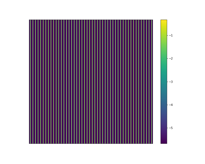
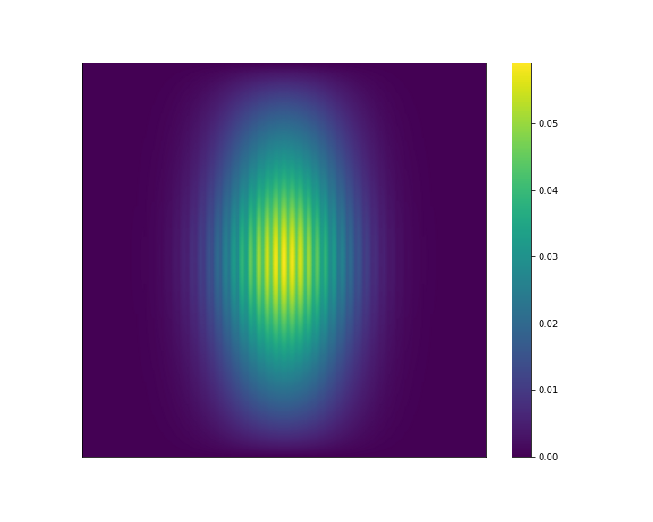
Figure 5: High-contrast part $\log(g_{2})$ (left) and reference solution (right) in example 1.

$H$	$l$	Type 1		Type 2		Type 3
		$e_{2}^{(1)}$	$e_{2}^{(2)}$	$e_{2}^{(1)}$	$e_{2}^{(2)}$	$e_{2}^{(1)}$	$e_{2}^{(2)}$
$\frac{1}{12}$	$\lceil-2\log(H)\rceil=5$	8.17e-02	7.60e-02	8.17e-02	7.60e-02	1.36e-06	5.45e-07
$\frac{1}{24}$	$\lceil-2\log(H)\rceil=7$	1.84e-02	1.49e-02	1.84e-02	1.49e-02	1.30e-07	7.64e-09
$\frac{1}{48}$	$\lceil-2\log(H)\rceil=8$	2.76e-03	2.31e-03	2.76e-03	2.31e-03	4.27e-08	3.56e-08

Table 1: Error comparison by different coarse mesh in example 1.

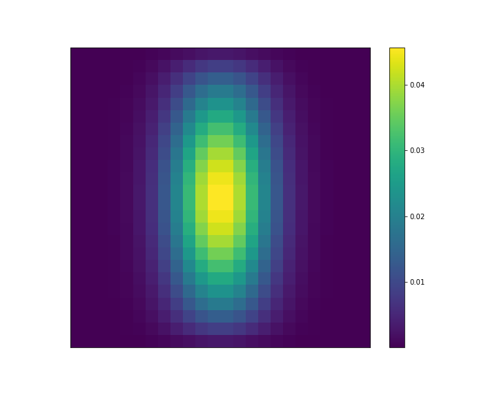
Figure 6: Average solution in example 1. Top-Left: Average reference solution in $\Omega_{1}$. Top-Right: Average reference solution in $\Omega_{2}$. Middle-Left: Average multicontinuum homogenization solution in $\Omega_{1}$. Middle-Right: Average multicontinuum homogenization solution in $\Omega_{2}$. Bottom-Left: Average hierarchical multicontinuum homogenization solution in $\Omega_{1}$. Bottom-Right: Average hierarchical multicontinuum homogenization solution in $\Omega_{2}$.

4.2 Example 2

In this example, we examine the high-contrast function $g_{2}$ with a crossed geometry, characterized by $\epsilon=1/48$. We depict the logarithm of the function $g_{2}$ and the reference solution in Figure 7. The errors obtained by refining the coarse mesh size are detailed in Table 2. We observe that our hierarchical algorithm has the same performance as the original multicontinuum homogenization method. The error decreases as the coarse mesh size decreases. Furthermore, the difference between these two approaches is negligible compared to the error stemming from the homogenization process. For example, the error due to homogenization can be as large as $10^{-3}$, while the difference between the two methods can be as small as $10^{-8}$ when $H=1/48$. To provide additional validation, we select representative average solutions, depicted in Figure 8, which further demonstrate the efficiency of our method.

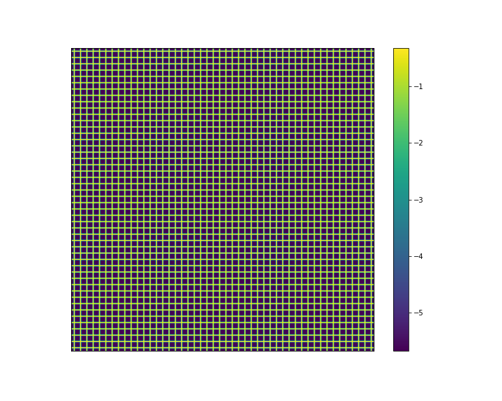
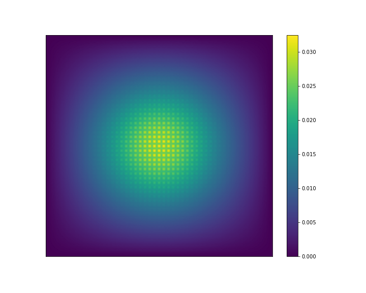
Figure 7: High-contrast part $\log(g_{2})$ (left) and reference solution (right) in example 2.

$H$	$l$	Type 1		Type 2		Type 3
		$e_{2}^{(1)}$	$e_{2}^{(2)}$	$e_{2}^{(1)}$	$e_{2}^{(2)}$	$e_{2}^{(1)}$	$e_{2}^{(2)}$
$\frac{1}{12}$	$\lceil-2\log(H)\rceil=5$	4.54e-02	4.53e-02	4.54e-02	4.53e-02	2.75e-06	2.52e-06
$\frac{1}{24}$	$\lceil-2\log(H)\rceil=7$	7.07e-03	6.22e-03	7.07e-03	6.22e-03	2.37e-07	1.43e-07
$\frac{1}{48}$	$\lceil-2\log(H)\rceil=8$	1.76e-03	1.40e-03	1.76e-03	1.40e-03	6.78e-08	6.05e-08

Table 2: Error comparison by different coarse mesh in example 2.

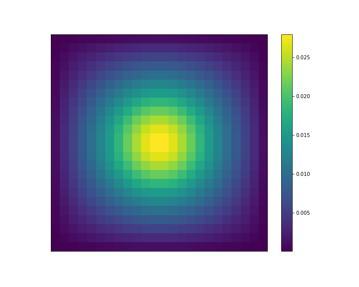
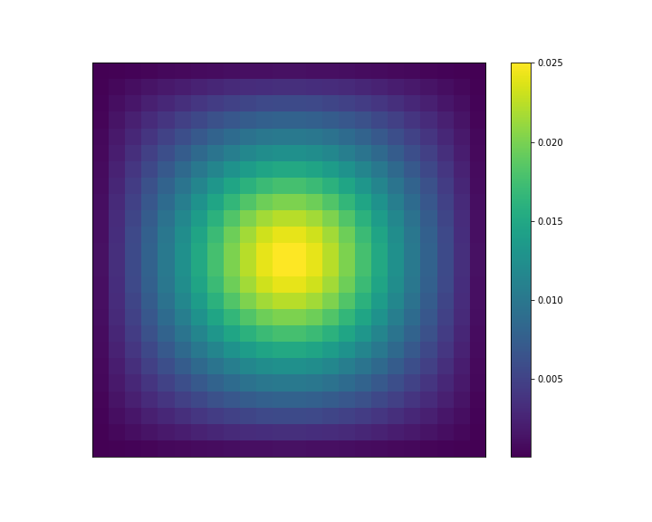
Figure 8: Average solution in example 2. Top-Left: Average reference solution in $\Omega_{1}$. Top-Right: Average reference solution in $\Omega_{2}$. Middle-Left: Average multicontinuum homogenization solution in $\Omega_{1}$. Middle-Right: Average multicontinuum homogenization solution in $\Omega_{2}$. Bottom-Left: Average hierarchical multicontinuum homogenization solution in $\Omega_{1}$. Bottom-Right: Average hierarchical multicontinuum homogenization solution in $\Omega_{2}$.

4.3 Example 3

In the third example, we consider a non-periodic high-contrast function $g_{2}$, with a contrast parameter of $\epsilon=1/30$. For clarity, we plot the logarithm of $g_{2}$ and the fine-grid solution in Figure 9. Accurately representing the different continua requires a very fine grid, and the non-periodic case further increases this demand. Due to the limitations of our computational resources, we test only two different coarse mesh sizes for the non-periodic structure. The results are detailed in Table 3. We observe that the homogenization error decreases as the coarse mesh size decreases. However, the hierarchical part failed to maintain the same property, but it can provide an acceptable accuracy, achieving a $10\%$ error for a given mesh size. In Figure 10, we plot the three different average solutions with $H=1/24$. From the figure, we observe that this is consistent with our error table.

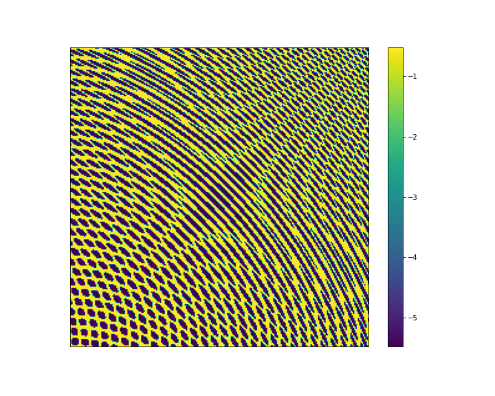
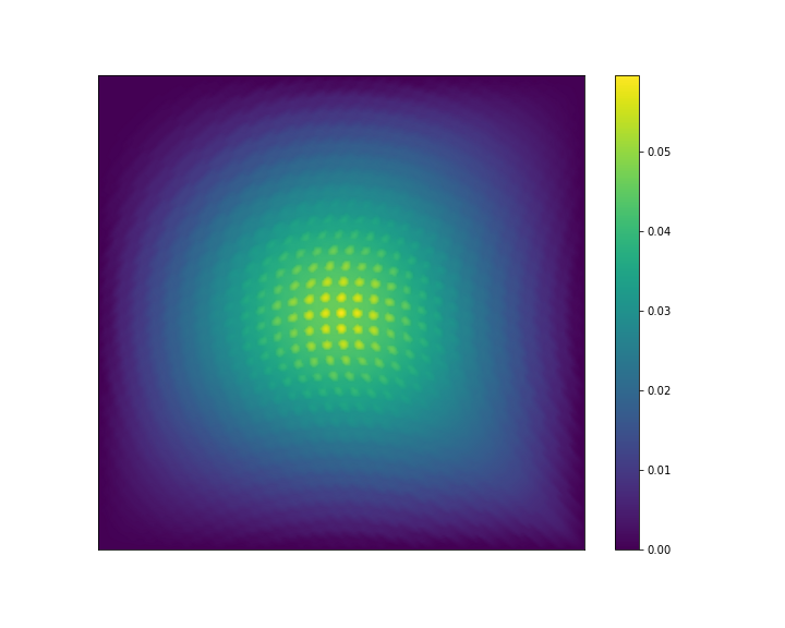
Figure 9: High-contrast part $\log(g_{2})$ (left) and reference solution (right) in example 3.

$H$	$l$	Type 1		Type 2		Type 3
		$e_{2}^{(1)}$	$e_{2}^{(2)}$	$e_{2}^{(1)}$	$e_{2}^{(2)}$	$e_{2}^{(1)}$	$e_{2}^{(2)}$
$\frac{1}{12}$	$\lceil-2\log(H)\rceil=5$	4.74e-02	4.70e-02	1.45e-01	1.03e-01	1.03e-01	6.11e-02
$\frac{1}{24}$	$\lceil-2\log(H)\rceil=7$	1.33e-02	1.07e-02	1.20e-01	8.06e-02	1.22e-01	8.37e-02

Table 3: Error comparison by different coarse mesh in example 3.

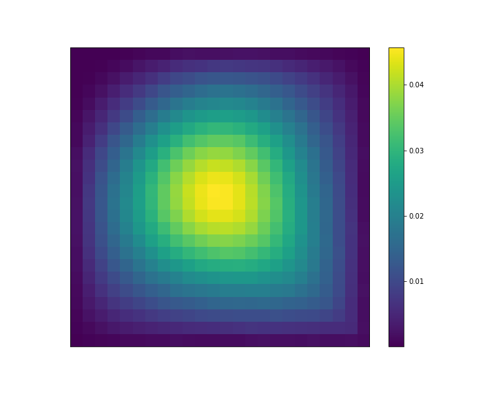
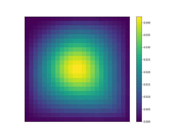
Figure 10: Average solution in example 3. Top-Left: Average reference solution in $\Omega_{1}$. Top-Right: Average reference solution in $\Omega_{2}$. Middle-Left: Average multicontinuum homogenization solution in $\Omega_{1}$. Middle-Right: Average multicontinuum homogenization solution in $\Omega_{2}$. Bottom-Left: Average hierarchical multicontinuum homogenization solution in $\Omega_{1}$. Bottom-Right: Average hierarchical multicontinuum homogenization solution in $\Omega_{2}$.

4.4 Example 4

In the last example, we consider another non-periodic configuration of $g_{2}$. The contrast parameter $\epsilon$ is $1/12$. The distribution of the two continua and the reference solution is depicted in Figure 11. For the same reason as in Example 3, we refine the coarse mesh only once. In Table 4, we provide details of the numerical errors. We observe that the error in the homogenization part decreases as we refine the coarse mesh. The error in the hierarchical part does not change but is kept within an acceptable tolerance, around $10\%$. In Figure 12, we show the average solutions of the fine-grid, multicontinuum homogenization, and hierarchical multicontinuum homogenization approaches. These figures are also consistent with our observations from the error table.

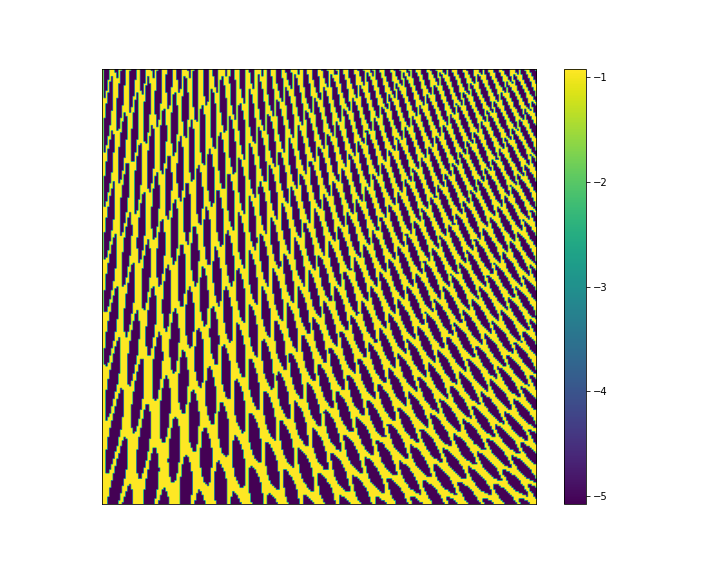
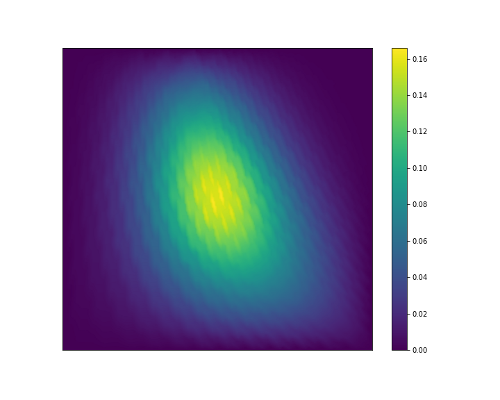
Figure 11: High-contrast part $\log(g_{2})$ (left) and reference solution (right) in example 4.

$H$	$l$	Type 1		Type 2		Type 3
		$e_{2}^{(1)}$	$e_{2}^{(2)}$	$e_{2}^{(1)}$	$e_{2}^{(2)}$	$e_{2}^{(1)}$	$e_{2}^{(2)}$
$\frac{1}{12}$	$\lceil-2\log(H)\rceil=5$	6.26e-02	6.41e-02	1.46e-01	1.33e-01	9.06e-02	7.54e-02
$\frac{1}{24}$	$\lceil-2\log(H)\rceil=7$	1.95e-02	2.26e-02	1.15e-01	1.02e-01	1.07e-01	9.44e-02

Table 4: Error comparison by different coarse mesh in example 4.

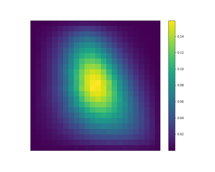
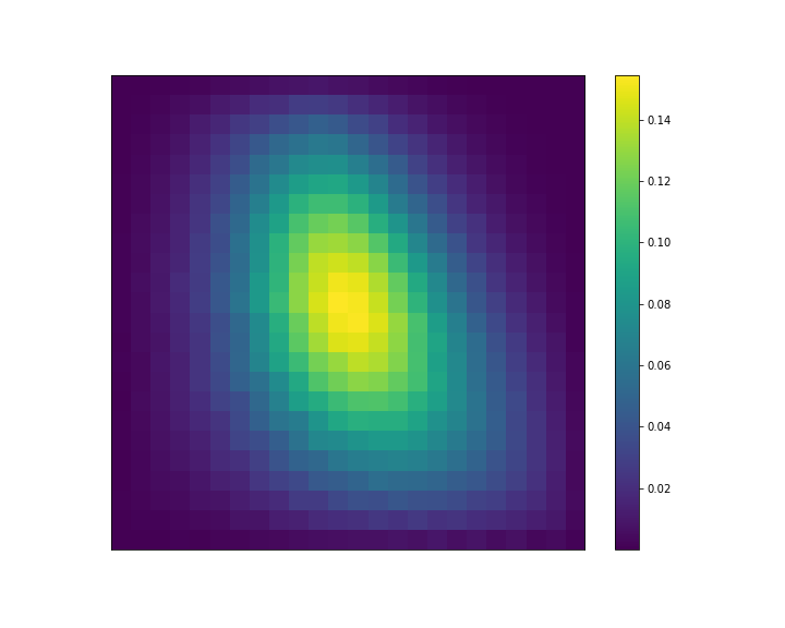
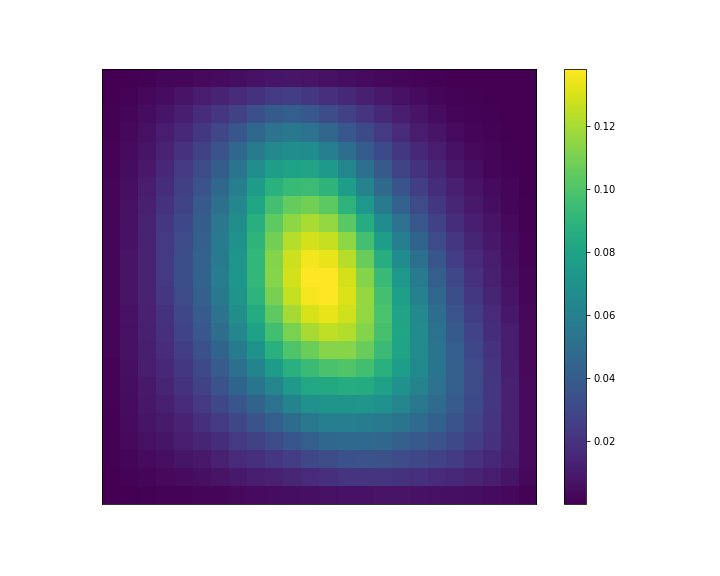
Figure 12: Average solution in example 4. Top-Left: Average reference solution in $\Omega_{1}$. Top-Right: Average reference solution in $\Omega_{2}$. Middle-Left: Average multicontinuum homogenization solution in $\Omega_{1}$. Middle-Right: Average multicontinuum homogenization solution in $\Omega_{2}$. Bottom-Left: Average hierarchical multicontinuum homogenization solution in $\Omega_{1}$. Bottom-Right: Average hierarchical multicontinuum homogenization solution in $\Omega_{2}$.

5 Conclusions

In this paper, we propose a hierarchical algorithm for the multicontinuum homogenization method to reduce computational cost by resolving the local solutions with a very fine mesh size at each macropoint. We outline the framework of the hierarchical multicontinuum homogenization method. Compared to the original multicontinuum homogenization method, we assume that the local solutions can be expressed as a combination of solutions at already-constructed macropoints and a correction function. Our approach consists of three main steps: First, we construct a hierarchical macropoint structure with dense properties. Second, we define a nested finite element (FE) space for the hierarchical macropoints. Lastly, the correction terms are computed within the corresponding FE spaces. We further analyze the computational complexity of the original multicontinuum homogenization method and our hierarchical approach. Numerical tests show that for permeability fields without significant orders of magnitude variations, our method is fully sufficient. Even when the permeability field exhibits large variations, our approach still achieves acceptable accuracy.

Acknowledgement

Wei Xie acknowledges support from the China Scholarship Council (CSC, Project ID: 202308430231) for funding during the visit to Nanyang Technological University (NTU). Sincere thanks to NTU for providing an outstanding working and learning environment that greatly advanced the research and professional development. Viet Ha Hoang is supported by the Tier 2 grant T2EP20123-0047 awarded by the Singapore Ministry of Education. Yin Yang is supported by the National Natural Science Foundation of China Project (No. 12071402, No. 12261131501), the Project of Scientific Research Fund of the Hunan Provincial Science and Technology Department (No. 2024JJ1008), and Program for Science and Technology Innovative Research Team in Higher Educational Institutions of Hunan Province of China. Yunqing Huang is supported by National Natural Science Foundation of China Key Program (12431014).

References

- [1] A. Abdulle, E. Weinan, B. Engquist, and E. Vanden-Eijnden. The heterogeneous multiscale method. Acta Numerica, 21:1–87, 2012.
- [2] A. Alikhanov, H. Bai, J. Huang, A. Tyrylgin, and Y. Yang. Multiscale model reduction for the time fractional thermoporoelasticity problem in fractured and heterogeneous media. Journal of Computational and Applied Mathematics, 455:116157, 2025.
- [3] H. Bai, D. Ammosov, Y. Yang, W. Xie, and M. A. Kobaisi. Multicontinuum modeling of time-fractional diffusion-wave equation in heterogeneous media. arXiv preprint arXiv:2502.09428, 2025.
- [4] D. L. Brown, Y. Efendiev, and V. H. Hoang. An efficient hierarchical multiscale finite element method for stokes equations in slowly varying media. Multiscale Modeling & Simulation, 11(1):30–58, 2013.
- [5] D. L. Brown and V. H. Hoang. A hierarchical finite element monte carlo method for stochastic two-scale elliptic equations. Journal of Computational and Applied Mathematics, 323:16–35, 2017.
- [6] V. M. Calo, Y. Efendiev, J. Galvis, and G. Li. Randomized oversampling for generalized multiscale finite element methods. Multiscale Modeling & Simulation, 14(1):482–501, 2016.
- [7] E. Chung, Y. Efendiev, J. Galvis, and W. T. Leung. Multicontinuum homogenization. general theory and applications. Journal of Computational Physics, 510:112980, 2024.
- [8] E. T. Chung, Y. Efendiev, and W. T. Leung. Constraint energy minimizing generalized multiscale finite element method. Computer Methods in Applied Mechanics and Engineering, 339:298–319, 2018.
- [9] E. T. Chung, Y. Efendiev, W. T. Leung, and M. Vasilyeva. Nonlocal multicontinua with representative volume elements. bridging separable and non-separable scales. Computer Methods in Applied Mechanics and Engineering, 377:113687, 2021.
- [10] E. T. Chung, Y. Efendiev, W. T. Leung, M. Vasilyeva, and Y. Wang. Non-local multi-continua upscaling for flows in heterogeneous fractured media. Journal of Computational Physics, 372:22–34, 2018.
- [11] E. T. Chung, Y. Efendiev, and G. Li. An adaptive gmsfem for high-contrast flow problems. Journal of Computational Physics, 273:54–76, 2014.
- [12] D. Cioranescu and P. Donato. An introduction to homogenization. Oxford university press, 1999.
- [13] Y. Efendiev, J. Galvis, and T. Y. Hou. Generalized multiscale finite element methods (gmsfem). Journal of Computational Physics, 251:116–135, 2013.
- [14] Y. Efendiev and W. T. Leung. Multicontinuum homogenization and its relation to nonlocal multicontinuum theories. Journal of Computational Physics, 474:111761, 2023.
- [15] Y. Efendiev, W. T. Leung, B. Shan, and M. Wang. Multicontinuum splitting scheme for multiscale flow problems. arXiv preprint arXiv:2410.05253, 2024.
- [16] S. Fu, E. Chung, and L. Zhao. An efficient multiscale preconditioner for large-scale highly heterogeneous flow. SIAM Journal on Scientific Computing, 46(2):S352–S377, 2024.
- [17] P. Henning and A. Målqvist. Localized orthogonal decomposition techniques for boundary value problems. SIAM Journal on Scientific Computing, 36(4):A1609–A1634, 2014.
- [18] P. Henning and M. Ohlberger. The heterogeneous multiscale finite element method for elliptic homogenization problems in perforated domains. Numerische Mathematik, 113:601–629, 2009.
- [19] U. Hornung. Homogenization and porous media, volume 6. Springer Science & Business Media, 2012.
- [20] T. Hou, X. Wu, and Z. Cai. Convergence of a multiscale finite element method for elliptic problems with rapidly oscillating coefficients. Mathematics of Computation, 68(227):913–943, 1999.
- [21] T. Y. Hou and X. Wu. A multiscale finite element method for elliptic problems in composite materials and porous media. Journal of Computational Physics, 134(1):169–189, 1997.
- [22] S. Jiang, M. Sun, and Y. Yang. Reduced multiscale computation on adapted grid for the convection-diffusion robin problem. Journal of Applied Analysis and Computation, 7(4):1488–1502, 2017.
- [23] A. Målqvist and D. Peterseim. Localization of elliptic multiscale problems. Mathematics of Computation, 83(290):2583–2603, 2014.
- [24] J. S. R. Park and V. H. Hoang. Hierarchical multiscale finite element method for multi-continuum media. Journal of Computational and Applied Mathematics, 369:112588, 2020.
- [25] Z. Wang, C. Ye, and E. T. Chung. A multiscale method for inhomogeneous elastic problems with high contrast coefficients. Journal of Computational and Applied Mathematics, 436:115397, 2024.
- [26] W. Xie, Y. Efendiev, Y. Huang, W. T. Leung, and Y. Yang. Multicontinuum homogenization in perforated domains. Journal of Computational Physics, page 113845, 2025.
- [27] W. Xie, J. Galvis, Y. Yang, and Y. Huang. On time integrators for generalized multiscale finite element methods applied to advection–diffusion in high-contrast multiscale media. Journal of Computational and Applied Mathematics, 460:116363, 2025.
- [28] W. Xie, Y. Yang, E. Chung, and Y. Huang. Cem-gmsfem for poisson equations in heterogeneous perforated domains. Multiscale Modeling & Simulation, 22(4):1683–1708, 2024.
- [29] C. Ye and E. T. Chung. Constraint energy minimizing generalized multiscale finite element method for inhomogeneous boundary value problems with high contrast coefficients. Multiscale Modeling & Simulation, 21(1):194–217, 2023.
- [30] C. Ye, H. Dong, and J. Cui. Convergence rate of multiscale finite element method for various boundary problems. Journal of Computational and Applied Mathematics, 374:112754, 2020.
- [31] C. Ye, S. Fu, E. T. Chung, and J. Huang. A robust two-level overlapping preconditioner for darcy flow in high-contrast media. SIAM Journal on Scientific Computing, 46(5):A3151–A3176, 2024.